Simulating Fully 3D Hydraulic Fracturing

B.J. Carter†, J. Desroches‡, A.R. Ingraffea†, and P.A. Wawrzynek†

†Cornell University, Ithaca, NY

‡Schlumberger Well Services, Houston, TX 1.0 Introduction

Hydraulic fracturing, the process of initiation and propagation of a crack by pumping fluid at

relatively high flow rates and pressures, is one of several techniques for creating cracks in rock.

Fractures in the earth's crust are desired for a variety of reasons, including enhanced oil and gas

recovery, re-injection of drilling or other environmentally sensitive wastes, measurement of in

situ stresses, geothermal energy recovery, and enhanced well water production. These fractures

can range in size from a few meters to hundreds of meters, and their cost is often a significant

portion of the total development cost. In locations where the in situ stress field, including the

directions, is known and the wellbore is aligned with one of the far-field principal stresses, the

hydraulic fracture geometry can be predicted and controlled with reasonable accuracy. For those

wellbores that are not aligned with such a direction (deviated wells), the hydraulic fracture

geometry is usually more complex and more difficult to model, especially close to the wellbore

where the local stress field is significantly different from the far-field stresses. Field data from

hydraulic fracturing operations exist primarily in the form of pressure response curves. It is

difficult to define the actual hydraulic fracture geometry from this data alone, however.

Therefore, numerical simulations are used to evaluate and predict the location, direction and

extent of these hydraulic fractures.

Simulations range from two to fully three dimensional depending on the degree of complexity of

the wellbore and fracture geometries, the capability of the available simulator, and the required

accuracy of the predictions. Numerous 2D, pseudo-3D, and planar 3D hydraulic fracturing

simulators exist, and these simulators work very well in many cases where the geometry of the

fracture is easily defined and constrained to a single plane. However, there are instances where a

fully 3D simulator is necessary for more accurate modeling. For example, fractures from

deviated wellbores are generally non-planar with arbitrary crack front shapes. Most

hydrofracturing simulators simply ignore the near-wellbore effects of deviated wells and assume

a planar starting crack that has extended beyond this region. The problem with this approach is

that most of the difficulties and failures in hydraulic fracturing of deviated wellbores can be

attributed to restricted flow in the near-wellbore region. Restricted flow usually is due to fracture

reorientation and interaction with other fractures. Hydraulic fracturing of deviated wells, where

the fractures reorient as they propagate, clearly requires fully 3D simulation capabilities and

accurate modeling of the near-wellbore geometry.

Efficient numerical simulation of fully 3D hydraulic fracturing requires at least two key

components. The first is a capability for representing and visualizing the complex wellbore and

fracture geometries. The second is a method for solving the highly non-linear coupling between

the equations for the fluid flow in the fracture and the deformation and propagation of the

fracture. The first component can be partitioned into several sub-components, including

geometrical and topological solid modeling tools, routines to model geometry and topology

changes for fracture propagation, automated meshing and remeshing capabilities, visualization of

response information, and analysis control information (i.e. input for a stress analysis program).

The second component consists of a stress analysis procedure, fluid flow simulation capabilities,

and a method for coupling the structural response with the fluid flow, including rules for

determining hydraulic fracture propagation direction and extent. The authors have developed a

simulator that includes all of these components for modeling multiple, non-planar, fully 3D,

hydraulic fracture propagation. This simulator treats hydraulic fracturing as a quasi-static

process, and the solution consists of a series of “snapshots in time” of the fracture geometry,

fluid pressures, and crack opening displacements.

A brief history of hydraulic fracturing and the development of hydrofracturing simulators are

discussed in the next section. Then the key components of the new simulator are described in

some detail, including the software framework for model representation, the coupled elasticity

and lubrication theory, the finite element implementation of this theory, and the iterative solution

procedure. The simulator has been verified for a radial (penny-shape) and a slot-like (part-

through) fracture by comparing results to those from a robust and accurate 2D simulator,

Loramec (Desroches and Thiercelin, 1993). Further simulations that compare well with

experimental results show the ability of the system to model more realistic hydraulic fracture

geometries. This chapter concentrates on the development of the simulator rather than actual

simulations, however. Detailed simulations of hydraulic fracturing from cased, perforated,

deviated wellbores is possible now, but is computationally intensive and is left as the subject of

future publications.

2.0 Background

The process of hydraulic fracturing is not new. Nature has produced many such fractures in the

earth's crust (see for example Bahat, 1991). The first recorded application of hydraulic fracturing

for enhancing oil recovery that the authors are aware of was in 1947 in Kansas (see Howard and

Fast, 1970). The "Hydrafrac" concept was formalized first by Clark (1949), although others had

recognized previously that "pressure parting" could occur during acid treatment and water

injection, a phenomenon considered to be closely related to the "Hydrafrac" concept (Howard

and Fast, 1970). The Hugotan field in western Kansas was the site of the first hydraulic

fracturing operation, and by the mid-1960's, hydraulic fracturing had become the dominant

method of stimulation in this and many other fields (Howard and Fast, 1970).

During this early period of hydraulic fracturing, two simple models were proposed to try to

predict the shape and size of a hydraulic fracture based on the rock and fluid properties, the

pumping parameters, and the in situ stresses (Khristianovic and Zheltov, 1955; Geertsma and de

Klerk, 1969; Perkins and Kern, 1961; Nordgren, 1972). The models are known as the KGD and

PKN models, and their description can be found in the above references and in many other

summaries or texts (eg. Geertsma, 1989; Mendelsohn, 1984a,b). Perkins and Kern (1961) and

Geertsma and de Klerk (1969) also derived a model for radial hydraulic fracturing. The radial,

KGD, and PKN models are essentially two dimensional plane strain formulations with fluid flow

only along the length (or radius) of the fracture. The fracture width and shape are related to the

fluid pressure distribution in the fracture; the KGD model has a constant height and constant

width through the height, while the PKN model has a constant height and an elliptical vertical

cross-section.

The 2D models are not able to simulate both vertical and lateral propagation. Therefore, pseudo-

3D models were formulated by removing the assumption of constant and uniform height (Settari

and Cleary, 1986; Morales, 1989). The height in the pseudo-3D models is a function of position

along the fracture as well as time. The major assumption is that the fracture length is much

greater than the height, and an important difference between the pseudo-3D and the 2D models is

the addition of a vertical fluid flow component. The pseudo-3D models have been used to model

fractures through multiple rock layers with differing stresses and properties. These models are

simple, fast, and relatively effective. Warpinski et al. (1994) recently provided brief descriptions

and a comparison of predictions for a number of simulators, including 2D and pseudo-3D

models.

Pseudo-3D models cannot handle fractures of arbitrary shape and orientation, however; fully 3D

models are required for this purpose. The literature contains numerous references to fully 3D

simulators; the majority of these are limited to planar fracture surfaces, however. These are

called planar-3D simulators in this chapter to differentiate them from true fully 3D simulators

which can model out-of-plane fracture growth. Planar-3D simulators have been developed by

Clifton and Abou-Sayed (1979), Barree (1983), Touboul et al. (1986), Morita et al. (1988),

Advani et al. (1990), and Gu and Leung (1993). Out of plane 3D hydraulic fracture growth has

been modeled by Lam et al. (1986), Vandamme and Jeffrey (1986), and Sousa et al. (1993). To

the authors’ knowledge, only Carter et al. (1994), using the predecessor of the simulator

described herein, have modeled 3D fracture in the near-wellbore region of a cased, perforated,

and deviated wellbore.

The increasing use of deviated wellbores implies that fully 3D hydraulic fracture simulators are

vital to the petroleum industry. Hydrofracturing is often less effective for deviated wellbores as

compared to traditional vertical wells. Some of the problems have been attributed to a poor

understanding of the mechanics of fracture initiation and propagation from a deviated wellbore.

The complex state of stress which is generated around an inclined wellbore (Yew and Li, 1988;

Ong and Roegiers, 1995) means that the fracture propagates with a complex geometry

(Behrmann and Elbel, 1990; Hallam and Last, 1991; Weijers and de Pater, 1992; Abass et al.,

1996). The complex stress state and fracture geometry can limit the fracture width at the

wellbore and hinder the injection of proppant into the fracture leading to premature screenout

(Hallam and Last, 1991; Soliman et al., 1996). Nevertheless, the advantages of drilling inclined

wellbores are significant. For example, the ability to drill several wells from a single location

minimizes production infrastructure and impact on the environment. Therefore, the ability to

model hydraulic fracturing from deviated wells is of ever increasing importance.

In addition to inadequate modeling of the fracture geometry, many of the current hydraulic

fracturing simulators do not predict the correct wellbore fluid pressure or fracture geometry even

for planar fractures. The proposed reasons for this are numerous (Medlin and Fitch, 1983;

Warpinski, 1985; Shlyapobersky et al., 1988; Jeffrey, 1989; Palmer and Veatch, 1990; Johnson

and Cleary, 1991; Gardner, 1992; Papanastasiou and Thiercelin, 1993; de Pater et al., 1993 and

van den Hoek et al., 1993). The simulator developed here addresses this problem by properly

modeling the near crack tip behavior (SCR, 1993). Furthermore, the simulator is ideal for

modeling non-planar hydraulic fracturing, and is able to model multiple branching, intersecting,

and merging fractures as will be shown in the following section.

3.0 Model Representation

The first key component of an efficient, fully 3D, hydraulic fracture simulator is the geometric

representation of the model. Representation implies computer storage and visualization of the

model topology and geometry. This portion of the hydraulic fracture simulator is actually a

general purpose, fully 3D, fracture analysis code, called FRANC3D, under development at

Cornell University since 1987 (Martha, 1989; Wawrzynek, 1991; Potyondy, 1993). FRANC3D

is capable of modeling multiple, arbitrary, non-planar, 3D cracks in complex structures, and has

pre- and post-processing capabilities for both finite and boundary elements. It relies on a

boundary surface representation of the model and a radial edge data structure for storing and

accessing topological and geometrical information. It has the ability to do fully automatic or

fully user-controlled crack growth simulations, including post-processing of the response

information, modifying the geometry, remeshing, and updating the boundary conditions for each

stage of crack growth. The complex geometry associated with perforated, cased, and deviated

wellbores with multiple non-planar evolving 3D cracks requires a sophisticated, but easy to use

simulation capability. FRANC3D has these capabilities, and some of its individual components

are described briefly in the following sections.

3.1 Representational Model of Fracture Propagation

Crack growth simulation in FRANC3D is an incremental process, where a sequence of

operations is repeated for a progression of models (Figure 1). Each step in the process relies on

previously computed results and represents one crack configuration. There are four primary

collections of data, or databases, required for each step. The first is the representational database,

denoted Ri (where the subscript identifies the step). The representational database contains a

description of the solid model geometry, including the cracks, the boundary conditions, and the

material properties. The representational database is transformed by a discretization (or meshing,

M ) process to a stress analysis database Ai . The analysis database contains a complete, but

approximate description of the body, suitable for input to a solution procedure (S ), usually a

finite or boundary element stress analysis program.

The solution procedure is used to transform the analysis database to an equilibrium database Ei

which consists of field variables, such as displacements and stresses, that define the equilibrium

solution for the analysis model Ai . The equilibrium model should contain field variables and

material state information for all locations in the body, and in the context of a crack growth

simulation, should also contain values for stress-intensity factors, or other fracture parameters Fi

for all crack fronts. The equilibrium database is used in conjunction with the current

representational database to update (U(C)) the representational model Ri+1 including the

increment of crack growth as governed by the fracture parameters Fi and the crack growth

function C . This process is performed repeatedly (Figure 1) until a suitable termination

condition is reached.

FRANC3D encompasses all components of this conceptual model except for the stress analysis

procedure (Figure 2). The individual components consist of unique databases and functions that

operate on the databases, some of which are described in more detail in the following sections.

3.2 Solid Modeling For Crack Growth Simulations

Simulation of crack growth is more complicated than many other applications of computational

mechanics because the geometry and topology of the structure evolve during the simulation. For

this reason, a geometric description of the body that is independent of any mesh needs to be

maintained and updated as part of the simulation process. The geometry database should contain

an explicit description of the solid model including the crack. The three most widely used solid

modeling techniques, boundary representation (B-rep), constructive solid geometry (CSG), and

parametric analytical patches (PAP) (Hoffmann, 1989; Mäntylä, 1988; Mortenson; 1985), are

capable of representing uncracked geometries. A B-rep modeler stores surfaces and surface

geometries explicitly. If explicit topological adjacency information (as defined in the next

section) is available as well, two topologically distinct surfaces can share a common geometric

description. Cracks, for instance, consist of two surfaces that have the same geometric

description; for this reason, among others, a boundary representation was found to be the most

suitable of the three modeling techniques for modeling cracks.

3.3 Computational Topology as a Framework for Crack Growth Simulation

Explicit topological information is an essential feature of the representational database for crack

growth simulations. The topology of an object is the information about relationships, proximity,

and order among features of the geometry—incomplete geometric information. These are the

properties of the actual geometry that are invariant with respect to geometric transformations; the

geometry can change, but the topology remains the same (Figure 3). A topology framework

serves as an organizational tool for the data that represents an object and the algorithms that

operate on the data.

There are several reasons for using a topological representation for crack growth simulation: 1)

topological information, unlike geometrical information, can be stored exactly with no

approximations or ambiguity; 2) there are formal and rigorous procedures for storing and

manipulating topology data (Mäntylä, 1988; Hoffmann, 1989; Weiler, 1986); 3) any topological

configuration can represent an infinite number of geometrical configurations; and 4) topology

generally changes much less frequently than the geometry during crack propagation.

Investigations into the use of data structures for storing information needed for crack propagation

simulations (Wawrzynek and Ingraffea 1987a,b) showed that topological databases were a

convenient and powerful organizing agent, and efficient topological adjacency queries make this

data structure ideally suited for interactive modeling.

Explicit topological information is used as a framework for the representational database Ri and

aids in implementation of the meshing function M and the updating function U(C) . In

particular, by using a topological database in conjunction with a B-rep modeler, topological

entities can serve as the principal elements of the database with geometrical descriptions and all

other attributes (such as boundary conditions and material properties) accessed through the

topological entities.

Several topological data structures have been proposed for manifold objects: the winged-edge

(Baumgart, 1975), the modified winged-edge, the face-edge, the vertex-edge (Weiler, 1985), and

the half-edge (Mäntylä, 1988) data structures. However, these data structures cannot be used for

modeling fully 3D hydraulic fracturing because features like bi-material interfaces create non-

manifold topologies. Weiler (1986) presented another edge-based data structure for storing non-

manifold objects, called the radial-edge, and outlined the corresponding generalized non-

manifold Euler operators. The basic topological entities used for modeling are vertices, edges,

faces, and regions. An internal crack, for example, consists of vertices, edges, and faces with a

null volume region between the crack surfaces. The edge entity is the object through which

topological relationships are maintained and queried (Figure 4). As the name implies, the edge

uses are ordered radially about the edge; each face has two face uses and each face use has a

corresponding edge use on the given edge. The radial ordering allows for efficient storage,

querying and manipulation of the model topology. As shown in Figure 5, this data structure, in

addition to bi-material interfaces, is clearly able to represent model topologies consisting of

branching or intersecting cracks; both are important features when modeling hydraulic fracturing

in a layered rock mass from a cased and deviated wellbore.

A crack is defined within this representational database by both geometry and topology. It

consists of multiple surfaces in order to represent the evolving geometry as well as the possibility

of intersecting, branching, and merging cracks. Crack surfaces are arranged in pairs (main and

mate surface, see Figure 5), and each surface is composed of faces, edges and vertices. The

edges and vertices are further classified based on their location on the crack surface. For

instance, crack front edges represent the leading edge of the crack within the solid. Note that

crack growth involves modifying the model topology and geometry to represent newly created

fracture surfaces.

3.4 Meshing, Crack Growth and Model Update Functions

The combination of the boundary representation solid model and the radial edge topological

database comprises the representational model Ri . Complex 3D models of deviated, perforated,

and cased wellbores including multiple non-planar fractures can be built fairly quickly and easily

using this representational model. The other components of the abstract model, such as the

discretization (meshing), crack growth and model updating, post-processing, and visualization

also take advantage of the topological database. The meshing capabilities (Potyondy et al., 1995)

and the crack growth and model update functions (Martha et al., 1993; Carter et al., 1997) in

FRANC3D have been described elsewhere. For completeness however, a brief description of

both functions is needed here as they relate to modeling hydraulic fracturing.

FRANC3D maintains a consistent geometric representation of the model at each step of

propagation. During fracture propagation, the previous crack surface geometry remains the

same; new fracture surface is simply added to the model to represent the crack growth (Figure 6).

There are some exceptions when it is necessary to rebuild the entire fracture geometry, but this is

beyond the scope of the present discussion. Therefore, the mesh that is attached to the existing

geometric crack surfaces is unaffected by fracture growth because the existing geometry does not

change. In truth, the mesh is removed from the geometric crack surface during propagation, but

an identical mesh can be regenerated on that surface. A new mesh is attached to the new crack

surface. Thus, the process of modeling crack propagation involves neither a "fixed" nor a

"moving" mesh as described in other hydraulic fracturing literature. The mesh on the existing

crack surface can remain fixed or it can be modified, but a new mesh must be added to the new

crack surface. Mapping of information from the previous step of propagation to the current step

is discussed later.

4.0 The Physics and Mechanics of Hydraulic Fracturing

The second important component of a robust and accurate, fully 3D, hydraulic fracture simulator

is the ability to properly model the fluid flow coupled with the fracture deformation and

propagation. The following discussion is restricted to the framework of linear elasticity and

lubrication theory.

4.1 Elastic Stress Analysis

BES is a linear elastic, 3D, boundary element program (Lutz, 1991). It is based on a direct

formulation and uses special hypersingular integration techniques and non-conforming elements

on and around the crack surfaces. It is capable of handling multiple loading cases, specifically

generating basic solutions (displacements and tractions) for unit tractions at points on the crack

surface. Unit tractions are applied to each node on the discretized crack surface. The traction is

distributed according to the shape functions of the incident elements, starting at unity at the given

node and vanishing to zero at all adjacent nodes. The displacements at all nodes in the structure

are evaluated for each unit traction loading case, providing a matrix of solutions whose generic

element Kij is the displacement at node i due to a unit traction at node j .

The set of basic solutions is combined to build a single influence matrix which then is used along

with the equilibrium fluid pressures to determine the overall structural response due to both the

far field boundary conditions and the fluid pressure in the crack. The displacements in the

structure can be computed by multiplying each of the basic solutions, obtained for a unit traction

at a node, by the fluid pressure at that node. This means that the stress analysis, which is the

most time consuming process of the entire simulation, can be performed once for a specific

model or crack geometry. Various fluid properties and flow parameters then can be used in the

hydraulic fracture simulator based on this single stress analysis.

4.2 Fluid Flow

A peculiarity of hydraulic fracturing consists of the strong nonlinear coupling between fluid flow

and solid deformation, particularly in the vicinity of the fracture front. Proper coupling, as

derived by the Geomechanics Group at Schlumberger Cambridge Research (SCR, 1993, 1994),

yields an analytical model for pressure and width near the crack front which corresponds to a

stress singularity that is different from the usual linear elastic fracture mechanics solution

(LEFM). A new term has been coined, linear elastic hydraulic fracturing (LEHF), to reflect the

difference in the solutions. The use of the LEHF analytical model provides an elegant solution to

the numerical problem otherwise associated with modeling the front of a hydraulic fracture.

(Note that a 3D crack front becomes a crack tip in 2D.)

4.2.1 Review of 2D LEHF Solution

Following an approach similar to Spence and Sharp (1985), the Geomechanics Group at SCR

(SCR, 1993) has shown that a fluid lag often develops near the crack tip, and this fluid lag

negates the influence of the rock fracture toughness. However, by assuming that the fluid

reaches the crack tip, a particular singularity develops in both the fluid pressure and the stress

field ahead of the crack tip which is unique to hydraulic fracturing (SCR, 1994). This yields an

intermediate asymptotic solution for the width and pressure in the crack which is independent of

fracture toughness, provided that more energy is dissipated in the fluid than in creating new

fracture surface. It is intermediate in the sense that there exists a small region at the very tip of

the fracture where a fluid lag develops and LEFM holds, but has little effect on the rest of the

solution and is not taken into account.

To obtain the general solution for fluid flow in the vicinity of the tip of a hydraulic fracture

propagating in an impermeable solid, the following assumptions are made: crack propagation is

self-similar and steady-state, the rock mass is a linear elastic solid in plane strain, lubrication

theory is valid, and the fluid is incompressible with a power-law shear-thinning consistency. The

boundary conditions include the far-field minimum principal stress, the fracture width at the

crack tip, which must be zero, and the fluid velocity at the crack tip where the tip is a moving

boundary. Details of how the solution is obtained can be found in SCR (1994). The final

expressions for the pressure p and crack opening w in the vicinity of the crack tip, are as

follows:

p − σ3 = ph2 2 2 + ′ n ( )

π(2 − ′ n )

Lh

L

′ n /(2 + ′ n )

−Lh

ξ

′ n / (2+ ′ n )

(1)

w = ξ 2 /(2 + ′ n )Lh′ n /(2 + ′ n ) c1 ( ′ n ) − c2( ′ n )

ξL

2+ 3 ′ n 4+2 ′ n

(2)

where

Lh = V′ K ′ E

1/ ′ n

(3)

is a characteristic length particular to hydraulic fracturing and

ph = ′ E cos((1− α )π )

sin(απ )

1+ ′ n 2 ′ n +1

′ n 2 (2 + ′ n )

′ n

1 (2 + ′ n )

(4)

is a characteristic pressure with α ( ′ n ) = 2 (2 + ′ n ) . V is the crack tip speed which is equal to

the fluid velocity at the tip. L is the fracture half length and ξ is the position from the crack tip.

σ 3 is the far-field minimum stress. ′ E = E (1 − ν2 ) is the effective Young's modulus where E

is the Young's modulus and ν is Poisson's ratio. ′ K is the consistency index and ′ n is the

power-law exponent. c1 and c2 are constants (SCR, 1994) that are evaluated best numerically;

for a Newtonian fluid, they are c1 ≅ 7.21 and c2 ≅ 3.17. Note that the flow rate at the tip qb is a

function of the speed and the crack opening, qb = V ⋅w = f (V) .

From these equations, the fluid pressure at the crack tip is found to be singular; for a Newtonian

fluid, ′ n = 1 and the order of the singularity is 1/3. The stress at the crack tip has the same order

of singularity. The order of the singularity depends on the fluid properties only and, within the

assumptions made here, is always weaker than the 1/2 obtained from linear elastic fracture

mechanics.

A similar solution was developed for the permeable case and can be found in Lenoach (1995). It

involves a supplementary length scale because of the leak-off process and yields a solution which

exhibits yet another singularity, also weaker than that of linear elastic fracture mechanics.

4.2.2 Extension of the LEHF Solution to 3D

The behavior of a hydraulic fracture in the vicinity of its propagating front is easily described by

the LEHF solution, provided two additional assumptions are made: the crack front is considered

to be locally under plane strain conditions, and the local fluid flow parallel to the crack front is

negligible. We shall restrict ourselves to the case of a Newtonian fluid, but the process can easily

be extended to power-law fluids. The width w in the vicinity of the fracture front is then

described by the LEHF solution along any normal to the crack front:

w = (2) 37 6( ) µV′ E

1 3

ρ2 3 = β V1 3 (5)

where β = (2) 37 6( ) µ′ E

1 3

ρ2 3 and ρ is the curvilinear distance, measured on the fracture

surface, between any point and the fracture front. µ is the fluid viscosity.

The equation describing the mass conservation within the bulk of the fracture can then be

transformed in order to accommodate the introduction of the LEHF solution. The fracture is

considered as a surface in 3D space, F . Consider a subdomain Ω of the fracture, characterized

by a boundary Γ , a pressure field p , an aperture field w and fluid flux field q . t is the time.

If one considers any closed domain A included in Ω (Figure 7), fluid enters and leaves A

through its boundary ∂A . Fluid is stocked by an increase of the fracture width w with time t .

Considering also a source term at a point O included in A (injection or sink of value Q(t ) ),

one then can write for an incompressible fluid:

q ⋅ n d∂A∂ A +

∂w∂ t

dAA = Q(t)at O (6)

After transformation of the contour integral into a surface integral, one gets

(∂w∂ tA

+ divq − Q(t)δ(O))dA = 0 (7)

where δ is the Dirac operator. This equation must hold whatever the chosen domain A , which

yields the mass conservation equation for any point inside the considered domain Ω :

∂w∂ t

+ divq = Q( t)δ(O) (8)

One can write a variational equation for (8) by considering an auxiliary pressure field δp :

δp∂w∂ tΩ

dΩ + δp divq dΩΩ = Q(t )δP(O) (9)

Using s as the curvilinear abscissa along the boundary Γ and ns as the outward normal to Γ at

point s (Figure 7), one can apply the divergence theorem to the second integral of equation (9),

to get

δpΩ divq dΩ = − q ⋅grad(δp)

Ω dΩ + δp qΓ ⋅ns( )

Γ ds (10)

The lubrication approximation for a Newtonian fluid of viscosity µ gives

q = −w3

12µgradp (11)

Setting qΓ ⋅ ns = qb (Figure 7) and plugging the lubrication equation into equation (9), it becomes

δp∂w∂ tΩ

dΩ + (w3

12µΩ gradp) ⋅(gradδp) dΩ + δp

Γ qb dΓ = Q( t)δp(O) (12)

As illustrated in Figure 7, it is convenient to choose Ω so as to describe the bulk of the fracture,

whereas F -Ω corresponds to the domain of the fracture in the vicinity of the crack front that is

described by the LEHF solution. As Γ now is the boundary between Ω and the front region of

the fracture where the asymptotic solution holds, then

qb = V w (13)

where V is the velocity of the crack and w is now a known function of V and the distance ρ

from the crack front. Therefore, qb = β V 4 3 , which gives the final fluid flow equation to be

solved outside the vicinity of the crack front:

δp∂w∂ tΩ

dΩ + (w3

12µΩ (gradp ⋅ gradδp) dΩ + δp

Γ β V4/ 3 dΓ = Q( t)δp(O) (14)

The first two integrals correspond to the usual hydraulic fracture solution. The third integral is a

contour integral that incorporates the asymptotic solution for the fluid flow. The right hand side

accommodates the boundary condition of a source term at any point and can be extended for the

case of a line source.

5.0 Finite Element Implementation of Fluid Flow Coupled with the Structural Response

The finite element method is used to solve the fluid flow equation coupled with the structural

response. The special form of the fluid flow equation developed in section 4 allows one to

separate the fracture surface in two regions: the bulk of the fracture Ω where width and pressure

are to be determined and regular shell finite elements are used, and the near vicinity of the crack

front where special tip elements adjacent to the crack front are used. Thanks to the form of

equation (14), the special tip elements only represent the LEHF solution, and nodal width and

pressure are never computed, except at the boundary Γ between the regular elements and the tip

elements.

5.1 Finite Element Formulation of Fluid Flow Equation

Considering a set ofn shape functions N over the domain Ω, the pressure can be approximated

in the finite element sense by p = Nii =1i =n ˆ p i where ˆ p i is the pressure at node i (or in matrix form

p = N Tˆ p ). The small increment in pressure δp is approximated in a similar way

δp = Nii=1i=n δ ˆ p i . These two expressions, when introduced into (14), lead to

Niδˆ p ii=1

i =n

Ω

∂w∂t

dΩ + w3

12µΩ grad N j ˆ p j

j =1

j = n

⋅grad Niδˆ p i

i =1

i= n

dΩ

+ Niδˆ p ii =1

i = n

Γ β V4 / 3 dΓ = Q( t) Ni(O)Q(t)

i =1

i = n

(15)

Requiring stationarity of (15) leads to a set of n differential equations. Introducing the finite

element approximation for the width w together with the time discretization, the i -th equation

can be written as:

NiΩ N j

ˆ w j( tn +1) − ˆ w j (tn)tn +1 − tnj =1

j =n

dΩ

+1

12µNk ˆ w k

k=1

k =n

Ω

3

gradNi ⋅ grad N j ˆ p jj =1

j =n

dΩ

+ Ni β V4 3

Γ dΓ = Q(t)Ni (O)

(16)

where ˆ w j is the value of the width w at node j .

For simplicity, the i -th shape function is associated with the node at which it takes a value of 1.

It is worth noting that a shape function Ni is equal to zero when the point considered for the

integration is not part of an element containing the associated i -th node. Therefore, the integrals

in (16) can be reduced to integrals over a single element Ω i .

NiΩ i

N j

ˆ w j (tn+1 ) − ˆ w j( tn)tn+1 − tnj =1

j = n

dΩ

+1

12µNk ˆ w k

k =1

k= n

Ω i

3

gradNi ⋅ grad N j ˆ p jj =1

j = n

dΩ

+ Ni β V4 3

Γ i

dΓ = Q(t)Ni (O)

(17)

where Γ i is the portion of the boundary Γ which intersects the element Ω i . Two cases can be

considered, depending on the location of the element Ω i with respect to the boundary Γ .

5.2 Element not Adjacent to Γ

If Γ i is void (the element is not adjacent to the boundary), the computation of the various

integrals over Ω i is straightforward and the integral over Γ i is zero. The i -th equation can be

reordered in the following way:

Q(t )Ni(O) = Ni N j

ˆ w j (tn+1 ) − ˆ w j( tn )tn+1 − tnj =1

j =n

Ω i

dΩ

+ ˆ p jj =1

j = n

1

12µNk ˆ w k

k=1

k =n

3

gradNi ⋅ gradN jΩ i

dΩ

(18)

5.3 Element Adjacent to Γ

If Γ i is not void (the element is adjacent to the boundary), the second and third term of equation

(17) are to be modified. The pressure ˆ p i at each node belonging to the boundary Γ i satisfies

ˆ p i = ˆ P i − ′ E 2 3 µ3 ˆ ρ i

1 3

ˆ V i1 3 (19)

Note that this equation simply means that the derivative of the pressure normal to the boundary is

known. Assuming that there are n nodes in the considered element, m of which are not on the

boundary, the second term Ii of equation (17) can be transformed into:

Ii =1

12µΩ i

Nk ˆ w kk

3

gradNi ⋅grad N j ˆ p jj =1

n

dΩ

=1

12µΩ i

Nk ˆ w kk

3

gradNi ⋅ grad N j ˆ p j + N j( ˆ P j − ˆ Β j ˆ V j1 3)

j =m +1

n

j =1

m

dΩ

(20)

where ˆ Β j = ′ E 2 3 µ3ˆ ρ j

1 3

.

Finally,

Ii =1

12µΩ i

Nk ˆ w kk

3

gradNi ⋅grad N j ˆ p j + Njˆ P j − ˆ Β j ˆ V j

1 3

j = m+1

n

)j =m+1

n

j =1

m

dΩ (21)

For convenience, ˆ P j can be lumped with ˆ p j (note that ˆ p j is not the true pressure at the nodes

sitting on Γ i ), leading to a more compact notation

Ii = 112µΩ i

Nk ˆ w kk

3

gradNi ⋅grad N j ˆ p jj=1

n

dΩ

− 112µΩ i

Nk ˆ w kk

3

gradNi ⋅ grad N jˆ B j ˆ V j

1/ 3

j =m+1

n

dΩ

(22)

Assuming l nodes along Γ i , one can also define a finite element approximation for the flow qb

of the fluid normal to Γ i . For the case of a Newtonian fluid:

qb = Mkk =1

k =l

ˆ β k ˆ V k4/ 3 (23)

where ˆ V k is the speed at node k , ˆ β k is the evaluation of β at node k , and M is a set of shape

functions. Then, the third term of (17) becomes:

NiΓ i

qb V4 /3dΓ = Ni Mkk=1

k= l

ˆ β k ˆ V k4/ 3

Γ i

dΓ (24)

where ˆ ρ k is the curvilinear distance from the fracture tip to node k .

If the various nodal speeds are known, the i -th equation can now be reordered as follows:

Ni N j

ˆ w j (tn+1 ) − ˆ w j( tn)tn+1 − tnj =1

j = n

Ω i

dΩ + ˆ p j1

12µΩ i

j =1

j = n

Nkwkk =1

k= n

3

grad Ni ⋅ grad N j dΩ

−1

12µΩ i

Nk ˆ w kk

3

grad Ni ⋅ grad N jˆ B j ˆ V j

1/ 3

j = m+1

n

dΩ + Ni Mk

ˆ β k ˆ V k4 / 3

k =1

l

Γ i

dΓ

= Q(t )Ni (O)

(25)

Equations (18) and (25) were implemented in FRANC3D in order to model fluid flow in the

fractures while accounting for the near crack tip behavior.

5.4 Coupling with the Structural Response of the Rock

To adequately consider the coupling between elasticity and fluid flow, both the structural and the

fluid flow equations are solved at the same time for both the nodal widths and fluid pressures.

Linear elasticity provides the following linear relation between the fracture apertures w and the

fluid pressure p

w = wp + wo

w = G p + wo

(26)

where wo is the contribution from the external stresses and G is the influence function relating

the fracture opening due to the internal fluid pressure (wp ) to the fluid pressure in the fracture.

This relation can be expressed as a set of equations using the flexibility matrix K computed by

BES (see previous section). For the nodes which are located neither on the crack front nor on Γ ,

the i -th equation of this set can be written as:

Ki , jj ˆ p j − ˆ w i + wo i = 0 (27)

where wo i is the nodal width induced by the external stresses. For nodes located on the crack

front, the width is set to zero. The fluid pressure is set to zero also in order to conform with the

assumed existence of a fluid lag; therefore this relation disappears at the crack front. For the

pressure at the nodes located on Γ , there is an extra term to be taken into account and the

equation becomes:

Ki , jj ˆ p j − ˆ w i = Ki ,k

ˆ B k ˆ V k1/ 3

k

Γ nodes

− ˆ w o i (28)

When solving for both nodal width and pressure, a strong non-linearity arises in the set of fluid

flow equations due to the cubic power of the crack opening displacement w3 . This is handled by

considering that, for every term in which w3 arises, the value of w will be fixed and equal to

either the value of the width at the previous iteration or, for the first iteration of any time stage,

the value of the width at the previous time stage.

One can then reorder the i -th equation of the set of fluid flow equations as:

ˆ w j∆tj =1

j =n

NiN jΩ i

dΩ + ˆ p j1

12µΩ i

j =1

j =n

Nkwkk=1

k= n

3

grad Ni ⋅grad N j dΩ =

ˆ w j( tn )∆tj =1

j =n

NiN jΩ i

dΩ − Ni Mkˆ β k ˆ V k

4 / 3

k =1

l

Γ i

dΓ + Q(t)Ni (O) +

112µΩ i

Nk ˆ w kk

3

grad Ni ⋅ grad N jˆ B j ˆ V j

1/3

j =m+1

n

dΩ

(29)

This results in a set of n fluid flow equations and n structural equations with n unknown nodal

widths and n unknown nodal fluid pressures. The solution process is described in more details in

section 7.

6.0 Extensions to the Model and Formulation

Current trends in research and in field applications are pushing development of the simulator

towards being able to model indirect vertical fracturing (with fracture containment, pinching,

closure and fluid recession as corollaries), sand control (with screen-out as a corollary) and steam

injection. It could also be used as a tool to study the need for special completions (with the

ability to handle multiple fractures from cased and inclined wellbores as a corollary). Some of

the features that are needed to model these problems include: 1) partial propagation of a fracture

front across material interfaces, 2) simultaneous solution of crack surface contact tractions and

fluid flow pressures during fracturing of layered formations with differing stresses and

stiffnesses; 3) branching, intersecting, and merging cracks (for example, consider T-shaped

fractures that can form at material interfaces), 4) proppant transport, and 5) bi-material interface

slip and pressurization. As a step towards those developments, BES has been modified recently

to run on parallel computers such as the IBM SP2 and the SG Power Challenge (Shah et al.,

1997), allowing larger more complex problems to be modeled with increased accuracy and

efficiency.

Unlike the subjects mentioned above, each a research topic in itself, a fairly simple extension to

the simulator can be made in order to model hydraulic fracture propagation in the presence of a

porous and permeable rock mass where fluid is able to leak out of the fracture into the

surrounding rock.

6.1 Introduction of Leak-off

Carter's 1-D formulation (Carter, 1957), which uses a single lumped leak-off coefficient Cl , is

the standard model in oil field applications for taking into account fluid leaking away from the

fracture into the formation. It is a simple model of fluid diffusion through the fracture walls.

The underlying assumptions are that the outward flow is normal to the direction of fracture

propagation and that variations in the difference between the fluid pressure in the fracture and the

pore pressure remain small.

The Carter leak-off model takes the form:

ul =2Cl

τ(x) (30)

where ul is the fluid velocity of the leaking fluid, and τ is the exposure time at point x . Note

that the factor 2 in front of Cl corresponds to fluid leaking through the two faces of the fracture,

where Cl is an empirical constant related to the porosity and permeability of the rock.

This introduces an extra term in the mass balance equation which now becomes:

∂w∂ t

+ divq +2Cl

τ(x)= Q(t)δ (O) (31)

This impacts the finite element formulation of the fluid flow equation described in section 5. An

extra term has to be added on the right hand sideof (29). For the i -th equation, this

supplementary term is:

− NiΩ i

2 N jCljj

tn + ∆t − N jθ jj

dΩ (32)

where Clj is the value of the leak-off coefficient at node j and θ j the time at which the fluid

reached node j .

The presence of leak-off also modifies the behavior in the vicinity of the tip. The pressure and

width tip fields are now governed by a new series of equations (see Lenoach, 1995):

w = 6.6687µCl

′ E

1 4

V 1 8ρ 5 8 + 2.2545µ

Cl ′ E

1 2

V3 4ρ3 4 (33)

p(ρ) = po − 0.43 ′ E 3/ 4 µ Cl( )1/ 4V1/ 8ρ−3/ 8 − 0.42 ′ E 1/ 2 µ

Cl

1/ 2

V3 / 4ρ −1/ 4 (34)

with similar notations as in section 4. po is a constant dependent upon fracture geometry.

This changes the expression for the flow qb = V ⋅w = f (V) across the boundary Γ between

regular elements and tip elements. Introducing the variational formulation for the fluid flow

equation, the right hand side term corresponding to the flow across the boundary still is:

δp (qΓΓ ⋅ ns )ds = δp

Γ qb ds (35)

Introducing the new expression for the width as given by (33) and the finite element

discretization, this becomes for the i th equation:

Ni αV9 /8 + γV7/ 4( )Γ i

dΓ =

Ni N jα jj

Nk

ˆ V kk

9/ 8

+ N jγ jj

Nk

ˆ V kk

7/ 4

Γ i

dΓ (36)

αi = 6.6687µCl

′ E

1 4

ρi5 8

γ i = 2.255µ

Cl ′ E

1 2

ρi3 4

(37)

where ′ E and Cl are evaluated at point i also.

It is clear that α tends to zero whereas γ tends to infinity when the leak-off coefficient tends to

zero. In short, the permeable solution does not tend in a clear manner towards the impermeable

solution when the leak-off coefficient tends to zero. It is, however, clear physically and verified

numerically that the width field corresponding to a very small amount of leak-off is extremely

similar to that described by the impermeable solution (equation 5).

A criterion, therefore, is needed to switch from the permeable to the impermeable solution when

the amount of leak-off is small. The permeable solution actually relies on a parameter η to be

small (Lenoach, 1995), where η is given by

η =µ

′ E

1/ 3 V4Cl

2 /3

(38)

As the exponent in ρ is different for the two solutions (impermeable and permeable), no absolute

criterion can easily be established. It was determined empirically that as soon as η was greater

than 1/20, one could safely switch from the permeable solution to the impermeable solution. In

order to be able to mix the two solutions, two nodal switch functions G(xi ) and H(xi ) were

introduced: so that G = 0 and H =1 if η(xi) < 1/ 20 (permeable case), and G = 1 and H = 0

otherwise (impermeable case).

A mixed sink term is then

Ni H j N jα jj

Hk Nk

ˆ V kk

9/ 8

+ H jN j γ jj

Hk Nk

ˆ V kk

7/ 4

Γ i

+ Gj N jβ jj

Gk Nk

ˆ V kk

4/ 3

dΓ

(39)

αi = 6.6687 µCl

′ E

1 4

ρi5 8

βi = 7.206µ

′ E

1 3

ρi2 3

γ i = 2.255µ

Cl ′ E

1 2

ρi3 4

(40)

This approach was implemented and was found to function well. The only drawback it presents

is the necessity to gradually increase the leak-off coefficient from zero to its desired value during

the solution process for the first time stage in order to preserve reasonably quick convergence of

the algorithm.

7.0 Solution Procedure

Hydraulic fracture propagation is a non-linear, time-dependent, moving boundary problem that

involves simultaneous satisfaction of solid deformation, fluid flow and fracture mechanics.

Following the discretization in both time and space, the solution consists of a series of

"snapshots" that correspond to unique instances in time and crack shape. Two approaches can be

followed to obtain the next term in such a series: one can either fix the time step and look for the

corresponding geometry, or fix the geometry and look for the corresponding time. Although the

first approach is more intuitive, the latter scheme was chosen as it minimizes the amount of

computation. Note that the crack initiation process is not modeled; rather a model with an initial

starting crack is the beginning point for the simulation. The mechanics of fracture initiation and

breakdown pressure are beyond the scope of this paper.

7.1 Computing the Solution for a Particular Model

The special case of the initial solution for the starting crack will be detailed in section 7.2. For

subsequent time stages (actually fracture geometry stages), it is assumed that the solution at the

previous time stage tn is known. It consists of crack geometry Ω*( tn ) , crack volume Vol(tn) , a

set of nodal widths ˆ w j (tn ) , a set of nodal pressures ˆ p j (tn) , and a set of nodal crack front speeds

ˆ V j (tn) . Assuming the geometry of the current model was computed from the previous solution,

the process which leads to the solution of the current model is complicated and has been

separated into three subsections for the purpose of clarity.

7.1.1. Meshing and Updating Information

As described in section 3, crack propagation involves a change in the model geometry. The mesh

that is attached to the crack surface is merely a mathematical representation of the true geometry.

For a given stage of fracture propagation, the previous, Ω*( tn ) , and current, Ω* (tn +1) , fracture

geometries are known. The current fracture surface contains the previous surface plus some new

surface representing the propagation. A mesh is attached to the geometry surface; in general, the

mesh on the portion of the current fracture surface that was the previous fracture surface can

remain fixed or can be modified (to reduce the number of elements for example). The set of

nodal widths and pressures from the previous solution must be mapped onto the mesh of the

current fracture. This is a trivial procedure if the mesh has remained fixed. If the mesh has been

modified, the nodal widths and pressures for the new mesh must be interpolated from the

previous mesh. Efficient algorithms to find the location of the node on the previous mesh and to

interpolate the response have been written for this purpose (see Potyondy, 1993), but will not be

discussed here.

7.1.2 Computation of the Flexibility Matrix

From the fracture geometry Ω* (tn +1) , the elastic properties of the model and the corresponding

boundary conditions, BES is used to compute the flexibility matrix as described in section 4.2.

Using the flexibility matrix, one can convert the nodal pressures inside the fracture into nodal

fracture widths. This reflects both the influence of the geometry of the fracture, the geometry of

the model, the elastic properties of the model, and the boundary conditions on the model. The

computation of the elastic flexibility matrix is by far the most time consuming part of the

analysis and guided the earlier choice of fixing the geometry instead of the time.

7.1.3 Iterative Solution of the Fluid Flow

The results from the previous time stage, tn , are used as starting values for the solution process.

Given an initial set of values for crack opening displacement, fluid pressure and crack front

speed, the iterative scheme proceeds at two levels. First, the set of nonlinear equations

describing the fluid flow inside the fracture coupled to the structural response of the model is

solved in an iterative manner. Once convergence is achieved based on the crack opening

displacements, the global mass balance and the crack front speeds are considered in the following

way to determine the absolute time corresponding to the current geometry. The total volume of

fluid injected should be equal to the volume of the fracture minus the volume of fluid that has

leaked away into the formation. Also, the fluid speed at each point of the crack front should

equal the crack propagation speed, i.e. the crack advance divided by the time step. Note that,

within the framework used here, these two relationships both express satisfaction of global mass

balance. If these two relationships are not satisfied, the time step is adjusted and the fluid flow

equation is solved iteratively again. This process continues until the solution has converged on

both the nodal values and the time, therefore satisfying both elasticity and fluid flow.

7.1.4 Fracture Propagation

Before a crack can be propagated, the total model displacements must be determined. This is

done by combining the displacements due to the far-field applied loading with the displacements

produced by the fluid pressurization in the fracture.

The process of propagating a crack in FRANC3D has been described elsewhere (Martha et al.,

1993; Carter et al., 1997). The only difference in this case is that the crack is propagated using

an ad-hoc propagation criterion for hydraulic fracturing (Figure 8). It is worth describing this

criterion in more detail as the authors believe that more research is needed in this area.

The local extension of the fracture propagation along the crack front is proportional to the speed

of the fluid at that point. It is scaled by a maximum propagation length L0 (input by the user) so

that the point where the maximum speed is attained is propagated by L0 . Indeed, a reasonable

value for L0 will depend on the model and crack geometry as well as the desired accuracy but,

because of the linear interpolation in time, should not be greater than 10% of the fracture

penetration into the formation.

The direction of fracture propagation at each point is determined according to the maximum

circumferential stress criterion. The criterion is evaluated at discrete points along the front in a

plane normal to the crack front tangent (Figure 8). The angle φφφφ is computed using the mode I

and II stress intensity factors K1 and K2 . Quasi-static propagation of the fracture requires that

the mode I stress intensity factor be equal to the fracture toughness of the rock K1c at each point.

The assumption underlying the special solution used here at the fracture tip is that, although not

explicitly taken into account, a fluid lag would exist and automatically adjusts its length to satisfy

this condition (SCR, 1993). Therefore, φφφφ(x) is taken to satisfy:

K1c sin(φφφφ(x)) + K2(x)(3cos(φφφφ(x)) −1) = 0 (41)

Once the crack has been propagated, the model can be remeshed for the next stage of analysis.

7.2 Special Case for the First Time Stage

As described in the previous section, the solution process requires the results of a previous step.

This is achieved for the first model through approximate analytical solutions. These solutions

are used to produce the complete description of a "dummy" crack, smaller than the initial crack,

which is then considered as the previous model by the iterative solver. This provides the initial

values to be used for the real fracture geometry, and the solution scheme then proceeds as

described in section 7.1.

Two solutions have been developed covering most initial crack geometries in hydraulic

fracturing, one for a slot crack and one for a penny-shaped crack (or radial crack). Following the

approach of the SCR Geomechanics Group (SCR, 1994), the main assumption behind these

solutions is that the pressure profile near the tip is governed by a singular field and that the

resulting stress intensity factor is zero. This allows one to obtain a pressure profile from which

all other quantities are derived. These solutions, therefore, produce time, crack opening

displacements, crack front speeds and fluid pressure inside the crack as a function of fracture

extension, elastic parameters, and pumping parameters.

8.0 Verification and Validation

One of the most important aspects in the development of any numerical simulator is the

verification of the approach as well as the computer software. To verify this 3D simulator, one

must analyze problems for which the solution is known. In this case, the fully 3D simulator is

used to model simple 2D fractures: a KGD and a radial hydraulic fracture. The results from the

3D simulator are compared with those of a previously verified 2D simulator. Furthermore, the

3D simulator is used to model some experiments that were performed at Delft University which

provides additional validation and shows the capability of the simulator to model fully 3D

hydraulic fractures in the near-wellbore region.

8.1 Modeling Hydraulic Fractures of Simple Geometries

FRANC3D has been compared with a hydraulic fracturing model (Desroches and Thiercelin,

1993) which can only model simple geometries such as KGD and radial, but considers full

coupling of fluid flow, elastic deformation and fracture propagation. It includes a complete

description of the fracture tip, in particular the effect of fracture toughness and the possibility for

the fracturing fluid not to reach the tip of the fracture (“fluid lag”). This model, referred to as

Loramec, has been validated using laboratory experiments (de Pater et al., 1996). Although the

formulation of these two models is radically different, the underlying physical assumptions are

similar so they should yield similar results for a similar fracture geometry.

In order to simulate a plane strain geometry with FRANC3D, a small slot crack was introduced

in a cube (Figure 9). The fracture was propagated with an evenly distributed line source. Data for

comparison with Loramec were taken in the middle of the crack. The relevant parameters were:

Young's modulus of 24.1 GPa, Poisson's ratio of 0.02, fracture toughness of 0.25 MPam, fluid

viscosity of 130000 cp, flow rate/height of 5.92x10-9 m3/s and closure stress of 9.7 MPa.

Figure 10a shows the fracture extension versus time for Loramec and FRANC3D together with a

profile of pressure (Figure 10b) and width (Figure 10c) from the fracture mouth to the fracture

tip. Excellent agreement between FRANC3D and Loramec is observed. Note that the

FRANC3D model used only six linear elements along the fracture extension in addition to the

last tip element. This demonstrates how well the tip element captures the essence of the solution

allowing one to use a coarse mesh away from the tip.

In order to simulate an axisymmetric (radial) geometry, a penny-shaped crack was introduced in

the center of a cube (Figure 11). The size of the crack was two orders of magnitude smaller than

that of the cube to simulate an infinite medium. The fracture was propagated using a point

source at the center of the crack. Data for comparison with Loramec were taken along a crack

radius. The relevant parameters were similar to those for the KGD geometry except for the

injection rate of 2.96x10-9 m3/s. These parameters correspond to those of one of the laboratory

experiments that was used to validate the Loramec model. Figure 12a shows the fracture radius

versus time for Loramec and FRANC3D, together with a profile of pressure (Figure 12b) and

width (Figure 12c) from the fracture center to the fracture tip. There is excellent agreement

between the two solutions for this model as well.

8.2 Modeling Experimental Data

To study the 3D geometry of hydraulic fractures, a matrix of hydraulic fracturing experiments

using a true triaxial loading frame was carried out on physical models at the University of Delft

(Weijers, 1995). The simplest configuration, an open-hole model was chosen for comparison

with FRANC3D here so that the extra complexity due to the perforations and casing could be

avoided. Simulations of the other test configurations are on-going (Shah et al., 1997), but cannot

be described here due time and space limitations.

The geometry of the chosen configuration, COH10, is presented in Figure 13. A cylindrical

wellbore of radius 1 cm was drilled in a 30 cm edge cube. The wellbore was drilled parallel to

the direction of the minimum stress, perpendicular to the preferred fracturing plane. The

experimental parameters were: Young's modulus E=35 GPa, Poisson's ratio ν=0.15, fracture

toughness K1c =0.6 MPa √m, fluid viscosity µ=100000 cp, injection rate Q =0.088 cc/min,

σ1,2,3 =23, 12.1 and 9.7 MPa respectively. Splitting of the blocks after the experiment showed

that a single fracture initiated parallel to the wellbore and slowly turned to propagate

perpendicularly to the wellbore. The pressure in the wellbore was recorded during the

experiment. Two displacement transducers DIS2 and DIS3 were set 90 degrees apart in the

middle of the wellbore to measure the deformation of the wellbore. DIS2 measures the

deformation in the direction of the maximum principal stress. The output of FRANC3D was

compared against both this data and the radius of reorientation of the fractures which was

measured after dismantling the blocks.

Although categorized as “open-hole”, there was still a borehole assembly in this experiment,

which consisted of two 10 cm long packers glued at the two extremities of the wellbore, leaving

an open-hole section of 10cm at the center of the wellbore. To simulate the wellbore assembly

that was used during the experiment, the cylinder representing the wellbore was split into three

regions; the middle section corresponds to the open-hole section whereas the two other

correspond to the packer arrangement. As the packer assembly was glued to the wellbore, it was

considered as a rigid inclusion and was modeled by a zero normal displacement boundary

condition on the packer zone. In the open-hole section, two initial slot fractures were added, 180

degrees apart. Their location was taken as indicated by the experiments; the fracture initiation

process was not modeled.

Figure 14 shows the comparison between the data obtained from the experiment and the output

of FRANC3D. The comparison is made in terms of wellbore pressure (Figure 14a) and

displacements of the wellbore wall as measured by the two LVDT sensors DIS2 (Figure 14b)

and DIS3 (Figure 14c). Apart from numerical noise, the pressure predicted by FRANC3D is

comparable to that measured in the laboratory and the two horizontal displacements are well

predicted. As DIS3 is an indirect measurement of the fracture aperture, this indicates that the

fracture aperture at the wellbore is well predicted by the model. The only discrepancy between

the experiment and the output of the model is the radius of reorientation of the fracture; the

experiment showed that the fracture was slow to turn (about 10 cm for the radius of reorientation

Weijers, 1995), whereas the simulated fracture turned much more quickly towards the preferred

fracturing plane (a radius of reorientation of about 2cm was computed). It is proposed that this is

due to some influence of the packer assembly that is not taken into account by our modeling (de

Pater, personal communication, 1996).

9.0 Conclusions

It is necessary to have a fully 3D simulator to correctly model some of the problems regularly

encountered in the field during hydraulic fracturing, such as the near wellbore fractures of a

deviated well. If a robust and accurate simulator is available, improvements in oil/gas recovery

are possible as well as savings in time and money during completion and re-injection.

A simulator that is capable of modeling multiple, fully 3D, non-planar hydraulic fractures has

been built. It maintains a consistent geometric representation of the fracture geometry

throughout the analysis and properly couples the fluid flow in the fracture with the fracture

deformation. It is verified using previous solutions for simple 2D crack geometries as well as 3D

experimental results. Enhancements and additions are in progress to allow more complex

problems to be modeled and to increase the speed, efficiency, and accuracy of the simulator.

An additional advantage of the software is that it is easily adapted to other problems of fracture

in geomechanics, such as pressure grouting of cracks in dams (Ingraffea et al., 1995), cohesive

crack propagation (Carter et al., 1993), and compression induced fracture from inclined flaws in

brittle materials (Germanovich et al., 1996).

10.0 Acknowledgments

The authors wish to acknowledge Schlumberger for permission to publish this work as well as

for their intellectual and financial support during the development of the simulator. The

additional support of the Cornell Fracture Group and the Cornell National Supercomputing

Facility is also hereby acknowledged.

11.0 References

Abass, H.H., Hedayati, S. and Meadows, D.L. (1996) Nonplanar fracture propagation from a

horizontal wellbore: experimental study, SPEPE, August, p. 133-137. Advani, S.H., Lee, T.S. and Lee, J.K., (1990) Three dimensional modeling of hydraulic fractures

in layered media: Finite element formulations, J. Energy Res. Tech., 112, p. 1-18. Bahat, D. (1991) Tecton-fractography. Springer-Verlag Publishers. Barree, R.D. (1983) A practical numerical simulator for three-dimensional hydraulic fracture

propagation in heterogeneous media, SPE Paper 12273, SPE Symp. Reservoir Simulation, San Francisco, Nov. 15-18.

Baumgart, B.G. (1975) A polyhedron representation for computer vision, AFIPS Proc., 44, p. 589-596.

Behrmann, L.A. and Elbel, J.L. (1991) Effect of perforations on fracture initiation, JPT, May, p. 608-615.

Carter, B.J., Ingraffea, A.R. and Bittencourt, T.N. (1993) Topology-Controlled Modeling of Linear and Non-Linear 3D-Crack Propagation in Geomaterials, in "Fracture of Brittle Disordered Materials: Concrete, Rock and Ceramics," Proc. IUTAM Conf., Brisbane, Australia, E&FN Spon Publishers, p. 301-318.

Carter, B.J., Wawrzynek, P.A., Ingraffea, A.R. and Morales, H. (1994) Effect of casing on hydraulic fracture from horizontal wellbores, 1st North American Rock Mechanics Symposium, Austin, TX, June, p. 185-192.

Carter, B.J., Chen, C-S., Ingraffea, A.R., and Wawrzynek, P.A. (1997) Recent advances in 3D computational fracture mechanics, invited Lecture for the Ninth International Conference on Fracture, Sydney, April, 1997.

Carter, R.D. (1957) Derivation of the general equation for estimating the extent of the fractured area, Appendix to "Optimum Fluid Characteristics for Fracture Extension", by Howard, G.C. and Fast, C.R., Drilling and Production Practices, API, p. 261-270.

Clark, J. B., (1949) A hydraulic process for increasing the productivity of wells, Trans. AIME 186, p. 1.

Clifton, R. J., and Abou-Sayed, A.S., (1979) On the computation of the three-dimensional geometry of hydraulic fractures, SPE Paper 7943.

Desroches, J. and Thiercelin, M., (1993) Modelling the propagation and closure of micro-hydraulic fractures, Int. J. of Rock Mech. & Geomech. Abstr., 30, p. 1231-1234.

Emermann, S.H., Turcotte, D.L. and Spence, D.A., (1986) Transport of magma and hydrothermal solutions by laminar and turbulent fluid fracture, Physics of the Earth and Planetary Interiors, 41, p. 249-259.

Gardner, D.C., (1992) High fracturing pressures for shales and which tip effects may be responsible, Proc. 67th SPE Annual Tech. Conf. and Exhib., Washington, DC, p. 879-893.

Geertsma, J., (1989) Two-dimensional fracture propagation models, in "Recent Advances in Hydraulic Fracturing", Monograph Series, 12, SPE, Richardson, TX, p. 81-94.

Geertsma, J. and de Klerk, F. (1969) A rapid method of predicting width and extent of hydraulically induced fractures, JPT, p.1571-1581.

Germanovich, L.N., Carter, B.J., Dyskin, A.V., Ingraffea, A.R. and Lee, K.K., (1996) Mechanics of 3D crack growth in compression, in "Tools and Techniques in Rock Mechanics", 2nd North American Rock Mechanics Symposium, NARMS'96, Montreal, Canada, June, p. 1151-1160.

Gu, H. and Leung, K.H. (1993) 3D numerical simulation of hydraulic fracture closure with application to minifracture analysis, JPT, March, p. 206-211.

Hallam, S.D. and Last, N.C. (1991) Geometry of hydraulic fractures from modestly deviated wellbores, JPT, June, p. 742-748.

Hoffmann, C.M. (1989) Geometric and Solid Modeling: An Introduction. Morgan Kaufmann Publishers, Inc., San Mateo, California.

Howard, G. C., and Fast, C. R., (1970) Hydraulic Fracturing, Monograph Series, 2, SPE, Richardson, TX.

Ingraffea, A.R., Carter, B.J. and Wawrzynek, P.A., (1995) Application of computational fracture mechanics to repair of large concrete structures, in “Fracture Mechanics of Concrete Structures”, 3, Edited by Folker Wittmann, Proc. 2nd Int. Conf. Fracture Mech. of Concrete Structures (FRAMCOS2), Zurich, Switzerland, AEDIFICATIO Publishers.

Jeffrey, R.G., (1989) The combined effects of fluid lag and fracture toughness on hydraulic fracture propagation, Proc. Joint Rocky Mountains Regional Meeting and Low Permeability Reservoir Symposium, Denver, CO, p. 269-276.

Johnson, E. and Cleary, M.P. (1991) Implications of recent laboratory experimental results for hydraulic fractures, Proc. Rocky Mountain Regional Meeting and Low-Permeability Reservoirs Symp., Denver, CO, p. 413-428.

Khristianovic, S.A. and Zheltov, Y.P. (1955) Formation of vertical fractures by means of highly viscous fluid. Proc. 4th World Petroleum Congress, Rome, Paper 3, p. 579-586.

Lam, K.Y., Cleary, M.P. and Barr, D.T. (1986) A complete three dimensional simulator for analysis and design of hydraulic fracturing, SPE Paper 15266.

Lenoach, B. (1995) Hydraulic fracture modelling based on analytical near-tip solutions, in "Computer Methods and Advances in Geomechanics", Edited by: Siriwardane& Zaman, Balkema Publishers, p. 1597-1602.

Lutz, E.E (1991) Numerical Methods for Hypersingular and Near-Singular Boundary Integrals in Fracture Mechanics, Ph.D. Thesis, Cornell University.

Mäntylä, M. (1988) An Introduction to Solid Modeling. Computer Science Press, Rockville, Maryland.

Martha, L.F. (1989) A Topological and Geometrical Modeling Approach to Numerical Discretization and Arbitrary Fracture Simulation in Three-Dimensions, Ph.D. Thesis, Cornell University.

Martha, L.F., Wawrzynek, P.A. and Ingraffea, A.R. (1993) Arbitrary crack representation using solid modeling, Engineering with Computers, 9, p. 63-82.

Medlin, W.L. and Fitch, J.L, (1983) Abnormal treating pressures in MHF treatments, Proc. SPE Annual Technical Conference and Exhibition, San Fransisco, CA.

Mendelsohn, D. A., (1984a) A review of hydraulic fracture modeling - I: General concepts, 2D models, motivation for 3D modeling, J. Energy Res. Tech., 106, p. 369-376.

Mendelsohn, D. A., (1984b) A review of hydraulic fracture modeling - II: 3D modeling and vertical growth in layered rock, J. Energy Res. Tech., 106, p. 543-553.

Morales, R.H. (1989) Microcomputer analysis of hydraulic fracture behavior with a pseudo-three dimensional simulator, SPEPE, Feb., p. 69-74.

Morita, N., Whitfill, D.L. and Wahl, H.A. (1988) Stress-intensity factor and fracture cross-sectional shape predictions from a three-dimensional model for hydraulically induced fractures, JPT, Oct., p. 1329-1342.

Mortenson, M.E. (1985) Geometric Modeling. John Wiley & Sons, New York. Nordgren, R.P. (1972) Propagation of a vertical hydraulic fracture. SPEJ, p. 306-314, Aug. Ong, S.H. and Roegiers, J-C. (1996) Fracture initiation from inclined wellbores in anisotropic

formations, JPT, July, p. 612-619. Palmer, I.D. and Veatch R.W., (1990) Abnormally high fracturing pressures in step rate tests,

SPE Production Engineering, p. 315-323. Papanastasiou, P. and Thiercelin, M. (1993) Influence of inelastic rock behaviour in hydraulic

fracturing, Int. J. Rock Mech. Min. Sci. & Geomech. Abstr., 30, p. 1241-1247. de Pater, C.J., Weijers, L., Savic, M., Wolf, K.A.A, van den Hoek, P.J. and Barr, D.T. (1994)

Experimental study of non-linear effects in hydraulic fracture propagation, SPE Production and Facilities, 9, p. 239-246.

de Pater, C.J., Desroches, J., Groenenboom, J. and Weijers, L. (1996) Physical and numerical modeling of hydraulic fracture closure, SPE Production and Facilities, May, p. 122-127.

de Pater (1996) Personal Communication. Perkins, T.K. and Kern, L.R. (1961) Widths of hydraulic fractures. J. Petrol. Technol., p. 937-

949, Sept. Potyondy, D.O. (1993) A software framework for simulating curvilinear crack growth in

pressurized thin shells. PhD Thesis, Cornell University, Ithaca, NY. Potyondy, D.O., Wawrzynek, P.A. and Ingraffea, A.R. (1995) An algorithm to generate

quadrilateral or triangular element surface meshes in arbitrary domains with applications to crack propagation, Int. J. Numer. Meth. in Engng., 38, p. 2677-2701.

SCR Geomechanics Group, (1993) On the modelling of near tip processes in hydraulic fractures, Int. J. Rock Mech. Min. Sci. & Geomech. Abstr., 30, p. 1127-1134.

SCR Geomechanics Group, (1994) The crack tip region in hydraulic fracturing, Proc. Royal Society, Mathematical and Physical Sciences, Series A, 447, p. 39-48.

Settari, A. and Cleary, M.P. (1986) Development and testing of a pseudo-three-dimensional model of hydraulic fracture geometry, SPE, Trans. AIME, 281, p.449-466.

Shah, K., Carter, B.J. and Ingraffea, A.R. (1997) Simulation of hydrofracturing in a parallel computing environment, 36th U.S. Rock Mech. Symp., Columbia Univ., NY, Special Volume of the Int. J. Rock Mech. Min. Sci. & Geomech. Abstr.

Shlyapobersky, J., Wong, G.K. and Walhaug, W.W., (1988) Overpressure calibrated design of hydraulic fracture stimulations, Proc. SPE Annual Tech. Conf. and Exhib., Houston, TX, p. 133-148.

Shlyapobersky, J., Walhaug, W.W., Sheffield, R.E. and Huckabee, P.T. (1988) Field determination of fracturing parameters for overpressure calibrated design of hydraulic fracturing, Proc. 63rd Annual Tech. Conf. and Exhib., Houston, TX, SPE Paper 18195.

Spence, D.A. and Sharp, P., (1985) Self-similar solutions for elastodynaic cavity flow, Proceedings of the Royal Society of London A, 400, p. 289-313.

Soliman, M.Y., Hunt, J.L. and Azari, M. (1996) Fracturing horizontal wells in gas reservoirs, SPE Paper 35260, Mid-Continent Gas Symposium, Amarillo, TX.

Sousa, J.L.S., Carter, B.J., Ingraffea, A. R., (1993) Numerical simulation of 3D hydraulic fracture using Newtonian and power-law fluids, Int. J. Rock Mech. Min. Sci. & Geomech. Abstr., 30, p. 1265-1271.

Touboul, E., Ben-Naceur, K. and Thiercelin, M. (1986) Variational methods in the simulation of three-dimensional fracture propagation, 27th US Rock Mech. Symp., p. 659-668.

Vandamme, L., Jeffrey, R.G., Curran, J.H., (1988) Pressure distribution in three-dimensional hydraulic fractures, SPE Production Engineering, 3, p. 181-186.

van den Hoek, P.J., van den Berg, J.T.M. and Shlyapobersky, J. (1993) Theoretical and experimental investigation of rock dilatancy near the tip of a propagating hydraulic fracture, Int. J. Rock Mech. Min. Sci. & Geomech. Abstr., 30, p. 1261-1264.

Warpinski, N.R., (1985) Measurement of width and pressure in a propagating hydraulic fracture, SPEJ, Feb., p. 46-54.

Warpinski, N.R., Moschovidis, Z.A., Parker, C.D. and Abou-Sayed, I.S. (1994) Comparison study of hydraulic fracturing models–Test case: GRI staged filed experiment No. 3, SPE Production & Facilities, Feb., p. 7-16.

Wawrzynek, P.A. (1991) Discrete modeling of crack propagation: theoretical aspects and implementation issues in two and three dimensions, Ph.D. Thesis, Cornell University.

Wawrzynek, P.A. and Ingraffea, A.R. (1987a) Interactive finite element analysis of fracture processes: an integrated approach, Theor & Appl Fract Mech, 8, p. 137-150.

Wawrzynek, P.A. and Ingraffea, A.R. (1987b) An edge-based data structure for two-dimensional finite element analysis, Engin. with Comp., 3, p. 13-20.

Weijers, L. and de Pater, C.J. (1992) Fracture reorientation in model tests, SPE Paper 23790, Formation Damage Control Conference, Lafayette.

Weijers, L. (1995) The near-wellbore geometry of hydraulic fractures initiated from horizontal and deviated wells, Ph.D. Dissertation, Delft University of Technology.

Weiler, K. (1985) Edge-based data structures for solid modeling in curved-surface environments, IEEE Comp. Graph & Appl., 5, p. 21-40.

Weiler, K. (1986) Topological Structures for Geometric Modeling, Ph.D. Dissertation, Rensselaer Polytechnic Institute, Troy, NY, Univ. Microfilms Intl., Ann Arbor, MI.

Yew, C.H. and Li, Y. (1988) Fracturing of a deviated well, SPEPE, Nov, p. 429-437.

U C

Ri

A iEi Fi,

i

i+1i=i+1

S

MD

Figure 1. Incremental crack growth simulations; i denotes the increment of crack growth.

Stress/Flow/Thermal Analysis

Model Representation

Discretize

FRANC3D

Analysis Input

UpdateModel

Analysis Output

Stress/Flow/Thermal Analysis

Model RepresentationModel Representation

DiscretizeDiscretize

FRANC3D

Analysis InputAnalysis Input

UpdateModelUpdateModel

Analysis OutputAnalysis Output

Figure 2. FRANC3D encompasses most of the conceptual crack growth simulation model.

x

y

z

topology geometrytied to

vertex

edge

face

cubic b-splinecurve

Cartesian coordinatesx

y

z

topology geometrytied to

vertex

edge

face

x

y

z

topology geometrytied to

vertex

edge

face

cubic b-splinecurve

Cartesian coordinates

Figure 3. Relationship between topology and geometry.

faceedge

pair of mate faceuses

pair of mate edgeuses

pair of radial edgeuses

faceedge

pair of mate faceuses

pair of mate edgeuses

pair of radial edgeuses

faceedge

pair of mate faceuses

pair of mate edgeuses

pair of radial edgeuses

faceedge

pair of mate faceuses

pair of mate edgeuses

pair of radial edgeuses

Figure 4. The radial-edge database relies on the radial ordering of edge uses about each edge. A

face has two face uses and the edge has a use with respect to each face use (after Weiler, 1986).

mainsideface

matesideface

frontedge

open boundary edge

tip vertex

front

front

branchedges

branchvertices

tip vertex

main

mate

mainsideface

matesideface

frontedge

open boundary edge

tip vertex

front

front

branchedges

branchvertices

tip vertex

main

mate

mainsideface

matesideface

frontedge

open boundary edge

tip vertex

front

front

branchedges

mainsideface

matesideface

frontedge

open boundary edge

tip vertex

front

front

branchedges

branchvertices

tip vertex

main

mate

Figure 5. The topology of a typical branching crack.

existing fracturesurface and mesh

newfracturesurface

Figure 6. Fracture propagation is modeled by adding new crack surface geometry. The mesh

which is attached to the geometry can remain the same for the existing surface.

FA

ΓΩ

∂A

Oρ

ns

Figure 7. Fracture geometry for fluid flow analysis (showing F, Γ, Ω, A and ∂A ).

θ

t

n

b

u

v

r θ

t

n

b

u

v

r

Figure 8. Propagation of a hydraulic fracture.

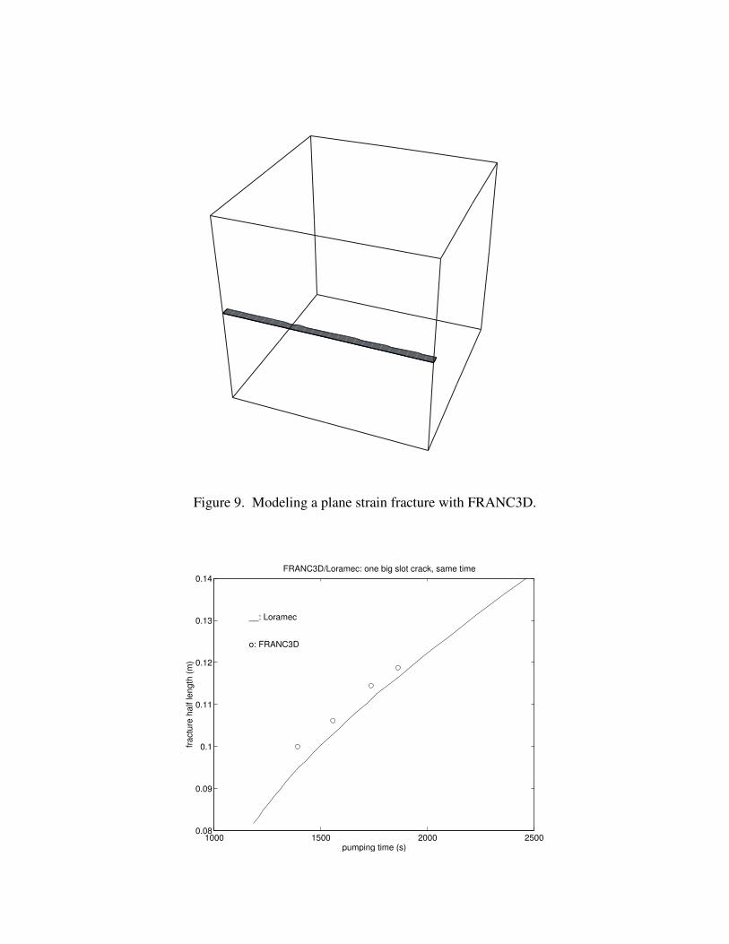
Figure 9. Modeling a plane strain fracture with FRANC3D.

1000 1500 2000 25000.08

0.09

0.1

0.11

0.12

0.13

0.14

pumping time (s)

fract

ure

half

leng

th (m

)

FRANC3D/Loramec: one big slot crack, same time

__: Loramec

o: FRANC3D

0 0.02 0.04 0.06 0.08 0.1 0.120

2

4

6

8

10

12

14

position of the nodes (m)

tota

l flu

id p

ress

ure

(MP

a)

FRANC3D/Loramec: one big slot crack, same length

*: Loramec

o: FRANC3D

0 0.02 0.04 0.06 0.08 0.1 0.120

1

2

3

4

5

6

7x 10−5

pumping time (s)

fract

ure

aper

ture

(m)

FRANC3D/Loramec: one big slot crack, same length

*: Loramec

o: FRANC3D

Figure 10. Comparison between FRANC3D and Loramec: plane strain case.

Figure 11. Modeling an axisymmetric fracture with FRANC3D.

o: FRANC3D

_: Loramec

0 50 100 150 200 2500.01

0.02

0.03

0.04

0.05

0.06

0.07

0.08

Pumping time (s)

Frac

ture

radi

us (m

)

FRANC3D/Loramec: radial, same time

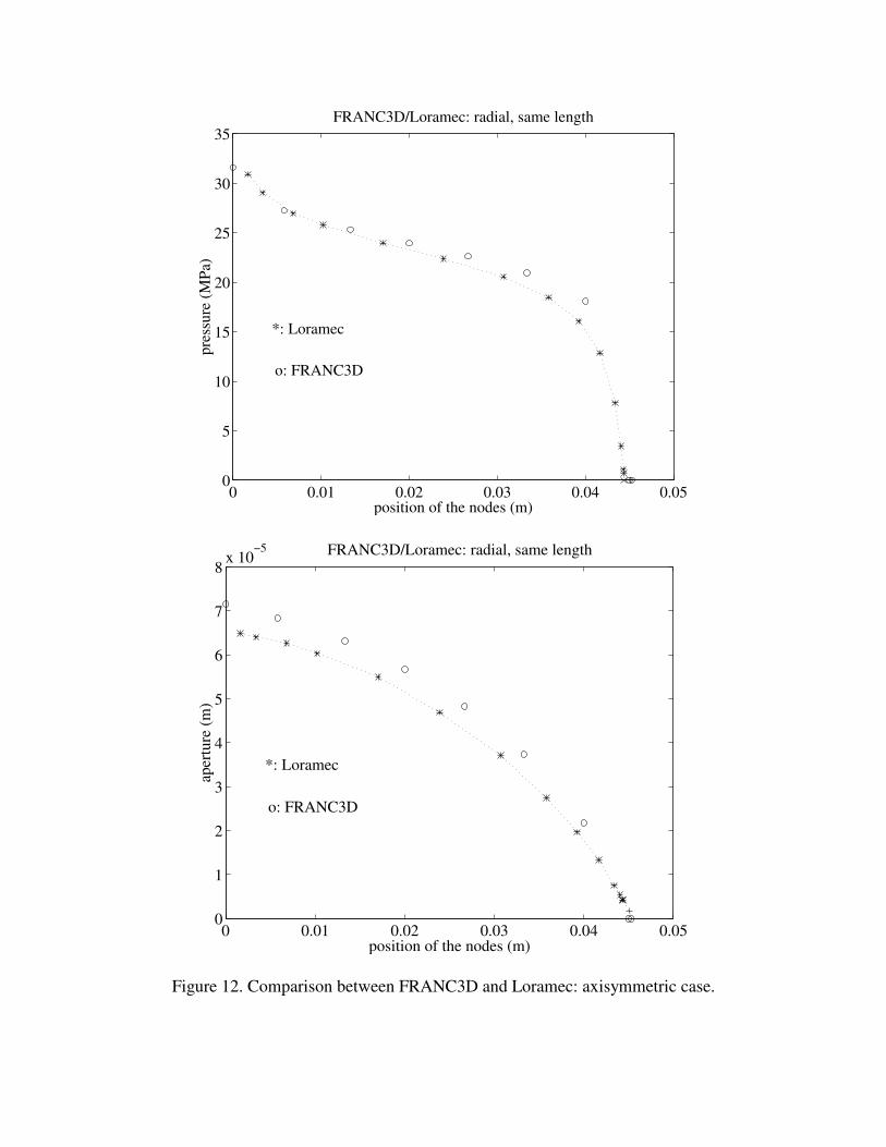
*: Loramec

o: FRANC3D

0 0.01 0.02 0.03 0.04 0.050

5

10

15

20

25

30

35

pres

sure

(MPa

)

position of the nodes (m)

FRANC3D/Loramec: radial, same length

*: Loramec

o: FRANC3D

0 0.01 0.02 0.03 0.04 0.050

1

2

3

4

5

6

7

8x 10

−5

aper

ture

(m)

position of the nodes (m)

FRANC3D/Loramec: radial, same length

Figure 12. Comparison between FRANC3D and Loramec: axisymmetric case.

Figure 13: Geometry of experiment COH10 (from Weijers, 1995).

2000 2200 2400 2600 2800 3000 3200 3400 3600 3800 40000

5

10

15

20

25

30

35

40

Experimental time (s0

Flui

d pr

essu

re (M

Pa)

PRES−COH10

__: experiment

o: FRANC3D

2000 2200 2400 2600 2800 3000 3200 3400 3600 3800 40000

5

10

15

20

25

30

35

40

45

50DIS2−COH10

Experimental time (s0

disp

lace

men

t (m

icro

ns)

__: experiment

o: FRANC3D

2000 2200 2400 2600 2800 3000 3200 3400 3600 3800 40000

5

10

15

20

25

30

35

40

45

50DIS3−COH10

Experimental time (s0

disp

lace

men

t (m

icro

ns)

__: experiment

o: FRANC3D

Figure 14: Comparison between FRANC3D and experiment COH10.