Simulating Biochemical Reaction Networks usingLattice Microbes: A Workflow

August 3rd, 2012

Piyush Labhsetwar, Elijah Roberts and Zaida Luthey-Schulten

Luthey-Schulten GroupUniversity of Illinois at Urbana-Champaign

http://www.scs.illinois.edu/schulten/http://latticemicrobes.sourceforge.net/

1 Rm

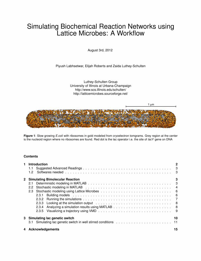
Figure 1: Slow growing E.coli with ribosomes in gold modeled from cryoelectron tomgrams. Grey region at the centeris the nucleoid region where no ribosomes are found. Red dot is the lac operator i.e. the site of lacY gene on DNA

Contents

1 Introduction 21.1 Suggested Advanced Readings . . . . . . . . . . . . . . . . . . . . . . . . . . . . . . . . . . . 31.2 Softwares needed . . . . . . . . . . . . . . . . . . . . . . . . . . . . . . . . . . . . . . . . . . 3

2 Simulating Bimolecular Reaction 32.1 Deterministic modeling in MATLAB . . . . . . . . . . . . . . . . . . . . . . . . . . . . . . . . . 32.2 Stochastic modeling in MATLAB . . . . . . . . . . . . . . . . . . . . . . . . . . . . . . . . . . 42.3 Stochastic modeling using Lattice Microbes . . . . . . . . . . . . . . . . . . . . . . . . . . . . 6

2.3.1 Building models . . . . . . . . . . . . . . . . . . . . . . . . . . . . . . . . . . . . . . . 62.3.2 Running the simulations . . . . . . . . . . . . . . . . . . . . . . . . . . . . . . . . . . . 72.3.3 Looking at the simulation output . . . . . . . . . . . . . . . . . . . . . . . . . . . . . . 82.3.4 Analyzing a simulation results using MATLAB . . . . . . . . . . . . . . . . . . . . . . . 82.3.5 Visualizing a trajectory using VMD . . . . . . . . . . . . . . . . . . . . . . . . . . . . . 9

3 Simulating lac genetic switch 103.1 Simulating lac genetic switch in well stirred conditions . . . . . . . . . . . . . . . . . . . . . . 11

4 Acknowledgements 15

1 Introduction

Lattice Microbes is a software package to carry out well-stirred and spatially resolved stochastic simulationsof biochemical reaction networks at whole cell level with realistic cytoplasmic crowding. Reaction networksare modeled in two popular frameworks, deterministic and stochastic. Deterministic modeling uses ordinarydi↵erential equations (ODE) while stochastic modeling uses the chemical master equation (CME). ODEframework assumes that amount of reacting species is a continuous variable which is true in case of largeconcentrations typically dealt in chemical laboratory but in biological systems, some species like DNA ortranscription factors are in very low copy number. Hence the assumption of continuity breaks and discreetnessin their amount needs to be accounted for which creates stochastic behavior. CME treats the chemical species’counts discreetly and samples them from probability distributions described by propensities for each of thereaction. CME framework assumes well-stirred conditions which means the reaction between two speciesis not di↵usion limited hence spatial information about their location is not taken into account. Biologicalsystems are not well-stirred environments with compartments and obstacles like ribosomes and large proteincomplexes. Reaction di↵usion master equation (RDME) accounts for the di↵usion of chemical species inspace and hence the spatial heterogeneity. RDME extends the CME formalism of the system to includespatial heterogeneity by dividing the space into discrete subvolumes, where particles di↵use in and out of asubvolume and react with particles only in its own subvolume, hence assuming well-stirred conditions in asubvolume. The RDME governs the time evolution of the probability, P , of a system being in a given statex (where the state is defined by the number active particles of each type in each subvolume of the system):

@P (x, t)

@t

=X

v2V

RX

r=1

�a

r

(xv

)P (x, t) + a

r

(xv

� S

r

)P (x� S

r

1v

, t)

+X

i2V

X

j2V

NX

↵=1

�d

↵

ij

x

↵

i

P (x, t) + d

↵

ji

(x↵

j

+ 1↵j

)P (x+ 1↵j

� 1↵i

, t)

Here, x↵

v

is the number of molecules of species ↵ (↵ = 1, · · · , N) in subvolume v (v 2 V ). R is the numberof reactions. a

r

is the reaction propensity for reaction r in given the state of a subvolume x

v

. S is thestoichiometry matrix. d↵

ij

is the di↵usive propensity for one molecule of species ↵ to di↵use from subvolumei to j. The first line on the right hand side governs reactivity between species in each subvolume; it is similarto the CME, in e↵ect assuming spatial homogeneity within each subvolume during each time step. Thesecond line on the right hand side governs di↵usivity into and out of each subvolume.

Lattice Microbes implement CME to simulate time evolution of biochemical system in well- stirredconditions and Reaction Di↵usion Master Equation (RDME) for spatially inhomogenous systems. Boththese equations are analytically intractable hence are studied by sampling the state of the system usingthese equations over time to generate large ensemble of trajectories. Lattice Microbes also implements anovel algorithm called Multiparticle Di↵usion Model-RDME (MPD-RDME). This is an approximate methodto sample RDME but it is highly parallelizable and hence is able take advantage of GPU for its acceleration.In this methodology, very short time steps are taken such that a particle doesn’t participate in more than onereaction and hence each subvolume can be independently simulated. Lattice Microbes have the capabilityto mimic realistic in vivo crowding conditions inside of a cell. Cytoplasmic crowding data obtained fromcryoeletron tomograms and proteomics experiments are used to categorize lattice sites or subvolumes asobstacles in which no particle can di↵use. Lattice microbes can simulate any biochemical reaction networkwhich has kinetic details and can be imported in SBML format, a popular file format.

It this workflow we will start with simulating a simple reversible bimolecular reaction deterministically andstochastically in well-stirred conditions in MATLAB to appreciate the di↵erences between the two frameworksand learn how to sample chemical master equation. Next we will use the Lattice Microbes to simulate 100di↵erent trajectories for the same bimolecular reaction in well-stirred conditions in a cell approximately thesize of E.coli. We will also simulate this reaction using RDME in an empty cubic cell modeled as 32*32*32subvolume lattice. At last we will simulate a complex biochemical reaction network called lac genetic switchin E.coli which exhibits bistability. The stochastic behavior of this genetic system generating heterogeneityin a clonal population (2 stable sub-populations) is perfectly captured only when treated within stochasticframework. Download the zip file LaticeMicrobesWorkflowFiles.zip containing Matlab codes needed for

analysis and output trajectories from here http://www.scs.illinois.edu/schulten/lm/index.html andextract it.

1.1 Suggested Advanced Readings

1. Stochastic simulation of reaction networks ”Stochastic simulation of chemical kinetics.” Daniel T Gille-spie, Annual review of physical chemistry,2007, 58, 35-55

2. Deterministic modelling and stochastic simulation of biochemical pathways using MATLAB M. Ullah,H. Schmidt, K.-H. Cho and O. Wolkenhauer, 2006 Systems Biology, IEEE Proceedings

3. Spatial stochastic modelling of the phosphoenolpyruvate-dependent phosphotranferase (PTS) pathwayin Escherichia coli J. Vidal Rodriguez, Jaap A Kaandorp, Maciej Dobrzynzki and Joke G. Blom, 2006,Bioinformatics

4. Multiple Particle Di↵usion model and software introduction:”Long time-scale simulations of in vivo di↵usion using GPU hardware” Elijah Roberts, John E. Stone,Leonardo Sepulveda, Wen-Mei W. Hwu and Zaida Luthey-Schulten, 2009 Proceedings of the 2009 IEEE

International Symposium on Parallel and Distributed Processing

5. Implementation of Lattice Microbes to study Lac genetic switch: ”Noise Contributions in an InducibleGenetic Switch: A Whole-Cell Simulation Study” Elijah Roberts, Andrew Magis, Julio O. Ortiz,Wolfgang Baumeister and Zaida Luthey-Schulten, 2011 PLoS Computational Biology, 7, e1002010

1.2 Softwares needed

1. Lattice Microbes (See instructions in user guide to use the binaries or compile locally) http://www.scs.illinois.edu/schulten/lm/index.html

2. MATLAB (Not 2012a [7.14], earlier version should work)

3. HDFView http://www.hdfgroup.org/hdf-java-html/hdfview/

4. VMD 1.9.1 (64 bit version) http://www.ks.uiuc.edu/Development/Download/download.cgi?PackageName=VMD Look under Uno�cial VMD builds for 64 bit mac version

2 Simulating Bimolecular Reaction

We will start with simulation of a simple bimolecular reaction to get you started with the concepts of reaction

kinetics and their stochastic simulation. Consider a reversible bimolecular reaction A+B

k1�*)�k2

C.

2.1 Deterministic modeling in MATLAB

In deterministic framework, concentration of chemical species is a variable whose evolution over time isstudied. For a generic set of reactions, we can write dC

dt

= S.v where C is concentration of species, S is thestoichiometric matrix containing coe�cients of metabolites for each reaction and v is the flux through thereactions. For the reaction above, we can write the ODEs for rate of change of concentrations of A,B and Cas follows

dCAdt

= k2CC

� k1CA

C

B

dCBdt

= k2CC

� k1CA

C

B

dCCdt

= k1CA

C

B

� k2CC

We will simulate this bimolecular reaction with k1 = 1.07x105M�1 s�1 and k2 = 0.351 s�1, initial counts of1000 for both A and B for 10 sec in a volume of 10�15 lit. This set of coupled ODE’s can be easily solvedin MATLAB using the following code [1]. This code can be found in bimolDeterministic.m file. :

k =⇥k1 k2

⇤

S =

2

4�1 1�1 11 �1

3

5

L =

2

41 01 00 1

3

5

initialCounts=[1000;1000;0];

V = 1e-15;

Na = 6.023e23;

initialConc = initialCounts./(V*Na);

S=[-1 1 ;-1 1 ;1 -1];

L=-S.*(S<0);

k=[1.07e5 0.351];

M1s=ones(size(k));

dC = @(t,x) S*(k.*prod(x(:,M1s).^L)).’;

[t,x]=ode15s(dC,[0:1e-3:10],initialConc);

x=x.*(V*Na);

hold on;

plot(t,x(:,1),’r’,’LineWidth’,2);

plot(t,x(:,2),’b’);

plot(t,x(:,3),’g’);

xlabel(’Time (sec)’,’FontSize’,20);

ylabel(’Particle Counts’,’FontSize’,20);

legend(’A’,’B’,’C’);

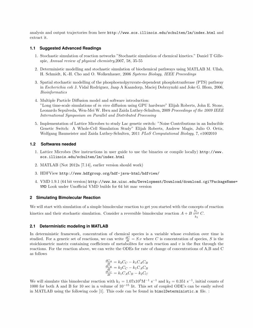
The plots of particle number with time show the decay in A and B and build up of C which reach theirsteady state in around 5 sec.

2.2 Stochastic modeling in MATLAB

In stochastic framework, we calculate the propensity for each reaction i.e how likely is a particular re-action to take place given the particle counts. For a unimolecular reaction A! with rate constant k1,propensity = k1 ⇤ PA

. For a bimolecular reaction A+B !, its given by propensity = k1V

⇤ PA

⇤ PB

and for

2A !, its given by propensity = k1V

⇤ PA⇤(PA�1)2 . Gillespie’s algorithm is used to sample the CME for 10

sec to generate a trajectory using following code. Note that we used the relationship between the stochasticand deterministic second order rate constants k2’ = k2/NA/V with a simulation volume of V = 1x10�15 Lto obtain the rate constant for the model. This code can be found in bimolStochastic.m file.

function enzkin stoch

S = [ -1 1

-1 1

1 -1

];

V = 1e-15;

Na = 6.023e23;

n0 = [1000;1000;0];

L = -S.*(S < 0);

tf = 10;

c=[1.78e-4 0.351];

runs = 1;

[ts,ns] = stoch(n0,c,S,L,tf);

hold on;

plot(ts,ns(1,:),’r’,’LineWidth’,3);

plot(ts,ns(2,:),’b’);

plot(ts,ns(3,:),’g’);

legend(’A’,’B’,’C’);

xlabel(’Time (sec)’,’FontSize’,20);

ylabel(’Particle count’,’FontSize’,20);

function varargout = stoch(varargin)

% % % N0: Column Vector of initial populations of all the species involved

% C: Row vector of stochastic rate constants of all elementary reactions

% S: Stoichiometry matrix with rows correspoding to species and columns

% corresponding to reaction channels

% L: Stoichiometry matrix for reactants only such that L = -D.*(D < 0);

% TF: Final time of simulation

% Ts: Row vector of time points of reaction events

% Ns: Matrix of output concentrations with a column for each time point.

args = varargin;

if nargin<6, args{6} = 1; end % single run by default

[n0,c,d,l,tf,runs] = args{:}; % parse inputs

oneszk = ones(size(c)); i1 = l==1; % reactions of type: A->B, A+B->AB

i2 = l==2; % reactions of type: A+A->AA

stop = tf - eps(tf); % simulation stop time

nOut = nargout;

% stochastic part:

if runs < 2 % single run

[yout{1:2}] = gillespie; % run gillispie

else % multiple runs

[tg,ng] = deal(cell(1,runs));

for i = 1:runs, [tg{i},ng{i}] = gillespie; end % run gillispie

yout = {tg,ng};if nOut>2

tt = unique([tg{:}]); % record times

numeltt = numel(tt); % record populations

nn = zeros(numel(n0), numeltt, runs);

for i = 1:numeltt

for j = 1:runs

id = find(tg{j} <= tt(i),1,’last’);

nn(:,i,j) = ng{j}(:,id);end

end

yout(3:4) = {tt,mean(nn,3)}; % append population mean

end

end

% Output:

varargout = yout;

% gillespie algorithm (direct method):

function [tt,nn] = gillespie;

t = 0; % initial time

n = n0; % initial population

tt = [];

nn = [];

rand(’state’, sum(100*clock)); % reset random number generator

while t <= stop

0 1 2 3 4 5 6 7 8 9 100

100

200

300

400

500

600

700

800

900

1000

Time (sec)

Parti

cle

Cou

nts

ABC

0 1 2 3 4 5 6 7 8 9 100

100

200

300

400

500

600

700

800

900

1000

Time (sec)

Parti

cle

coun

t

ABC

Figure 2: Left: Deterministic solution from Matlab, Right: One trajectory from stochastic solution in Matlab

tt = [tt t]; % record time

nn = [nn n]; % record population

m = n(:,oneszk); % replicate n : size(m,2) = size(k)

b = double( l); b(i1) = m(i1); % reactions of type: A->B, A+B->AB

b(i2) = m(i2).*(m(i2)-1)/2; % reactions of type: A+A->AA

a = c.*prod(b); % propensity

astr = sum(a); if astr, break, end % substrate utilised

tau = -1/astr*log(rand); % time to next reaction

u = find(cumsum(a)>astr*rand,1);% index of next reaction

n = n + d(:,u); % update population

t = t + tau; % update time

end

tt = [tt tf];

nn = [nn nn(:,end)];

end

end

end

2.3 Stochastic modeling using Lattice Microbes

We will simulate two variations of the bimolecular reaction, one in which the molecules are assumed tomove very quickly relative to the reaction rate (well-stirred) and one in which the di↵usion rates do playa significant role in the reacting system. We will solve these two models using chemical master equation(CME) and reaction-di↵usion master equation (RDME) sampling methods, respectively. The overall stepsinvolved will be as follows:

1. Build the simulation files containing the reaction and di↵usion models.

2. Run the simulations using any solver specific parameters.

3. Analyze the simulation output. Output is saved directly into the simulation file.

2.3.1 Building models

The most straightforward way to construct a reaction model for a Lattice Microbes simulation is to directlyset the matrices in the simulation file. The utilities lm setrm and lm setdm allow one to set the matricesfor the reaction and di↵usion models, respectively. The details of the matrices themselves will be describedelsewhere. we use the following command to build the reaction model:

[user@host qs/bimol] ./lm setrm bimol-cme.lm numberSpecies=3 numberReactions=2 "Initial \SpeciesCounts=[1000,1000,0]" "ReactionTypes=[2,1]" "ReactionRateConstants(:,0)= \[1.78e-4;0.351]" "StoichiometricMatrix=[-1,1;-1,1;1,-1]" "DependencyMatrix=[1,0;1,0;0,1]"

The file bimol-cme.lm is now ready to be simulated using the CME. Since the reaction portion of anRDME model is identical to the CME model, we simply copy the reaction model to a new simulation fileand then set the di↵usion matrices on the new file. Here, we use a di↵usion coe�cient D = 1x10�14

m

2s

�1

for all molecules and a 32x32x32 lattice with a spacing of 31.25x10�9m.

[user@host qs/bimol]$ cp bimol-cme.lm bimol-rdme.lm

[user@host qs/bimol]$ ./lm setdm bimol-rdme.lm numberReactions=2 numberSpecies=3 \numberSiteTypes=1 "latticeSize=[32,32,32]" latticeSpacing=31.25e-9 \particlesPerSite=8 "DiffusionMatrix=[1e-14]" "ReactionLocationMatrix=[1]"

The file bimol-rdme.lm is now ready to be simulated using the RDME.

2.3.2 Running the simulations

Sampling the CME using the Gillespie direct method

To simulate the well-stirred version of the bimolecular reaction model, we will use the Gillespie direct method,which is the default method for well-stirred simulations in Lattice Microbes. Before we run the simulations,we first set a few simulation parameters for the solver. The lm setp utility allows one to set solver specificparameters in the simulation file. Here, we tell the solver to simulate for 10 seconds and write out the systemstate every 0.001 second.

[user@host qs/bimol]$ ./lm setp bimol-cme.lm writeInterval=1e-3 maxTime=1e1

Finally, we run the actual simulation itself:

[user@host qs/bimol]$ ./lm -r 1-100 -ws -f bimol-cme.lm

The -r option tells the solver to simulate replicates 1-100 and the -ws option tells Lattice Microbes touse the default well-stirred solver. Following completion of the runs the bimol-cme.lm file will contain thesampling data for all of the simulation replicates.

Sampling RDME using the next-subvolume method

If no GPUs are attached to your computer, the only available RDME solver is the next-subvolume method.We first set the appropriate parameters as before, but additionally, since we wish to track individualmolecules, we must set a lattice output interval. Writing the lattice too frequently can consume an enormousamount of disk space so one should sample the lattice much less frequently than the system state, whichonly outputs the total count of each molecule type. Here, we sample the lattice every 0.1 second so we willhave 100 samples of each 10 second simulation replicate.

[user@host qs/bimol]$ ./lm setp bimol-rdme.lm writeInterval=1e-3 \latticeWriteInterval=1e-1 maxTime=1e1

We then run the RDME simulations. These simulations take significantly longer than the well-stirred equiv-alents, so here we only simulate 10 replicates:

[user@host qs/bimol]$ ./lm -r 1-10 -sl lm::rdme::NextSubvolumeSolver \-f bimol-rdme.lm

All of the system state information and lattice data for every replicate will be saved into the bimol-cme.lmfile.

2.3.3 Looking at the simulation output

The output data is stored in a Lattice Microbes simulation file, which is an HDF5 encoded file that storeslarge, independent data sets in a hierarchical structure. To view the data, one must use an HDF5 viewersuch as HDFView available at: http://www.hdfgroup.org/hdf-java-html/hdfview/.

Opening simulation file

To open a Lattice Microbes simulation file in HDFView choose File -> Open from the menu. Navigate toyour qs/bimol directory in the Open dialog. Be sure to change the Files of Type: option to All Filesand then select the bimol-cme.lm file. Once the file is opened, the individual folders containing the Model,Parameters, and Simulation data can be expanded. Datasets are shown as small grid-like icons underneaththe folders. Double clicking on a dataset will display its contents in the viewer panel to the right.

Overview of the file format

Lattice Microbes simulation files are organized into three top level folders: Model, Parameters, and Simu-lation. The Model folder contains two subfolders for the Reaction and Di↵usion models, as needed for thesim- ulation. Each folder has several attributes and contains several datasets corresponding to the matricesthat describe the model. Further details of the matrices themselves are provided elsewhere. The Parametersfolder acts as a collection point for solver specific parameters, which are set as attributes on the folder.Details of individual parameters are provided elsewhere. The Simulations folder contains the actual outputfrom the simulations. Beneath the folder is one folder for each simulation replicate, numbered accordingly.For each simulation replicate the data is stored in a variety of matrices and folders, which are specific to thesimulation method.

2.3.4 Analyzing a simulation results using MATLAB

The HDF5 file format used by the Lattice Microbes software can be directly read by Matlab, easing theanalysis of simulation data. Here, we will calculate the probability as a function of time for the systemto have a specific number of A molecules, i.e.,P

A

(t). We will use this probability density function (PDF)to calculate the mean and variance as a function of time. In Matlab navigate to the directory where thesimulation files are stored. First, we load the number of A molecules for each replicate at each time pointfrom the simulation file and transform the counts into a PDF. This code can be found in bimolcmeLM.m file.

inputFilename=’bimol-cme.lm’;

x=[0:1000];

numberReplicates=100;

species=1;

for R=[1:numberReplicates]

if R == 1

ts=cast(permute(hdf5read(inputFilename,...

sprintf(’/Simulations/%07d/SpeciesCountTimes’,R)),[2,1]),’double’);

Pt=zeros(size(x,2),size(ts,2));

end

counts=cast(permute(hdf5read(inputFilename,...

sprintf(’/Simulations/%07d/SpeciesCounts’,R)),[2,1]),’double’);

for ti=[1:size(ts,2)]

Pt(counts(ti,species)+1,ti)=Pt(counts(ti,species)+1,ti)+1;

end

end

Pt=Pt./numberReplicates;

Note that HDF5 files store data in row major format while Matlab stores data in column major format.In the above Matlab code, we used the permute(hdf5read(...),[2,1]) command to reorder the 2D matricesto column major format after the data was loaded. Next, we calculate the mean and variance from the P

A

(t):

E=zeros(1,size(ts,2));

V=zeros(1,size(ts,2));

for ti=[1:size(ts,2)]

E(ti)=sum(x’.*Pt(:,ti));

V(ti)=sum((power(x’-E(ti),2)).*Pt(:,ti));

end

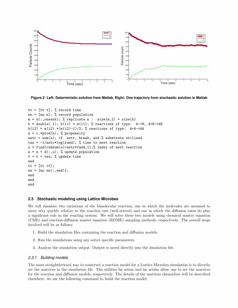
Finally, we plot the mean and variance as a function of time:

subplot(2,1,1);

plot(ts(1:10:end), E(1:10:end));

axis([0 10 1e2 1e3]); xlabel(’Time (s)’); ylabel(’E{A(t)}’);subplot(2,1,2);

plot(ts(1:10:end), V(1:10:end));

axis([0 10 1e0 2e2]); xlabel(’Time (s)’); ylabel(’Var{A(t)}’);

We can see that by taking average over 100 trajectories, the simulation output looks like the one fromdeterministic solution.

2.3.5 Visualizing a trajectory using VMD

You can use VMD to visualize RDME trajectories if LMplugin is installed. To install LMplugin copy thelmplugin.so file into plugins folder of VMD. Follow these instructions to do so.

(OS X) Copy the VMD plugin:[user@host /tmp]$ cp lm-2.0/lib/lmplugin.so \/Applications/VMD.app/Contents/vmd/plugins/MACOSXX86 64/molfile

(LINUX) Copy the VMD plugin:[user@host /tmp]$ cp lm-2.0/lib/lmplugin.so /usr/local/lib/vmd/plugins/LINUXAMD64/molfile

For general instructions on using VMD, please see the VMD help at http://www.ks.uiuc.edu/Research/vmd/. Here we will focus on using VMD to visualize Lattice Microbes trajectories.

Now open VMD and go to the menu and choose File->New Molecule.... Select Lattice Microbesin the Determine file type: drop down and browse to the file bimol-rdme.lm. Finally, press the Loadbutton.

The trajectory should load with 101 frames. Initially, the VMD OpenGL display will show only smallpoints for each molecule. Change the representation by choosing Graphics -> Representations... fromthe menu and then changing the Drawing Method drop down to be VDW. Now the molecules shouldappear as spheres. Next, change the Coloring Method drop down to be Type and molecules of di↵erenttypes should appear in di↵erent colors. Press the triangular play button to play the simulation trajectory.Finally, you may use the Selected Atoms text field in the Graphical Representations dialog to changewhich molecules are displayed. Change the text from ‘‘all’’ to ‘‘name particle and type 1’’ to showonly A molecules. Likewise you can use ‘‘name particle and type 2’’ and ‘‘name particle and type

3’’ to view molecules of type B and C respectively.

Figure 3: Mean (top) and Variance (bottom) for specie A over 100 trajectories

3 Simulating lac genetic switch

Lac genetic switch is an inducible genetic system used by E.coli to sense the presence of lactose and produceproteins to utilize it. This genetic system is used by E.coli to sense the presence of lactose and produceproteins to utilize it. It is known to exhibit bistability hence called a genetic switch. It behaves like a switchproducing two stable phenotypes, namely “un-induced state” exhibited in absence or low concentration ofexternal inducer (I

ex

) and “induced state” or “turned on” exhibited in presence of Iex

. Un-induced state ischaracterized by low copy number of LacY protein while induced cells have high copy number of LacY. I

ex

is sensed by cells when it is transported into the cytoplasm by LacY where it binds the lac repressor(R). Inabsence of I

ex

, R is bound to the operator site and hence represses the expression of genes in lac operon, oneof which is LacY. When I

ex

binds to R, it prevents it from binding to the operator site and hence allowingfor the expression of lac operon genes including LacY. Increased production of LacY transports more I

ex

tocytoplasm reducing the repression of lac operon which completes the positive feedback loop. For details onthis genetic system see Figure 5. We can represent all the processes in this genetic system by a set of 23biochemical reactions Figure 6. These reactions along with their rate laws and rate constants are stored infile called lac.sbml . You can find this file in LatticeMicrobesWorkflowFiles folder which you unzippedbefore to get Matlab codes. SBML is a popular format to encapsulate reactions along with their kineticinformation www.sbml.org. Lattice Microbes can import SBML files to be able to simulate any biochemical

Figure 4: Display of A (red), B (blue) and C (green) on a 32*32*32 lattice in VMD using the Lattice Microbe Plugin.

reaction system which follow simple rate laws like mass-action and hills-equation.

3.1 Simulating lac genetic switch in well stirred conditions

We will simulate the lac genetic switch for 10 hours which is the time taken for count of LacY proteinto stabilize. We will generate 100 di↵erent trajectories (replicates) each representing a unique cell in thepopulation. We will do this for four di↵erent inducer concentrations 10, 15, 20 and 30 µ M. At low inducerconcentration of 10 µ M, hardly any cell turns on (LacY<400-600). While at high inducer concentration of 30µ M, almost all cells turn on (LacY >1750). At intermediate I

ex

, we have 2 stable sub-populations of inducedand un-induced cells. We import the reaction network along with kinetic information from lac.sbml file. Tocarry out simulation using di↵erent initial concentrations of I

ex

, we will have to edit the sbml file whichspecifies the initial concentrations. Note that in this sbml file, the units used are particle number. Hencewe will have to calculate the corresponding particle number for the above mentioned concentrations usingAvogadro’s number and cell volume (8 x 10�16 lit) The particle numbers corresponding to I

ex

concentrationsof 10, 15, 20 and 30 µ M are 4816, 7224, 9632 and 14448 respectively. In the interest of time, we will changeboth external inducer concentration I

ex

and internal inducer concentration I to avoid the time taken for themto equilibriate. So you should have 4 files corresponding to 4 di↵erent concentrations of I

ex

. Note that if youuse same name for the lm file for di↵erent simulations, they will get appended by subsequent simulations soits better to name them di↵erently according to concentrations used. Here are commands for I

ex

=10 µM.You wil have to repeat this for other concentrations.

Importing lac sbml reaction model

Create a simulation file from the SBML file

[user@host qs/bimol]$ ./lm sbml import lac-cme-sbml 10.lm lac 10.sbml

LacY

LacIinducer

lac

RibosomemRNARNAP

A

B

C

D

E

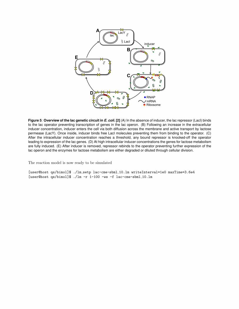
Figure 5: Overview of the lac genetic circuit in E. coli. [2] (A) In the absence of inducer, the lac repressor (LacI) bindsto the lac operator preventing transcription of genes in the lac operon. (B) Following an increase in the extracellularinducer concentration, inducer enters the cell via both diffusion across the membrane and active transport by lactosepermease (LacY). Once inside, inducer binds free LacI molecules preventing them from binding to the operator. (C)After the intracellular inducer concentration reaches a threshold, any bound repressor is knocked-off the operatorleading to expression of the lac genes. (D) At high intracellular inducer concentrations the genes for lactose metabolismare fully induced. (E) After inducer is removed, repressor rebinds to the operator preventing further expression of thelac operon and the enzymes for lactose metabolism are either degraded or diluted through cellular division.

The reaction model is now ready to be simulated

[user@host qs/bimol]$ ./lm setp lac-cme-sbml 10.lm writeInterval=1e0 maxTime=3.6e4

[user@host qs/bimol]$ ./lm -r 1-100 -ws -f lac-cme-sbml 10.lm

Table 1: Reactions and rate constants used in the stochastic model of the lac circuit

Reaction Param Stochastic Rate Units Sourcea Published in vitro Values Propensity

Lac operon regulation

R2 + O � R2O kron 2.43e+06 M�1s�1 M 4.0-20.0e+08b kronNAV · R2 · O

IR2 + O � IR2O kiron 1.21e+06 M�1s�1 M – kironNAV · IR2 · O

I2R2 + O � I2R2O ki2ron 2.43e+04 M�1s�1 M – ki2ronNAV · I2R2 · O

R2O � R2 + O kroff 6.30e-04 s�1 S 1.4-2.3e-02b kroff · R2OIR2O � IR2 + O kiroff 6.30e-04 s�1 S – kiroff · IR2OI2R2O � I2R2 + O ki2roff 3.15e-01 s�1 M – ki2roff · I2R2O

Transcription, translation, and degredation

O � O + mY ktr 1.26e-01 s�1 M – ktr · OmY � mY + Y ktn 4.44e-02 s�1 S – ktn · mYmY � � kdegm 1.11e-02 s�1 S – kdegm · mYY � � kdegp 2.10e-04 s�1 M – kdegp · Y

Lac inducer–repressor interactions TMG IPTG TMG IPTG TMG IPTG

I + R2 � IR2 kion 2.27e+04 9.71e+04 M�1s�1 M K – 9.2-9.8e+04c kionNAV · I · R2

I + IR2 � I2R2 ki2on 1.14e+04 4.85e+04 M�1s�1 M K – 4.6-4.9e+04c ki2onNAV · I · IR2

I + R2O � IR2O kiopon 6.67e+02 2.24e+04 M�1s�1 M K – 2.0-2.3e+04c kiopon

NAV · I · R2O

I + IR2O � I2R2O ki2opon 3.33e+02 1.12e+04 M�1s�1 M K – 1.0-1.2e+04c ki2opon

NAV · I · IR2O

IR2 � I + R2 kioff 2.00e-01 s�1 K 2.0e-01c kioff · IR2

I2R2 � I + IR2 ki2off 4.00e-01 s�1 K 4.0e-01c ki2off · I2R2

IR2O � I + R2O kiopoff 1.00e+00 s�1 K 0.5-1.0e+00c kiopoff · IR2OI2R2O � I + IR2O ki2opoff 2.00e+00 s�1 K 1.0-2.0e+00c ki2opoff · I2R2O

Inducer transport

Iex � I kid 2.33e-03 s�1 K 2.3e-03-1.4e-01d kid · Iex

I � Iex kid 2.33e-03 s�1 K 2.3e-03-1.4e-01d kid · I

Y + Iex � Y I kyion 3.03e+04 M�1s�1 K – kyion

NAV · Y · Iex

Y I � Y + Iex kyioff 1.20e-01 s�1 K – kyioff · Y IY I � Y + I kit 1.20e+01 s�1 K 1.2e+01e kit · Y IaS=in vivo single molecule experiment, K =in vitro (kinetic) experiment, M=model parameter fit to single-molecule distributionsb [92], c [74,75], d [69,93], e [70]

40

Figure 6: Reactions and rate constants used in the stochastic model of the lac circuit [2]

0 500 1000 1500 2000 2500 30000

10

20

30

40

50

60Iex = 10 microM

Num

ber o

f Cel

ls

0 500 1000 1500 2000 25000

10

20

30

40

50

60Iex = 15 microM

0 500 1000 1500 2000 2500 30000

10

20

30

40

50

60Iex = 20 microM

LacY copy number

Num

ber o

f Cel

ls

0 500 1000 1500 2000 2500 30000

10

20

30

40

50

60Iex = 30 microM

LacY copy number

Figure 7: Histograms of LacY copy number at the after 10 hours for different inducer concentrations

We can identify if a cell has turned on or not by finding the final copy number of LacY in the trajectories.We will make a histogram of the final copy number of LacY in 100 trajectories to observe the phenotypeof these 100 cells. You will see all cells are turned o↵ at I

ex

=10 µM while all are turned on at Iex

=30 µMbut at intermediate concentrations, of 15 µM and 20 µM, we see both phenotypes in the population whichpoints at bistability. All this code can be found in laccme.m file.

inputFilename=’lac-cme-sbml 10.lm’;

ts=cast(permute(hdf5read(inputFilename,sprintf(’/Simulations/%07d/SpeciesCountTimes’...

,1)),[2,1]),’double’);

numberReplicates=100;

finalLacY = zeros(numberReplicates,1);

for R=[1:numberReplicates]

counts=cast(permute(hdf5read(inputFilename,sprintf(’/Simulations/%07d/SpeciesCounts’...

,R)),[2,1]),’double’);

finalLacY(R) = counts(length(ts),9);

end

Repeat this step for 15, 20 and 30 µ M. hist(finalLacY);axis([0 3000 1e0 6e1]); xlabel(’LacY count number’); ylabel(’Number of Cells’);

4 Acknowledgements

Lattice Microbes development is supported by the Department of Energy O�ce of Science (BER) undergrant DE-FG02-10ER6510, National Science Foundation under grant NSF MCB 08-44670 and NSF Centerfor Physics of Living Cells.

References

[1] Ullah, M, Schmidt, H, Cho, K, Wolkenhauer, O (2006) Deterministic modelling and stochastic simulationof biochemical pathways using matlab. Systems biology 153:53–60.

[2] Roberts, E, Magis, A, Ortiz, JO, Baumeister, W, Luthey-Schulten, Z (2011) Noise contributions in aninducible genetic switch: A whole-cell simulation study. PLoS Comput. Biol. 7:e1002010.