Embed Size (px)
Citation preview

J Wetlands Biodiversity (2012) 2 21-35
Istros ndash Museum of Braila
SIMULATED TRANSPORT OF JET FUEL LEAKING INTO GROUND WATER SINDH PAKISTAN
Zulfiqar Ahmad Alan Fryar Mohsin Hafeez
Iftikhar Ahmad and Gulraiz Akhter Received 20042012 Accepted 18092012 Abstract A three-dimensional model of the contaminant transport was developed to predict the fate of jet fuel which leaked from the above surface storage tanks in the urban site of Karachi Pakistan Since the tanks were situated in a sandy layer the dissolved product entered the ground water system and started spreading beyond the site The modeling process comprised the steady-state simulation of the ground water system the transient simulation of the ground water system in the period from January 1986 through December 2073 and the calibration of jet fuel that was performed in context of different parameters in the groundwater system The fuel was simulated using a modular three-dimensional finite-difference groundwater model (PMWIN) ModFlow and a solute transport model (MT3D) in the 1986-2001 periods under a hypothetical scenario After a realistic distribution of piezometric heads within the aquifer system calibration was achieved and matched to known conditions the solute transport component was therefore coupled to the flow Jet fuel concentration contour maps show the expanding plume over a given time which becomes almost prominent in the preceding years Keywords calibration contaminant plume jet fuel Pakistan solute transport model Introduction1
Zulfiqar Ahmad and Gulraiz Akhter Department of Earth Sciences Quaid-i-Azam University Islamabad 45320 Islamabad Pakistan e-mail Zulfiqar Ahmad fz97hotmailcom Gulraiz Akhter agulraizhotmailcom Alan Fryar Deptartment of Earth and Environmental Sciences University of Kentucky 101 Slone Building Lexington KY 40506-0053 USA e-mail afryar1emailukyedu Mohsin Hafeez International Centre of Water for Food Security Charles Sturt University
Ground water is a major source for domestic and industrial uses in many urban settlements of the world Effluents from industrial areas as well as accidental spills and leaks from surface and underground storage tanks are the main sources of natural ground water contamination When such contamination is detected it becomes essential to estimate the spatial extent of contamination Conventionally determination of the extent of contamination is undertaken by collecting many samples within time and budgetary constraints from
Wagga Wagga NSW Australia e-mail mhafeezcsueduau Iftikhar Ahmad College of Earth and Environmental Sciences Punjab University Lahore Pakistan e-mail hydromodyahoocom
J Wetlands Biodiversity (2012) 2 21-35 22
several points which in general requires the installation of several observation wells As a result the cost of such operations can be very high especially when measurements with higher resolution are required
Two-dimensional (2-D) solute transport models can be used to predict the effects of transverse dispersion of the contaminant plume (spreading) Additionally 2-D models are appropriate where the contaminant source may lie within or near the radius of influence of a continuously pumping well While three-dimensional (3-D) numerical models should only be used if extensive data are available regarding vertical and horizontal heterogeneity and spatial variability in contaminant concentrations A localized contaminant transport model for groundwater is developed to gain insight into the dynamics of the leakage of jet fuel from above-ground storage tanks in the metropolitan area of Karcahi Pakistan The jet fuel consists of refined kerosene-type hydrocarbons which are mixtures of benzene toluene ethyl benzene and isomers of xylene (Kim and Corapcioglu 2003) Hypothetical monitoring wells were established to estimate the concentrations of jet fuel over a stipulated time period as a result of continuous seepage from the storage depot Although no specific data on the history of seepage were available in view of the results inferred from an electrical resistivity sounding survey (ERSS) coupled with the findings of previous investigators from (Mott MacDonald Pakistan [MMP] 2000) it is envisaged that seepage from the storage tanks occurred for more than a decade MMP 2000 conducted the study on soil and ground water assessment of environmental damage due to oil pollution and remedial measures were suggested for depots installations airfields of Shell Pakistan scattered throughout the country The Table 1 provides the composition of jet-fuel (Annexes) Literature Review
Kim and Corapcioglu (2003) developed a two-dimensional model to describe areal spreading and migration of light nonaqueous-phase liquids (LNAPLs) introduced into the subsurface by spills or leaks from underground storage tanks The nonaqueous-phase liquids (NAPL) transport model was coupled with two-dimensional contaminant transport models to predict contamination of soil gas and ground water resulting from a LNAPL migrating on the water table Simulations were performed using the finite-difference method to study LNAPL migration and ground water contamination The model was applied to subsurface contamination by jet-fuel Results indicated that LNAPL migration was affected mostly by volatilization Further the spreading and movement of the dissolved plume was affected by the geology of the area and the free-product plume Most of the spilled mass remained as a free LNAPL phase 20 years after the spill The migration of LNAPL for such a long period resulted in the contamination of both ground water and a large volume of soil
El-Kadi (2007) investigated the US Navys bulk fuel storage facility at Red Hill located on the island of Oahu The facility consisted of 20 buried steel tanks with a capacity of about 125 million gallons each The tanks contain jet-fuel and marine diesel fuel The bottoms of the tanks are situated about 80 feet above the basal water table The geology of the area is primarily basaltic lava flows Investigations found evidence of releases from several tanks Two borings were drilled to identify and monitor potential migration of contamination to the potable water source A numerical model of the regional hydrogeology at the Red Hill Fuel Storage Facility (RHFSF) was developed to simulate the fate and transport of potential contamination from the jet-fuel tanks and the effect on the saltwaterfreshwater transition zone of various pumping scenarios
Periago et al (2000) investigated infiltration into soil of contaminants present in cattle slurry Column experiments were performed in order to characterize the release
Istros ndash Museum of Braila
J Wetlands Biodiversity (2012) 2 21-35 23
of contaminants at the slurry-soil interface after surface application of slurry with subsequent rainfall or irrigation The shape of the release curves suggests that the release of substances from slurry can be modeled by a single-parameter release function They compared prediction of solute transport (a) with input defined by the release function and (b) assuming rectangular-pulse input
Eric et al (1986) developed a parameter identification (PI) procedure and implemented with the United States Geological Surveys Method of Characteristics (USGS-MOC) model The test results showed that the proposed algorithm could identify transmissivity and dispersivity accurately under ideal situations Because of the improved efficiency in model calibration the extended application to field conditions was effective
Jin et al (2008) investigated hydrocarbon plumes in ground water through the installation of extensive monitoring wells Electromagnetic induction survey was carried out as an alternative technique for mapping petroleum contaminants in the subsurface The surveys were conducted at a coal mining site near Gillette Wyoming using the EM34-XL ground conductivity meter Data from this survey used to validate with the known concentrations of diesel compounds detected in ground water Ground water data correlated perfectly with the electromagnetic survey data which was used to generate a site model to identify subsurface diesel plumes Results from this study indicated that this geophysical technique was an effective tool for assessing subsurface petroleum hydrocarbon sources and plumes at contaminated sites Materials and methods Site Description The project site is located between longitudes 67o 07prime 20Prime and 67o 10prime 30Prime and latitudes 24o 52prime 20Prime and 24o 54prime 20Prime The land surface elevation ranges from
approximately 50 to 109 ft (15 to 33 m) above mean sea level (AMSL) In the far south the Malir River drains into the Arabian Sea (Fig 1) The typical lithology of the site is silty to sandy clay from 0 to 15 ft (46 m) bls (below land surface) gravelly sand from 15 to 43 ft (46 to 13 m) bls and clayey to silty sand from 43 to 80 ft (13 to 24 m) bls The region is arid with an average annual rainfall of about 200 mm (79 in) Out of this only 10 (Arshaf and Ahmad 2008) is considered to recharge the aquifer system (634 x 10-9 msec)
The vadose zone is contaminated with up to 1300 ppm of total petroleum hydrocarbons (TPH) within the storage site In the previous study by (Mott MacDonald Pakistan [MMP] 2000) soil samples were collected from different locations with 3 feet (1 m) bls and analyzed to estimate the concentration of hydrocarbon compound Soil samples associated with the storage area have indicated higher TPH concentrations The contaminant plume follows the hydraulic gradient to the southwest Conceptual Model The groundwater flow system is treated as a two layer The upper layer (predominantly silty sand) is bounded above by the water table and is 15 ft (46 m) thick while the lower layer (predominantly clayey sand) is 65 ft (20 m) thick These are unconfined and recharged from the surface by infiltrating rain but only over permeable surfaces A small stream which runs along east of model area acts as a drain to groundwater which flows from the northeast to the southwest With the exception of the stream all other boundaries are artificial that is neither constant head nor constant flow boundaries The processes that control the groundwater flow are
(i) recharges from infiltrated rainfall
(ii) flow entering the model across the eastern boundary (also across the northern boundary)
(iii) flow reaching the stream
Istros ndash Museum of Braila
J Wetlands Biodiversity (2012) 2 21-35 24
(iv) flow leaving the model across the southern boundary and
pumping from one well near tank no 9
Figure no 1 Location of the study area
Values of hydraulic conductivities (K) for the layers are taken from the literature (Fetter 2000) The K value for depth range 16-31 ft (49-94m) is taken as 17x10-6 ftsec (52 x10-7 msec) and for depth range 31-97 ft (94-30 m) as 15x10-5 ftsec (46 x10-6
msec) The transport and fate of hydrocarbons
depend on multi-physical and chemical processes including advection dispersion volatilization dissolution biodegradation and sorption When a solute undergoes chemical reactions its rate of movement may be substantially less than the average rate of ground water flow In this study retardation of the movement of dissolved hydrocarbons is simulated as a sorption process which includes both adsorption and partitioning into soil organic matter or organic solvents
The MT3D software used for this simulation (Zheng 1990) uses a linear isotherm to simulate partitioning of a contaminant species between the porous media and the fluid phase due to sorption This sorption process is approximated by the following equilibrium relationship between the dissolved and adsorbed phases
S = KdC
Where S is the concentration of the adsorbed phase (MM) C is the concentration of the dissolved phase (ML3) and Kd is the sorption or distribution coefficient (L3M) Kd values for organic materials are commonly calculated as the product of the fraction of organic carbon in the soil foc and the organic carbon
Istros ndash Museum of Braila
J Wetlands Biodiversity (2012) 2 21-35 25
partitioning coefficient Koc or Kd = foc Koc Koc values are contaminant specific and reported in various sources (Key 1997 Jeng et al 1992 EPA 1989 ASTM 1995) The foc in the uncontaminated soil was estimated to range from 0001 to 002 based on guidance by Newell et al 1996 Assuming the linear isotherm the retardation factor (R) is expressed as follows
R = 1 + (rbneff) Kd
where rb is the bulk density of the porous material (ML3) and neff is the effective porosity
For jet fuel the distribution coefficient Kd is taken as 0004415 ft3kg With these values
R = 1 + [(48 kgft3)025] x 0004415 = 1848 (Kim and Corapcioglu 2003)
Numerical Ground Water Flow Modeling Processing ModFlow for Windows (PMWIN5) a modular 3-D finite-difference groundwater model is used to configure the flow field (McDonald and Harbaugh 1988) The model consists of 41 columns and 39 rows in each layer (Fig 2) The size of cells is 410 ft x 410 ft (125 m x 125 m) outside the fuel storage domain and 205 ft x 205 ft (625 m x 625 m) within the storage domain
Automatic calibration of the water table was made with algorithm - UCODE and a perfect match obtained with the known condition prior to developing the transport model (Poeter and Hill 1998 1999) Using the steady-state hydraulic heads calculated by PMWIN5 as the initial condition the solute transport model MT3D was run to simulate the dispersion of the dissolved jet-fuel plume (Zheng 1990)
The parameters adjusted were the retardation factor R for each cell within the finite-difference grid and the dispersion coefficient Concentration-time curves have been calculated for ten monitoring wells PMPATH (Chiang and Kinzelbach 1998) is used to retrieve the ground water flow model
and simulation result from PMWIN5 A semi-analytical particle-tracking scheme is used to calculate the ground water flow paths travel times and time-related capture zones resulting from pumping a neighboring well at the storage facility (Pollock 1989)
As a preprocessor to modeling and creating input data files the PMWIN5 utility package was used Prior to initiating the modeling work a ground water information system was established with all data in binary and or ASCII files that could be exported to other software Exploration Program (Hypothetical) The dissolved phase jet-fuel plume was traced using a combination of ten hypothetical monitoring wells (Fig 2) known as MW-1 through MW-10 The wells served to identify lithology observe water levels and monitor concentrations of organic compounds The wells extend to a depth of 80 ft (24 m) In addition the actual well was completed to a depth of 100 ft (305 m) near storage tank no9 in case of emergency need In the modeling study this well was used to track the time-related capture zone The general layout of the storage tanks over the finite-difference grid is shown in Fig 3 The location of the pumping well is marked as a small red square in Fig 2 and Fig 3 Model Calibration The model was calibrated for steady-state conditions Since it was speculated that the seepage of the fuel might have started as early as 1986 simulation of the ground water flow was begun in January 1971 the opening of storage facility In the steady-state phase the only input comes from constant head boundaries (along the east and west of the model) and from infiltrated rainfall
All output goes into constant head boundaries (the stream and the southwest boundary of the model) The differences in the known and simulated heads were calibrated to less than 030 ft (0091 m) by
Istros ndash Museum of Braila
J Wetlands Biodiversity (2012) 2 21-35 26
making slight adjustments in the K values of both layers
Figure no 2 Model design indicating finite difference grid and locations of hypothetical monitoring wells
Transient calibration of ground water
flow was accomplished using the time-variant hydraulic head values Parameters such as recharge rates during each stress period hydraulic heads in the stream and along with the model boundaries aquifer storage properties pumping rates and time-dependent capture zone were adjusted during the calibration
To be objective and consistent the recharge from infiltration was made equal to 10 of rainfall in each month Effective porosity of the aquifer was varied between
15 and 25 until the value of 25 was determined to be the best predictor for the model Constant pumping rates of 1500 US gallonshr (158 x 10-3 m3sec) and 1000 US gallonshr (105 x 10-3 m3sec) were used in layer 1 and layer 2 respectively
The period from 1986 through 2000 was divided into seven stress periods each of 2 years in duration From 2000 to 2001 one stress period was assigned The length of a stress period was made equal to the number of days in that month
Istros ndash Museum of Braila
J Wetlands Biodiversity (2012) 2 21-35 27
Figure no 3 Layout of the storage tanks marked on a finite-difference grid
Results and discussion
The effect of the pumping well is clearly visible as a cone of depression (Fig 4) The drawdown was determined to be 140 ft (43 m) near the storage facility Figure no 4 Cone of Depression visible around pumping well developed in layer 1
The model assumes uniform recharge from infiltrated rainfall to every ldquorechargingrdquo cell Although effective porosity hydraulic conductivity and recharge may vary in space and time the model is expected to have produced a reasonable configuration of the ground water flow pattern throughout the whole period of simulation The time-related capture zones produced due to constant pumping are shown in Figs 5 and 6 Water balances which was calculated for each year of the simulated period showed a perfect match between the input and output components Calibration of Plume Movement For simulation of the movement of dissolved jet fuel lateral hydraulic conductivity values equal to 0864 ftday (0263 mday) for layer 1 and 129 ftday (0393 mday) for layer 2 were accepted while the vertical hydraulic conductivity ones were taken as 00864 ftday (0263 mday) and 0129 ftday (0393 mday) for each layer respectively (Fetter
Istros ndash Museum of Braila
J Wetlands Biodiversity (2012) 2 21-35 28
2000) The hydraulic gradient and flow-net were obtained by running the flow component of the model derived from water level information in the previous study
The United States Environmental Protection Agency (USEPA) and the Georgia Environmental Protection Division (GAEPD) recommend that the value for longitudinal dispersion should be one-tenth of the distance from the place where a contaminant enters the ground water system to the down-gradient receptor (a well
stream or other point of compliance) The distance from the storage facility (tank no 7) to the pumping well is approximately 100 ft (3048 m) In all calibration runs as recommended the value for longitudinal dispersion was set at 10 ft (3 m) USEPA and GAEPD also recommend for a solute transport model that the value for transverse dispersion equal one-third of the longitudinal dispersion
Figure no 5 Capture zone of the pumping well with arrows indicating flow directions
For this model transverse dispersion would equal 33 ft (10 m) In the simulation of the fate of jet fuel the transverse dispersion coefficient was varied within a range of 20 ft to 33 ft (061 m to 10 m) In
the model a value of 0001ft2day (1 x 10⁻⁵ cm2sec) was used for molecular diffusion
With a retardation factor of 180 the dissolved jet fuel takes 133 years to travel a lateral distance of about 70 to 80 ft (21 to 24
Istros ndash Museum of Braila
J Wetlands Biodiversity (2012) 2 21-35 29
m) in ground water beneath tank no 8 The best value of the microbial decay coefficient for jet fuel is estimated to be 1-10 day with a
microbial yield coefficient for oxygen of 052 (Fetter 2000)
Figure no 6 500-day-capture zone calculated by PMPATH
Strategy Development for Release of Jet Fuel The previous integrity test run on the storage tanks containing 10 million litres of jet fuel indicated no loss The date when the leak initially began is unknown although inventory records indicated that the leak was not present before the tank integrity testing The product has been detected in several hypothetical-monitoring wells (notably in MW-2 and MW-4) and in many soil samples taken within several tens of feet of the tank (McDonald and Harbaugh 1988) The initial
concentration of jet fuel entering the system is not of prime concern for the modeling
The product of the influx (in L3T) and the concentration (in ML3) gives the total mass of jet fuel entering the system in a certain time interval For the purpose of calibrating the jet fuel input the initial concentration used based upon field data (Mott MacDonald Pakistan [MMP] 2000) varied from 0095 to 019 gft3 (00027 to 00054 gm3) The initial mass of jet fuel as simulated by the model was equal to each of four cells ldquoinjectingrdquo at a mass rate of 95 to 190 gft3 (27 to 54 gm3) following the
Istros ndash Museum of Braila
J Wetlands Biodiversity (2012) 2 21-35 30
initial period of 15 years during which no ground water contamination was assumed
(Tab 2)
Table no 2 Strategy developed for the plume modeling scenarios
Phase Stress period Condition Safe Period 15 years (1971 to 1986) No leakage Hazardous Period 10 years (1986 to 1996) Low to moderate leakage Risk Assessment 5 years (1996-2001) Moderate leakage Future Prediction 10 years (2001 ndash 2011) Accretion in leakage
Using steady-state hydraulic heads as initial conditions the evolution of the plume was modeled over nine stress periods as a result of continuous seepage from cells (18
16 1 tank 7) (19 16 1 tank 10) (19 17 1 tank 8) and (20 17 1 tank 9) as shown in Table 3
Table no 3 Stress period used in time-dependent solute transport modeling of jet fuel
Stress Period Time interval (years)
Elapsed Time (secs)
Period
1 2 630 x 107 1986 - 88 2 2 1260 x 107 1988 - 90 3 2 1892 x 107 1990 - 92 4 2 2523 x 107 1990 - 94 5 2 315 x 108 1994 - 96 6 2 378 x 108 1996 - 98 7 2 441 x 108 1998 - 00 8 1 473 x 108 2000 - 01 9 10 274 x 109 2001 - 11
Calibration Scenario
Parameters describing various processes are used after calibration with different combination of parameters (Tab 4)
The release of the jet fuel is simulated in four cells all along columns 18 to 20 from row 16 to row 17 The area of injection is equal to 42025 ft2 (3904 m2)
The concentration of jet fuel at the source (95 to 190 mgft3 [27 to 54 gm3]) maintained constant throughout the designated ldquohazardous periodrdquo simulation period (1986-1996) The concentration was
slightly increased (about 001 ) from 1996 through 2001 and further up to longer time duration of 10 years ie 2011 The plume simulations are shown in Fig 7 The jet-fuel break-through curves for the hypothetical monitoring wells are shown in Fig 8 Conventionally determination of the extent and level of contamination is undertaken by taking multiple measurements in wells (Zhou 1996 Plus and Paul 1997 Fisher and Goodman 2002) However higher spatial resolution generally requires installation of monitoring wells which is costly (Zeru 2004)
Istros ndash Museum of Braila
J Wetlands Biodiversity (2012) 2 21-35 31
Table no 4 Preliminary and final values of parameters used in modeling
Parameters Value Longitudinal Dispersion 10 ft Transverse Dispersion 33 ft Molecular Diffusion 0001 ft2day Distribution Coefficient 0004415 ft3kg Retardation Factor (R) 180 to 1848 Decay Coefficient 1 x10⁻⁹ day--1 Hydraulic Conductivity K (Layer-1) 1x10⁻⁵ ftsec (0864 ftday) Hydraulic Conductivity K (Layer-2) 149x10-5 ftsec (129 ftday) Effective Porosity (Layer-1) 025 Effective Porosity (Layer-2) 030
Figure no 7 Simulated Jet-fuel plumes (1986 to 1988 and 1988 to 1990)
Figure no 8 Concentration versus time based on data from 10 monitoring wells
The modeled concentration at MW-1 MW-2 and MW-6 was much higher than the concentrations in the remaining wells The maximum level of concentrations recorded in MW-6 was 2990 μgft3 Fig 9 reflects the plume spreading of year 2001
The shape of the plume is elliptical with the major axis in the direction of ground water flow This shape results from advection and longitudinal dispersion The lateral spread of the plume results from transverse dispersion and molecular diffusion The upgradient spread of the plume results from molecular diffusion (Bauer et al 2004 Bockelmann 2003) The
Istros ndash Museum of Braila
J Wetlands Biodiversity (2012) 2 21-35 32
plume travels toward the stream which is still far away in the west Figure no 9 Extent of simulated plume in 2001
By the end of 2011 the effect of the
plume becomes evident and the monitoring wells MW-4 MW-5 and MW-6 indicated increased concentration of jet fuel (Fig 10) The resultant plume appears to be spreading more in the elliptical path but in the direction of ground water flow Figure no 10 Extent of plume spreading in year 2011
Conclusions Based on the modeling it is concluded that the jet-fuel plume has neither expanded nor moved considerably It is less than 250 ft (762 m) beyond the storage tanks and is oriented northeast to southwest The level of concentration found in the simulated monitoring wells is significant but because ground water is brackish and thus unlikely to be used no harmful effects are expected An interdisciplinary investigation of the processes controlling the fate and the transport of hydrocarbons in the subsurface is needed
Concentrations should be performed in wells within and down-gradient of the plume as field data would help develop a stronger argument for the fate of jet fuel in ground water Rezumat
SIMULAREA TRANSPORTULUI DE COMBUSTIBIL SCURS IcircN APA
FREATICĂ IcircN ZONA SINDH PAKISTAN Un model tri-dimensional al transportului de poluanţi a fost dezvoltat pentru a prevede soarta jetului de combustibil care se scurge de la rezervoarele de stocare de suprafață din zona urbană din Karachi Pakistan Din momentul cacircnd tancurile au fost plasate icircntr-un strat de nisip produsul dizolvat a intrat icircn sistemul apelor subterane şi a icircnceput răspacircndirea dincolo de zona Procesul de modelare cuprinde simularea stării de echilibru a sistemului de apă freatică simularea tranzitorie a sistemului de apă freatică icircn perioada ianuarie 1986 pacircnă icircn decembrie 2073 precum şi calibrarea jetului de combustibil care a fost realizat icircn cadrul unor parametri diferiţi din apele subterane ale sistemului Combustibilul a fost simulat folosind un model modular tri-dimensional pentru apele subterane (PMWIN) ModFlow şi un model de transport al soluției (MT3D) icircn perioada 1986-2001 icircn cadrul unui scenariu ipotetic După o distribuție realistă a
Istros ndash Museum of Braila
J Wetlands Biodiversity (2012) 2 21-35 33
capetelor piezometrice icircn cadrul sistemului acvifer calibrarea a fost realizată şi adaptată la condițiile cunoscute componenta de transport a soluţiei a fost cuplată la curgere Hărţile de contur a concentraţiei jetului de combustibil arată expansiunea penei icircntr-un interval de timp dat care devine aproape proeminentă icircn anii precedenți Acknowledgments Austraining International and the Department of Education Employment and Workplace Relations (DEEWR) are gratefully acknowledged to provide post-selection support services and funding the research under the executive endeavour award 2010 Lauren Fyfe case manager of Austraining Sue Kendall and Umair Rabbani of the International Centre of Water for Food Security (IC Water) Charles Sturt University Wagga Wagga NSW Australia are acknowledged with thanks for timely support and provision of the essentials of research References ASHRAF A AHMAD Z (2008) Regional
groundwater flow modeling of upper Chaj Doab Indus Basin Geophysical Journal International (GJI) 173 17ndash24 doi101111j1365-246X200703708x
ASTM (1995) Standard Guide for Risk-Based Corrective Action Applied at Petroleum Release Sites American Society for Testing and Materials ASTM E-1739-95 Philadelphia PA
BAUER S BAYER-RAICH M HOLDER T KOLESAR C MULLER D PTAK T (2004) Quantification of groundwater contamination in an urban area using integral pumping tests JContam Hydrol 75 183-213
BOCKELMANN A ZAMFIRESCU Z PTAK T GRATHWOHL P TEUTSCH G (2003) Quantification of mass fluxes and natural attenuation rates at an industrial site with a limiten monitoring network a case study site J Contam Hydrol 60 97-121
CHIANG WH KINZELBACH IW (1998) PMPATH Processing Modflow and Modflow
EL-KADI A (2007) Groundwater Modeling Services for Risk Assessment Red Hill Fuel Storage Facilities NAVFAC Pacific Oahu Hawaii
EPA (1989) Determining Soil Response Action Levels Based on Potential Contaminant Migration to Ground Water A Compendium of Examples EPA5402-89057 October 1989
ERIC W STRECKER EW CHU W (1986) Parameter Identification of a Ground-Water Contaminant Transport Model Groundwater Vol 24 Issue 1 p 56-62
FETTER CW (2000) Applied hydrogeology (4t edition) Prentice Hall 598 pp
FISHER RS GOODMANN PT (2002) Characterizing groundwater quality in Kentucky from site selection to published information Proceedings of 2002 National Monitoring Conference National Water Quality Monitoring Council May 19-23 Madison Wisconsin
JENG CY CHEN DH YAWS CL (1992) Data Compilation for Soil Sorption Coefficient Pollution Engineering June 15 1992 p 54-60
JIN S FALLGREN P COOPER J MORRIS J URYNOWICZ M (2008) Assessment of diesel contamination in groundwater using electromagnetic induction geophysical techniques Journal of Environmental Science and Health Volume 43 Issue 6 May 2008 p 584ndash588
KEY (1997) Groundwater Fate and Transport Evaluation Report South Cavalcade Superfund Site Houston Texas prepared by KEY Environmental Inc on behalf of Beazer East Inc for the U S Environmental Protection Agency March 1997
KIM J CORAPCIOGLU MY (2003) Modeling dissolution and volatilization of LNAPL sources migrating on the groundwater table Journal of Contaminant Hydrology Vol 65 Issue 1-2 p 137-158
McDONALD MG HARBAUGH AW (1988) ModFlow A modular three-dimensional finite-difference ground-water flow model US Geological Survey Open-File Report 83-875 Chapter A1 Washington DC
MOTT McDONALD PAKISTAN (pvt) Ltd (2000) A report on soil and groundwater Assessment of depotsinstallationsairfields Shell Pakistan Limited
NEWELL C J MCLEOD RK GONZALES JR (1996) BIOSCREEN Natural
Istros ndash Museum of Braila
J Wetlands Biodiversity (2012) 2 21-35 34
Attenuation Decision Support System Userrsquos Manual Version 13 EPA600R-96087 National Risk Management Research Laboratory Office of Research and Development U S Environmental Protection Agency Cincinnati 45268 Ohio August 1996
PERIAGO EL DELGADO AN DIAZ-FIERROS F (2000) Groundwater contamination due to cattle slurry modeling infiltration on the basis of soil column experiments Water Research Vol 34 Issue 3 p 1017-1029
PLUS RW PAUL CJ (1997) Multi-layer sampling in conventional monitoring wells for improved estimation of vertical contaminant distribution and mass J Contam Hydrol 25 85-111
POETER EP HILL MC (1998) Documentation of UCODE a computer code for universal inverse modelling US Geological Survey Water-Resources Investigations Report 98-4080 Denver Colorado p 1-116
POETER EP HILL MC (1999) UCODE a computer modelling Computers amp Geosciences 25 457-462
POLLOCK DW (1989) Documentation of a computer program to compute and display path lines using results from the US Geological Survey modular three-dimensional finite-difference groundwater flow model US Geological Survey open-file report 89-381 Denver
ZHOU Y (1996) Sampling frequency for monitoring the actual state of groundwater systems J Hydrol 180 301ndash318
ZERU A (2004) Investigations numeacuteriques sur linversion des courbes de concentration issues dun pompage pour la quantification de la pollution de leau souterraine Numerical investigations on the inversion of pumped concentrations for groundwater pollution quantification PhD Thesis Universiteacute Louis Pasteur (France) 192 pp
ZHENG C (1990) MT3D A Modular Three-Dimensional Transport Model for Simulation of Advection Dispersion and Chemical Reactions of Contaminants in Groundwater Systems prepared for the U S Environmental Protection Agency Robert S Kerr Environmental Research Laboratory Ada Oklahoma 163 pp
Annexes Composition of Contaminant (Jet fuel) Knowledge of the geochemistry of a contaminated aquifer is important to understand the chemical and biological processes controlling the migration of hydrocarbon contaminants in the subsurface Originally the jet fuel (kerosene oil) is the name assigned to a material with a biological origin but now it is used to describe materials most of which contain carbon and hydrogen and which may contain oxygen nitrogen the halogens and lesser amounts of other elements The simplest of these are the hydrocarbons molecules of hydrogen and carbon many of which are the components of natural gas petroleum and coal Petroleum however has a very large number of components ranging from methane to the high molecular weight materials asphalt and paraffin Typical fractions into which crude oil is separated in an oil refinery and some principal molecular species are shown in Table 1
Istros ndash Museum of Braila
J Wetlands Biodiversity (2012) 2 21-35 35
Table no 1 The Fractions and Representative Components obtained from Crude Oil
Fraction from distillation
Boiling range Product of secondary treatment
Typical molecular components
Gas Below 20 oC Gas Liquefied Pet Gas (LPG)
CH4 methane C2H6 ethane C3H8 propane C4H10 butane
Naphtha 20 - 175 oC Naphtha gasoline C11H24 to C18H38 Kerosene 175 - 400 oC Kerosene diesel fuel C11H24 to C18H38 Lubricating oil C15H32 to C40H82 Residue above 400 oC Asphalt Heavier hydrocarbons
Istros ndash Museum of Braila
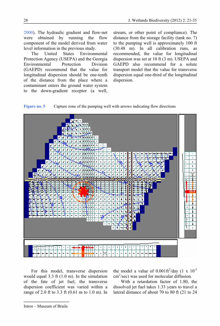