Embed Size (px)
Citation preview
1. Introduction2. Regression with a Single Predictor3. A Straight Line Regression Model4. The Method of Least Squares5. The Sampling Variability of the Least Squares
Estimators—Tools for Inference6. Important Inference Problems7. The Strength of a Linear Relation8. Remarks about the Straight Line Model Assumptions9. Review Exercises
11
Regression Analysis ISimple Linear Regression
45688_11_p429-474 7/25/05 9:57 AM Page 429

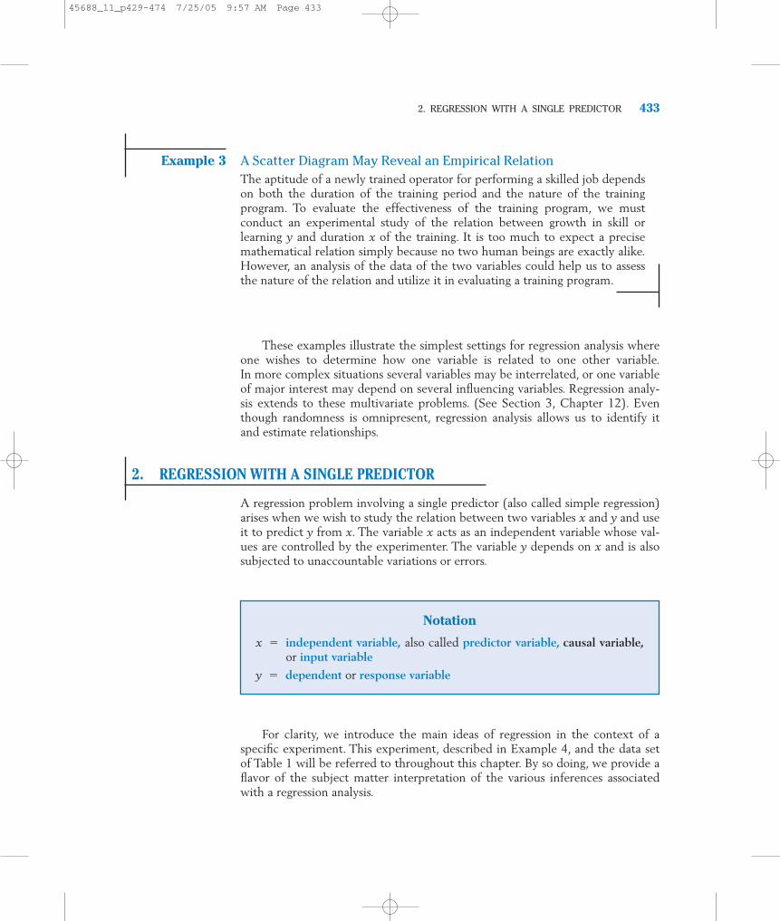
The Highest Roller Coasters are FastestSome roller coasters are designed to twist riders and turn them upside down.Others are designed to provide fast rides over large drops. Among the 12 tallestroller coasters in the world, the maximum height (inches) is related totop speed (miles per hour). Each data point, consisting of the pair of values(height, speed), represents one roller coaster. The fitted line predicts an increasein top speed of .17 miles per hour for each foot of height, or 17 miles per hourfor each 100 feet in height.
120
110
100
90
80
70
200 250 300 350 400
Spe
ed
Height
Fitted Line PlotSpeed � 39.06 � 0.1707 Height
© Rafael Macia/Photo Researchers, Inc.
45688_11_p429-474 7/27/05 3:07 PM Page 430

1. INTRODUCTION
Except for the brief treatment in Sections 5 to 8 of Chapter 3, we havediscussed statistical inferences based on the sample measurements of a singlevariable. In many investigations, two or more variables are observed for eachexperimental unit in order to determine:
1. Whether the variables are related.
2. How strong the relationships appear to be.
3. Whether one variable of primary interest can be predicted from obser-vations on the others.
Regression analysis concerns the study of relationships between variableswith the object of identifying, estimating, and validating the relationship. Theestimated relationship can then be used to predict one variable from the valueof the other variable(s). In this chapter, we introduce the subject with specificreference to the straight-line model. Chapter 3 treated the subject of fitting aline from a descriptive statistics viewpoint. Here, we take the additional step ofincluding the omnipresent random variation as an error term in the model.Then, on the basis of the model, we can test whether one variable actually influ-ences the other. Further, we produce confidence interval answers when usingthe estimated straight line for prediction. The correlation coefficient is shown tomeasure the strength of the linear relationship.
One may be curious about why the study of relationships of variables hasbeen given the rather unusual name “regression.” Historically, the word regressionwas first used in its present technical context by a British scientist, Sir Francis Gal-ton, who analyzed the heights of sons and the average heights of their parents.From his observations, Galton concluded that sons of very tall (short) parentswere generally taller (shorter) than the average but not as tall (short) as theirparents. This result was published in 1885 under the title “Regression TowardMediocrity in Hereditary Stature.” In this context, “regression toward mediocrity”meant that the sons’ heights tended to revert toward the average rather thanprogress to more extremes. However, in the course of time, the word regressionbecame synonymous with the statistical study of relation among variables.
Studies of relation among variables abound in virtually all disciplines of sci-ence and the humanities. We outline just a few illustrative situations in order tobring the object of regression analysis into sharp focus. The examples progressfrom a case where beforehand there is an underlying straight-line model that ismasked by random disturbances to a case where the data may or may not revealsome relationship along a line or curve.
Example 1 A Straight Line Model Masked by Random DisturbancesA factory manufactures items in batches and the production manager wishesto relate the production cost y of a batch to the batch size x. Certain costsare practically constant, regardless of the batch size x. Building costs and
1. INTRODUCTION 431
45688_11_p429-474 7/25/05 9:57 AM Page 431

administrative and supervisory salaries are some examples. Let us denote thefixed costs collectively by F. Certain other costs may be directly proportionalto the number of units produced. For example, both the raw materials andlabor required to produce the product are included in this category. Let Cdenote the cost of producing one item. In the absence of any other factors,we can then expect to have the relation
In reality, other factors also affect the production cost, often in unpredictableways. Machines occasionally break down and result in lost time and addedexpenses for repair. Variation of the quality of the raw materials may also causeoccasional slowdown of the production process. Thus, an ideal relation can bemasked by random disturbances. Consequently, the relationship between y andx must be investigated by a statistical analysis of the cost and batch-size data.
Example 2 Expect an Increasing Relation But Not Necessarily a Straight LineSuppose that the yield y of tomato plants in an agricultural experiment is tobe studied in relation to the dosage x of a certain fertilizer, while other con-tributing factors such as irrigation and soil dressing are to remain as constantas possible. The experiment consists of applying different dosages of the fer-tilizer, over the range of interest, in different plots and then recording thetomato yield from these plots. Different dosages of the fertilizer will typicallyproduce different yields, but the relationship is not expected to follow a pre-cise mathematical formula. Aside from unpredictable chance variations, theunderlying form of the relation is not known.
y � F � Cx
432 CHAPTER 11/REGRESSION ANALYSIS I
Regression analysis allows us to predict one variable from the value of another variable.(By permission of Johnny Hart and Field Enterprises, Inc.)
45688_11_p429-474 7/25/05 9:57 AM Page 432
Example 3 A Scatter Diagram May Reveal an Empirical RelationThe aptitude of a newly trained operator for performing a skilled job dependson both the duration of the training period and the nature of the trainingprogram. To evaluate the effectiveness of the training program, we mustconduct an experimental study of the relation between growth in skill orlearning y and duration x of the training. It is too much to expect a precisemathematical relation simply because no two human beings are exactly alike.However, an analysis of the data of the two variables could help us to assessthe nature of the relation and utilize it in evaluating a training program.
These examples illustrate the simplest settings for regression analysis whereone wishes to determine how one variable is related to one other variable.In more complex situations several variables may be interrelated, or one variableof major interest may depend on several influencing variables. Regression analy-sis extends to these multivariate problems. (See Section 3, Chapter 12). Eventhough randomness is omnipresent, regression analysis allows us to identify itand estimate relationships.
2. REGRESSION WITH A SINGLE PREDICTOR
A regression problem involving a single predictor (also called simple regression)arises when we wish to study the relation between two variables x and y and useit to predict y from x. The variable x acts as an independent variable whose val-ues are controlled by the experimenter. The variable y depends on x and is alsosubjected to unaccountable variations or errors.
For clarity, we introduce the main ideas of regression in the context of aspecific experiment. This experiment, described in Example 4, and the data setof Table 1 will be referred to throughout this chapter. By so doing, we provide aflavor of the subject matter interpretation of the various inferences associatedwith a regression analysis.
2. REGRESSION WITH A SINGLE PREDICTOR 433
Notation
x � independent variable, also called predictor variable, causal variable,or input variable
y � dependent or response variable
45688_11_p429-474 7/25/05 9:57 AM Page 433

Example 4 Relief from Symptoms of Allergy Related to DosageIn one stage of the development of a new drug for an allergy, an experimentis conducted to study how different dosages of the drug affect the duration ofrelief from the allergic symptoms. Ten patients are included in the experi-ment. Each patient receives a specified dosage of the drug and is asked toreport back as soon as the protection of the drug seems to wear off. Theobservations are recorded in Table 1, which shows the dosage x and durationof relief y for the 10 patients.
Seven different dosages are used in the experiment, and some of theseare repeated for more than one patient. A glance at the table shows that ygenerally increases with x, but it is difficult to say much more about the formof the relation simply by looking at this tabular data.
For a generic experiment, we use n to denote the sample size or the numberof runs of the experiment. Each run gives a pair of observations (x, y) in whichx is the fixed setting of the independent variable and y denotes the correspond-ing response. See Table 2.
We always begin our analysis by plotting the data because the eye can easilydetect patterns along a line or curve.
434 CHAPTER 11/REGRESSION ANALYSIS I
TABLE 1 Dosage x (in Milligrams) and the Number of Days of Relief yfrom Allergy for Ten Patients
Dosage Duration of Reliefx y
3 93 54 125 96 146 167 228 188 249 22
45688_11_p429-474 7/25/05 9:57 AM Page 434
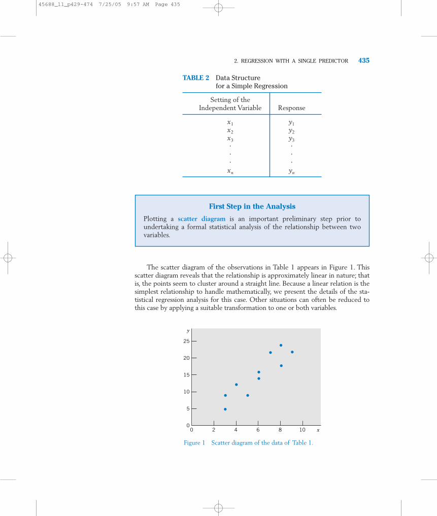
The scatter diagram of the observations in Table 1 appears in Figure 1. Thisscatter diagram reveals that the relationship is approximately linear in nature; thatis, the points seem to cluster around a straight line. Because a linear relation is thesimplest relationship to handle mathematically, we present the details of the sta-tistical regression analysis for this case. Other situations can often be reduced tothis case by applying a suitable transformation to one or both variables.
2. REGRESSION WITH A SINGLE PREDICTOR 435
First Step in the Analysis
Plotting a scatter diagram is an important preliminary step prior toundertaking a formal statistical analysis of the relationship between twovariables.
0
25
y
20
15
10
5
02 4 6 8 10 x
Figure 1 Scatter diagram of the data of Table 1.
TABLE 2 Data Structure for a Simple Regression
Setting of theIndependent Variable Response
x1 y1x2 y2x3 y3� �� �� �
xn yn
45688_11_p429-474 7/25/05 9:57 AM Page 435
3. A STRAIGHT LINE REGRESSION MODEL
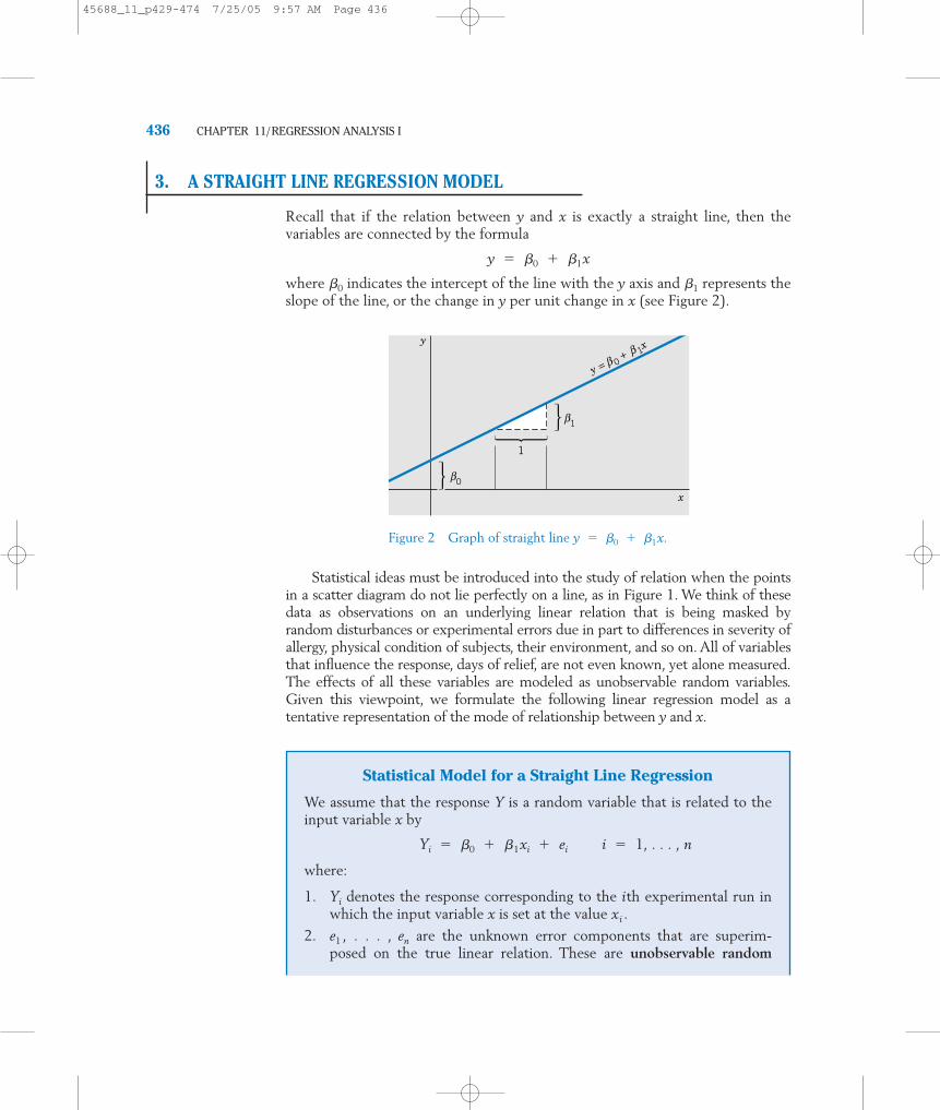
Recall that if the relation between y and x is exactly a straight line, then thevariables are connected by the formula
where �0 indicates the intercept of the line with the y axis and �1 represents theslope of the line, or the change in y per unit change in x (see Figure 2).
Statistical ideas must be introduced into the study of relation when the pointsin a scatter diagram do not lie perfectly on a line, as in Figure 1. We think of thesedata as observations on an underlying linear relation that is being masked byrandom disturbances or experimental errors due in part to differences in severity ofallergy, physical condition of subjects, their environment, and so on. All of variablesthat influence the response, days of relief, are not even known, yet alone measured.The effects of all these variables are modeled as unobservable random variables.Given this viewpoint, we formulate the following linear regression model as atentative representation of the mode of relationship between y and x.
y � �0 � �1x
436 CHAPTER 11/REGRESSION ANALYSIS I
1
β0
β1
x
y
y =
x
0β + 1β
Figure 2 Graph of straight line y � �0 � �1x.
Statistical Model for a Straight Line Regression
We assume that the response Y is a random variable that is related to theinput variable x by
where:
1. Yi denotes the response corresponding to the ith experimental run inwhich the input variable x is set at the value xi .
2. e1 , . . . , en are the unknown error components that are superim-posed on the true linear relation. These are unobservable random
Yi � �0 � �1xi � ei i � 1, . . . , n
45688_11_p429-474 7/25/05 9:57 AM Page 436
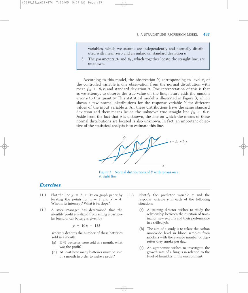
According to this model, the observation Yi corresponding to level xi ofthe controlled variable is one observation from the normal distribution withmean �0 � �1xi and standard deviation �. One interpretation of this is thatas we attempt to observe the true value on the line, nature adds the randomerror e to this quantity. This statistical model is illustrated in Figure 3, whichshows a few normal distributions for the response variable Y for differentvalues of the input variable x. All these distributions have the same standarddeviation and their means lie on the unknown true straight line �0 � �1x.Aside from the fact that � is unknown, the line on which the means of thesenormal distributions are located is also unknown. In fact, an important objec-tive of the statistical analysis is to estimate this line.
3. A STRAIGHT LINE REGRESSION MODEL 437
variables, which we assume are independently and normally distrib-uted with mean zero and an unknown standard deviation �.
3. The parameters �0 and �1 , which together locate the straight line, areunknown.
y
y = x
x
+0β 1β
Figure 3 Normal distributions of Y with means on astraight line.
Exercises
11.1 Plot the line on graph paper bylocating the points for and What is its intercept? What is its slope?
11.2 A store manager has determined that themonthly profit y realized from selling a particu-lar brand of car battery is given by
where x denotes the number of these batteriessold in a month.
(a) If 41 batteries were sold in a month, whatwas the profit?
(b) At least how many batteries must be soldin a month in order to make a profit?
y � 10 x � 155
x � 4.x � 1y � 2 � 3x 11.3 Identify the predictor variable x and the
response variable y in each of the followingsituations.
(a) A training director wishes to study therelationship between the duration of train-ing for new recruits and their performancein a skilled job.
(b) The aim of a study is to relate the carbonmonoxide level in blood samples fromsmokers with the average number of ciga-rettes they smoke per day.
(c) An agronomist wishes to investigate thegrowth rate of a fungus in relation to thelevel of humidity in the environment.
45688_11_p429-474 7/25/05 9:57 AM Page 437
(d) A market analyst wishes to relate theexpenditures incurred in promoting aproduct in test markets and the subsequentamount of product sales.
11.4 Identify the values of the parameters �0 , �1 ,and � in the statistical model
where e is a normal random variable with mean0 and standard deviation 5.
11.5 Identify the values of the parameters �0 , �1 ,and � in the statistical model
where e is a normal random variable with mean 0and standard deviation 3.
11.6 Under the linear regression model:
(a) Determine the mean and standard devia-tion of Y, for x � 4, when �0 � 1,�1 � 3, and � � 2.
(b) Repeat part (a) with x � 2.
11.7 Under the linear regression model:
(a) Determine the mean and standard devia-tion of Y, for x � 1, when �0 � 3,�1 � � 4, and � � 4.
(b) Repeat part (a) with x � 2.
Y � 7 � 5x � e
Y � 2 � 4x � e
438 CHAPTER 11/REGRESSION ANALYSIS I
11.8 Graph the straight line for the means of thelinear regression model
having �0 � �3, �1 � 4, and the normalrandom variable e has standard deviation 3.
11.9 Graph the straight line for the means of thelinear regression model having �0 � 7 and �1 � 2.
11.10 Consider the linear regression model
where �0 � �2, �1 � �1, and the normalrandom variable e has standard deviation 3.
(a) What is the mean of the response Y whenx � 3? When x � 6?
(b) Will the response at x � 3 always belarger than that at x � 6? Explain.
11.11 Consider the following linear regression modelwhere �0 � 4, �1 � 3,
and the normal random variable e has the stan-dard deviation 4.
(a) What is the mean of the response Y whenx � 4? When x � 5?
(b) Will the response at x � 5 always belarger than that at x � 4? Explain.
Y � �0 � �1x � e,
Y � �0 � �1x � e
Y � �0 � �1x � e
Y � �0 � �1x � e
4. THE METHOD OF LEAST SQUARES
Let us tentatively assume that the preceding formulation of the model is cor-rect. We can then proceed to estimate the regression line and solve a fewrelated inference problems. The problem of estimating the regression parame-ters �0 and �1 can be viewed as fitting the best straight line of the y to x rela-tionship in the scatter diagram. One can draw a line by eyeballing the scatterdiagram, but such a judgment may be open to dispute. Moreover, statisticalinferences cannot be based on a line that is estimated subjectively. On theother hand, the method of least squares is an objective and efficient methodof determining the best fitting straight line. Moreover, this method is quiteversatile because its application extends beyond the simple straight lineregression model.
Suppose that an arbitrary line is drawn on the scatter diagramas it is in Figure 4. At the value xi of the independent variable, the y value pre-dicted by this line is whereas the observed value is yi . The discrepancyb0 � b1xi
y � b0 � b1x
45688_11_p429-474 7/25/05 9:58 AM Page 438

between the observed and predicted y values is then which is the vertical distance of the point from the line.
Considering such discrepancies at all the n points, we take
as an overall measure of the discrepancy of the observed points from the trial lineThe magnitude of D obviously depends on the line that is drawn.
In other words, it depends on b0 and b1 , the two quantities that determine the trialline. A good fit will make D as small as possible. We now state the principle of leastsquares in general terms to indicate its usefulness to fitting many other models.
For the straight line model, the least squares principle involves the determi-nation of b0 and b1 to minimize.
D � �n
i � 1 ( yi � b0 � b1xi )
2
y � b0 � b1x.
D � �n
i � 1 di
2 � �n
i � 1 ( yi � b0 � b1xi )
2
yi � b0 � b1xi � di ,
4. THE METHOD OF LEAST SQUARES 439
y = b0 + b1x
b0 + b1xi
di = (yi – b0 – b1xi)
yi
xi x
y
Figure 4 Deviations of the observations from a liney � b0 � b1x.
The Principle of Least Squares
Determine the values for the parameters so that the overall discrepancy
is minimized.The parameter values thus determined are called the least squares
estimates.
D � � (Observed response � Predicted response)2
45688_11_p429-474 7/27/05 3:07 PM Page 439

The quantities b0 and b1 thus determined are denoted by and respec-tively, and called the least squares estimates of the regression parameters�0 and �1 . The best fitting straight line or best fitting regression line is thengiven by the equation
To describe the formulas for the least squares estimators, we first introducesome basic notation.
The quantities and are the sample means of the x and y values; Sxx andSyy are the sums of squared deviations from the means, and Sxy is the sum ofthe cross products of deviations. These five summary statistics are the keyingredients for calculating the least squares estimates and handling the infer-ence problems associated with the linear regression model. The reader mayreview Sections 5 and 6 of Chapter 3 where calculations of these statisticswere illustrated.
The formulas for the least squares estimators are
yx
y � �0 � �1x
�1 ,�0
440 CHAPTER 11/REGRESSION ANALYSIS I
Basic Notation
Sxy � � (x � x)(y � y ) � � xy ��� x��� y�
n
Syy � � ( y � y )2 � � y2 ��� y�2
n
Sxx � � ( x � x)2 � � x2 ��� x�2
n
x �1n
� x y �1n
� y
Least squares estimator of �0
Least squares estimator of �1
� 1 �Sxy
Sxx
� 0 � y � � 1x
45688_11_p429-474 7/25/05 9:58 AM Page 440
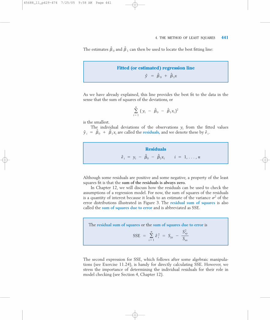
The estimates and can then be used to locate the best fitting line:
As we have already explained, this line provides the best fit to the data in thesense that the sum of squares of the deviations, or
is the smallest.The individual deviations of the observations yi from the fitted values
are called the residuals, and we denote these by
Although some residuals are positive and some negative, a property of the leastsquares fit is that the sum of the residuals is always zero.
In Chapter 12, we will discuss how the residuals can be used to check theassumptions of a regression model. For now, the sum of squares of the residualsis a quantity of interest because it leads to an estimate of the variance �2 of theerror distributions illustrated in Figure 3. The residual sum of squares is alsocalled the sum of squares due to error and is abbreviated as SSE.
The second expression for SSE, which follows after some algebraic manipula-tions (see Exercise 11.24), is handy for directly calculating SSE. However, westress the importance of determining the individual residuals for their role inmodel checking (see Section 4, Chapter 12).
e i .y i � �0 � �1xi
�n
i � 1 ( yi � �0 � �1xi )
2
� 1� 0
4. THE METHOD OF LEAST SQUARES 441
Fitted (or estimated) regression line
y � � 0 � � 1x
Residuals
e i � yi � �0 � �1xi i � 1, . . . , n
The residual sum of squares or the sum of squares due to error is
SSE � �n
i � 1 e i
2 � Syy �Sxy
2
Sxx
45688_11_p429-474 7/25/05 9:58 AM Page 441

An estimate of variance �2 is obtained by dividing SSE by n � 2. Thereduction by 2 is because two degrees of freedom are lost from estimating thetwo parameters �0 and �1 .
In applying the least squares method to a given data set, we first computethe basic quantities Sxx, Syy, and Sxy. Then the preceding formulas can beused to obtain the least squares regression line, the residuals, and the value ofSSE. Computations for the data given in Table 1 are illustrated in Table 3.
x , y ,
442 CHAPTER 11/REGRESSION ANALYSIS I
TABLE 3 Computations for the Least Squares Line, SSE, and Residuals Using the Data of Table 1
x y x2 y2 xy Residual
3 9 9 81 27 7.15 1.853 5 9 25 15 7.15 �2.154 12 16 144 48 9.89 2.115 9 25 81 45 12.63 �3.636 14 36 196 84 15.37 �1.376 16 36 256 96 15.37 .637 22 49 484 154 18.11 3.898 18 64 324 144 20.85 �2.858 24 64 576 192 20.85 3.159 22 81 484 198 23.59 �1.59
Total 59 151 389 2651 1003 .04 (rounding error)
Sxy � 1003 �59 � 151
10� 112.1
SSE � 370.9 �(112.1)2
40.9� 63.6528Syy � 2651 �
(151)2
10� 370.9
�0 � 15.1 � 2.74 � 5.9 � �1.07Sxx � 389 �(59)2
10� 40.9
�1 �112.140.9
� 2.74y � 15.1x � 5.9,
e� 0 � � 1x
Estimate of Variance
The estimator of the error variance �2 is
S2 �SSE
n � 2
45688_11_p429-474 7/25/05 9:58 AM Page 442

4. THE METHOD OF LEAST SQUARES 443
y = –1.07 + 2.74x
y
25
20
15
10
5
0 2 4 6 8 10 x
Figure 5 The least squares regression line for thedata given in Table 1.
The equation of the line fitted by the least squares method is then
Figure 5 shows a plot of the data along with the fitted regression line.The residuals are computed in the
last column of Table 3. The sum of squares of the residuals is
which agrees with our previous calculations of SSE, except for the error due torounding. Theoretically, the sum of the residuals should be zero, and the differ-ence between the sum .04 and zero is also due to rounding.
The estimate of the variance �2 is
The calculations involved in a regression analysis become increasinglytedious with larger data sets. Access to a computer proves to be a considerableadvantage. Table 4 illustrates a part of the computer-based analysis of linearregression using the data of Example 4 and the MINITAB package. For a morecomplete regression analysis, see Table 5 in Section 6.4.
s2 �SSE
n � 2�
63.65288
� 7.96
�n
i � 1 e i
2 � (1.85)2 � (�2.15)2 � (2.11)2 � � � � � (�1.59)2 � 63.653
e i � yi � y i � yi � 1.07 � 2.74xi
y � �1.07 � 2.74 x
45688_11_p429-474 7/25/05 9:58 AM Page 443

Exercises
444 CHAPTER 11/REGRESSION ANALYSIS I
Data: C11T3 DAT
C1: 3 3 4 5 6 6 7 8 8 9
C2: 9 5 12 9 14 16 22 18 24 22
Dialog box:
Stat Regression Regression
Type C2 in Response
Type C1 in Predictors. Click OK.
Output:
Regression Analysis
The regression equation is
y � �1.07 � 2.74x
TABLE 4 Regression Analysis of the Data in Table 1, Example 4, Using MINITAB
11.12 Given the five pairs of (x, y) values
x 0 1 6 3 5
y 6 5 2 4 3
(a) Construct a scatter diagram.
(b) Calculate and Syy .
(c) Calculate the least squares estimatesand
(d) Determine the fitted line and draw theline on the scatter diagram.
11.13 Given these six pairs of (x, y) values,
x 1 2 3 3 4 5
y 8 4 5 2 2 0
(a) Plot the scatter diagram.
(b) Calculate and Syy .
(c) Calculate the least squares estimates and
(d) Determine the fitted line and draw theline on the scatter diagram.
� 1 .� 0
x , y, Sxx , Sxy ,
� 1 .� 0
x , y, Sxx , Sxy ,
11.14 Refer to Exercise 11.12.
(a) Find the residuals and verify that theysum to zero.
(b) Calculate the residual sum of squaresSSE by
(i) Adding the squares of the residuals.
(ii) Using the formula SSE �
(c) Obtain the estimate of �2.
11.15 Refer to Exercise 11.13.
(a) Find the residuals and verify that theysum to zero.
(b) Calculate the residual sums of squaresSSE by
(i) Adding the squares of the residuals.
(ii) Using the formula SSE �
(c) Obtain the estimate of �2.
Sxy2 / SxxSyy �
Sxy2 / SxxSyy �
45688_11_p429-474 7/27/05 3:07 PM Page 444

11.16 Given the five pairs of (x, y) values
x 0 1 2 3 4
y 3 2 5 6 9
(a) Calculate and Syy.
(b) Calculate the least squares estimates and
(c) Determine the fitted line.
11.17 Given the five pairs of (x, y) values
x 0 2 4 6 8
y 4 3 6 8 9
(a) Calculate and Syy.
(b) Calculate the least squares estimates and
(c) Determine the fitted line.
11.18 Computing from a data set of (x, y)values, we obtained the following summarystatistics.
(a) Obtain the equation of the best fittingstraight line.
(b) Calculate the residual sum of squares.
(c) Estimate �2.
11.19 Computing from a data set of (x, y)values, we obtained the following summarystatistics.
(a) Obtain the equation of the best fittingstraight line.
(b) Calculate the residual sum of squares.
(c) Estimate �2.
Sxx � 28.2 Sxy � 3.25 Syy � 2.01 n � 20 x � 1.4 y � 5.2
Sxx � 10.82 Sxy � 2.677 Syy � 1.125 n � 14 x � 3.5 y � 2.84
�1 .�0
x , y, Sxx , Sxy ,
�1 .�0
x , y, Sxx , Sxy ,
4. THE METHOD OF LEAST SQUARES 445
11.20 The data on female wolves in Table D.9 of theData Bank concerning body weight (lb) andbody length (cm) are
Weight 57 84 90 71 77 68 73
Body length 123 129 143 125 122 125 122
(a) Obtain the least squares fit of bodyweight to the predictor body length.
(b) Calculate the residual sum of squares.
(c) Estimate � 2.
11.21 Refer to the data on female wolves in Exercise11.20.
(a) Obtain the least squares fit of body lengthto the predictor body weight.
(b) Calculate the residual sum of squares.
(c) Estimate �2.
(d) Compare your answer in part (a) withyour answer to part (a) of Exercise 11.20.Should the two answers be the same?Why or why not?
11.22 Using the formulas of and SSE, show thatSSE can also be expressed as
(a)
(b)
11.23 Referring to the formulas of and showthat the point lies on the fitted regres-sion line.
11.24 To see why the residuals always sum to zero,refer to the formulas of and and verifythat
(a) The predicted values are
(b) The residuals are
Then show that
(c) Verify that
2�1Sxy � Syy � Sxy2 / Sxx .
�n
i � 1 e i
2 � Syy � � 12Sxx �
�n
i � 1 e i � 0.
(yi � y ) � �1(xi � x )e i � yi � y i �
�1(xi � x ) .y i � y �
�1 �0
( x , y )�1 ,�0
SSE � Syy � �12 Sxx
SSE � Syy � �1Sxy
�1
45688_11_p429-474 7/27/05 3:08 PM Page 445

5. THE SAMPLING VARIABILITY OF THE LEAST SQUARES ESTIMATORS—TOOLS FOR INFERENCE
It is important to remember that the line obtained by theprinciple of least squares is an estimate of the unknown true regression line y �
In our drug evaluation problem (Example 4), the estimated line is
Its slope suggests that the mean duration of relief increases by 2.74days for each unit dosage of the drug. Also, if we were to estimate the expectedduration of relief for a specified dosage milligrams, we would naturallyuse the fitted regression line to calculate the estimate 11.26 days. A few questions concerning these estimates naturally arise at this point.
1. In light of the value 2.74 for could the slope �1 of the true regres-sion line be as much as 4? Could it be zero so that the true regressionline is which does not depend on x? What are the plausiblevalues for �1 ?
2. How much uncertainty should be attached to the estimated duration of11.26 days corresponding to the given dosage
To answer these and related questions, we must know something about thesampling distributions of the least squares estimators. These sampling distributionswill enable us to test hypotheses and set confidence intervals for the parameters�0 and �1 that determine the straight line and for the straight line itself. Again, thet distribution is relevant.
x* � 4.5?
y � �0 ,
�1 ,
�1.07 � 2.74 � 4.5 �x* � 4.5
�1 � 2.74
y � �1.07 � 2.74 x
�0 � �1x.
y � �0 � �1x
446 CHAPTER 11/REGRESSION ANALYSIS I
1. The standard deviations (also called standard errors) of the leastsquares estimators are
To estimate the standard error, use
S � � SSEn � 2
in place of �
S.E.( �1) ��
√Sxx
S.E.( � 0) � � � 1n
�x2
Sxx
2. Inferences about the slope �1 are based on the t distribution
T ��1 � �1
S / √Sxx
d.f. � n � 2
45688_11_p429-474 7/25/05 9:58 AM Page 446

6. IMPORTANT INFERENCE PROBLEMS 447
Inferences about the intercept �0 are based on the t distribution
T ��0 � �0
S � 1n
�x2
Sxx
d.f. � n � 2
3. At a specified value the expected response is �0 � �1x*. Thisis estimated by with
Estimated standard error
Inferences about �0 � �1x* are based on the t distribution
T �(�0 � �1x*) � (�0 � �1x*)
S � 1n
�(x* � x )2
Sxx
d.f. � n � 2
S � 1n
�(x* � x )2
Sxx
�0 � �1x*x � x*,
6. IMPORTANT INFERENCE PROBLEMS
We are now prepared to test hypotheses, construct confidence intervals, andmake predictions in the context of straight line regression.
6.1. INFERENCE CONCERNING THE SLOPE �1
In a regression analysis problem, it is of special interest to determine whetherthe expected response does or does not vary with the magnitude of the inputvariable x. According to the linear regression model,
Expected response � �0 � �1x
This does not change with a change in x if and only if �1 � 0. We can thereforetest the null hypothesis H0��1 � 0 against a one- or a two-sided alternative,depending on the nature of the relation that is anticipated. If we refer to theboxed statement (2) of Section 5, the null hypothesis H0��1 � 0 is to betested using the test statistic
T ��1
S / √Sxx
d.f. � n � 2
45688_11_p429-474 7/27/05 3:08 PM Page 447

Example 5 A Test to Establish That Duration of Relief Increases with DosageDo the data given in Table 1 constitute strong evidence that the mean dura-tion of relief increases with higher dosages of the drug?
SOLUTION For an increasing relation, we must have �1 � 0. Therefore, we are to test the null hypothesis H0��1 � 0 versus the one-sided alternative H1��1 �0. We select � .05. Since t.05 � 1.860, with d.f. � 8 we set the rejec-tion region R�T 1.860. Using the calculations that follow Table 2, wehave
The observed t value is in the rejection region, so H0 is rejected. Moreover,6.213 is much larger than t.005 � 3.355, so the P–value is much smallerthan .005.
A computer calculation gives There is strongevidence that larger dosages of the drug tend to increase the duration of reliefover the range covered in the study.
A warning is in order here concerning the interpretation of the test ofH0 :�1 � 0. If H0 is not rejected, we may be tempted to conclude that y doesnot depend on x. Such an unqualified statement may be erroneous. First,the absence of a linear relation has only been established over the range ofthe x values in the experiment. It may be that x was just not varied enough toinfluence y. Second, the interpretation of lack of dependence on x is validonly if our model formulation is correct. If the scatter diagram depicts arelation on a curve but we inadvertently formulate a linear model and testH0��1 � 0, the conclusion that H0 is not rejected should be interpreted tomean “no linear relation,” rather than “no relation.” We elaborate on this pointfurther in Section 7. Our present viewpoint is to assume that the model iscorrectly formulated and discuss the various inference problems associatedwith it.
More generally, we may test whether or not �1 is equal to some specifiedvalue �10 , not necessarily zero.
P[T � 6.213] � .0001.
Test statistic t �2.74.441
� 6.213
Estimated S.E.( �1) �s
√Sxx
�2.8207
√40.90� .441
s2 �SSE
n � 2�
63.65288
� 7.9566, s � 2.8207
�1 � 2.74
448 CHAPTER 11/REGRESSION ANALYSIS I
45688_11_p429-474 7/25/05 9:58 AM Page 448
In addition to testing hypotheses, we can provide a confidence interval forthe parameter �1 using the t distribution.
Example 6 A Confidence Interval for �1
Construct a 95% confidence interval for the slope of the regression line inreference to the data of Table 1.
SOLUTION In Example 5, we found that and The requiredconfidence interval is given by
We are 95% confident that by adding one extra milligram to the dosage, themean duration of relief would increase somewhere between 1.72 and 3.76 days.
6.2. INFERENCE ABOUT THE INTERCEPT �0
Although somewhat less important in practice, inferences similar to those out-lined in Section 6.1 can be provided for the parameter �0 . The procedures areagain based on the t distribution with d.f. � n � 2, stated for in Section 5.In particular,
�0
2.74 � 2.306 � .441 � 2.74 � 1.02 or (1.72, 3.76)
s / √Sxx � .441.�1 � 2.74
6. IMPORTANT INFERENCE PROBLEMS 449
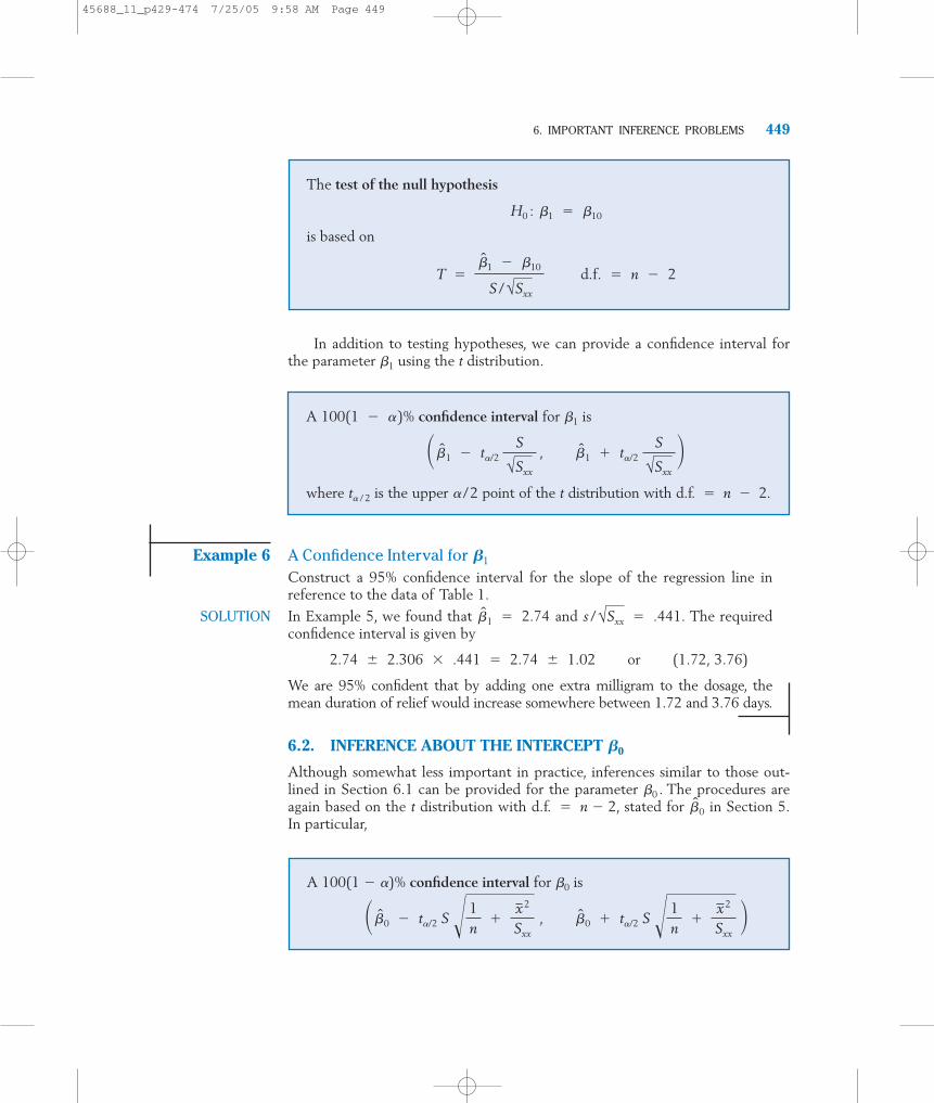
The test of the null hypothesis
is based on
T ��1 � �10
S / √Sxx
d.f. � n � 2
H0 : �1 � �10
A 100(1 � )% confidence interval for �1 is
where t / 2 is the upper /2 point of the t distribution with d.f. � n � 2.
� �1 � t/2 S
√Sxx
, �1 � t/2 S
√Sxx�
A 100(1 � )% confidence interval for �0 is
� �0 � t/2 S � 1n
�x2
Sxx , �0 � t/2 S � 1
n�
x2
Sxx�
45688_11_p429-474 7/25/05 9:58 AM Page 449
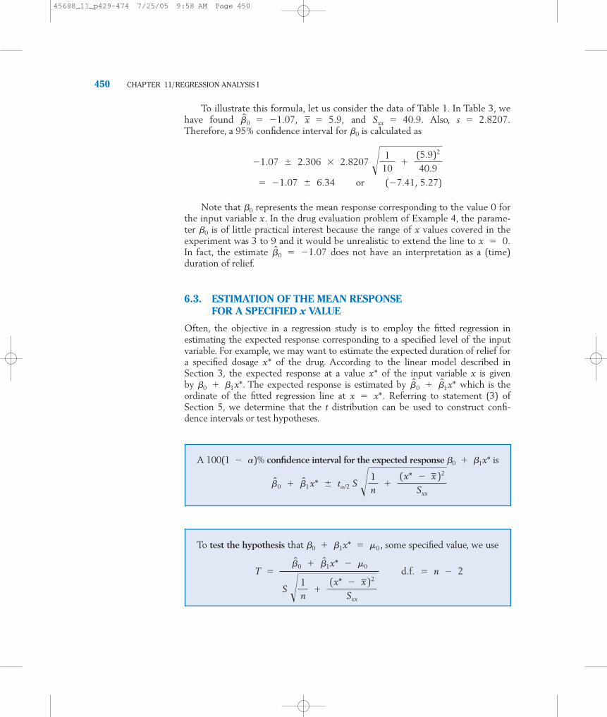
To illustrate this formula, let us consider the data of Table 1. In Table 3, wehave found and Also,Therefore, a 95% confidence interval for �0 is calculated as
Note that �0 represents the mean response corresponding to the value 0 forthe input variable x. In the drug evaluation problem of Example 4, the parame-ter �0 is of little practical interest because the range of x values covered in theexperiment was 3 to 9 and it would be unrealistic to extend the line to In fact, the estimate does not have an interpretation as a (time)duration of relief.
6.3. ESTIMATION OF THE MEAN RESPONSE FOR A SPECIFIED x VALUE
Often, the objective in a regression study is to employ the fitted regression inestimating the expected response corresponding to a specified level of the inputvariable. For example, we may want to estimate the expected duration of relief fora specified dosage x* of the drug. According to the linear model described inSection 3, the expected response at a value x* of the input variable x is givenby �0 � �1x*. The expected response is estimated by � which is theordinate of the fitted regression line at Referring to statement (3) ofSection 5, we determine that the t distribution can be used to construct confi-dence intervals or test hypotheses.
x � x*.�1x*�0
�0 � �1.07x � 0.
� �1.07 � 6.34 or (�7.41, 5.27)
�1.07 � 2.306 � 2.8207 � 110
�(5.9)2
40.9
s � 2.8207.Sxx � 40.9.x � 5.9,�0 � �1.07,
450 CHAPTER 11/REGRESSION ANALYSIS I
A 100(1 � )% confidence interval for the expected response �0 � �1x* is
�0 � �1x* � t/2 S � 1n
�(x* � x )2
Sxx
To test the hypothesis that �0 � �1x* � �0 , some specified value, we use
T ��0 � �1x* � �0
S � 1n
�(x* � x )2
Sxx
d.f. � n � 2
45688_11_p429-474 7/25/05 9:58 AM Page 450

Example 7 A Confidence Interval for the Expected Duration of ReliefAgain consider the data given in Table 1 and the calculations for the regressionanalysis given in Table 3. Obtain a 95% confidence interval for the expectedduration of relief when the dosage is (a) and (b)
SOLUTION The fitted regression line is
The expected duration of relief corresponding to the dosage mil-ligrams of the drug is estimated as
A 95% confidence interval for the mean duration of relief with the dosageis therefore
We are 95% confident that 6 milligrams of the drug produces an averageduration of relief that is between about 13.3 and 17.4 days.
Suppose that we also wish to estimate the mean duration of relief underthe dosage We follow the same steps to calculate the pointestimate.
A 95% confidence interval is
The formula for the standard error shows that when x* is close to thestandard error is smaller than it is when x* is far removed from This isconfirmed by Example 7, where the standard error at x* � 9.5 can be seento be more than twice as large as the value at x* � 6. Consequently, theconfidence interval for the former is also wider. In general, estimation is moreprecise near the mean than it is for values of the x variable that lie far fromthe mean.
x
x.x,
24.96 � 2.306 � 1.821 � 24.96 � 4.20 or (20.76, 29.16)
� 1.821
Estimated standard error � 2.8207 � 110
�(9.5 � 5.9)2
40.9
�0 � �1x* � �1.07 � 2.74 � 9.5 � 24.96 days
x* � 9.5.
� 15.37 � 2.06 or (13.31, 17.43)15.37 � t.025 � .893 � 15.37 � 2.306 � .893
x* � 6
� 2.8207 � .3166 � .893
Estimated standard error � s � 110
�(6 � 5.9)2
40.9
�0 � �1x* � �1.07 � 2.74 � 6 � 15.37 days
x* � 6
y � �1.07 � 2.74x
x* � 9.5.x* � 6
6. IMPORTANT INFERENCE PROBLEMS 451
45688_11_p429-474 7/25/05 9:58 AM Page 451

Caution: Extreme caution should be exercised in extending a fittedregression line to make long-range predictions far away from the range ofx values covered in the experiment. Not only does the confidence intervalbecome so wide that predictions based on it can be extremely unreliable, butan even greater danger exists. If the pattern of the relationship between thevariables changes drastically at a distant value of x, the data provide no infor-mation with which to detect such a change. Figure 6 illustrates this situation.We would observe a good linear relationship if we experimented with x valuesin the 5 to 10 range, but if the fitted line were extended to estimate theresponse at x* � 20, then our estimate would drastically miss the mark.
452 CHAPTER 11/REGRESSION ANALYSIS I
Predicted
True relation
y
5 10 20 x
Figure 6 Danger in long-range prediction.
The estimated standard error when predicting a single observation y at agiven x* is
S �1 �1n
�(x* � x)2
Sxx
6.4. PREDICTION OF A SINGLE RESPONSE FOR A SPECIFIED x VALUE
Suppose that we give a specified dosage x* of the drug to a single patient and wewant to predict the duration of relief from the symptoms of allergy. This problemis different from the one considered in Section 6.3, where we were interested inestimating the mean duration of relief for the population of all patients given thedosage x*. The prediction is still determined from the fitted line; that is, the pre-dicted value of the response is as it was in the preceding case. How-ever, the standard error of the prediction here is larger, because a single observationis more uncertain than the mean of the population distribution. We now give theformula of the estimated standard error for this case.
�0 � �1x*
45688_11_p429-474 7/25/05 9:58 AM Page 452
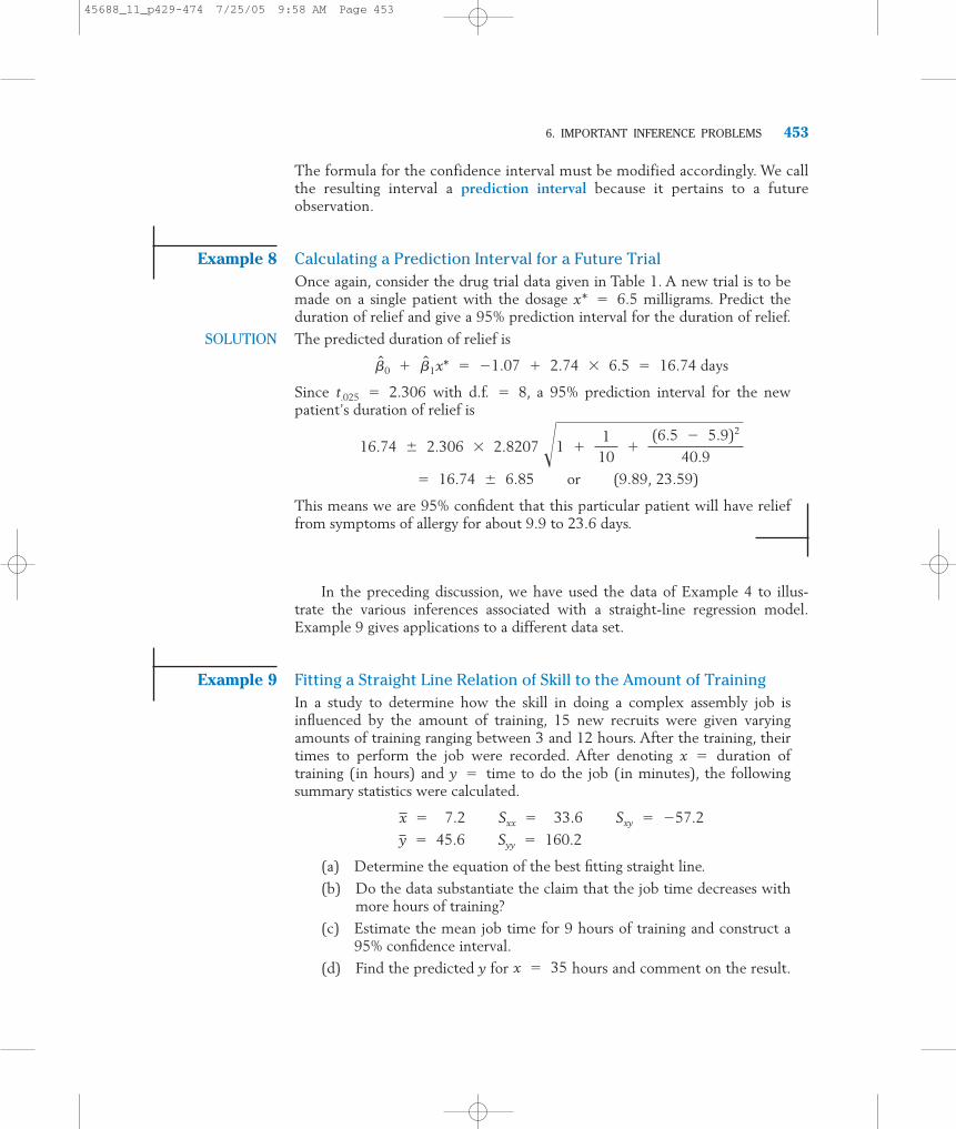
The formula for the confidence interval must be modified accordingly. We callthe resulting interval a prediction interval because it pertains to a futureobservation.
Example 8 Calculating a Prediction Interval for a Future TrialOnce again, consider the drug trial data given in Table 1. A new trial is to bemade on a single patient with the dosage x* � 6.5 milligrams. Predict theduration of relief and give a 95% prediction interval for the duration of relief.
SOLUTION The predicted duration of relief is
Since with d.f. � 8, a 95% prediction interval for the newpatient’s duration of relief is
This means we are 95% confident that this particular patient will have relieffrom symptoms of allergy for about 9.9 to 23.6 days.
In the preceding discussion, we have used the data of Example 4 to illus-trate the various inferences associated with a straight-line regression model.Example 9 gives applications to a different data set.
Example 9 Fitting a Straight Line Relation of Skill to the Amount of TrainingIn a study to determine how the skill in doing a complex assembly job isinfluenced by the amount of training, 15 new recruits were given varyingamounts of training ranging between 3 and 12 hours. After the training, theirtimes to perform the job were recorded. After denoting x � duration oftraining (in hours) and y � time to do the job (in minutes), the followingsummary statistics were calculated.
(a) Determine the equation of the best fitting straight line.
(b) Do the data substantiate the claim that the job time decreases withmore hours of training?
(c) Estimate the mean job time for 9 hours of training and construct a95% confidence interval.
(d) Find the predicted y for hours and comment on the result.x � 35
y � 45.6 Syy � 160.2
x � 7.2 Sxx � 33.6 Sxy � �57.2
� 16.74 � 6.85 or (9.89, 23.59)
16.74 � 2.306 � 2.8207 �1 �110
�(6.5 � 5.9)2
40.9
t.025 � 2.306
�0 � �1x* � �1.07 � 2.74 � 6.5 � 16.74 days
6. IMPORTANT INFERENCE PROBLEMS 453
45688_11_p429-474 7/25/05 9:58 AM Page 453
SOLUTION Using the summary statistics we find:
(a) The least squares estimates are
So, the equation of the fitted line is
(b) To answer this question, we are to test H0��1 � 0 versus H1��1 0.The test statistic is
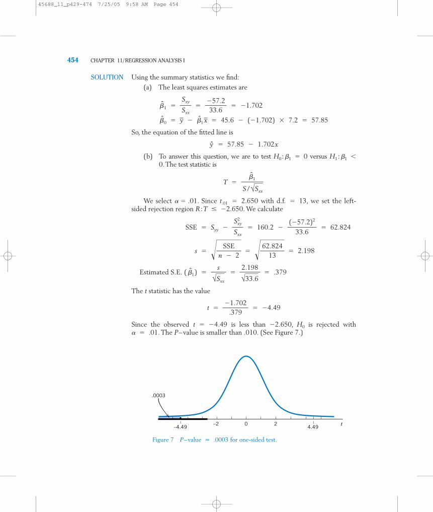
We select � .01. Since with d.f. � 13, we set the left-sided rejection region R�T � �2.650. We calculate
The t statistic has the value
Since the observed is less than �2.650, H0 is rejected with � .01. The P–value is smaller than .010. (See Figure 7.)
t � �4.49
t ��1.702
.379� �4.49
Estimated S.E. ( �1) �s
√Sxx
�2.198
√33.6� .379
s � � SSEn � 2
� � 62.82413
� 2.198
SSE � Syy �Sxy
2
Sxx� 160.2 �
(�57.2)2
33.6� 62.824
t.01 � 2.650
T ��1
S / √Sxx
y � 57.85 � 1.702x
�0 � y � �1x � 45.6 � (�1.702) � 7.2 � 57.85
�1 �Sxy
Sxx�
�57.233.6
� �1.702
454 CHAPTER 11/REGRESSION ANALYSIS I
.0003
0–2 2 t–4.49 4.49
Figure 7 P–value � .0003 for one-sided test.
45688_11_p429-474 7/25/05 9:58 AM Page 454
A computer calculation gives
We conclude that increasing the duration of training significantly reduces themean job time within the range covered in the experiment.
(c) The expected job time corresponding to x* � 9 hours is estimated as
and its
Since with d.f. � 13, the required confidence interval is
(d) Since hours is far beyond the experimental range of 3 to12 hours, it is not sensible to predict y at using the fittedregression line. Here a formal calculation gives
which is a nonsensical result.
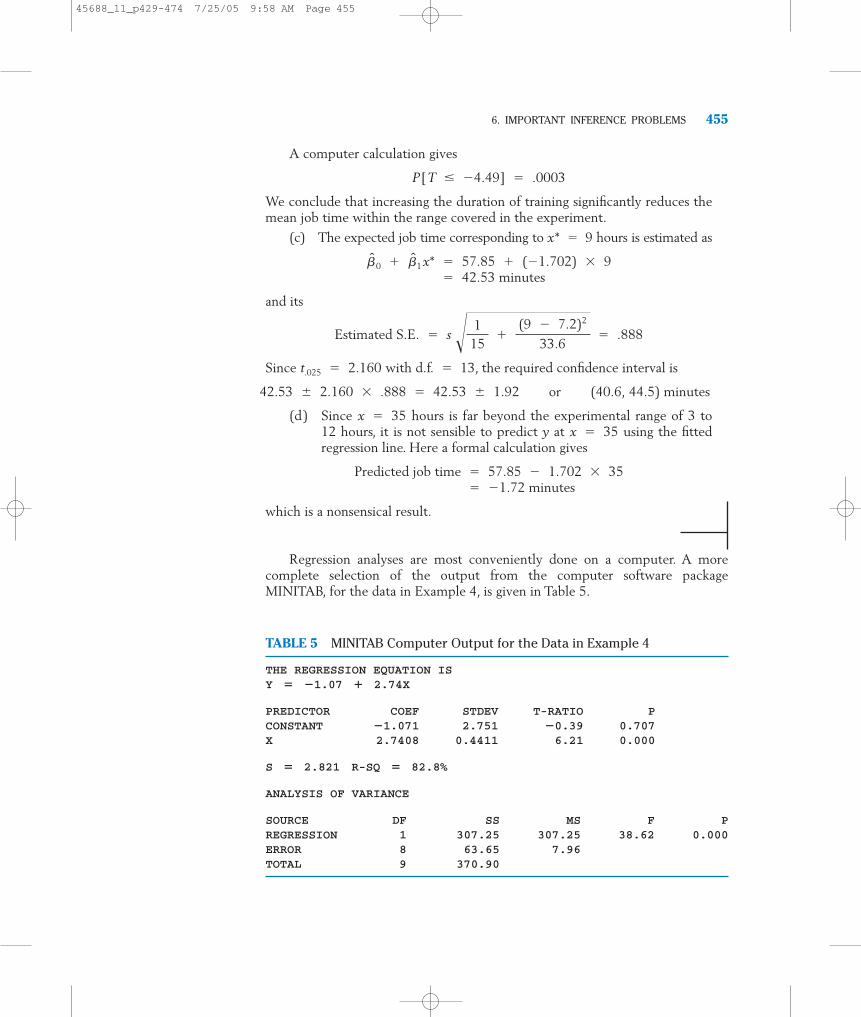
Regression analyses are most conveniently done on a computer. A morecomplete selection of the output from the computer software packageMINITAB, for the data in Example 4, is given in Table 5.
� �1.72 minutes Predicted job time � 57.85 � 1.702 � 35
x � 35x � 35
42.53 � 2.160 � .888 � 42.53 � 1.92 or (40.6, 44.5) minutes
t.025 � 2.160
Estimated S.E. � s � 115
�(9 � 7.2)2
33.6� .888
� 42.53 minutes �0 � �1x* � 57.85 � (�1.702) � 9
P[T � �4.49] � .0003
6. IMPORTANT INFERENCE PROBLEMS 455
TABLE 5 MINITAB Computer Output for the Data in Example 4
THE REGRESSION EQUATION ISY � �1.07 � 2.74X
PREDICTOR COEF STDEV T-RATIO PCONSTANT �1.071 2.751 �0.39 0.707X 2.7408 0.4411 6.21 0.000
S � 2.821 R-SQ � 82.8%
ANALYSIS OF VARIANCE
SOURCE DF SS MS F PREGRESSION 1 307.25 307.25 38.62 0.000ERROR 8 63.65 7.96TOTAL 9 370.90
45688_11_p429-474 7/25/05 9:58 AM Page 455

The output of the computer software package SAS for the data in Example 4is given in Table 6. Notice the similarity of information in Tables 5 and 6. Bothinclude the least squares estimates of the coefficients, their estimated standarddeviations, and the t test for testing that the coefficient is zero. The estimate of �2 ispresented as the mean square error in the analysis of variance table.
456 CHAPTER 11/REGRESSION ANALYSIS I
TABLE 6 SAS Computer Output for the Data in Example 4
MODEL: MODEL 1DEPENDENT VARIABLE: Y
ANALYSIS OF VARIANCE
SUM OF MEANSOURCE DF SQUARES SQUARE F VALUE PROB � F
MODEL 1 307.24719 307.24719 38.615 0.0003ERROR 8 63.65281 7.95660C TOTAL 9 370.90000
ROOT MSE 2.82074 R-SQUARE 0.8284
PARAMETER ESTIMATES
PARAMETER STANDARD T FOR HO:VARIABLE DF ESTIMATE ERROR PARAMETER � 0 PROB
INTERCEP 1 �1.070905 2.75091359 �0.389 0.7072X1 1 2.740831 0.44106455 6.214 0.0003
� � T �
Example 10 Predicting the Number of Situps after a Semester of ConditioningRefer to the physical fitness data in Table D.5 of the Data Bank. Using thedata on numbers of situps:
(a) Find the least squares fitted line to predict the posttest number ofsitups from the pretest number at the start of the conditioning class.
(b) Find a 95% confidence interval for the mean number of posttest situpsfor persons who can perform 35 situps in the pretest. Also find a 95%prediction interval for the number of posttest situps that will be per-formed by a new person this semester who does 35 situps in thepretest.
(c) Repeat part (b), but replace the number of pretest situps with 20.
SOLUTION The scatter plot in Figure 8 suggests that a straight line may model theexpected value of posttest situps given the number of pretest situps. Here x isthe number of pretest situps and y is the number of posttest situps. We useMINITAB statistical software to obtain the output
45688_11_p429-474 7/25/05 9:58 AM Page 456

Regression Analysis: Post Situps versus Pre Situps
The regression equation isPost Situps = 10.3 � 0.899 Pre Situps
Predictor Coef SE Coef T PConstant 10.331 2.533 4.08 0.000Pre Situps 0.89904 0.06388 14.07 0.000
S � 5.17893 R-Sq � 71.5% R-Sq(adj) � 71.1%
Analysis of Variance
Source DF SS MS F PRegression 1 5312.9 5312.9 198.09 0.000Residual Error 79 2118.9 26.8Total 80 7431.8
Predicted Values for New Observations
NewObs Pre Sit Fit SE Fit 95% CI 95% PI1 35.0 41.797 0.620 (40.563, 43.032) (31.415, 52.179)2 20.0 28.312 1.321 (25.682, 30.941) (17.673, 38.950)
From the output and s2 �
(5.1789)2 � 26.8 is the estimate of �2.y � �0 � �1x � 10.3 � 0.899x
6. IMPORTANT INFERENCE PROBLEMS 457
70
60
50
40
30
20
20 30 40 50 60
Pos
ttes
t S
itup
s
Pretest Situps
Figure 8 Scatter plot of number of situps.
45688_11_p429-474 7/25/05 9:58 AM Page 457
We have selected the option in MINITAB to obtain the two confi-dence intervals and prediction intervals given in the output. The predic-tion intervals pertain to the posttest number of situps performed by aspecific new person who performed 35 situps in the pretest. The predic-tion intervals are wider than the corresponding confidence intervals forthe expected number of posttest situps for the population of all studentswho would do 35 situps in the pretest. The same relation holds, as itmust, for 20 pretest situps.
Exercises
458 CHAPTER 11/REGRESSION ANALYSIS I
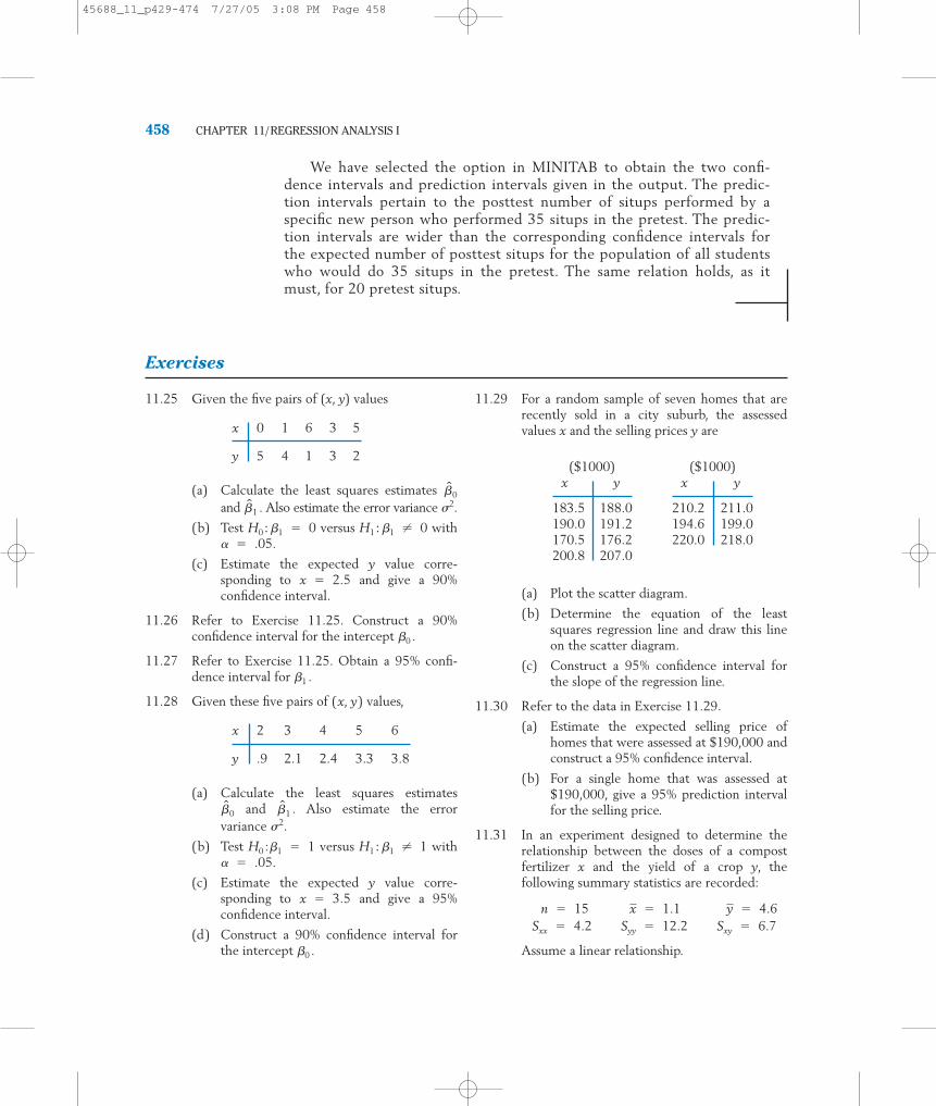
11.25 Given the five pairs of (x, y) values
x 0 1 6 3 5
y 5 4 1 3 2
(a) Calculate the least squares estimates and Also estimate the error variance �2.
(b) Test H0��1 � 0 versus H1��1 � 0 with� � .05.
(c) Estimate the expected y value corre-sponding to and give a 90%confidence interval.
11.26 Refer to Exercise 11.25. Construct a 90%confidence interval for the intercept �0 .
11.27 Refer to Exercise 11.25. Obtain a 95% confi-dence interval for �1 .
11.28 Given these five pairs of (x, y) values,
x 2 3 4 5 6
y .9 2.1 2.4 3.3 3.8
(a) Calculate the least squares estimates and Also estimate the error
variance �2.
(b) Test H0 :�1 � 1 versus H1��1 � 1 with� � .05.
(c) Estimate the expected y value corre-sponding to and give a 95%confidence interval.
(d) Construct a 90% confidence interval forthe intercept �0 .
x � 3.5
�1 .�0
x � 2.5
�1 .�0
11.29 For a random sample of seven homes that arerecently sold in a city suburb, the assessedvalues x and the selling prices y are
(a) Plot the scatter diagram.
(b) Determine the equation of the leastsquares regression line and draw this lineon the scatter diagram.
(c) Construct a 95% confidence interval forthe slope of the regression line.
11.30 Refer to the data in Exercise 11.29.
(a) Estimate the expected selling price ofhomes that were assessed at $190,000 andconstruct a 95% confidence interval.
(b) For a single home that was assessed at$190,000, give a 95% prediction intervalfor the selling price.
11.31 In an experiment designed to determine therelationship between the doses of a compostfertilizer x and the yield of a crop y, thefollowing summary statistics are recorded:
Assume a linear relationship.
Sxx � 4.2 Syy � 12.2 Sxy � 6.7 n � 15 x � 1.1 y � 4.6
($1000)x y
183.5 188.0190.0 191.2170.5 176.2200.8 207.0
($1000)x y
210.2 211.0194.6 199.0220.0 218.0
45688_11_p429-474 7/27/05 3:08 PM Page 458
(a) Find the equation of the least squaresregression line.
(b) Compute the error sum of squares andestimate �2.
(c) Do the data establish the experimenter’sconjecture that, over the range of x valuescovered in the study, the average increasein yield per unit increase in the compostdose is more than 1.3?
11.32 Refer to Exercise 11.31.
(a) Construct a 95% confidence interval forthe expected yield corresponding to
(b) Construct a 95% confidence interval forthe expected yield corresponding to
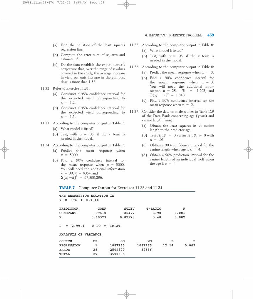
11.33 According to the computer output in Table 7:
(a) What model is fitted?
(b) Test, with � .05, if the x term isneeded in the model.
11.34 According to the computer output in Table 7:
(a) Predict the mean response when
(b) Find a 90% confidence interval forthe mean response when You will need the additional informationn � 30, x � 8354, and
(xi �x)2 � 97,599,296.�
x � 5000.
x � 5000.
x � 1.5.
x � 1.2.
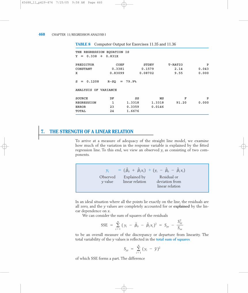
11.35 According to the computer output in Table 8:
(a) What model is fitted?
(b) Test, with � .05, if the x term isneeded in the model.
11.36 According to the computer output in Table 8:
(a) Predict the mean response when
(b) Find a 90% confidence interval forthe mean response when You will need the additional infor-mation n � 25, x � 1.793, and
(c) Find a 90% confidence interval for themean response when
11.37 Consider the data on male wolves in Table D.9of the Data Bank concerning age (years) andcanine length (mm).
(a) Obtain the least squares fit of caninelength to the predictor age.
(b) Test H0��1 � 0 versus H1��1 � 0 with � .05.
(c) Obtain a 90% confidence interval for thecanine length when age is x � 4.
(d) Obtain a 90% prediction interval for thecanine length of an individual wolf whenthe age is x � 4.
x � 2.
(xi � x)2 � 1.848.�
x � 3.
x � 3.
6. IMPORTANT INFERENCE PROBLEMS 459
TABLE 7 Computer Output for Exercises 11.33 and 11.34
THE REGRESSION EQUATION ISY � 994 � 0.104X
PREDICTOR COEF STDEV T-RATIO PCONSTANT 994.0 254.7 3.90 0.001X 0.10373 0.02978 3.48 0.002
S � 2.99.4 R-SQ � 30.2%
ANALYSIS OF VARIANCE
SOURCE DF SS MS F PREGRESSION 1 1087765 1087765 12.14 0.002ERROR 28 2509820 89636TOTAL 29 3597585
45688_11_p429-474 7/25/05 9:58 AM Page 459
460 CHAPTER 11/REGRESSION ANALYSIS I
7. THE STRENGTH OF A LINEAR RELATION
To arrive at a measure of adequacy of the straight line model, we examinehow much of the variation in the response variable is explained by the fittedregression line. To this end, we view an observed yi as consisting of two com-ponents.
In an ideal situation where all the points lie exactly on the line, the residuals areall zero, and the y values are completely accounted for or explained by the lin-ear dependence on x.
We can consider the sum of squares of the residuals
to be an overall measure of the discrepancy or departure from linearity. Thetotal variability of the y values is reflected in the total sum of squares
of which SSE forms a part. The difference
Syy � �n
i � 1 ( yi � y )2
SSE � �n
i � 1 ( yi � �0 � �1xi )
2 � Syy �Sxy
2
Sxx
TABLE 8 Computer Output for Exercises 11.35 and 11.36
THE REGRESSION EQUATION ISY � 0.338 � 0.831X
PREDICTOR COEF STDEV T-RATIO PCONSTANT 0.3381 0.1579 2.14 0.043X 0.83099 0.08702 9.55 0.000
S � 0.1208 R-SQ � 79.9%
ANALYSIS OF VARIANCE
SOURCE DF SS MS F PREGRESSION 1 1.3318 1.3318 91.20 0.000ERROR 23 0.3359 0.0146TOTAL 24 1.6676
yi � �
Observed Explained by Residual ory value linear relation deviation from
linear relation
(yi � �0 � �1xi)( �0 � �1xi)
45688_11_p429-474 7/25/05 9:58 AM Page 460
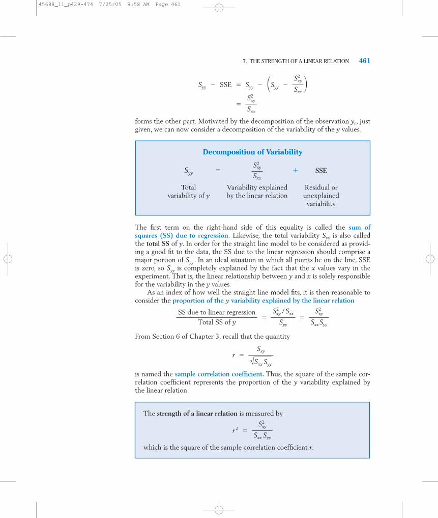
forms the other part. Motivated by the decomposition of the observation yi , justgiven, we can now consider a decomposition of the variability of the y values.
The first term on the right-hand side of this equality is called the sum ofsquares (SS) due to regression. Likewise, the total variability Syy is also calledthe total SS of y. In order for the straight line model to be considered as provid-ing a good fit to the data, the SS due to the linear regression should comprise amajor portion of Syy . In an ideal situation in which all points lie on the line, SSEis zero, so Syy is completely explained by the fact that the x values vary in theexperiment. That is, the linear relationship between y and x is solely responsiblefor the variability in the y values.
As an index of how well the straight line model fits, it is then reasonable toconsider the proportion of the y variability explained by the linear relation
From Section 6 of Chapter 3, recall that the quantity
is named the sample correlation coefficient. Thus, the square of the sample cor-relation coefficient represents the proportion of the y variability explained bythe linear relation.
r �Sxy
√Sxx Syy
SS due to linear regressionTotal SS of y
�Sxy
2 / Sxx
Syy�
Sxy2
SxxSyy
�Sxy
2
Sxx
Syy � SSE � Syy � �Syy �Sxy
2
Sxx�
7. THE STRENGTH OF A LINEAR RELATION 461
Decomposition of Variability
Syy � � SSE
Total Variability explained Residual orvariability of y by the linear relation unexplained
variability
Sxy2
Sxx
The strength of a linear relation is measured by
which is the square of the sample correlation coefficient r.
r 2 �Sxy
2
Sxx Syy
45688_11_p429-474 7/25/05 9:58 AM Page 461
462 CHAPTER 11/REGRESSION ANALYSIS I
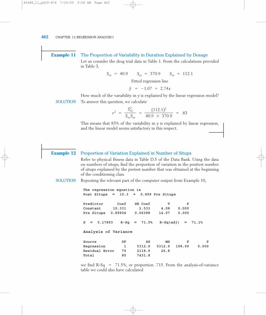
Example 11 The Proportion of Variability in Duration Explained by DosageLet us consider the drug trial data in Table 1. From the calculations providedin Table 3,
Fitted regression line
How much of the variability in y is explained by the linear regression model?
SOLUTION To answer this question, we calculate
This means that 83% of the variability in y is explained by linear regression,and the linear model seems satisfactory in this respect.
Example 12 Proportion of Variation Explained in Number of SitupsRefer to physical fitness data in Table D.5 of the Data Bank. Using the dataon numbers of situps, find the proportion of variation in the posttest numberof situps explained by the pretest number that was obtained at the beginningof the conditioning class.
SOLUTION Repeating the relevant part of the computer output from Example 10,
The regression equation isPost Situps � 10.3 � 0.899 Pre Situps
Predictor Coef SE Coef T PConstant 10.331 2.533 4.08 0.000Pre Situps 0.89904 0.06388 14.07 0.000
S � 5.17893 R-Sq � 71.5% R-Sq(adj) � 71.1%
Analysis of Variance
Source DF SS MS F PRegression 1 5312.9 5312.9 198.09 0.000Residual Error 79 2118.9 26.8Total 80 7431.8
we find R-Sq � 71.5%, or proportion .715. From the analysis-of-variancetable we could also have calculated
r 2 �Sxy
2
SxxSyy�
(112.1)2
40.9 � 370.9� .83
y � �1.07 � 2.74x
Sxx � 40.9 Syy � 370.9 Sxy � 112.1
45688_11_p429-474 7/25/05 9:58 AM Page 462

Using a person’s pretest number of situps to predict their posttest number ofsitups explains that 71.5% of the variation is the posttest number.
When the value of r 2 is small, we can only conclude that a straight line rela-tion does not give a good fit to the data. Such a case may arise due to thefollowing reasons.
1. There is little relation between the variables in the sense that the scatterdiagram fails to exhibit any pattern, as illustrated in Figure 9a. In thiscase, the use of a different regression model is not likely to reduce theSSE or explain a substantial part of Syy .
2. There is a prominent relation but it is nonlinear in nature; that is, thescatter is banded around a curve rather than a line. The part of Syy thatis explained by straight line regression is small because the model isinappropriate. Some other relationship may improve the fit substan-tially. Figure 9b illustrates such a case, where the SSE can be reduced byfitting a suitable curve to the data.
Sum of squares regressionTotal sum of squares
�5312.97431.8
� .715
7. THE STRENGTH OF A LINEAR RELATION 463
y
x(a)
y
x(b)
Figure 9 Scatter diagram patterns:(a) No relation. (b) A nonlinear relation.
45688_11_p429-474 7/25/05 9:58 AM Page 463
464 CHAPTER 11/REGRESSION ANALYSIS I
Exercises
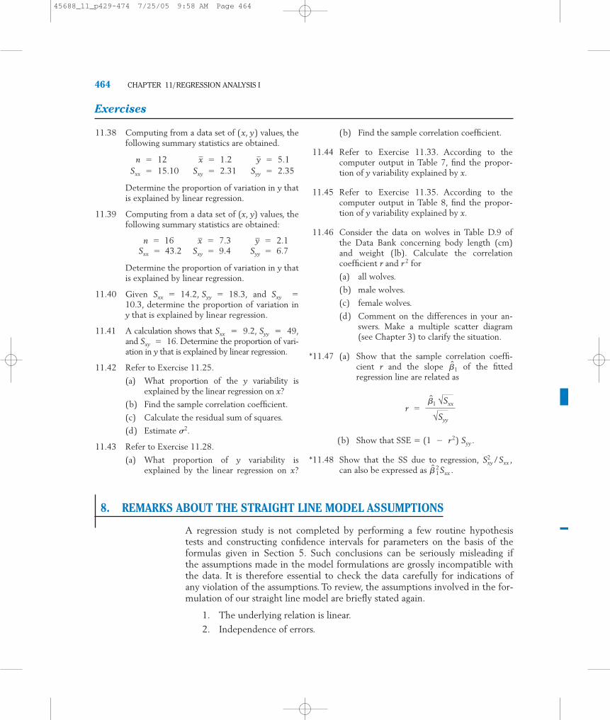
11.38 Computing from a data set of (x, y) values, thefollowing summary statistics are obtained.
Determine the proportion of variation in y thatis explained by linear regression.
11.39 Computing from a data set of (x, y) values, thefollowing summary statistics are obtained:
n � 16Sxx � 43.2 Sxy � 9.4 Syy � 6.7
Determine the proportion of variation in y thatis explained by linear regression.
11.40 Given and Sxy �10.3, determine the proportion of variation iny that is explained by linear regression.
11.41 A calculation shows that Sxx � 9.2, Syy � 49,and Sxy � 16. Determine the proportion of vari-ation in y that is explained by linear regression.
11.42 Refer to Exercise 11.25.
(a) What proportion of the y variability isexplained by the linear regression on x?
(b) Find the sample correlation coefficient.
(c) Calculate the residual sum of squares.
(d) Estimate �2.
11.43 Refer to Exercise 11.28.
(a) What proportion of y variability isexplained by the linear regression on x?
Sxx � 14.2, Syy � 18.3,
y � 2.1x � 7.3
Sxx � 15.10 Sxy � 2.31 Syy � 2.35 n � 12 x � 1.2 y � 5.1
(b) Find the sample correlation coefficient.
11.44 Refer to Exercise 11.33. According to thecomputer output in Table 7, find the propor-tion of y variability explained by x.
11.45 Refer to Exercise 11.35. According to thecomputer output in Table 8, find the propor-tion of y variability explained by x.
11.46 Consider the data on wolves in Table D.9 ofthe Data Bank concerning body length (cm)and weight (lb). Calculate the correlationcoefficient r and r 2 for
(a) all wolves.
(b) male wolves.
(c) female wolves.
(d) Comment on the differences in your an-swers. Make a multiple scatter diagram(see Chapter 3) to clarify the situation.
*11.47 (a) Show that the sample correlation coeffi-cient r and the slope of the fittedregression line are related as
(b) Show that SSE � (1 � r2) Syy .
*11.48 Show that the SS due to regression,can also be expressed as � 1
2Sxx .Sxy
2 / Sxx ,
r ��1 √Sxx
√Syy
�1
8. REMARKS ABOUT THE STRAIGHT LINE MODEL ASSUMPTIONS
A regression study is not completed by performing a few routine hypothesistests and constructing confidence intervals for parameters on the basis of theformulas given in Section 5. Such conclusions can be seriously misleading ifthe assumptions made in the model formulations are grossly incompatible withthe data. It is therefore essential to check the data carefully for indications ofany violation of the assumptions. To review, the assumptions involved in the for-mulation of our straight line model are briefly stated again.
1. The underlying relation is linear.
2. Independence of errors.
45688_11_p429-474 7/25/05 9:58 AM Page 464

KEY IDEAS AND FORMULAS 465
3. Constant variance.
4. Normal distribution.
Of course, when the general nature of the relationship between y andx forms a curve rather than a straight line, the prediction obtained from fit-ting a straight line model to the data may produce nonsensical results. Often,a suitable transformation of the data reduces a nonlinear relation to one thatis approximately linear in form. A few simple transformations are discussed inChapter 12. Violating the assumption of independence is perhaps the mostserious matter, because this can drastically distort the conclusions drawn fromthe t tests and the confidence statements associated with interval estimation.The implications of assumptions 3 and 4 were illustrated earlier in Figure 3.If the scatter diagram shows different amounts of variability in the yvalues for different levels of x, then the assumption of constant variance mayhave been violated. Here, again, an appropriate transformation of the dataoften helps to stabilize the variance. Finally, using the t distribution inhypothesis testing and confidence interval estimation is valid as long as theerrors are approximately normally distributed. A moderate departure fromnormality does not impair the conclusions, especially when the data set islarge. In other words, a violation of assumption 4 alone is not as serious as aviolation of any of the other assumptions. Methods of checking the residualsto detect any serious violation of the model assumptions are discussed inChapter 12.
USING STATISTICS WISELY
1. As a first step, plot the response variable versus the predictor variable.Examine the plot to see if a linear or other relationship exists.
2. Apply the principal of least squares to obtain estimates of the coeffi-cients when fitting a straight line model.
3. Determine the 100(1 � )% confidence intervals for the slope and in-tercept parameters. You can also look at P–values to decide whether ornot they are non-zero. If not, you can use the fitted line for prediction.
4. Don’t use the fitted line to make predictions beyond the range of thedata. The model may be different over that range.
KEY IDEAS AND FORMULAS
In its simplest form, regression analysis deals with studying the manner inwhich the response variable y depends on a predictor variable x. Sometimes,the response variable is called the dependent variable and predictor variable iscalled the independent or input variable.
45688_11_p429-474 7/25/05 9:58 AM Page 465

466 CHAPTER 11/REGRESSION ANALYSIS I
The first important step in studying the relation between the variables y and xis to plot the scatter diagram of the data (xi , yi), i � 1, . . . , n. If this plot indi-cates an approximate linear relation, a straight line regression model is formulated:
Yi � �0 � �1xi � ei
The random errors are assumed to be independent, normally distributed, andhave mean 0 and equal standard deviations �.
The least squares estimate of and least squares estimate of areobtained by the method of least squares, which minimizes the sum of squareddeviations � The least squares estimates and deter-mine the best fitting regression line which serves to predict yfrom x.
The differences Observed response � Predicted response arecalled the residuals.
The adequacy of a straight line fit is measured by r2, which represents theproportion of y variability that is explained by the linear relation between y andx. A low value of r2 only indicates that a linear relation is not appropriate—there may still be a relation on a curve.
Least squares estimators
Best fitting straight line
Residuals
Residual sum of squares
Estimate of variance �2
Inferences1. Inferences concerning the slope �1 are based on the
and the sampling distribution
Estimated S.E. �S
√Sxx
Estimator �1
S2 �SSE
n � 2
SSE � �n
i � 1 e i
2 � Syy �Sxy
2
Sxx
e i � yi � y i � yi � �0 � �1 xi
y � �0 � �1 x
�1 �Sxy
Sxx �0 � y � �1 x
yi � y i �
y � �0 � �1x,�1�0( yi � �0 � �1xi )
2.
�1�0
Response � A straight line in x � Random error
45688_11_p429-474 7/25/05 9:58 AM Page 466
A 100(1 � )% confidence interval for �1 is
To test H0��1 � �10 , the test statistic is
2. Inferences concerning the intercept �0 are based on the
and the sampling distribution
A 100(1 � )% confidence interval for �0 is
3. At a specified the expected response is �0 � �1x*. Inferencesabout the expected response are based on the
A 100(1 � )% confidence interval for the expected response at x* isgiven by
4. A single response at a specified is predicted by with
Estimated S.E. � S �1 �1n
�(x* � x )2
Sxx
�0 � �1x*x � x*
�0 � �1x* � t/2 S � 1n
�(x* � x )2
Sxx
Estimated S.E. � S � 1n
�(x* � x )2
Sxx
Estimator �0 � �1x*
x � x*,
�0 � t/2 S � 1n
�x2
Sxx
T ��0 � �0
S � 1n
�x2
Sxx
d.f. � n � 2
Estimated S.E. � S � 1n
�x2
Sxx
Estimator �0
T ��1 � �10
S / √Sxx
d.f. � n � 2
�1 � t/2 S
√Sxx
T ��1 � �1
S / √Sxx
d.f. � n � 2
KEY IDEAS AND FORMULAS 467
45688_11_p429-474 7/25/05 9:58 AM Page 467

468 CHAPTER 11/REGRESSION ANALYSIS I
A 100(1 � �)% prediction interval for a single response is
Decomposition of Variability
The total sum of squares Syy is the sum of two components, the sum of squaresdue to regression and the sum of squares due to error
Variability explained by the linear relation �
Residual or unexplained variability � SSE
Total y variability � Syy
The strength of a linear relation, or proportion of y variability explained bylinear regression
Sample correlation coefficient
TECHNOLOGY
Fitting a straight line and calculating the correlation coefficient
MINITAB
Fitting a straight line—regression analysis
Begin with the values for the predictor variable x in C1 and the response vari-able y in C2.
Stat � Regression � Regression.Type C2 in Response. Type C1 in Predictors.Click OK.
To calculate the correlation coefficient, start as above with data in C1 and C2.
Stat � Basic Statistics � Correlation.Type C1 C2 in Variables. Click OK.
r �Sxy
√Sxx Syy
r 2 �Sxy
2
Sxx Syy
Sxy2
Sxx� � 1
2Sxx
Syy �S2
xy
Sxx� SSE
S2xy /Sxx
�0 � �1x* � t�/2 S �1 �1n
�(x* � x )2
Sxx
45688_11_p429-474 7/27/05 3:08 PM Page 468

TECHNOLOGY 469
EXCEL
Fitting a straight line—regression analysis
Begin with the values of the predictor variable in column A and the values ofthe response variable in column B. To plot,
Highlight the data and go to Insert and then Chart.Select XY(Scatter) and click Finish.Go to Chart and then Add Trendline.Click on the Options tab and check Display equation on chart.Click OK.
To obtain a more complete statistical analysis and diagnostic plots, instead usethe following steps:
Select Tools and then Data Analysis.Select Regression. Click OK.With the cursor in the Y Range, highlight the data in column B.With the cursor in the X Range, highlight the data in column A.Check boxes for Residuals, Residual Plots, and Line Fit Plot. Click OK.
To calculate the correlation coefficient, begin with the first variable in column Aand the second in column B.
Click on a blank cell. Select Insert and then Function(or click on the fx icon).Select Statistical and then CORREL.Highlight the data in column A for Array1 and highlight the data in column Bfor Array2. Click OK.
TI-84/-83 PLUS
Fitting a straight line—regression analysis
Enter the values of the predictor variable in L1 and those of the response vari-able in L2.
Select STAT, then CALC, and then 4�LinReg (ax � b).With LinReg on the Home screen Press Enter.
The calculator will return the intercept a, slope b, and correlation coefficient r.If r is not shown, go to the 2nd 0 :CATALOG and select Diagnostic. PressENTER twice. Then go back to LinReg.
45688_11_p429-474 7/25/05 9:58 AM Page 469

470 CHAPTER 11/REGRESSION ANALYSIS I
9. REVIEW EXERCISES
11.49 Concerns that were raised for the environmentnear a government facility led to a study ofplants. Since leaf area is difficult to measure,the leaf area (cm2) was fit to
using a least squares approach. For data collectedone year, the fitted regression line is
and Comment on the size of theslope. Should it be positive or negative, lessthan one, equal to one, or greater than one?
11.50 Given these nine pairs of (x, y) values:
x 1 1 1 2 3 3 4 5 5
y 9 7 8 10 15 12 19 24 21
(a) Plot the scatter diagram.
(b) Calculate and
(c) Determine the equation of the leastsquares fitted line and draw the line onthe scatter diagram.
(d) Find the predicted y corresponding to
11.51 Refer to Exercise 11.50.
(a) Find the residuals.
(b) Calculate the SSE by (i) summing thesquares of the residuals and also (ii) usingthe formula SSE �
(c) Estimate the error variance.
11.52 Refer to Exercise 11.50.
(a) Construct a 95% confidence interval forthe slope of the regression line.
(b) Obtain a 90% confidence interval forthe expected y value corresponding to
11.53 An experiment is conducted to determine howthe strength y of plastic fiber depends on thesize x of the droplets of a mixing polymer insuspension. Data of (x, y) values, obtained
x � 4.
Syy � Sxy2 / Sxx .
x � 3.
Sxy .x, y, Sxx , Syy ,
s2 � (0.3)2.
y � .2 � 0.5x
x � Leaf length � Leaf width
from 15 runs of the experiment, have yieldedthe following summary statistics.
(a) Obtain the equation of the least squaresregression line.
(b) Test the null hypothesis H0��1 � �2against the alternative H1��1 � �2,with � � .05.
(c) Estimate the expected fiber strength fordroplet size x � 10 and set a 95% confi-dence interval.
11.54 Refer to Exercise 11.53.
(a) Obtain the decomposition of the totaly variability into two parts: one explainedby linear relation and one not explained.
(b) What proportion of the y variability isexplained by the straight line regression?
(c) Calculate the sample correlation coeffi-cient between x and y.
11.55 A recent graduate moving to a new job col-lected a sample of monthly rent (dollars) andsize (square feet) of 2-bedroom apartments inone area of a midwest city.
Sxx � 5.6 Sxy � �12.4 Syy � 38.7y � 54.8x � 8.3
(a) Plot the scatter diagram and find the leastsquares fit of a straight line.
(b) Do these data substantiate the claim thatthe monthly rent increases with the sizeof the apartment? (Test with � � .05).
(c) Give a 95% confidence interval for theexpected increase in rent for one addi-tional square foot.
(d) Give a 95% prediction interval for themonthly rent of a specific apartment hav-ing 1025 square feet.
Size Rent
900 550925 575932 620940 620
Size Rent
1000 6501033 6751050 7151100 840
45688_11_p429-474 7/27/05 3:08 PM Page 470

11.56 Refer to Exercise 11.55.
(a) Calculate the sample correlation coefficient.
(b) What proportion of the y variability isexplained by the fitted regression line?
11.57 A Sunday newspaper lists the following used-car prices for a foreign compact, with age xmeasured in years and selling price y measuredin thousands of dollars.
(b) Calculate the sample correlation coeffi-cient between x and y.
(c) Comment on the adequacy of the straightline fit.
The Following Exercises Require a Computer
11.61 Using the computer. The calculations involvedin a regression analysis become increasinglytedious with larger data sets. Access to a com-puter proves to be of considerable advantage.We repeat here a computer-based analysis oflinear regression using the data of Example 4and the MINITAB package.
The sequence of steps in MINITAB:
9. REVIEW EXERCISES 471
Data: C11T3.DAT
C1: 3 3 4 5 6 6 7 8 8 9
C2: 9 5 12 9 14 16 22 18 24 22
Dialog box:
Stat Regression Regression
Type C2 in Response
Type C1 in Predictors. Click OK.
(a) Plot the scatter diagram.
(b) Determine the equation of the leastsquares regression line and draw this lineon the scatter diagram.
(c) Construct a 95% confidence interval forthe slope of the regression line.
11.58 Refer to Exercise 11.57.
(a) From the fitted regression line, determinethe predicted value for the average sellingprice of a 5-year-old car and construct a95% confidence interval.
(b) Determine the predicted value for a 5-year-old car to be listed in next week’spaper. Construct a 90% prediction interval.
(c) Is it justifiable to predict the sellingprice of a 15-year-old car from the fittedregression line? Give reasons for youranswer.
11.59 Again referring to Exercise 11.57, find the sam-ple correlation coefficient between age and sell-ing price. What proportion of the y variability isexplained by the fitted straight line? Commenton the adequacy of the straight line fit.
11.60 Given
(a) Find the equation of the least squaresregression line.
� x2 � 19 � xy � 21 � y2 � 73
n � 20 � x � 17 � y � 31
produces all the results that are basic to a lin-ear regression analysis. The important pieces inthe output are shown in Table 9.
Compare Table 9 with the calculationsillustrated in Sections 4 to 7. In particular,identify:
(a) The least squares estimates.
(b) The SSE.
(c) The estimated standard errors of and .
(d) The t statistics for testing H0 :�0 � 0and H0 :�1 � 0.
(e) r2.
(f) The decomposition of the total sum ofsquares into the sum of squares explainedby the linear regression and the residualsum of squares.
11.62 Consider the data on all of the wolves in TableD.9 of the Data Bank concerning body length
�1�0
x y
1 16.92 12.92 13.94 13.04 8.8
x y
5 8.97 5.67 5.78 6.0
45688_11_p429-474 7/27/05 3:08 PM Page 471

472 CHAPTER 11/REGRESSION ANALYSIS I
(cm) and weight (lb). Using MINITAB orsome other software program:
(a) Plot weight versus body length.
(b) Obtain the least squares fit of weight tothe predictor variable body length.
(c) Test H0��1 � 0 versus H1��1 0 with� � .05.
11.63 Refer to Exercise 11.62 and a least squares fitusing the data on all of the wolves in TableD.9 of the Data Bank concerning body length(cm) and weight (lb). There is one obviousoutlier, row 18 with body length 123 andweight 106, indicated in the MINITAB out-put. Drop this observation.
(a) Obtain the least squares fit of weight tothe predictor variable body length.
(b) Test H0 :�1 � 0 versus H1 :�1 0 with� � .05.
(c) Comment on any important differencesbetween your answers to parts (a) and (b)and the answer to Exercise 11.62.
11.64 Many college students obtain college degreecredits by demonstrating their proficiency onexams developed as part of the College LevelExamination Program (CLEP). Based on theirscores on the College Qualification Test(CQT), it would be helpful if students couldpredict their scores on a corresponding portion
of the CLEP exam. The following data (cour-tesy of R. W. Johnson) are for Total CQTscore and Mathematical CLEP score.y �
x �
TABLE 9 MINITAB Regression Analysis of the Data in Example 4
THE REGRESSION EQUATION ISY � �1.07 � 2.74x
PREDICTOR COEF STDEV T-RATIO PCONSTANT �1.071 2.751 �0.39 0.707X 2.7408 0.4411 6.21 0.000
S � 2.821 R-SQ � 82.8%
ANALYSIS OF VARIANCE
SOURCE DF SS MS F PREGRESSION 1 307.25 307.25 38.62 0.000ERROR 8 63.65 7.96TOTAL 9 370.90
(a) Find the least squares fit of a straight line.
(b) Construct a 95% confidence interval forthe slope.
(c) Construct a 95% prediction interval forthe CLEP score of a student who obtainsa CQT score of 150.
(d) Repeat part (c) with and
11.65 Crickets make a chirping sound with their wingcovers. Scientists have recognized that there isa relationship between the frequency of chirpsand the temperature. (There is some truth tothe cartoon on p. 432.) Use the 15 measure-ments for the striped ground cricket to:
x � 195.x � 175
x y
170 698147 518166 725125 485182 745133 538146 485125 625136 471179 798
x y
174 645128 578152 625157 558174 698185 745171 611102 458150 538192 778
45688_11_p429-474 7/27/05 3:08 PM Page 472
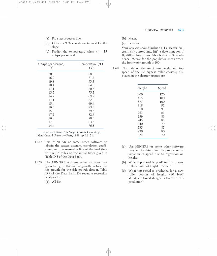
11.66 Use MINITAB or some other software toobtain the scatter diagram, correlation coeffi-cient, and the regression line of the final timeto run 1.5 miles on the initial times given inTable D.5 of the Data Bank.
11.67 Use MINITAB or some other software pro-gram to regress the marine growth on freshwa-ter growth for the fish growth data in TableD.7 of the Data Bank. Do separate regressionanalyses for:
(a) All fish.
(b) Males.
(c) Females.
Your analysis should include (i) a scatter dia-gram, (ii) a fitted line, (iii) a determination if�1 differs from zero. Also find a 95% confi-dence interval for the population mean whenthe freshwater growth is 100.
11.68 The data on the maximum height and topspeed of the 12 highest roller coasters, dis-played in the chapter opener, are
(a) Use MINITAB or some other softwareprogram to determine the proportion ofvariation in speed due to regression onheight.
(b) What top speed is predicted for a newroller coaster of height 325 feet?
(c) What top speed is predicted for a newroller coaster of height 480 feet?What additional danger is there in thisprediction?
9. REVIEW EXERCISES 473
Chirps (per second) Temperature (°F)(x) (y)
20.0 88.616.0 71.619.8 93.318.4 84.317.1 80.615.5 75.214.7 69.717.1 82.015.4 69.416.3 83.315.0 79.617.2 82.616.0 80.617.0 83.514.4 76.3
Source: G. Pierce, The Songs of Insects, Cambridge,MA: Harvard University Press, 1949, pp. 12–21.
Height Speed
400 120415 100377 100318 95310 93263 81259 81245 85240 79235 85230 80224 70
(a) Fit a least squares line.
(b) Obtain a 95% confidence interval for theslope.
(c) Predict the temperature when chirps per second.
x � 15
45688_11_p429-474 7/27/05 3:08 PM Page 473

45688_11_p429-474 7/25/05 9:59 AM Page 474