Embed Size (px)
Citation preview
1
Signaling, Screening, and
Sequential Equilibrium
Chapter 10
2
2-Player Signaling Games
Informed and uninformed playersLet the buyer bewareThree varieties of market failure, and one variety of market success

3
Two-Player Signaling GamesA good item is worth V to the buyer A bad item is worth W to the buyer
Any item, either good or bad, is offered at price p
V > p > W
The seller of a bad item must pay a cleanup cost, c
4
Caveat Emptor, extensive form
0
p, V - p
0, 0p - c, W - p
-c, 0
0, 0
0, 0
1
1
2
p(good)
p(bad)
Offer for sale
Offer for sale
Stop
Stop
Yes
Yes
No
No
g
b
5
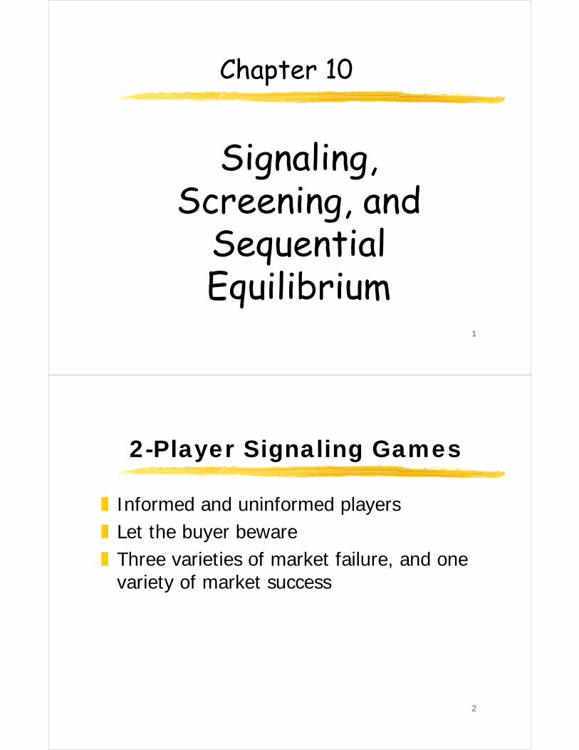
Caveat Emptor, playing the game
Price of the car: $4000
Value: good car (red card) $6000bad car (black card) $3000
Clean-up cost: $2000
6
Caveat Emptor, action sheet
Name:
3
4
action taken
5
2
1
payoffgood/bad

7
Total Market Failure
All sellers, even the good-type sellers, fearing rejection by the buyers, withhold their goods from the market. The market ceases to function, even though gains from trade are available. An equilibrium where all informed players do the same thing is called a pooling equilibrium. Total market failure is an especially sinister pooling equilibrium.
8
Total Market Success
Only sellers with good items offer them for sale. Since all items offered for sale are good, buyers buy everything offered for sale and the market works perfectly. An equilibrium where the types of informed players do different thing is called a separating equilibrium. Here, the very act of offering the item for sale signals to the buyer that it is a good type.
9
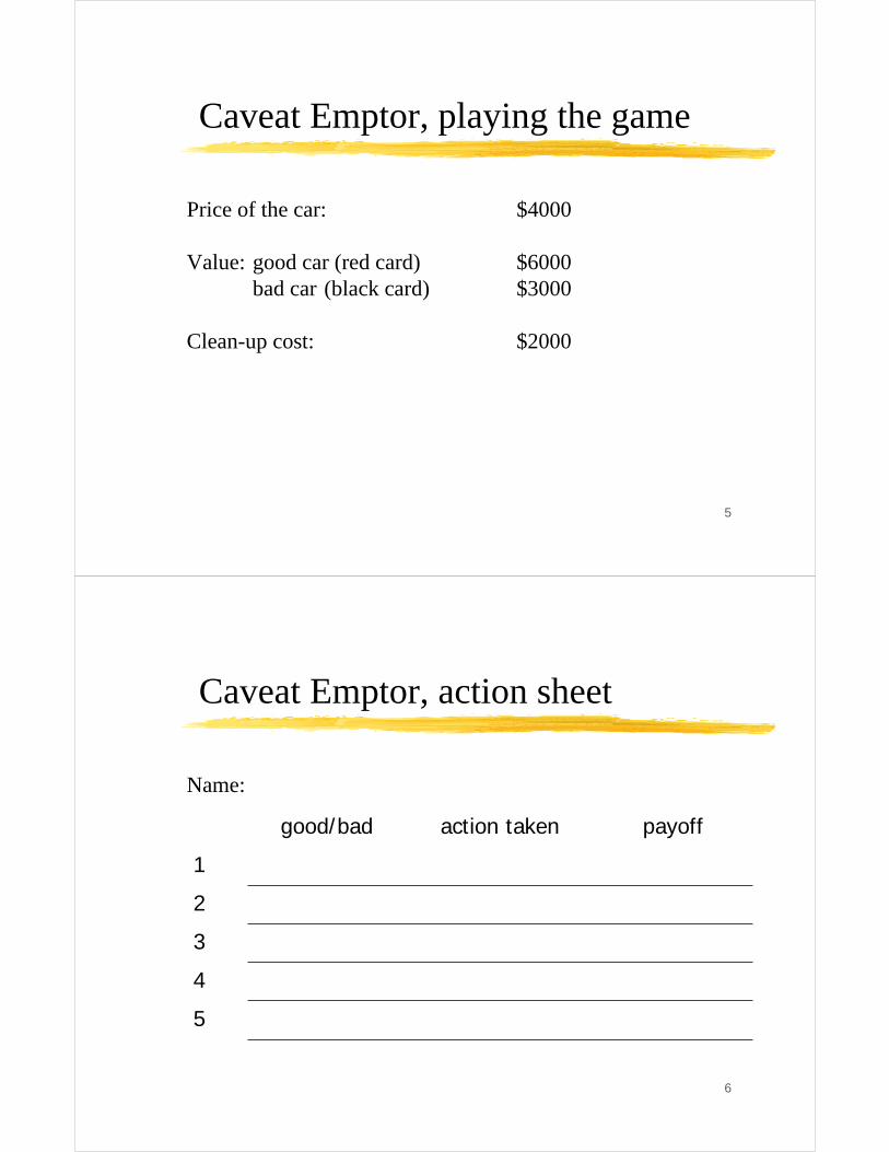
Partial Market Success
All sellers offer their items for sale, good or bad. All buyers buy whatever is offered for sale. This is only a partial success: the market functions, but there are a lot of bad deals, which reduces market efficiency. This is another example of pooling equilibrium. Unlike total market failure, however, this pooling equilibrium does generate some gains from trade.
10
Near Market Failure
Some, but not all, bad-type sellers offer their items for sale. Buyers buy what is offered for sale with a certain probability, and reject what is offered with some probability. Thus, both buyers and bad-type sellers adopt a mixed strategy response to the imperfect information. In this market, total gains from trade are smaller than in complete or partial market success.

11
Sequential Equilibrium: Pure Strategies
Sequential equilibrium as an extension of subgame perfect equilibriumSequential equilibria that pool informed playersSequential equilibria that separate informed players
12
Partial market success, reaching player 2’s information set
0
1
1
2
p(good)
p(bad)
Offer for sale
Offer for sale
Stop
Stop
g
b
13
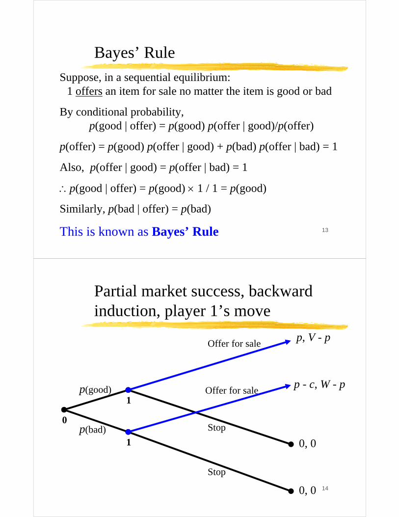
Bayes’ Rule
Suppose, in a sequential equilibrium:1 offers an item for sale no matter the item is good or bad
By conditional probability,p(good | offer) = p(good) p(offer | good)/p(offer)
p(offer) = p(good) p(offer | good) + p(bad) p(offer | bad) = 1
Also, p(offer | good) = p(offer | bad) = 1
∴p(good | offer) = p(good) × 1 / 1 = p(good)
Similarly, p(bad | offer) = p(bad)
This is known as Bayes’ Rule
14
Partial market success, backward induction, player 1’s move
0
1
1
p(good)
p(bad)
Offer for sale
Offer for sale
Stop
Stop
p, V - p
p - c, W - p
0, 0
0, 0

15
Sequential equilibrium when p > c
The following is a sequential equilibrium:1 offers the item for sale if it is good1 offers the item for sale if it is bad 2 buys whatever that is offered for sale
p(node g | offer) = p(good) and p(node b | offer) = p(bad)
p(node g | offer) = p(good | offer) / (p(good | offer) + p(bad | offer)) = p(good) / (p(good) + p(bad)) = p(good)
Similarly, p(node b | offer) = p(bad)
16
Sequential equilibrium when p > c
Eu2 = p(node g | offer) (V - p) + p(node b | offer) (W - p) = p(good | offer) (V - p) + p(bad | offer) (W - p) = p(good) (V - p) + p(bad) (W - p)
Require p(good) (V - p) + p(bad) (W - p) > 0
∴ p(good) must be sufficiently large.
This is partial market success

17
Complete market success, reaching player 2’s information set
0
1
1
2
p(good)
p(bad)
Offer for sale
Offer for sale
Stop
Stop
g
b
0, 0
0, 0
18
Complete market success, backward induction, player 1’s move
0
1
1
p(good)
p(bad)
Offer for sale
Offer for sale
Stop
Stop
p, V - p
0, 0
0, 0
p - c, W - p

19
Sequential equilibrium when c > p
The following is a sequential equilibrium:1 offers the item for sale if it is good1 stops if the item is bad2 buys whatever that is offered for sale
p(node g | offer) = 1 and p(node b | offer) = 0
p(node g | offer) = p(good | offer) = p(good) × p(offer | good) / p(offer)= p(good) / p(offer)
p(offer) = p(good) × p(offer | good) + p(bad) × p(offer | bad) = p(good) ⇒ p(node g | offer) = p(good) / p(good) = 1
Similarly, p(node b | offer) = p(bad | offer) = 0
20
Sequential equilibrium when c > p
Eu2 = p(node g | offer) (V - p) + p(node b | offer) (W - p)
= p(good | offer) (V - p) + p(bad | offer) (W - p)
= p(good) (V - p) + p(bad) (W - p) = 1 × (V - p) + 0 × (W - p) > 0
This is complete market success

21
Complete market failure, backward induction, player 1’s move
0
1
1
p(good)
p(bad)
Offer for sale
Offer for sale
Stop
Stop
0, 0
-c, 0
0, 0
0, 0
22
Sequential equilibrium when we have complete market failure
The following sequential equilibrium is not based on information about the items and leads to complete market failure:
1 stops whatever the item is2 says no to any item offered for sale p(node g | offer) = 0 and p(node b | offer) = 1
Eu2 = p(node g | offer) (V - p) + p(node b | offer) (W - p)
= 0 × (V - p) + 1 × (W - p) < 0
This is complete market failure

23
Sequential Equilibrium: Mixed Strategies
Sequential equilibria for markets on the verge of total failureA sequential equilibrium that partially separates and partially pools informed playersA regime diagram for sequential equilibria
24
Caveat Emptor, near market failure
0
0, 0
-1000, 0
0, 0
0, 0
1
1
2
0.5
Offer for sale
Offer for sale
Stop
Stop
Yes
Yes
No
No
g
b
0.5
1000, -2000
2000, 1000

25
Sequential equilibrium for near market failure
In this case, p > c andEu2 = p(good) (V - p) + p(bad) (W - p) < 0
Suppose, p(good) = p(bad) = .5, V = $3000, p = $2000, W = 0 and c = $1000
∴ p(good) (V - p) + p(bad) (W - p) = .5 × 1000 + .5 × -2000 < 0
The following is a sequential equilibrium:1 offers for sale if the item is good1 offers for sale with probability .5 if the item is
bad 2 buys any item with probability .5 p(node g | offer) = 2/3 and p(node b | offer) = 1/3
26
Verifying the sequential equilibrium for near market failure
p(node g | offer) = .5 / (.5 + .25) = 2/3p(node b | offer) = .25 / (.5 + .25) = 1/3
Eu2(buy | offer) = p(node g | offer) 1000 + p(node b | offer) (-2000) = 2/3 × 1000 + 1/3 × (-2000) = 0
Eu1(offer | good) = .5 × 2000 + .5 × 0 = 1000 > 0
Eu1(offer | bad) = .5 × 1000 + .5 × -1000 = 0

27
Caveat Emptor, regime diagram
Partial market success
Pr(good)(V - p) + Pr(bad)(W - p)
Complete market success
Near market failure
c
c = p
0
28
The market for Lemons
When price signals quality, and when it fails to signal qualityA market fails when only lemons are offered for saleExamples from health insurance and used cars

29
Lemons
0
p, V - p
0, 0
p - c, W - p
-c, 01
1
2
p(good)
p(bad)
High price
High price
Yes
Yes
No
No
g
b
Low price
Low price
b
gq, V - q
0, 0
0, 0
2q, W - qYes
No
No
Yes
30
The Market for LemonsIn a Market for Lemons,
A good item is worth V to the buyer A bad item is worth W to the buyer
An item is offered at either a high price p or a low price q
Where, V - q > V - p > W - q > 0 > W - p
The seller of a bad item must pay a cleanup cost, c

31
Sequential Equilibrium in a market for Lemons when c > p
The following is a sequential equilibrium:1 charges a high price with a good item1 charges a low price with a bad item2 buys any item offered for sale p(node g | high price) = 1p(node b | low price) = 1
In this case, thanks to the separating sequential equilibrium, Lemons has a complete market success solution.
32
Sequential Equilibrium in a market for Lemons when c = 0
In this case, a bad item can mimic a good item for free and price no longer indicates quality
A buyer’s expected value at either price is negative:Eu2 (buy|high price) = p(good)(V - p) + p(bad)(W - p) < 0 Eu2 (buy|low price) = p(good)(V - q) + p(bad)(W - q) < 0
In the very worst case the breaks down completely: 1 charges a low price with a good item2 does not buy at either price p(node g | low price) = p(good)p(node g | high price) = p(good)

33
The lemons principle
The bad drives everything out of the market
34
Costly Commitment as a Signaling Device
The principle of costly commitment Money-back-guarantees as costly commitments to solve the lemons problemCostly commitments in all walks of life

35
Money-Back Guarantee
0
p, V - p
0, 0P + W - V,V - p0, 0
1
1
2
p(good)
p(bad)
High price
High price
Yes
Nog
b
Low price
Low price
b
gq, V - q
0, 0
0, 0
2q, W - q
36
Sequential Equilibrium when the money-back guarantee is costly enough
The bad-type seller has to reimburse the unlucky buyer V - W
If p - W - V < 0, the following sequential equilibrium leads
to complete market success:1 charges a high price with a good item1 charges a low price with a bad item2 says yes to a high price2 says no to a low pricep(node g | high price) = 1p(node g | low price) = 0

37
Screening GamesUninformed player moves firstOffer of contracts by uninformed playerSubgame perfectionMenu of contracts to achieve full market successExistence of separating equilibrium
38
Screening game
1
0
offer contract
do not offer contract
0, 0
v, 1
0, 0
-v, 1
0, 0
0
0p(good)
p(bad)
yes
yes
no
no

39
Backwards induction in the screening game
Both buyers accept insurance contract since 1>0 for each.
Insurance company has expected value:
E(V1) = p(good)v + p(bad) (-v) = [p(good) – p(bad)]v
Hence insurance company offers contract if expected value is positive, or
p(good) > p(bad)
and does not offer contract if the expected value is negative,
p(good) < p(bad)
40
Backwards induction in the screening game
Full market success needs more complexity. Insurance company has two types of contract:
contract I: low premium, large deductible
contract II: high premium, low deductible
Then there could a subgame perfect equilibrium:
insurance offers both contract
good risk player: accept contract I, reject contract IIbad risk player: reject contract I, accept contract II
41
Barbarians at the Gate
The power of inside information in corporate takeoversBuying a corporation and buying a used car Bidding behavior that reveals an underlying signal The potential lemons problem in corporate takeovers
42
Repeated Signaling and Track RecordsNoisy signals and unknowable player typesBayesian updating during the probationary period Detailed calculations for one-period probation The trade-off between longer probation and the opportunity cost of ordinary performance

43
One-Period Probation
0
18
13
10
130
0
1Star 0.5
Win 0.9
Yes
Yes
No
Nowin
18
13
13
1
10Yes
No
No
YesOrdinary
0.5
Win 0.5
Lose 0.5
Lose 0.1
Star
Ordinary
Lose
Star
Ordinary
44
One-Period Probation
p(star) = p(ordinary) = 0.5 and discount factor = 0.95
When the prospective partner is a star performer,EV = Σ(.95)t + [.9 × 1 + .1 × 0] = .9 / (1-.95) = 18
When the prospective partner is a ordinary performer, EV = Σ(.95)t + [.5 × 1 + .5 × 0] = .5 / (1-.95) = 10
When you let the prospective partner go,EV = [.5 × (18 - 1) + .5 × (10 - 1)] = 13

45
Deciding on performance in one trial
Strategy 1: Yes no matter whatEV = [.5 × 18 + .5 × 10] = 14
Strategy 2: Yes if a win, No if a loss
p(star | win) = p(star) p(win | star) / p(win) = (.9 × .5) / .7 = 9/14p(ordinary | win) = 1 - p(star | win) = 5/14
p(star | loss) = p(star) p(loss | star) / p(loss) = (.5 × .1) / .3 = 1/6p(ordinary | loss) = 1 - p(star | loss) = 5/6
∴ EV = .7 × [9/14 × 18 + 5/14 × 10] + .3 × 13 = 14.5
46
Deciding on performance in one trial
Strategy 3: Yes if a loss, No if a win
EV = .7 × 13 + .3 × [1/6 × 18 + 5/6 × 10] = 12.5
Strategy 4: No, no matter what
EV = [.5 × (18 - 1) + .5 × (10 - 1)] = 13

47
Ten-Period Probation: ordinary performer
Number of wins
Probability
0 1 2 3 4 5 6 7 8 9 10
<.01 <.01.04 .04
.12 .12
.21 .21.25
48
Ten-Period Probation: star performer
Number of wins
Probability
0 1 2 3 4 5 6 7 8 9 10
.01
.06
.19
.39.35

49
Hit and Run: Track Records in HollywoodSony purchase of Columbia movie studioAsymmetric information in hiring directors Jon Peters and Peter Gruber Use of past performance as signal