Signal Timing Estimation Using Sample Intersection Travel

792 IEEE TRANSACTIONS ON INTELLIGENT TRANSPORTATION SYSTEMS, VOL. 13, NO. 2, JUNE 2012

Signal Timing Estimation Using SampleIntersection Travel Times

Peng Hao, Xuegang (Jeff) Ban, Kristin P. Bennett, Qiang Ji, Senior Member, IEEE, and Zhanbo Sun

Abstract—Signal timing information is important in signal oper-ations and signal/arterial performance measurement. Such infor-mation, however, may not be available for wide areas. This imposesdifficulty, particularly for real-time signal/arterial performancemeasurement and traffic information provisions that have receivedmuch attention recently. We study, in this paper, the possibilityof using intersection travel times, i.e., those collected betweenupstream and downstream locations of an intersection, to esti-mate signal timing parameters. The method contains three steps:1) cycle breaking that determines whether a new cycle starts;2) exact cycle boundary detection that determines when exactly acycle starts or ends; and 3) effective red (or green) time estimationthat estimates the actual duration of the red (or green) time.The proposed method is a combination of traffic flow theory andlearning/estimation algorithms and can be used to estimate thecycle-by-cycle signal timing parameters for a specific movementof a signal. The method is tested using data from microscopicsimulation, field experiments, and next-generation simulation withpromising results.

Index Terms—Intersection travel times, mobile sensors, nonlin-ear programming, signal performance measurement, signal timingestimation, support vector machine (SVM).

I. INTRODUCTION AND MOTIVATION

S IGNAL timing parameters, such as cycle length, numberof phases, and effective red and green times of the phases,

are important input to signal operations (such as signal coordi-nation) and signal performance measurement. For example, ex-isting methods for calculating steady-state signal performancemeasures, such as signal delays described in the HighwayCapacity Manual [1], rely on static signal timing parameters,e.g., cycle length, and effective red and green times. Recently,estimating real-time signal performance measures, such as real-time delays or queue lengths, has received more attention[2]–[4]. While most of these methods used data from fixedlocation sensors (e.g., loop detectors) such as volume andoccupancy, recent technological advances enable and promotethe rapid deployment of sensing technologies to collect arterialintersection travel times directly. These technologies include,for example, electronic toll collection (ETC) readers, Bluetooth

Manuscript received May 9, 2011; revised August 9, 2011 andOctober 26, 2011; accepted December 3, 2011. Date of publication March 12,2012; date of current version May 30, 2012. The work of P. Hao, X. Ban,and Z. Sun was supported by the U.S. National Science Foundation (NSF)under Grant CMMI-1031452. Any opinions, findings, and conclusions orrecommendations in this paper are those of the authors and do not necessarilyreflect the views of the NSF. The Associate Editor for this paper was W. Fan.

The authors are with the Rensselaer Polytechnic Institute, Troy, NY 12180USA (e-mail: [email protected]; [email protected]; [email protected]; [email protected]; [email protected]).

Color versions of one or more of the figures in this paper are available onlineat http://ieeexplore.ieee.org.

Digital Object Identifier 10.1109/TITS.2012.2187895

Mac address matching [5], wireless magnetic sensors [6], andmobile sensors such as Global Positioning System (GPS) cel-lular phones or other GPS devices [7], [8]. Ban et al. [4], [9]showed that intersection travel times can be used to estimateother real-time signal performance measures such as delaypatterns, queue lengths, and even arrival volumes. Methodsfor real-time signal performance estimation, using either fixedlocation sensor data or intersection travel times, require bothstatic and dynamic signal timing information, such as the cycleby cycle effective red (or green) times [4], [9].

In the current practice, collecting signal timing parametersdirectly from traffic signal controllers is probably trivial, par-ticularly for small-scale data collection (such as for signals ona corridor or a small network). However, collecting such infor-mation for large areas (such as a region or nationwide) directlyfrom controllers can be very challenging for several reasons.First, usually what is available is the signal timing plan sheet,which contains static signal timing information (e.g., cyclelength, etc.) but cannot tell what will exactly happen in real timecycle by cycle; transportation agencies may not collect/archiveat all those dynamic signal information. Second, signals areusually maintained and operated by multiple agencies underdifferent data collection and monitoring systems—as a result,collecting wide-area signal timing information, particularlydynamic cycle-by-cycle information, is not a trivial task. Third,even if the dynamic signal information is collected and archivedby each agency, it may not be easy for the agencies to releasethe data of large areas to a third party due to security and otherrelated concerns.

On the other hand, leading traffic information providers havealready started to provide wide-area real-time traffic informa-tion that aims to cover both freeways and arterials [10], [11].The lack of wide-area dynamic signal timing information willlikely limit the information provision for large-scale arterialnetworks. While it has been traditionally assumed that signaltiming information should be available as an input to trafficmodels, given the current increasingly large amount of inter-section travel time data, one intriguing question is can weinstead infer static and dynamic signal timing parameters fromintersection travel times, probably with the help of limited(and easily obtained) knowledge about the traffic signal? Theanswer to this question is not only scientifically interesting butis practically useful as well, particularly for traffic informationproviders who have already started to collect travel time infor-mation from various sources, as aforementioned. Based on thecommunications of the authors with researchers in the industry,they are anxious to integrate signal timing information withtheir arterial models. It seems that the most attractive way to do

1524-9050/$31.00 © 2012 IEEE

HAO et al.: SIGNAL TIMING ESTIMATION USING SAMPLE INTERSECTION TRAVEL TIMES 793

Fig. 1. Intersection delay pattern.

so is to infer signal timing information directly from the datathat they have already collected, such as travel times. In thispaper, we show that the answer to such a question is affirmativeat least for signals with constant cycle lengths.

In fact, the authors in [9] showed preliminarily that signaltiming parameters may be estimated using the intersection de-lay pattern. The delay pattern describes the delay that an imag-inary vehicle may experience when passing the intersection ata certain time. It can be viewed as a continuous approximationof the measured (discrete) delays calculated from intersectiontravel times. Fig. 1 depicts the intersection delay pattern as apiecewise linear curve at the bottom of the figure. The smallcircles along the curve indicate the measured delays fromindividual vehicles. Here, travel times are collected between anupstream location (denoted as virtual trip line (VTL) 1) and adownstream location (denoted as VTL2). The VTL concept wasinitially developed for mobile sensors [7], which could also in-dicate the locations where ETC readers or wireless sensors areinstalled. The signal timing estimation method in [9] is based onthe observation that a significant increase in the delay pattern iscorrelated with the start of the red time. By predefining a thresh-old for such an increase, the time that a new cycle starts can bedetected. By further correlating the time when the delay patternbecomes zero with the duration of the red, the effective redtime can also be estimated. The estimation method in [9], how-ever, is not very satisfactory because of the following: 1) Themethod cannot very well determine the exact start/end timesof a cycle; and 2) if the travel times are sparse, a significantdelay increase may not exist for one or multiple consecutivecycles, and the method cannot detect those “missing” cycles.

In this paper, we develop a robust signal timing estimationmethod. The method features a combination of traffic flowtheories and learning/optimization methods, which can estimatethe exact cycle start/end times and can properly detect themissing cycles if any. The method contains three major steps:1) cycle breaking estimation, which determine whether a newcycle starts; 2) exact cycle boundary detection, which detectsthe exact cycle start/end times; and 3) effective red (or green)time estimation, which estimates the duration of effective red(or green) times. Cycle breaking estimation applies the supportvector machine (SVM) technique to classify sample vehicledelays into two groups, one of which indicates the start of redtimes. The classification results are more accurate and robustcompared with the simple threshold method in [9]. Exact cycleboundary detection can be formulated as a nonlinear program

by assuming that the cycle length is constant (the effective redand green times may vary from cycle to cycle, e.g., for thecoordinated phases of actuated signals). A key feature of theexact cycle boundary estimation method is that the number ofmissing cycles can be estimated using sample delays and theSVM results. Finally, the effective red (or green) times areestimated using the method in [4] and [9] by investigating whennonsmoothness in the delay pattern happens.

The proposed signal timing estimation methods are tested insimulation and real-world data collected from next-generationsimulation (NGSIM). The results are promising for relativelyhigh penetration of travel time data (e.g., ≥10%–15%).

II. ROBUST CYCLE BREAKING METHOD

The first step for cycle parameter estimation is to detect whena cycle starts and ends. This is called “cycle breaking” in thispaper. Here, we only illustrate how cycle breaking can be donefor a particular movement of a signal, and the same procedureapplies to other movements of the signal. In this paper, wedefine the start of a cycle as the start of the red time.

Cycle breaking can be done by exploring the correlationbetween the delay pattern of a signalized intersection and thestart of the red time. This is because traffic at a signalizedintersection has some periodic features due to signal timing.These features can be reflected by the measured intersectiondelays (or travel times) under relatively high penetration ofmobile data. They can be seen via the discontinuities in thedelay pattern in Fig. 1 when red times start. Usually, the vehiclethat arrives at the end of a cycle, e.g., vehicle b, is not influencedby the signal and queues, whereas the vehicle that arrives atthe beginning of the next cycle (during the red time) has towait for the entire red time. On the other hand, if we knowthe delay pattern, the start of the red time can be inferred fromthe pattern by investigating when the discontinuity happens.For this purpose, we define a cycle breaking vehicle (CBV) asthe first sample vehicle in a cycle. The other vehicles in thiscycle are non-CBV (NCBV). CBV and NCBV are illustratedin Fig. 1. CEV in the figure stands for cycle ending vehicle,which will be defined later in this section. The CBV of a cycleis not necessarily the first vehicle actually arriving at the signalin the cycle if the penetration is not 100% (in this case, the firstvehicle may not be sampled).

Generally, the delays of vehicles should be continuouslydecreasing within a cycle and “jumping” to a higher valuewhen the next cycle starts. This implies that CBVs usuallyhave higher delays. Such a feature can be used to detectwhether a new cycle starts. In [9], e.g., a threshold is definedfor this purpose. If the delay increase between one vehicleand the previous vehicle exceeds this threshold, a new cyclestarts. However, using a single feature classifier is not robustif we consider oscillation and noise in measurements and, inparticular, low penetration rate. To improve the performance,we use two features: the arrival time difference ti − ti−1 andthe delay difference di − di−1 between two consecutively sam-pled vehicles. Here, ti is the ith sample vehicle’s arrival timeat VTL1, and di is the intersection delay of the ith samplevehicle. Fig. 2 depicts these two features for a field experiment


Fig. 2. Change in arrival time versus change in delay for different penetrationrates.

conducted in the Albany, NY, area [4] under 60% and 30%penetration rates of travel time data. In the figure, dots are forNCBVs and plus signs are for CBVs. We can see that thereis a clear margin of separation between CBVs and NCBVsusing these two features. Notice that the margins (dashed lines)in Fig. 2 are drawn manually, purely based on the data andintuition for illustration purposes. In the numerical section ofthis paper, the margins are automatically generated.

The fact that CBVs and NCBVs can be separable using thetwo features intuitively makes sense. Since the first measure isthe difference of the arrival times of two consecutively sampledvehicles, the larger this difference, the more likely that they arein two distinct cycles because the cycle length is finite. Since thesecond measure is the delay increase from the second vehicleto the first vehicle, a large value of this measure likely indicatesthe start of red time. The second measure is exactly what wasused in [9] for cycle breaking. Using either feature or a simplecombination of the two features, however, is not effective, asillustrated in Fig. 2. The vertical dashed bold line in the figureindicates the threshold in delay increase. The horizontal dashedbold line indicates the threshold in arrival times. The figureshows that even if both measures are used (e.g., a CBV needs tosatisfy at least one of the two measures), there will still be largeerrors, as indicated by the circles.

In order to produce robust results, these two features needto be combined more intelligently for cycle breaking. Here,

we use SVM, a widely used learning method, to classify aset of data points into two distinct groups [12]–[15]. Let thehistorical travel time data be denoted by (xi, yi), i = 1, . . . ,M(in total M samples). Here, xi = (ti − ti−1, di − di−1)T is adata point, and yi = ±1 is the corresponding label (yi = 1 forCBV and yi = −1 for NCBV). SVM can help divide the dataset into two groups: one for yi = 1 and the other for yi = −1using two support planes (lines in the R2 space, see Fig. 2).Let w = (w1, w2)T ∈ R2 and b be a scalar. If w and b areproperly selected, we will have wxi − b ≥ 1 for yi = 1 andwxi − b ≤ −1 for yi = −1. Then, the two support lines arewxi − b = 1 and wxi − b = −1. Notice that 1 and −1 can beused here by choosing proper scales for w and b. The distancebetween these two lines can be shown as 2/‖w‖ with ‖w‖,denoting the norm of w. If we aim to maximize the distancebetween these two support planes, (w, b) can be determined bysolving the following quadratic program [12]:

minw,b

1/2‖w‖2 s.t. yi(wxi − b) ≥ 1, i = 1, . . . ,M. (1)

Notice that yi(wxi − b) ≥ 1 is a compact form for thetwo cases of wxi − b ≥ 1 for yi = 1 and wxi − b ≤ −1 foryi = −1. Model (1) is an SVM for separable cases, i.e., sampleswith yi = 1 and yi = −1 can be completely separated. Thesamples satisfying constraint (1) at equality are exactly on oneof the two support planes—they are called support vectors. Formany cases, there is no plane that can perfectly divide the twogroups. In this case, we need to introduce an error term foreach data point, denoted as εi. The problem is then to solvethe following revised quadratic program [16]:

minw,b

1/2‖w‖2 + G

(M∑i=1

εi

)

s.t. yi(wxi − b ≥ 1 − εi, εi ≥ 0, i = 1, . . . ,M. (2)

The objective now is to minimize a weighted sum of thedistance and the error term. Here, G is a weighting factor thatcan be defined by the user; a larger G assigns a larger penaltyto the error.

We can solve the quadratic programming problem directly;the dual form of this problem is more preferable because itsconstraints are much simpler, i.e.,

mina

12

M∑i=1

M∑j=1

yiyjaiaj(xi · xj) −M∑i=1

ai

s.t.M∑i=1

yiai = 0 G ≥ ai ≥ 0. i = 1, . . . ,M. (3)

The dual model (3) is a quadratic program of a. Givenhistorical data {(xi, yi)}, we can find the Lagrange multiplier{ai} by solving (3). The ith data point (xi, yi) is a supportvector if its multiplier ai > 0 and the normal to the plane canbe calculated as

∑Mi=1 yiaixi. Then, we have yi(wxi − b) = 1

and ai > 0 if and only if (xi, yi) is a support vector. This meansthat b = wxi − (1/yi) if the corresponding ai is positive [15].The middle plane w · xi = b is then used to classify CBVs and


NCBVs. If w · xi > b (or w1(ti − ti−1) + w2(di − di−1)>b),the ith sample vehicle is recognized as a CBV. If w · xi ≤ b(or w1(ti − ti−1) + w2(di − di−1) ≤ b), the ith sample vehicleis classified as an NCBV. The CEV is defined as the samplevehicle that arrives just before a CBV. It is also the last samplevehicle in the previous cycle. The CEV in the nth cycle andthe CBV in the n + 1th cycle are called the nth cycle breakingpair. It is obvious that the cycle boundary between the nth cycleand the n + 1th cycle should be somewhere between the timeswhen these two vehicles arrived at the intersection. However,we do not know when exactly this happened. In [9], it wassimply assumed that the cycle boundary is exactly at the middlepoint of the two arrival times. We show next how the exactcycle boundaries can be detected based on some engineeringknowledge about the signal.

III. EXACT CYCLE BOUNDARY ESTIMATION

To detect the exact boundaries of cycles, further knowledgeabout the signal is needed. This is where engineering knowl-edge can play a critical role in developing specialized learningand optimization methods. Next, we show how exact cycleboundaries can be determined if the signal has a constant cyclelength. This applies to pretimed signals or the coordinatedphases of coordinated actuated signals. For pretimed signals,the cycle length and red/green times are fixed. For coordinatedand actuated signals, we have a fixed cycle length but variablered/green times for the coordinated phase. To detect exact cycleboundaries, we need to first figure out the exact times whenCBV and CEV arrive at the intersection (i.e., the stop line).

Here, we discuss normal cycles, i.e., the queue can be fullydischarged during the green time of the cycle, and oversaturatedcycles, i.e., the queue cannot be fully discharged during thegreen time of a cycle and some vehicles have to wait for anextra red time. To simplify the discussion, we assume thatan oversaturated vehicle waits only one extra red time to getthrough the intersection. See [4] for more details of thosedefinitions.

A. Arrival Time at the Stop Line

As defined in the previous section, CBV is the first samplevehicle within one cycle. If the penetration rate is 100%, eachCBV should be the first vehicle that actually arrives at the stopline after the start of red time; each CEV should be the lastvehicle that actually passes the stop line before the start of redtime. Because we can only detect the arrival times at VTL1and VTL2, we have to process them into times at the stop line.For different traffic conditions, we have different methods tocompute the arrival times at the stop line.

For normal conditions in Fig. 3(a), we show the trajectoriesof CEV and CBV using solid lines and the other vehicles usingdashed lines. The time that CEV passes the stop line (denotedas tnCEV) can be expressed as the difference between the arrivaltime at VTL2 (denoted as tnCEV2) and the free flow travel timefrom stop line to VTL2 (denoted as fftt2)

tnCEV = tnCEV2 − fftt2. (4)

Fig. 3. Arrival time at the stop line. (a) Normal condition. (b) Oversaturationcondition.

The time that CBV arrives at the stop line (denoted as tn+1CBV)

can be expressed as the difference between the arrival time atVTL1 (denoted as tn+1

CBV1) and the free flow travel time fromVTL1 to stop line (denoted as fftt1)

tn+1CBV = tn+1

CBV1 + fftt1. (5)

If the first vehicle in a cycle is not sampled, i.e., if CBV isnot the first vehicle actually in the queue, tn+1

CBV derived from(5) will be the time that a queued vehicle stops at the stop line,which still provides an upper bound for the boundary.

For oversaturation conditions, the time that the CEV passesthe stop line can still be expressed by (4), as shown in Fig. 3(b).This is because the CEV must not be oversaturated by defin-ition. However, the CBV can be an oversaturated vehicle thatstops twice in front of the stop line so that (5) cannot be appliedto compute tn+1

CBV. We have to consider the first delay D0 definedas the delay of the oversaturated vehicle if there were enoughgreen time in the nth cycle, as shown in Fig. 3(b). It is alsothe delay an oversaturated vehicle experienced during the firstcycle. In [9], we proposed a piecewise linear delay model tocalculate the intersection delay over time. If the green time ofthe nth cycle is long enough, all vehicles arriving during the nthcycle follow the same delay reduction function, for example,D = α0 − α1t. Here, t is the vehicle arrival time at VTL1, andthe positive coefficients α0 and α1 are parameterized by linearfitting (for details, see [9]). Thus, we estimate the first delay ofthe CBV by the following equation:

D0 = α0 − α1tn+1CBV1 (6)


where D0 is the estimated value of the first delay for CBV. Ifthe D0 of the CBV is positive, we can conclude that this cycleis under oversaturation and derive tn+1

CBV by

tn+1CBV = tn+1

CBV1 + fftt1 + D0. (7)

If D0 of the CBV is negative or zero, we say either of thefollowing: 1) The cycle is under normal condition; or 2) thecycle is under oversaturation, but no oversaturated vehicle issampled (e.g., due to low penetration). In either case, we cancalculate tn+1

CBV by (5) because that particular CBV is a normalvehicle.

Notice here that the derivations of tn+1CBV and tnCEV assume

a uniform arrival pattern of the intersection, which may not betrue in reality. However, since tn+1

CBV and tnCEV are only used inthis paper to provide upper and lower bounds of the exact cyclestart/end times, the numerical results in Section V show thatsuch an assumption works reasonably well. For more detaileddiscussions of the limitations of the uniform arrival assumption,one can refer to [4]. In [17], the authors also proposed amethod to partially relax the uniform arrival assumption whenestimating real-time intersection queue length.

B. Exact Cycle Boundary Estimation Without Missing Cycles

For signals with constant cycle lengths, it is possible toestimate the exact boundaries of cycles by formulating a non-linear programming model. The constant cycle length can beconsidered as a constraint of the model. The key of the modelis to observe that the boundary of the nth and n + 1th cyclesshould be located between the arrival times, at the stop line,of the cycle breaking pair, i.e., the CEV in the nth cycle andthe CBV in the n + 1th cycle. This way, each cycle breakingpair provides a constraint to the problem. To have an unbiasedestimate, we assume that the objective is to minimize thedeviation of the boundary from the middle point of the arrivaltimes of CEV and CBV. This leads to the following basic modelfor cycle boundary detection.

Basic Model:

mint0,C

1N

N∑n=1

(t0 + nC − tnCEV + tn+1

CBV

2

)2

s.t. t0 + nC ≥ tnCEV, n = 1, 2, . . . , N

t0 + nC ≤ tn+1CBV, n = 1, 2, . . . , N. (8)

Here, t0 is the start of the red time of the first cycle, C isthe fixed cycle length, and N is the number of cycle breakingpairs, indicating that the number of cycles in the basic model isN + 1. Then, t0 + nC is the end of the nth cycle (or the startof the n + 1th cycle). By solving this nonlinear programmingproblem, we can obtain the estimated cycle length and the startof the red time of each cycle. Notice that the basic model(8) and the other models developed in this section are allconvex quadratic programs that are fairly easy to solve. Wecan also easily see that the cycle boundary t0 + nC = (tnCEV +tn+1CBV/2) will be a global solution if the problem (8) is feasible.

This indicates that the heuristics developed in [9] works wellonly when (8) is feasible.

Due to data errors, it is possible that model (8) does not haveany feasible solution (which actually happens for most testingcases in Section V). In this case, it is necessary to introduceerror terms on the boundary constraints. This results in anextended model for cycle boundary detection.

Extended Model:

mint0,C,ε

1N

N∑n=1

(t0 + nC − tnCEV + tn+1

CBV

2

)2

+K

N

N∑i=n

ε2n

s.t. t0 + nC ≥ tnCEV − εn, n = 1, 2, . . . , N

t0 + nC ≤ tn+1CBV + εn, n = 1, 2, . . . , N. (9)

The error variable εi denotes the tolerance on how far thecycle boundary can deviate from the interval defined by thearrival times between the CEV (of the nth cycle) and the CBV(of the n + 1th cycle). We also introduce a weighted penaltyterm K > 0 for the error terms. In this paper, K is chosen thesame as N based on some numerical experiments on differentchoices.

The cycle boundary models (8) and (9) rely on two as-sumptions: 1) The SVM model developed previously producedsatisfactorily accurate results in terms of identifying CEVs andCBVs, and 2) the CEV and CBV can be detected for each andevery cycle. Assumption 1 depends on the penetration rate ofsample travel times. We will show later that beyond certainpenetration, SVM can always produce highly accurate results.Assumption 2, however, may not be valid, even under highpenetration due to the variation of traffic. It is thus crucial toidentify whether there are any missing cycles between a CEVand a CBV and, if yes, how many of them are missing, to applythe model (8) or (9) properly.

C. Missing Cycle Identification

Under a low penetration rate, it is possible that no vehiclein a cycle can be detected. In this case, there will be no CEVor CBV in the cycle. Sometimes, we have even more than onecycle missing between a CEV and the next CBV. It is thusimportant to detect missing cycles and identify the number ofmissing cycles before (8) or (9) can be applied.

First, we focus on the case when the cycle length C is known.Between the nth cycle breaking pairs, denote mn as the numberof missing cycles. Assume that Tn

r is the actual start of the redtime in the nth detected cycle (which is before tnCEV). Then,the actual start time of the red time of the n + 1th detectedcycle is

Tn+1r = Tn

r + C(mn + 1). (10-a)

Notice here that “n” and “n + 1” are detected cycles fromthe cycle breaking pair, which are not exactly the cycle indicesthat actually happened if there are missing cycles betweenthe cycle breaking pairs. Then, tnCEV, the arrival time of theCEV in the nth detected cycle, is between the start and end


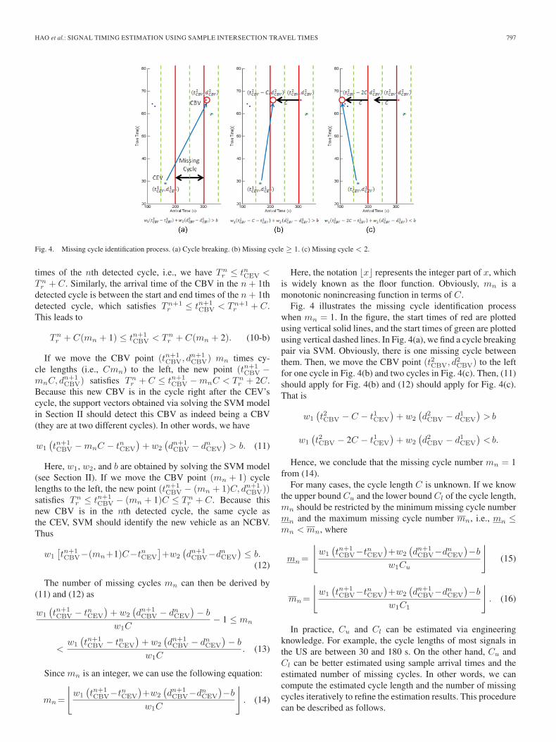
Fig. 4. Missing cycle identification process. (a) Cycle breaking. (b) Missing cycle ≥ 1. (c) Missing cycle < 2.

times of the nth detected cycle, i.e., we have Tnr ≤ tnCEV <

Tnr + C. Similarly, the arrival time of the CBV in the n + 1th

detected cycle is between the start and end times of the n + 1thdetected cycle, which satisfies Tn+1

r ≤ tn+1CBV < Tn+1

r + C.This leads to

Tnr + C(mn + 1) ≤ tn+1

CBV < Tnr + C(mn + 2). (10-b)

If we move the CBV point (tn+1CBV, dn+1

CBV) mn times cy-cle lengths (i.e., Cmn) to the left, the new point (tn+1

CBV −mnC, dn+1

CBV) satisfies Tnr + C ≤ tn+1

CBV − mnC < Tnr + 2C.

Because this new CBV is in the cycle right after the CEV’scycle, the support vectors obtained via solving the SVM modelin Section II should detect this CBV as indeed being a CBV(they are at two different cycles). In other words, we have

w1

(tn+1CBV − mnC − tnCEV

)+ w2

(dn+1CBV − dn

CEV

)> b. (11)

Here, w1, w2, and b are obtained by solving the SVM model(see Section II). If we move the CBV point (mn + 1) cyclelengths to the left, the new point (tn+1

CBV − (mn + 1)C, dn+1CBV))

satisfies Tnr ≤ tn+1

CBV − (mn + 1)C ≤ Tnr + C. Because this

new CBV is in the nth detected cycle, the same cycle asthe CEV, SVM should identify the new vehicle as an NCBV.Thus

w1

[tn+1CBV−(mn+1)C−tnCEV

]+w2

(dn+1CBV−dn

CEV

)≤ b.

(12)

The number of missing cycles mn can then be derived by(11) and (12) as

w1

(tn+1CBV − tnCEV

)+ w2

(dn+1CBV − dn

CEV

)− b

w1C− 1 ≤ mn

<w1

(tn+1CBV − tnCEV

)+ w2

(dn+1CBV − dn

CEV

)− b

w1C. (13)

Since mn is an integer, we can use the following equation:

mn =

⌊w1

(tn+1CBV−tnCEV

)+w2

(dn+1CBV−dn

CEV

)−b

w1C

⌋. (14)

Here, the notation �x� represents the integer part of x, whichis widely known as the floor function. Obviously, mn is amonotonic nonincreasing function in terms of C.

Fig. 4 illustrates the missing cycle identification processwhen mn = 1. In the figure, the start times of red are plottedusing vertical solid lines, and the start times of green are plottedusing vertical dashed lines. In Fig. 4(a), we find a cycle breakingpair via SVM. Obviously, there is one missing cycle betweenthem. Then, we move the CBV point (t2CBV, d2

CBV) to the leftfor one cycle in Fig. 4(b) and two cycles in Fig. 4(c). Then, (11)should apply for Fig. 4(b) and (12) should apply for Fig. 4(c).That is

w1

(t2CBV − C − t1CEV

)+ w2

(d2CBV − d1

CEV

)>b

w1

(t2CBV − 2C − t1CEV

)+ w2

(d2CBV − d1

CEV

)<b.

Hence, we conclude that the missing cycle number mn = 1from (14).

For many cases, the cycle length C is unknown. If we knowthe upper bound Cu and the lower bound Cl of the cycle length,mn should be restricted by the minimum missing cycle numbermn and the maximum missing cycle number mn, i.e., mn ≤mn < mn, where

mn =

⌊w1

(tn+1CBV−tnCEV

)+w2

(dn+1CBV−dn

CEV

)−b

w1Cu

⌋(15)

mn =

⌊w1

(tn+1CBV−tnCEV

)+w2

(dn+1CBV−dn

CEV

)−b

w1C1

⌋. (16)

In practice, Cu and Cl can be estimated via engineeringknowledge. For example, the cycle lengths of most signals inthe US are between 30 and 180 s. On the other hand, Cu andCl can be better estimated using sample arrival times and theestimated number of missing cycles. In other words, we cancompute the estimated cycle length and the number of missingcycles iteratively to refine the estimation results. This procedurecan be described as follows.


At the beginning of the iteration, we define the initial state

C0l = 0, C0

u = ∞, mn = 0, mn = ∞, n = 1, 2, 3, . . . N.

In the jth iteration, we check the arrival time differencebetween CEV in the nth detected cycle and CBV in the(n + k − 1)th detected cycle. When k = 1, two vehicles are inthe same cycle, i.e.,

C ≥ tnCEV − tnCBV n = 1, 2, 3, . . . N. (17)

When k > 1, because tn+k−1CEV ≤ Tn+k−1

r + C andtnCBV ≥ Tn

r

tn+k−1CEV − tnCBV ≤ Tn+k−1

r + C − Tnr

= Tnr + (k − 1)C + C

n+k−2∑i=n

mi + C − Tnr

= kC + Cn+k−2∑

i=n

mi, k = 2, 3, 4, . . .

⇒ C ≥ tn+k−1CEV − tnCBV

k +∑n+k−2

i=n mi

≥ tn+k−1CEV − tnCBV

k +∑n+k−2

i=n mj−1i

n = 1, 2, . . . N − 1, k = 2, 3, . . . N − n + 1. (18)

The lower bound of cycle length in the jth iteration shouldbe the maximum value among tnCEV − tnCBV [from (17)] andall the (tn+k−1

CEV − tnCBV/k +∑n+k−2

i=n mj−1i ) for different k’s.

Thus, mathematically, the lower bound of the cycle length atthe jth iteration Cj

i = max(Sji ), where

Sji = {tnCEV − tnCBV : n = 1, 2, . . . N}

∪{

tn+k−1CEV − tnCBV

k +∑n+k−2

i=n mj−1

: n = 1, 2 . . . N − 1, k = 2, 3 . . . N − n + 1

}.

Note that in the first iteration m0n = ∞. (tn+k−1

CEV −tnCBV/k +

∑n+k−2i=n mj−1

i ) = 0 for each k. The lower bound ofcycle length C0

l is max{tnCEV − tnCBV : n = 1, 2 . . . N}.The maximum number of missing cycles in the jth iteration

mji then should be

mjn =

⌊w1

(tn+1CBV−tnCEV

)+w2

(dn+1CBV−dn

CEV

)−b

w1Cjl

⌋. (19)

Similarly, we check the arrival time difference betweenthe CEV in the nth detected cycle and the CBV in the(n + k − 1)th detected cycle. Because tnCEV ≤ Tn

r + C andtn+k+1CBV ≥ Tn+k+1

r

tn+k+1CBV − tnCEV ≥Tn+k+1

r − Tnr −

=Tnr + (k + 1)C + C

n+k−2∑i=n

mi − Tnr

Fig. 5. Flowchart of missing cycle detection algorithm.

= kC + Cn+k∑i=n

mi, k = 1, 2, 3, 4, . . .

C ≤ tn+k+1CBV − tnCEV

k +∑n+k

i=n mi

≤ tn+k+1CBV − tnCEV

k +∑n+k

i=n mj−1i

N = 1, 2, . . . N − 2, k = 1, 2, . . . N − n. (20)

The upper bound of the cycle length in the jth itera-tion should be the minimum value among all the (tn+k+1

CBV −tnCEV/k +

∑n+ki=n mj−1

i ) for different k, i.e., Cju = max(Sj

u),where

Sju =

{tn+k+1CBV − tnCEV

k +∑n+k

i=1 mj−1i

:

n = 1, 2, . . . N − 2, k=1, 2, . . . N − n

}.

The minimum number of missing cycles in the jth iterationmj

i then should be

mjn =

⌊w1

(tn+1CBV−tnCEV

)+w2

(dn+1CBV−dn

CEV

)−b

w1Cju

⌋. (21)

We repeat the process until one of the two conditions holds.

a) The minimum number of missing cycles is equal to themaximum number of missing cycles between each cyclebreaking pair;

b) The minimum number of missing cycles is not equal tothe maximum number of missing cycles, but neither ofthem changes when the iteration proceeds.

For the first case, the minimum and maximum numbers ofmissing cycles converge to the true value. We can derive thenumber of missing cycles successfully and then apply the cycleboundary detection model in the next section. For the secondcase, the exact number of missing cycles cannot be determinedwhen the algorithm is terminated. This case only occurs whenthe penetration rate is very low. We will claim this case asa failure in the numerical test in Section V. The process ofmissing cycle detection can be illustrated using the flowchartin Fig. 5.

D. Exact Cycle Boundary Estimation With Missing Cycles

After the number of missing cycles between each cyclebreaking pair is known, we can further improve model (9). First,


define En and tn+1CBV as follows:

En =n +n−1∑i=1

mi (22-a)

tn+1CBV = tn+1

CBV − Cmn. (22-b)

Note that En and tn+1CBV can readily be calculated if the

number of missing cycles between each cycle breaking pair isknown. Then, t0 + EnC is the end of the nth detected cycle,bounded by tnCBV and tn+1

CBV. If we remove all missing cyclesbetween the nth and n + 1th detected cycles, the arrival time ofthe new CBV t

n+1CBV should still be after the end of nth detected

cycle. This leads to the following generalized model.General Model:

mint0,C,ε

1N

N∑n=1

[t0+EnC− tnCEV + t

n+1CBV

2

]+

K

N

N∑n=1

ε2n

s.t. t0 + EnC ≥ tnCEV − εn ∀n

t0 + EnC ≤ tn+1CBV + εn ∀n. (23)

The objective in (23) is to minimize the deviation from theend of the nth detected cycle to the middle point of tnCEV andtn+1CBV (i.e., tn+1

CBV − Cmn). The constraints are similar to thosein (9). Here, (23) is in exactly the same form compared to (9) byreplacing nC and tn+1

CBV in (9) with EnC and tn+1CBV, respectively,

in (23). Solving the foregoing nonlinear programming model,we can find the estimated start of the first cycle t0 and cyclelength C. Notice here that the construction of the generalmodel (23) relies on the identification of missing cycles, whichis based on engineering knowledge (about signal and delaycharacteristics) and the results of the SVM [e.g., (11) and(12)]. One might also be able to integrate the missing cycleidentification step directly into the optimization/learning modelas a pure (but likely more complex and challenging to solve)optimization/learning problem without using the foregoingengineering-knowledge-based missing-cycle identification pro-cedure. However, (23) is obviously much simpler and easierto solve. This shows the benefits of combining engineeringknowledge and optimization/learning techniques in the model-ing procedure to solve the proposed traffic problem.

IV. EFFECTIVE RED TIME ESTIMATION

The effective red times can be estimated using the signaltiming estimation method in [9]. For normal conditions, theduration of the red time is equal to the estimated delay at thestart of the red time. For oversaturation conditions, the durationof the red time is equal to the estimated delay at the start ofthe red minus the estimated first delay defined in Section III.The duration of the effective green can then be derived if theeffective red time and cycle length are known. For more detaileddescriptions, see [9]. We then summarize the signal timingparameter estimation algorithm as follows.

Signal Timing Estimation Algorithm

Step 1: Cycle breaking estimation. Calculate changes inarrival times and changes in delays of any two consec-utive sampled vehicles. Find CEVs and CBVs by usingthe SVM.

Step 2: Oversaturation identification. Calculate the first delayusing (6). Identify oversaturation if the estimated firstdelay is positive. Otherwise, the cycle is under normalcondition.

Step 3: Arrival time calculation. Compute the arrival times ofCEVs and CBVs at the stop line for both normal and over-saturation conditions using (4), (5), and (7).

Step 4: Missing cycle detection. Follow the procedure in Fig. 5and repeat until the minimum and maximum numbers ofmissing cycles converge or do not change. If the twonumbers converge, go to step 5; otherwise, go to step 7.

Step 5: Exact cycle boundary estimation. Estimate the initialstart of red, cycle length, and exact cycle boundaries usingthe general model (23).

Step 6: Effective red and green times. The effective red andgreen times can be estimated by the method in [9]. End.

Step 7: Failure. Claim that the algorithm failed to estimatesignal timing parameters.

V. NUMERICAL EXPERIMENTS

We test the signal timing estimation method in this paperusing multiple data sets, including microscopic simulation, fieldexperiment, and NGSIM. The simulation model was developedusing Paramics (a commercial traffic simulator) for the City ofFresno, CA [18], [19]; the field test was conducted in Albany,NY, for the left turn movement of an actuated (but uncoor-dinated) intersection [4]; NGSIM data were collected at thePeachtree St in Atlanta, GA, covering four pretimed intersec-tions [20]. We use the two data sets collected for the intersectionof 14th St NE and Peachtree St: one from 12:45 to 1:00 P.M.and the other from 4:00 to 4:15 P.M.. Since the field testintersection does not have a constant cycle length, the proposedexact cycle boundary method in this paper cannot apply. Wethus only apply this data set to test the cycle breaking method.The NGSIM and simulation data are used for all three steps:1) cycle breaking estimation; 2) exact cycle boundary detection;and 3) effective red (green) time estimation.

A. Cycle Breaking Estimation

Fig. 6(a)–(k) shows the cycle breaking results for the fieldtest, NGSIM data, and data sets for nine intersections in sim-ulation. For the field test data, we use the first 15-min data fortraining and the remaining 45 min for testing. Since the twoNGSIM data sets are only 15 min each, we use the data setfrom 12:45 to 1:00 P.M. as the training data set for SVM andthe data set from 4:00 to 4:15 P.M. as the testing data set. Inthe simulation, we ran the simulation for 1 h and used the first15 min as the training data and the remaining 45 min as thetesting data. The penetration rate for the results in Fig. 6 is30%. We can see that the proposed SVM-based cycle breaking


Fig. 6. Cycle breaking results. (a) Field test data, uncoordinated phase of actuated signal. (b) NGSIM data, pretimed signal. (c) Simulation 1, pretimed signal.(d) Simulation 2, uncoordinated phase of actuated signal. (e) Simulation 3, uncoordinated phase of actuated signal. (f) Simulation 4, uncoordinated phase ofactuated signal. (g) Simulation 5, uncoordinated phase of actuated signal. (h) Simulation 6, uncoordinated phase of actuated signal. (i) Simulation 7, uncoordinatedphase of actuated signal. (j) Simulation 8, uncoordinated phase of actuated signal. (k) Simulation 9, uncoordinated phase of actuated signal.

method can almost perfectly identify CBVs and NCBVs underthis penetration rate; there is only one mismatched vehicle (outof about 150 vehicles) for the field test data. We also tested

the method for other penetration rates (as low as 5%) and otherdata sets in simulation. Similar results have been obtained, andwe found that the cycle breaking method can generate a very


TABLE IPERFORMANCE OF SIGNAL TIMING ESTIMATION

accurate classification result when the penetration is relativelyhigh (e.g., >=10%–15%). The results also indicate that thecycle breaking method can apply to signals with either fixedcycle length (e.g., pretimed signals or coordinated phases of anactuated signal) or variable cycle length (e.g., for uncoordinatedphases of an actuated signal). The results clearly show thatCBVs and NCBVs are linearly separable by the two measuresused in the SVM: 1) arrival time difference and 2) delay dif-ference of two consecutively sampled vehicles (see Section II).This explains why the proposed linear SVM is effective.

B. Exact Cycle Boundary and Effective Red Time Estimation

The exact cycle boundary detection and effective red/greentime estimation are tested using two pretimed intersections: thefirst intersection in simulation [see Fig. 6(c)] and the NGSIMdata, as shown in Table I. For the simulation data, there is only1.47-s deviation in the estimated start of red time in the firstcycle. The estimated and observed cycle lengths are almost thesame. We can also compute the effective red time using linefitting, i.e., step 6 of the algorithm in Section IV. The root meansquare error (RMSE) between the observed and estimated startof red times for all the cycles is 1.632 s. We also calculated thesignal timing parameters using the method in [9], which has anRMSE of 9.593 s. For the NGSIM data, the deviation in theestimated start of red time of the first cycle is 1.9 s. The esti-mated and observed cycle lengths are almost the same: 100.0and 100.37, respectively. The RMSE between the observed andestimated start of red times for all the nine cycles is about 3 s,which is significantly smaller than that by the method in[9], which is more than 8 s. Table I shows that the methodproposed in this paper greatly outperforms the method in [9].

Fig. 7(a) shows the estimation of the exact cycle boundariesfor the simulation data for 50% penetration. The estimatedstart times of red are plotted using vertical solid lines, and theestimated start times of green are plotted using vertical dashedlines. The actual starts of red and green times are also shownin the figure using dotted lines. We depict the travel times of

Fig. 7. Signal timing estimation. (a) Simulation data (50% penetration rate).(b) NGSIM data (20% penetration rate).

CEVs by circles, CBVs by plus signs, and other vehicles bydots. Note that if there is only one vehicle in the cycle, it isconsidered as both CEV and CBV. We can see that the samplesof travel times are well split by the estimated cycle boundaries.The estimated starts of red and green times match very wellwith the actual starts of the red and green times (the RMSE isabout 1.5 s). There is one missing cycle in this case, as shown inFig. 7(a). The cycle has three vehicle arrivals, as depicted usingtriangles. None of them, however, are sampled, i.e., the sig-nal timing estimation algorithms cannot “see” their existence.Using the missing cycle detection method, we can still properlyestimate the boundaries of this cycle. Fig. 7(b) shows resultsfor the NGSIM data under 20% penetration. There are in totalnine cycles. Five of them have only one sample, which is bothCBV and CEV. There is no sample for the second and thirdcycles. The missing cycle identification algorithm shown inFig. 5 converges at mn = 2, which correctly detected these twomissing cycles. The estimated cycle boundaries also match wellwith the actual cycle boundaries, as shown in the figure—theRMSE is about 8 s. The RMSE for the NGSIM data is highersince the penetration is lower (20% instead of 50% as for thesimulation data).

We next show the impacts of the penetration rates on theestimation performance. Fig. 8(a) depicts the RMSEs of the


Fig. 8. RMSE versus penetration rate in simulation and NGSIM. (a) Simula-tion data. (b) NGSIM data.

start of red times for different penetration rates (from 10% to100% using 5% as the increment and 50 runs for each case)for the simulation. Asterisks for each penetration rate show theRMSEs for all 50 random draws. The solid line depicts theaverage RMSE for each rate, which shows a roughly decreasingtrend as the penetration rate increases. At 5%, the SVM andthe cycle boundary detection methods fail to work because thesamples are too sparse. When the penetration rate is larger than10%, relatively accurate estimation results can be achieved, andthe RMSE is about 4 s. The error decreases to around 2 s whenthe penetration rate is larger than 30%. Fig. 8(b) depicts theRMSEs of the start of red times under different penetrationrates for the NGSIM data. Similar results can be observed: theRMSEs drop from nearly 10 s to about 5 s when penetrationrates increase from 10% to 30% and then decreases to around3 s when the penetration becomes even larger (e.g., largerthan 50%).

C. Performance of Missing Cycle Identification

We performed an experiment to determine how effectivethe approach is when missing cycles occur. As mentioned

Fig. 9. Success rate versus penetration rate in simulation and NGSIM.(a) Simulation data. (b) NGSIM data.

in Section III, we say the missing cycle detection algorithmis successful if the minimum missing cycles and maximummissing cycles converge. Otherwise, the algorithm fails. Wevaried the penetration rate from 10% (5% for simulation data)to 100% and randomly simulate sample vehicle travel timesfor 50 runs under each rate. The successes rate is defined asthe ratio between the number of runs successfully applied bymissing cycle detection algorithm and the total number of runs(i.e., 50) for each penetration rate.

Fig. 9(a) depicts the success rates of the missing cycle detec-tion algorithm on simulation data. The figure shows a suddenincrease in RMSE at about 10% and below which the algorithmcannot work well. A 100% success rate can be achieved whenthe penetration rate is greater than 20%.

Fig. 9(b) depicts the success rates of the missing cycledetection algorithm for the NGSIM data. It shows that thesuccess rate is high when the penetration rate is larger than25%. When the penetration rate is greater than 35%, a 100%success rate can be obtained. The success rate for the NGSIMdata looks lower than the simulation data because the NGSIM


sample size and the number of cycles (9) are much smaller (theNGSIM testing data were only available for 15 min).

VI. CONCLUDING REMARKS

We have presented in this paper a three-step method toestimate the signal timing parameters of an arterial intersec-tion based on sample intersection travel times, including cy-cle breaking estimation, exact cycle boundary detection, andeffective red (green) time estimation. The method was based onthe correlation between critical intersection travel time patterns(such as discontinuities) and the signal timing changes (suchas the start of the red time). Cycle breaking estimation wascast as an SVM classification problem to identify the firstsample vehicle that indicates the start of a cycle (defined asthe start of the red time). The cycle breaking algorithm can beapplied to any type of signals with or without constant cyclelengths. The exact cycle boundary detection algorithm wasformulated as a nonlinear program based on the observationthat the exact cycle boundaries must lie between the arrivaltimes of CEV and CBV. The algorithm can only be applied tosignals with constant cycle lengths such as pretimed signals orthe coordinated phases of actuated signals. The effective red(green) time estimation method was based on the line fittingmethod in [9] to explore the duration of the effective red timeand the time that the delay pattern displays nonsmoothness. Thethree-step method was tested using data from simulation, a fieldtest, and NGSIM. The results show that accurate cycle breakingand cycle boundary detection results can be achieved under rel-atively high penetration of travel time data (e.g., >=10–15%).Although it can hardly be achieved in the current state of thepractice, such high penetration of intersection travel times maybe possible in the near future with the deployment of newarterial data collection techniques. The proposed method in thispaper can then be used to estimate signal timing parameters,which can be useful to conduct large-scale signal and arterialperformance measurement, particularly for those areas wherereal-time signal information or arterial data collection systemshave yet to be established or are not easy to access.

The proposed signal timing estimation approach in this pa-per, particularly the cycle breaking (SVM-based) and exactcycle boundary detection (optimization-based) methods, is acombination of transportation principles (such as how delaychanges are correlated to signal timing) and knowledge (such assignal characteristics: constant cycle or not) with optimization/learning techniques. We believe that methods based on such acombination of traffic principles/knowledge and optimization/learning can play an important role in exploring how to bestuse travel times and similar forms of data from mobile sensors[4], [8], [9] that have been increasingly available in the field.

For future research, first, it will be of great value if we canextend the current method to deal with all signal types, e.g.,the uncoordinated phases of actuated signals or even adaptivesignals. For this, the proposed method provides a general frame-work (such as the three-step process and the idea of combiningtraffic theories/principles with advanced optimization/learningtechniques) that may be extended to capture such signals. Forexample, the cycle length variable in (8), i.e., C, may be

modeled as cycle specific as Cn, which allows the cycle lengthto vary from cycle to cycle. The authors are currently workingon this problem. Second, the method proposed in this paper candirectly be applied to estimate the signal timing parameters ofa particular movement of an intersection. To obtain a completepicture of the intersection timing setting, one needs to applythe method to all movements. A synthesis procedure is thenneeded to combine the signal timing information from all sep-arate movements into a coherent phase plan. Such a procedurewill be investigated in subsequent papers. Third, the proposedmethod may be revised to estimate the optimal offset betweentwo adjacent signals. Such information is critical for signalcoordination. Forth, extending the proposed method to signaltiming design and optimization is an interesting future researchtopic. Last but not least, the proposed method also needs tobe further tested and validated using more data sets collected,particularly from real-world congested signalized intersections.The authors will pursue this direction in future research.

ACKNOWLEDGMENT

The authors would like to thank the anonymous referees fortheir insightful comments and helpful suggestions on an earlierversion of this paper.

REFERENCES

[1] Highway Capacity Manual, Transp. Res. Board (TRB): Washington, DC,2010.

[2] A. Skabardonis and N. Geroliminis, “Real-time estimation of travel timeson signalized arterials,” in Proc. 16th Int. Symp. Transp. Traffic Theory,2005, pp. 387–406.

[3] X. Liu, X. Wu, W. Ma, and H. Hu, “Real time queue length estimationfor congested signalized intersections,” Transp. Res. Part C, EmergingTechnol., vol. 17, no. 4, pp. 412–427, 2009.

[4] X. Ban, P. Hao, and Z. Sun, “Real time queue length estimation forsignalized intersections using sampled travel times,” Transp. Res. Part C,Emerging Technol., vol. 19, no. 6, pp. 1133–1156, Dec. 2011.

[5] J. S. Wasson, J. R. Sturdevant, and D. M. Bullock, “Real-time travel timeestimates using media access control address matching,” ITE J., vol. 78,no. 6, pp. 20–23, 2008.

[6] K. Kwong, R. Kavaler, R. Rajagopal, and P. Varaiya, “Arterial traveltime estimation based on vehicle re-identification using wirelessmagnetic sensors,” Transp. Res. Part C, Emerging Technol., vol. 17, no. 6,pp. 586–606, Dec. 2009.

[7] B. Hoh, M. Gruteser, R. Herring, J. Ban, D. Work, J. Herrera, andA. Bayen, “Virtual trip lines for distributed privacy-preserving trafficmonitoring,” in Proc. Int. Conf. Mobile Syst., Appl., Services, 2008,pp. 15–28.

[8] J. C. Herrera, D. B. Work, R. Herring, X. Ban, and A. Bayen, “Evaluationof traffic data obtained via GPS-enabled mobile phones: The mobile cen-tury field experiment,” Transp. Res. Part C, Emerging Technol., vol. 18,no. 4, pp. 568–583, Aug. 2009.

[9] X. Ban, R. Herring, P. Hao, and A. Bayen, “Delay pattern estimation forsignalized intersections using sampled travel times,” Transp. Res. Rec.,vol. 2130, pp. 109–119, 2009.

[10] Google, The Bright Side of Sitting in Traffic: Crowdsourcing RoadCongestion Data, Jul. 20, 2011. [Online]. Available: http://googleblog.blogspot.com/2009/08/bright-side-of-sitting-in-traffic.html

[11] Inrix, INRIX Traffic, Jul. 20, 2011. [Online]. Available: http://www.inrixtraffic.com/

[12] B. E. Boser, I. M. Guyon, and V. Vapnik, “A training algorithm for optimalmargin classifiers,” in Proc. 5th Annu. Workshop Comput. Learn. Theory,Pittsburgh, PA, 1992, pp. 144–152.

[13] C. J. C. Burges, “A tutorial on support vector machines for patternrecognition,” Data Mining Knowl. Discovery, vol. 2, no. 2, pp. 121–167,Jun. 1998.


[14] O. L. Mangasarian, “Generalized support vector machines,” in Advancesin Large Margin Classifiers, A.J. Smola, P. Bartlett, B. Schokopf, andD. Chuurmans, Eds. Cambridge, MA: MIT Press, 2000, pp. 135–146.

[15] K. P. Bennett and C. Campbell, “Support vector machines: Hype or hal-lelujah?” SIGKDD Explorations Newslett., vol. 2, no. 2, pp. 1–13, 2000.

[16] C. Cortes and V. Vapnik, “Support vector networks,” Mach. Learn.,vol. 20, no. 3, pp. 273–297, Sep. 1995.

[17] P. Hao and X. Ban, “Vehicle queue location estimation for signalizedintersections using sample travel times from mobile sensors,” submittedfor publication.

[18] H. Liu and S. Jabari, “Evaluation of corridor traffic management andplanning strategies using microsimulation: A case study,” Transp. Res.Rec., J. Transp. Res. Board, vol. 2088, pp. 26–35, 2008.

[19] “Final report of task order 3: Corridor management plan demonstration,”California Center Innov. Transp., Univ. California, Berkeley, CA, 2006.

[20] Cambridge Systematics, Summary Rep.: NGSIM Peachtree Street(Atlanta) Data Analysis (4:00 p.m. to 4:15 p.m.), 2006. Accessed onMay 8, 2011. [Online]. Available: http://ops.fhwa.dot.gov/trafficanalysistools/ngsim.htm

Peng Hao received the B.S. degree in civilengineering from Tsinghua University, Beijing,China, in 2009. He is currently working towardthe Ph.D. degree with the Department of Civil andEnvironmental Engineering, Rensselaer PolytechnicInstitute, Troy, NY.

His research interests are intelligent transportationsystems and sensor-aided modeling and simulation.His current research focuses on application of trafficflow theory and machine learning techniques (suchas support vector machines and Bayesian networks)

to transportation modeling.

Xuegang (Jeff) Ban received the M.S. degreein computer sciences and the Ph.D. degree intransportation engineering from the University ofWisconsin, Madison.

He spent three years as a Post-Doctoral Researcherwith the Institute of Transportation Studies, Uni-versity of California, Berkeley. He is currently anAssistant Professor with the Civil and EnvironmentalEngineering Department, Rensselaer Polytechnic In-stitute, Troy, NY. His research interests are in trans-portation network modeling, traffic modeling and

simulation, and intelligent transportation systems. His current research focuseson how to use mobile traffic sensors (such as Global Positioning Systems (GPS)enabled cellular phones) as traffic probes to evaluate real-time traffic systemperformances and how to systematically integrate those sensors into dynamictraffic network analysis and management. He has published over 50 papers inpeer-reviewed journals and conferences. His research has been supported bythe National Science Foundation, U.S. Department of Transportation (USDOT),Caltrans, New York State Energy Research and Development Authority, and theNew York State Department of Transportation. He now serves on the editorialboards of the Journal of Intelligent Transportation Systems and Networks andSpatial Economics.

Kristin P. Bennett received the B.S. degree in math-ematics and computer science from the University ofPuget Sound, Tacoma, WA, and the M.S. and Ph.D.degrees in computer sciences from the University ofWisconsin, Madison.

She is currently a Professor with the Mathemat-ical Sciences and Computer Science Departments,Rensselaer Polytechnic Institute, Troy, NY. She is anactive member of the machine learning, data min-ing, and operations research communities, servingas present or past Associate or Guest Editor for

ACM Transactions on Knowledge Discovery from Data, the SIAM Journal onOptimization, Naval Research Logistics, the Machine Learning Journal, theIEEE TRANSACTIONS ON NEURAL NETWORKS, and the Journal on MachineLearning Research. She served as Program Chair of the 11th ACM SpecialInterest Group on Knowledge Discovery and Data Mining International Con-ference on Knowledge Discovery and Data Mining. She has been researchingmathematical-programming approaches to machine learning such as supportvector machines since 1989. In addition, she has worked extensively on thesuccessful application of machine learning to problems in chemistry, biology,epidemiology, engineering, and business.

Qiang Ji (SM’04) received the Ph.D. degreein electrical engineering from the University ofWashington, Seattle.

He recently served as a Program Director withthe National Science Foundation (NSF), where hemanaged NSF’s computer vision and machine learn-ing programs. He also held teaching and researchpositions with the Beckman Institute, University ofIllinois at Urbana-Champaign; the Robotics Insti-tute, Carnegie Mellon University; the Department ofComputer Science, University of Nevada at Reno;

and the U.S. Air Force Research Laboratory. He is currently a Professor withthe Department of Electrical, Computer, and Systems Engineering, RensselaerPolytechnic Institute Troy, NY. He is currently serves as the Director of theRPI Intelligent Systems Laboratory. He has published over 150 papers in peer-reviewed journals and conferences. His research has been supported by majorgovernmental agencies, including NSF, the National Institutes of Health, theDefense Advanced Research Projects Agency, the Office of Naval Research,the Army Research Office, and the Air Force Office of Scientific Research, aswell as by major companies including Honda and Boeing. His research interestsare in computer vision, probabilistic graphical models, information fusion, andtheir applications in various fields.

Dr. Ji is an Editor for several related IEEE and international journals and hasserved as Chair, Technical Area Chair, and Program Committee at numerousinternational conferences/workshops.

Zhanbo Sun received the B.S. degree in civilengineering from Tsinghua University, Beijing,China, in 2009. He is currently working towardthe Ph.D. degree with the Department of Civil andEnvironmental Engineering, Rensselaer PolytechnicInstitute, Troy, NY.

His research interests are intelligent transportationsystems and traffic modeling and simulation. Hiscurrent research focuses on the modeling and privacyprotection aspects of using mobile sensors as trafficprobes.

Documents

Signal Timing Estimation Using Sample Intersection Travel