Signal Computing: Digital Signals in the Software Domain

Signal Computing:

Digital Signals in the Software Domain

Laboratory Manual: Matlab Edition

Fall 2016

Michael StiberBilin Zhang StiberUniversity of Washington Bothell18115 Campus Way NEBothell, Washington 98011

Eric C. LarsonSouthern Methodist UniversityLyle School of Engineering3145 Dyer StreetDallas, TX 75205

Copyright © 2002–2016 by Michael and Bilin Stiber and Eric C. Larson

This work is licensed under the Creative Commons Attribution-ShareAlike 4.0International License. To view a copy of this license, visithttp://creativecommons.org/licenses/by-sa/4.0/.

http://creativecommons.org/licenses/by-sa/4.0/

CONTENTS 1Contents

1 The Matlab Lab, or How to Not Teach a Programming Language 31.1 Matlab in a (Very Small) Nutshell . . . . . . . . . . . . . . . . . . . . . . . . 31.2 Trigonometric Functions and Complex Mathematics in Matlab . . . . . . . . 71.3 Representing Analog, Discrete, and Digital Signals . . . . . . . . . . . . . . . 8

2 Let’s Get Physical 102.1 Beating . . . . . . . . . . . . . . . . . . . . . . . . . . . . . . . . . . . . . . 102.2 Fourier series representation of a physical signal . . . . . . . . . . . . . . . . 11

3 Hello, Digital! 123.1 Sampling . . . . . . . . . . . . . . . . . . . . . . . . . . . . . . . . . . . . . . 123.2 Analog to Digital Conversion . . . . . . . . . . . . . . . . . . . . . . . . . . 13

4 Feed It Forward 154.1 Overview of Filtering and Matlab . . . . . . . . . . . . . . . . . . . . . . . . 15

4.1.1 From Filter Coefficients to Transfer Function and Frequency Response 174.1.2 From Zero Placement to Filter Coefficients . . . . . . . . . . . . . . . 17

4.2 Frequency Response and Pole-Zero Plots . . . . . . . . . . . . . . . . . . . . 184.3 Linearity and Cascading Filters . . . . . . . . . . . . . . . . . . . . . . . . . 19

5 Let’s Catch Some Z’s 215.1 The z-transform, Transfer Function, & Impulse Response . . . . . . . . . . . 215.2 Z-Transforms . . . . . . . . . . . . . . . . . . . . . . . . . . . . . . . . . . . 225.3 Impulse Response . . . . . . . . . . . . . . . . . . . . . . . . . . . . . . . . . 225.4 Canceling Sinusoidal Components . . . . . . . . . . . . . . . . . . . . . . . . 23

6 To Infinity and Response! 246.1 A Note About Matlab Filter Coefficients . . . . . . . . . . . . . . . . . . . . 246.2 Feedback Filters as Recurrence Relations . . . . . . . . . . . . . . . . . . . . 246.3 Telephone Touch Tone Dialing . . . . . . . . . . . . . . . . . . . . . . . . . . 25

7 Joe Fourier Was Not a Discrete Fellow 287.1 Lab Background . . . . . . . . . . . . . . . . . . . . . . . . . . . . . . . . . . 287.2 Implementing the DFT . . . . . . . . . . . . . . . . . . . . . . . . . . . . . . 287.3 The FFT in Matlab . . . . . . . . . . . . . . . . . . . . . . . . . . . . . . . . 297.4 Using the DFT . . . . . . . . . . . . . . . . . . . . . . . . . . . . . . . . . . 307.5 Spectrograms . . . . . . . . . . . . . . . . . . . . . . . . . . . . . . . . . . . 30

Signal Computing Laboratory Manual

CONTENTS 28 I’m So Compressed 32

8.1 Sound and images in MATLAB . . . . . . . . . . . . . . . . . . . . . . . . . 328.1.1 Data Types . . . . . . . . . . . . . . . . . . . . . . . . . . . . . . . . 33

8.2 Lossless image coding . . . . . . . . . . . . . . . . . . . . . . . . . . . . . . . 338.3 Lossy audio coding: DPCM . . . . . . . . . . . . . . . . . . . . . . . . . . . 348.4 Lossy image coding: JPEG . . . . . . . . . . . . . . . . . . . . . . . . . . . . 36


1 THE MATLAB LAB, OR HOW TO NOT TEACH A PROGRAMMING LANGUAGE31 The Matlab Lab, or How to Not Teach a Programming

Language

Labs in this class will make liberal use of the Matlab numerical programming environ-ment. Because this class assumes that you are an experienced computer science student,you are expected to be able to learn how to use computer tools, and how to program innew programming languages, pretty much on your own. So, the first thing you should dois check out the Matlab documentation built into the Matlab help system, or online athttp://www.mathworks.com/help/matlab/index.html. Of course, you can always searchonline for Matlab tutorials and the like. We’ll include a very brief overview of Matlab below,and then more detailed information about the code developed specifically for this class thatyou will be using.

1.1 Matlab in a (Very Small) Nutshell

The Matlab GUI environment is very similar to IDEs that you are already familiar with.As you might expect, there are some idiosyncrasies here and there, but nothing terriblyunexpected. The major areas of difference are tools and panes that have to do with viewingvariables (something in other IDEs that you’d only see when debugging a program), thecommand pane, and figure windows that open to display graphs. The first two of thesedifferences have to do with the fact that Matlab is an interpreted language/programmingenvironment. You primary area of interaction with the Matlab interpreter will be throughthe command window, with variable information panes providing views of variables and theircontents related to your interaction. It’s interesting to note that, if you want, you can runMatlab without the GUI, providing just a command line interface.

Interpreted languages have their advantages and disadvantages. One advantage is thatanything you can use as a line of code in a program you can use immediately as a commandon the command line. This lets you test code interactively and then copy it into the script orfunction you’re writing. Like any IDE, Matlab includes an editor with syntax highlightingand debugger integration.

The disadvantage is the interpreted programs are slower. In Matlab, we get around thisby using built-in functions that operate on entire vectors or arrays as single data objects.The core loops of the built-in functions are compiled for speed. If you make good use ofthose functions, Matlab code can often be as fast as completely compiled code.

Here are some things to try:

1. Immediate calculations and variables:radius = 5 % Comments start with "%"circumference = 2 * pi * radiusarea = pi * radius^2

2. Complex numbers:


http://www.mathworks.com/help/matlab/index.html

1 THE MATLAB LAB, OR HOW TO NOT TEACH A PROGRAMMING LANGUAGE4sqrt(�1)x = 7 + 14jconj(x) % complex conjugateabs(x) % magnitude (e.g., for polar representation)angle(x) % and angle for polar repreal(x)imag(x)

3. Complex exponentials:exp(j * pi)exp(j * pi/2)exp(j * pi/4)

4. Vectors:v1 = [0 1 2 3] % Four elementsv2 = [0 : 2 : 10] % like a loop (start value : increment : end value)v3 = pi * [�0.5 �0.25 0 0.25 0.5] % All operations are vectorizedexp(j * v3)mistake = v1 * v1 % a mistake; vector mult doesn't work this waydotproduct = v1 * v1' % transposing will work, if you want to do thisarrayprod = v1 .* v1 % element�by�element ops include: .+, .�, .*, ./

5. Simple plots (note that “;” suppresses outputting results to the command window —useful if that would generate massive amounts of text, or just if you want things neat):

t = [0 : 0.01 : 2*pi];x = sin(t);plot(t, x); % default plots points connected by lines in blueplot(t, x, 'r'); % change the line colorplot(t, x, 'r.'); % change the plot style; zoom in to see individual pointsxlabel('t, ms'); % X axis label (all of your plots should have this)ylabel('Mag'); % Y axis label (all of your plots should have this)title('Triangle');% Graph title (all of your plots should have this)

If you take a sequence of commands and save them in a file with an extension of .m, theresult is a script. Assuming that the script is saved in a directory in the MATLAB searchpath, you can then execute the script by just typing its name (without the .m), just as if itwere a command. If you want your code to take parameters, return a return value, and havelocal variables, start your code with a line like:function retval = funcname(parm1, parm2)

Your code is now a function. MATLAB functions can take variable numbers of argumentsand even return variable numbers of return values, but that’s getting beyond what we needright now.


1 THE MATLAB LAB, OR HOW TO NOT TEACH A PROGRAMMING LANGUAGE5Step 1.1 It’s easy to create, concatenate, extract, and modify vectors or parts of vectors.Execute the following lines of Matlab code and explain what each echoes out:a = ones(1,3)b = zeros(1,5)x = [b, a, [1:2:12]]x(7:end)length(x)x(1:2:12)

Also, explain the difference between the square bracket notation [1:2:12] and the par-enthetical notation (1:2:12).

Step 1.2 Consider the result of the following assignment:x(7:11) = pi*(1:5)

Write a single statement that will replace the odd-indexed elements of x with the constant-10 (i.e., x(1), x(3), etc).

Step 1.3 One of the side benefits of learning Matlab is that it trains you to think in termsof parallel operations — an increasingly important skill in a profession becoming dominatedby multi-core, GPU, and distributed computing. That doesn’t mean you can’t write loops inMatlab; it’s just that your code will be more concise and efficient if you can avoid that. Theefficiency arises from the fact that the vectorized Matlab commands are mostly compiled;while the loops you write are interpreted. Consider the following loop:for k=0:7,

x(k+1) = cos(k*pi/4);endx

Why is x indexed by k+1 rather than k? What happens to the length of x for each iterationof the loop? Rewrite this computation without using the loop (as in list item 5). Besides theincrease in efficiency from avoiding an interpreted loop, what other major efficiency resultsfrom this change?

Step 1.4 Consider the following code that plots a sinusoid:t = [0 : 0.01 : 1]; % time in secondsf = 5; % freq in Hertzx = sin(2*pi*f*t);plot(t, x);xlabel('Time (sec)');

Use the MATLAB editor to create a script file called firstsin.m, verify that you’vesaved it in a directory in the MATLAB path (or add that directory to the path), and testits execution by typing firstsin at the MATLAB command prompt. Note that you canalso do:


1 THE MATLAB LAB, OR HOW TO NOT TEACH A PROGRAMMING LANGUAGE6type firstsin % prints out contents of the scriptwhich firstsin % shows directory (useful when your code shadows built�ins)

If you included documentation for this script (comments at the beginning), the commandhelp firstsin would also produce useful output.

Add three lines of code to your script, so that it will plot a cosine on top of the sine in adifferent color. Use the hold function to add a plot of0.75*cos(2*pi*f*t)

to the plot. Save the plot using the MATLAB print command as a PNG file namedstep14.png by typing:print �dpng step14

You should include all plots and code snippets in your lab report, following the instruc-tions in the report rubric.

Step 1.5 You can also use Matlab to generate sounds. A pure tone is merely a sinusoid,which you already know how to generate. Let’s generate one with a frequency of 3 kHz anda duration of 1 second:T = 1.0;f = 3000;fs = 8000;t = [0 : (1/fs) : T];x = sin(2*pi*f*t);soundsc(x, fs)

The vector of numbers x are converted into a sound waveform at a certain rate, fs, calledthe sampling rate (we will learn a lot more about this in this class). In this case, the samplingrate was set to 8000 samples/second. What is the length of the vector x?

Step 1.6 Write a new function that performs the same task as the following functionwithout using any loops. Use the idea in step 1.3 and also consult the section on the find

function, relational operators, and vector logicals in the MATLAB documentation.function B = denegify(A)% DENEGIFY Replace negative elements of matrix with zeros% Usage:% B = denegify(A)%[W,H] = size(A);for i=1:W

for j=1:Hif A(i,j) < 0

B(i,j) = 0;else

B(i,j) = A(i,j);


1 THE MATLAB LAB, OR HOW TO NOT TEACH A PROGRAMMING LANGUAGE7end

endend

1.2 Trigonometric Functions and Complex Mathematics in Matlab

Step 2.1 In this step, you are asked to complete a Matlab function to synthesize a waveformin the form of:

x(t) =NX

k=1

ak cos(2⇡ft+ �k)

This is a sum of cosines, all at the same frequency but with different phases and amplitudes.Use the following function prototype to start you off:

function x = sumcos(f, phi, a, fs, dur)% SUMCOS Synthesize a sum of cosine waves% Usage:% x = sumcos(f, phi, a, fs, dur)% Returns sum of cosines at a single frequency f, sampling% rate fs, and duration dur, each with a phase phi and% amplitude a.% f = frequency (scalar)% phi = vector of phases% a = vector of amplitudes% fs = the sampling rate in Hz (scalar)% dur = total time duration of signal (scalar)

Include your code in your writeup. Additionally, include a plot of x = sumcos(20, [0

pi/4 pi/2 3*pi/2], 200, 0.25); versus time.Hint: the MATLAB length function is useful in determining the number of elements in

a vector; the size function returns both dimensions of a vector or an array.

Step 2.2 Now, let’s see how complex exponentials can simplify things. Re-implement yoursumcos function using complex exponentials. Take advantage of the fact that multiplyinga complex sinusoid ej2⇡ft by the complex amplitude aiej� will shift its phase and changeits amplitude. Thus, you should be able to create a single complex sinusoid at the givenfrequency f and then multiply it by different a * exp(j * phi) to get multiple phase shiftedcosines. Remember that we want a real value to plot; the cosine is the real part of a complexsinusoid. Include your code in your writeup and provide a plot that demonstrates that thisfunction produces the same result as the original implementation.


1 THE MATLAB LAB, OR HOW TO NOT TEACH A PROGRAMMING LANGUAGE8Step 2.3 Generate four sinusoids with the following amplitudes and phases:

x1(t) = 6 cos(2⇡(10)t� 0.5⇡) (1)x2(t) = 3 cos(2⇡(10)t+ 0.25⇡) (2)x3(t) = 2 cos(2⇡(10)t� 0.3⇡) (3)x4(t) = 8 cos(2⇡(10)t+ 0.9⇡) (4)

a. Make a single plot of all four signals together over a range of t that will generateapproximately 3 cycles. Make sure the plot includes negative time so that the phaseat t = 0 can be measured. In order to get a smooth plot make sure that your have atleast 20 samples per period of the wave. Include your plot in your writeup.

b. Verify that the phase of all four signals is correct at t = 0, and also verify that eachone has the correct maximum amplitude. Use subplot(3,2,i) to make a six-panelsubplot that puts all of these plots in the same figure, with space for two additionalplots at the bottom. Use the xlabel, ylabel, and title functions so that the readercan figure out what the plots mean; reinforce this with your report’s figure caption.(You should include the final figure, with all subplots, that results from finishing all ofthe parts of this step.)

c. Create the sum sinusoid, x5(t) = x1(t)+x2(t)+x3(t)+x4(t). Plot x5(t) over the samerange of time as used in the last plot. Include this as the lower left panel in the plotby using subplot(3,2,5).

d. Now do some complex arithmetic; create the complex amplitudes corresponding to thesinusoids xi(t): zi = Aiej�i , i = 1, 2, 3, 4, 5. Include a table in your report of the zi inpolar and rectangular form, showing Ai, �i, Re{zi}, and Im{zi}.

1.3 Representing Analog, Discrete, and Digital Signals

In our class, we will need to manipulate analog signals (real-valued signals that are functionsof continuous time), discrete signals (real-valued signals that are functions of discrete time),and digital signals (discrete-valued signals that are functions of discrete time). No needto worry about the details or these; that will become clear later. The trickiest part ofthis is representing anything other than digital signals on a digital computer, because youcan’t. So, we’ll need to employ two key elements of software design: information hiding andmake-believe.

Information hiding is used in our implementation of analog signals. We make use of theobject-oriented programming aspects of Matlab to create an AnalogSignal class. If you lookup the documentation for AnalogSignal (using doc AnalogSignal), you’ll see somethinglike figure 1.1. The key operations on these analog signals are:

• Creating an analog signal (ex: a = AnalogSignal(’sawtooth’, 2.0, 1.0, 10.0)).


1 THE MATLAB LAB, OR HOW TO NOT TEACH A PROGRAMMING LANGUAGE9

Figure 1.1: Example help screen for the AnalogSignal class. This example may be out-of-date; use the Matlab doc AnalogSignal command to get current documentation.

• Scaling an analog signal (ex: b = a * 5)

• Adding two analog signals (ex: c = a + b)

• Subtracting two analog signals (ex: d = c - a)

• Plotting an analog signal (ex: plot(d))

• Sampling an analog signal (ex: x = d.samplehold(0.1))

You will get a lot more experience working with analog signals shortly in this class, sofor the time being just play with this a bit.


2 LET’S GET PHYSICAL 102 Let’s Get Physical

In this lab, you will use Matlab to explore the effects of summing sinusoids. You will theninvestigate how a physical signal can be considered to be composed of a sum of sinusoids— its Fourier series. You will be using the Matlab AnalogSignal class and functions athttp://faculty.washington.edu/stiber/pubs/Signal-Computing/.

2.1 Beating

In this section, you will use the Matlab AnalogSignal class to simulate an analog signalgenerator. The constructor takes the following arguments:% AnalogSignal(type, amplitude, frequency, dur)% Where:% type = 'sine', 'cosine', 'square', 'sawtooth', or 'triangle'% amplitude = signal amplitude% frequency = signal frequency% dur = signal duration

Remember that, though an AnalogSignal is simulating an analog signal, in Matlab allfunctions are sampled at discrete points in time. The crufty details of this are hidden awayin the class’s implementation. Remember also that you can always plot an AnalogSignal

to see what you have; include such figures in your report

Step 1.1 Verify that you can get a triangle wave. What is the code to generate and plota triangle wave ranging from -1 to 1 Volts with a frequency of 10Hz and a duration of 1sec?

Step 1.2 Next, verify that you can generate a sine wave of 1 second duration at a frequencyof 440Hz, ranging from -1 to +1. What is the Matlab code to do this? Use the AnalogSignalsoundsc method to play this as a sound. This pitch corresponds to “standard A” on a musicalscale — A above middle C. Use the Matlab set(gca, ’XLim’, [Xmin, Xmax]) functioncall to set the X axis limits so that the waveform is apparent (i.e., you’re not just plottinga solid blob).

Step 1.3 Generate sine waves of identical range and duration, but with frequencies of 442,444, and 448 Hz. Now, generate the sums of 440Hz and each of these new signals to generatebeating akin to tuning an instrument against the 440Hz standard. Play each sum signal; canyou hear the beating? Plot each sum signal for its full 1s duration. The beating “envelope”should be obvious. What is the beat frequency in each case? How does the beat frequencyand amplitude relate to the textbook discussion of beating?


http://faculty.washington.edu/stiber/pubs/Signal-Computing/

2 LET’S GET PHYSICAL 112.2 Fourier series representation of a physical signal

Step 2.1 Recall that any periodic signal can be represented as a sum of harmonic sinusoids.The amplitude of each harmonic is known as the Fourier Series. It may at first seem likesums of sinusoids would be poor approximations of real periodic signals, but this is not thecase. We can illustrate this using a triangle wave. The formula for synthesis of a trianglewave with frequency !0 is a sum of harmonically related sine waves (its Fourier series):

x(t) =1X

k=0

0

BBB@8

⇡2

(�1)k(2k + 1)

2

| {z }amplitude

sin((2k + 1)!0t)| {z }(2k+1)th harmonic

1

CCCA

In this case, in the analog domain, we are dealing with frequencies in Hz, and so !0 = 2⇡f0.Notice that the Fourier Series of the triangle wave only uses odd harmonics (i.e., the onlynon-zero frequencies are (2k + 1)!0 = !0, 3!0, 5!0 · · · ). Also notice that resulting wave willhave zero mean because there is no “DC” term (i.e., 2k + 1 6= 0 for any integer k).

Write a Matlab script that approximates a triangle wave by summing together the first 7harmonics of its Fourier series; plot the resultant signal (i.e., use f0, 2f0, 3f0, · · · 7f0, wheref0 =10 Hz). How does this signal compare to the triangle wave computed directly in theprevious step?

Step 2.2 Another way to view a signal is in the frequency domain. For a signal expressedin terms of its Fourier series, the frequency representation is merely the coefficients of theharmonics. Write a Matlab function or script to compute and plot the spectrum of a trianglewave. You may find the MATLAB function stem useful. Note that you are not being askedto plot the triangle wave as a function of time; you should plot the amplitudes of thecomponent sinusoids as a function of those sinusoids’ frequencies (like the vertical lines intextbook figure 1.12). Use your code to plot the spectrum of the triangle wave from theprevious step (first 7 harmonics).


3 HELLO, DIGITAL! 123 Hello, Digital!

In this lab, you will investigate how capturing an analog signal for computer use — samplingand quantization — modifies the signal, seeing how the choices you make in the parametersfor sampling and quantization affect the quality of the digitized, computer signal.

3.1 Sampling

The first step in digitization is sample and hold, in which the continuous analog signal isconverted to a discrete-time analog signal (an analog signal that only changes its value atparticular points in time). You will use the samplehold method to do this:% samplehold Perform a sample and hold function on an AnalogSignal% Usage:% x = obj.samplehold(h)% where obj = AnalogSignal% h = hold time in sec (sampling interval)% x = resultant sampled AnalogSignal

Step 1.1 Create an analog sine waveform ranging from -5 to 5V with a frequency of 200Hzand a duration of 2 seconds. Produce a plot with X-axis limits set to make the waveformvisible (i.e., don’t just make a 2s plot that tries (and fails) to show 400 cycles of the sinusoid.

Step 1.2 Use the samplehold method to produce sampled versions of this signal at 300Hz,500Hz, 1000Hz, and 2000Hz. Use the Matlab subplot command, and the discreteplot

function provided with this class’s Matlab code, to plot the original and all four sampledsignals together. Clearly, the results are not the same, and none look identical to the originalsine wave. What are the two essential pieces of information about a sine wave that need tobe preserved when sampling it? Does it appear that all sampled versions are equally usefulin achieving this? Why or why not (in other words, your answer to this question should notbe just “yes” or “no”)?

Step 1.3 Let’s look at aliasing in a little more detail and with a lot more numericalprecision. You’ll recall from the text that, once we sample a signal, we have limited therange of frequencies that we can represent in our discrete signal to the range 0 !̂ ⇡,corresponding to a range of apparent frequencies in the physical world of 0 !0 !s/2(or 0 f 0 fs/2). Any frequency in the original signal above fs/2 will be aliased into therange of possible apparent frequencies. To keep things simple, we’ll stick with a sinusoid;this time, make it 10Hz with an amplitude of -1 to +1 and a duration of 1s. This will makeit easy to count cycles when plotted. Set up a figure that can hold three plots and plot thisanalog signal in the top plot.


3 HELLO, DIGITAL! 13Step 1.4 Sample this signal at 25Hz and use the discreteplot function to plot the sam-pled signal in the middle. Sample it at 15Hz and similarly plot that sampled signal at thebottom.

Step 1.5 Before examining the plots in detail, answer the following questions: For eachof the two sampling frequencies, what is the range of apparent frequencies that can berepresented? For each, will a sinusoid with f = 10Hz be aliased? If so, what will be thedigital frequency and the apparent frequency of a 10Hz sinusoid?

Step 1.6 Examine the plots and count the number of up-and-down cycles in each. Don’tworry that each cycle doesn’t look the same, or that every other cycle seems different; justcount each. You should see 10 cycles in the top graph; how many do you see in the middleand bottom? How does this compare to the theory you discussed in the previous step? Ifthere is any discrepancy, explain it.

3.2 Analog to Digital Conversion

The last step of digitization is called “analog to digital conversion,” or quantization. In thisstep, the sampled analog signal is converted to a discrete signal, with values represented byb bit integers. We will use the quant function provided with this class’s Matlab code toperform this conversion:% QUANT Quantize a sampled (discrete) signal using a prescribed% number of bits per point.% Usage:% y = quant(x,nb,out)% where y = digital signal quantized to 2^(nb) bits resolution% x = vertical points of sampled signal% nb = number of bits to use per point% out = 'raw' means output binary values: 0,...,2^(nb�1)% otherwise, set ouput value range = input value range

Step 2.1 Write a Matlab function that compares two signals by computing the signal tonoise ratio (SNR) that results from changing one into the other (by quantization). Yourfunction should do this by first computing root mean squared (RMS) error between the two.In this case, you will be comparing a sampled signal with a quantized version of it. To dothis, you should subtract the quantized signal from the sampled signal to produce a vectorof differences (errors), then square each difference value using the MATLAB .^ operator (toget squared errors), then take the mean of these squared values using the MATLAB mean

function (mean squared error — a scalar value), and finally take the square root of thatscalar result (root mean squared error). We can compute the RMS signal in a similar way,by squaring the signal values, getting the mean of those squared values, and then taking thesquare root. The final result should be a single value — the signal-to-noise ratio (SNR) in


3 HELLO, DIGITAL! 14decibels. What is in the numerator and what is in the denominator of this ratio? Note thatthis is different than what we did in the textbook, because we are now doing the computationfor a specific signal, not just figuring SNR for a possible range of signal values.

Step 2.2 Use your code to compute the SNR for a quantized sinusoid. Generate an analogsignal with with a range of 0 to 5, frequency of 10Hz, and duration 2sec. Sample it at 25Hz.Use 2, 4, 8, 12, and 16 bits quantization, and plot SNR on the Y-axis versus number ofquantization bits on the X-axis.

Step 2.3 Repeat Step 3.2 using a square waveform with the same parameters.

Step 2.4 Repeat Step 3.2 using a triangle waveform with the same parameters.

Step 2.5 As you double the number of bits used in quantization, how does the SNR change?How does this compare to what your learned from the textbook? Refer to specific featuresof your plots from Steps 3.2–3.4 to justify your answer.


4 FEED IT FORWARD 154 Feed It Forward

This lab covers the basic concepts of filtering and feedforward filters. You may have alsoheard of feedforward filters referred to as finite impulse response (FIR) filters. In this lab,we will cover the basic idea of a filter, its mathematical representation (such as the definingequation, frequency response, and transfer function), the relationship among filter coeffi-cients, zero placement, and filter type (low pass, high pass, band reject), and some basicproperties of filters.

4.1 Overview of Filtering and Matlab

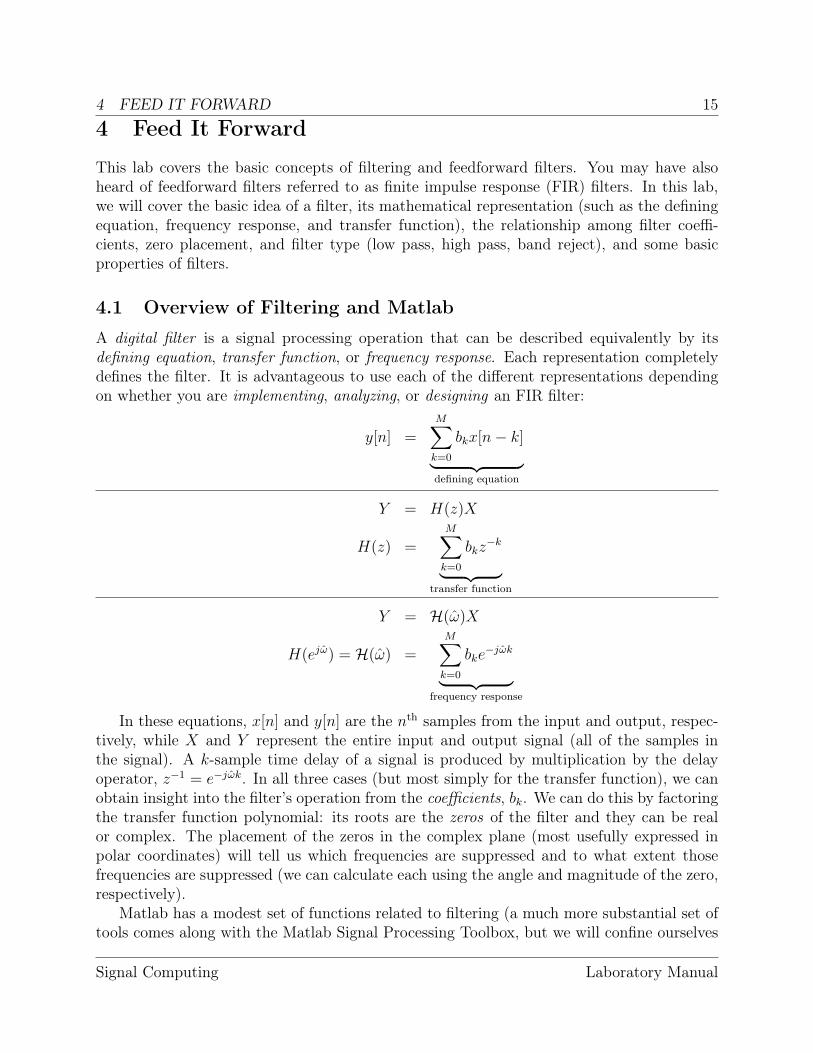
A digital filter is a signal processing operation that can be described equivalently by itsdefining equation, transfer function, or frequency response. Each representation completelydefines the filter. It is advantageous to use each of the different representations dependingon whether you are implementing, analyzing, or designing an FIR filter:

y[n] =

MX

k=0

bkx[n� k]

| {z }defining equation

Y = H(z)X

H(z) =

MX

k=0

bkz�k

| {z }transfer function

Y = H(!̂)X

H(ej!̂) = H(!̂) =

MX

k=0

bke�j!̂k

| {z }frequency response

In these equations, x[n] and y[n] are the nth samples from the input and output, respec-tively, while X and Y represent the entire input and output signal (all of the samples inthe signal). A k-sample time delay of a signal is produced by multiplication by the delayoperator, z�1

= e�j!̂k. In all three cases (but most simply for the transfer function), we canobtain insight into the filter’s operation from the coefficients, bk. We can do this by factoringthe transfer function polynomial: its roots are the zeros of the filter and they can be realor complex. The placement of the zeros in the complex plane (most usefully expressed inpolar coordinates) will tell us which frequencies are suppressed and to what extent thosefrequencies are suppressed (we can calculate each using the angle and magnitude of the zero,respectively).

Matlab has a modest set of functions related to filtering (a much more substantial set oftools comes along with the Matlab Signal Processing Toolbox, but we will confine ourselves


4 FEED IT FORWARD 16here to using core Matlab). The filter function applies a general digital filter to a signal.For this lab, we will stick using this filter as follows:a = [1]; % This will be relevant later for feedback filtersb = [b0 b1 b2]; % Coefficients (remember, Matlab indices start at 1)y = filter(b, a, x); % x is input signal; y is output

This allows us to define the bk coefficients for a filter and provide them to the filter functionas a vector so that it can filter the input signal.

We’d also like to specify a feedforward filter by indicating its zero locations, which wecan do by using the poly function to compute the coefficients from a set of roots. So, forexample, if we want a feedforward filter with zeros at 0.9+0j and 0.75e±j⇡/4, we can computethe bk values as:r = [ (0.9 + 0.0*j) (0.75*exp(j*pi/4)) (0.75*exp(�j*pi/4))];b = poly(r);a = [1];y = filter(b, a, x);

(Where the definition of r is written a bit more verbosely than it has to be.) Note that, fromthe documentation for poly, the vector of coefficients it produces are ordered from highestto lowest powers; this corresponds to the same order as the coefficients in the b vector, afterdividing by z�M , the highest delay term.

You can visualize the zero locations with the following code:plot(r, 'o')rectangle('Position', [�1 �1 2 2], 'Curvature', [1 1])line([�1 1], [0 0], 'Color', [0 0 0])line([0 0], [�1 1], 'Color', [0 0 0])axis equal

Here, we use the unfortunately named rectangle function to draw the unit circle and theline function to draw the real and imaginary axes.

Finally, you can compute and plot the magnitude of the filter’s frequency response prettydirectly in Matlab:omegahat = [0: 0.01: pi]; % define the frequency axisz = exp(j*omegahat); % define the complex frequency axisH = polyval(b, z); % evaluate the transfer function polynomialplot(omegahat, 20*log10(abs(H)/max(abs(H))));xlabel('$\hat{\omega}$, radians','Interpreter', 'latex');ylabel('$|\mathcal{H}(\hat{\omega})|$, dB','Interpreter', 'latex')

You’ll note that the code above plots the ratio of the magnitude of the frequency responseto the maximum value of that magnitude. This is done because it is convention to ignorewhether a filter amplifies a signal overall; what we are concerned with are the relative amountsthat different frequencies are passed or blocked.

Remember, we can define a specific filter using either of the methods above. Sometimes itis easier to understand the filter using zeros and sometimes it is easier to use the coefficients


4 FEED IT FORWARD 17directly. Either method can be used to represent the same filter, and we can go back andforth with the poly and roots functions (and back and forth between polar and rectangularrepresentations of complex numbers with the abs, angle, and exp functions).

4.1.1 From Filter Coefficients to Transfer Function and Frequency Response

Given the coefficients of an FIR filter we can solve for the zero locations and the frequencyresponse. For example the two-point averaging system is given by:

y[n] =1

2

x[n] +1

2

x[n� 1] (5)

we can find the transfer function by rewriting the filter using the delay operator, z:

Y =

1

2

X +

1

2

z�1X (6)

H(z) =

Y

X=

1

2

(1 + z�1) (7)

If we’re interested in the zero location we can then multiply H(z) by z/z to obtain:

H(z) =12(z + 1)

z(8)

The root of the numerator, z = �1 is the location of the only zero (the root(s) of thedenominator for an FIR filter are always at z = 0, and do not affect the frequency response).We can also derive the frequency response from this by remembering that H(ej!̂) = H(!̂)or that z = ej!̂. From the zero location, z = �1, we can immediately tell that the frequencyresponse is zero at ej!̂ = �1 or !̂ = ⇡. With a zero at an angle of !̂ = ⇡, this is a low-passfilter. As a warm-up, use Matlab and the coefficients of equation 5 to verify the expectedzero placement and frequency response.

4.1.2 From Zero Placement to Filter Coefficients

When we are given the zero placement, we can very easily determine the filter coefficientsbecause those zeros are the roots of a factored polynomial. For example, given two complexconjugate zeros, z1 and z2 (i.e., the real parts are equal, Re[z1] = Re[z2] = Re[z1,2], andthe imaginary parts are negatives of one another Im[z1] = � Im[z2] or, equivalently in polarcoordinates, z1 = rej!̂0 and z2 = re�j!̂0), the transfer function is:

H(z) = (z � z1)(z � z2)/z2 (9)

= (z2 � (z1 + z2)z + z1z2)/z2 (10)

= 1� 2Re[z1,2]z�1

+ r2z�2 (11)= 1� 2Re[r(cos(!0)± j sin(!0))]z

�1+ r2z�2 (12)

= 1|{z}b0

� 2r cos(!0)| {z }b1

z�1+ r2|{z}

b2

z�2 (13)


4 FEED IT FORWARD 18At this point, we can rewrite the transfer function as the filter’s generating equation, usingthe delay operator z�k, y[n] = x[n]� 2r cos(!0)x[n� 1] + r2x[n� 2]. This allows us to readoff the filter coefficients: b0 = 1, b1 = �2r cos(!0), and b2 = r2.

4.2 Frequency Response and Pole-Zero Plots

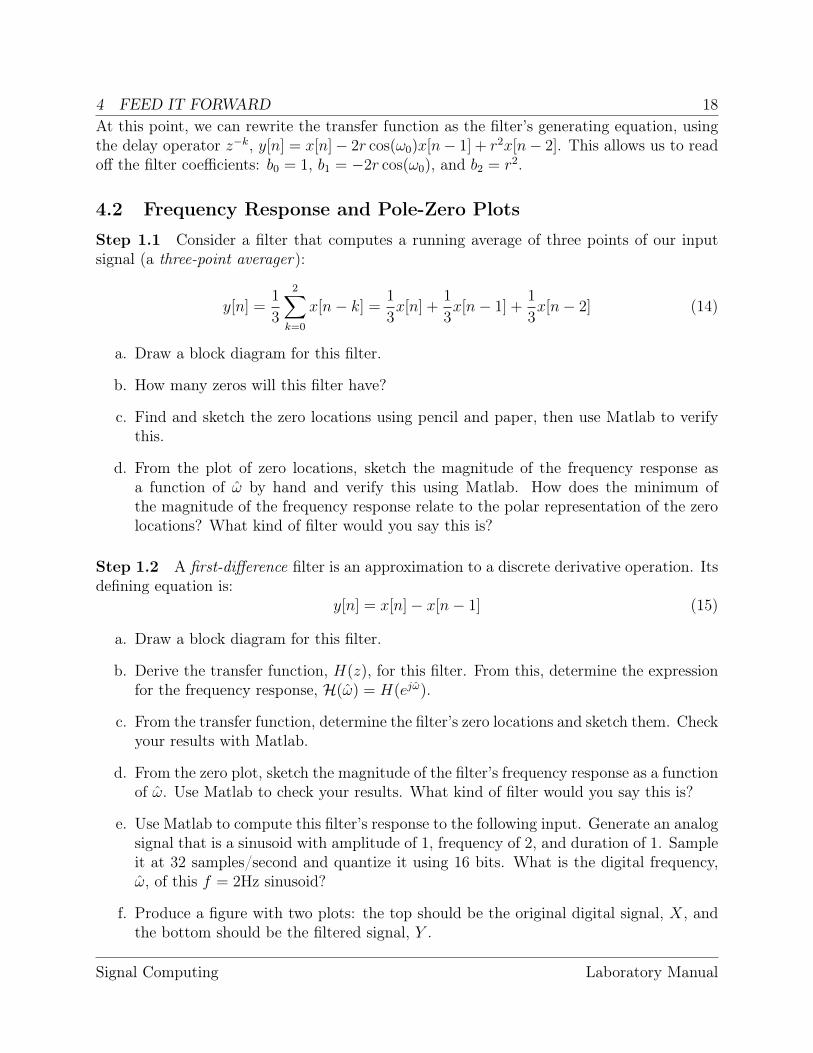
Step 1.1 Consider a filter that computes a running average of three points of our inputsignal (a three-point averager):

y[n] =1

3

2X

k=0

x[n� k] =1

3

x[n] +1

3

x[n� 1] +

1

3

x[n� 2] (14)

a. Draw a block diagram for this filter.

b. How many zeros will this filter have?

c. Find and sketch the zero locations using pencil and paper, then use Matlab to verifythis.

d. From the plot of zero locations, sketch the magnitude of the frequency response asa function of !̂ by hand and verify this using Matlab. How does the minimum ofthe magnitude of the frequency response relate to the polar representation of the zerolocations? What kind of filter would you say this is?

Step 1.2 A first-difference filter is an approximation to a discrete derivative operation. Itsdefining equation is:

y[n] = x[n]� x[n� 1] (15)

a. Draw a block diagram for this filter.

b. Derive the transfer function, H(z), for this filter. From this, determine the expressionfor the frequency response, H(!̂) = H(ej!̂).

c. From the transfer function, determine the filter’s zero locations and sketch them. Checkyour results with Matlab.

d. From the zero plot, sketch the magnitude of the filter’s frequency response as a functionof !̂. Use Matlab to check your results. What kind of filter would you say this is?

e. Use Matlab to compute this filter’s response to the following input. Generate an analogsignal that is a sinusoid with amplitude of 1, frequency of 2, and duration of 1. Sampleit at 32 samples/second and quantize it using 16 bits. What is the digital frequency,!̂, of this f = 2Hz sinusoid?

f. Produce a figure with two plots: the top should be the original digital signal, X, andthe bottom should be the filtered signal, Y .


4 FEED IT FORWARD 19g. Examine the plots of X and Y . Note that Y appears to be a scaled and shifted sinusoid

of the same frequency as X. The exception is the first point, y[0]. Explain why y[0] isdifferent (if you are unsure, consider the defining equation and the input values to itfor n = 0).

h. Estimate the frequency, amplitude, and phase of Y directly from its plot (ignoringy[0]).

i. To compare these measurements to theory, use your expression for the filter’s fre-quency response to calculate the amplitude and phase at the digital frequency !̂ youdetermined above. How do these compare to what you determined from the Matlabplots?

Step 1.3 Just as we can compute a discrete first derivative with a first-difference filter, wecan compute a discrete second derivative with a second difference filter.

a. Use your expression for the transfer function of the first difference filter and yourknowledge that the combined transfer function of two filters cascaded, or connected inseries, is the product of their individual transfer functions to determine the transferfunction for a second-difference filter.

b. Draw a block diagram for this filter.

c. Determine the filter’s zero locations and sketch them. Check your results using Matlab.

d. From the zero plot, sketch the magnitude of the filter’s frequency response as a functionof !̂. Use Matlab to check your results. What kind of filter would you say this is?

Step 1.4 Consider a feedforward filter with complex conjugate zeros at z1,2 = �0.5± j0.5.

a. Determine the filter coefficients.

b. Use Matlab to plot the frequency response of the filter.

c. What are the effects of the zeros on the frequency response? What kind of filter wouldyou call this?

4.3 Linearity and Cascading Filters

Step 2.1 A system is called linear if a sum of different inputs produces an output that isthe sum of the outputs for the inputs taken individually. Perform a simple test of the linearityof the filter from step 1.2 by doubling the input amplitude in Matlab (X 0

= 2X = X +X).How does the new output amplitude compare to the old one?


4 FEED IT FORWARD 20Step 2.2 In one of the self-test exercises in the textbook, two filters with transfer functionsH1(z) = b0 + b1z�1 and H2(z) = b00 + b01z

�1 were connected in series, and it was shown thatthey could be connected in either order to produce the same composite effect (the sameoverall transfer function). Redo this exercise using the defining equations for the two filters,i.e., y1[n] = F1(x[n]) for the filter with transfer function H1(z) and y2[n] = F2(x[n]) for thefilter with transfer function H2(z). In other words, show that F2(F1(x[n])) = F1(F2(x[n])).

Step 2.3 Use Matlab to implement a 50% duty cycle square wave with amplitude 1,frequency 2Hz, and duration 1s. Sample and quantize it appropriately (to make your figureslook nicer, feel free to chose a sampling rate much higher than the minimum). Send theresultant digital signal through the previously-defined three-point averager filter, and thenthe output of that filter through the first difference filter. Plot the input and output. Whatdoes the output of this combined filter look like?

Step 2.4 Now, switch the order you apply the filters so that the first difference filter is firstand the three-point averager is second. Plot the input and output. How does the outputof this configuration compare to that of the preceding step? Does this match what youexpected? Why or why not?


5 LET’S CATCH SOME Z’S 215 Let’s Catch Some Z’s

This lab covers the z-transform, used to convert arbitrary digital signals to the frequencydomain. It also exercises the relationship between a filter’s transfer function and impulseresponse and how the operations of multiplication and convolution, respectively, can be usedto compute a filter’s output.

5.1 The z-transform, Transfer Function, & Impulse Response

A discrete signal x[n] has a z-transform X(z) defined by the following equation:

X(z) =1X

n=0

x[n]z�n

With this definition lets investigate a feed forward filter with ten coefficients, {b0, b1, · · · , b9}.Recall that the Matlab filter function allows us to specify a filter in terms of its coefficients,but we can also think of it as being defined in terms of its transfer function. Considering thebk coefficients of the above feed forward filter, the filter function implements the transferfunction:

H(z) =9X

k=0

bkz�k (16)

In previous labs we have computed the transfer function using the delays of the definingfunction. Mathematically, we were actually taking the z-transform of the impulse response!In this example, the impulse response is:

h[n] =9X

k=0

bk�[n� k] (17)

where �[k] is the unit impulse and only has a non-zero value at k = n. H(z) and h[n] forma z-transform pair, h[n] z ! H(z). It should now be obvious why feedforward filters are alsoknown as finite impulse response filters — their impulse response only has a finite numberof values. To compute the output, y[n], using the impulse response we use convolution.Namely, we convolve the input, x[n], by the impulse response, h[n],

y[n] = x[n] ⇤ h[n] =9X

k=0

x[k]h[n� k] (18)

And, indeed, Matlab has a conv function to do this convolution. Alternatively, we cancompute a filter’s output by multiplying the transfer function by the z-transform of theinput to yield the z-transform of the output:

Y (z) = H(z)X(z) (19)


5 LET’S CATCH SOME Z’S 22From a practical point of view, of course, it makes more sense to implement a filter in termsof its impulse response. However, for filters with long impulse responses, it is sometimesmore convenient to represent them mathematically using the transfer function (which wenow know is just the z-transform of the impulse response!).

5.2 Z-Transforms

Step 1.1 On paper, compute the z-transform, X(z), of

x[n] =

⇢(�1)n n � 0

0 n < 0

(20)

Note that this is an infinite geometric series. What are the locations of any pole(s) (roots ofthe denominator polynomial) or zero(s) (roots of the numerator polynomial)?

Step 1.2 Evaluate the frequency response of X(z) from step 1.1, X(z)��z=ej!̂

, by sketchingit by hand. What kind of filter is this?

Step 1.3 Consider the z-transform:

X(z) = 1� 2z�1+ 3z�3 � z�5 (21)

Write the inverse z-transform, x[n], as a table of values for corresponding n values.

5.3 Impulse Response

Step 2.1 Consider a filter with a transfer function

H(z) = 1 + 5z�1 � 3z�2+ 2.5z�3

+ 4z�8 (22)

What is the defining equation for this filter, y[n] = F (x[n])?

Step 2.2 What is the output sequence of the filter of Step 2.1 when the input is x[n] = �[n]?Verify this using Matlab.

Step 2.3 The impulse response of a filter is h[n] = �[n] + 2�[n � 1] + �[n � 2] � �[n � 3],or equivalently, h[n] = {1, 2, 1,�1}, n = {0, 1, 2, 3}. Determine the response of the systemto the input signal x[n] = {1, 2, 3, 1}, n = {0, 1, 2, 3} by hand. Use Matlab to check yourresults. Include a figure that shows both the input and output signals; make sure the readercan clearly see what the signal values are (the stem plot function should help to ensure thisis the case).

Step 2.4 Change the input to the filter of Step 2.3 to be �[n]. What are the output values?How do they compare to the impulse response? Include plots of the filter input and outputvalues in your report.


5 LET’S CATCH SOME Z’S 23Step 2.5 Use Matlab to determine the output of the filter {1/3,1/3,1/3}, n = {0, 1, 2} forthe input:

x[n] = 4 + sin[0.25⇡(n� 1)]� 3 sin[(2⇡/3)n] (23)

Include a listing of your Matlab code and a figure with plots of the filter input and outputin your report. Is the result expected? Why or why not?

Step 2.6 Create your own Matlab function, convolution, to implement a convolutionfunction. To test your function, make sure it works exactly like the Matlab conv and filter

functions by providing the same input to each and subtracting their outputs. Use the filter{1/3, 1/3, 1/3}, n = {0, 1, 2} from step 2.5.

5.4 Canceling Sinusoidal Components

Filters can be designed to cancel sinusoids. Implement a filter in Matlab with the followingimpulse response:

h[n] = �[n]� 2 cos(⇡/4)�[n� 1] + �[n� 2] (24)

Step 3.1 Plot the frequency response for this filter. What are the zero locations?

Step 3.2 Use as an input to this filter the signal x[n] = sin !̂n, using the two frequencies!̂ = ⇡/2 and !̂ = ⇡/4. You will need to choose appropriate analog signals, with convenientfrequencies and durations, and then sample them appropriately so they have the correctdigital frequencies. Make sure to verify that you get the correct digital frequencies and thatplots you make are convenient for the reader (for example, neither too many nor too fewcycles)! Compute the filter in Matlab for each of these two inputs, plotting the input andoutput of each. When do you get cancellation?

Step 3.3 Can you modify the filter coefficients to cancel the other sinusoid? If so, showyour work.


6 TO INFINITY AND RESPONSE! 246 To Infinity and Response!

By the end of this lab you should feel comfortable manipulating and using feedback filtersfor simple problems. You should also be comfortable with the concept of a filter with aninfinite impulse response. All feedback filters have an infinite impulse response and are alsoknown as IIR filters. Feedback filters use the previous outputs of the filter, feeding themback to compute the output for the current sample. The “fed back” outputs are weighted bycoefficients, a`.

6.1 A Note About Matlab Filter Coefficients

Note that the Matlab filter function uses negative values for the a` (feedback) coefficients,from the transfer function. In other words, in the text, a second-order feedback filter’sdefining equation might be:

y[n] = a1y[n� 1] + a2y[n� 2] + b0x[n] (25)y[n]� a1y[n� 1]� a2y[n� 2] = b0x[n] (26)

This yields the transfer function:

Y (z)(1� a1z�1 � a2z

�2) = b0X(z) (27)

Y (z)/X(z) =b0

1� a1z�1 � a2z�2(28)

H(z) =b0

1� a1z�1 � a2z�2(29)

The coefficients used by filter, rather than being the a` from the defining equation (25)are the negative a` from the transfer function (29) — the ratio of two polynomials. In otherwords, to properly compute the above filter in Matlab, you will need to use:a = [1.0 �a1 �a2];b = [b0];y = filter(b, a, x);

Note also that in this example the filter includes the a[0] coefficient (of course, per Mat-lab one-based indices, as a(1)), which we will always leave as 1.0 (it’s the first “1” in thedenominator of the transfer function).

And finally, note that one form of the filter function takes a fourth argument, whichis the initial conditions for the feedback delays (used in computing the output values thathave delay terms which come before the first value in the x vector). These default to all zeroif not specified.

6.2 Feedback Filters as Recurrence Relations

You may notice that the defining equation for a feedback filter is in the form of a recurrencerelation. In fact, we can use a feedback filter to implement a recurrence relation if we set


6 TO INFINITY AND RESPONSE! 25the input to be an impulse, x[n] = C�[n], with amplitude C being the initial value for theiteration. Let’s start out with the Fibonacci sequence, which you’ll remember to be:

F [n] =

⇢1 n < 2

F [n� 1] + F [n� 2] n � 2

(30)

We can rewrite this recurrence relation as:

y[n] = y[n� 1] + y[n� 2] + x[n] (31)

and we will get the Fibonacci sequence if we input an impulse (hence, the appearance ofthe x[n] on the right hand side, which serves only to initialize the filter). In Matlab, thiscan be done trivially by taking a vector of all zeros — let’s call this vector x — and settingits first value only (x(1)) to C. This is also a very good demonstration of the first “I” in theacronym “IIR”: the impulse response of this filter has infinite duration.

Step 1.1 If we set x[n] = �[n] in (31), we should see that the impulse response of this filteris indeed the Fibonacci sequence. Implement this filter in Matlab and verify that its impulseresponse is the Fibonacci sequence. What are the values of the coefficients that you used?

Step 1.2 What is the value for n = 19 (y(20) in Matlab)?

Step 1.3 Is this filter stable?

Step 1.4 Let’s do something similar with the recurrence relation for computing the seriesy[n] = 1/3n in the text (as always, remember that Matlab indices start at 1). Set thecoefficients for a feedback filter to implement equation (5-42) in the text, y[n] = 1/3y[n �1] + x[n]. What are the filter coefficients?

Step 1.5 What are the pole location(s) for this filter?

Step 1.6 Now use Matlab to calculate the impulse repsonse. Set the amplitude of theinput impulse to be 0.99996. Is this filter stable? Is its impulse response consistent with theresult of iterating equation (5-42) in the notes?

6.3 Telephone Touch Tone Dialing

Telephone touch pads generate dual tone multi frequency (DTMF) signals to dial a telephone.When any key is pressed, the tones of the corresponding column and row in the table beloware generated, hence it is a “dual tone” code. As an example, pressing the 5 button generatesthe tones 770Hz and 1336Hz summed together.


6 TO INFINITY AND RESPONSE! 261209Hz 1336Hz 1477Hz

697Hz 1 2 3770Hz 4 5 6852Hz 7 8 9941Hz ⇤ 0 #

The frequencies in the table above were chosen to avoid harmonics. No frequency is amultiple of another, the difference between any two frequencies does not equal any of thefrequencies, and the sum of any two frequencies does not equal any of the frequencies.1 Thismakes it easier to detect exactly which tones are present in the dial signal in the presence ofline distortions.

It is possible to decode such a signal by first using a filter bank composed of sevenbandpass filters, one for each of the frequencies above. When a button is pressed, it willproduce a combination of two tones, and thus, at the decoder end, two of the bandpassfilters will produce significantly higher outputs than the others. A good measure of theoutput levels is the average power at the filter outputs. This is calculated by squaring thefilter outputs and averaging over a short time interval.

Step 2.1 First of all, please write a Matlab DTMFCoder function. This function should takein one argument — a telephone key number — and return a digital waveform containingthe appropriate summed tones. Internally, it should do this by generating AnalogSignals,summing them, and then sampling them at 8kHz and quantizing them at 16 bits. DTMFsignal duration should be 1s. For each of the seven tone frequencies in Hz, what is thecorresponding digital frequency in the range [0, ⇡]?

Step 2.2 In this step, please construct a bandpass filter for the 697Hz tone. Use a feedbackfilter with complex conjugate poles. Locate these complex conjugate poles at the correctlocation for ±697Hz. Use equation (5-38) of section 5.1.4 of the text to set the radius ofthose poles so that the closest other tone frequency, 770Hz, lies outside the passband (inother words, to set the bandwidth so that it is significantly smaller than twice the differencebetween 697Hz and 770Hz). What were your pole locations?

Compute the corresponding filter coefficients. You can verify your filter performance byplotting its frequency response.

Verify that the filter output for DTMFCoder output for keys 1, 2, and 3 are pretty muchidentical, and that all other buttons produce much lower amplitude output. In your report,include a plot of the filter output for one of the buttons 1, 2, or 3 and a plot for one of thebuttons 4, 5, or 6.

Step 2.3 Now we are ready to decide whether a particular frequency is present. Write aMatlab RMS function that takes a vector as input and returns a scalar root mean squaredvalue for it — this function should square each value of the vector, take the mean of those

1More information can be found at: http://en.wikipedia.org/wiki/DTMF


http://en.wikipedia.org/wiki/DTMF

6 TO INFINITY AND RESPONSE! 27squares, and then take the square root of that mean. Determine the RMS filter output fortelephone buttons 1, 2, and 3 and compare them to the other phone buttons. You shouldsee a much higher value for 1, 2, and 3 than the other buttons; additionally, the RMS valuesfor those three buttons should be almost identical. What are the RMS values you get forpressing 1 versus 4?

Step 2.4 Now we will assemble a filter bank. Implement filters in Matlab for each of thesix other DTMF frequencies and verify that they work as expected. Now, write a Matlabfunction DTMFDecoder that takes a single input — a vector (for which you will use theDTMFCoder output). DTMFDecoder should compute the RMS value of the output of each ofthe seven filters in the filter bank. It should output (to the Matlab console) these RMSvalues, and then detect the two highest values. It should use a lookup table or equivalentlogic to decode which button was “pressed,” and output (to the Matlab console) that button.


7 JOE FOURIER WAS NOT A DISCRETE FELLOW 287 Joe Fourier Was Not a Discrete Fellow

7.1 Lab Background

By the end of this lab you should have a firm understanding of how the Discrete FourierTransform (DFT) can be implemented exactly using the Fast Fourier Transform (FFT). Inaddition you should be able to identify common problems using the DFT to analyze signals.You will also be familiar with a new tool, the spectrogram, that uses the DFT as a functionof time.

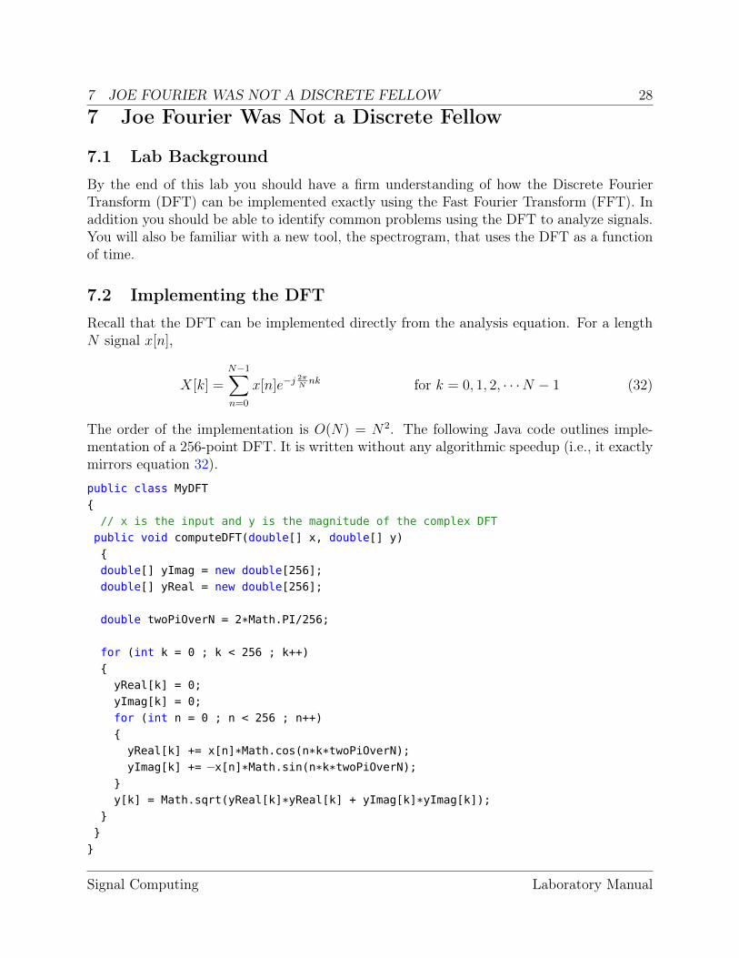
7.2 Implementing the DFT

Recall that the DFT can be implemented directly from the analysis equation. For a lengthN signal x[n],

X[k] =N�1X

n=0

x[n]e�j 2⇡N nk for k = 0, 1, 2, · · ·N � 1 (32)

The order of the implementation is O(N) = N2. The following Java code outlines imple-mentation of a 256-point DFT. It is written without any algorithmic speedup (i.e., it exactlymirrors equation 32).public class MyDFT{// x is the input and y is the magnitude of the complex DFTpublic void computeDFT(double[] x, double[] y){double[] yImag = new double[256];double[] yReal = new double[256];

double twoPiOverN = 2*Math.PI/256;

for (int k = 0 ; k < 256 ; k++){yReal[k] = 0;yImag[k] = 0;for (int n = 0 ; n < 256 ; n++){yReal[k] += x[n]*Math.cos(n*k*twoPiOverN);yImag[k] += �x[n]*Math.sin(n*k*twoPiOverN);

}y[k] = Math.sqrt(yReal[k]*yReal[k] + yImag[k]*yImag[k]);

}}}


7 JOE FOURIER WAS NOT A DISCRETE FELLOW 29Note that, unlike in Matlab, there is no native support in Java for complex numbers

so this arithmetic is written out explicitly in the code above. For example, the equationy = x⇥ ea (where x is a real number) must be explicitly written out using Euler’s formula,and the real and imaginary portions saved in separate variables, yreal = x ⇥ cos(a) andyimag = x⇥ sin(a).

The FFT algorithm can be used to reduce the computation time of the DFT to O(N) =

N log2 N — a significant speedup for even modest length signals.

7.3 The FFT in Matlab

Matlab includes a fft function (there are many more related operations in the Signal Pro-cessing Toolbox, but we are sticking to “vanilla” Matlab here). You can look at the docu-mentation for this function; pay especial attention to the frequency values that correspondto each element of the vector that this function returns, and to how to specify the numberof points in the FFT it computes.

Step 1.1 Implement your own myFFT function in Matlab that takes a real-valued vector asinput, computes a 256-point FFT, and returns a real-valued vector that is the magnitude ofthe (single-sided, i.e., only positive frequencies) FFT. Implement this function using loops(i.e., do not use recursion). The first part of this code performs a bit reversal on the inputarray. You can use the following code to perform the bit reversal efficiently (efficient bitreversal algorithms in other languages are typically more complex):% Assume that you want to do a bit reversal of the contents of the vector xindices = [0 : length(x)�1]; % binary indices need to start at zerorevIndices = bin2dec(fliplr(dec2bin(indices, 8))); % bit reversed indicesrevX = x(revIndices+1); % Add 1 to get Matlab indices

This code converts the vector of in-order indices to an array of 8-character strings (repre-senting those indices as binary 8-bit numbers). Each string is then reversed, and convertedback to numbers. The resultant vector of indices (which is what they are after we add oneto each) is applied to the signal to pull its entries out into a new vector, with the order ofthe entries in bit-reversed order.

Once you’ve done this, all you need to do is iterate over the array log2 N times! Rememberthat you’re performing complex arithmetic and to compute the magnitude of the output arrayonce the FFT is computed. Include a copy of your Matlab code in your report.

Step 1.2 Check your results using the Matlab fft function. Your results should be quitesimilar, if not identical; this should be apparent by comparing graphs of the outputs. Take theFFT of a sinusoid with a frequency of ⇡/4 radians per second using your FFT implementationand the fft function.

Step 1.3 Prove that the number of complex multiplies performed by your code is O(N logN).


7 JOE FOURIER WAS NOT A DISCRETE FELLOW 307.4 Using the DFT

Step 2.1 Create a sum of two sinusoids. Use the built-in Matlab fft function (it will allowyou, among other things, to apply an n-point FFT to a signal with more than n samples) tocompute the FFT of the sum and then plot the FFT magnitude. Use frequencies of 0.13⇡and 0.19⇡ for the two sinusoids. Make sure that there are at least 256 samples in eachwaveform, as you’ll want to use a 256-point FFT! Also, make sure you correctly computethe corresponding frequency values (either from 0 to ⇡ or �⇡ to ⇡, depending on whetheryou prefer plotting the single-sided magnitudes or not) for the FFT X-axis, and label itappropriate in your graph. What does the result look like? Does this make sense?

Step 2.2 At what index (or indices) does the FFT magnitude reach its peak value(s)?What frequency (or frequencies) does this correspond to?

Step 2.3 Change the frequencies of the sinusoids to 0.13⇡ and 0.14⇡. Repeat steps 2.1and 2.2. Do the results still make sense?

Step 2.4 Replace the sum of two sinusoids with your DTMFCoder function from lab 6.Input a selection of button values. Does the FFT block show the separate frequencies foreach button?

7.5 Spectrograms

Comparing FFT graphs (as in the step 2.4 above) can be difficult to do. But what if wecould analyze the frequency content of a signal as a function of time? That would make iteasier to see differences in frequency if a signal started changing (like a string of DTMF keyspressed in turn). To do this we will need a new tool called the Spectrogram. The spectrogramis simply an algorithm for computing the FFT of a signal at different times and plottingthem as a function of time. The spectrogram is computed in the following way:

1. A given signal is “windowed.” This means that we only take a certain number of pointsfrom the signal (for this example assume we are using a window of length 128 points).To start out, we take the first 128 points of the signal (points 1 through 128 of theinput vector).

2. Take the FFT of the window and save the it in a separate array.

3. Advance the window in time by a certain number of points. For instance we canadvance the window by 64 points so that we now have a window of indices 65 through192 from the input signal array.

4. Repeat steps 1–3, saving the FFT of each window, until there are no longer any pointsin the input array.


7 JOE FOURIER WAS NOT A DISCRETE FELLOW 315. Form a 2-D matrix whose columns are the FFT magnitudes of each window (placed

in chronological order). In this way, each row represents a certain frequency, eachcolumn represents a given instant in time, and the value of the matrix represents themagnitude of the FFT.

The result is called a spectrogram and is usually displayed as an RGB image whereblue represents small FFT magnitudes and red represents larger FFT magnitudes (the Jetcolormap if you are familiar with color visualizations). There is an art to choosing the correctparameters of the spectrogram (i.e., window size, FFT size, how many points to advancethe FFT, etc.). Each parameter has tradeoffs for the time and frequency resolution of theresulting spectrogram. For our purposes here, we will not be concerned with these tradeoffs.Instead we will be more interested in getting familiar with analysis using spectrograms.

The Matlab Signal Processing Toolbox has a spectrogram function, but you can re-trieve a drop-in replacement for it from http://www.ee.columbia.edu/ln/rosa/matlab/

sgram/ that will work without that toolbox. See the online Matlab documentation for thespectrogram function to understand what the parameters to that function are (though, forour purposes, you should just be able to use the call y = myspecgram(x).

Step 3.1 Use your DTMFCoder function again. Instead of computing its FFT, computeits spectrogram instead. What does the spectrogram look like for button 1? Are bothfrequencies present?

Step 3.2 For this step, use DTMFCoder to generate the codes for multiple buttons — atleast three — and concatenate them together to form a single vector. Does the spectrogrammake it easier to judge the frequency content of the keys? Can you clearly see when thesignal changes from one key to another?


http://www.ee.columbia.edu/ln/rosa/matlab/sgram/

http://www.ee.columbia.edu/ln/rosa/matlab/sgram/

8 I’M SO COMPRESSED 328 I’m So Compressed

8.1 Sound and images in MATLAB

MATLAB has a number of functions that can be used to read and write sound and imagefiles as well as manipulate and display them. See the help for each function for details. Onesthat you’ll likely find useful are:

audiorecorder Perform real-time audio capture. This may or may not work on your system;it is critically dependent on your hardware and MATLAB’s support thereof. You mayfind it simpler to record and edit audio files with other software and then save it to afile later read into Matlab; this might give you greater control over the recording.

audioinfo Get information about an audio file, including number of channels, how com-pressed, sampling rate, bits per sample, etc.

audioread Read part or all of an audio file, returning sampled data and sampling rate.

audiowrite Write an audio file; the format is indicated by the filename provided. Allplatforms support wav, .ogg, and .flac; Windows and OS X support .m4a and .mp4,too.

sound Play vector as a sound. This allows you to create arbitrary waveforms mathemati-cally (e.g., individual sinusoids, sums of sinusoids) and then play them through yourspeakers. This is the function to use if you’re values are scaled within the range of -1to +1.

soundsc This function works like sound, but first it scales the vector values to fall withinthe range of -1 to +1. Much of the time, you won’t have your waveforms pre-scaled,and you’ll use this function.

imfinfo Provides information about an image file, including dimensions, bit depth, etc.

imread Read image from graphics file. This function (and imwrite) supports many filetypes.

imwrite Write image to graphics file.

image Display image. The image is displayed within normal Matlab axes, which you canlabel or otherwise modify as usual. Any 2D array can be displayed as an image (forexample, this is what’s done with the output of myspecgram). You can alter thecolormap used for this display, if you like. There are other functions that plot 2D dataas wire meshes and surfaces.

imagesc Like image, but scales the image values first so that they span the full range ofthe current colormap.


8 I’M SO COMPRESSED 33There are a number of other functions available; read the Matlab documentation to get thefull scoop on what is available and how it works.

Within MATLAB, audio is a 1-D vector (stereo is n⇥ 2, but we won’t deal with stereo)and gray-scale images are 2D arrays (color images are 3-D arrays). For simplicity’s sake,make sure any sound files you use are mono.

8.1.1 Data Types

MATLAB supports a number of data types, and the type that the file I/O functions returnoften depends on the kind of file read. Regardless, almost all of the MATLAB functionsyou’ll use to process data return doubles. For example, consider the following commandsthat read a color image, convert it to gray-scale, and display it:>> A = imread('/tmp/ariel.jpg');>> B = mean(A,3);>> imagesc(B)>> colormap(gray)>> axis equal>> whosName Size Bytes Class

A 100x55x3 16500 uint8 arrayB 100x55 44000 double array

The (color) image is read into A, which, as you can see from the output of the whos command,is a 100x55x3 unsigned, 8-bit integer array (the third dimension for the red, green, and blueimage color components). I convert the image to gray-scale by taking the mean of thethree colors at each pixel (the overall brightness), producing a B array that is double. Theimagesc function displays the image, the colormap function determines how the array valuestranslate into screen colors, and the axis equal command ensures that the pixels will besquare on the screen.

Much of the time, we will just perform our calculations using double data types. However,we can use functions like uint8 to convert our data.

At the very least, you can get real audio files from http://faculty.washington.edu/

stiber/pubs/Signal-Computing/; I assume that you’ll have no trouble locating interestingimages (please keep your work G-rated). Don’t use ones that are too big, to avoid issueswith Canvas uploads of large lab report files.

8.2 Lossless image coding

The simplest way to compress images is run-length coding (RLE), a form of repetitivesequence compression in which multiple pixels with the same values are converted intoa count and a value. To implement this, we need to reserve a special image value —one that will never be used as a pixel value — as a flag to indicate that the next twonumbers are a (count, value) pair, rather than just a couple pixels. Let’s apply RLE to




8 I’M SO COMPRESSED 34three different kinds of images: color photographs, color drawings, and black-and-white im-ages (e.g., a scan of text). You can choose images you like, or get these from the bookweb site: http://faculty.washington.edu/stiber/pubs/Signal-Computing/ariel.jpg(color photo), http://faculty.washington.edu/stiber/pubs/Signal-Computing/cartoon.png (color drawing), and http://faculty.washington.edu/stiber/pubs/Signal-Computing/

text.png (black-and-white).

Step 1.1 Write a MATLAB script to read an image in, convert it to gray-scale if the imagearray is 3-D, and scale the image values so they are in the range [1, 255] (note the absence ofzero). Verify that this has worked by using the min and max functions. Convert the resultsto uint8 and display each using imagesc.

Step 1.2 At this point, you should have in each case a 2-D array with values in the range[1, 255] inclusive. To simplify matters, we will treat each array as though it were one-dimensional. This is easy in MATLAB, as we can index a 2-D array with a single indexranging from 1 to N ⇥M (the array size). Write a RLE function that takes in a 2-D arrayand scans it for runs of pixels with the same value, producing a RLE vector on its output.When fewer than four pixels in a row have the same value, they should just appear in thevector. When four or more (up to 255) pixels in a row have the same value, they should bereplaced with three vector elements: a zero (indicating that the next two elements are a runcode, rather than ordinary pixel values), a count (should contain 4 to 255), and the pixelvalue for the run. Verify that your RLE function works by implementing a RLD function(RLE decoder) that takes in a RLE vector, N , and M and outputs a 2-D N ⇥M array.The RLD output should be identical to the RLE input (subtracting them should produce anarray of zeros); verify that this is the case. For each image type, compute the compressionfactor by dividing the number of elements in the RLE vector by the number of elements inthe original array. What compression factors do you get for each image?

8.3 Lossy audio coding: DPCM

In differential pulse-code modulation (DPCM), we encode the differences between signalsamples in a limited number of bits. In this section, you’ll take an audio signal, applyDPCM with differing numbers of bits, see how much space is saved, and hear if and how thesound is modified. A slight complicating factor is that all of the data will be representedusing double, however, we will limit the values that are stored in each double to integers inthe range [0, 2bits � 1] (where “bits” is the number of bits we’re using).

Step 2.1 Find a sound to work with; you can use http://faculty.washington.edu/

stiber/pubs/Signal-Computing/amoriole2.mat if you like. Likely, it will have valuesthat are not integers; convert the values to 16-bit integer values by scaling (to [0, 216 � 1])and rounding (reminder: the vector’s type will still be double; we’re just changing the values


http://faculty.washington.edu/stiber/pubs/Signal-Computing/ariel.jpg

http://faculty.washington.edu/stiber/pubs/Signal-Computing/cartoon.png

http://faculty.washington.edu/stiber/pubs/Signal-Computing/cartoon.png

http://faculty.washington.edu/stiber/pubs/Signal-Computing/text.png

http://faculty.washington.edu/stiber/pubs/Signal-Computing/text.png

http://faculty.washington.edu/stiber/pubs/Signal-Computing/amoriole2.mat

http://faculty.washington.edu/stiber/pubs/Signal-Computing/amoriole2.mat

8 I’M SO COMPRESSED 35in each element to be integers in that range). Verify that this conversion produces no audiblechange in the sound. What is the MATLAB code to do this initial quantization?

Step 2.2 Now write a DPCM function, DPCM, that takes the sound vector and the numberof bits for each difference and outputs a DPCM-coded vector. Note that the MATLAB diff

function will compute the differences between sequential elements of a vector. Your DPCMfunction should:

1. compute the differences between the samples,

2. limit each difference value to be in the range [�2bits�1 � 1, 2bits�1 � 1], producinga quantized vector and a vector of “residues” (you will generate two vectors). Foreach quantized difference, the “residues” vector will be zero if the difference, �xi, iswithin the above range. Otherwise, it will contain the amount that �xi exceeds thatrange (i.e., the difference between �xi and its quantized value, either �2bits�1 � 1 or2

bits�1 � 1).

3. “make up for” each nonzero value in the “residues” vector. For each such value, scanthe quantized difference vector from that index onward, and modify its entries, up tothe quantization limits above, until all of the residue has been “used up”.

4. The final result is a single coded vector that your function should return.

For example, let’s say that we’re using 4 bit DPCM and that some sequence of differencesis (�x1 = 10,�x2 = 5,�x3 = �3). The range of quantized differences is [�7,+7], and sothe quantized differences are (7, 5,�3) and the residues are (3, 0, 0). Since the first residueis nonzero, we proceed to modify quantized differences starting with the second one, untilwe’ve added three to them. The resulting final quantized differences are (7, 7,�2).

Step 2.3 Implement an inverse DPCM function IDPCM that takes the first value from theoriginal sound vector and the DPCM vector and returns a decoded sound vector. There’sno way for us to know where the losses in the encoding occurred, so we just use the DPCMvalues as differences. Note that the MATLAB cumsum function computes a vector withelements being the cumulative sum of the elements of its input vector, and that you can adda constant to all of the elements of a vector using the normal addition operator.

Step 2.4 Test your DPCM and IDPCM functions by coding your sound using 15, 14, 12,and 10 bit differences. At what point does the coding process produce noticeable degrada-tion? To investigate further, see how few bits you can use to encode the sound and stilldetect some aspect of the original sound. Is this surprising to you?


8 I’M SO COMPRESSED 368.4 Lossy image coding: JPEG

Step 3.1 In this sequence of steps, we will use frequency-dependent quantization, similarto that used in JPEG, to compress an image. Start with your gray-scale, continuous-toneimage from step 1.1 (if you used a color image, convert it to gray-scale as you did in step 1.1).The MATLAB image processing or signal processing toolboxes are needed to have access toDCT functions, so we’ll use the fft2() and ifft2() functions instead. To do a basic test ofthese functions, write a script that loads your image, converting it to gray-scale if necessary,and then computes its 2D FFT using fft2(). The resulting matrix has complex values,which we will need to preserve. Display the magnitude of the FFT (remember to use theabs function to get the magnitude of a complex number) using imagesc(). Do this for eachimage type. Can you relate any features in the FFT to characteristics in the original image?

Step 3.2 Use ifft2() to convert the FFT back and plot the result versus the originalgray-scale image (use imagesc()) to check that everything is working fine. Analyze thedifference between the two images (i.e., actually subtract them) to satisfy yourself that anychanges are merely small errors attributable to finite machine precision). Repeat this processfor the other images.

Step 3.3 Let’s quantize the image’s spectral content. First, find the number of zero ele-ments in the FFT, using something like origZero=length(find(abs(a)==0));, where a isthe FFT. Remember to exclude the DC value in the fft2 output in figuring out this range.Then, zero out additional frequency components by zeroing out all with magnitudes belowsome threshold. You’ll want to set the threshold somewhere between the min and max mag-nitudes of a, which you can get as mn=min(min(abs(a))); and mx=max(max(abs(a)));.Let’s make four tests, with thresholds 5%, 10%, 20%, and 50% of the way between the minand max, i.e., th=0.05*(mx-mn)+mn;. Zero out all FFT values below the threshold usingsomething like:b = a;b(abs(a)<th) = 0; % Uses logical array indexing

You can count the number of elements thresholded by finding the number of zero elements inb at this point and subtracting the number that were originally zero (i.e., origZero). Thisis an estimate of the amount the image could be compressed with an entropy coder. Expressthe number of thresholded elements as a fraction of the total number of pixels in the originalimage and make a table or plot of this value versus threshold level.

Optional. Note that the FFT may have very high values for just a few elements, and lowvalues for others. You might plot a histogram to verify this. Not including the DC valuelikely will eliminate the highest value in the FFT. However, some of the other values maystill be large enough to produce too large of a range. Can you suggest an approach that willtake this into account? How does the JPEG algorithm deal with or avoid this problem?


8 I’M SO COMPRESSED 37Step 3.4 Now we will see the effect of this thresholding on image quality. Convert thethresholded FFT back to an image using something like c = abs(ifft2(b));. For eachtype of image and each threshold value, plot the original image and the final processedimage. Compute the mean squared error (MSE) between the original and reconstructedimage (mean squared error for matrices can be computed as mean(mean((a-c).^2))). Whatcan you say about the effects on the image and MSE? Collect your code together as a scriptto automate the thresholding and reconstruction, so you can easily compute MSE for anumber of thresholds. Plot MSE vs. threshold percentage (just as you plotted fraction ofpixels thresholded vs. threshold in step 3.3).


Documents

Signal Computing: Digital Signals in the Software Domain