Shunting operations at flat yards: Retrievingfreight railcars from storage tracks

WORKING PAPERMay 2016

Florian JaehnSustainable Operations and Logistics, University of Augsburg, Germany

florian.jaehn@wiwi.uni-augsburg.deAlena Otto

Management Information Science, University of Siegen, Germanyalena.otto@uni-siegen.de

Kilian SeifriedLogistics and Supply Chain Management, University of Mannheim, Germany

kilian.seifried@bwl.uni-mannheim.de

Abstract

In this paper, we study the railcar retrieval problem (RRT) where speci-fied numbers of certain types of railcars have to be withdrawn from the stor-age tracks of a flat yard. This task arises in the daily operations of workshopyards for railcar maintenance. The objective is to minimize the total cost ofshunting via methods such as minimizing the usage of shunting engines.

We describe the RRT formally, present a mixed-integer program formu-lation, and prove the general case to be NP-hard. For some special cases,exact algorithms with polynomial runtimes are proposed. We also analyzeseveral intuitive heuristic solution approaches motivated by observed real-world planning routines. We evaluate their average performances in sim-ulations with different scenarios and provide their worst-case performanceguarantee. We show that although the analyzed heuristics result in muchbetter solutions than the naive planning approach, they are still on average30%-50% from the optimal objective value and may result in up to 14 timeshigher costs in the worst case. Therefore, we conclude that optimizationshould be implemented in practice in order to save valuable resources. Fur-thermore, we analyze the impacts of yard layout and the widespread organi-zational routine of presorting on the railcar retrieval cost.

1 IntroductionOne of the current priorities in transport policy is the promotion of freight railtransportation to reduce carbon dioxide emissions and to relieve congested roads[7]. However, rail companies still have to reduce the costs and travel times ofcustomer freight to increase the attractiveness of rail transportation. One of theimportant cost drivers is railcar maintenance. Annual railcar operation, routinemaintenance and repair costs amount to about $800 and $10,000 per railcar de-pending on its type, age and annual mileage [4]. Recently, maintenance has re-ceived high visibility due to the large-scale modernization of freight railcars withmodern K- and LL-blocks, so-called low-noise blocks made of more protectivematerials that reduce the wearing-off of railcar wheels, as a part of the Europeannoise-reduction program.

Railcar maintenance is not a trivial task for companies: it takes a lot of timeand resources. A railcar in operation visits a repair shop several times a year, andapproximately two of these visits are unplanned [12]. For relatively new (three-to seven-year-old) intermodal double pocket railcars, the time to recovery usuallylasts more than 10 days, and in 20% of cases, it even exceeds 40 days [18]. Thesenumbers are even higher for a typical railcar in Germany because the averagefreight railcar age is approximately 21–30 years [21].

Railcars spend significant portions of their downtimes associated with main-tenance and repair on storage tracks awaiting the opening of a suitable workshoplane and the arrival of ordered parts at the workshop. If the waiting time is ratherlong, railcars are put on storage tracks at low-cost sites, which are as a rule farfrom the workshops. The storage tracks in Hamm/Germany, for example, mainlyhost railcars from the workshop in Paderborn/Germany. Periodically, usually oncea day, railcars of certain types ordered by the workshop are retrieved from the stor-age tracks, assembled into a train and delivered to the workshop. Because storagetracks represent a flat yard with no hump or hill that facilitate shunting, the re-trieval of railcars is a very time consuming and expensive operation. Moreover,due to the variability inherent in maintenance and repair, the planning time hori-zon of the repair workshops is rather short. Therefore, faster retrieval will increasethe utilization of the workshop resources and speed up the time to recovery of therailcars.

In this paper, we are looking for the most efficient policies for the retrievalof railcars of given types from storage tracks. In other words, for the specifiedparking positions and types of railcars on the storage tracks, we decide whichrailcars have to be withdrawn so that the shunting cost and time are minimized.

Considering the large amount of academic literature already published onshunting operations, see Hansmann and Zimmermann [11], Gatto et al [9] andBoysen et al [2] for surveys and literature reviews, there is astonishingly little

2

research that might assist practitioners in the outlined planning problem. The ma-jority of the literature deals with the re-ordering of railcars according to a specifiedsequence. The objective is usually to minimize the number of classification tracksor the number of classification stages. In contrast, we investigate the retrieval of alimited number of railcars of certain types, thereby the sequence of the retrievedrailcars can be arbitrary.

Another core theme in the shunting literature is devoted to operations in depotsof self-propelled vehicles, as a rule passenger train units or trams (see, e.g., DiStefano and Koci [5], Winter and Zimmermann [22], and Blasum et al [1]). Acommon objective here is to position the arriving vehicles on storage tracks sothat they do not block each other while departing from the depot. This problemsetting is different from ours because when the railcars arrive, we do not knowwhen they will be transported to the workshop or which railcars will be a part ofthe same request.

The work that comes closest to the problem in our paper is conducted byLübbecke and Zimmermann [17]. The authors analyze the allocation of railcarswithin in-plant rail networks, specifically which yards have to supply railcars ofthe required types to the points of demand so that transportation and shunting costsare minimized. Two sub-problems arise: how many railcars of each type will besupplied from each yard for each request, and how to retrieve the railcars of therequested types from a given yard. The latter problem is similar to ours, except forthe assumption that the railcar retrieval cost depends linearly on the order numberof the railcars on the track. In other words, it is about three times more expensiveto retrieve the ninth railcar on the track than the third railcar. This assumptiondoes not hold in our problem, where the engine can dislocate a block of railcars inone move (see Section 2).

To the best of our knowledge, only Hall [10] examines operations at railcarmaintenance centers. He performs strategic layout analysis, and as a part of theanalysis, Hall [10] develops analytical formulas on the expected number of shunt-ing moves under some restrictive assumptions (e.g., retrieval of only one railcar ata time, random distribution of railcars on tracks and a retrieval cost that is linearwith the order number of the railcar).

Several articles investigate operations at rail maintenance centers in general,without taking railcars or storage tracks into account explicitly [19, 20, 13]. Theydevelop models for scheduling operations to critical resources of limited capac-ities. These articles do not treat shunting as a part of optimization, instead theyassume certain retrieval policies, such as FIFO or LIFO.

Note that we are not dealing with a general problem of scheduling mainte-nance and repair operations in this paper. We refer the interested reader to, e.g.,Doganay and Bohlin [6] and Budai et al [3] and to the general reviews of Kobbacyand Murthy [15] and Lidén [16].

3

Figure 1: Example of K = 20 railcars of types t = 0, 1, 2, 3 on storage tracks. The dotted linevisualizes the movement of the engine transporting railcars 3 and 4 to the collecting track α

In the following, we set up the problem and analyze its complexity in Sec-tions 2 and 3, respectively. In Section 4, we provide the performance guaranteefor several heuristic solution approaches, motivated by the planning routines ob-served in practice. We proceed with extensive computational experiments andmanagerial insights in Section 5. We conclude with final remarks and an outlookin Section 6.

2 The railcar retrieval problemWe can summarize the railcar retrieval problem (RRT) as follows. Given railcarsof different types (marked with different colors in the example in Figure 1) parkedon storage tracks, we have to retrieve the specified number of railcars of certaintypes in a way such that the retrieval cost is minimized.

In the following (Section 2.1), we describe the practical motivation of theRRT first in order to understand the underlying assumptions. Afterwards, in Sec-tion 2.2, we state the RRT formally.

2.1 Practical motivation for the RRTThe length and the number of storage tracks highly depend on the size of theallotment. Often these are about 800–900 meter long tracks. Although sometracks are accessible from both sides, only one of them, which we call the headof the track (cf. Lübbecke and Zimmermann [17]), is used for the retrieval ofrailcars.

The workshop order specifies how many railcars of certain railcar types arerequested. As a rule for each type t, there are many more railcars stored on thetracks than requested in the order. Indeed, although dozens of railcar categoriesexist (such as refrigerator boxcars, flat logging railcars, and intermodal doublepocket railcars), about 90% of railcars belong to only a handful (about five) cate-gories. Moreover, the railcars in each category often require the same kind of re-

4

pair or maintenance. The most widespread repairs include the wheels of all kindsof railcars, the carriage bodies of gondolas transporting scrap that often becomedeformed, the valves of tank railcars, etc.

The railcars are retrieved by a shunting engine and assembled on a specialtrack α into a train (see Figure 1). Let us look at a retrieval operation that involvesmoving railcars 3 (type 2) and 4 (type 1) to track α (the movements of the engineare depicted with gray dotted arrows in Figure 1). First, the engine picks uprailcars 1, 2, 3 and 4 and moves them to the intermediate position β. After amember of the shunting team has switched the track, the engine transports therailcars backwards to the collecting track α. Then, railcars 3 and 4 are decoupled,and the engine returns to position β with the rest of the railcars. Afterwards,the switches are repositioned, the engine pushes railcars 1 and 2 to their track,railcars 1 and 2 are coupled to the rest of the railcars, and if needed, they aredecoupled from the shunting engine. Now, the shunting engine is ready for thenext retrieval operation. This kind of yard in which no hill or hump assists theshunting process is called a flat yard. As one can see, shunting in a flat yardis a very time consuming process because of the many manual steps (switching,sometimes coupling and decoupling of the railcars), the stop-and-go operation ofthe engine, the low speed limits and the long distances for shunting unit workers.It takes several hours to assemble a train of 20–40 railcars, which is the typicalsize of a workshop order.

If we retrieve several consecutive railcars together as a block, we incur aboutthe same cost as for the retrieval of a single railcar. In our example, the sameengine moves, the same switching and similar further supporting procedures willbe incurred if we would retrieve railcar 3 alone versus railcar 3 together withrailcar 4. Moreover, the operation of the critical resource, the engine, is usuallythe bottleneck and determines the duration of the retrieval.

The retrieval cost is lower if we can retrieve a block of railcars whose firstrailcar is positioned at the head of the track. Indeed, we can attach this block tothe outgoing train in the last step, so that the shunting engine does not need tovisit collecting track α.

The sequence of the retrieved railcars can be arbitrary because they are clas-sified upon arrival at the maintenance center. The railcars are assigned to freeworkshop lanes or to on-site storage tracks for short waiting times.

Our aim is to retrieve as few blocks of consecutive railcars as possible. Specif-ically, we aim at minimizing the total time of retrieval operations. Another possi-ble objective is to reduce the operation costs of the critical resource, which is theshunting engine.

5

2.2 Formal description of the RRTThe RRT can be described as follows.

Instance: Given the following data

• a set {1, 2, . . . , K} (of railcars),• a set {0, . . . , T}, T < K (of railcar types),• a surjective mapping u : {1, 2, . . . , K} → {0, 1, . . . , T} (defining the

railcars’ types),

• a vector (n1, ..., nT ) ∈ NT with N :=T∑t=1

nt < K (demand vector, or

workshop’s order),• a subset K ′ ⊆ {1, 2, . . . , K} with 1 ∈ K ′ (of first railcars on each

track),• and cost parameters 0 ≤ z0 ≤ z1.

Question: Determine X ⊆ {1, 2, . . . , K} with |{x ∈ X|u(x) = t}| = nt, ∀t ∈{1, . . . , T} and {x ∈ X|u(x) = 0} = ∅ such that the following objective isminimized:

z0 · |{x ∈ X|x ∈ K ′}|+ z1 · |{x ∈ X|x /∈ K ′, x− 1 /∈ X}|

Here, the K railcars are positioned on parallel storage tracks such that the railcarnumbers are increasing on each track. The first railcar on each track is defined byset K ′. For each railcar, its type is defined by the function u. We may assumew.l.o.g. that all railcar types that are not demanded are summarized as dummyrailcar type zero, and thus, all other railcar types have a demand of at least one.Moreover, we assume w.l.o.g. that there is at least one railcar of type 0, whichcould – if it did not exist – be added to the ends of the tracks without influencingthe solutions. Therefore, we assume u to be surjective.

In the RRT, we find a subset X of the set of railcars that denotes the railcars tobe sent to the workshop. In X , the number of railcars of each type has to matchthe demand exactly. We call a set X with this property a feasible solution. Itcan easily be determined whether a feasible solution exists by verifying for eachrailcar type whether a sufficient number of railcars is available. The objectiveis then determined by the number of blocks being removed from the tracks withblocks at the head of the track being weighted less (z0) than the other blocks (z1).To calculate the number of blocks, we only count the railcar in each block withthe lowest index. Thus, each railcar that is in X and at the head of a track definesone block at the head of the track. All other blocks are defined by x ∈ X with x

6

not being at the head of the track and with the previous railcar x− 1 not being inX .

The RRT can be modeled as mixed-integer program using the following pa-rameters and variables. Binary parameters fk specify whether railcar k, k ∈{1, ..., K} is the first on its track (fk = 1) or not (fk = 0). In a similar way,binary parameters ukt provide information on the type of railcar k:

ukt =

{1 if railcar k is of type t0 otherwise

.

The binary variables xk show whether railcar k will be retrieved (xk = 1) ornot (xk = 0). We also introduce nonnegative decision variables yk ≥ 0 to tracethe incurred retrieval costs associated with railcar k.

We formulate a mixed-integer program as follows:

minimize RRT (x, y) =K∑k=1

yk (1)

s.t.K∑k=1

xk · ukt = nt ∀t ∈ {0, . . . , T} (2)

yk ≥ z0 · fk · xk + z1 · (1− fk) · (xk − xk−1) ∀k ∈ {2, . . . , K}(3)

y1 ≥ z0 · x1 (4)xk ∈ {0, 1} ∀k ∈ {1, . . . , K}

(5)

yk ≥ 0 ∀k ∈ {1, . . . , K}(6)

The objective function (1) is to minimize the total retrieval cost. (2) ensuresthat the demand for each railcar type is satisfied. Note that we also enforce thisequality for the dummy type t = 0 to prohibit the retrieval of superfluous rail-cars. Constraints (3) and (4) define the auxiliary variables yk. Because a blockof consecutive railcars can be retrieved together, only the cost of the first railcarof the block is taken into account. Finally, we define the domains of the decisionvariables in (5) and (6).

Consider the example in Figure 1, and let the demand vector be (3, 2, 1), i.e.,three railcars of type 1, two railcars of type 2 and one railcar of type 3 have tobe retrieved. An optimal solution is to pull railcars 8 to 10 and 12 to 14 as twoblocks, respectively. This leads to the cost of 2z1.

7

3 Complexity analysis of the RRTWe will show that, in the general case, the RRT is NP-hard in the strong sense bya reduction from exact cover by 3-sets in Section 3.1. This reduction holds trueeven if all railcars are located on one storage track if the demand for each railcartype is one, and if z0 equals zero. In Section 3.2, we feature some polynomiallysolvable special cases, some of which are very relevant for practice.

3.1 Computational complexity of the RRTWe will show that an instance of the problem “exact cover by 3-sets” (X3C inGarey and Johnson [8]) can be transfered in polynomial time to an appropriatedecision problem of the RRT in such way that each YES-instance and only YES-instances of X3C are mapped to YES-instances of the particular RRT decisionproblem. Problem X3C is known to be NP-complete in the strong sense (Karp[14]) and can be stated as follows.

Instance: Let A be a set with |A| = 3q and let P(A) denote the power set of A.Let B ⊆ P(A) be a set of subsets of A such that each element of B is a setwith exactly three elements.

Question: Is there a B′ ⊆ B such that every element of A appears in exactly oneelement of B′?

Property 1. The RRT problem is NP-hard in the strong sense.

Proof. Given an instance of X3C, we show that this instance can be transformedto an instance of the RRT, the optimal objective function score of which is qz1if and only if the original instance is a YES-instance. The instance of the RRThas K = 4|B| railcars, which are all stored on one track. There are 3q + 1different railcar types with railcar type 0 representing the dummy type and allother railcar types represent one element of set A. Except for railcars of type 0,which are not demanded, one unit is required from each type, i.e. n0 = 0 andn1 = . . . = n3q+1 = 1. The railcars are arranged on the storage track as follows.Railcars 1, 5, 9,. . . , 4|B| − 3 are of type 0. Railcars 2, 3, and 4 are of the typesrepresenting the elements of the first set of B (the exact sequence of these threerailcars can be arbitrarily chosen). The next three railcars 6, 7, and 8 are of thetypes representing the elements of the second set of B, and so on.

Note that a lower bound for the objective function score for such an instanceof the RRT is given by qz1: At most three railcars can be retrieved in a block, aseach larger block would include a dummy type, which is not feasible. As N = 3qand the very first railcar is a dummy railcar, this leads to the lower bound of qz1.

8

(a) ...NO-instance of X3C (b) ...YES-instance of X3C

Figure 2: Illustration: the RRT instance constructed from a...

Assume that we are given a YES-instance of X3C. Then, the particular in-stance of the RRT has an optimal objective function score of qz1. In this case,B′ has q elements, and each element of A appears once in B′. If the particularrailcars of B′ are retrieved in the RRT, i.e. the three railcars representing the par-ticular types of each set of B′ are retrieved, then this instance has an objectivefunction value of qz1, and because each type is retrieved exactly once, we have afeasible solution.

Now, assume that the instance of the RRT has an optimal objective functionscore of qz1. In this case, each block being retrieved must be of length three. Asthree railcars, which are not of type 0, are always surrounded by railcars of type 0,each block corresponds to one element of set B. As each railcar type only appearsonce in all blocks, the set of blocks correspond to a subset of B that denotes afeasible subset B′, and thus, the original instance of X3C is a YES-instance.

The transformation of the proof is illustrated by the following example. Letq = 2, then |A| = 6 and let A = {1, 2, 3, 4, 5, 6}. At first we suppose that B hasthree members: b1 = {1, 2, 3}, b2 = {2, 3, 4} and b3 = {2, 5, 6}. This instanceof X3C transforms to the shunting problem as shown in Figure 2a. This is a NO-instance for the X3C problem. There is a solution to the shunting problem, e.g. bypulling railcars 2, 3, 4, 8, 11 and 12 (shown in light gray). However, this solutionhas costs of 3z1 > 2z1 and accordingly also leads to a NO-instance.

Now assume that b3 = {4, 5, 6}. The transformation is now shown in Fig-ure 2b. X3C now has a YES-instance with B′ = {b1, b3} and also the shuntingproblem has a solution with pulling railcars 2, 3, 4, 10, 11 and 12, leading to costsof 2z1, which is also a YES-instance.

3.2 Polynomially solvable variants of the RRTFirst, let us mention that if the demand for each railcar type corresponds to its sup-ply, then selection decisions of the single railcars are not relevant and the decisionvariables (x1, . . . , xK) in problem (1) to (6) can easily be determined. Thus, theRRT becomes trivial and can be solved in O(K).

The other special case appears when the railcars in the yard are pre-sorted bytheir type. With this, we mean that if two railcars with index i and j, i < j areof the same type t 6= 0 (u(i) = u(j) 6= 0), then railcars i + 1, . . . , j − 1 must

9

be of the same type as well (u(i) = u(i + 1) = . . . = u(j − 1) = u(j)). Thiscase is especially interesting for answering the question whether pre-sorting isbeneficial, a procedure which is frequently applied at storage tracks. Note thatthe dummy type may be located at various places in between groups of railcars ofthe same type. This arises from the fact that the dummy type actually representsvarious railcar types with zero demand. Without loss of generality, we will assumethat with increasing railcar index, the railcar type (except for the dummy type)is increasing as well. In Section 3.2.1, we will show that this problem can betransformed to a maximum weighted matching problem in a bipartite graph.

We examine another practically important special case in Section 3.2.2. Noticethat the length of the input for an instance of the RRT is (linearly) bounded by K,as the order volume N is bounded by K, and the number of different order typesT is bounded by N . From a practical point of view, K, which is the number ofrailcars available for maintenance, can hardly be limited. However, due to thelimited capacity of the workshops, the order size commonly does not vary a lot.Thus, the parameterized problem with a fixed N (and thus a fixed T ) could be ofhigh relevance in practice. Indeed, we are able to show that for a fixedN , the RRTis polynomial solvable in the input size.

3.2.1 The RRT with railcars sorted by types

Lemma 1. The RRT with presorted railcars, i.e. for all 1 ≤ i < j ≤ K withu(i) = u(j) 6= 0, u(i) = u(i+ 1) = . . . = u(j − 1) = u(j) must hold, is solvablein O(K3).

Proof. Without loss of generality, we assume that no two railcar types exist thatare next to each other on the tracks and for both of which supply equals demand.If two such types exist, they could be modeled as a single railcar type. We willdenote a railcar type breaking if its railcars are located on two storage tracks onwhich other railcars are located as well (note that if its railcars are located onmore than two storage tracks or if the railcars of this type are the only railcarson one of the tracks, this case can be reduced to the one at hand using a case-by-case analysis). Let a(t) denote the number of railcars of a breaking type thatare available at the end of the storage track, and let b(t) be the number of railcarsat the beginning of the next track. Let B be the number of railcar types that arebreaking.

We now analyze the costs of retrieving the railcars of each type, consideringthe fact that only the very first railcar of a block induces costs. We start ourdeliberations from the “worst-case solution” in which each non-breaking railcartype and, whenever possible, each breaking railcar type is pulled in a single blockand the remaining breaking railcar types are pulled in two blocks so that each

10

block induces costs of z1 or, whenever possible, of z0. Based on this solution,we estimate all possible cost savings ζ that can be achieved if two blocks arecombined.

We cluster the railcar types t = 1, . . . , T into ten categories, and for eachcategory, we define whether the particular type has one of the following properties.

leftopen(ζ) The railcars of type t can be withdrawn together with railcars of typet+ 1 (if t+ 1 is rightopen), reducing the objective by at most ζ .

rightopen(ζ) The railcars of type t can be withdrawn together with railcars oftype t− 1 (if t− 1 is leftopen), reducing the objective by at most ζ .

I. For type t, the demand equals the supply, and it does not start at the head ofthe track. In this case, the railcars of type t to be retrieved are predetermined.If they are retrieved together with railcars of type t−1, no additional pullingcosts emerge. Still, they allow for being pulled together with railcars of typet + 1, reducing their retrieving costs. Thus, railcar types of category I areleftopen(z1) and rightopen(z1).

II. For type t, the demand equals the supply, and it starts at the head of thetrack. Again, railcars of type t to be retrieved are predetermined. Pullingcosts are z0. The railcars can possibly be retrieved together with railcars oftype t+ 1. Railcar types of category II are leftopen(z1).

III. For type t, the demand is lower than the supply, it is not breaking, and itdoes not start at the head of the track. In this case, retrieving either the firstnt railcars or the last nt railcars is the dominant strategy. In the first case,building a block together with railcars of type t−1 could be possible; in thelatter case, the blocks would be built with t+1. In the first case, there are noretrieval costs; in the second case, the costs are z1, but the costs of t+1 maybe reduced. Railcars of type III are leftopen(z1) exclusive or rightopen(z1).

IV. For type t, the demand is lower than the supply, it is not breaking, and itstarts at the head of the track. Again, it is a dominant strategy to eitherretrieve the first nt railcars or the last nt railcars. The retrieving costs areeither z0 or z1. Railcars of type IV are leftopen(z0).

V. For type t, the demand is lower than the supply, it is breaking, and nt > a(t),nt > b(t). These railcars can only be retrieved in two blocks, one of whichcosts only z0. Here, the dominant strategy is pulling all b(t) railcars at thestart of one track and taking the remaining railcars with the lowest railcarindex. Similar to type I, railcars can possibly be retrieved together withrailcars of type t−1, type t+1, or both types, which would lead to reductions

11

in the costs of z1, z1 or z1 + z1, respectively, compared to the worst case.Railcars of type V are leftopen(z1) and rightopen(z1).

VI. For type t, the demand is lower than the supply, it is breaking, and nt > a(t),nt = b(t). These railcars can only be retrieved in one block if they are takenfrom the b(t) on a storage track. Therefore, retrieving no railcars from theend of the other storage track is the dominant strategy. The pulling costs arez0. Similar to type II, the railcars can possibly be retrieved together withrailcars of type t+ 1. Railcar types of category VI are leftopen(z1).

VII. For type t, the demand is lower than the supply, it is breaking, and nt > a(t),nt < b(t). These railcars can only be retrieved in one block if they are takenfrom the b(t) on a storage track. Therefore, retrieving no railcars from theend of the other storage track is the dominant strategy. Similar to type IV,retrieving either the first nt railcars or the last nt railcars is the dominantstrategy. The retrieving costs are either z0 or z1. Railcars of type VII areleftopen(z0).

VIII. For type t, the demand is lower than the supply, it is breaking, and nt ≤ a(t),nt > b(t). Some railcars certainly must be retrieved from the a(t) lastrailcars on one track. The costs are z1, or if they are retrieved togetherwith railcars of type t − 1, there are no costs. However, it might even bebeneficial to retrieve railcars of type t from two tracks because retrievingthe b(t) railcars at the head of the track (inducing z0 further retrieving costs)could reduce the retrieving costs of type t + 1 by z1. Thus, railcars of typeVIII are leftopen(z1 − z0) and rightopen(z1).

IX. For type t, the demand is lower than the supply, it is breaking, and nt ≤ a(t),nt = b(t). Railcars could exclusively be retrieved from the head of thetrack, inducing costs of z0, and still allowing for railcars of type t+ 1 to beretrieved together. However, if railcars of type t could be retrieved togetherwith railcars of type t − 1, no retrieving costs would emerge. Railcars oftype IX are leftopen(z1) exclusive or rightopen(z0).

X. For type t, the demand is lower than the supply, it is breaking, and nt ≤ a(t),nt < b(t). If the nt railcars were retrieved from the head of the track, costsof z0 would emerge. However, the railcars could be retrieved together eitherwith railcars of type t− 1 or of type t+1 so that no retrieving costs emergeor the retrieving costs of the t + 1 are reduced. Railcars of type X areleftopen(z0) exclusive or rightopen(z0).

We now have to guarantee that the logical operators and and exclusive or areconsidered when trying to retrieve railcars of different types together. We will ap-

12

proach this via a simple maximum weighted matching problem in which verticesrepresent railcar types and each edge of the matching means that the respectiverailcar types are retrieved together.

The construction of the graph is as follows:

1. For each railcar type that is only leftopen (categories II, IV, VI, VII), onevertex is generated, which is considered to be leftopen.

2. For each railcar type that is leftopen exclusive or rightopen (categories III,IX, X), one vertex is generated, which is considered to be both leftopen andrightopen.

3. For each railcar type that is leftopen and rightopen (categories I, V, VIII),two vertices are generated. One vertex is considered to be leftopen, and oneis considered to be rightopen.

4. Two vertices i and j are connected by an edge (i, j) if and only if the fol-lowing properties hold true.

• i represents type t+1 and j represents type t for some t ∈ {1, . . . , T−1},• no railcars of type 0 are stored between types t and t+ 1, and

• i is rightopen and j is leftopen.

5. The edge weight of an edge (i, j), with i being rightopen(ζ) and j beingleftopen(ζ ′) is min{ζ, ζ ′}.

This describes the graph on which we are to find a maximum weighted match-ing. The solution can be re-transformed to the shunting problem. Every edge thatis part of the maximum weighted matching implies that the corresponding typesof the incident vertices are pulled together. Isolated vertices represent types thatcan be pulled in an arbitrary single block.

The number of vertices in this graph is limited by 2T ≤ 2K, and the numberof edges is linearly limited by the number of vertices. The maximum weightedmatching problem can therefore be solved inO(K3) using the Hungarian Method.

Consider an example in Figure 3. Let the demand vector be (1, 2, 2, 1), i.e.N = 6 railcars of T = 4 types are requested. Categories of types 1, 2, 3 and 4 areIV, I, X and III, respectively. Therefore, for example, type 2 is depicted with twonodes, one of which is leftopen(z1) and another one is rightopen(z1). We connectthe rightopen node of type 2 with the node of the neighboring type 1, which is

13

Figure 3: Illustration of the transformation to a maximum weighted matching problem

leftopen(z0), and label the edge with the cost of min{z0, z1} = z0. An optimal so-lution of the resulting maximum weighted matching problem is to withdraw rail-cars of types 1 and 2 and of 2 and 3 together, which leads to savings of (z0 + z0).Therefore, an optimal solution of the RRT-instance isX∗ = {−2, 3, 4, 5, 6−10−}.Because the cost in the “worst-case solution” is (z0 + z1 + z0 + z1), as explainedabove, the optimal objective value equals to (z0 + z1 + z0 + z1) − (z0 + z0) =2 · z1, which is the worst-case objective value reduced by the savings.

3.2.2 The RRT with a fixed order size N

Property 2. Let N be some (fixed) positive integer value. The RRT can then besolved in O(K), i.e. the RRT is fixed parameter tractable in N .

Proof. Notice that the retrieval costs can never exceed N · z1. Because N isa constant, we can solve the RRT optimization problem in polynomial time ifwe have a polynomial time algorithm for solving the decision problem “Is therea solution to the RRT with objective function equal to ϕ?” for some threshold1 ≤ ϕ ≤ N · z1. We will show this under the assumption (with losing generality)that the first railcar on each track is of the dummy type. However, this is only forthe sake of clarity, and the idea of the proof can easily be extended to the generalcase. Thus, we may assume that ϕ is some multiple of z1, i.e. τ := ϕ/z1 is aninteger, and we ask for a solution in which the railcars are retrieved in τ blocks.

Given the set of all YES-instances for all 1 ≤ τ ≤ N . A set of τ blocks, i.e. τsequences of railcar types, is called a feasible solution for a YES-instance, if theset of blocks exactly satisfies the order. Note that by this definition, we only careabout the railcar types and their sequence within a block, but we disregard fromwhat part of the available railcars this block is retrieved. Thus, we consider the setthat contains all solutions that are feasible solutions for at least one YES-instance.

14

We will search for a bound on the cardinal number of this set. There can be at mostN railcar types and the order is bounded by N . The N railcar types (worst case)can be split into blocks in at most BN different ways, with BN representing theN−th Bell number. For a constant input N , the N−th Bell number is a constantas well. Because the Bell number ignores the sequence of the railcar types withinthe blocks, at most BN · N ! possibilities exist. Thus, there is a constant number(in K) of feasible solutions for all YES-instances.

Therefore, we still need to determine whether a feasible solution (i.e. the ar-rangement of the blocks but not the positions from where they are retrieved) thatcan be applied to a given arrangement of K railcars on one or more storage trackscan be found in polynomial time. This can be done in O(K), although it hasto be mentioned that it is not sufficient if we simply search for the blocks. Therailcar type sequence of a block may also appear within some other block or thesequences may overlap. However, there is a constant number of blocks, and thus,conflicts of block pairs, block triples, etc. can still be resolved via a commonexamination.

Even though formally, the RRT is fixed parameter tractable, we hardly dare tosay that it is solvable in practice even for a fixed N . Even with high-performancecomputers, the procedure described in the proof cannot be computed in a reason-able time unless the values of N are very small. From our experience, we suggestthat for values greater than 10 (not to mention for realistic values of N ), it is notapplicable.

4 Heuristic solution approachesInstead of using optimization software, planners often rely on experience-basedheuristics. The retrieval procedure without any support may resemble the naiveheuristic (Section 4.1). The largest block heuristic (Section 4.2) has been worked-out at our discussion partner, a major rail company and revealed a significantimprovement potential with respect to the status quo in preliminary studies. Weintroduce the weighted largest block heuristic as an alternative to the largest blockheuristic in Section 4.3. In the current section, we assume that z1, z0 > 0 andN ≥ 2.

4.1 The naive heuristicIn the naive heuristic (Naive), planners sequentially examine the railcars storedon the tracks. If the railcar type is in the order and its demand has not yet beensatisfied, then this railcar is selected for retrieval. In the example in Figure 1 and

15

Figure 4: Illustration: For demand vector (3), the Naive solution is N · z1z0 times more expensivethan the optimum

the workshop’s order of (3, 2, 1), the Naive heuristic selects railcars with numbers2, 3, 4, 6, 8 and 12. These railcars are pulled out in four blocks {−2, 3, 4 − 6 −8− 12−}.

The computational complexity of the Naive heuristic is O(K).However, in the worst case, the solution found by the Naive heuristic is N · z1

z0times larger than the optimal objective function value. Indeed, for the examplein Figure 4 and the order of (3) with T = 1 and N = 3, the Naive heuristicpulls out three blocks {−2 − 4 − 6−} at a cost of 3 · z1, whereas the optimalsolution consists of just one block of railcars {−7, 8, 9−} and has a cost of z0.We can construct examples for such poor performance of the Naive heuristic forany N ≥ 2 in a similar way. Obviously, the ratio of the objective value found bythe Naive heuristic to the optimum cannot be larger than N · z1

z0. Let I be some

RRT instance, Opt(I) be its optimal objective function value and Naive(I) be theobjective value received by application of the Naive heuristic. We formulate thefollowing absolute performance ratio, which is the tightest upper bound on theNaive(I)Opt(I)

:

Property 3. The absolute performance ratio for the Naive is N · z1z0

.

4.2 The largest block heuristicIn the largest block heuristic (LBH), the planner sequentially examines the rail-cars, selects the largest possible block of the ordered railcars and updates the quan-tities of still required railcar types in each iteration. The planner repeats iterationsuntil all of the ordered railcars are retrieved. In the example in Figure 1 and for or-der (3, 2, 1), the LBH will select railcars {16, 17, 18, 19} forming a block of fourin the first iteration. In the next iteration, the LBH will look for one railcar of type1 and for one railcar of type 3. They are available only as single-car blocks. Thus,the LBH solution contains three blocks, for example, {−16, 17, 18, 19− 2− 6−}.The computational complexity of the LBH is O(K ·N) because we repeat at mostO(N) iterations and examine up to O(K) railcars in each iteration.

The LBH is intuitively very appealing. Indeed, if it is possible to retrieve

16

Figure 5: Illustration: For demand vector (4, 6), the LBH solution is(N4 + 1

2

)· z1z0 times more

expensive than the optimum

all the ordered railcars as a single block, the LBH will find an optimal solution.Moreover, if only one type T = 1 of railcar is ordered, the LBH will find a bestpossible solution as well. However, the tight performance guarantee for the LBH,as we show below, is

(N4+ 1

2

)· z1z0

, which means that even in case z1 = z0 for anorder of 20-40 railcars, which is a common size of an order in practice, the LBHmay construct solutions five to ten times more expensive than the optimum.

Property 4. There is an approximation ratio for the LBH of(N4+ 1

2

)· z1z0

.

Proof. Assume that the optimum solution of some instance I requires b ≥ 1blocks. Then, the optimal objective function score is Opt(I) ≥ b · z0. This valuecan indeed be reached if the blocks can be withdrawn from the head of the tracks.In an optimal solution, the minimal size of the largest block is N

b. Hence, the LBH

selects a block with at least Nb

railcars during the first iteration. In the worst case,the LBH can select only blocks of size 1 at each of the following iterations. Thus,the solution of the LBH is not worse than LBH(I) ≤

(1 +

(N − N

b

))· z1. The

upper bound for the ratio amounts to LBH(I)Opt(I)

≤ N ·b−N+bb2

· z1z0

. By taking takingthe first and the second derivatives in b > 0, we get that the right side achievesits maximum if b equals a fractional number 2·N

N+1. Because b takes only integer

values, we get LBH(I)Opt(I)

≤(N4+ 1

2

)· z1z0

.

In the following example, we illustrate that LBH(I)Opt(I)

=(N4+ 1

2

)· z1z0

holds forsome instances. Let N = 10, T = 2 (two types), the demand vector be (4, 6),and the positioning of railcars at tracks be as shown in Figure 5. If LBH breaksties by selecting a block with the lowest number of its first railcar, then the LBHconstructs a solution with 6 blocks {−2, 3, ..., 6−8−10−12−14−16−}. In theoptimal solution, two bottom blocks have to be retrieved. Thus, LBH(I)

Opt(I)= 3 · z1

z0=(

N4+ 1

2

)· z1z0

.

17

A similar example may be constructed with any number of types T ≤ N .In addition, we can construct an example with poor performance by the LBH forarbitrary largeN with (N mod 4 = 2). For example, we set an optimal solution toconsist of two blocks with N

2railcars each and number the types in each optimal

block intermittently as 2 and 1. We set the demand vector to(N−22, N+2

2

)and

introduce an additional block located earlier at the track. This additional blockconsists of N

2railcars, N−2

2of them are of type 1, and the remaining railcar is

of type two. In this case, the LBH constructs a solution with the worst possibleperformance consisting of N+2

2railcar blocks. This example shows that there is

no constant approximation guarantee for the LBH, which is independent of N .

4.3 The weighted largest block heuristicThe weighted largest block heuristic (WLBH) is very similar to the LBH. However,we also have to determine the most critical ordered type t∗ = maxt

n′t

K′t, where

n′t > 0 is the number of still required railcars of type t and K ′t is the number ofrailcars of type t currently available on the tracks. In each iteration, we discardall the blocks that do not contain the currently most critical ordered railcar type.All the other algorithmic steps remain the same as in the LBH. In the examplein Figure 1 and for demand vector (3, 2, 1), the ratios n′

t

K′t

in the first iteration are37, 25

and 12, so that t∗ = 3 is the most critical type. We retrieve the largest block

containing type three, which is {12, 13, 14}. In the second iteration, the only typethat is still required is type one; therefore, t∗ = 1, and we pull out {8, 9, 10}. Forthis instance, the WLBH computes an optimal solution with a cost of 2 · z1.

The WLBH combines the strengths of the LBH with the following intuition.The higher the ratio n′

t

K′t, ceteris paribus, the higher the probability of selecting a

block that is part of an optimal solution. Indeed, if this ratio equals 1 for type t∗,then all the railcars of type t∗ belong to an optimal solution.

The computational complexity of the WLBH is O (K · (N + T )). Becausethe number of ordered types cannot exceed the number of ordered railcars, thecomputational complexity of the WLBH is the same as that of the LBH. However,surprisingly, the WLBH has a worse performance guarantee than the LBH. Forreal-world instances with 20 ≤ N ≤ 40 railcars, the WLBH may find seven tofourteen times more expensive solutions than the optimum.

Property 5. There is an approximation ratio for the WLBH of N+13· z1z0

.

Proof. We notate the objective function value found by the WLBH for instanceI as WLBH(I). In the following, we provide the main idea of the proof thatWLBH(I)Opt(I)

cannot be greater than N+13· z1z0

for any instance I . The detailed proofcan be found in the Appendix.

18

The ratio WLBH(I)Opt(I)

cannot be greater than or equal to N+13· z1z0

for all instanceswith Opt(I) 6= 2 · z0, Opt(I) 6= 2 · z1, or Opt(I) 6= z0 + z1. Indeed, if anoptimal solution consists only of one block, i.e. Opt(I) = z0 or Opt(I) = z1,then the WLBH will retrieve all the railcars in one block as well. Further, it isstraightforward to see that the WLBH(I) cannot be larger than N · z1. Hence, ifan optimal solution consists of three or more blocks, i.e.Opt(I) ≥ 3 ·z0, WLBH(I)

Opt(I)

is necessarily lower than N+13· z1z0

. Therefore, we have to examine only the caseswhere an optimal solution consists of two blocks to prove that N+1

3· z1z0

is indeedan approximation ratio for the WLBH.

The main idea of the proof is the following: Let X∗ be some optimal solutionfor instance I , and run the WLBH on this instance. At each iteration, the WLBHwithdraws a railcar of some type t∗ that is currently critical. There is necessarilya railcar of this type t∗ belonging to the not yet withdrawn railcars of X∗. TheWLBH always retrieves a largest block of railcars containing the currently criticaltype. Thus, the size of the blocks of still requested railcars in the solution X∗

prevents the WLBH from withdrawing a railcar block of a smaller size.

The performance ratio is tight, as can be seen in the example in Figure 6, whichhas the demand vector (1, 2, 1, 2, 2, 2, 2, 2) of N = 14 railcars. The optimal solu-tion with two blocks is {−52, 53, 54−69, 70, 71, . . . , 79−}. Let the WLBH breakthe ties in selecting the critical type by the lowest number of the first railcar of thistype on the track. The first iteration ratios for types 1 to 8 are 1

2, 13, 12, 13, 27, 27, 27

and27, respectively. The critical type is t∗ = 1, and provided the WLBH breaks ties

by taking the first encountered largest block containing type 1, we retrieve railcars{2, 3, 4}. In the second iteration, we pull out block {6, 7, 8} with critical typet∗ = 3. In the next eight iterations, we retrieve eight single-car blocks of types 5,6, 7 and 8. Overall, for this instance I , we have WLBH(I)

Opt(I)= 10

2· z1z0

= N+13· z1z0

.We can construct such poorly-performing instances for any N > 2 and

(N mod 6) = 2. We set the optimal solution to consist of two blocks with 3and N − 3 railcars, respectively. We number the type of the second railcar in thefirst block as 1. We proceed by numbering the railcar types of the second block(with each type consisting of one railcar) in the following way. We first numberthe types of the fourth and eighth railcars in the block followed by the second rail-car in the block. We proceed by assigning types intermittently to two railcars atthe next available 4 · l-th positions, where l > 0 is some integer, then to a railcar atthe next available even position. Afterwards, we number the rest of the railcars atthe even positions in the block and conclude by numbering the railcars at the oddpositions. Finally, we number the remaining two railcars of the three-railcar opti-mal block as types N − 1 and N . We set the number of requested types to T = N

19

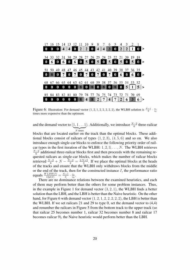
Figure 6: Illustration: For demand vector (1, 2, 1, 2, 2, 2, 2, 2), the WLBH solution is N+13 · z1z0

times more expensive than the optimum.

and the demand vector to (1, 1 . . . 1︸ ︷︷ ︸N times

). Additionally, we introduce N−26

three-railcar

blocks that are located earlier on the track than the optimal blocks. These addi-tional blocks consist of railcars of types (1, 2, 3), (4, 5, 6) and so on. We alsointroduce enough single-car blocks to enforce the following priority order of rail-car types in the first iteration of the WLBH: 1, 2, 3, . . . , N . The WLBH retrievesN−26

additional three-railcar blocks first and then proceeds with the remaining re-quested railcars as single-car blocks, which makes the number of railcar blocksretrieved N−2

6+ N − N−2

2= 2·N+2

3. If we place the optimal blocks at the heads

of the tracks and ensure that the WLBH only withdraws blocks from the middleor the end of the track, then for the constructed instance I , the performance ratioequals WLBH(I)

Opt(I)= N+1

3· z1z0

.There are no dominance relations between the examined heuristics, and each

of them may perform better than the others for some problem instances. Thus,in the example in Figure 1 for demand vector (3, 2, 1), the WLBH finds a bettersolution than the LBH, and the LBH is better than the Naive heuristic. On the otherhand, for Figure 6 with demand vector (1, 2, 1, 2, 2, 2, 2, 2), the LBH is better thanthe WLBH. If we set railcars 21 and 29 to type 0, set the demand vector to (4,4)and renumber the railcars in Figure 5 from the bottom track to the upper track (sothat railcar 25 becomes number 1, railcar 32 becomes number 8 and railcar 17becomes railcar 9), the Naive heuristic would perform better than the LBH.

20

5 Managerial insights based on computational stud-ies

As discussed above, planners often rely on experience-based heuristics to organizerailcar retrieval. Therefore, it is important to evaluate the cost reduction potentialof the exact optimization.

In this section, we perform detailed simulations to evaluate the performancesof exact optimization and heuristic solution approaches as well as to work outfurther important managerial insights. We describe the data generation for thesimulation in Section 5.1. Section 5.2 evaluates the average performances of theintuitive heuristics. In Section 5.3, we examine the impact of a widespread organi-zational routine of presorting on the retrieval costs. At several yards, a lot of timeand resources are devoted to presorting railcars on the storage tracks according totheir types. Section 5.4 evaluates how the yard layout impacts the railcar retrievalcost.

We perform our experiments on a Lenovo notebook with a 2 × 2.3 GHz Inteli5 CPU, 8 GB RAM and Windows 8.1 operating system. The heuristics wereprogrammed with Java 1.8.0, while the RRT-model (1)-(6) is set in Python 3.5.1and solved exactly with Gurobi 6.5.0. We refer to the performance of Gurobi 6.5.0as the MIP, meaning that the Mixed-Integer Program was solved to optimality.

5.1 Simulation settingsThere are different constellations of storage tracks. There are yards with severaldozens of short tracks of about 200 meters in length, and there are yards withfewer, i.e., 20 to 30, long tracks of 800-900 meters in length. In our simulation,we emulate a yard with 25 long tracks. We additionally examine alternative yardlayouts in Section 5.4.

The length of a freight railcar, the so-called length over buffers, ranges from10.6 meter (e.g. for a short Gs model) to 27 meter (e.g. for double-stack rail-cars transporting automobiles). Most railcars are about 14 meters long; thus, a850-meter track may host up to 60 railcars. However, railcars rarely fill all theavailable pitches on the storage tracks, and as a rule, about 50% of pitches arefree. Therefore, in our simulation, we assume that each track contain 30 railcarsand that 25 · 30 = 750 railcars are available on the storage tracks.

Typically, five types of railcar account for approximately 90% of railcars, andthe most widespread type accounts for approximately one third of railcars. Theoverwhelming majority of types contain only one railcar each. We closely cali-brate the data we observed in practice. We generate 50 types of railcar from thedistribution as shown in Figure 7. The prevalence of each of the forty most seldom

21

Figure 7: Probability density of types on the storage tracks used in the simulation

types is set to 0.1%. The distribution of the ten most widespread types follows adiscretized truncated normal distribution with the highest prevalence set to 30%for type 1 (see Figure 7). The probability of a railcar being one of the frequenttypes (1, 2, 3, 4 or 5) is 90% in our distribution, as observed in practice. In oursimulation, we randomly draw a type for each of the 750 railcars on the storagetracks from the distribution described in Figure 7. There are many more theoreti-cally possible railcar types in practice, but this generation method quite accuratelyemulates the number of different types that are simultaneously present on storagetracks.

We refer to the scenario where each railcar may take any position on the stor-age tracks with an equal probability as random. When railcars arrive at the storagetracks, their trains typically consist of only a few types of railcar. Therefore, en-countering conglomerates of railcars of the same type is very likely. We emulatethis situation in our main scenario and designate it default. We re-arrange the gen-erated railcars on the storage tracks so that each railcar has the same type as itsfollower with probability γ provided that railcars of this type are still available.We set γ = 91% so that, if there are enough railcars of a certain type, the averagelength of a homogeneous-type sequence equals 10 railcars.

In Sections 5.2, 5.3 and 5.4, we introduce eight additional scenarios to mimicdifferent settings that are relevant to practice.

A typical order consists of 20 to 40 railcars. Therefore, we set the numberof requested railcars to N = 30. The type of each railcar in the order is ran-domly generated according to the frequency of the types currently available onthe storage tracks.

We set z0 = 1 and z1 = 2 and generate 100 RRT-instances for each scenarioor 100 · 10 = 1, 000 instances in total.

5.2 Performance of the heuristic solution approachesOverall, the retrieval costs for the instances in the random scenario are differentfrom those for the instances in the default scenario. For example, random in-

22

Optimal solutionRetrieval Number of

costs retrieved Relative optimality gap [%]scenario [cost units] blocks Naive LBH WLBH

averagerandom 5.03 3.67 372 64 51default 6.75 5.02 129 45 30

maximumrandom 11.00 7.00 867 200 167default 12.00 8.00 400 200 200

Table 1: Comparative performance of the heuristics for default and random scenarios

Figure 8: The average retrieval costs for the MIP and the WLBH for different order sizes in thedefault scenario

stances tend to contain longer blocks of the requested railcars than the defaultinstances. Therefore, an optimal solution in the random scenario consists of 3.67railcar blocks and that in the default scenario consists of 5 blocks on average (seeTable 1).

Table 1 clearly shows that all of the heuristics lead to highly inflated railcarretrieval costs. The average relative optimality gaps in the default scenario are129%, 45% and 30% for the Naive heuristic, the LBH and the WLBH, respec-tively. Although the WLBH outperforms the LBH and is significantly better thanthe Naive heuristic in our simulation, it still misses the optimality by 30-51%depending on the scenario.

Additionally, we solved the default scenario for order sizes of N = 15 andN = 60. Figure 8 shows the results for these instances provided by the MIPand the WLBH. One can see that the average cost for retrieving the railcars in-creases more strongly with increasing order size for the WLBH solution than forthe optimal solutions.

Because the average computation times of all three heuristics and of the MIP

23

Figure 9: Distribution of the optimal retrieval costs for default and sorted scenarios

are well below one second, we strongly recommend applying the exact optimiza-tion in practice. Indeed, the maximum computation time of the MIP in our exper-iments amounted to 35 seconds for one of the instances. However, this result wasa very unusual outlier.

5.3 Presorting railcars by type and the retrieval costAt several yards, railcars are presorted according to type. This process is ex-tremely expensive and time consuming. To avoid disturbing retrieval operationsand the arrival of railcars, presorting is usually performed during night shifts. Amajor argument in favor of presorting is that it may decrease the variance in thetime required to retrieve the ordered railcars. Indeed, the retrieval costs with thisorganizational policy can never exceed T · z1, and because usually only a fewtypes are requested, i.e. T < N , the case of an extremely long retrieval cost ofN · z1 becomes less likely. However, the expected retrieval time may increase. Asfollows from our analysis in Section 3.2, unless all the railcars of some type cur-rently available on the storage tracks are requested, the retrieval costs can neverfall below

⌈T2

⌉· z0 in the case of presorting. Therefore, for informed manage-

rial decisions, it is extremely important to visualize risk profiles with and withoutpresorting.

We formulate an additional scenario denoted sorted in which all the railcarson the storage tracks are sorted according to type. Note that sorted in this contextmeans that all railcars of one type are placed in sequence (or in two sequencesif the remaining slots on the track are not sufficient to host all the railcars of thistype).

Figure 9 compares the risk profiles for the generated default and sorted in-stances as a boxplot. The whiskers indicate the largest and smallest shunting coststhat have been observed. The box contains the second and third quartile, and the

24

Figure 10: The relation between the average retrieval cost and the number of tracks for differentcost ratios

median is indicated as a horizontal bar in the box. Our simulation shows that,in contrast to the common intuition, the sorted scenario does not only lead to ahigher average retrieval cost but also does not reduce its variance.

However, the average performance of the WLBH improves in the sorted sce-nario. The relative optimality gap decreases from 30% to 16%. Indeed, theheuristics have only a small degree of freedom to deviate from the optimal ob-jective function value for the sorted instances, especially with a large number ofrequested railcars N , because the probability of finding railcar blocks containingdifferent types is low. Therefore, we find that the sorted scenario is more robusttowards the implementation of different planning approaches, such as planningheuristics instead of exact optimization.

5.4 Different yard layouts and the retrieval costThe number and lengths of the storage tracks have important consequences for thefixed (e.g. investment cost) and variable costs of the rail company.

We expect the retrieval cost to vary for different yard layouts even if we keepthe number of railcars on the storage tracks and the distribution of the railcar typesthe same. There are two conflicting forces at play. On the one hand, the largerthe number of storage tracks, the larger the average number of blocks necessaryfor the retrieval of railcars and the higher the retrieval cost. On the other hand,the larger the number of storage tracks, the higher the probability of “paying” z0to pull out a block of railcars and the lower the retrieval cost. Thus, for a givenratio z1

z0and a given yard size K, there is an optimal number of storage tracks that

minimizes the expected retrieval cost. In this section, we determine this numberin a large-scale simulation study.

Based on the default scenario, we formulate six additional scenarios with dif-

25

ferent yard layouts. We keep the number of railcars on the storage tracks atK = 750 for each scenario. We set the number of tracks to 5, 10, 15, 30, 50and 75, and the number of railcars per track to 150, 75, 50, 25, 15 and 10, respec-tively. Afterwards, we compute the average retrieval cost for z1

z0= 1, 1.5, 2, 3, 4, 5.

Figure 10 shows the optimal number of tracks for each ratio z1z0

.Unless the cost ratio z1

z0is lower than 2, short tracks hosting about 10 railcars

each should be preferred. The long tracks scenario is the option of choice at verylow z1

z0. For example, at z1

z0= 1.5, the lowest average retrieval cost is achieved

with rather short tracks hosting about 15 railcars each.

6 ConclusionIn this article, we formulate the problem of railcar retrieval from storage tracks(RRT) as a mixed-integer linear program. We show that the RRT is NP-hard in thestrong sense but that some of its practice-relevant special cases are polynomiallysolvable. We perform thorough worst- and average-case analyses of the intuitiveheuristic solution approaches that are either utilized in practice or motivated by theobserved planning routines. Our analysis indicates a large cost-reduction potentialfor rail companies if they adopt exact optimization approaches instead of heuristicplanning routines. Thus, even the best performing planning heuristics, the LBHand the WLBH, lead to 30%-65% higher retrieval costs on average and may leadto solutions with up to fourteen times higher costs than the optimal solutions insettings that are common in practice. Based on our simulations, we also concludethat the railcar retrieval from storage tracks results in a practically significant costreduction potential and therefore should be considered in studies on the operationsof maintenance centers.

Our simulations also show that, in contrast to the widespread opinion, railcarpresorting results not only in a higher average retrieval cost but also does notreduce the variance of the retrieval cost or time. Moreover, for moderate ratios of1.5 ≥ z1

z0, storage yard layouts consisting of multiple short tracks lead to lower

average retrieval costs.Future research must explicitly integrate the railcar retrieval from storage tracks

into a wide range of planning problems on rail maintenance operations.

Acknowledgements. The authors cooperated with Dr. Christian Otto at DBSchenker Rail and are very grateful to him for his valuable insights into the plan-ning issues of railcar maintenance.

26

References[1] Blasum U, Bussieck MR, Hochstättler W, Moll C, Scheel HH, Winter T

(1999) Scheduling trams in the morning. Mathematical Methods of Opera-tions Research 49(1):137–148

[2] Boysen N, Fliedner M, Jaehn F, Pesch E (2012) Shunting yard operations:Theoretical aspects and applications. European Journal of Operational Re-search 220(1):1–14

[3] Budai G, Huisman D, Dekker R (2006) Scheduling preventive railway main-tenance activities. Journal of the Operational Research Society 57:1035–1044

[4] Corsi T, Casavant K, Graciano T (2012) A preliminary investigation of pri-vate railcars in north america. Journal of the Transportation Research Forum51(1):53–70

[5] Di Stefano G, Koci ML (2004) A Graph Theoretical Approach to the Shunt-ing Problem. Electronic Notes in Theoretical Computer Science 92:16–33

[6] Doganay K, Bohlin M (2010) Maintenance plan optimization for a trainfleet. In: Ning B, Brebbia CA (eds) Computers in Railways XII, WIT Press,Southampton, pp 349–358

[7] EU (2011) Impact assessment: Roadmap to a single european transport area– towards a competitive and resource efficient transport system. Tech. rep.,EU Commission Staff Working Paper, Bruessels

[8] Garey MR, Johnson DS (1979) Computers and Intractability: A Guide to theTheory of NP-Completeness. W. H. Freeman, San Francisco

[9] Gatto M, Maue J, Mihalák M, Widmayer P (2009) Shunting for Dummies:An Introductory Algorithmic Survey. In: Ahuja R, Möhring R, Zaroliagis C(eds) Robust and Online Large-Scale Optimization, Lecture Notes in Com-puter Science, Springer, Berlin, pp 310–331

[10] Hall RW (2000) Scheduling and facility design for transit railcar mainte-nance. Transportation Research Part A: Policy and Practice 34(2):67–84

[11] Hansmann RS, Zimmermann UT (2008) Optimal sorting of rolling stock athump yards. In: Krebs HJ, Jäger W (eds) Mathematics - Key Technology forthe Future, Springer Berlin / Heidelberg, pp 189–203

27

[12] Hecht M (2007) Schneller auf schienen: Beschleunigung des schienengüter-verkehrs durch zeitgemäßge technik. TU International 59(Januar):24–25

[13] Jacobsen PM, Pisinger D (2011) Train shunting at a workshop area. FlexibleServices and Manufacturing Journal 23(2):156–180

[14] Karp RM (1972) Reducibility Among Combinatorial Problems. In: MillerRW, Thatcher JW (eds) Complexity in Computer Computations, Plenum,New York, pp 85–103

[15] Kobbacy KAH, Murthy DN (eds) (2008) Complex System Maintenance.Springer: Berin

[16] Lidén T (2015) Railway infrastructure maintenance - a survey of plan-ning problems and conducted research. Transportation Research Procedia10:574–583

[17] Lübbecke ME, Zimmermann UT (2005) Shunting Minimal Rail Car Alloca-tion. Computational Optimization and Applications 31(3):295–308

[18] Nicolin J, Nogly L (2013) Gütertransport mit güterwagen im wet-tbewerb - bei steigenden ansprüchen/beanspruchungen. In: IFS-Seminar at Aachen University, Downloaded from http://www.ifs.rwth-aachen.de/veranstaltungen/Seminar2013.html on the 9th of October 2015

[19] Ramond F, Dauzère-Pérès S, de Almeida D (2006) Scheduling moves withinrailcar maintenance centers. In: Proceedings of the 12th IFAC Symposiumon Information Control Problems in Manufacturing

[20] Ramond F, de Almeida D, Dauzère-Pérès S (2006) Enhanced operationscheduling within railcar maintenance centers. In: Proceedings of the 7thWorld Congress on Railway Research

[21] SAG-Gruppe (2015) Anlagealternative eisenbahnwaggon: Transparent -rentabel - zukunftsfähig, downloaded from http://www.railinvest.de/ on the9th of October 2015

[22] Winter T, Zimmermann UT (2000) Real-time dispatch of trams in storageyards. Annals of Operations Research 96(1–4):287–315

28

Appendix: Detailed proof of Property 5Proof. As described in Section 4.3, it is sufficient to consider only the cases wherean optimal solution consists of two blocks. In the following, we provide explana-tions only for the set of instances I ′ with Opt(I ′) = 2 · z0, I ′ ∈ I ′. The proofs forthe cases of Opt(I) = 2 · z1 and Opt(I) = z0 + z1 are equivalent.

To find the largest possible estimate for WLBH(I′)Opt(I′)

for instances I ′ ∈ I ′, welook for instances with the worst possible objective value of the WLBH, i.e. forwhich the WLBH withdraws railcars in the largest possible number of blocks,each with a cost of z1. In the first step, we observe that we may restrict our searchto a narrower class of instances I ′′. In the second step, we will make observationsabout the behavior of the WLBH for this narrower class of instances. Finally,based on these observations, we define constraints and set up an optimizationmodel to find an upper bound on the worst possible objective value of the WLBH.

Step 1. Let us run the WLBH on some instance I ′′. We define I ′′ ⊆ I ′ asthe set of instances for which the WLBH retrieves single-car blocks in the lastiteration after it has withdrawn all the multiple-car blocks (if any). The worstpossible objective value of the WLBH for instances I ′ ∈ I ′ is not larger (worse)than the worst possible objective value of the WLBH for instances I ′′ ⊆ I ′.

Indeed, let us construct a WLBH-worst-case-instance I ′, where the WLBHretrieves a single-car block of a critical type t∗ at some iteration m1 ≥ 1 and amultiple-car block of critical type t∗∗ i some later iteration m2 > m1. Then, wemay modify the instance to have this multiple-car block withdrawn at iterationm1

and this single-car block at iteration m2, respectively, (otherwise introducing nochanges in the solution of the WLBH) by adding a sufficient number of railcarsof type t∗∗ intermittently with railcars of type 0 on the tracks (and increasing thelengths of the tracks if necessary). The optimal objective value and the objectivevalue found by the WLBH for instance I ′ and the constructed instance I ′′ will bethe same. Therefore, the relative performance of the WLBH for the constructedinstance I ′′ is not better than for instance I ′.

In the following, we will talk about instances I ′′ ∈ I ′′. We denote a set ofrailcars belonging to all the optimal solutions of some instance I ′′ as X ∗.

Step 2. The main idea of the proof is the following: At some iteration, forinstance, I ′′ ∈ I ′′, the WLBH withdraws a railcar of some type t∗ that is currentlycritical. We denote the vector of the remaining demand, i.e. of the still requestedrailcars, as (n′1, . . . , n

′T ). There is necessarily a railcar of this type t∗ belonging

to the not yet withdrawn railcars of X ∗. The WLBH always retrieves a largestpossible block of railcars containing the currently critical type. Because X ∗ maycontain all the railcars of the largest block, we will examine the properties of theblocks of not yet withdrawn railcars in X ∗. For this purpose, we introduce severaldefinitions. Afterwards, we formulate two observations.

29

Definition. Let us denote the railcars retrieved by the WLBH up to iterationm inclusively as XWLBH

m . We call a set of successively positioned railcars {i, i+1, . . . , i+ l} ⊆ X ∗, i, . . . , i+ l /∈ XWLBH

m with |{j ∈ {i, i+ 1, . . . , i+ l}|u(j) =t}| ≤ n′t,∀1 ≤ t ≤ T as a remaining block B(l)

m at iteration m.In other words, we receive a remaining block if we delete |XWLBH

m | railcars ofthe corresponding types from X ∗ and take a sequence of successively positionedremaining railcars.

Definition. We say that b remaining optimal blocks at iteration m form a re-maining solution Bm = {B(1 )

m , . . . , B(b)m }, if they do not overlap (B(l)

m ∩ B(l ′)m =

∅, 1 ≤ l , l ′ ≤ b) and contain only still requested railcars(|{j ∈

⋃bl=1B

(l)m |u(j) = t}| = n′t, ∀0 ≤ t ≤ T

). We may alternatively denote an

optimal solution of instance I ′′ as B0, i.e. the remaining solution at iteration 0.The example in Figure 6 has only one optimal solution so that

X ∗ = {52, 53, 54, 69, 70, . . . , 79}. In the first iteration, the WLBH withdraws rail-cars {2, 3, 4}. Thus, we do not need railcars of types 1 and 2 anymore, and we re-move railcars 53, 72 and 76 fromX ∗. In this case, the remaining solution is uniqueand consists of five remaining blocksB1 = {{52}, {54}, {69, 70, 71}, {73, 74, 75},{77, 78, 79}}. However, for some instances I ′′ in some iterations, there may beseveral distinct remaining solutions.

We also introduce additional notation. Let for some instance I ′′ the WLBH re-trieveN1 single-car blocks,N2 blocks with two railcars each, . . ., andNN blockswith N railcars each, where Nf are nonnegative integers for f ∈ N. Recall thatall N1 single-car blocks are retrieved in the last iterations of the WLBH.

Observation 1. Let Bm−1 be a remaining solution, m ≥ 1 and Bm is receivedfrom Bm−1 as a result of iteration m of the WLBH, i.e. Bm−1 contains all but|XWLBH

m (I ′′) \ XWLBHm−1 (I ′′)| elements of Bm.

• If the WLBH retrieves a single-car block at iteration m, then the number ofremaining blocks decreases by one: |Bm| = |Bm−1| − 1.

• If the WLBH retrieves a two-railcar block at iteration m, then the numberof remaining blocks may increase by maximally one: |Bm| ≤ |Bm−1|+ 1.

• If the WLBH pulls out a f -railcar block with f ≥ 3 at iteration m, thenthe number of remaining blocks may maximally increase by f : |Bm| ≤|Bm−1|+ f .

In the following, we will provide justification for Observation 1.Case of a single-car block. Let the WLBH retrieve a single-car block at itera-

tion m ≥ 1. Due to the WLBH algorithm, all of the remaining blocks B(l)m−1 con-

taining a railcar of the currently critical type t∗ are single-car blocks. Therefore,

30

regardless of whether or not the WLBH pulls out one of the remaining blocks, thenumber of remaining railcar blocks decreases by one: |Bm| = |Bm−1| − 1.

Case of an f -railcar block, f ≥ 2. Let the WLBH retrieve an f -block, f ≥ 2.We obtain Bm by deleting exactly one railcar from

⋃bl=1B

(l)m−1, where B(l)

m−1 ∈Bm−1∀1 ≤ l ≤ b, for each railcar retrieved by the WLBH at the iteration m. Ifa deleted railcar is located somewhere in the middle of a multiple-car remainingblock B(l)

m−1, then the number of the remaining blocks increases by one. Becausethe WLBH retrieves an f -railcar block, the number of the remaining blocks mayincrease by up to f : |Bm| ≤ |Bm−1|+ f .

Case of a two-railcar block. Let the WLBH retrieve a two-railcar block. Fromthe paragraph above, it follows that the number of remaining blocks cannot in-crease by more than two: |Bm| ≤ |Bm−1| + 2. We strengthen this bound andshow that the number of remaining blocks cannot actually increase by more thanone. Indeed, at least one of the railcars retrieved by the WLBH at iteration mbelongs to the currently critical type t∗. Because there are no remaining blocksB

(l)m−1 containing type t∗ with more than two railcars (otherwise the WLBH would

retrieve a larger block in this iteration), it is impossible to increase the number ofthe remaining blocks by picking a railcar of type t∗. Therefore, the number ofremaining railcar blocks may maximally increase by one: |Bm| ≤ |Bm−1|+ 1.

Observation 2. Let the WLBH have already retrieved all the multiple-carblocks in the previous iterations and be about to withdraw the first single-car blockin the current iteration m ≥ 1, then

• Any remaining solution Bm−1 contains exactly N1 railcars,

• Any remaining solution Bm−1 consists of exactly N1 remaining blocks.

The first statement of Observation 2 follows straightforwardly from the definitionof the remaining solution because exactly N1 railcars are still requested. For thesecond statement, because the WLBH retrieves a single-car block in each of theremaining iterations, it has to performN1 such iterations. Let a remaining solutionBm−1 consist of N ′ 6= N1 remaining blocks. Then, according to Observation 1,the number of remaining blocks in any remaining solution has to decrease by oneafter each iteration m′ > m of the WLBH, which leads to a contradiction.

Step 3. In the following, we will combine the statements of Observation 1 andObservation 2 and construct an optimization problem to find an upper bound onthe worst possible performance of the WLBH for instances I ′′.

Let the WLBH have already retrieved all the multiple-car blocks in the pre-vious iterations and be about to withdraw the first single-car block in the currentiteration m ≥ 1. From Observation 1, the upper bound on the remaining opti-mal blocks of railcars in a remaining solution Bm−1 is

(2 +

∑Nf=3 f · Nf +N2

)31

because each f - and 2-railcar block may maximally increase the number of theremaining optimal blocks by f and 1 in the course of one iteration, respectively.From Observation 2, N1 ≤

(2 +

∑Nf=3 f · Nf +N2

).

The number of railcars retrieved by the WLBH must be equal to the numberof requested railcars:

∑Nf=1 f · Nf = N .

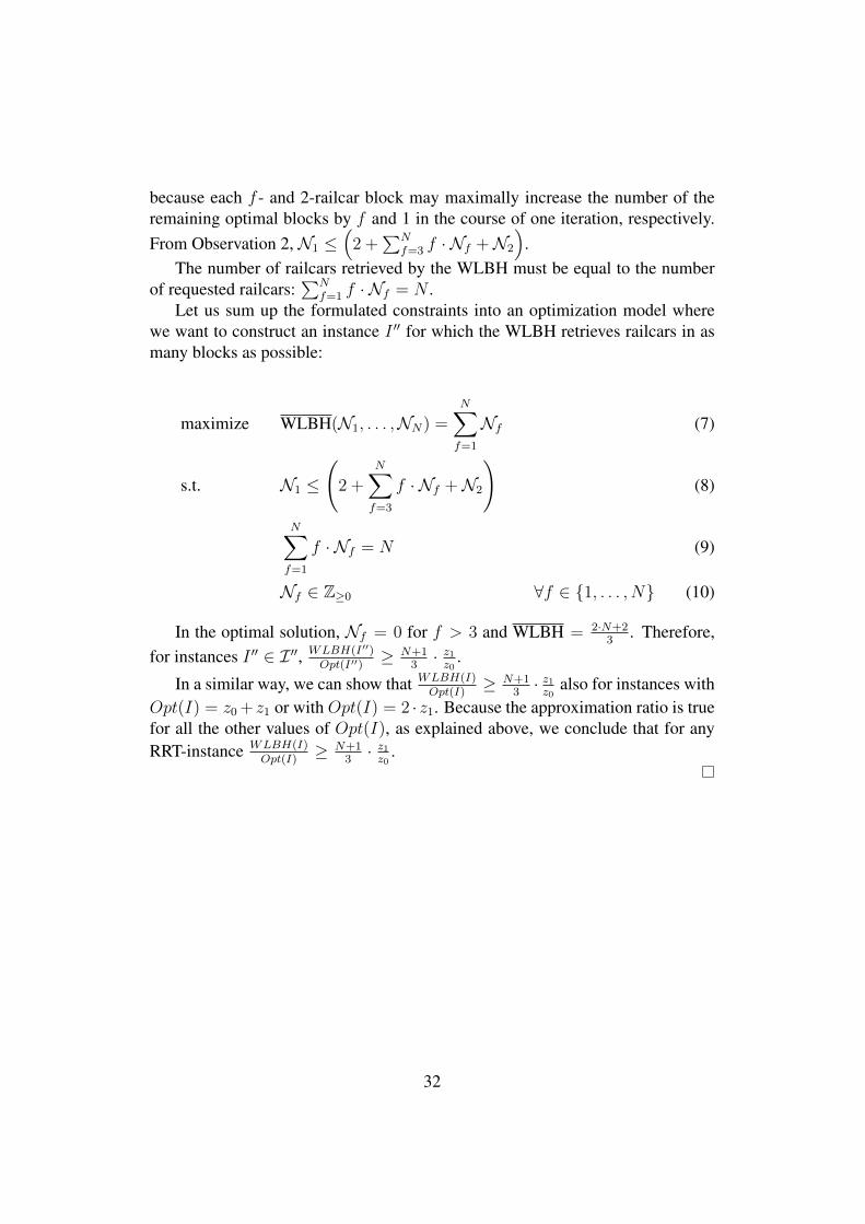
Let us sum up the formulated constraints into an optimization model wherewe want to construct an instance I ′′ for which the WLBH retrieves railcars in asmany blocks as possible:

maximize WLBH(N1, . . . ,NN) =N∑

f=1

Nf (7)

s.t. N1 ≤

(2 +

N∑f=3

f · Nf +N2

)(8)

N∑f=1

f · Nf = N (9)

Nf ∈ Z≥0 ∀f ∈ {1, . . . , N} (10)

In the optimal solution, Nf = 0 for f > 3 and WLBH = 2·N+23

. Therefore,for instances I ′′ ∈ I ′′, WLBH(I′′)

Opt(I′′)≥ N+1

3· z1z0

.

In a similar way, we can show that WLBH(I)Opt(I)

≥ N+13· z1z0

also for instances withOpt(I) = z0+ z1 or with Opt(I) = 2 · z1. Because the approximation ratio is truefor all the other values of Opt(I), as explained above, we conclude that for anyRRT-instance WLBH(I)

Opt(I)≥ N+1

3· z1z0

.

32