Should I Use Fixed or Random E ects? - Data scienceClark... · Should I Use Fixed or Random E ects? Tom S. Clark Associate Professor ... produces bias in estimates of , we consider

Should I Use Fixed or Random Effects?

Tom S. ClarkAssociate Professor

Department of Political ScienceEmory University

[email protected]

Drew A. LinzerAssistant Professor

Department of Political ScienceEmory [email protected]

March 24, 2012

Abstract

Empirical analyses in political science very commonly confront data that are grouped—multiple votes by individual legislators, multiple years in individual states, multipleconflicts during individual years, and so forth. Modeling these data presents a series ofpotential challenges, of which accounting for differences across the groups is perhaps themost well-known. Two widely-used methods are the use of either “fixed” or “random”effects models. However, how best to choose between these approaches remains unclearin the applied literature. We employ a series of simulation experiments to evaluatethe relative performance of fixed and random effects estimators for varying types ofdatasets. We further investigate the commonly-used Hausman test, and demonstratethat it is neither a necessary nor sufficient statistic for deciding between fixed andrandom effects. We summarize the results into a typology of datasets to offer practicalguidance to the applied researcher.

Acknowledgements: We thank Kyle Beardsley, Justin Esarey, Andrew Gelman, BenjaminLauderdale, Jeffrey Lax, and Jamie Monogan for helpful discussions and feedback. Nigel Loprovided valuable research assistance.

1 Introduction

In political science research, it is exceedingly common to confront data that are in some way

grouped. We often have many elections during a given year, multiple survey respondents

from a given state, hundreds of votes made by a single legislator, violent conflicts that take

place within a given country, etc. Indeed, observations in our datasets are often related in

complex ways, involving both nested and non-nested groupings. In our own survey, of the

185 articles published in the American Political Science Review, the American Journal of

Political Science, and the Journal of Politics during 2010, 104 (56%) employed quantitative

data that were in some way grouped.1 The complications that arise when modeling such

data are well known and have received extensive treatment in the econometric and statistical

literatures (e.g., Greene 2008). When modeling such data, perhaps the first question the

applied researcher faces is whether to account for unit effects and, if so, whether to employ so-

called fixed effects or random effects.2 Advice on this topic is plentiful (e.g., Robinson 1998,

Kreft and DeLeeuw 1998, Greene 2008, Kennedy 2003, Frees 2004, Gelman 2005, Wilson and

Butler 2007, Arceneaux and Nickerson 2009, Wooldridge 2010), even if sometimes confusing

and contradictory (Gelman and Hill 2007, 245). However, the implications of this choice

are not always confronted in applied research, and this choice is often made without explicit

attention to how it may affect the quality of inferences to be drawn.

All empirical modeling decisions involve a choice about how to balance variance and

bias. In most quantitative research, this choice is left unstated, but it nevertheless is there.

When modeling data that are grouped and deciding between the use of fixed or random

effects, it is common to place great weight against any perceived level of bias, regardless of

the level of variance implied by that weight. Indeed, it is not uncommon for one to object

1That figure rises to 66% when one excludes the studies that did not employ large-N statistical analyses.2We note there is considerable confusion in the literature concerning the meanings of these terms (for a

discussion, see Gelman 2005, 20). We employ them here as we believe most applied researchers use them—asshorthand for two modeling approaches. As we describe below, fixed effects refer to a series of “dummy”variables for the units from which grouped data arise, while random effects refers to an estimator thatassumes unit effects are drawn from an underlying, modeled distribution.

1

to the use of random effects by noting that if the covariates are correlated with the unit

effects, there may be resulting bias in the parameter estimates. While that claim is true,

it does not imply that any correlation between the covariates and the unit effects implies

fixed effects should be favored. What should be judged instead is how much bias is created,

and how much variance is introduced by using fixed instead of random effects. After all,

except in exceptional circumstances, there will always be some level of correlation between

the covariates and the unit effects, and as a result, at least minimal bias. The question is

how much is too much?

A common approach to resolving this problem is to employ the Hausman test, which

is intended to tell the researcher how significantly parameter estimates differ between the

two approaches. As we demonstrate below, the Hausman test is neither a necessary nor a

sufficient metric for deciding between fixed and random effects. What matters is the size

of the dataset (both number of units and number of observations per unit), the level of

correlation between the covariate and unit effects, and the extent of within-unit variation in

the independent variable relative to the dependent variable.

In this paper, we offer guidance for the applied researcher trying to decide between fixed

and random effects. Many of us are familiar with the basic concepts at play in this decision;

however, we seek to provide practical advice in the form of a systematic analysis of the

implications of the theoretical tradeoff between bias and variance. Indeed, it is our view

that these two fundamental features of the choice researchers face—how to balance bias and

variance; as well as whether econometric specification tests can provide the most relevant

guidance—are general problems that arise regularly in applied research. Below, we review

the basic statistical problems that arise when modeling grouped data and present the results

of a series of Monte Carlo simulation experiments. From those analyses, we derive a set of

basic guidelines by which applied researchers can make effective judgments about how best

to model the relationships of interest in their data.

2

2 The Problem

We consider the linear model for observations i = 1 . . . N grouped into units j = 1 . . . J ,

yi = αj[i] + βxi + εi; εi ∼ N(0, σ2y). (1)

The effect of x on y, denoted β, is the primary quantity of interest. We assume that β is the

same within each unit.3 However, even after accounting for the effect of x, there may still

remain additional variation in the overall level of y across units. The unit effect αj captures

the amount by which predictions of y in unit j must be adjusted upward or downward, given

knowledge only of x. The notation j[i] indicates the unit j of observation i.

One interpretation of the unit effects, αj, is that they represent ignorance about all of

the other systematic factors that predict y, other than x. If these factors were known, they

could ostensibly be included as additional covariates in the model, thus “explaining” the

extra variation in y, and eliminating variation in αj across units. Since these variables are

not included in the model, we capture their effects with αj instead. The variation in αj

might also be partially or completely nonsystematic, due simply to stochastic noise.

With few exceptions, failing to allow for the possibility that αj varies by unit will lead to

biased estimates of β. If we assume that the unit effects are all equivalent—that is, αj = αk

for all j and k—then Equation 1 reduces to the pooled model

yi = α + βxi + εi; εi ∼ N(0, σ2y), (2)

which may be easily estimated by fitting a linear regression to the full dataset, ignoring

information about how observations are grouped into units. The pooled regression model

is appropriate if αj do not vary once x is included as an independent variable. The pooled

3Although there are many instances in which a researcher may wish to allow β to vary by unit, Equation 1represents the most commonly encountered modeling scenario. Our notation follows that of Gelman andHill (2007, 256-257).

3

−4 −2 0 2 4

−4

−2

0

2

4

x

y

Correlation −0.7; pooled β: 0.5

−4 −2 0 2 4

−4

−2

0

2

4

x

y

Correlation 0; pooled β: 1

−4 −2 0 2 4

−4

−2

0

2

4

x

y

Correlation 0.7; pooled β: 1.5

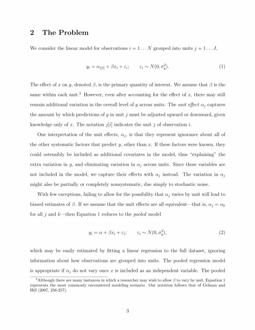
Figure 1: Simulated data showing the effect of correlation between xj and αj on estimatesof β in the pooled regression model. Levels of correlation are -0.7 (left); 0 (center); and0.7 (right). The true β = 1, within ten units each containing 50 observations. Thin linesindicate the underlying, systematic (not estimated) relationship between x and y within eachunit. The result of the pooled regression model is indicated by the thick line. Since β > 1,negative correlation attenuates the estimate of β; positive correlation amplifies it.

model will also not produce bias in estimates of β if the unit effects differ but are uncorrelated

with x. This can occur either if the variation in αj is entirely noise, or if the variables that

predict y but are not included in Equation 1 are all orthogonal to x. Estimating a single α

rather than distinct αj in this particular case would not bias estimates of β because the unit

effects do not confound the relationship between x and y.

More commonly, the unit effects αj are associated with x, so variation in αj must be

modeled in order to avoid faulty inferences about β. To illustrate how the pooled model

produces bias in estimates of β, we consider the magnitude and direction of the correlation

between αj and xj, the mean of x within each unit (Figure 1). If the independent variable

is negatively correlated with the unit effects, then as xj increases, αj decreases. Fitting the

pooled regression model will produce estimates of β < β. When β > 0, this attenuates

estimates of the effect of interest; when β < 0, it makes the estimated effects appear larger

(more negative) than they actually are. When the correlation between xj and αj is positive,

the pooled regression model estimates β > β. For β > 0, the effect of x on y is overestimated;

for β < 0, the effect of x on y is underestimated.

4

3 Two solutions: fixed and random effects

There are two standard approaches for modeling variation in αj: fixed effects and random

effects. The fixed effects model is a linear regression of y on x, that adds to the specification a

series of indicator variables zj for each unit, such that zj[i] = 1 if observation i is in unit j, and

zj[i] = 0 otherwise.4 For example, one may include “year dummies” or “country dummies”

in comparative time series cross-sectional data to account for unexplained year-to-year or

country-to-country variation.

yi =J∑j=1

αjzj[i] + βxi + εi; εi ∼ N(0, σ2y). (3)

The coefficients αj that are computed for each respective zj are taken as estimates of the

“true” unit effects αj.

In the random effects model, the αj are not estimated directly, but are rather assumed

to follow a specified probability distribution; typically normal with mean µα and variance

σ2α. The average unit effect is estimated by µα, and σ2

α describes by how much the other unit

effects vary around that value.

yi = αj[i] + βxi + εi; αj ∼ N(µα, σ2α); εi ∼ N(0, σ2

y). (4)

As Gelman and Hill (2007, 258) note, Equation 4 (the random effects estimator) is equivalent

to Equation 3 (the fixed effects estimator) when we assume that αj ∼ N(µα,∞) rather than

αj ∼ N(µα, σ2α). In other words, the random effects specification models the intercepts

as arising from a distribution with a finite—and estimable—variance σ2α, whereas the fixed

effects specification assumes the intercepts are distributed with infinite variance.5 The pooled

model, by contrast, implicitly assumes σ2α = 0.

4This model is also known as the least squares dummy variable (or LSDV) model.5For this reason, Bafumi and Gelman (2006) advocate the label modeled effects for the random effects

specification and the label unmodeled effects for the fixed effects specification.

5

It is important to clarify that the units in the dataset do not actually have to have been

“drawn” from a larger, normally distributed, population in order to assume a random effects

specification (Greene 2008, 183). We recognize that this statement is at odds with other

sources of econometric advice (e.g., Dougherty 2011). As we will show, however, there is a

range of situations in which the random effects model may be preferable to the fixed effects

model for estimating β, regardless of whether the assumption of “random” effects can be

plausibly said to match the true data generating process.6

3.1 How to choose?

The fixed effects and random effects models both have potential advantages—as well as

disadvantages—to consider when selecting an approach. The fixed effects model will pro-

duce unbiased estimates of β, but those estimates can be subject to high sample-to-sample

variability. The random effects model will, except in rare circumstances, introduce bias in es-

timates of β, but can greatly constrain the variance of those estimates—leading to estimates

that are closer, on average, to the true value in any particular sample. Different researchers

may have different preferences for trading off bias and variance in this manner. More to

the point, the quality of inferences about β under either model can be objectively compared

based upon the size and characteristics of the researcher’s dataset.

The problem of high variance. The estimate of β in the fixed effects model may be

thought of as the average of the within-unit effects of x on y. Under certain conditions, this

estimator may produce estimates that are highly sample-dependent—that is, overly sensitive

to the random error in any given dataset. Suppose that there are few observations per unit,

6There is a third option available, commonly termed the random coefficients model. This model is ageneralization of the random effects model (Equation 4) in which the effect of x on y is allowed to vary byunit as another “random effect”: βj ∼ N(µβ , σ

2β). The mean µβ may then be taken as the estimate of β

in Equation 1. This is a more flexible specification that will tend to produce a closer fit to the observeddata than either the fixed or random effects models. When we extended our simulation study (see below)

to compare the performance of β in the random effects model to µβ in the random coefficients model asestimators of β, we found them to be effectively equivalent. For that reason, we do not investigate therandom coefficients model any further in this paper.

6

or that x does not vary much within each unit, relative to the amount of variation in y.

In that case, estimates of the within-unit effects of x on y can diverge considerably from

the true effect due to chance alone.7 If, in addition, there are a relatively small number of

units, then it becomes increasingly possible for all of the within-unit effects to diverge from

the true effects in the same direction. Under these conditions, the estimate of β produced

by the fixed effects model can be quite different from the true β. This lack of robustness

to potentially anomalous samples is what is meant by the fixed effects model having high

variance.

A related drawback of fixed effects models is that they require the estimation of a pa-

rameter for each unit—the coefficient on the unit dummy variable. This can substantially

reduce the model’s power and increase the standard errors of the coefficient estimates. For

example, if we only observe three elections per country, but have 50 countries in our analysis,

we will have trouble estimating the relationship between the covariate of interest and the

election outcome, because the unit fixed effects will already explain most of the variation

in the dependent variable. Random effects models do not involve the estimation of a set of

dummy variables but instead only the mean and standard deviation of the distribution of

unit effects, saving many degrees of freedom.

Random effects models enable estimation of β with lower sample-to-sample variability by

partially pooling information across units (Gelman and Hill 2007, 258). By estimating the

variance parameter σ2α in Equation 4, the random effects estimator is, in effect, forming a

compromise between the fixed effects and pooled models. Groups with outlying unit effects

will have their respective αj shrunk back towards the mean µα. This brings estimates of β

away from the less-stable fixed effects estimate and closer to the more-stable (albeit poten-

tially biased) pooled estimate. The effects of shrinkage will be greatest for units containing

fewer observations; and especially when estimates of σ2α are close to zero.

7In the bivariate linear regression model, Var(β) increases with smaller values of Var(x), and with largervalues of σ2

y, the conditional variance of y given x (Greene 2008, 48).

7

The problem of bias. The most serious drawback of the random effects approach is the

problem of bias that partial pooling can introduce in estimates of β. To avoid this bias,

the random effects estimator requires the assumption that there is no correlation between

the covariate of interest, x, and the unit effects, αj. An example of such correlation might

arise in a case where the dependent variable is yearly economic growth in a country, and

the explanatory variable is average life expectancy (e.g., Barro 1997). If in some countries,

growth is above or below what would be predicted by life expectancy alone—and in the

countries with above-average unit effects, life expectancy is also longer than average (and

vice-versa)—then this assumption is violated. (This is the scenario depicted in the rightmost

panel of Figure 1.)

More generally, suppose that there is a variable z that predicts y but is not included as

a covariate in the random effects model (Equation 4). As a result of omitting z from the

model specification, the higher or lower levels of y in unit j due to z are accounted for by

the unit effects αj, instead. For there to be no bias in estimates of the coefficient on x,

there must be no correlation between x and z—and, hence, no correlation between x and αj,

implying no confounding due to the omitted z. This bias does not arise in the fixed effects

model because the confounding effect of z on estimates of the effect of x are removed by

estimating separate unit effects. Since the random effects model does not estimate separate

unit effects, any correlation between x and αj can imply an omitted variable z that produces

bias in estimates of β. The greater the magnitude of the correlation between x and αj, the

greater the bias in estimates of β.

Practical considerations. In addition to these theoretical considerations, there are a

number of practical and technical issues which researchers might take into account when

deciding between a fixed effects and random effects estimator. Fixed effects models are

relatively straightforward to implement as an extension of commonly used regression models.

The analyst can simply include a set of dummy variables on the right-hand side of the model.

8

Random effects models, on the other hand, require additional mathematical assumptions.

For researchers who are accustomed to the use of linear regression models, or who may be

unfamiliar with the logic and (potential) benefits of a random effects specification, this small

amount of added complexity could present a barrier to the adoption of a random effects

model. Yet we believe that such barriers are almost always overstated. This is especially

the case given the availability of modern statistical software that makes the random effects

model as easy to estimate as the fixed effects model.

In many situations, the random effects model might even be preferred on practical or

technical grounds. When a dataset contains many units, or is organized according to a

complex data structure (e.g., observations are grouped into more than one unit, or at more

than two levels), random effects models can be much less complicated to specify and interpret

than their fixed effects counterparts.

It is also very common for a researcher to want to include in the specification an important

covariate of interest that does not vary within units (e.g., electoral system type within

countries, or partisan affiliation of legislators). In this case, the unit-invariant predictor

will be perfectly collinear with the set of unit dummy variables, making it impossible to

estimate the unique effects of that variable.8 Alternatively, the independent variable may

exhibit extremely minimal variation within each unit. In data that are time-series cross-

sectional, independent variables that change very gradually over time, particularly relative

to changes in the dependent variable, are frequently referred to as slow-moving or sluggish. If

the correlation between the sluggish covariate and the unit fixed effects is high enough, this

can greatly destabilize estimates of the effect of the independent variable, leading to highly

unreliable inferences. Random effects models are not subject to either of these limitations.

Finally, what if a researcher is interested in using the statistical model to make predictions

about units not included in the dataset? When employing a fixed effects estimator, making

8Plumper and Troeger (2007) propose a three-step modeling approach for data that only vary cross-sectionally; more recently, there has been a reassessment of their approach by Breusch et al. (2011) andGreene (2011), among others.

9

out-of-sample predictions is not possible, because the unit effects for unobserved units are

unknown. In contrast, the random effects model estimates the distribution of unit effects—

including the mean effect—in the broader underlying population. Thus, even if the observed

units are in fact “fixed” (we have a set number of known states, years, etc.), this may be a

reason to prefer a random effects approach.

The Hausman test. Simultaneously incorporating these various theoretical and practical

considerations into model choice may seem a daunting task. As a consequence, to decide

between a random effects and fixed effects model, researchers often rely on the Hausman

(1978) specification test (e.g., Greene 2008, 208-209). The Hausman test is designed to

detect violation of the random effects modeling assumption that the explanatory variables are

orthogonal to the unit effects. If there is no correlation between the independent variable(s)

and the unit effects, then estimates of β in the fixed effects model (βFE) should be similar

to estimates of β in the random effects model (βRE). The Hausman test statistic H is a

measure of the difference between the two estimates:

H = (βRE − βFE)′[Var(βFE)− Var(βRE)

]−1(βRE − βFE). (5)

Under the null hypothesis of orthogonality, H is distributed chi-square with degrees of free-

dom equal to the number of regressors in the model. A finding that p < 0.05 is taken as

evidence that, at conventional levels of significance, the two models are different enough to

reject the null hypothesis, and hence to reject the random effects model in favor of the fixed

effects model.

If the Hausman test does not indicate a significant difference (p > 0.05), however, it

does not necessarily follow that the random effects estimator is “safely” free from bias, and

therefore to be preferred over the fixed effects estimator. In most applications, the true

correlation between the covariates and unit effects is not exactly zero. Thus, if the Hausman

test fails to reject the null hypothesis, it is most likely not because the true correlation is

10

zero—and, hence, that the random effects estimator is unbiased. Rather, it is that the test

does not have sufficient statistical power to reliably detect departures from the null. When

using the random effects model, there will still be bias (if perhaps negligible) in estimates of

β, even if the Hausman test cannot reject the null hypothesis. Of course, in many cases, a

biased estimator (i.e., random effects) can be preferable to an unbiased estimator (i.e., fixed

effects), if the former provides sufficient variance reduction over the latter, as just described.

The Hausman test does not aid in evaluating this tradeoff.

4 Simulation analysis

We perform a series of Monte Carlo experiments to determine the conditions under which a

fixed effects or random effects model provides better estimates of β. Our study investigates

the consequences—and relative importance—of variation in five factors: the number of units,

the number of observations within each unit, the strength of correlation between x and

the unit effects, the strength of association between x and y, and the amount of variation

in x within units. This final factor enables us to manipulate the the sluggishness of the

independent variable, and thus whether the majority of variation in x is located between

units or within units.

To simulate a data-generating process in which observations are clustered by units, we

first generate a series of J within-unit means xj, and corresponding unit effects αj, by

sampling from a bivariate normal distribution centered at zero:

αj

xj

∼ N

0

0

, 1 ρ

ρ 1

. (6)

The variances of both αj and xj are fixed at 1. The off-diagonal covariances ρ control the

amount of correlation between the independent variable and the unit effects. This allows

us to capture both systematic and stochastic sources of variation in αj, without having to

11

Parameter Description Values

J Number of units 10, 40, 100n Observations per unit 5, 20, 50ρ Correlation between independent

variable and unit effects0, 0.1, 0.2, 0.3, 0.4, 0.5, 0.6, 0.7, 0.8, 0.9, 0.95

σx Within-unit standard deviationof x

0.2 (sluggish), 1 (standard)

β Within-unit effect of x on y 0, 0.5, 1, 2

Table 1: Parameters manipulated in the Monte Carlo experiments and their assumed values.

stipulate the omitted factors that might be “causing” the extra variation in y. We then draw

n observations of xi within each unit j = 1 . . . J from a normal distribution with mean xj

and standard deviation σx. The total sample size is J × n. Finally, we apply Equation 1

to produce yi as a linear function of xi, with slope β, unit-level constant terms αj, and

within-unit error variance σ2y = 1.

Our simulations only consider balanced panels in which the number of observations is the

same within each unit. In practice, many political science datasets have unbalanced panels.

In comparative time-series cross-sectional analyses, this frequently occurs as a result of un-

even amounts of missing data across countries or years. Alternatively, there may be unequal

numbers of survey respondents within U.S. states, or differing numbers of terms in office for

elected representatives, for example. We performed an extended set of simulations to assess

the effects of unbalanced panels, and found that these datasets performed equivalently to bal-

anced panels containing the average number of observations per unit. This quantity, rather

than the minimum or maximum number of observations per unit in unbalanced panels, is

what should be used to map one’s actual datasets onto the results we present here.

We choose hypothetical values of J , n, ρ, σx, and β to mimic typical features of quanti-

tative political science datasets (Table 1). In comparative politics research where the units

are countries, for example, the number of democracies is between J = 70 and J = 120; the

number of OECD member countries is J = 34; and the number of countries in (say) South

America is J = 12. In American politics, studies may be concerned with repeated observa-

tions of justices of the Supreme Court (J = 9 units), the set of U.S. states (J = 50 units),

12

−4 −2 0 2 4

−4

−2

0

2

4

x

y

Standard Case

−4 −2 0 2 4

−4

−2

0

2

4

x

y

Sluggish Case

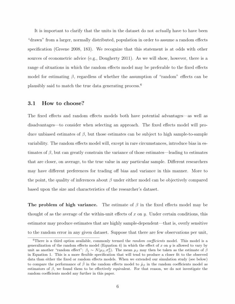
Figure 2: Simulated datasets illustrating variation in σx. Black lines indicate the true rela-tionship between x and y, and span the range of x within each unit. The standard case (left)assumes σx = 1, producing wide variation in x within units, and a large amount of simi-larity between units. The sluggish case (right) constrains σx = 0.2, making the units moredissimilar. In both, β = 1 and ρ = 0, for J = 10 units and n = 50 observations per unit.

or individual Senators (J = 100 units). We vary the number of observations per unit from

n = 5 to n = 50. A dataset that might have very few observations per unit could examine

yearly economic performance grouped by president (n = 4 or n = 8). By contrast, one might

want to analyze behavior of legislators grouped by country (n = 100 or more observations

per unit). In the terminology of longitudinal data analysis, our simulations thus assess both

short panels, in which J > n, as well as long panels, in which n > J .

To control the nature of the variation in x, we set σx = 0.2 for the case of a sluggish

independent variable, and σx = 1 for what we refer to as the standard case (Figure 2). As

noted, the sluggishness of an independent variable refers to the extent to which its within-unit

variation is small relative to the dependent variable. Thus, to manipulate the sluggishness

of the regressor, we hold the conditional variance of y constant and only manipulate the

variance of x. In each graph, the simulated data are plotted with a line segment that spans

the observed range of x within each unit and indicates the underlying relationship between x

and y. In the standard case, there is considerable overlap between the units; in the sluggish

case, there is much less within-unit variation in x. The sluggish case captures instances

where most of the variation in the independent variable is between rather than within units.

13

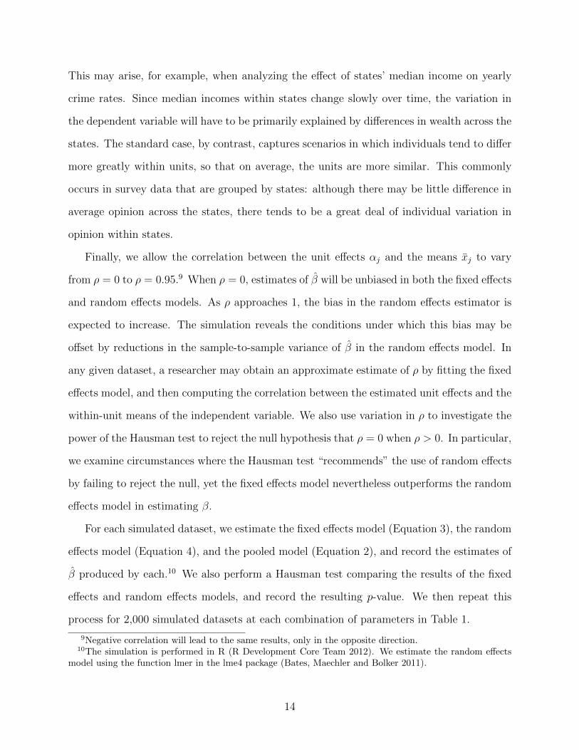
This may arise, for example, when analyzing the effect of states’ median income on yearly

crime rates. Since median incomes within states change slowly over time, the variation in

the dependent variable will have to be primarily explained by differences in wealth across the

states. The standard case, by contrast, captures scenarios in which individuals tend to differ

more greatly within units, so that on average, the units are more similar. This commonly

occurs in survey data that are grouped by states: although there may be little difference in

average opinion across the states, there tends to be a great deal of individual variation in

opinion within states.

Finally, we allow the correlation between the unit effects αj and the means xj to vary

from ρ = 0 to ρ = 0.95.9 When ρ = 0, estimates of β will be unbiased in both the fixed effects

and random effects models. As ρ approaches 1, the bias in the random effects estimator is

expected to increase. The simulation reveals the conditions under which this bias may be

offset by reductions in the sample-to-sample variance of β in the random effects model. In

any given dataset, a researcher may obtain an approximate estimate of ρ by fitting the fixed

effects model, and then computing the correlation between the estimated unit effects and the

within-unit means of the independent variable. We also use variation in ρ to investigate the

power of the Hausman test to reject the null hypothesis that ρ = 0 when ρ > 0. In particular,

we examine circumstances where the Hausman test “recommends” the use of random effects

by failing to reject the null, yet the fixed effects model nevertheless outperforms the random

effects model in estimating β.

For each simulated dataset, we estimate the fixed effects model (Equation 3), the random

effects model (Equation 4), and the pooled model (Equation 2), and record the estimates of

β produced by each.10 We also perform a Hausman test comparing the results of the fixed

effects and random effects models, and record the resulting p-value. We then repeat this

process for 2,000 simulated datasets at each combination of parameters in Table 1.

9Negative correlation will lead to the same results, only in the opposite direction.10The simulation is performed in R (R Development Core Team 2012). We estimate the random effects

model using the function lmer in the lme4 package (Bates, Maechler and Bolker 2011).

14

5 The Hausman Test

We begin by considering the results of our simulation of the Hausman test, in both the

standard case (Figure 3), and the sluggish case (Figure 4), for datasets of varying sizes. The

horizontal axes show the true level of correlation between the covariates and the unit effects;

the vertical axes show the p-values obtained from the Hausman test. The black lines indicate

the average p-value across the simulated datasets. Gray areas show 80% of the Hausman test

p-values at each level of ρ. The horizontal dotted line corresponds to p = 0.05; the point at

which one would traditionally infer that the Hausman test has rejected the null hypothesis,

and thus also rejected the random effects specification.

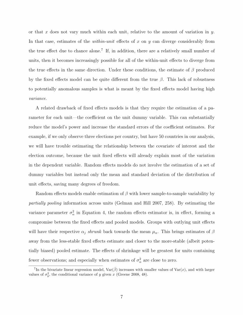
The common belief that the Hausman test will reject the random effects model (p < 0.05)

if there is any correlation between covariates and unit effects is clearly shown to be incorrect.

When the number of units or the number of observations per unit is small—especially when

the covariate is sluggish—the Hausman test will typically fail to reject the random effects

specification, sometimes when the correlation between the predictors and the units is as high

as 0.95. In the top row of Figure 3, we see that for any number of observations per unit, with

only 10 units in the dataset, the Hausman test does not reject the random effects specification

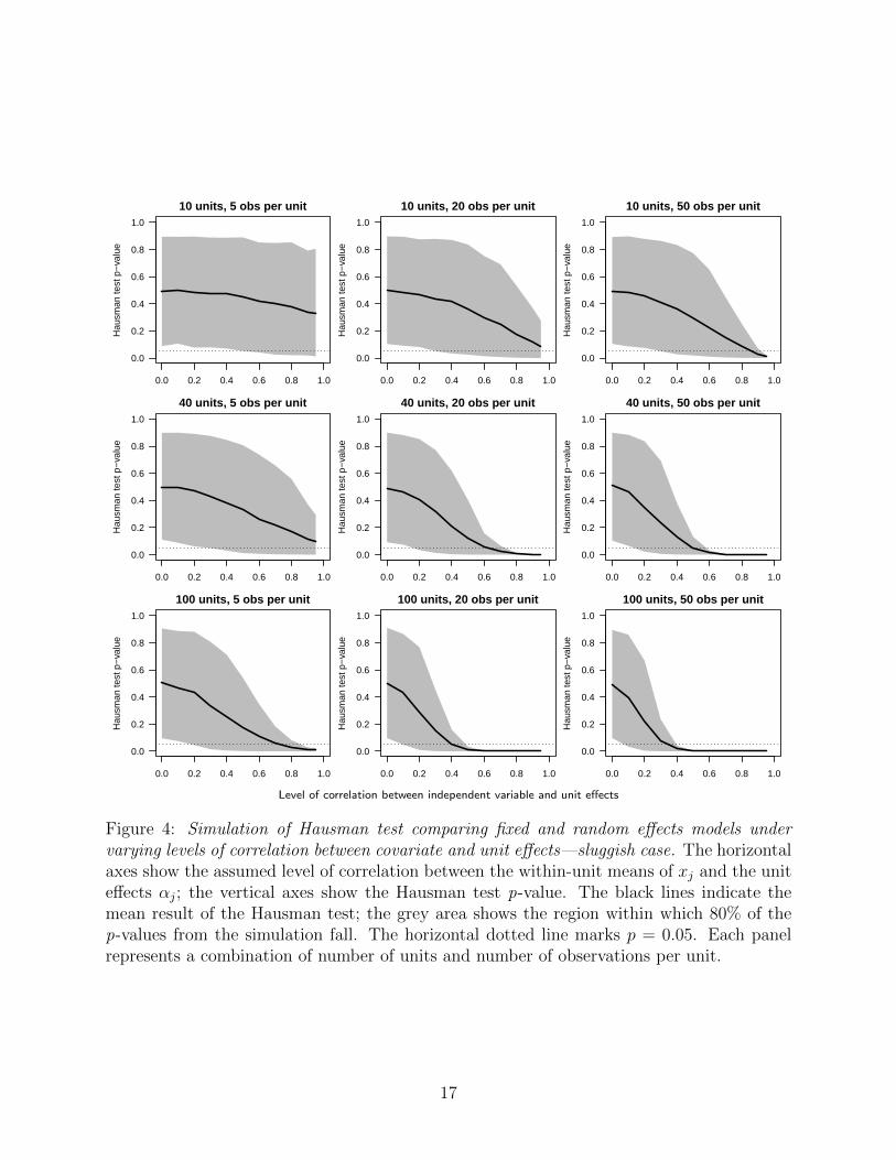
for correlation as high as 0.80. In Figure 4, we see that in the sluggish case, if there are fewer

than 200 total observations, the Hausman test does not reject the random effects specification

(on average) for any level of correlation. For the Hausman test to consistently reject the null

hypothesis, it requires both a large amount of data (here, at least 5,000 observations) and

moderately high correlation between x and the unit effects; perhaps ρ = 0.3 or above. The

results of the Hausman test should not be used to make a binary decision about whether or

not the random effects model will produce bias in estimates of β.

It is our contention, though, that focusing on whether there is any correlation between

the covariate and the unit effects, and thus whether the application of a random effects

estimator results in biased coefficient estimates, is not the correct framework within which

to make a decision about fixed or random effects. The appropriate question to ask, instead,

15

●

0.0 0.2 0.4 0.6 0.8 1.0

0.0

0.2

0.4

0.6

0.8

1.0

10 units, 5 obs per unit

Correlation: unit means and effects

Hau

sman

test

p−

valu

e

●

0.0 0.2 0.4 0.6 0.8 1.0

0.0

0.2

0.4

0.6

0.8

1.0



Hau

sman

test

p−

valu

e

●

0.0 0.2 0.4 0.6 0.8 1.0

0.0

0.2

0.4

0.6

0.8

1.0



Hau

sman

test

p−

valu

e●

0.0 0.2 0.4 0.6 0.8 1.0

0.0

0.2

0.4

0.6

0.8

1.0



Hau

sman

test

p−

valu

e

●

0.0 0.2 0.4 0.6 0.8 1.0

0.0

0.2

0.4

0.6

0.8

1.0



Hau

sman

test

p−

valu

e

●

0.0 0.2 0.4 0.6 0.8 1.0

0.0

0.2

0.4

0.6

0.8

1.0



Hau

sman

test

p−

valu

e

●

0.0 0.2 0.4 0.6 0.8 1.0

0.0

0.2

0.4

0.6

0.8

1.0


Hau

sman

test

p−

valu

e

●

0.0 0.2 0.4 0.6 0.8 1.0

0.0

0.2

0.4

0.6

0.8

1.0


Hau

sman

test

p−

valu

e

●

0.0 0.2 0.4 0.6 0.8 1.0

0.0

0.2

0.4

0.6

0.8

1.0


Hau

sman

test

p−

valu

e

Level of correlation between independent variable and unit effects

Figure 3: Simulation of Hausman test comparing fixed and random effects models undervarying levels of correlation between covariate and unit effects—standard case. The horizon-tal axes show the assumed level of correlation between the within-unit means of xj and theunit effects αj; the vertical axes show the Hausman test p-value. The black lines indicatethe mean result of the Hausman test; the grey area shows the region within which 80% ofthe p-values from the simulation fall. The horizontal dotted line marks p = 0.05. Each panelrepresents a combination of number of units and number of observations per unit.

16

●

0.0 0.2 0.4 0.6 0.8 1.0

0.0

0.2

0.4

0.6

0.8

1.0



Hau

sman

test

p−

valu

e

●

0.0 0.2 0.4 0.6 0.8 1.0

0.0

0.2

0.4

0.6

0.8

1.0



Hau

sman

test

p−

valu

e

●

0.0 0.2 0.4 0.6 0.8 1.0

0.0

0.2

0.4

0.6

0.8

1.0



Hau

sman

test

p−

valu

e●

0.0 0.2 0.4 0.6 0.8 1.0

0.0

0.2

0.4

0.6

0.8

1.0



Hau

sman

test

p−

valu

e

●

0.0 0.2 0.4 0.6 0.8 1.0

0.0

0.2

0.4

0.6

0.8

1.0



Hau

sman

test

p−

valu

e

●

0.0 0.2 0.4 0.6 0.8 1.0

0.0

0.2

0.4

0.6

0.8

1.0



Hau

sman

test

p−

valu

e

●

0.0 0.2 0.4 0.6 0.8 1.0

0.0

0.2

0.4

0.6

0.8

1.0


Hau

sman

test

p−

valu

e

●

0.0 0.2 0.4 0.6 0.8 1.0

0.0

0.2

0.4

0.6

0.8

1.0


Hau

sman

test

p−

valu

e

●

0.0 0.2 0.4 0.6 0.8 1.0

0.0

0.2

0.4

0.6

0.8

1.0


Hau

sman

test

p−

valu

e


Figure 4: Simulation of Hausman test comparing fixed and random effects models undervarying levels of correlation between covariate and unit effects—sluggish case. The horizontalaxes show the assumed level of correlation between the within-unit means of xj and the uniteffects αj; the vertical axes show the Hausman test p-value. The black lines indicate themean result of the Hausman test; the grey area shows the region within which 80% of thep-values from the simulation fall. The horizontal dotted line marks p = 0.05. Each panelrepresents a combination of number of units and number of observations per unit.

17

is how much bias results—and whether the resulting bias can be justified by the gain in

efficiency. Rather than place absolute weight on any bias relative to the amount of weight

put on efficiency, one should decide how to balance bias and efficiency.

6 Comparing model quality

As noted above, all modeling choices involve balancing bias and variance; the critical question

is how much bias one is willing to tolerate and at what expense in variability. To this end, we

advocate comparing the two quantities directly. Objecting to a random effects specification

solely out of concern for bias in the parameter estimates does not adequately address the

underlying criterion by which model choice is made. As our simulations reveal, in many

cases the total root mean squared error (RMSE) of estimates of β is lower with random

effects than with fixed effects, even if the random effects estimate is somewhat biased.

6.1 Assessing bias

We consider the amount of bias in estimates of the slope β that result from applying a fixed

effects, random effects, or pooled estimator under varying amounts of correlation between

the independent variable and the unit effects. At each sample size and level of correlation,

we calculate the average value of β across the set of simulated datasets. The true value

of β in these simulations is set at 1. We repeat this simulation for both the standard case

(Figure 5) and the sluggish case (Figure 6).

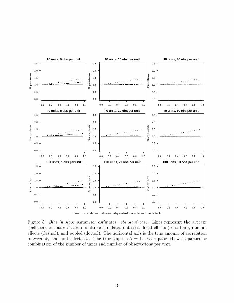
The fixed effects estimator, on average, always recovers the true slope parameter estimate—

it is always right at 1. At the same time, though, increasing the number of observations per

unit always decreases the bias in the random effects estimate, independent of the number

of units. In each column, moving from left to right (increasing the observations per unit)

brings the estimated slope parameter closer to the true slope. In fact, in our simulations of

the standard case, once there are at least 20 observations per unit, there is hardly any bias in

18

0.0 0.2 0.4 0.6 0.8 1.0

0.0

0.5

1.0

1.5

2.0

2.5



Slo

pe e

stim

ate

0.0 0.2 0.4 0.6 0.8 1.0

0.0

0.5

1.0

1.5

2.0

2.5



Slo

pe e

stim

ate

0.0 0.2 0.4 0.6 0.8 1.0

0.0

0.5

1.0

1.5

2.0

2.5



Slo

pe e

stim

ate

0.0 0.2 0.4 0.6 0.8 1.0

0.0

0.5

1.0

1.5

2.0

2.5



Slo

pe e

stim

ate

0.0 0.2 0.4 0.6 0.8 1.0

0.0

0.5

1.0

1.5

2.0

2.5



Slo

pe e

stim

ate

0.0 0.2 0.4 0.6 0.8 1.0

0.0

0.5

1.0

1.5

2.0

2.5



Slo

pe e

stim

ate

0.0 0.2 0.4 0.6 0.8 1.0

0.0

0.5

1.0

1.5

2.0

2.5


Slo

pe e

stim

ate

0.0 0.2 0.4 0.6 0.8 1.0

0.0

0.5

1.0

1.5

2.0

2.5


Slo

pe e

stim

ate

0.0 0.2 0.4 0.6 0.8 1.0

0.0

0.5

1.0

1.5

2.0

2.5


Slo

pe e

stim

ate


Figure 5: Bias in slope parameter estimates—standard case. Lines represent the averagecoefficient estimate β across multiple simulated datasets: fixed effects (solid line), randomeffects (dashed), and pooled (dotted). The horizontal axis is the true amount of correlationbetween xj and unit effects αj. The true slope is β = 1. Each panel shows a particularcombination of the number of units and number of observations per unit.

19

0.0 0.2 0.4 0.6 0.8 1.0

0.0

0.5

1.0

1.5

2.0

2.5



Slo

pe e

stim

ate

0.0 0.2 0.4 0.6 0.8 1.0

0.0

0.5

1.0

1.5

2.0

2.5



Slo

pe e

stim

ate

0.0 0.2 0.4 0.6 0.8 1.0

0.0

0.5

1.0

1.5

2.0

2.5



Slo

pe e

stim

ate

0.0 0.2 0.4 0.6 0.8 1.0

0.0

0.5

1.0

1.5

2.0

2.5



Slo

pe e

stim

ate

0.0 0.2 0.4 0.6 0.8 1.0

0.0

0.5

1.0

1.5

2.0

2.5



Slo

pe e

stim

ate

0.0 0.2 0.4 0.6 0.8 1.0

0.0

0.5

1.0

1.5

2.0

2.5



Slo

pe e

stim

ate

0.0 0.2 0.4 0.6 0.8 1.0

0.0

0.5

1.0

1.5

2.0

2.5


Slo

pe e

stim

ate

0.0 0.2 0.4 0.6 0.8 1.0

0.0

0.5

1.0

1.5

2.0

2.5


Slo

pe e

stim

ate

0.0 0.2 0.4 0.6 0.8 1.0

0.0

0.5

1.0

1.5

2.0

2.5


Slo

pe e

stim

ate


Figure 6: Bias in slope parameter estimates—sluggish case. Lines represent the averagecoefficient estimate β across multiple simulated datasets: fixed effects (solid line), randomeffects (dashed), and pooled (dotted). The horizontal axis is the true amount of correlationbetween xj and unit effects αj. The true slope is β = 1. Each panel shows a particularcombination of the number of units and number of observations per unit.

20

the slope parameter, for any level of correlation between the covariate and the unit effects.

Even when correlation between the covariate and the unit effects is greater than 0.9, the

estimated slope parameter from the random effects specification is effectively equivalent to

the true slope parameter. Instead, it is only when there are very little data (specifically, five

or fewer observations per unit) does correlation between the covariate and the unit effects

result in any appreciable bias in the standard case.

In the sluggish case, when there is more variation across units than within units, the

random effects estimator fares less well, resulting in more bias in the estimate of β. As with

the standard case, more data leads to less biased estimates. Interestingly, though, increasing

the number of units does not affect the amount of resulting bias; instead bias is decreased

by increasing the number of observations per unit. Thus, when dealing with a sluggish

covariate, observing more units (for example, adding more legislators to one’s data) will not

result in an improvement of the estimate of β; instead one should try to increase the number

of observations observed (for example, adding more votes by each legislator).

The pooled estimator is always more biased than either the random effects or fixed effects

estimator, and—unlike the random effects model—increasing the amount of data (units,

observations per unit, or both) does not affect the extent of the bias. Rather, the bias is

driven purely by the level of correlation between the regressor and the unit effects.

Critically, it is precisely under the condition of little data that the Hausman test is least

likely to reject the random effects specification. Figures 3 and 4 above both show that when

there are little data—particularly in the sluggish case—the Hausman test generally fails

to reject the random effects specification, even when there is high correlation between the

covariate and the unit effects (and, seen in Figures 5 and 6, the most bias in the resulting

parameter estimate). What is more, taken in conjunction, Figures 3 through 6 show that

where the Hausman test is most likely to reject a random effects specification is when there

is some moderate level of correlation (i.e., greater than 0.5) and there is a great deal of data

(i.e., many units and many observations per unit). In the standard case, however, it is under

21

these conditions that there is no discernible difference between the estimates from a fixed

and random effects approach. With at least 20 observations per unit, there is no appreciable

difference in the slope parameter estimate for any level of correlation, even with few units.

6.2 Bias and variance considered jointly

Although the random effects estimator can produce bias in estimates of β, it is also expected

to reduce the sample-to-sample variation in those estimates. To assess the total tradeoff

between bias and variance in the three estimators, we compare the RMSE of β from the

fixed effects, random effects, and pooled models, for the standard case (Figure 7) and the

sluggish case (Figure 8).

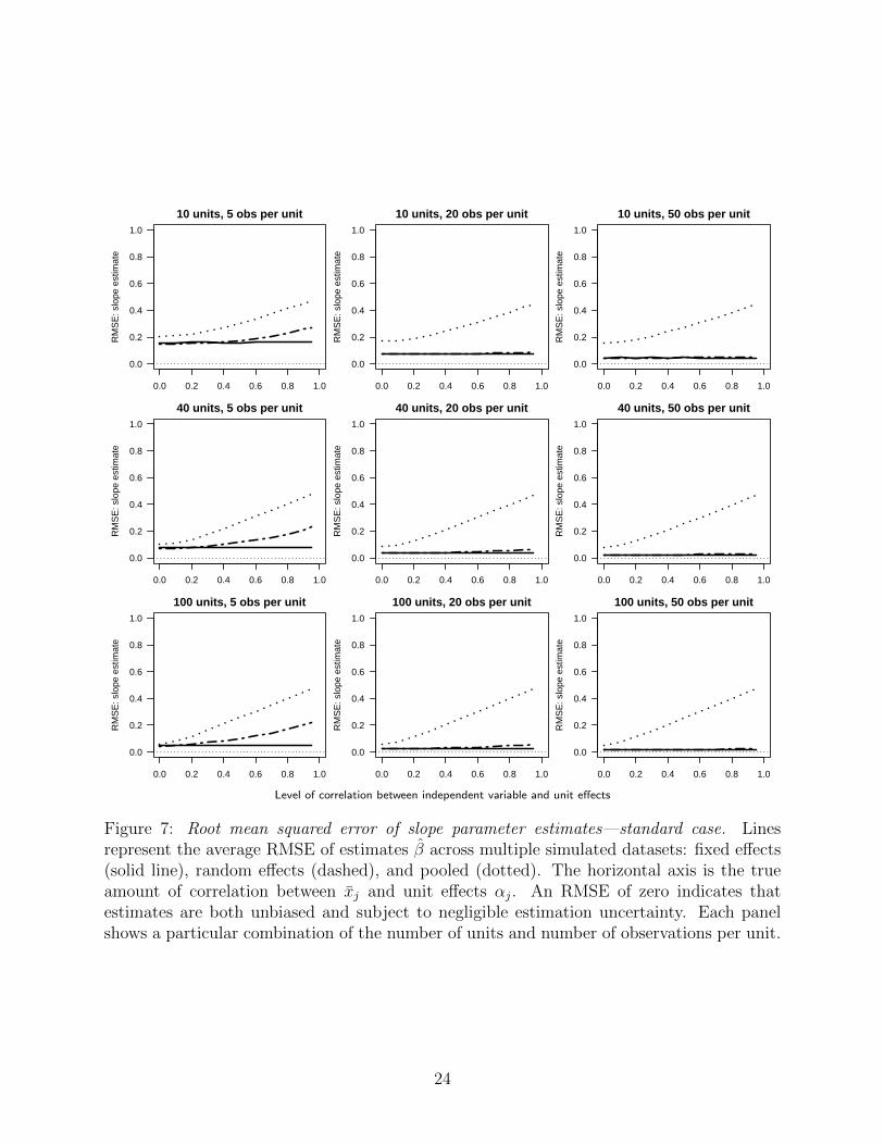
These figures demonstrate an important distinction in how the three estimators’ fits to

the data change as a function of the amount of data and extent of correlation between

the covariate and unit effects. Most important, as we saw above, bias in the fixed effects

estimator’s estimate of β is invariant to the amount of correlation with the unit effects and

the amount of data. Thus, the only source of variation in the RMSE is the variance in β.

Because variance in the fixed effects estimator’s estimate of β strictly decreases with the

amount of data in the sample, the highest RMSE for the fixed effects estimator is in the

case of the fewest units and fewest observations per unit (top left-hand corner). The lowest

RMSE for the fixed effects estimator is in the case of the most units and most observations

per unit (bottom right-hand corner). By contrast, the random effects estimator’s fit to the

data has a more complicated relationship to the amount of data and underlying correlation.

For any given number of units, increasing the number of observations per unit decreases the

random effects RMSE at all levels of correlation. To a lesser extent, increasing the number of

units (while keeping the number of observations per unit constant) also decreases the random

effects RMSE. Finally, under all conditions, the pooled estimator yields a higher RMSE than

the random effects estimator, though it can outperform the fixed effects estimator when the

data are sufficiently sparse.

22

The consequence of these findings is straightforward. While correlation between x and

the unit effects increases the random effects estimator’s RMSE, such an increase does not

necessarily justify preferring the fixed effects estimator. The fewer data one has, the greater

the range of correlation between x and the unit effects that can still justify a random effects

specification. The reason is that the bias induced in the random effects estimate of β by

any given level of correlation is offset by the higher variance of the fixed effects estimate.

Naturally, as the amount of data increases, the extent to which the random effects estimate

yields lower variance will decrease, implying that only lower levels of correlation will result

in a superior estimate from the random effects model.

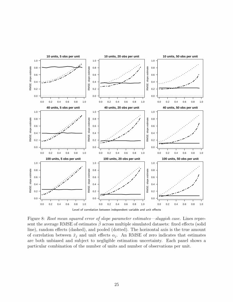
Beyond the effects of the amount of data and the extent to which the random effects

estimator’s assumptions are violated by correlation between the covariate and the unit effects,

our simulations demonstrate another important finding. The extent to which there is any

difference between the two estimators is also a function of the sluggishness of the covariate.

In the standard case (Figure 7), the fixed effects estimator yields a better RMSE only when

the number of observations per unit is very small (less than 20) and there is relatively high

correlation between the covariate and the unit effects. With only five observations per unit,

the random effects is still superior to the fixed effects estimator for levels of correlation as

high as 0.4.

However, following the general pattern that has been identified throughout our analysis,

it is precisely the conditions under which the Hausman test is most likely to reject a random

effects estimator that the differences between the two estimators is least. When there are

many observations per unit (the right columns in each of the Figures 3 through 8), the

Hausman test is most effective as identifying differences between the two estimators, but it

is also under these conditions that the bias in the random effects estimator is smallest and

the difference in the RMSE between the two estimators is negligible.

Finally, we note that there are conditions under which the random effects estimator is

subject to appreciable bias but still produces better estimates of β on average. Specifically,

23

0.0 0.2 0.4 0.6 0.8 1.0

0.0

0.2

0.4

0.6

0.8

1.0



RM

SE

: slo

pe e

stim

ate

0.0 0.2 0.4 0.6 0.8 1.0

0.0

0.2

0.4

0.6

0.8

1.0



RM

SE

: slo

pe e

stim

ate

0.0 0.2 0.4 0.6 0.8 1.0

0.0

0.2

0.4

0.6

0.8

1.0



RM

SE

: slo

pe e

stim

ate

0.0 0.2 0.4 0.6 0.8 1.0

0.0

0.2

0.4

0.6

0.8

1.0



RM

SE

: slo

pe e

stim

ate

0.0 0.2 0.4 0.6 0.8 1.0

0.0

0.2

0.4

0.6

0.8

1.0



RM

SE

: slo

pe e

stim

ate

0.0 0.2 0.4 0.6 0.8 1.0

0.0

0.2

0.4

0.6

0.8

1.0



RM

SE

: slo

pe e

stim

ate

0.0 0.2 0.4 0.6 0.8 1.0

0.0

0.2

0.4

0.6

0.8

1.0


RM

SE

: slo

pe e

stim

ate

0.0 0.2 0.4 0.6 0.8 1.0

0.0

0.2

0.4

0.6

0.8

1.0


RM

SE

: slo

pe e

stim

ate

0.0 0.2 0.4 0.6 0.8 1.0

0.0

0.2

0.4

0.6

0.8

1.0


RM

SE

: slo

pe e

stim

ate


Figure 7: Root mean squared error of slope parameter estimates—standard case. Linesrepresent the average RMSE of estimates β across multiple simulated datasets: fixed effects(solid line), random effects (dashed), and pooled (dotted). The horizontal axis is the trueamount of correlation between xj and unit effects αj. An RMSE of zero indicates thatestimates are both unbiased and subject to negligible estimation uncertainty. Each panelshows a particular combination of the number of units and number of observations per unit.

24

0.0 0.2 0.4 0.6 0.8 1.0

0.0

0.2

0.4

0.6

0.8

1.0



RM

SE

: slo

pe e

stim

ate

0.0 0.2 0.4 0.6 0.8 1.0

0.0

0.2

0.4

0.6

0.8

1.0



RM

SE

: slo

pe e

stim

ate

0.0 0.2 0.4 0.6 0.8 1.0

0.0

0.2

0.4

0.6

0.8

1.0



RM

SE

: slo

pe e

stim

ate

0.0 0.2 0.4 0.6 0.8 1.0

0.0

0.2

0.4

0.6

0.8

1.0



RM

SE

: slo

pe e

stim

ate

0.0 0.2 0.4 0.6 0.8 1.0

0.0

0.2

0.4

0.6

0.8

1.0



RM

SE

: slo

pe e

stim

ate

0.0 0.2 0.4 0.6 0.8 1.0

0.0

0.2

0.4

0.6

0.8

1.0



RM

SE

: slo

pe e

stim

ate

0.0 0.2 0.4 0.6 0.8 1.0

0.0

0.2

0.4

0.6

0.8

1.0


RM

SE

: slo

pe e

stim

ate

0.0 0.2 0.4 0.6 0.8 1.0

0.0

0.2

0.4

0.6

0.8

1.0


RM

SE

: slo

pe e

stim

ate

0.0 0.2 0.4 0.6 0.8 1.0

0.0

0.2

0.4

0.6

0.8

1.0


RM

SE

: slo

pe e

stim

ate


Figure 8: Root mean squared error of slope parameter estimates—sluggish case. Lines repre-sent the average RMSE of estimates β across multiple simulated datasets: fixed effects (solidline), random effects (dashed), and pooled (dotted). The horizontal axis is the true amountof correlation between xj and unit effects αj. An RMSE of zero indicates that estimatesare both unbiased and subject to negligible estimation uncertainty. Each panel shows aparticular combination of the number of units and number of observations per unit.

25

0.0 0.2 0.4 0.6 0.8 1.0

0.0

0.2

0.4

0.6

0.8

1.0

true slope: 0R

MS

E: s

lope

est

imat

e

0.0 0.2 0.4 0.6 0.8 1.0

0.0

0.2

0.4

0.6

0.8

1.0

true slope: 0.5

RM

SE

: slo

pe e

stim

ate

0.0 0.2 0.4 0.6 0.8 1.0

0.0

0.2

0.4

0.6

0.8

1.0

true slope: 2

RM

SE

: slo

pe e

stim

ate


Figure 9: Root mean squared error of slope parameter estimates for varying effect sizes:β = 0, β = 0.5, and β = 2. Simulated data are for the sluggish case, with 40 units and20 observations per unit. These plots correspond to the central panel of Figure 8, in whichβ = 1. As above, lines indicate results from the fixed effects (solid), random effects (dashed),and pooled (dotted) models.

when there is relatively little data and the correlation between the covariate and the unit

effects is not too high, the random effects estimator will result in some degree of bias, but the

RMSE is considerably better under the random effects estimator than under the fixed effects

estimator. The “better” result is driven by the random effects’ more efficient estimate of the

parameter, which more than compensates for bias in the parameter estimate. This result

underscores our argument that scholars should think more carefully about the bias-variance

tradeoff than is common practice.

6.3 The effect size does not matter

In each of the preceding simulations, we have fixed the within-unit effect of x on y at β = 1.

What if this effect was larger or smaller? To answer this question, we consider values of

β = 0, β = 0.5, and β = 2. We set the number of units at J = 40 and the number of

observations per unit at n = 20. These values correspond to the central panels in Figures 3

through 8. We repeat the simulation and calculate the RMSE under each of the random

effects, fixed effects, and pooled model specifications, for varying levels of correlation between

the independent variable and unit effects. The results exactly match those shown in Figures 7

26

and 8. For brevity, we only show the results for the more interesting sluggish case (Figure 9).

The RMSE of each estimator is invariant to the effect size β.

7 A summary rubric

Our analysis yields a series of general rules of thumb that should guide researchers when

deciding how best to model their data. There are, in our view, three primary considerations:

the extent to which variation in the explanatory variable is primarily within unit (the stan-

dard case) as opposed to across units (the sluggish case), the amount of data one has (the

number of units and observations per unit), and the goal of the modeling exercise. We offer

a general framework for modeling choices by considering the latter two criteria in both the

general and sluggish cases.

The standard case: variation is primarily within units. Consider first the standard

case—where variation in x is primarily within units. Under this condition, there is rarely any

difference between the random effects estimator and the fixed effects estimator. Only when

there is little data and correlation between the regressor and unit effects is exceptionally

high (above 0.9 in our simulations) does the fixed effects estimator outperform the random

effects estimator, as measured by the RMSE. Thus, the conventional understanding that

correlation between regressors and unit effects results in unwarranted bias in the estimate of

the model parameters is unfounded.

Rather, what we find is that any bias in the slope parameter estimate is more than

compensated for by the increase in estimate efficiency. This is true even for small datasets

with large violations of the assumption of zero correlation. In the standard case, then,

our guidance to the researcher is to use whichever model better serves the purpose of the

research. For example, if one potentially wants to make predictions about unobserved units

(for example, judges, legislators or countries not in the dataset), then the random effects

estimator should be used, because the fixed effects estimator cannot make such predictions.

27

Observations per UnitFew (≤ 5) Many

Numberof units

Few (≤ 10) Random effects Random effects if correlation islow; fixed effects otherwise

Many Random effects if correlation islow; fixed effects otherwise

Fixed effects unless correlationis close to zero

Table 2: Summary advice for modeling data with a sluggish independent variable, by numberof units and number of observations per unit in dataset. Each cell represents a combinationof the number of units in a dataset and the number of observations per unit. The entriessummarize the best approach to modeling these data, based on an analysis of when the RMSEfavors the fixed or random effects estimator.

Similarly, if perfect (or near-perfect) collinearity between a regressor of interest and the unit

effects (e.g., a legislator’s political party or a country’s electoral system) precludes the use of

a fixed effects estimator, one should not resist the use of a random effects estimator because

of potential correlation between the regressor and the unit effects.

The sluggish case: variation is primarily across units. Consider next the sluggish

case—where there is little variation in the regressor relative to variation across units. In

this scenario, our advice is more complicated and is summarized in Table 2. In brief, the

best approach to modeling one’s data depends on the amount of the data one has and the

level of correlation between the regressor and unit effects. When there is very little data,

even under extreme violations of the assumption of zero correlation, the random effects

estimator outperforms the fixed effects estimator. When there is a lot of data—many units

and many observations per unit—then one should employ a fixed effects specification when

there is even a moderate level of correlation between the unit effects and the regressor.

When there is an intermediate amount of data—many units but few observations per unit,

or vice-versa—then the better model depends on the underlying level of correlation. With ρ

less than approximately 0.3 to 0.5, in each of our simulations the random effects estimator

outperforms the fixed effects estimator on average. However, with larger levels of correlation,

the fixed effects estimator tends to outperform the random effects estimator.

28

Finally, we note that the pooled estimator is always weakly inferior to the random effects

estimator, and the extent to which the random effects estimator is superior increases as the

number of observations per unit increases. Thus, we find in the sluggish case that, again,

the conventional wisdom that a violation of the random effects model’s assumption of zero

correlation is neither a sufficient nor a necessary condition for choosing a fixed effects model.

Instead, the decision must be determined by the amount of data one has and the underlying

level of correlation between the unit effects and regressor.

8 Conclusion

We set out to provide practical guidance to applied empirical modelers facing a common

dilemma in political science—how to account for unit effects in grouped data. Scholars

generally approach these data by using either “fixed” or “random” effects. While advice

on how to select between these alternatives is plentiful, it is also often contradictory or

inconclusive. Perhaps the most frequent suggestion is to rely on the Hausman test, which

is designed to assess whether there is a significant difference between the estimates of the

two models. If there is not, then the researcher is directed to use random effects, as they

are more efficient than fixed effects. A significant difference, on the other hand, is taken as

evidence of bias in the random effects estimate, and the researcher is consequently guided

to employ fixed effects instead.

Yet our simulations reveal that the Hausman test is not a reliable tool for identifying

bias in typically-sized samples; nor does it aid in evaluating the balance of bias and variance

implied by the two modeling approaches. As we point out, “testing” for bias in the random

effects model implicitly assigns infinite weight to bias at the expense of any possible benefits

due to variance reduction. We see no reason why one should not be willing to accept some

degree of bias in the parameter estimates if it is accompanied by a sufficient gain in efficiency.

29

To best evaluate this tradeoff, we have argued that researchers should rely on a com-

parison of the RMSE of estimates of the effect of x on y between the two models. The

most common objection to the use of random effects—the violation of a “critical” modeling

assumption; that the regressor and the unit effects are uncorrelated—turns out to be an

insufficient justification to prefer fixed over random effects. Only under exceptional circum-

stances will this condition hold, and our simulations demonstrate that even in the presence

of rather extreme violations of that assumption, the random effects estimator can still be

preferable to (or at least no worse than) the fixed effects estimator.

We offer a series of general rules of thumb upon which researchers may rely when choosing

between a fixed effects or random effects approach. When variation in the independent

variable is primarily within units—that is, the units are relatively similar to one another

on average—the choice of random versus fixed effects only matters at extremely high levels

of correlation between the independent variable and the unit effects, and when there are

very few observations per unit (perhaps less than five, on average). With larger amounts

of data—many units and/or observations—there is no discernible difference in estimates of

β between the two estimators, even when the regressor and the unit effects are very highly

correlated. Thus, under these conditions, the appropriate model should be guided by the

researcher’s goals. For example, if one seeks to make predictions abut unobserved units, then

the random effects estimator should be employed.

When the independent variable exhibits only minimal within-unit variation, or is sluggish,

there is a more nuanced set of considerations. In any particular dataset, the random effects

model will tend to produce better estimates of β when there are few units or observations per

unit, and when the correlation between the independent variable and unit effects is relatively

low. Otherwise, the fixed effects model may be preferable because the random effects model

does not induce sufficiently high variance reduction to offset its increase in bias.

Finally, there are important limitations to the guidance offered here. We have not con-

sidered the problem where the researcher hypothesizes that the effect of x on y varies across

30

units, in which case one would need to employ interactive terms (fixed effects approach) or

a random coefficients model (random effects approach). In addition, we have only consid-

ered the linear regression model; we have not contemplated other common models, such as

limited dependent variable models like logit or probit. Nevertheless, the overall approach we

have employed to evaluate the performance of random and fixed effects models under various

violations of the model assumptions can easily be extended to evaluate alternative models

on a case-by-case basis. We believe that applied researchers in the future should follow these

steps when deciding how best to model their data.

31

References

Arceneaux, Kevin and David W. Nickerson. 2009. “Modeling Certainty with Clustered Data:A Comparison of Methods.” Political Analysis 17(2):177–190.

Bafumi, Joseph and Andrew Gelman. 2006. “Fitting Multilevel Models When Predictors andGroup Effects Correlate.” Paper presented at the annual meeting of the Midwest PolititcalScience Association, Chicago, IL.

Barro, Robert J. 1997. Determinants of Economic Growth: A Cross-Country EmpiricalStudy. Cambridge, MA: MIT Press.

Bates, Douglas, Martin Maechler and Ben Bolker. 2011. lme4: Linear mixed-effects modelsusing S4 classes. R package version 0.999375-38. http://cran.R-project.org/package=lme4.

Breusch, Trevor, Michael B. Ward, Hoa Thi Minh Nguyen and Tom Kompas. 2011. “On theFixed-Effects Vector Decomposition.” Political Analysis 19(2):123–134.

Dougherty, Christopher. 2011. Introduction to Econometrics. Oxford: Oxford UniversityPress.

Frees, Edward W. 2004. Longitudinal and Panel Data: Analysis and Applications in theSocial Sciences. New York: Cambridge University Press.

Gelman, Andrew. 2005. “Analysis of Variance—Why It is More Important than Ever.” TheAnnals of Statistics 33(1):1–53.

Gelman, Andrew and Jennifer Hill. 2007. Data Analysis Using Regression and Multi-level/Hierarchical Models. Cambridge: Cambridge University Press.

Greene, William. 2011. “Fixed Effects Vector Decomposition: A Magical Solution tothe Problem of Time-Invariant Variables in Fixed Effects Models?” Political Analysis19(2):135–146.

Greene, William H. 2008. Econometric Analysis, Sixth Edition. Upper Saddle River, NJ:Prentice Hall.

Hausman, Jerry A. 1978. “Specification tests in econometrics.” Econometrica 46:1251–1271.

Kennedy, Peter E. 2003. A Guide to Econometrics. Cambridge, MA: MIT Press.

Kreft, Ita G.G. and Jan de DeLeeuw. 1998. Introducing Multilevel Modeling. London: Sage.

Plumper, Thomas and Vera E. Troeger. 2007. “Efficient Estimation of Time-Invariant andRarely Changing Variables in Finite Sample Panel Analyses with Unit Fixed Effects.”Political Analysis 15(2):124–139.

R Development Core Team. 2012. R: A Language and Environment for Statistical Com-puting. Vienna, Austria: R Foundation for Statistical Computing. ISBN 3-900051-07-0.http://www.R-project.org.

32

Robinson, G.K. 1998. Variance Components. In Encyclopedia of Biostatistics, ed. PeterArmitage and Theodore Colton. Vol. 6 Wiley pp. 4713–4719.

Wilson, Sven E. and Daniel M. Butler. 2007. “A Lot More to Do: The Sensitivity ofTime-Series Cross-Section Analyses to Simple Alternative Specifications.” Political Anal-ysis 15(2):101–123.

Wooldridge, Jeffrey M. 2010. Econometric Analysis of Cross Section and Panel Data. 2ndedition ed. Cambridge: MIT Press.

33

Documents

Should I Use Fixed or Random E ects? - Data scienceClark... · Should I Use Fixed or Random E ects? Tom S. Clark Associate Professor ... produces bias in estimates of , we consider