Dissertation VTT PUBLICATIONS 708VTT CREATES BUSINESS FROM TECHNOLOGY�Technology�and�market�foresight�•�Strategic�research�•�Product�and�service�development�•�IPR�and�licensing�•�Assessments,�testing,�inspection,�certification�•�Technology�and�innovation�management�•�Technology�partnership

•�•�•��VTT�PUB

LICA

TION

S�708���SHO

RT-TER

M�PR

EDIC

TION

�OF�TR

AFFIC

�FLOW

�STATU

S�FOR

�ON

LINE�D

RIVER

�INFO

RM

ATIO

N

ISBN 978-951-38-7340-0 (soft back ed.) ISBN 978-951-38-7341-7 (URL: http://www.vtt.fi/publications/index.jsp)ISSN 1235-0621 (soft back ed.) ISSN 1455-0849 (URL: http://www.vtt.fi/publications/index.jsp)

Satu Innamaa

Short-term prediction of traffic flow status for online driver information

The studies described in this dissertation developed a method for making a short-term prediction model of traffic flow status and tested its performance in the real world environment. Study sites were an interurban two-lane two-way highway section and an urban multilane corridor with varying standard. Online use of short-term prediction models in practice was promising and even a simple prediction model was shown to improve the accuracy of travel time information especially in congested conditions. The results also indicated that the self-adapting principle improved the performance of the model and made it possible to implement the model quite quickly. As self-adapting this model performed better than without the self-adapting feature. The model was practical for real-time use also in the long term. The dissertation sums up five studies on modelling of traffic flow status for short-term prediction. These studies show the development process from offline models that use perfect data to online models that deal directly with field-measured data. The purpose of the online model was to produce real-time information that can be given to drivers.

VTT PUBLICATIONS 708

Short-term prediction of traffic flow status for online driver

information

Satu Innamaa

Dissertation for the degree of Doctor of Science in Technology to be presented with due permission of the Faculty of Engineering and Architecture for public

examination and debate in the Auditorium at Helsinki University of Technology (Rakentajanaukio 4, Espoo, Finland) on 12th of June, 2009,

at 12 noon.

2

ISBN 978-951-38-7340-0 (soft back ed.) ISSN 1235-0621 (soft back ed.)

ISBN 978-951-38-7341-7 (URL: http://www.vtt.fi/publications/index.jsp) ISSN 1455-0849 (URL: http://www.vtt.fi/publications/index.jsp)

Copyright © VTT 2009

JULKAISIJA – UTGIVARE – PUBLISHER

VTT, Vuorimiehentie 5, PL 1000, 02044 VTT puh. vaihde 020 722 111, faksi 020 722 7001

VTT, Bergsmansvägen 5, PB 1000, 02044 VTT tel. växel 020 722 111, fax 020 722 7001

VTT Technical Research Centre of Finland, Vuorimiehentie 5, P.O. Box 1000, FIN–02044 VTT, Finland phone internat. +358 20 722 111, fax + 358 20 722 7001

Technical editing Maini Manninen Edita Prima Oy, Helsinki 2009

3

Satu Innamaa. Short-term prediction of traffic flow status for online driver information [Liikenne-tilanteen lyhyen aikavälin ennustaminen ajantasaisen kuljettajatiedotuksen tarpeisiin]. Espoo 2009. VTT Publications 708. 79 p. + app. 90 p.

Keywords prediction, traffic flow status, travel time

Abstract The principal aim of this study was to develop a method for making a short-term prediction model of traffic flow status (i.e. travel time and a five-step travel-speed-based classification) and test its performance in the real world environment. Specifically, the objective was to find a method that can predict the traffic flow status on a satisfactory level, can be implemented without long delays and is practical for real-time use also in the long term. A sequence of studies shows the development process from offline models with perfect data to online models with field data. Models were based on MLP neural networks and self-organising maps. The purpose of the online model was to produce real-time information of the traffic flow status that can be given to drivers. The models were tested in practice. In conclusion, the results of online use of the prediction models in practice were promising and even a simple prediction model was shown to improve the accuracy of travel time information especially in congested conditions. The results also indicated that the self-adapting principle improved the performance of the model and made it possible to implement the model quite quickly. The model was practical for real-time use also in the long term in terms of the number of carry bits that it requires to restore the history of samples of traffic situations. As self-adapting this model performed better than as a static version i.e. without the self-adapting feature, as the proportion of correctly predicted traffic flow status increased considerably for the self-adapting model during the online trial.

4

Satu Innamaa. Short-term prediction of traffic flow status for online driver information [Liikenne-tilanteen lyhyen aikavälin ennustaminen ajantasaisen kuljettajatiedotuksen tarpeisiin]. Espoo 2009. VTT Publications 708. 79 s. + liitt. 90 s.

Avainsanat prediction, traffic flow status, travel time

Tiivistelmä Tutkimuksen päätavoitteena oli kehittää menetelmä liikennetilanteen lyhyen aikavälin ennustamiseen ja testata sen toimivuus todellisissa liikenneolosuhteis-sa. Tässä liikennetilanteella tarkoitetaan matka-aikaa ja viisiportaista matka-ai-kaan perustuvaa luokittelua. Erityisesti tavoitteena oli löytää liikennetilannetta tyydyttävästi ennustava menetelmä, joka voidaan ottaa käyttöön ilman pitkiä viipeitä ja joka on käytännöllinen ajantasaisessa käytössä myös pitkällä aikavä-lillä. Tutkimussarja näyttää kehitysprosessin täydelliseen aineistoon perustuvista tutkimusmalleista maastosta mitattua aineistoa käyttäviin ajantasaisiin malleihin. Mallit perustuivat MLP-neuroverkkoihin ja itseorganisoituviin karttoihin. Ajan-tasaisen mallin tarkoituksena on tuottaa reaaliaikaista tietoa liikennevirran tilasta kuljettajille välitettäväksi. Malleja testattiin käytännön olosuhteissa. Ajantasai-sesta käytöstä saatujen tulosten perusteella ennustemallit vaikuttivat lupaavilta, ja jopa yksinkertaisen ennustemallin voitiin osoittaa parantavan matka-aikatiedon tarkkuutta erityisesti ruuhkassa. Tulokset osoittivat myös, että itseop-pimisen periaate paransi mallin suorituskykyä ja mahdollisti mallin suhteellisen nopean käyttöönoton. Malli oli tarkoituksenmukainen ajantasaisessa käytössä myös pitkällä aikavälillä, sillä se vaati erittäin vähän muistitilaa liikennetilanne-historian tallentamiseen. Itseoppivana malli toimi paremmin kuin staattisena versiona eli ilman itseoppimisperiaatetta, sillä oikein ennustettujen liikennetilan-teiden osuus kasvoi itseoppivalla mallilla huomattavasti käyttökokeilun aikana.

5

Foreword This study was carried out at Helsinki University of Technology (TKK) and the Technical Research Centre of Finland (VTT). I would like to thank my superiors for providing excellent facilities and support for the work.

I would like to thank my professor at TKK, Matti Pursula, for encouraging me to start post-graduate studies. I am grateful to him for obtaining funding for the first years of my research, which gave me the possibility to learn and start my studies in the field of intelligent transportation systems. He has continued to supervise my work and dissertation despite his arduous schedule as Rector of TKK.

I have been fortunate to work with my colleagues at VTT. I would like to thank all of them for offering their time, advice and encouragement whenever needed. I am especially grateful to Risto Kulmala, who has guided me in my research ever since I got my Master’s degree. I would like to thank him for his support and valuable discussions throughout the study. Juha Luoma also deserves a special word of thanks for his guidance in scientific writing and for his meticulous revisions of my manuscripts, as well as for his encouraging words whenever I faced setbacks with my articles. I am very thankful to Pirkko Rämä for all her help with the preparation of the dissertation.

The research would not have been possible without the financial support and resources of the Finnish Road Administration (Finnra), Ministry of Transport and Communications, and VTT. Finnra has provided all the data and information needed for my studies. In particular, I am grateful to Sami Luoma for his innovative attitude towards research and to Kari Hiltunen for paving the way for continuous funding of my research. Part of the neural network computing was done with computers from CSC – Center for Scientific Computing Ltd. in Finland.

6

Several scholarships have encouraged me in the course of my post-graduate studies. I would like to thank TKK and its Research Foundation for funding my studies in Madrid. The Finnish Foundation for Technology Promotion, the Henry Ford Foundation, the City of Helsinki, and the Foundation of Finnish Association of Civil Engineers (RIL) and RIL Seniors have all provided me with financial support for the dissertation work.

I would like to thank Mikko Kallio for programming the models and helping with the preparation of databases, Iisakki Kosonen for co-authoring an article with me, Arja Wuolijoki for the scientific layout of the figures in the articles, and Shinya Kikuchi for his helpful suggestions on the draft of the article in Study II. Adelaide Lönnberg and Pekka Kulmala have done an excellent job correcting the English language.

Finally, I would like to extend my heartfelt thanks to my friends and family, especially my husband Pauli and our sons Matias and Niilo for their love and support, and last but not least to our youngest child Emilia whose birth set a convenient time limit for the preparation of this dissertation. Otaniemi, March 2009 Satu Innamaa

7

List of original articles The study is based on the following articles referred to in the text by their Roman numerals (see Studies I–V in Appendix A):

(I) Innamaa, S. 2005. Short-term prediction of travel time using neural networks on an interurban highway. Transportation, Volume 32, Number 6, pp. 649–669.

(II) Innamaa, S. 2006. Effect of monitoring system structure on short-term prediction of highway travel time. Transportation Planning and Technology, Volume 29, Number 2 (April 2006), pp. 125–140.

(III) Innamaa, S. 2007. Online prediction of travel time – Experience from a pilot trial. Transportation Planning and Technology, Volume 30, Numbers 2–3 (April–June 2007), pp. 271–287.

(IV) Innamaa, S. and Kosonen, I. 2004. Online traffic models – a learning experience. TEC, Traffic Engineering and Control. Hemming Group Ltd. London. Volume 45, Number 9, pp. 338–343.1

(V) Innamaa, S. 2009. Self-adapting flow status forecasts using clustering. IET Intelligent Transport Systems, Volume 3, Issue 1 (March 2009), pp. 67–76.

1 Contribution: Satu Innamaa contributed in designing the article and gathering the

experience of an online travel time prediction model. Iisakki Kosonen supplemented the article with his experience of micro-simulation and simulation-based traffic situation models.

8

Contents

Abstract ................................................................................................................. 3

Tiivistelmä ............................................................................................................. 4

Foreword ............................................................................................................... 5

List of original articles............................................................................................ 7

1. Introduction ................................................................................................... 11 1.1 Background...................................................................................................................... 11 1.2 Impacts of real-time traffic information ............................................................................ 12

1.2.1 Impacts on drivers and travellers ..................................................................... 12 1.2.2 Impacts on network operation and safety ........................................................ 15

1.3 Information value and accuracy....................................................................................... 17 1.3.1 Value of information ......................................................................................... 17 1.3.2 Impact of information accuracy ........................................................................ 18

1.4 Travel time prediction models.......................................................................................... 21 1.4.1 Static models.................................................................................................... 21 1.4.2 Dynamic models............................................................................................... 24

1.5 Effects of the monitoring system structure ...................................................................... 26 1.6 Synthesis of the literature review..................................................................................... 28 1.7 Purpose and hypotheses of the study ............................................................................. 29

2. Method .......................................................................................................... 32 2.1 Data ................................................................................................................................. 32 2.2 Prediction models ............................................................................................................ 33 2.3 Evaluation of the effectiveness of the model ................................................................... 34 2.4 Procedure ........................................................................................................................ 34

3. Offline model for travel time prediction (Studies I and II).............................. 36 3.1 Purpose of the offline model study .................................................................................. 36 3.2 Method............................................................................................................................. 36

3.2.1 Study site.......................................................................................................... 36 3.2.2 Data.................................................................................................................. 38 3.2.3 Prediction models............................................................................................. 40

9

3.3 Results............................................................................................................................. 41 3.3.1 Statistical examination...................................................................................... 41 3.3.2 Effectiveness in terms of the information system............................................. 42 3.3.3 Effects of the monitoring system structure ....................................................... 43

3.4 Discussion ....................................................................................................................... 44

4. Static online model for travel time prediction (Studies III and IV) ................. 46 4.1 Purpose of the static online model study......................................................................... 46 4.2 Method............................................................................................................................. 46

4.2.1 Study site.......................................................................................................... 46 4.2.2 Data.................................................................................................................. 46 4.2.3 Prediction models............................................................................................. 47

4.3 Results............................................................................................................................. 48 4.3.1 Evaluation results of the online model.............................................................. 48 4.3.2 Further development of the model ................................................................... 50 4.3.3 Challenges specific to the online environment ................................................. 50

4.4 Discussion ....................................................................................................................... 52

5. Dynamic online model for flow status prediction (Study V) .......................... 54 5.1 Purpose of the dynamic online model study.................................................................... 54 5.2 Method............................................................................................................................. 54

5.2.1 Self-organising maps........................................................................................ 54 5.2.2 Study site.......................................................................................................... 55 5.2.3 Data.................................................................................................................. 57

5.3 Results............................................................................................................................. 58 5.3.1 Principles of the model for the test road........................................................... 58 5.3.2 SOM for the model ........................................................................................... 59 5.3.3 Sub-models ...................................................................................................... 60 5.3.4 Practicality in long-term use ............................................................................. 61 5.3.5 Online trial ........................................................................................................ 61

5.4 Discussion ....................................................................................................................... 62

6. General discussion ....................................................................................... 64 6.1 Validation of hypotheses ................................................................................................. 64 6.2 Assessment of the approach and designs....................................................................... 68 6.3 Scientific implications....................................................................................................... 69 6.4 Needs for future research................................................................................................ 71

References.......................................................................................................... 73

Appendices

Appendix A: Studies I–V

Appendix B: Neural networks of the models

Appendix A: Studies I–V, is not included in the PDF version. Please order the printed version to get the complete publication (http://www.vtt.fi/publications/index.jsp).

10

1. Introduction

11

1. Introduction

1.1 Background

Real-time traffic information, including short-term forecasts, is needed for various intelligent transport systems (ITS) and services. However, this information cannot always be measured extensively or directly. It may be that the point-related information needs to be expanded to represent the traffic situation on an entire link. Certain parameters also need to be estimated on the basis of other, more easily measurable quantities, e.g. the travel time from point speeds or the traffic density of a link from speeds and traffic volumes at certain points. Sometimes the information received from the monitoring system is already outdated – like travel time, which can be measured only after driving an entire link – and a model is needed to produce more current estimates, not to mention short- or long-term forecasts of the traffic situation. Hence, the future of ITS solutions is based on models that describe and predict the traffic flow in real time.

Michon (1985) divided the generalised problem-solving task of the driver or road user into three levels of skills and control: strategic (planning), tactical (manoeuvring, controlled action patterns) and operational (control, automatic action patterns). The strategic level defines the general planning stage of a trip, including the determination of trip goals, route, and modal choice, plus an evaluation of costs and risks involved. At the tactical level drivers exercise manoeuvre control, allowing them to negotiate the direct prevailing circumstances. Although largely constrained by the exigencies of the actual situation, manoeuvres must meet the criteria derived from the general goals set by the strategic level. Conversely these goals may occasionally be adapted to fit the outcome of certain manoeuvres. (Michon 1985.)2

2 A reference after the last sentence of a paragraph (outside the full stop) indicates that

information provided in this paragraph is from this single reference.

1. Introduction

12

Ben-Akiva et al. (1991) stated that when making travel choices on a strategic level, drivers constantly combine various sources of information to form perceptions and expectations of traffic conditions. Conventional sources of information available to drivers include direct observations, personal experience, word of mouth, and media messages. Drivers who rely solely on such information are likely to have a partial and inaccurate knowledge of traffic conditions on the network. Since the decisions of the drivers are affected by expected network conditions, the most useful type of information to a driver faced with travel choices would be reliable predictive information. (Ben-Akiva et al. 1991.)

This dissertation deals with real-time traffic information at strategic level and the traffic models on which this information can be based. The introduction reviews current literature on (1) the impacts of real-time traffic information, (2) the value and accuracy aspects of the information, and (3) the state of the art of prediction models. In other words, what kinds of impacts can be achieved with good-quality traffic information, what minimum requirements should be set for the effectiveness of the model, and what are the shortcomings and strengths of the developed models.

1.2 Impacts of real-time traffic information

1.2.1 Impacts on drivers and travellers

Drivers can benefit from good-quality advanced traveller information in many ways. It can help them optimise their travelling or at least make more informed travel decisions. These impacts result in improved time management and consequently in reduced costs and stress.

The current literature shows that commuters consider a number of factors when selecting their commute routes. Both static and dynamic information about alternative routes are important (Kitamura et al. 1999). The findings of Kurauchi et al. (2000) indicated that many drivers refer to travel time information displayed on variable message signs (VMS) and change their routes according to it. The simulator study of Srinivasan and Mahmassani (1999) implied congruent findings.

Specifically, analyses of the Los Angeles commuter survey results of Kitamura et al. (1999) showed that travel time reliability (or variability) is as important a factor in the route choice behaviour of commuters as travel time

1. Introduction

13

itself. An earlier preference study of Abdel-Aty et al. (1995) had a similar finding; in addition, they found that commuters may use information to reduce the degree of travel time uncertainty and it enables them to choose adaptively between a route that is longer but more reliable and a route that is shorter but has uncertain travel times.

Mannering et al. (1994) studied the effects of traffic information and showed that there is a natural resistance among commuters in shifting to unfamiliar routes. The findings of Kitamura et al. (1999) revealed that commuters prefer simple routes with few roadway segments. Another finding of Mannering et al. (1994) was that departure time flexibility not only increases the likelihood of changing departure times but also of changing routes.

Noland (1999) stated that information provision reduces expected costs by allowing better scheduling. According to his results, informed commuters have lower expected costs than uninformed commuters, but both groups become worse off as greater numbers of commuters are informed.

Moreover, users of advanced traveller information services enjoy significant benefits in terms of time management, i.e. better on-time reliability, reduced early and late schedule delays, and more predictable travel time, as was shown by a large-scale 3-month case study in Washington DC by Wunderlich et al. (2001). Specifically, improved reliability and predictability of travel are likely good surrogates for reduced commuter stress.

The Japanese Vehicle Information and Communication System (VICS) was assessed to reduce stress according to the majority of its users (ERTICO 1998). The majority of drivers (74%) in an online survey of Tokyo Metropolitan Expressways users said that they found driving much less stressful after knowing the travel time, and 18% found it somewhat less stressful (Chung et al. 2004). In the UK, 80% of the test users who had changed plans as a result of RDS-TMC (Radio Data System – Traffic Message Channel) messages assessed that the service had saved them time or stress (Tarry and Pyne 2003).

Furthermore, Emmerink and Nijkamp (1999) concluded that driver information is likely to decrease travel times, as drivers are using more information to decide whether, where and when to travel. However, the results of Wunderlich et al. (2001) did not confirm this statement. In their study, drivers did not significantly reduce the amount of in-vehicle travel time accumulated over a month or year of regular trip making.

Jung et al. (2002) conducted two parallel 12-month case studies in Washington DC and the Twin Cities of on-time reliability impacts of advanced

1. Introduction

14

traveller information services. The results of the Washington DC study were consistent with the finding of significant on-time reliability benefits for users of advanced traveller information services. A small reduction in the in-vehicle travel time was also seen. The results of the study in the Twin Cities followed the same basic pattern of overall benefits, but the benefits were not seen throughout the day. Jung et al. assessed that this resulted from very little variability in roadway travel times and the inherent error in observations of advanced traveller information services, which caused service users to misjudge trip timings and routing decisions more frequently than a familiar non-user.

The available literature shows that compliance with driver information varies according to the gender, standard of living and driving experience of the user. Specifically, Kitamura et al. (1999) made the following two findings with respect to commuter attributes: (1) Female commuters were more likely to obtain information pre-trip, but not en-route. (2) Commuters with a college education (and above) were more likely to obtain information, either pre-trip or en-route than those with a lower level education. Already the results of Mannering et al. (1994) were in accordance with the first result, but Mannering et al. found that higher-income commuters tended to be less likely influenced by pre-trip traffic information.

Furthermore, the findings of Kitamura et al. (1999) indicated that male drivers and experienced drivers tended not to follow prescriptive information. However, compliance with the information depended not only on how the information was given, but also on the road type. According to the study of Kitamura et al., an instruction to take a motorway was more readily accepted than an instruction to take e.g. a two-lane road. Perceptions of the accuracy of a system relied more heavily on the accumulation of past experience rather than on the most recent experience. Kitamura et al. concluded that an aberration in system performance will not turn away users, while consistently poor information will.

In conclusion, drivers can benefit from static and dynamic information about traffic situations on alternative routes by making more informed travel decisions, and therefore being able to improve time management and consequently reduce costs and stress. Information on travel time reliability is an important factor in addition to the travel time itself. Nevertheless, the impact that information provision has on route choice, for example, depends also on other things like familiarity and complexity of the recommended route. The compliance of driver information varies according to gender, standard of living and driving experience.

1. Introduction

15

1.2.2 Impacts on network operation and safety

Besides impacts and benefits at the individual driver or traveller level, several studies have shown that the provision of advanced driver information can have positive impacts at the transportation network level. Specifically, advanced traveller information can reduce congestion in transportation networks (Khattak et al. 1999). Laine and Pesonen (2002) argued that one of the main objectives of traffic information provision is to reduce the negative effects of traffic peaks by transferring part of the demand outside of the peak periods. However, they assessed that only a small portion of trips made in an urban area are such that their generation could be influenced by information. Consequently, the demand for trips does not decrease and in the long-term information will not reduce the total number of trips.

However, when evaluating the effects of information in smoothing traffic peaks, it is not enough to consider only the travel time saved by transferring the departure time. Although this would make the arrival time flexible, such a transfer would cause a loss of convenience and an inefficient use of waiting time. (Laine and Pesonen 2002.)

The Delphi study of Aittoniemi (2007) suggested that a route guidance system could reduce the number of injury accidents by 0.5–2.5%. An incident warning system was assessed to have no impact on the number of injury accidents in Finland because of the small number of incidents and resulting accidents. Nevertheless, injury accidents during incidents could be reduced by roughly 1%. These results were estimated assuming a 100% utilisation rate for the services.

Despite the positive effects of advanced traveller information mentioned above and in the previous chapter, the effects of information can also be negative. Ben-Akiva et al. (1991) identified three adverse effects, namely oversaturation, overreaction and concentration. Oversaturation is mainly a problem resulting from human-machine interaction. It occurs if drivers are unable to process the supplied information properly. Much research has been devoted to driver workload and distraction, but these issues lie outside the scope of this dissertation. Overreaction occurs when drivers' reactions to traffic information cause congestion to transfer from one road to another. Part of the blame for overreaction lies in the failure of the information provider to predict accurately driver behaviour and reaction to information. (Ben-Akiva et al. 1991.)

In addition, Iida et al. (1999) stated that a situation in which traffic conditions become worse with traffic information than without it develops because the

1. Introduction

16

provider of information did not predict or take into account the response of drivers to the information. In order to enhance the effectiveness of an advanced traveller information system providing dynamic information in real time, it is necessary to study the content and accuracy of the information and the timing of its provision.

Information tends to reduce variations among drivers, because it increases uniformity of the perceptions of network conditions around the true values. As a result, a greater number of drivers may select the best alternatives, and drivers with similar preferences will tend to concentrate on the same routes during the same departure times, generating higher levels of traffic congestion. (Ben-Akiva et al. 1991.)

Bonsall and Palmer (1999) studied factors affecting compliance in route choice in response to VMS. According to their results, the simplistic assumptions that all motorists will obey all route choice advice or act in full accord with it is far from adequate. For example, message content appears to affect the level of compliance. (Bonsall and Palmer 1999.)

Noland (1999) summarised that information which reduces the cost (mainly travel time) of highway travel will induce more travellers to reschedule their trips to preferred times and make it less likely that transit will be used. Nevertheless, he emphasised that the number of travellers with accurate travel time information is a critical factor. Therefore this effect is likely to result in less than anticipated reductions in congestion, although there may be economic benefits from trips that would not have occurred without information being available.

In conclusion, the provision of advanced driver information can have positive impacts at the transportation network level, besides the impacts and benefits at the individual driver level. Specifically, advanced traveller information can reduce congestion in transportation networks or even slightly reduce the number of injury accidents. However, traffic information may also have negative impacts; many of these are due to poor design of information provision. Oversaturation can be avoided if the information is provided in an efficient and easily understandable way. Overreaction and concentration can be avoided if the information provider includes driver behaviour and reaction to information in

1. Introduction

17

the model. Also, cooperative information systems3 enabling the provision of a set of different messages to a number of driver groups can help (Kulmala 2007). Nevertheless, the impact of reduced congestion is likely to be moderate as the number of travellers with accurate information increases.

1.3 Information value and accuracy

1.3.1 Value of information

The value of information depends on the situation the user is in and on what kind of problem the information is supposed to solve. Information is more valuable when it is used to solve a problematic situation rather than a normal one. Users are, for example, more willing to pay for alternative route choice information while stuck in congestion than outside peak hours. (Herrala 2007.)

The quality of information is defined by the requirements of different consumers. A certain quality level can be acceptable to some consumers but unacceptable to others. Although the same attributes are repeated in many studies, there is no general agreement on what are the dimensions of information quality. Nevertheless, the five most frequently cited data quality dimensions are accuracy, reliability, timeliness, relevance and completeness (Wand and Wang 1996).

In addition to a positive value, information can also have a negative value for the user. For example, information in the wrong place at the wrong time, although otherwise beneficial, can result in problems such as distraction or misinterpretation. The information value does not only depend on its capability to lead to the right decisions providing benefits, but also its ability to prevent the wrong decisions causing a negative value. (Herrala 2007.)

Different traffic conditions create varying needs for information and place different demands on its content. The type and length of the journey, the route and travel mode chosen, and traffic conditions all affect the value of information

3 A cooperative system is an ITS system relying on communication between vehicles or

between infrastructure and vehicles while taking into account and possibly communicating the requirements, intentions and actions of individual vehicle drivers and network operators responsible for the infrastructure. In a cooperative information system, information is provided to the users (drivers, travellers, etc.) by or via other vehicles or the infrastructure to support the users to reach their objectives in an optimal manner.

1. Introduction

18

(Herrala 2007). Travel purposes can be divided into three categories: commuting (i.e. recurring home-work and work-home), business (i.e. other work related) and private trips. Business trips are usually found to be more valuable than commuting or private trips (Jiang and Morikawa 2004).

Three factors are relevant to the value of travel time: (1) alternative use of the time saved, (2) the travel environment, and (3) the socioeconomic environment of individuals. Long-distance travellers usually value time more highly than do short-distance travellers (Herrala 2007). Kurri and Pursula (1995) assessed that trip frequency is also very important, although it is closely related to trip purpose. In the first place, if the trip is made rarely, it seems that the travel time is not so important. On the other hand, it seems that the more frequent the trip is, the more sensitive people are to changes in travel cost.

Khattak et al. (2003) argued that travellers may be more likely to pay for higher quality travel information when (1) travel time uncertainty is high, e.g. if incident-induced congestion occurs frequently; (2) information is available to a selected few, e.g. if only a few individuals know about an incident, they may be able to divert to relatively uncongested alternative routes whereas uninformed drivers take the congested route; and (3) the perceived benefits of information use (e.g. travel time savings and anxiety reduction) exceed the perceived costs of information acquisition.

1.3.2 Impact of information accuracy

The impact of information may vary according to its accuracy. Several studies have investigated the impacts of the accuracy of traffic information on route-choice behaviour and departure times. The studies have typically been carried out in simulated or laboratory conditions.

Specifically, based on a simulator study, Srinivasan and Mahmassani (1999) stated that when reported information was inaccurate and contributed to schedule delay, drivers responded by switching their departure time more than with accurate information. However, information accuracy did not significantly influence route-switching behaviour. Meanwhile, Mahmassani and Liu (1999) noted in their simulator study that commuters tended to keep their routine departure time after experiencing lower reliability of real-time information.

Moreover, the simulator study of Chen et al. (1999) implied that a hierarchy of information accuracy tends to exist under which different levels of route-choice compliance can be achieved. In their experiment, the more reliable the

1. Introduction

19

information, the higher was the rate of route-choice compliance. In addition, commuters tended to comply less with real-time information when they experienced early-schedule or late-schedule delays. Chen et al. also found that the relative error explained the compliance more than the absolute error. They found increasing reliability of information to result in higher compliance. The results implied that compliance depended not only on how accurate the information was, but also on how frequently it was accurate.

Chorus et al. (2007) investigated the impact of a variety of travel information types on the quality of travel choices. Their study confirmed the previous result of increasing reliability of information resulting in higher compliance, and generalised it to multimodal travel choices. They concluded that information unreliability appeared to have a double-negative effect on choice quality: it induced lower levels of information search, and information that was acquired had a lower potential to reduce uncertainty and increase choice quality. Although the result was obtained for multimodal travelling, it can probably also be applied to road traffic.

The laboratory experiment of Iida et al. (1999) was in accordance with the result that drivers' route choice mechanism was influenced by the accuracy of the information provided. They observed a tendency of the route choice mechanism to become strongly dependent on information if highly accurate information was continuously provided. The route choice mechanism, once formed, did not change over a short period of time even following a change in the accuracy of information.

Furthermore, not only the impacts themselves but also whether benefits can be gained from the use of traffic information depend on the accuracy of information. Peirce and Lappin (2004) found that advanced traveller information was consulted on 10% of trips, whereas travel behaviour was changed during only 1% of trips. They assessed that poor information accuracy is both a reason for not seeking advanced traveller information in the first place, and a barrier to making smart decisions with the information once it is acquired.

Based on 12-month case studies in three cities, Jung et al. (2003) suggested that the net benefit of using advanced traveller information services across all potential trips in each network is positive only if the travel time error in service reporting is below the range of 10–21%, depending on the city and time of day. For services with decreased accuracy, only certain subsets of the driving populations such as those with relatively long and highly variable trips may realise any benefit.

1. Introduction

20

The findings of the laboratory experiments of Kitamura et al. (1999) showed that an accuracy level of 75% for prescriptive information (i.e. on average one wrong instruction out of four) appeared to be a critical threshold. Compliance with route-guidance information increased with information accuracy up to the 75% level, beyond which improved accuracy continued to contribute to compliance, but to a lesser extent. With incident information accurately provided, the 75% accuracy level attained widespread user acceptance. The combination of prescriptive and descriptive information enhanced the perception of accuracy.

Chung et al. (2004) found that for a trip estimated to take 30 minutes, 70% of drivers accepted the online travel time information if the error range was ±5 minutes or less. The response was similar in minutes for a trip estimated to take 60 minutes. Chung et al. concluded that drivers perceive time difference not so much as a percentage of trip time, but rather how the time gained or lost can be utilised. The drivers were prepared to accept a higher degree of error for pre-trip information. In conclusion, Chung et al. recommended that an appropriate measure of model accuracy would be to use a percentage error within ±5 or ±10 minutes.

Although a lower limit for the accuracy of information is critical, there is also an upper limit above which further improvements for the model are not necessary. Jung et al. (2003) noted that once a regional advanced traveller information service reaches a level of error near or below 5%, benefits from further improvements to service accuracy may be outweighed by the costs associated with these improvements.

In conclusion, earlier studies suggest that the accuracy of traffic information has an impact on information compliance shown in travel behaviour like route-choice and/or departure times. Specifically, an increasing reliability of information results in higher compliance. A relative error explained the compliance more than the absolute error, although there were also opposite results. The exact numeric definition for sufficient accuracy seems to depend on the city and time of day. The net benefit from an advanced traveller information service was positive in earlier studies only if the error in service reporting was below the range of 10–25%, but the cost-efficiency of the service was likely to suffer if error levels below 5% were being pursued.

1. Introduction

21

1.4 Travel time prediction models

1.4.1 Static models

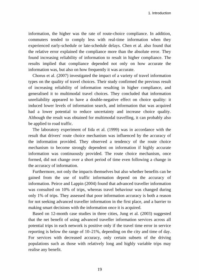
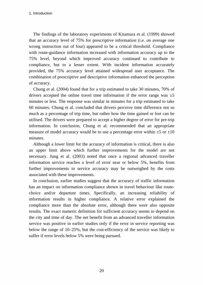
Road users benefit more from accurate travel time information where there is great variability in travel times (Jung et al. 2002). Hence, road users expect information to be up to date if the actual travel time varies substantially. Travel time information based directly on the sum of the latest measured travel times is always outdated (Figure 1), and the longer the section is, the more outdated the information. This is because by definition a vehicle has to drive the whole section before its travel time can be determined. Thus vehicles used for measuring travel time are different from those whose drivers receive information at the start of the road section based on those particular measurements (Figure 2). Without short-term prediction, accurate real-time information on travel time cannot be given.

0

10

20

30

40

50

60

13:00 14:00 15:00 16:00 17:00 18:00

Trav

el ti

me

(min

)

Target travel time Sum of latest measurements on sub-links

Figure 1. Travel time information based directly on the sum of the latest measured travel times on 9-10 km long sub-links vs. target travel time of the whole 28 km road section that was to be estimated with the sum.

1. Introduction

22

Travel timefor links AC

and BC

AB C D

Travel timefor links AD,BD and CD

Travel timefor link AB

Camera positionTravel TimeInformation

Figure 2. Vehicle whose driver sees the travel time information (on a VMS in this example), and vehicles on whose travel time the information is based. The travel time of a section is determined as the difference between the passing times at two camera stations.

Much research has been done over the past 15 years in the field of travel time prediction. Many studies are based on simulated, faultless data, which leads to well-performing models (Yasui et al. 1995, Suzuki et al. 2000, Chen and Chien 2001, van Lint et al. 2002, Nanthawichit et al. 2003). However, these models cannot cope equally well with imperfect, real-life data. Real-life applications should be robust with respect to faulty and incomplete input (van Lint et al. 2002).

Automatic travel time monitoring systems are not common, and although the whole road network cannot be covered completely with loop detectors, the traffic information collected by inductive loops or other spot-based methods is used as input for many models that predict travel time (Saito and Watanabe 1995, Lee and Choi 1998, Matsui and Fujita 1998, D’Angelo et al. 1999, Paterson and Rose 1999, Kwon et al. 2000, van Lint 2003, Zhang and Rice 2003). Even though the general relations between travel time and traffic volume, occupancy and point speed have been widely explored, these relations might not apply during saturated flow conditions (Chien and Kuchipudi 2002). However, in those conditions the travel time information is most valuable.

Studies in which travel time forecasts are based on abundant field measurements of highway travel time are few. Chien and Kuchipudi (2002) predicted travel time with a Kalman filtering algorithm, and Park and Rilett

1. Introduction

23

(1998), Park et al. (1999) and Rilett and Park (2001) predicted it with neural networks based on travel time data provided by an automatic vehicle identification system on an urban motorway. To our knowledge, the current literature does not include prediction models based on field measurements of travel times made for two-lane (1+1 lanes) two-way highways.

Few travel time prediction models that operate in an online environment have been published. The European DACCORD project included demonstrations of real-time short-term travel time prediction models that used inductive loop detectors (van Grol et al. 1999a, van Grol et al. 1999b, Lindveld et al. 2000). Three methods were tested on three fully equipped inter-urban motorway sections. The authors assessed that the accuracy of the travel time forecasts depended on the traffic characteristics. In an area with relatively stable traffic conditions, a fairly simple method might be used. The results showed that online travel time estimation using inductive loops produced RMSEPs (root mean squared error proportional) between 10% and 15% of cases up to moderate congestion levels. However, the online methods required a substantial effort to deal with the operational performance of the monitoring systems. The authors concluded that the travel time predictors either seemed to be insufficiently stable for use in a production environment, or showed great instability but could not be properly tested due to a lack of congestion at the test site.

Another real time application has been a model that made short-term travel time forecasts for a motorway section in Florida and presented them in real time on a website (Ishak and Al-Deek 2002, Al-Deek 2003). The model used a non-linear time series approach based on traffic information from densely spaced inductive loop detectors. A majority of observations produced a maximum of 10% errors, while the overall mean error and standard error of the estimates were 0.01 and 6.16% respectively. The errors ranged from –0.25 to +0.50 in minutes per mile. The results showed that the performance of the model deteriorated rapidly as congestion increased, causing errors as high as 25% to 30% under heavily congested conditions.

Both the DACCORD and Florida applications were designed for motorway sections with high-quality monitoring (i.e. detectors located every half- kilometre or half-mile, real-time data collection) using inductive loop detectors. All studies involving abundant field measurements of highway travel time conducted on motorways are based on offline models.

Interurban two-lane two-way highways with relatively small capacity and at-grade junctions differ from motorways and are more sensitive to the impacts of

1. Introduction

24

incidents. Consequently, the results obtained from motorways cannot be generalised to two-lane highways as such. However, two-lane highways are important because they carry most of the traffic in most countries. Thus, there is a lack of knowledge in the field of predicting travel time on interurban two-lane highways based on real-time field measurements of travel time.

1.4.2 Dynamic models

One impediment to the efficient use of all models mentioned in Chapter 1.4.1 is that they are static. In other words, they cannot adjust even to small systematic changes in the traffic process but require new, manmade calibration and new data. In addition, there is often too little time to collect training data, which leads to a small number of samples that represent random incidents and consequently poor ability to predict their consequences. The ability to learn while working online could improve this aspect. Hence, although such static models are practical to run online (for example no need to collect databases), they need to be based on large amounts of readily-collected varying data, and to be updated manually every now and then. A model capable of adjusting itself would be practical for long-term online use.

Ohba et al. (2000) developed a travel time prediction model based on pattern recognition. The principle of the model was that all unusual travel time observations were removed. These observations included extremely short travel times, extremely long travel times and data deviating somewhat from the travel time distribution. A typical actual travel time was calculated as the average of the remaining data. Ohba et al. chose similar patterns according to the smallest sums of the squared error. The time zone that represented 1 hour before and after the prediction moment was selected from the patterns. The most similar of these samples was chosen. The final forecast was obtained by arranging the data on the basis of the time at which the vehicles passed through an entrance toll gate.

The travel time prediction model of Otokita and Hashiba (1998) applied pattern recognition as well. They suggested that the prediction of near future was possible by the periodicity of chaotic time series data and that the traffic conditions resulting from our social activities were chaotic. In their model, traffic conditions (flow data) similar to the present were sought from a database. Samples most similar to the present traffic condition and of the time nearest to the prediction time were selected. The travel time forecast was based on the data

1. Introduction

25

from these nearest neighbours. A multiple regression model was applied to the data to make the forecast.

The models of Bajwa et al. (2003 and 2005) were also based on the assumption that the traffic scenarios similar to the present traffic condition may have occurred before. In their earlier study (Bajwa et al. 2003), the present traffic pattern was defined using occupancy measurements for 1 hour before the present time. In their later study (Bajwa et al. 2005), the time window for the pattern was adaptive to capture the effect that congestion has on travel time. Both studies used weighted patterns for defining traffic situations. A database of historical traffic situations was stored for searching the closest matched patterns with minimum squared difference.

All the models referred to above are based on the principle that in order to learn and develop, the model should constantly add new samples to the database of traffic situation samples. If all the samples are stored, the database grows fast and requires a powerful computer to run it online in real time. If only those samples that differ from the samples in the database are stored, the database becomes skewed.

Chung (2003) went about the problem by collecting the data into a database divided into segments according to the time (a.m. and p.m.), weekday, holidays and rainfall. However, it does not remove the underlying problem of ever-growing databases, although segmentation does reduce the required computer time compared with the non-segmented solution.

The larger the road network covered with prediction models, and the more input variables there are (i.e. the more diverse the monitoring system), the larger the database is and the faster it grows. Although computers are getting ever more powerful, it would be practical to find a solution other than collection of these databases.

Alecsandru and Ishak (2004) presented a hybrid model for the morning peak period of a motorway segment in Florida. They assessed that the memory-based approach (case-based reasoning) would be more efficient for predicting recurrent traffic conditions because of its memory-like structure. However, they made the assumption that a model-based predictor would be better able to capture knowledge related to non-recurrent traffic conditions. The case-based reasoning system was simply a collection of cases representing typical situations and possible solutions. If similar cases could not be found, the solution was revised and retained as a new case. In those cases, the forecast was produced with a

1. Introduction

26

neural network. The results showed that the integrated approach led to better prediction capabilities than separate approaches alone.

The approach of Alecsandru and Ishak (2004) is interesting. However, as very similar traffic situations can lead to very different outcomes, a condensed version of the history of traffic situations that they used may become either skewed (more abnormal than normal traffic situations) or not that condensed at all if the whole distribution of outcomes is presented in the database. The latter leads to the challenge of an ever-growing database. Another challenge in their approach is how to make a neural network model for non-recurrent traffic situations. That would require a database of such samples.

Kosonen et al. (2004) used a different approach. They designed a DigiTraffic concept, which pools different sources of information into an overall dynamic traffic simulation model. This model can be also used to produce short-term forecasts. The forecasting is based on the current traffic situation. A copy of that is run with maximum speed to make a near-future (15–60 minutes ahead of the present time) image of traffic. The model relies on estimates and predictions of incoming traffic volumes in the near future. The fact that these estimates and predictions are not always accurate causes ambivalence between the predicted traffic status and the real one. Ambivalence may also be caused by incidents that cannot be foreseen with the model, and the traffic-light control which may change its principles in reality within the prediction period.

The DigiTraffic concept of Kosonen et al. (2004) seems promising. However, it is a future approach to prediction making – at least on a large scale. Although computational power is probably no longer a limiting factor, traffic system dynamics are not known in enough detail to produce realistic large-scale traffic flows further into the future. In addition, the traffic monitoring network that can be used by an online application needs further development.

1.5 Effects of the monitoring system structure

Few studies discuss the effects of the structure of the monitoring system, that is, which part of the information is more important and which is less so to the prediction of the traffic situation. Usually everything available is used – which is understandable – but there is no evaluation or consideration of the additional benefit of each piece of information. Some aspects related to the structure of the monitoring system are discussed by Chen and Chien (2001), Chien and

1. Introduction

27

Kuchipudi (2002), and Park and Rilett (1998). These studies evaluate the effect of the location and of the number of detectors.

Chen and Chien (2001) studied the additional value of dividing the section into sub-links by comparing section-based travel time prediction with sub-link-based methods. In the sub-link-based method, the travel time of the section was the sum of travel times of all consisting links. Chen and Chien predicted motorway travel time with a Kalman filter based on simulated travel time data of probe vehicles. Their results showed that the section-based prediction method performed better over the sub-link-based method under normal flow conditions. They assessed that the difference in the prediction performance could be attributed to the variance of the probe vehicles. Adding link travel times together propagated the variance of the total travel time of the section. Hence, with larger variance of travel time estimates, the sub-link-based prediction models were more likely to produce less satisfactory results. However, Chen and Chien acknowledged that the simulation study could concern only recurrent, incident-free traffic conditions and that the sub-link-based method could be more sensitive to incidents than the section-based method. They assessed that intuitively, when vehicle probes are the only source of traffic data, closely tracking link travel time could facilitate incident detection.

Furthermore, Chien and Kuchipudi (2002) performed a corresponding study but applied the method to real-world data. Section-based travel time was a better pick in the morning peak hours and only while using historical data. However, throughout the rest of the day, the sub-link-based model performed relatively well. They considered that section-based travel time was reliable only when uniform traffic conditions were prevailing throughout the network, which was not always the case in real-world situations. Congestion or an incident on a sub-link did affect the value of section travel time, but when using sub-link-based models it would have affected only the travel time of that particular sub-link.

Park and Rilett (1998) indicated that intuitively, in addition to average travel times in preceding time periods, other important parameters for predicting travel time were link travel times experienced on the upstream and downstream links during the preceding time periods. They assessed that a shockwave formed upstream or downstream from the target link has the potential to affect the target link in the future. The hypothesis was certified when predicting three to five 5-minute time steps ahead in a later study (Park and Rilett 1999). In that case, the neural network model that employed travel times from upstream and

1. Introduction

28

downstream links in addition to the target link gave superior results compared to the model that only considered previous time steps from the target links.

In conclusion, in real-world application, dividing the section for which travel time needs to be predicted into sub-links is beneficial. In addition to average travel times of the target section, other important input parameters are link travel times experienced on the upstream and downstream links during the preceding time periods.

1.6 Synthesis of the literature review

Drivers can benefit from static and dynamic information of traffic situations on alternative routes by making more informed travel decisions, thus being able to improve their time management with ensuing reductions in cost and stress. Information on travel time reliability is an important factor in addition to the travel time itself. Nevertheless, the impact that information provision has on route choice, for example, also depends on other things like familiarity and complexity of the recommended route. The compliance of driver information varies with gender, standard of living and driving experience.

The provision of advanced driver information can have positive impacts on a transportation network level. Specifically, advanced traveller information can reduce congestion in transportation networks or even slightly reduce the number of injury accidents. However, traffic information may also have negative impacts if the driver cannot deal with all the information available or the provider of information does not predict, or take into account, the response of drivers to the information. In the future, cooperative information systems could help.

The value of information depends on the situation the user is in and on what kind of problem the information is supposed to solve. Information is more valuable when it is used to solve a problematic rather than normal situation. The type and length of the journey, the route and travel mode chosen, and traffic conditions all affect the value of information.

The accuracy of information is a critical factor. An aberration in system performance will not turn away users but consistent poor information will. The accuracy of the given traffic information has been shown to affect the route-choice compliance and departure times. The more reliable the information, the higher is the rate of compliance. Results have also implied that compliance depends not only on how accurate the information is, but also on how frequently

1. Introduction

29

it is accurate. There is a certain limit for error below which the information does not benefit drivers, and it depends on the location and time of day. However, there is also an upper limit above which it is not worth improving the accuracy.

Road users will benefit more from accurate travel time information where there is great variability in travel times. Hence, road users expect information to be up to date if the actual travel time varies substantially. However, without short-term prediction, real-time information on travel time cannot be given. Much research has been done over the past 15 years in the field of travel time prediction. At any rate, there is a lack of knowledge in the field of predicting travel time on interurban two-lane highways based on real-time field measurements of travel time. However, static models cannot adjust themselves but occasionally require new, man-made calibration and new data. Unfortunately, there is often too little time to collect data for creating such a model, leading to a small number of samples that represent random incidents and consequently poor ability to predict their consequences. The ability to learn while working online could improve this. Consequently, there is a lack of knowledge on how to develop a practical, self-adapting prediction model.

1.7 Purpose and hypotheses of the study

The principal aim of this study was to develop a method for making a short-term prediction model of traffic flow status (i.e. travel time and a five-step travel-speed-based classification) and to test it in a real world environment. Specifically, the objective was to find a method that could predict the traffic flow status on a satisfactory level, could be implemented without long delays, and would be practical for online use also in the long term. The main approach to the dissertation was from the viewpoint of transportation engineering. Therefore the focus was on the two-lane traffic environment, data collection, how the models were run, and on the challenges of running an online model in a real-world environment.

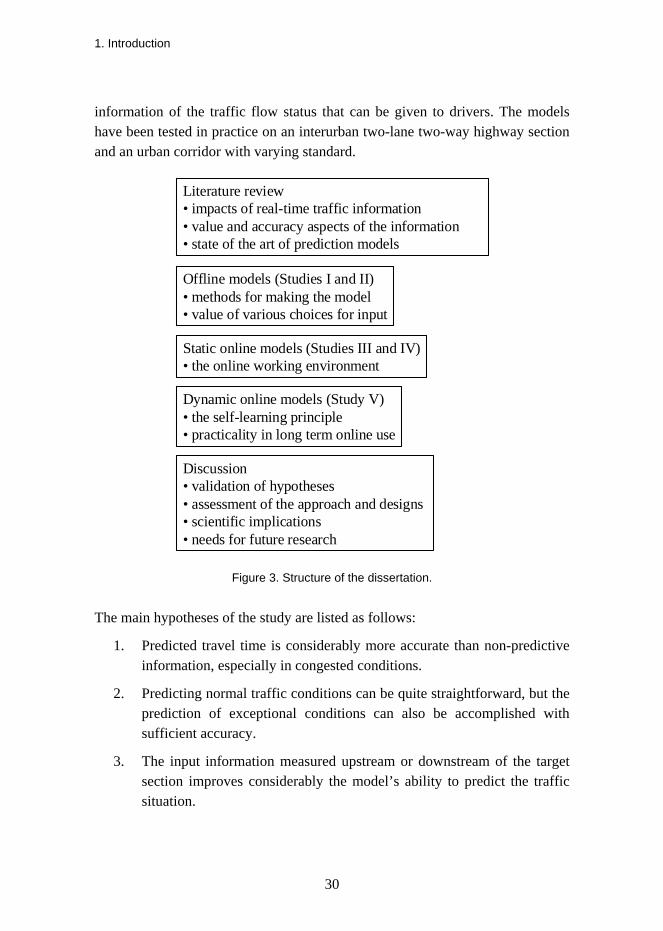
The previous chapters emphasised the impacts of real-time traffic information, the value and accuracy aspects of the information, and the state of the art of prediction models (Figure 3). The studies that form the content of the dissertation deal with the modelling of traffic flow status for short-term prediction. The sequence of articles appended shows the development process from offline models that use perfect data to online models that deal directly with field-measured data. The purpose of the online model is to produce real-time

1. Introduction

30

information of the traffic flow status that can be given to drivers. The models have been tested in practice on an interurban two-lane two-way highway section and an urban corridor with varying standard.

Offline models (Studies I and II)• methods for making the model• value of various choices for input

Static online models (Studies III and IV)• the online working environment

Literature review• impacts of real-time traffic information• value and accuracy aspects of the information• state of the art of prediction models

Dynamic online models (Study V)• the self-learning principle• practicality in long term online use

Discussion• validation of hypotheses• assessment of the approach and designs• scientific implications• needs for future research

Figure 3. Structure of the dissertation.

The main hypotheses of the study are listed as follows:

1. Predicted travel time is considerably more accurate than non-predictive information, especially in congested conditions.

2. Predicting normal traffic conditions can be quite straightforward, but the prediction of exceptional conditions can also be accomplished with sufficient accuracy.

3. The input information measured upstream or downstream of the target section improves considerably the model’s ability to predict the traffic situation.

1. Introduction

31

4. The inclusion of weather and weekday (working day vs. weekend) information improves forecasts considerably.

5. It is possible to develop a good prediction model capable of learning while working online.

In the following the general method is described, then the findings along with study-specific methods are presented in integrated form in three sections. First, the performance of a static prediction model is tested in an offline environment along with the effects of the structure of the monitoring system on forecasts (Studies I and II). Second, the same principles are applied to an online environment (Studies III and IV). Third, the principles are developed for a dynamic model that is capable of learning while working online (Study V). The model development includes improvements assessed to be necessary with respect to long-term online use and the lessons learned with the previous online model. Finally, the overall findings are discussed and recommendations given.

2. Method

32

2. Method

2.1 Data

Real-life field data was chosen as the basis for the study. As the modelling procedure was aiming at an online prediction model that works in a real world environment, all phases of the modelling – including offline models – were based on field data. Field-measured data gave robustness to the models. In comparison with simulation programs, the field data provides the realistic element of randomness missing from simulated data.

There was no information available on the incidents at the study sites during the data collection periods. Mark and Sadek (2004) showed that the addition of accident information (i.e. capacity reduction, accident location and time remaining until the accident is removed) would have improved the ability of neural networks to predict travel time in the presence of accidents.

A specific problem arises if the training data set (i.e. data that can be used for model making) does not represent the actual traffic in a comprehensive manner and includes unrepresentative samples. Such samples are often included in field-measured travel time data. There are two sources of such incorrect travel times: faults in the measurement system itself, and the measurement of travel times that are unrepresentative4 for information. All these false observations should be identified and excluded from the input data in order to get a realistic picture of the traffic situation. When making an offline model, the data can be filtered partly manually. However, for online use, the filtering procedure has to be automatic.

4 Unrepresentative travel times are unrepresentative in the sense that we do not attempt

to predict travel times of drivers who have stopped on the section to make e.g. a phone call, or temporarily diverted from the section and then returned.

2. Method

33

In a measurement system based on reading licence plates, the automatic pattern recognition process is not fully accurate and may cause mismatches, which lead to incorrect interpretations of the travel time. Deviating observations also exist, as there are always some samples of vehicles that have not travelled the route for which the travel time is actually measured. This is because some vehicles stop along the section or turn off it and come back if the detector net excludes minor intersections. In addition, there may be some vehicles that have travelled the route without obeying the legislation (e.g. a motorcycle passing slow queues along the hard shoulder or centre of the road) and thus represent irrelevant travel times with regard to the traffic being predicted.

Partial manual checking of the data employing graphical printouts was chosen when making the offline model (Studies I and II) because of the sensitivity of the educated human eye. It is hard to replace it with a simple algorithm without losing some valid data. Because the number of observations measured in congested conditions was limited, it was in our interests to use as much of it as possible. Therefore an objective and rigorous alarm system (the moving average) was set to identify data periods that might experience some problems, but as congestion sometimes develops quickly, they may also be samples of a true fast-increasing congestion. The educated human eye was used in a systematic way to resolve which case was which.

On the other hand, the monitoring system on the site of static models was new when the offline study started, and at that time we were still hoping that the problems leading to e.g. small sample size could be resolved before a real online application was ready. Hence, it was desirable to carry out the study without limiting it to the present problems.

2.2 Prediction models

Feedforward multilayer perceptron (MLP) neural networks (Studies I–IV) and self-organising maps (SOM, Study V) were chosen for this study. They are described separately for each model in the relevant chapters and Appendix B. The choice of method was made in each case without further investigation. Several methods have been used successfully in prediction models as described in the previous chapter, and any one of them could have been chosen. However, neural networks had previously been successfully proven to be useful in prediction of traffic flow status by the author (Innamaa and Pursula 2000 etc.).

2. Method

34

In addition, neural networks were an established technique in solving non-linear problems with no theoretical solution available.

2.3 Evaluation of the effectiveness of the model

The order of superiority of the models depended on which measure of effectiveness was used. Road users want information to be sufficiently accurate as often as possible, regardless of whether the model makes slight errors. Consequently, when making prediction models for travel time, the effectiveness of the models was determined as the proportion of forecasts that lay within an accepted error margin. The width of the 10% accepted error margin was used in this study. It is in accordance with the limit of 13% set by Toppen and Wunderlich (2003) or the limits of 10% to 21% obtained by Jung et al. (2003).

2.4 Procedure

A self-adapting online model was developed as follows: First, an offline model was developed (Study I), during which the methods for making the model and the value of various choices for input were evaluated (Studies I and II). In an offline environment, many challenges related to working in the real world – such as delays in data transfer or faults in the monitoring equipment – either do not exist or can be excluded. The second step was to study how the online working environment affected the model and how those effects should be taken into account (Studies III and IV). Challenges related to the online working environment included delays and online filtering of data. Finally, it was investigated how the model should be if it is run online in the long term. At that stage the self-adapting feature was added to the model (Study V).

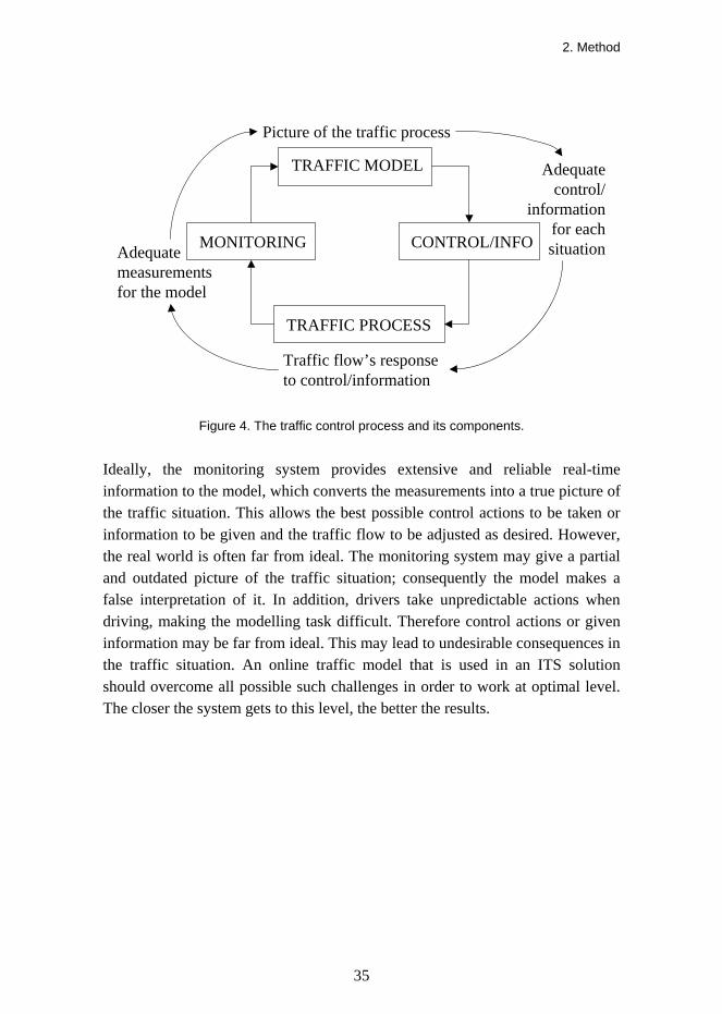
The traffic model is one of four elements of the traffic control process consisting of the model, traffic control or information, the traffic process and the monitoring system (Figure 4). Traffic control or information affects the traffic flow. Its effects can be seen using the monitoring system. The traffic model interprets the measurements and updates the traffic situation picture, which in turn forms the basis for adequate control of information.

2. Method

35

MONITORING CONTROL/INFO

TRAFFIC MODEL

TRAFFIC PROCESS

Traffic flow’s responseto control/information

Adequatemeasurementsfor the model

Picture of the traffic process

Adequatecontrol/

informationfor eachsituation

Figure 4. The traffic control process and its components.

Ideally, the monitoring system provides extensive and reliable real-time information to the model, which converts the measurements into a true picture of the traffic situation. This allows the best possible control actions to be taken or information to be given and the traffic flow to be adjusted as desired. However, the real world is often far from ideal. The monitoring system may give a partial and outdated picture of the traffic situation; consequently the model makes a false interpretation of it. In addition, drivers take unpredictable actions when driving, making the modelling task difficult. Therefore control actions or given information may be far from ideal. This may lead to undesirable consequences in the traffic situation. An online traffic model that is used in an ITS solution should overcome all possible such challenges in order to work at optimal level. The closer the system gets to this level, the better the results.

3. Offline model for travel time prediction (Studies I and II)

36

3. Offline model for travel time prediction (Studies I and II)

3.1 Purpose of the offline model study

The purpose of the offline model study was first to investigate the predictability of travel time with a model based on travel time data measured in the field on an interurban two-lane two-way highway (Study I). Second, the purpose was to determine whether the forecasts would be accurate enough to implement the model in an actual travel time information service (Study I). Specifically, a target was set to get 90% of the forecasts within a 10% error margin (±10%). In practice, this 10% accepted error was approximately 2 minutes in free-flowing traffic and up to 5 or 6 minutes in congestion for the whole study section. Finally, the purpose was to investigate how the structure of the measurement system affected the short-term forecasts of travel time based on it (Study II). Specifically, the effects of section length and the location of different measurement stations were investigated.

3.2 Method

3.2.1 Study site

Studies I–III were carried out on Finnish main road 4 between the cities of Lahti and Heinola in southern Finland. The study section was an interurban two-lane two-way highway section with alternating passing lanes. Because the site was located between two motorways, traffic congestion was a problem during weekend peak hours with the heaviest traffic. The free-flow travel speed on the section was around 100 km/h. In congested conditions the travel time might be up to three times normal – especially northbound on Fridays. The average

3. Offline model for travel time prediction (Studies I and II)

37

summer traffic volume on the section (both directions together) was 17,000 vehicles per day and the traffic volume exceeded 2,000 vehicles/hour during the busiest hours (Finnra 2001). The proportion of heavy traffic was on average 13% and during workdays 20%.

The 28 km long study section was equipped with an automatic travel time monitoring system. The system was based on an image processing and neural network application, which automatically reads licence plates at several locations in both directions (Finnra 2000).

There were two types of monitoring stations within or near the study site: camera stations belonging to the travel time monitoring system, and inductive loop detectors. The study section was divided into three sub-links by four camera stations (marked A, B, C, and D in Figure 5). The distance between two consecutive camera stations varied between 8.7 and 10.3 km. Inductive loop detectors were installed at location C and 11.9 km south of location A on the other side of the nearby city to gather information about traffic volumes and point speeds. Loop detectors north of the study section could not be used in the offline model studies (Studies I and II) due to a monitoring station malfunction.

Camerastation

Camerastation

Inductiveloop detectors

Inductiveloop detectors

Lahti

Heinola

9.1

km

8.7 km10.3 km

11.9 km

A

B

CD 9.1 km

Figure 5. Study site with number of lanes, link lengths and traffic monitoring equipment. The section contained four camera stations (A–D) used to measure travel time, and inductive loop detectors at location C. There were also loop detectors south of A and north of D, on the far side of the cities closest to the section.

3. Offline model for travel time prediction (Studies I and II)

38

According to the data, in the southbound direction DA congestion always occurred between camera stations D and C. In the opposite direction, AD, congestion occurred most often between camera stations B and C and sometimes also between camera stations A and B. When there was congestion on sub-link AB it usually meant that the congestion on sub-link BC was more severe than when traffic on sub-link AB was flowing freely. Congestion on sub-link BC did not always indicate problems on sub-link AB, as the traffic on AB could also be flowing freely despite congestion on BC. The cause of the congestion was unknown. In the direction DA, traffic on sub-link CA and in the opposite direction on sub-link CD was always flowing freely.

VMSs located 4.2 km south of location A and 1.5 km north of location D displayed expected travel times between the two cities for northbound and southbound travellers, respectively. The goal of the system was to inform drivers about congestion and to offer an estimate of the expected travel time. The underlying rationale was that congestion is more tolerable when drivers are aware of the expected traffic conditions, as shown by Luoma (1998). In addition, travel time information was provided on the Internet.

In the original system of the Finnish Road Administration, the travel time displayed on VMSs was not a forecast but an estimate of travel time. This was based on the sum of latest measured travel times for each sub-link – or on a combination of sub-links in case one or two camera stations were not operating along the section. The range of travel time shown on VMS was based on 25% and 75% points of travel time observations. However, the minimum difference between the lower and upper limit of the shown travel time information was set to be 5 minutes and the minimum lower limit was set according to speed limits. In conditions where the mean travel speed was lower than 75% of the free flow speed (i.e. congested conditions), the VMS in the northbound direction displayed the correct travel time information (measured value was between the upper and lower limit shown on the VMS) 32.9% of the time and in the opposite direction 49.7% of the time.

3.2.2 Data

Studies I and II were based on data collected over roughly 4 months in summertime conditions 24 hours a day, 7 days a week. The raw data of individual vehicles produced by the travel time monitoring system as well as inductive loops near the study site were included. The travel time monitoring

3. Offline model for travel time prediction (Studies I and II)

39

system was capable of reading on average 40% of all licence plates on the monitored lane at a single point in good conditions when the camera was clean. The travel time measurement system was installed only for one lane per direction. Consequently, only the northbound traffic flow at camera stations B and C was fully monitored, as camera stations A and D were located on motorways (2+2 lanes) and at locations B and C the southbound direction had two lanes. Hence, the sample sizes were small in the travel time monitoring system and the number of travel time observations was not equal to the flow. The monitoring system did not keep a record of the types of passed vehicles (heavy vs. light).

Most of the data was from free-flowing traffic. Traffic was defined as congested if the mean travel speed was lower than 75% of the free-flow speed, i.e. slow, queuing or stopped traffic, according to Kiljunen and Summala (1996) in Table 1.

Table 1. Definition of flow status classes. These definitions are based on the driver’s perception of the traffic situation (Kiljunen and Summala 1996).

Flow status Travel speed / free speed (%) Free-flowing traffic > 90 Heavy traffic 75–90 Slow traffic 25–75 Queuing traffic 10–25 Stopped traffic < 10

An objective and rigorous alarm system (the moving average) was set to identify questionable periods of individual vehicle travel-time data. However, as congestion sometimes develops fast, these could also be samples of a true quickly increasing congestion. An educated visual evaluation was made to determine which it was, minimising the unnecessary loss of data as the number of observations measured in congested conditions was limited.

After filtering, the data was aggregated. This data included 1-minute average and median travel times, and the median travel time and standard deviation of the observations from the last 5 minutes or the last 10 or 20 vehicles. In addition, it included the 1-minute flow, mean point speed and standard deviation of the point speed at the inductive loop detectors.

3. Offline model for travel time prediction (Studies I and II)

40

3.2.3 Prediction models

The offline models (Studies I and II) were made as feedforward MLP neural networks to keep the model simple but effective. A separate neural network was trained to predict the travel time of each sub-link. As output, the models gave the average travel time for vehicles entering the section within the following minute. The 1-minute aggregation period was chosen to ensure fast detection of the changes in travel times. The drawback of the 1-minute average is that it is less stable and more sensitive to erroneous observations than e.g. a 5-minute average; the advantage, however, is that it detects tendencies or changes faster. The sample sizes would also have been greater for a longer aggregation period, but as this model was made for study purposes to run offline and the raw data could be checked manually, the problems caused by small sample size were partly overcome.

The input traffic information obtained by the models was based on the latest measurements of traffic volumes and point speeds, in addition to the latest travel time information (measured for vehicles having exited the link during the time period in question.). The input parameters were selected according to their correlation with the travel time to be predicted (referred to hereafter as the prediction travel time) and to the mutual correlation of the input parameter candidates.

The time series of average travel times was chosen as the basis for input of the prediction models. The criterion of a minimum correlation coefficient of 0.20 with the prediction travel time was used for testing input parameters. However, if two input parameter candidates had a high mutual correlation (minimum coefficient of 0.95), the parameter that correlated most highly with the prediction travel time was chosen and the other parameter was excluded from the input. Several lengths were used for the input time series: five, four and three consecutive 1-minute observations. The selected input parameters are given in Appendix B.

The raw data did not include observations for each sub-link for every minute. The input data set was built on the principle that the value of an input parameter was assumed to be invariant until a new observation was obtained. However, if the information on some of the input parameters was older than 30 min, the sample was dropped from the training set. All samples without a fresh measurement for the output parameter were excluded from the set.

3. Offline model for travel time prediction (Studies I and II)

41

The number of input neurons was equal to the number of input parameters; the number of output neurons was one, since there was just one output parameter (Appendix B). The input parameters were normalised to have a zero mean and standard deviation of one. The structure of the neural network was to be kept simple: neural networks were to have one hidden layer. The number of hidden neurons was such that the number of training samples was at least ten times the number of parameters to be estimated. However, the number of hidden neurons was limited to no more than 20 to keep the training process fast. The activation function of the hidden layer was chosen to be a hyperbolic tangent and that of the output layer a linear function.

Neural networks were trained with the Fletcher–Reeves update (Demuth and Beale 2001), which is one of the conjugate gradient algorithms. In this study, several stopping conditions were given to prevent the neural network from learning the training data too well. These criteria were the maximum number of training epochs, the minimum values of the gradient and of the mean squared error, and the point at which the mean squared error of the calibration data stopped decreasing. In practice, training stopped most of the time because of the latter. For this latter criterion, the original training data set was divided into three sub-sets: training, calibration and validation set. The training was performed with the training set. The calibration set was used to track the point at which the model started to learn the peculiarities of the training set and no longer the general features of the modelled phenomenon. The validation set was not used in the training process in any way. It was used, however, after the training to check how the model performed with new data.

3.3 Results

3.3.1 Statistical examination

The statistical examination was performed with different error terms: the mean error and relative error, the mean absolute value of error and relative error, and the mean squared error (Study I). The first two error terms measured whether the model tended to underestimate or overestimate the travel time; the last three measured the magnitude of the errors.

The length of the time series of input travel time information was chosen for each model so as to minimise the error terms. The results showed that the models were very good at prediction over all time periods (mean squared error

3. Offline model for travel time prediction (Studies I and II)

42

0.2–2.5 min2 and mean error 0.0 for all sections) and that the majority of the forecasts were close to the measured values (mean relative error 0.5–0.7% and mean absolute value of relative error 5.5–6.9%). However, on average the models tended to slightly overestimate the forecasts rather than underestimate them.

In practice, most of the forecasts that were considered false were outcomes of situations where the models predicted travel time to be less than 20 min but the measured travel time was 22–25 min (i.e. slightly outside the accepted 10% error margin). On section DA, all these observations were from situations where the model missed an isolated longer travel time (an isolated peak). Besides missing isolated peaks, the model for section AD was also occasionally delayed from the start of congestion.

Isolated peaks were either local, quickly-resolved incidents or situations where filtering of the raw data had been too coarse. After filtering, some observations remained for which it was hard to tell whether they were deviant. If the mean value is based on a few observations only, an individual deviating observation may have a significant effect on it.

The first type of error (missing a short isolated peak) was not serious – or could even be considered beneficial – but errors of the second type (being delayed from the start of congestion) should be avoided. However, it is challenging if the first signs of an unusual situation cannot be measured until after making the forecast. In that case it is hard to come up with an analysis technique that could resolve the problem of being delayed from the start of congestion.

3.3.2 Effectiveness in terms of the information system

The VMS informed road users that the travel time would be the predicted travel time ±10% (i.e. the accepted error margin was chosen to be ±10%). However, the absolute minimum travel times shown would be those based on the speed limit; i.e. predicted travel times shorter than those would not have been shown. Hence, the displayed travel time was not considered erroneous if vehicles travelled faster than the limit and the VMS showed the minimum travel times allowed.

First, the correctness of the forecasts was investigated for both uncongested and congested traffic together (Study I). The same analysis was also made for samples for which the average travel speed was less than 75% of the free flow speed (congested conditions). These proportions could not be defined for all the

3. Offline model for travel time prediction (Studies I and II)

43

sub-links, because they had almost no congestion whatsoever during the data collection period.

All the models in direction DA gave correct travel time information more than 97% of the time on average, and in the opposite direction more than 95% of the time. If the forecasts for sections AD and DA had been presented on VMSs in congested conditions, the proportion of correct forecasts would have been 71% of the time for section AD and 79% for section DA.

A limited examination was performed on the width of the accepted error margin. An increasing number of forecasts lay within the margins, as the margins were set further away from the 0% error, but this increase got smaller as the margins became wider. When the width of the accepted margin was changed from 5.0% to 7.5% the proportion of correct forecasts improved by 15.4 percentage points on average, whereas the improvement was 11.6 percentage points when the width was changed from 7.5% to 10.0% and 8.6 percentage points if it was changed from 10.0% to 12.5%, being only 5.8 percentage points when the width was changed from 12.5% to 15.0%.

3.3.3 Effects of the monitoring system structure

The effects of the structure of the measurement system were studied (Study II) based on the available detectors at the test site (four camera stations and two inductive loop detectors). The study was conducted by assuming that only part of the measurement equipment would be available. Hence, the models were always made to predict the travel time solely on the basis of input parameters measured by the detectors in use in each particular case.

First, it was assumed that the travel time information system was based only on the two camera stations at the start and end of the section for which the travel time was predicted. For all sections starting from the same point, the proportion of correct forecasts in congested conditions increased with the length of section.

Second, the impact of additional camera stations on the forecast was studied, as well as where they should be located. Additional camera stations increased the proportion of correct forecasts in congested conditions compared with the models based on two camera stations only. The more additional camera stations there were, the bigger the proportion was. The improvement with one well-located additional camera was up to 14 percentage points and with two additional cameras up to 21 percentage points. An additional camera station within or upstream of the section improved the results more than a station

3. Offline model for travel time prediction (Studies I and II)

44

downstream of it. This difference was up to 7 percentage points and 4 percentage points, respectively. It also seemed that an additional camera close to the starting point of the section improved the results more than an additional station close to the end point. The difference was up to 10 percentage points.

Finally, the effect of information obtained from inductive loop detectors on the results was studied. The information from the loop detectors did not improve the results as much as the information from additional camera stations. However, the effect of additional loop information was also favourable. Specifically, the improvement was up to 8 percentage points compared with the model with no loop information. The loop detector station south of location A improved the results more than the detector at location C, the difference being up to 5 percentage points. The two loop detector stations together improved the results more than just one detector did, this improvement being up to 10 percentage points.

3.4 Discussion

This offline model study was designed, first, to investigate the predictability of travel time when the forecast was based on travel time data measured in the field on an interurban two-lane two-way highway (Study I). Second, the purpose was to determine whether the forecasts would be accurate enough to implement the model in an actual travel time information service (Study I). Finally, this study was designed to investigate how the structure of the measurement system affected the forecasts (Study II).

In conclusion, the results of the offline travel time prediction model were found to be promising, and even this kind of simple prediction model could improve the accuracy of travel time information, especially in congested conditions (Study I). The findings suggested that forecasts could be improved by setting up an adequate monitoring system (Study II).

The structure of the monitoring system was shown to affect the forecasts (Study II). Additional camera stations and inductive loop detectors could offer information that improved the model’s ability to react to changes in a traffic situation. The main findings of Study II suggested that the structure of the monitoring system should be based on an analysis of congestion. It was important to know where congestion usually occurs in the area and how it develops. Besides the two cameras that measure travel time along the whole section, it was important to minimise the data collection delay in the area where congestion usually developed. For better accuracy as to the timing of the start of

3. Offline model for travel time prediction (Studies I and II)

45

congestion, the prediction model should include information on incoming flow rates. A travel time monitoring system does not have to be equally distributed along the section for which the travel time is predicted. It is important to cover the area well where congestion usually builds up; the rest of the section can be left with less inspection. On that part of the section, the distance between two consecutive cameras should be based on the maximum delay for detecting incidents.

4. Static online model for travel time prediction (Studies III and IV)

46

4. Static online model for travel time prediction (Studies III and IV)

4.1 Purpose of the static online model study

The purpose of the static online model study (Studies III and IV) was to test the lessons learned with the offline prediction model presented in Chapter 3, and bring the model to the online real-world environment. First, the performance of the online prediction model was evaluated on the basis of a trial period (Study III). Second, the potential to improve the model in situations where its performance was not satisfactory was examined (Study III). Finally, the purpose was to discuss the challenges posed by working in real time in a real-world environment (Study IV).

4.2 Method

4.2.1 Study site

The research on the static online model (Studies III and IV) was conducted on the same site as the offline model study (Studies I and II, Figure 5). However, the loop detectors north of location D on the far side of the nearest city (outside the section) that could not be used in the offline model study (Studies I and II) were used in the static online model study (Studies III and IV).

4.2.2 Data

The prediction model of the pilot study (Study III) was based on approximately 4 months of summertime data (training phase data). Night-time observations (22:00–08:00) were excluded due to the low amount of traffic. The travel time data was the raw data produced by the monitoring system. Deviating individual

4. Static online model for travel time prediction (Studies III and IV)

47

travel time observations in the raw data were not excluded in real time because the number of observations per aggregation period was not sufficient to judge which observations were true and which were biased.

The prediction model had to overcome all the delays caused by the online working environment. The model received data every 5 minutes. The collection of travel time data caused a delay equal to the travel time itself, whereas the data transfer produced no significant additional delays. However, the aggregated loop information was usually received with a 10 to 15 minute delay.

The travel time prediction model was run online. This study used data from a 14-month-long period (evaluation phase data). The travel time estimates based directly on the latest measurements (the original non-predictive system) were collected for comparison over the same time period.

A VMS was installed on the study section at the start of the pilot trial period (evaluation phase) to provide information in congested conditions about an alternative route on a parallel road. This information led to more vehicles choosing the alternative route than before the sign was installed, and probably slightly changed the shape of the congestion.

4.2.3 Prediction models

The prediction models were constructed as MLP feedforward neural networks (Studies III and IV). The main principles behind the structure of the neural networks were based on the offline models (Study I). The numbers of neurons in different layers are shown in Appendix B.

Travel time was predicted for the northbound and southbound sections AD and DA (Study III). As output, the prediction model gave the expected median travel times for vehicles entering the sections within the next 5 minutes, while the last measurements were used as input.

Travel times on sub-links that were never congested during the data collection period were excluded from the input data set (Appendix B), because they had poor correlation with the travel time to be predicted (less than 0.2 in congested traffic). At any rate, the travel time of the always free-flowing links (a constant) would make no difference as input because the neural network has to learn to vary the prediction travel time along with the changes in the input travel times that vary. Therefore only the variables with higher correlation coefficients were selected for the input. The input data consisted of the three latest values of each input quantity. In the training procedure, no data transfer delay was used for the

4. Static online model for travel time prediction (Studies III and IV)

48

travel time data, whereas the delay was assumed to be 10 minutes for point-based information.

As individual vehicle travel time data could not be filtered online, individual median values were assessed before accepting them. If the median was based on the travel time of a single vehicle, the value was updated only if the new value differed from the old value by less than 20%.

Some situations arose where part of the input was unknown. However, it was considered worthwhile to make predictions even then. Hence, a separate neural network was created for each detector combination, simulating situations where one or several detectors were out of order. If the information break from an individual detector lasted 30 minutes or less, the input value was kept unchanged until a new value was received. If the break was longer than 30 minutes, the forecast was made using a neural network that was trained without that particular piece of information.

The travel time was not predicted if too many or critical detectors were down (Appendix B), because it was crucial for the credibility of the system that overly unreliable forecasts were not shown. The neural networks that produced forecasts that were correct less than 60% of the time in congested conditions during the training phase were left out. Consequently, there were 10 neural networks predicting travel time for the northbound section AD, and 13 neural networks for the southbound section DA.

4.3 Results

4.3.1 Evaluation results of the online model

Not all the neural networks made to predict travel time with different detector combinations were used during the trial period (evaluation phase, Study III). Specifically, there were three models in the northbound direction AD and five models in the opposite direction that were used for more than 3 hours in congested conditions. All these models gave correct forecasts 94–99% of the time on average. Specifically, the longest northbound link AD gave correct forecasts 97% of the time and the opposite direction link DA gave them 99% of the time. In congested conditions, the proportion of correct forecasts varied between 34% and 80% of the time, the models of the longest links AD and DA producing correct forecasts 53% and 80% of time.

4. Static online model for travel time prediction (Studies III and IV)

49

The prediction model performed worse in the online environment (evaluation phase) than expected on the basis of the training phase results. However, the prediction model still performed much better than the original non-predictive system.

A detailed analysis of the development of congestion and the corresponding performance of the prediction model showed that the model was able to predict the travel time for the southbound section DA when sub-link DC was congested. When the input information from the inductive loop detector north of location D was missing, the shape of the predicted congestion was correct but the forecast came 10–15 minutes late. When the input information from the inductive loop detector north of location D was missing, and the camera station at location C was down, the forecast came 20–30 minutes late and the peak of the congestion was not always at the correct level. No forecasts were made with all the detectors working. The model did not detect congestion on other sub-links caused by incidents and predicted free-flowing traffic.

The performance of the southbound model DA could be considered satisfactory, although it was not as good as expected. At least part of the decline in performance could be explained by inactive detectors and random incidents creating congestion different from the instances of congestion in the training set.

The northbound model AD did not predict the travel time well in all circumstances. Congestion on the northbound section AD was a more diverse phenomenon than in the opposite direction. Hence, the reasons for unsatisfactory performance of the model were less evident than those of the southbound model DA. In the northbound direction AD, congestion was more severe than in the opposite direction, thus the effect of route guidance information in the form of travel time information displays (VMS) might also have been greater. It was unclear whether the model was sufficiently complex to process the congestion phenomenon in the northbound direction AD or whether the phenomenon itself changed due to the route guidance information.

The findings suggest that the southbound model DA could be accepted as such, while the northbound model AD should be improved. Despite partially unsatisfactory results, the prediction model still performed much better than the original non-predictive system, which gave travel time estimates based on the latest measurements.

4. Static online model for travel time prediction (Studies III and IV)

50

4.3.2 Further development of the model

The objective was to improve the prediction performance of the northbound model AD, because either the model was not sufficiently complex to process the congestion phenomenon or the phenomenon itself changed due to the route guidance information (Study III). The method used to further develop the model was the same as before except for (1) a new data set, (2) additional input for the models, and (3) the number of hidden neurons. The new data set (evaluation phase data) represented the new traffic situation, while the last two items increased the complexity of the model.

First, a similar model as in the original pilot version of the prediction model was made using data collected during the trial period (evaluation phase data). Second, the benefit of increasing the number of input variables was examined. Third, the effect of an increase in the number of hidden neurons was studied. Finally, new neural networks were made for all the detector combinations, with the improvements found to be beneficial.

A similar neural network as in the first pilot version of the prediction model was made using the data collected during the pilot trial period. The ability of the model to predict correct travel times in congested conditions improved substantially over the model trained with original training phase data. The proportion of correct forecasts increased from 53% to 64%. The overall performance improved in producing correct forecasts from 97% to 98% of the time. Consequently, the use of the new data set was beneficial.

The effect of the additional input information in the form of new variables (the travel time of road section CD, the mean speed at location C and the traffic volume at the loop detector south of location A, on the far side of the nearby city) was beneficial, but small. The complexity of the model was increased both by adding new input variables and by increasing the number of hidden neurons from 20 to 30, 40 and 50. The performance of the model improved slightly as the number of hidden neurons was increased.

4.3.3 Challenges specific to the online environment

Often monitoring systems are not originally designed for the purposes of the online traffic model. Challenges in the monitoring system are related to data supply delays, incorrectly working detectors and other failures (Study IV). Problems related to these challenges may lead to a false picture of the traffic

4. Static online model for travel time prediction (Studies III and IV)

51

situation, no matter how good the traffic model is. A false interpretation of the traffic situation may result in incorrect control actions or information, which have a negative impact on traffic flow.

Data supply delays have to be considered when constructing a model. The delay may be due to data collection or data transfer. If individual vehicle data is stored and transmitted forward by the monitoring system in aggregated form, data processing also takes time and causes delay. In many cases, the cost of data transfer varies according to the frequency with which the data is transferred. If the monitoring system is designed mainly for the compilation of statistics, the frequency is probably kept low. Thus if the model is to predict several minutes ahead of the present moment, in reality it has to be able to predict that plus the delay in receiving the information.

A detector may break down and stop functioning. In addition to long breaks, in our experience there are many short, less than 30-minute-long breaks in data supply for one reason or another. Failures in communication systems such as a mobile phone network or Internet connections cause breaks in data transfer as well. Hence, although the monitoring system might be working well, there could be temporary problems with data transfer.

The lack of synchronisation between different clocks in the measurement system may cause errors in the data. Usually the challenge is to detect clocks that are gradually losing or gaining time. Initially the lapse is small, but over time the error increases.

An online telematics application relies on the interpretation of the traffic situation that it receives from the traffic model. However, the model may interpret the traffic situation erroneously if the traffic model cannot deal with the data it receives from the monitoring system, if the model receives incorrect information or if it is used beyond its scope. False interpretations may lead to incorrect control actions or information and thereby to undesirable consequences.

A model that works properly in an offline environment may encounter problems in an online environment. The change from simulated data to real-world data may lead to problems if the model is not robust enough, because online field data may include greater variation than simulated data. Even if the offline model is based on field data, problems may arise when only a relatively small amount of field data is used in developing the model.

Even if the training data of the model is representative and covers all normal situations, it can never cover all possible incidents. A great variety of incident

4. Static online model for travel time prediction (Studies III and IV)

52

scenarios should be considered when designing the model. The creation of different incidents is easy with a simulation model, but the response of the model to incidents should be of special concern when working with field data. Consequently, the scope for which the model is calibrated should always be acknowledged and the model should be used beyond it only with caution.

A specific problem arises if the training data set includes false or irrelevant observations. All of them should be identified and excluded from the input data to get a realistic picture of the traffic situation.

The sample may also be biased and unrepresentative of the actual traffic flow. At the site of Studies I–III, the travel time monitoring system did not cover the overtaking lane, which alternated from one direction to another. The basic lane gave an idea of the fluency of traffic flow on the road, but the sample of vehicles that were detected by the system did not represent a random sample of the whole traffic flow. Therefore it should be acknowledged that the traffic picture produced by the model, and on which the displayed information was based, was biased.

It is important to understand the deficiencies of detectors and the limitations that they pose in the model. For example, camera detectors are sensitive to dirt, snow and glare. Hence, their detection rate is seldom as high as it would be in permanently good circumstances. Because of the low detection rate, the number of traffic measurements that can be used in the model is limited. For this reason it is good to use median values, which are likely to be less sensitive to a small sample than mean values or standard deviations.

Loop detectors do not always function faultlessly either. They may miss certain types of vehicles (e.g. motorcycles) or vehicles driving on the edge of the lane, or they may detect vehicles driving in the adjacent lane. Long or wide loops are problematic since two vehicles can occupy them at the same time, which may corrupt the vehicle count.

4.4 Discussion

This study was designed to present a static online prediction model that predicted travel times on an interurban two-lane two-way highway section on the basis of field measurements of the travel time and point-based quantities. The study was in three parts. First, the performance of the pilot version of the prediction model was evaluated on the basis of the trial period (Study III). Second, the possibility of improving the model in case its performance was

4. Static online model for travel time prediction (Studies III and IV)

53

unsatisfactory was examined (Study III). Finally, experience was gathered to provide guidelines to assist those developing online traffic situation models (Study IV).

The main implication of the studies presented so far was that even a simple prediction model making short-term travel time forecasts using neural networks can improve the accuracy of travel time information substantially compared with an estimate based directly on the latest measurements (Study III). The results of further development of the model showed that its performance, which had not been on a satisfactory level, could be improved especially with new data containing more instances of congestion. The remaining problem with the prediction model was that if the congestion phenomenon changed for whatever reason, the model would need to be retrained. Furthermore, the model cannot learn random incidents. Hence, the development of a self-adjusting or self-adapting model is important. With online operation there is limited time for the collection of training data, and therefore the system should basically learn from its own mistakes and try to perform better next time.

As many of the challenges related to the online working environment cannot be avoided, models should be developed to be robust, and they should regard all incoming data with suspicion (Study IV). In addition, the model should accommodate information that is incomplete in one way or another. Model developers should also understand the weaknesses that may result from biased data. If the traffic picture received by a model developer does not correspond fully to reality, the output of the model – no matter how close to the measured values – will also not correspond to reality as the driver sees it.

5. Dynamic online model for flow status prediction (Study V)

54

5. Dynamic online model for flow status prediction (Study V)

5.1 Purpose of the dynamic online model study

The purpose of the dynamic online model study was to develop a method for making a self-adapting short-term prediction model for the flow status (i.e. the five-step travel-speed-based classification of Kiljunen and Summala (1996), Table 1 on page 39). Specifically, the objective was to find a method that (1) could predict the flow status on a satisfactory level, (2) would learn by itself during online operation, and (3) would also be practical for long-term online use. The method was to be tested in the Helsinki metropolitan area.

5.2 Method

5.2.1 Self-organising maps

A SOM (Kohonen 2001) is, in its basic form, an unsupervised neural network method that can be used when the classification of the data is unknown or the use of this classification is unwanted. The approach can also be called cluster analysis, clustering, or profiling of data. A SOM consists of neurons (processing units or map units) organised on a regular low-dimensional grid. Distances between the map units can be measured with the distance of their weight vectors in grid coordinates.

The weight vectors connect each map unit with a counterpart in the pattern space and accordingly each pattern vector (input vector of the model) with the map unit whose weight vector is closest to the pattern vector. The distribution of weight vectors tends to follow the distribution of the training data. Therefore the map can be used to generalise data when the number of map units is small. In

5. Dynamic online model for flow status prediction (Study V)

55

pattern recognition, similar vectors tend to locate to map units that are close to each other on the grid. Consequently, similar samples are located close to each other.

A SOM is trained iteratively. The best matching map unit (BMU) and its topological neighbours on the map are moved according to the samples in the training set. Supervised learning proceeds in the same way as the unsupervised basic method. However, the class information is added to the patterns in the training phase. Consequently, the separation of classes is better when compared to unsupervised learning.

5.2.2 Study site

The study site was Ring Road I in the Helsinki metropolitan area. The road was regularly congested during morning and evening peak hours on working days (Monday to Friday, Figure 6). The annual average daily traffic volume was up to 85,000 vehicles and the highest daily traffic volumes exceeded 100,000 vehicles on the busiest working days. The traffic volume exceeded 9,600 vehicles per hour for the busiest 100 hours of the year in the middle part of the road (3+3 lanes), being around 6,000 vehicles per hour in the western and eastern parts of the road (2+2 lanes). The speed limit ranged from 60 km/h to 80 km/h.

The test road started in the west with 2+2 lanes. The number of lanes was 3+3 from the Otaniemi junction to main road 110 and from main road 120 to main road 45 (Figure 6). The road had an alternating bus lane in addition to the 2+2 lanes east from main road 4. The westernmost part of the road was connected to the street network by signal-controlled at-grade intersections, and only the main roads (marked on the map in Figure 6) were connected by grade-separated intersections. From main road 120 to main road 4, connections to the test road were only with grade-separated intersections. In the easternmost part, the street and road network was connected by signal-controlled at-grade intersections, except for the road to Mellunkylä, which connected via a grade-separated intersection.

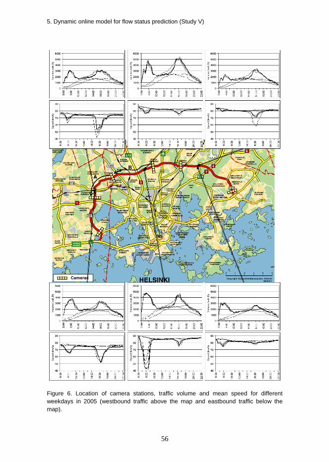
5. Dynamic online model for flow status prediction (Study V)

56

Figure 6. Location of camera stations, traffic volume and mean speed for different weekdays in 2005 (westbound traffic above the map and eastbound traffic below the map).

5. Dynamic online model for flow status prediction (Study V)

57

Six camera stations (Figure 6) were used for automatic travel time monitoring on the test road. Cameras divided the road into 3.1–7.4 km-long sections. The results of the study were analysed for the two most congested road sections (A and B, Figure 6). Section A was from the third to the second camera station from the west; section B was from the fourth to the third. On section A there were on average 67.3 minutes of successful measurements of congestion per day and, respectively, 39.6 minutes per day on section B. Traffic flow was determined to be congested if the average travel speed was under 75% of the free flow speed. On all other sections of the test road, the average amount of successful measurements of congested traffic was less than 20 minutes per day.

5.2.3 Data

Raw travel time data collected by the travel time monitoring system were used in the study. Models were based on data collected during an 8-month period from January to August 2004. The prediction performance of the models was tested during a 250-day period starting in January 2005.

The raw travel time data were aggregated into median values of 5-minute periods. These data were filtered to avoid individual deviating observations over-affecting the median values. Several filtering methods were evaluated. This was done by checking visually which observations were filtered and which were not. Specifically, the researcher plotted the observations that were filtered and those that were left on the computer screen. An educated human eye was able to judge the performance of the automatic filtering procedure. As the filtering had to be performed online and its performance was critical, especially when the number of observations was small, a simple method based on two threshold values seemed to work better than more sophisticated methods of using polynomial fitting. In the chosen filtering method, if the number of observations was less than three, the maximum difference from the latest accepted median was allowed to be 50%. Otherwise, the median was rejected.

In addition to the travel time data, it was also possible in the prediction procedure to use the information on weather and road conditions from a measurement point near the test road on the intersecting main road 3. The weather and road conditions were classified into three categories: normal, poor and hazardous.

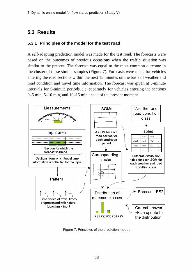
5. Dynamic online model for flow status prediction (Study V)

58

5.3 Results

5.3.1 Principles of the model for the test road

A self-adapting prediction model was made for the test road. The forecasts were based on the outcomes of previous occasions when the traffic situation was similar to the present. The forecast was equal to the most common outcome in the cluster of these similar samples (Figure 7). Forecasts were made for vehicles entering the road sections within the next 15 minutes on the basis of weather and road condition and travel time information. The forecast was given at 5-minute intervals for 5-minute periods, i.e. separately for vehicles entering the sections 0–5 min, 5–10 min, and 10–15 min ahead of the present moment.

Figure 7. Principles of the prediction model.

5. Dynamic online model for flow status prediction (Study V)

59

The outcome of the model was defined as the traffic flow status class of the road section in question. The outcome of the traffic situation was described with five traffic flow status classes determined from the ratio of measured travel speed to free speed (Table 1 on page 39). Traffic flow was considered congested if the flow status class was slow, queuing or stopped.

The model input included a time series of the three latest measurements of 5-minute median travel times of the preceding road section, the road section in question, and the following road section. The input was pre-processed before making the SOM so that none of the input variables dominated over the others, i.e. long travel times over shorter ones. The natural logarithm separated travel times better than scaling or normalising and was therefore applied to the values.

For making the prediction model, the similarity of traffic situations (i.e. pattern vectors) needed to be determined and then clustered in a systematic way. Any method could have been chosen as long as it did not require original pattern vectors to be kept in a database. One solution for clustering was the SOM. SOMs along with the outcome distribution tables formed the prediction model.

To make the model learn while working online from the traffic situations it encountered, the distribution of outcome classes was updated in the cluster used for making the forecast as soon as the “correct” answer was measured in the field. Consequently, there was no need to restore the samples to a database; rather, all that was needed was to increase the number of matches in an outcome distribution table. This table was as big as the number of clusters times the number of outcome classes. Updating of the flow status outcome tables was performed at 5-minute intervals. If for some reason no observations were measured, the tables were left untouched.

5.3.2 SOM for the model

A separate SOM was made for each road section and for each of three prediction periods, based on the principles of supervised learning using a hexagonal map grid lattice (Appendix B). A sheet shape was selected for the map topology. The desired number of map units (Munits) was determined with the heuristic formula of Vesanto et al. (2000), where dlen was the number of samples in the training data.

Munits = 20 · dlen0.54321

5. Dynamic online model for flow status prediction (Study V)

60

The final map size was determined by calculating the two biggest eigenvalues of the training data and by setting the ratio of the side lengths equal to the ratio of these values. The final side lengths were set so that their product was as close to the desired number of map units as possible.

During training, a SOM was formed to present typical observations. In practice, the proportion of important cases (here, congestion) in the training set was small. Consequently, these cases might not be able to gain any ground of their own from the map. Therefore, the training data were collected by randomly selecting an equal number of 4,000 samples from each flow status class. This led to SOMs that had from 2,196 to 2,822 map units (Appendix B).

5.3.3 Sub-models

A trial was carried out on the effect of weather and road conditions on forecasts. Forecasts were made without weather and road condition information; it was then studied whether the performance of the model differed in different weather and road conditions. The results showed that the average performance of the model was similar for both normal and hazardous weather and road conditions. However, some differences were observed when the results were analysed by flow status class. Specifically, free-flowing traffic was predicted less accurately when the weather and road condition was hazardous than when it was normal. For other flow status classes, the situation was the opposite. When the weather and road condition class was poor, the performance of the model was similar to that for normal weather and road condition status, the result being between the performances for normal and hazardous.

The model was divided into sub-models according to the weather and road condition class (normal, poor, hazardous), although poor or hazardous conditions were rare on the test road because of the high flow rate and good maintenance in wintertime. On a road section the same SOM was used for all weather and road condition classes for the same prediction period, but the flow status outcomes were collected into separate tables based on weather and road conditions.

The effect of day of the week was investigated similarly to that of weather and road conditions. During weekends the proportion of free-flowing traffic was notable (95.9–100.0%, being above 99.0% on seven of the ten road sections). Because the free-flowing weekend traffic was predicted on average with more success than during the week, there was no need to integrate information on the

5. Dynamic online model for flow status prediction (Study V)

61

day of the week into the model. Most of the very few, solitary observations of congested weekend traffic were not predicted correctly.

5.3.4 Practicality in long-term use

The practicality of the model in long-term online use can be assessed from e.g. the number of carry bits it takes to restore the history of traffic situation samples. In long-term use, the model should be able to run for several years if no significant changes are made to the road network. In 5 years this would lead to a database of 63,072,000 items (34,560 items per day) if all the history were stored for a site with 10 road sections, and nine inputs and three outputs to store per road section. By comparison, the dynamic online model presented in this study stores a condensed version of the same history in ten tables of fixed size not exceeding 14,110 items.

5.3.5 Online trial

An online trial was conducted on the test road. The input information received from the field was aggregated, filtered and pre-processed with a natural logarithm (Figure 7). The Euclidian distance from the input to each map unit of SOM (presented as a matrix of weight vectors of map units) was calculated. The map unit with the shortest distance was selected as the BMU. The forecast was determined as the most common flow status outcome of that particular map unit and weather and road condition class. Finally, when (if) the correct answer was measured in the field, the corresponding outcome distribution table was updated for the corresponding map unit and weather and road condition class.

The model was allowed to work online and its performance was studied as a function of time for a 250-day period. The proportion of correct forecasts was 93.8% over the entire trial period and 80.9% in congested conditions for the model of road section A in normal weather and road conditions. Corresponding proportions were 96.3% and 82.3% for the road section B.

As expected, workdays had an influence on forecasts. Weekend (Saturday-Sunday) traffic was mostly free-flowing and those forecasts succeeded better than the ones made during the week (during weekends, road section A: 96.8%, road section B: 99.6% vs. during the week, road section A: 92.5%, road section B: 94.9%). According to Student's t-test, the difference in performance between workdays and weekends was statistically significant for both road sections (road

5. Dynamic online model for flow status prediction (Study V)

62

section A: p = 0.001, road section B: p = 0.000). During congestion the proportion of correct forecasts on workdays was 83.2% for road section A and 84.2% for road section B. At weekends there were very few, solitary observations of congested traffic on both road sections, and for the most part these were predicted wrongly.

It was hypothesized that the performance of the model improves with time, as it is able to adapt itself. The average daily change in the proportion of correct forecasts was indeed positive over the whole trial period: +0.4% for road section A and +0.3% for road section B. Student's t-test was used to determine whether this difference was statistically significant. The equality of variances was tested with Levene's test. The performance of the first 30 days of the trial was compared with that of the last 30 days. The test showed that the difference in performance was statistically significant for the model of road section A (p = 0.000) but not for that of road section B (p = 0.089).

Two naïve comparison models were made. The first one based the forecast on average travel time for the 5-minute period and day of the week in question for each road section. These average values were calculated from the same 2004 data used to make the model. The second comparison model used the latest measurements directly as forecasts. Both models were tested over the same trial period in 2005 as above. The latest measurements (83.2% for all conditions, 53.1% for congestion) performed better on road section A than the averages (83.7% for all conditions, 1.7% for congestion). On road section B the reverse was true (averages: 89.7% for all conditions, 49.6% for congestion; latest measurements: 88.6% for all conditions, 40.5% for congestion). Both comparison models performed considerably worse than the self-adapting model.

5.4 Discussion

This study was designed to develop a method for making a self-adapting short-term prediction model for the traffic flow status. The objective was to develop a method that could predict the flow status on a satisfactory level, would learn by itself during online operation, and would also be practical for long-term online use. The method was tested in the Helsinki metropolitan area.

As a result of the study, principles accordant with the objectives were developed for a self-adapting model and for prediction of the flow status. Specifically, the structure of the model (clustering and updating of the outcome tables) made it possible for the model to learn by itself without the need to save

5. Dynamic online model for flow status prediction (Study V)

63

all the data. The performance of the model could be considered satisfactory in relation to the coarseness of the monitoring system. The results also indicated that the self-adapting principle improved the performance of the model. Naïve models performed far worse than the self-adapting model.

The model does not react fast to changes in traffic patterns, i.e. to situations where a certain traffic pattern starts to lead to a different outcome than previously. Hence, if there are considerable changes in the road network or traffic management (e.g. new signal timing at an entry to the motorway), it is better to initialise the outcome tables and start the collection of historic information anew. Slow changes like annual growth in traffic volumes change the most commonly used map units, but as the outcome is the same as previously with the same traffic volumes, there is no need to initialise the tables for that reason. However, if a major change (e.g. structural improvement of the road) is made, it is best to collect a new training data set and create new SOMs and outcome distribution tables for the model.

In conclusion, if the flow status outcome classes are well separated into clusters, a model based on the principles described in this chapter should be able to detect even the impacts of incidents on flow status increasingly well over time. Also of importance is that there is no need to save all the data into databases, which makes long-term online use practical in terms of the number of carry bits it takes to restore the history of samples of traffic situations.

6. General discussion

64

6. General discussion

6.1 Validation of hypotheses

The principal aim of this study was to develop a method for making a short-term prediction model of traffic flow status (i.e. travel time and a five-step travel-speed-based classification). Specifically, the objective was to find a method that could predict the traffic flow status to a satisfactory level, could be implemented without long delays, and would be practical for online use also in the long term. The main hypotheses of the study were: (1) predicted travel time is considerably more accurate than non-predictive information, especially in congested conditions; (2) predicting normal traffic conditions can be quite straightforward, but the prediction of exceptional conditions can also be accomplished with sufficient accuracy; (3) the input information measured upstream or downstream of the target section improves considerably the model’s ability to predict the traffic situation; (4) the inclusion of weather and weekday (working day vs. weekend) information improves forecasts considerably; and (5) it is possible to develop a good prediction model capable of learning while working online.

As expected in the first hypothesis, predicted travel time is on average considerably more accurate than non-predictive information, especially in congested conditions. The hypothesis was confirmed, as the results of the static prediction models (Studies I and III) indicated that even a simple prediction model could improve substantially the accuracy of travel time information, especially in congested conditions. In congested conditions, the original non-predictive travel time information was correct 31% of the time in the northbound direction, while the offline model (Study I) would have produced correct travel times 73% of the time and the improved online model (Study III) 64% of time. In the opposite direction, the corresponding proportions would have been 47% for the non-predictive information, 83% for the offline model and 80% for the

6. General discussion

65

online model. The findings of the offline model study suggested that the forecasts could be improved by setting up an adequate monitoring system for the specific site.

According to the second hypothesis, predicting normal traffic conditions can be quite straightforward, but the prediction of exceptional conditions can also be accomplished with sufficient accuracy. At the study site of the static prediction models (Studies I–III), traffic was exceptionally congested over many summer weekends; however, the shape and timing of the congestion varied. The rest of the time, traffic could be considered normal. Over the whole study period, the average proportion of correct forecasts of the (improved) online model was 98% in the northbound direction and 99% southbound (Study III). As these figures include both normal and exceptionally congested conditions, the corresponding proportions being 64% and 80% in congested conditions, it suggests that normal traffic conditions can be predicted to a high degree and the first part of the second hypothesis is correct.

There were several samples of exceptional traffic congestion during summertime weekends at the test site of the static prediction models (Study III). The definition of sufficient accuracy can, of course, be argued. Nevertheless, if the prediction model doubles the proportion of correct travel time information over the original non-predictive information, the accomplishment can be considered sufficient, although the target limit of providing correct information about exceptional conditions more than 75% of time set by Kitamura et al. (1999) could not be attained for all the links. A contrary example is from the study site of the dynamic model, where there were very few, solitary observations of congested traffic during weekends (Study V). Most of them were not predicted correctly. That implies that the more samples of exceptional traffic congestion there are, the better is the ability of the model to predict them. Therefore, the latter part of the second hypothesis is probably correct only if there are a sufficient number of samples of these exceptional conditions. In the modelling attempts within this study, however, the second hypothesis was not fully verified.

The third hypothesis suggested that the input information measured upstream or downstream of the target section improves considerably the model’s ability to predict traffic situations. Regarding the effects of the monitoring system’s structure on the performance of the offline prediction model, the results showed that an additional camera station within or upstream of the section improved the results more than a station downstream of it (Study II). The

6. General discussion

66

difference was up to 7 percentage points and 4 percentage points, respectively. Consequently, although congestion did not always build up from one sub-link to another but was spatially limited at that study site, upstream information turned out to be important; even if it did not help to time the start or end of the congestion, it helped to evaluate the level to which the travel time increased.

Travel time information indicating congestion in the upstream section was important to the model of the downstream section; however, this did not appear to hold in the opposite direction – at least at that particular study site of static models (Studies I–III). If there was congestion upstream it usually meant high traffic demand and the congestion downstream was more severe than if the traffic upstream was flowing freely. Because part of the upstream congestion was caused by incidents that reduced the upstream capacity, upstream congestion did not always indicate problems on the downstream section; in fact traffic on the downstream section could be flowing freely. Hence, the small additional value of the extra downstream cameras was justifiable (Study II).

Detailed analysis showed that the static online model was able to predict the travel time for the southbound section DA when the first of three sub-links was congested (Study III). The shape of the predicted congestion was correct, but the forecast came 10–15 minutes late when the input information from the inductive loop detector upstream of the section was missing. The delay was equal to that in receiving the first signs of a change in traffic situation. These findings suggest that the information about incoming flows is very important for the correct timing of congestion.

Based on these results, the third hypothesis could be verified only for the upstream information. The findings suggest that the structure of the monitoring system or the area from which the input information is collected for the prediction should be based on an analysis of congestion (Study II). The collection area should be wider than the target section; however, the question of widening it upstream or downstream should be dependent on this analysis.

According to the fourth hypothesis, the inclusion of weather and weekday (working day vs. weekend) information improves forecasts considerably. The effect of the weather and road surface condition information on forecasts was investigated for the dynamic model (Study V). The results showed that the average performance of the model was similar both for normal and hazardous weather and road surface conditions. However, there were some differences in the results when they were analysed by flow status classes. Specifically, free-flowing traffic was predicted less accurately when the weather and road surface

6. General discussion

67

condition was hazardous than when it was normal. For other flow status classes, the situation was the opposite. These results indicate that the separation of weather and road surface condition classes is beneficial. Consequently, the inclusion of weather information improves forecasts. However, as poor and hazardous weather and road surface conditions are rare on a road like the test road because of the high flow rate and good winter maintenance, the effect on the average performance of the model is modest – although it would probably be significant when these conditions occur more frequently.

Weekend traffic was mostly free flowing at the dynamic model study site (Study V). Specifically, the flow was free-flowing 96–100% of the time during weekends, being above 99% on seven of the ten road sections. On average, weekend forecasts succeeded statistically significantly better than during the week. However, during congestion, the proportion of correct forecasts was on a satisfactory level during workdays and the very few, solitary observations of congested weekend traffic were usually predicted incorrectly. However, as explained previously, the more seldom and probably more random the congestion, the more difficult it is to predict. As the proportion of weekend congestion was so small, even considerable improvement in the ability to predict it would not have influenced the average numbers significantly. In addition, as the probable main cause for the weekend congestion is incidents, one could ask whether a considerable improvement in the ability of the model to predict their consequences can be achieved. Therefore the latter part of the fourth hypothesis is not verified – at least for sites with practically no weekend congestion.

Finally, as was assumed in the fifth hypothesis, it was possible to develop a good prediction model that is capable of learning while working online. The results of the dynamic online model indicated that the self-adapting principle improved the performance of the model over time (Study V). Specifically, the average daily change in the proportion of correct forecasts was positive over the whole trial period: +0.4% and +0.3% for the studied road sections. This difference was statistically significant for both road sections. The results showed that the difference in the performance of the first and last 30 days of the trial was statistically significant for one of the two studied road sections while being marginally not significant for the other (p = 0.089). Naïve comparison models performed considerably worse than the self-adapting model. As the overall performance of the self-adapting model was good (proportion of correct forecasts 93.8% and 96.3% over the entire trial period and 80.9% and 82.3% in congested conditions, Study V), the fifth hypothesis was verified.

6. General discussion

68

6.2 Assessment of the approach and designs

The sequence of articles shows the development process from offline models that use perfect data (Studies I and II) to online models that deal directly with field measured data (Studies III–V). Although a dynamic self-adapting online model could have been developed directly, the weaknesses and influences of various factors on the model’s performance could be analysed more systematically using a stepwise approach.

The performance of a prediction model is highly dependent on factors like the causes of congestion, location of congestion origin, amount of congested traffic, and the structure and technical performance of the detector network. Regular phenomena and free-flowing traffic are easier to predict than random incidents and severe congestion, and the prediction task is easier for a model based on densely-spaced, well-working detectors rather than on sparsely-spaced or often malfunctioning ones. Due to the application of specific circumstances, a numeric comparison between models developed for and tested at different sites is not terribly meaningful. The task of making sophisticated comparison models for the same sites using the same data as the models created in this study would have been overly laborious and was therefore omitted. However, naïve comparison models performed far worse than the self-adapting model of Study V and it can be argued that as self-adapting, the model performed better than as a static version (i.e. without the self-adapting feature), as it improved its performance considerably during the online trial.

MLP neural networks were selected to form the body of the static prediction models (Studies I–IV). Perhaps some other method could have performed equally well, but the choice of MLP was justified by the encouraging results in previous studies using it (Park and Rilett 1999; McFadden et al. 2001; Shao et al. 2002). MLP neural networks have also proven to be good in predicting other measures that describe the traffic situation like flow rate (Smith and Demetsky 1994, 1997; Lee et al. 1998; Innamaa and Pursula 2000). In addition, any method capable of clustering samples in an objective and explicit way could have been chosen for the self-adapting model (Study V). SOM was chosen because it fulfilled these requirements.

Field data were chosen as the basis for the study, as the modelling procedure was aiming at an online prediction model that works in a real-world environment. Data produced by a simulation model would have made it possible to test any kind of scheme. However, as the traffic flow produced by simulation

6. General discussion

69

programs is not fully realistic, it was decided to limit the study to scenarios available in field data produced by the current monitoring systems at the study sites. The limitations of the field data were seen most strongly in the study of the effects of the monitoring system structure (Study II). However, the results obtained by real-world data were assessed to be more valid than those produced by simulated data. Hence, less detailed but more valid results were preferred.

The effectiveness of the models was determined as the proportion of forecasts lying within an accepted error margin (Studies I–III). Hence, the width of this margin had a major effect on numeric values that measure effectiveness. The width of the accepted error used in this study was 10%. This is in accordance with the limit of 13% set by Toppen and Wunderlich (2003), or the limits of 10% to 21% obtained by Jung et al. (2003). The chosen margin width seemed to separate the performance of different models well, especially when the performance was measured in congested conditions. Consequently, the width was justified.

6.3 Scientific implications

This study generated several implications of value to science. The main ones are discussed briefly below. The main implication – especially for sites where congestion is a random rather than recurring phenomenon – is that models should be made with the self-adapting principle (Studies III–V). Online operation offers limited time and possibilities for learning; therefore the system should learn from its own mistakes and aim to perform better next time. The self-adapting principle also made it possible to implement the model quite quickly.

The structure of the dynamic model (Study V), especially the updatable condensed history in table form, was an essential contribution. A simple practical solution produced a great measurable advantage. The model was more practical for long-term online use, in terms of the number of carry bits it takes to restore the history of samples of traffic situations, than the models presented in the earlier studies as there was no need to store all the samples of the traffic situation (Study V). The models developed by Ohba et al. (2000), Otokita and Hashiba (1998) and Bajwa et al. (2003) required an ever-expanding database to be kept and used, which could in time lead to challenges in dealing with large amounts of data. For example, at the site of Study V, had all the samples been stored this would have led to a database of 63 million items in 5 years, as

6. General discussion

70

demonstrated in Chapter 5.3.4. By comparison, the condensed version of the same history was stored in ten tables of fixed size of at most 14,000 items. The difference is large, although the number of input parameters was rather small at that site, as was the number of road sections for which the forecasts were made. The same principle can be applied to much more complex systems and extensive sites. As the history has to be used online in real-time, the condensed version of the history sets fewer requirements on the computer running the model, and is therefore more practical to use.

Another main contribution was the successful online use of the models in practice in a real-world environment (Studies III and V). Specifically, a model was created for the first time for a site representing an interurban two-lane two-way highway section (Studies I–III). Another new environment for a model was the urban corridor with a relatively sparsely spaced monitoring system and varying standard (Study V). Neither of the sites had strong recurrent congestion.

The study also contributed to science in basing the models mainly on direct travel time measurements (Studies I–V), as most of the previous models that use field-measured data are based on point-based measurements. In particular, the combination of field measurements of travel times and two-lane two-way highway was modelled for the first time with considerable success (Studies I–III).

Another and major implication is that the structure of the monitoring system at a site where a prediction model is implemented should be based on an analysis of congestion (Study II). A travel time monitoring system does not have to be equally distributed along the section. It is important to cover sufficiently the area where congestion usually builds up, leaving the rest of the section with less inspection. On that part of the section, the distance between two consecutive sensors should be based on the maximum delay for detecting incidents.

Furthermore, for correct timing of the start of irregular, over-demand-caused congestion, it is important to get information about the flows entering the section and at problematic locations (bottlenecks etc.) along the section (Study III). Another important aspect for which flow information could be helpful is the evaluation of whether the measured travel times make sense. If there is no information on flow rates, it is impossible to distinguish whether long travel times are likely due to over-demand, an incident, or a failure in the measurement system. Self-evaluation of the incoming data is a crucial part of a model working online (Study IV).

6. General discussion

71

6.4 Needs for future research

Many studies have argued that the accuracy of information is crucial in relation to the benefits the information offers. However, only a few studies have defined what sufficient accuracy is; all that can be said at this point is that their results are site-dependent. However, the definition is also dependent on the driver and on the characteristics of the information system. More studies measuring the benefits and determining minimum, or rather optimum, accuracy levels for the information are needed before general conclusions can be made.

The literature review suggested that the provision of advanced driver information can have positive impacts on a transportation network level. Specifically, advanced traveller information can reduce congestion in transportation networks or even slightly reduce the number of injury accidents. However, these studies are based on telephone interviews, expert opinions and models, not field-measured real-world data. It is left for future research to prove that these effects really exist.

Another matter for future research is the online filtering of data. The model should work smoothly despite imperfect input information. In this study, a simple filtering method was chosen based on a cursory comparison (Studies III and V). Although the method seemed to work on a satisfactory level, the filtering method suitable for online models and small samples should be developed further.

The results indicated that up-to-date traffic volume information could improve traffic status forecasts. It is left for future research to develop a model based on principles developed for the dynamic prediction model with input that includes, besides the travel time information, good-quality up-to-date traffic volume information on main incoming flows and at bottleneck locations.

Simulation models should be developed further, also on two-lane roads. There is a clear demand for producing training data for prediction models with simulation. Such data could contain all kind of traffic scenarios along with a variety of incidents. However, to produce training data for an online application, the simulation model should be able to produce traffic scenarios that are realistic both macroscopically and in detail, and that cover a wide range of realistic situations. To accomplish that, traffic system dynamics should be studied further in detail, with special emphasis on incidents.

The future of traffic status prediction models may include hybrid models in which real time traffic measurements are fed to simulation-based prediction

6. General discussion

72

models. The first steps of this research have already been taken in small scale applications by Kosonen et al. (2004).

The future of traffic management includes cooperative traffic management where information can be passed selectively to road users. Such management provides new possibilities for the road operator to optimise the use and performance of the road network. However, it brings new challenges to the modelling of traffic situations, which become more dependent on the management decisions taken by the road operator. A first step in understanding the process would be predicting the effects of the travel time prediction on user behaviour and the consequent dynamic changes in the traffic flow pattern across the entire network.

The future will also bring personalised travel time prediction models that operate as a dynamic layer for navigation. This kind of solution calls for a flexible model capable of predicting the travel time between any given points within a given time window.

One more matter for future research is moving from prediction of incident impacts (e.g. on travel time) to prediction of incidents on the basis of flow pattern changes etc. As the impacts of incidents cannot be foreseen before the first signs can be measured, and even then the ability to make a correct forecast varies, it would be a significant advantage to be one step ahead and to be able to predict the incident itself.

6. General discussion

73

References Abdel-Aty, M.A., Kitamura and R., Jovanis, P.P. (1995). Investigating effect of travel time

variability on route choice using repeated measurement stated preference data. Transportation Research Record 1493, TRB, National Research Council, Washington D.C. Pp. 39–45.

Aittoniemi, E. (2007). Tieliikenteen tietopalveluiden vaikutusmahdollisuudet liikenneturval-lisuuteen (Potential safety impacts of in-vehicle information services). AINO-publications 46/2007, Ministry of Transport and Communications, Helsinki. 107 p.

Al-Deek, H. (2003). The impact of real-time and predictive traffic information on travelers’ behavior in the I-4 corridor. Final report, University of Central Florida. 117 p.

Alecsandru, C. and Ishak, S. (2004). Hybrid model-based and memory-based traffic prediction system. Transportation Research Record, No. 1879, Transportation Research Board, Washington DC. Pp. 59–70.

Bajwa, S., Chung, E. and Kuwahara, M. (2003). Travel time prediction method based on pattern matching technique. In: Proceedings of 21st ARRB and 11th REAAA Conference, Cairns, Australia. 14 p.

Bajwa, S., Chung, E. and Kuwahara, M. (2005). Performance evaluation of an adaptive travel time prediction model. In: Proceedings of the 8th International IEEE Conference on Intelligent Transportation Systems, Vienna, Austria, September 13–16, 2005. 5 p.

Ben-Akiva, M., de Palma, A. and Kaysi, I. (1991). Dynamic network models and driver information systems. Transportation Research, Part A, Volume 25A, No. 5. Pp. 251–266.

Bonsall, P. and Palmer, I. (1999). Route choice in response to variable message signs: Factors affecting compliance. In: Emmerink, R. and Nijkamp, P. (eds.). Behavioural and network impacts of driver information systems. Ashgate, Hants. Pp. 181–214.

Chen, M. and Chien, S. (2001). Dynamic motorway travel time prediction using probe vehicle data: link-based vs. path-based. Transportation Research Record 1768, Transportation Data and Information Technology. Pp. 157–61.

Chen, P., Srinivasan, K. and Mahmassani, H. (1999). Effect of information quality on compliance behavior of commuters under real-time traffic information. Transportation Research Record, No. 1676. Transportation Research Board, Washington, D.C. Pp. 53–60.

6. General discussion

74

Chien, S. and Kuchipudi, C. (2002). Dynamic travel time prediction with real-time and historical data. Transportation Research Board, Washington DC. Remarks: Paper 02–2548 prepared for presentation at the 81st annual meeting of the Transportation Research Board, Washington, D.C. 26 p.

Chorus, C., Arentze, T. and Timmermans, H. (2007). Information impact on quality of multimodal travel choices: conceptualizations and empirical analyses. Transportation, 34, pp. 625–645.

Chung, E. (2003). Classification of traffic pattern. In: Proceedings of the 10th World Congress on Intelligent Transport Systems, Madrid, Spain, 16–20 Nov. 2003. ERTICO, Brussels. 11 p.

Chung, E., Warita, H., ul Islam Bajwa, S. and Kuwahara, M. (2004). Travel time prediction: issues and benefits. In: Proceedings of 10th World Conference on Transport Research, (CD), Istanbul, Turkey. 11 p.

D’Angelo, M., Al-Deek, H. and Wang, M. (1999). Travel time prediction for motorway corridors. Transportation Research Record 1676, Travel Behavior and Passenger Travel Demand Forecasting. Pp. 184–191.

Demuth, H. and Beale, M. (2001). Neural networks toolbox for use with Matlab. User’s Guide, Version 4. The Math Works Inc. Pp. 5-1–5-75.

Emmerink, R. and Nijkamp, P. (1999). Scope of driver information systems. In: Emmerink R. and Nijkamp, P. (eds.). Behavioural and network impacts of driver information systems. Ashgate, Hants. Pp. 1–12.

ERTICO (1998). ERTICO News, January 1998, pp. 10.

Finnra (2000). Vt 4 Lahti–Heinola matka-ajan seuranta- ja informaatiojärjestelmän toiminnan arviointi (Main road 4 Lahti–Heinola journey time monitoring and information system functional analysis). Finnra Reports 58/2000. Häme District of Finnish National Road Administration, Tampere. 46 p. + app. 61 p.

Finnra (2001). Liikenteen automaattinen mittaus 2000. Tielaitoksen sisäisiä julkaisuja 25/2001, Finnish Road Administration, Helsinki. 6 p. + app. 200 p.

van Grol, H., Danech-Pajouh, M., Manfredi, S. and Whittaker, J. (1999a). DACCORD: Online travel time prediction. In: Meersman, H., van de Voorde, E. and Winkelmans, W. (Eds.) World Transport Research, Selected proceedings of the 8th World Conference on Transport Research, volume 2: Planning, operation, management and control. Pp. 455–467.

6. General discussion

75

van Grol, R., Lindveld, K., Manfredi, S. and Danech-Pajouh, M. (1999b). DACCORD: Online travel time estimation/prediction results. In: Proceedings of 6th World Congress on Intelligent Transport Systems (ITS), held Toronto, Canada, November 8–12, 1999. 12 p.

Herrala, M. (2007). The value of transport information. VTT Research Notes 2394, VTT Technical Research Centre of Finland, Espoo. 87 p. + app. 5 p. http://www.vtt.fi/inf/pdf/tiedotteet/2007/T2394.pdf

Iida, Y., Uno, N. and Yamada, T. (1999). Experimental analysis of effects of travel time information on dynamic route choice behaviour. In: Emmerink, R. and Nijkamp, P. (eds.). Behavioural and network impacts of driver information systems. Ashgate, Hants. Pp. 215–239.

Innamaa, S. and Pursula, M. (2000). Liikennemäärän ja nopeuden lyhyen aikavälin ennustaminen (Short-term prediction of flow and speed). Finnra Reports 54/2000. Finnish National Road Administration, Helsinki. 101 p. + app. 3 p.

Ishak, S. and Al-Deek, H. (2002). Performance evaluation of short-term time-series traffic prediction model. Journal of Transportation Engineering, November/December 2002, Volume 128, Number 6, pp. 490–498.

Jiang, M. and Morikawa, T. (2004). Theoretical analysis of the variation of value of travel time savings. Transportation Research Part A 38, pp. 551–571.

Jung, S., Larkin, J., Shah, V., Toppen, A., Vasudevan, M. and Wunderlich, K. (2002). On-time reliability impacts of advanced traveler information services (ATIS), Volume II: Extensions and applications of the simulated yoked study concept. Final report, Mitretek Systems, Falls Church, Virginia. 152 p. + app. 14 p.

Jung, S., Larkin, J., Shah, V., Toppen, A., Vasudevan, M. and Wunderlich, K. (2003). On-time reliability impacts of ATIS, Volume III: Implications for ATIS invesment strategies. Final report. 85 p. + app. 14 p.

Khattak, A.J., Yim, Y. and Stalker, L. (1999). Does travel information influence commuter and noncommuter behaviour? Results from the San Francisco Bay Area TravInfo project. Transportation Research Record, No. 1694. Transportation Research Board, Washington DC. Pp. 48–58.

Khattak, A.J., Youngbin, Y., Stalker and Prokopy, L. (2003). Willingness to pay for travel information. Transportation Research Part C 11, pp. 137–159.

Kiljunen, M. and Summala, H. (1996). Ruuhkaisuuden kokeminen ja liikennetilanne-tiedottaminen. Tienkäyttäjätutkimus kaksikaistaisilla teillä. (Perception of traffic

6. General discussion

76

conditions, and traffic information – a road user survey on two lane roads). Finnra Reports 25/1996, Finnish National Road Administration, Helsinki. 77 p. + app. 5 p.

Kitamura, R., Jovanis, P., Abdel-Aty, M., Vaughn, K. and Reddy, P. (1999). Impacts of pre-trip and en-route information on commuters' travel decisions: Summary of laboratory and survey-based experiments from California. In: Emmerink, R. and Nijkamp, P. (eds.). Behavioural and network impacts of driver information systems. Ashgate, Hants. Pp. 241–267.

Kohonen, T. (2001). Self-organizing maps. Third edition, Springer series in information sciences. Springer, Berlin. 501 p.

Kosonen, I., Kulmala, R. and Hautala, R. (2004). DigiTraffic – Liikenteen mallinnus- ja palvelujärjestelmä, esiselvitys (DigiTraffic – On-line traffic modelling for telematics services, Feasibility study). FITS-publications 30/2004, Ministry of Transport and Communications, Helsinki. 109 p.

Kulmala, R. (2007). Reference to discussion of Risto Kulmala, VTT, with Paul Kompfner from ERTICO 20.11.2007.

Kurauchi, F., Iida, Y. and Aizawa, T. (2000). An evaluation of effect of travel time information from real-time origin-destination matrices estimation model. In: Proceedings of the 7th World Congress on Intelligent Systems, held in Turin, Italy. 8 p.

Kurri, J. and Pursula, M. (1995). Finnish Preliminary Value of Time Studies. VTI:s och KFB:s forskardagar (The Swedish Road and Transport Research Institute and The Swedish Transport and Communications Research Board). In: Proceedings of KFB and VTI forskning/research 14-del 4. Linköping, Sweden, 10–11 January 1995. Pp. 49–70.

Kwon, J., Coifman, B. and Bickel, P. (2000). Day-to-day travel time trends and travel time prediction from loop detector data. Transportation Research Record 1717, Highway and Traffic Safety: Crash Data, Analysis Tools, and Statistical Methods. Pp. 120–129.

Laine, T. and Pesonen, H. (2002). Tiedottaminen ruuhkatilanteiden hallinnassa Traffic information in congestion management). FITS-publications, Ministry of Transport and Communications, Helsinki. 143 p.

Lee, S., Kim, D., Kim, J. and Cho, B. (1998). Comparison of models for predicting short-term travel speeds. In: Proceedings of 5th World Congress on Intelligent Trans-port Systems, Seoul, Korea. 9 p.

6. General discussion

77

Lee, Y. and Choi, C. (1998). Development of a link travel time prediction algorithm for urban expressway. In: Proceedings of 5th World Congress on Intelligent Trans-port Systems, Seoul, Korea. 8 p.

Lindveld, C., Thijs, R., Bovy, P. and van der Zijpp, N. (2000). Evaluation of online travel time estimators and predictors. Transportation Research Record 1719. Pp 45–53.

van Lint, H. (2003). Confidence intervals for real-time motorway travel time prediction. IEEE Conference on Intelligent Transportation Systems, Shanghai, China. 6 p.

van Lint, J., Hoogendoorn, S. and van Zuylen, H. (2002). Freeway travel time prediction with state-space neural networks: Modeling state-space dynamics with recurrent neural networks. Transportation Research Record 1811. Pp. 30–39.

Luoma, S. (1998). Liikenteen sujuvuus ja sen mittaaminen (Transport system efficiency and its estimation). Finnra Reports 21/1998, Finnish National Road Administration, Helsinki. 101 p. + app. 27 p.

Mahmassani, H.S. and Liu, Y.-H. (1999). Dynamics of commuting decision behaviour under advanced traveller information systems. Transport Research, Part C, Vol. 7, pp. 91–107.

Mannering, F.L., Kim, S.G., Barfield, W. and Ng, L. (1994). Statistical analysis of commuters' route, mode, and departure time flexibility. Transportation Research, Part C, Vol. 2, No. 1, pp. 35–47.

Mark, C. and Sadek, A. (2004). Learning systems for predicting experimental travel times in the presence of incidents. Insights and lessons learned. Transportation Research Record, No. 1879, Transportation Research Board, Washington DC. Pp. 51–58.

Matsui, H., Fujita, M. (1998). Travel time prediction for motorway traffic information by neural network driven fuzzy reasoning. In: Neural networks in transportation applications. Pp. 355–364.

McFadden, J., Yang, W.T. and Durrans, S. (2001). Application of artificial neural networks to predict speeds on two-lane rural highways. Transportation Research Record 1751, Geometric Design and the Effects on Traffic Operations 2001. Pp. 9–17.

Michon, J. (1985). A critical view of driver behaviour models: what do we know, what should we do? In: Evans, L. and Schwing, R. (eds.) Human behaviour and traffic safety. Plenum Press, New York. Pp. 485–520.

6. General discussion

78

Nanthawichit, C., Nakatsuji, T. and Suzuki, H. (2003). Application of probe vehicle data for real-time traffic state estimation and short-term travel time prediction on a motorway. Transportation Research Board 82nd Annual Meeting, Compendium of papers CD-ROM, Washington D.C. 16 p.

Noland, R. (1999). Information in a two-route network with recurrent and non-recurrent congestion. In: Emmerink, R. and Nijkamp, P. (eds.). Behavioural and network impacts of driver information systems. Ashgate, Hants. Pp. 95–114.

Ohba, Y., Ueno, H. and Kuwahara, M. (2000). Travel time prediction method for expressway using toll collection system data. In: Proceedings of the 7th World Congress on Intelligent Systems, held in Turin, Italy. 8 p.

Otokita, T. and Hashiba, K. (1998). Travel time prediction based on pattern extraction from database. In: Proceedings of 5th World Congress on Intelligent Transport Systems, Seoul, Korea. 8 p.

Park, D. and Rilett, L. (1998). Forecasting multiple-period motorway link travel times using modular neural networks. Transportation Research Record 1617, Land Use and Transportation Planning and Programming Applications. Pp. 163–170.

Park, D. and Rilett, L. (1999). Forecasting motorway link travel times with a feedforward neural network. Computer-Aided Civil and Infrastructure Engineering 1999/09, 14(5), pp. 357–367.

Park, D., Rilett, L. and Han, G. (1999). Spectral basis neural networks for real-time travel time forecasting. Journal of Transportation Engineering, November/December 1999, pp. 515–523.

Paterson, D. and Rose, G. (1999). Dynamic travel time estimation on instrumented motorways. In: Proceedings of the 6th World Congress on Intelligent Transport Systems (ITS), held in Toronto. 11 p.

Peirce, S. and Lappin, J. (2004). Why don’t more people use advanced traveller information? Evidence from Seattle, Washington. U.S. Department of Transportation, Intelligent Transportation Systems. (http://www.itsdocs. fhwa.dot.gov/JPODOCS/REPTS_TE/14004.htm). 11 p.

Rilett, L. and Park, D. (2001). Direct forecasting of motorway corridor travel times using spectral basis neural networks. Transportation Research Record 1752, Travel Patterns and Behavior; Effects of Communications Technology. Pp. 140–147.

Saito, M. and Watanabe, T. (1995). Prediction and dissemination systems for travel time utilizing vehicle detectors. In: Proceedings of Steps Forward, Intelligent Transport Systems World Congress, Yokohama, Japan. Volume I. Pp. 106–111.

6. General discussion

79

Shao, C., Gu, Y. and Zhang, K. (2002). A study on dynamic travel time forecast with neural networks. In: Wang, K., Xiao, G., Nie, L. and Yang, H. (Eds.) Traffic and transportation studies. Proceedings of ICTTS 2002, Volume one. Pp. 716–721.

Smith, B. and Demetsky, M. (1994). Short-term Traffic flow prediction: neural network approach. Transportation Research Record 1453. Pp. 98–104.

Smith, B. and Demetsky, M. (1997). Traffic flow forecasting: comparison of modeling app-roaches. Journal of Transportation Engineering, Vol. 123, No. 4, July/August 1997, pp. 261–266.

Srinivasan, K. and Mahmassani, H. (1999). Role of congestion and information in trip-makers' dynamic decision processes: Experimental investigation. Transportation Research Record, No. 1676, Transportation Research Board, Washington, D.C. Pp. 44–52.

Suzuki, H., Nakatsuji, T., Tanaboriboon, Y. and Takahashi, K. (2000). Dynamic estimation of origin-destination travel time and flow on a long motorway corridor: Neural Kalman filter. Transportation Research Record 1739, Evaluating Intelligent Transportation Systems, Advanced Traveler Information Systems, and Other Artificial Intelligence Applications. Pp. 67–75.

Tarry, S. and Pyne, M. (2003). UK-TMC Service Evaluation 1998–2001. European Commission, Directorate General Energy and Transport, TEMPO Secretariat, TEMPO Guidelines for Reporting Evaluation Results. 12 p.

Toppen, A. and Wunderlich, K. (2003). Travel time data collection for measurement of advanced traveler information systems accuracy. Federal Highway Administration, Project No. 0900610-D1. 20 p.

Vesanto, J., Himberg, J., Alhoniemi, E. and Parhankanga, J. (2000). SOM Toolbox for Matlab 5. Report A57, SOM Toolbox Team, Helsinki University of Technology, Espoo. 59 p.

Wand, Y. and Wang, R.Y. (1996). Anchoring data quality dimensions in ontological foundations. Communications of the ACM, November 1996, Vol. 39, No. 11, pp. 86–95.

Wunderlich, K., Hardy, M., Larkin, J. and Shah, V. (2001). On-time reliability impacts of advanced traveler imformation serveices (ATIS): Washington, DC case study. Final report, Mitretek Systems, McLean, Virginia. 40 p. + app. 16 p.

Yasui, K., Ikenoue, K. and Takeuchi, H. (1995). Use of AVI information linked up with detector output in travel time prediction and O-D flow estimation. In:

6. General discussion

80

Proceedings of Steps Forward, Intelligent Transport Systems World Congress, Yokohama, Japan. Volume I. Pp. 94–99.

Zhang, X. and Rice, J. (2003). Short-term travel time prediction. Transport Research, Part C 11, pp. 187–210.

Appendix A: Studies I–V, is not included in the PDF version. Please order the printed version to get the complete publication (http://www.vtt.fi/publications/index.jsp).

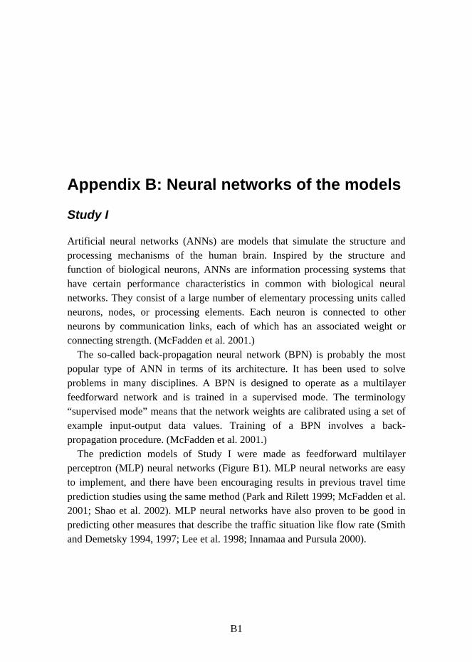
Appendix B: Neural networks of the models

B1

Appendix B: Neural networks of the models

Study I

Artificial neural networks (ANNs) are models that simulate the structure and processing mechanisms of the human brain. Inspired by the structure and function of biological neurons, ANNs are information processing systems that have certain performance characteristics in common with biological neural networks. They consist of a large number of elementary processing units called neurons, nodes, or processing elements. Each neuron is connected to other neurons by communication links, each of which has an associated weight or connecting strength. (McFadden et al. 2001.)

The so-called back-propagation neural network (BPN) is probably the most popular type of ANN in terms of its architecture. It has been used to solve problems in many disciplines. A BPN is designed to operate as a multilayer feedforward network and is trained in a supervised mode. The terminology “supervised mode” means that the network weights are calibrated using a set of example input-output data values. Training of a BPN involves a back-propagation procedure. (McFadden et al. 2001.)

The prediction models of Study I were made as feedforward multilayer perceptron (MLP) neural networks (Figure B1). MLP neural networks are easy to implement, and there have been encouraging results in previous travel time prediction studies using the same method (Park and Rilett 1999; McFadden et al. 2001; Shao et al. 2002). MLP neural networks have also proven to be good in predicting other measures that describe the traffic situation like flow rate (Smith and Demetsky 1994, 1997; Lee et al. 1998; Innamaa and Pursula 2000).

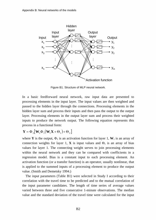
Appendix B: Neural networks of the models

B2

x1

x2

x3

xn

…

……

…

y1

y2

y3

ym

Input OutputInputlayer

Hiddenlayer Output

layer

Activation function

Figure B1. Structure of MLP neural network.

In a basic feedforward neural network, raw input data are presented to processing elements in the input layer. The input values are then weighted and passed to the hidden layer through the connections. Processing elements in the hidden layer sum and process their inputs and then pass the output to the output layer. Processing elements in the output layer sum and process their weighted inputs to produce the network output. The following equation represents this process in a functional form:

( )[ ]211122 Θ+Θ+ΦΦ= XWWY

where Y is the output, Ф1 is an activation function for layer 1, W1 is an array of connection weights for layer 1, X is input values and Θ1 is an array of bias values for layer 1. The connecting weight serves to join processing elements within the neural network and they can be compared with coefficients in a regression model. Bias is a constant input to each processing element. An activation function (or a transfer function) is an operator, usually nonlinear, that is applied to the summed inputs of a processing element to produce the output value. (Smith and Demetsky 1994.)

The input parameters (Table B1) were selected in Study I according to their correlation with the travel time to be predicted and to the mutual correlation of the input parameter candidates. The length of time series of average values varied between three and five consecutive 1-minute observations. The median value and the standard deviation of the travel time were calculated for the input

Appendix B: Neural networks of the models

B3

of either the 10 or 20 latest measured observations or observations of the latest 5 minutes. The input parameters were normalised to have a zero mean and standard deviation of one.

As there was no justification to use a very complex model, a simple structure with one hidden layer was chosen. The number of hidden neurons was chosen with Widrow’s rule of thumb, i.e. the number of training samples was at least ten times the number of parameters to be estimated. However, the number of hidden neurons was limited to no more than 20 to keep the training process fast (Table B2). The activation function of the hidden layer was chosen to be a hyperbolic tangent and that of the output layer a linear function. Innamaa and Pursula (2000) found that this combination provides good results.

Neural networks were trained with the Fletcher–Reeves update (Demuth and Beale 2001), which is one of the conjugate gradient algorithms. In those algorithms, the search is performed along conjugate directions. This produces generally faster convergence than the steepest descent direction, which is a common method in basic back-propagation algorithms. In this study, several stopping conditions were given to prevent the neural network from learning the training data too well. These criteria were the maximum number of training epochs, the minimum values of the gradient and of the mean squared error, and the point at which the mean squared error of the calibration data stopped decreasing.

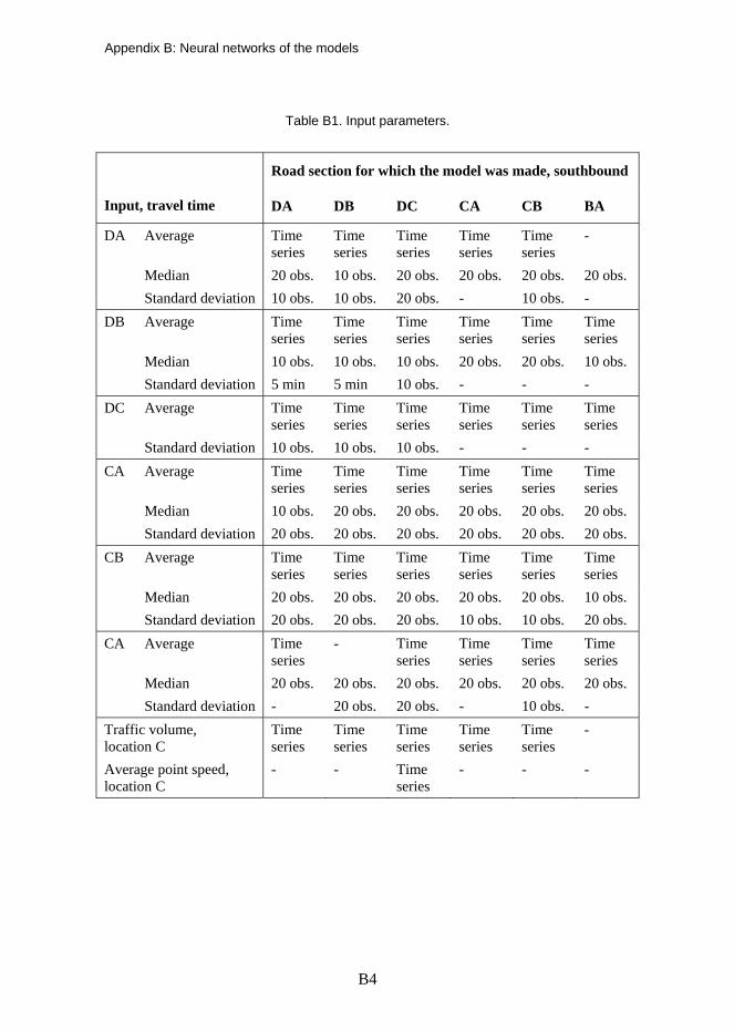
Appendix B: Neural networks of the models

B4

Table B1. Input parameters.

Road section for which the model was made, southbound

Input, travel time DA DB DC CA CB BA

DA Average Time series

Time series

Time series

Time series

Time series

-

Median 20 obs. 10 obs. 20 obs. 20 obs. 20 obs. 20 obs. Standard deviation 10 obs. 10 obs. 20 obs. - 10 obs. - DB Average Time

series Time series

Time series

Time series

Time series

Time series

Median 10 obs. 10 obs. 10 obs. 20 obs. 20 obs. 10 obs. Standard deviation 5 min 5 min 10 obs. - - - DC Average Time

series Time series

Time series

Time series

Time series

Time series

Standard deviation 10 obs. 10 obs. 10 obs. - - - CA Average Time

series Time series

Time series

Time series

Time series

Time series

Median 10 obs. 20 obs. 20 obs. 20 obs. 20 obs. 20 obs. Standard deviation 20 obs. 20 obs. 20 obs. 20 obs. 20 obs. 20 obs. CB Average Time

series Time series

Time series

Time series

Time series

Time series

Median 20 obs. 20 obs. 20 obs. 20 obs. 20 obs. 10 obs. Standard deviation 20 obs. 20 obs. 20 obs. 10 obs. 10 obs. 20 obs. CA Average Time

series - Time

series Time series

Time series

Time series

Median 20 obs. 20 obs. 20 obs. 20 obs. 20 obs. 20 obs. Standard deviation - 20 obs. 20 obs. - 10 obs. - Traffic volume, location C

Time series

Time series

Time series

Time series

Time series

-

Average point speed, location C

- - Time series

- - -

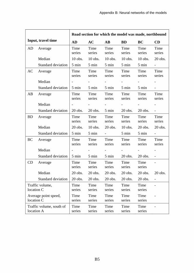
Appendix B: Neural networks of the models

B5

Road section for which the model was made, northbound Input, travel time AD AC AB BD BC CD AD Average Time

series Time series

Time series

Time series

Time series

Time series

Median 10 obs. 10 obs. 10 obs. 10 obs. 10 obs. 20 obs. Standard deviation 5 min 5 min 5 min 5 min 5 min - AC Average Time

series Time series

Time series

Time series

Time series

Time series

Median - - - - - - Standard deviation 5 min 5 min 5 min 5 min 5 min - AB Average Time

series Time series

Time series

Time series

Time series

Time series

Median - - - - - - Standard deviation 20 obs. 20 obs. 5 min 20 obs. 20 obs. - BD Average Time

series Time series

Time series

Time series

Time series

Time series

Median 20 obs. 10 obs. 20 obs. 10 obs. 20 obs. 20 obs. Standard deviation 5 min 5 min - 5 min 5 min - BC Average Time

series Time series

Time series

Time series

Time series

Time series

Median - - - - - - Standard deviation 5 min 5 min 5 min 20 obs. 20 obs. - CD Average Time

series Time series

Time series

Time series

Time series

-

Median 20 obs. 20 obs. 20 obs. 20 obs. 20 obs. 20 obs. Standard deviation 20 obs. 20 obs. 20 obs. 20 obs. 20 obs. - Traffic volume, location C

Time series

Time series

Time series

Time series

Time series

-

Average point speed, location C

Time series

Time series

Time series

Time series

Time series

-

Traffic volume, south of location A

Time series

Time series

Time series

Time series

Time series

-

Appendix B: Neural networks of the models

B6

Table B2. Number of neurons in the input layer and hidden layer of feedforward MLP neural networks. There was one neuron in the output layer, the number of hidden layers was one and the maximum number of neurons in the hidden layer was set to be 20.

Road section for which the model was made, southbound Length of time series Layer DA DB DC CA CB BA

5 min Input 45 41 51 42 44 32 Hidden 14 12 18 19 16 19 4 min Input 38 35 43 35 37 27 Hidden 17 15 20 20 19 20 3 min Input 31 29 35 28 30 22 Hidden 20 18 20 20 20 20

Road section for which the model was made, northbound Length of time series Layer AD AC AB BD BC CD

5 min Input 54 54 53 54 54 28 Hidden 20 20 20 20 20 20 4 min Input 45 45 44 45 45 23 Hidden 20 20 20 20 20 20 3 min Input 36 36 35 36 36 18 Hidden 20 20 20 20 20 20

Appendix B: Neural networks of the models

B7

Study III

The prediction models were constructed as MLP feedforward neural networks (Studies III and IV). The main principles behind the structure of the neural networks were based on the offline models (Study I).

First, the input of the model AD consisted of a time series of the three latest 5-minute observations of median travel time for road sections AD, AC, AB, BD, and BC as well as a time series of the three latest 5-minute observations of traffic volume at the inductive loop detector south of location A and of average point speeds at location C. In the further development stage of model AD, a time series of the travel time on sub-link CD, the mean speed at location C and the traffic volume at the loop detector south of location A, on the other side of the nearby city were also added to the input.

The input of the model DA consisted of a time series of the three latest 5-minute observations of median travel time for road sections DA, DB, and DC and a time series of the three latest 5-minute observations of traffic volume at the inductive loop detector north of location D and at location C.

The number of hidden layers was one and, first, the number of neurons in the hidden layer was 20. The number of input neurons was 21 for the model AD and 15 for the model DA. In the further development stage of model AD, the number of input neurons was 30. The number of hidden neurons was increased from 20 to 30, 40 and 50.

Forecasts were made despite of the partial input. However, the travel time was not predicted if too many or critical detectors were down. In practice, no forecast was made

• if the camera detector was down at the starting point of the road section for which the travel time was predicted

• if more than one camera detector was down

• in the northbound direction AD, if one of camera detectors was down and at the same time the loop detector south of location A was down

• in the southbound direction DA, if one of camera detectors was down and at the same time both the loop detectors were down.

Consequently, there was a separately trained neural network for prediction making for these combinations of working and non-working detectors (Table B3).

Appendix B: Neural networks of the models

B8

Table B3. Combinations of working and non-working detectors for which prediction models were made.

Southbound direction AD

Camera detectors Loop detectors A B C D South of A C

working working working working working working working working working working working down working working working working down working working working working working down down working down working working working working working down working working working down working working down working working working working working down working working down working working working down working working working working working down working down

Northbound direction DA

Camera detectors Loop detectors D C B A North of D C

working working working working working working working working working working down working working working working working working down working working working working down down working down working working working working working down working working down working working down working working working down working working down working working working working working down working down working working working down working working down working working working down working working working working working down down working working working working down working down

Appendix B: Neural networks of the models

B9

Study V

The prediction models of Study V included self-organising maps (SOM, Kohonen 2001). A SOM consists of neurons (processing units or map units) organised on a regular low-dimensional grid (feature map, Figure B2). Distances between the map units can be measured by the distance of their weight vectors in grid coordinates. In this study, the Euclidian distance was used. The Euclidean distance between points P = (p1, p2, …, pn) and Q = (q1, q2, …, qn), in Euclidean n-space, is defined as:

( ) ( ) ( ) ( )∑=

−=−++−+−n

iiinn qpqpqpqp

1

22222

211

Figure B2. Structure of SOM.

SOMs were made based on the principles of supervised learning. Supervised learning proceeds in the same way as the unsupervised basic method. However, the class information is added to the patterns in the training phase. Consequently, the separation of classes is better than with unsupervised learning. SOMs were trained with a batch-training algorithm (Vesanto et al. 2000).

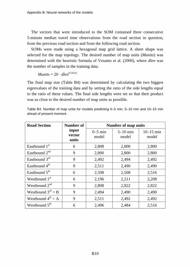
Appendix B: Neural networks of the models

B10

The vectors that were introduced to the SOM contained three consecutive 5-minute median travel time observations from the road section in question, from the previous road section and from the following road section.

SOMs were made using a hexagonal map grid lattice. A sheet shape was selected for the map topology. The desired number of map units (Munits) was determined with the heuristic formula of Vesanto et al. (2000), where dlen was the number of samples in the training data.

Munits = 20 · dlen0.54321

The final map size (Table B4) was determined by calculating the two biggest eigenvalues of the training data and by setting the ratio of the side lengths equal to the ratio of these values. The final side lengths were set so that their product was as close to the desired number of map units as possible.

Table B4. Number of map units for models predicting 0–5 min, 5–10 min and 10–15 min ahead of present moment.

Number of map units Road Section Number of input vector units

0–5 min model

5–10 min model

10–15 min model

Eastbound 1st 6 2,808 2,800 2,800 Eastbound 2nd 9 2,800 2,800 2,800 Eastbound 3rd 9 2,492 2,494 2,492 Eastbound 4th 9 2,511 2,490 2,490 Eastbound 5th 6 2,508 2,508 2,516 Westbound 1st 6 2,196 2,211 2,208 Westbound 2nd 9 2,808 2,822 2,822 Westbound 3rd = B 9 2,494 2,490 2,490 Westbound 4th = A 9 2,511 2,492 2,492 Westbound 5th 6 2,496 2,484 2,516

Series title, number and report code of publication

VTT Publications 708 VTT-PUBS-708

Author(s)

Satu Innamaa Title

Short-term prediction of traffic flow status for online driver information

Abstract The principal aim of this study was to develop a method for making a short-term prediction model of traffic flow status (i.e. travel time and a five-step travel-speed-based classification) and test its performance in the real world environment. Specifically, the objective was to find a method that can predict the traffic flow status on a satisfactory level, can be implemented without long delays and is practical for real-time use also in the long term. A sequence of studies shows the development process from offline models with perfect data to online models with field data. Models were based on MLP neural networks and self-organising maps. The purpose of the online model was to produce real-time information of the traffic flow status that can be given to drivers. The models were tested in practice. In conclusion, the results of online use of the prediction models in practice were promising and even a simple prediction model was shown to improve the accuracy of travel time information especially in congested conditions. The results also indicated that the self-adapting principle improved the performance of the model and made it possible to implement the model quite quickly. The model was practical for real-time use also in the long term in terms of the number of carry bits that it requires to restore the history of samples of traffic situations. As self-adapting this model performed better than as a static version i.e. without the self-adapting feature, as the proportion of correctly predicted traffic flow status increased considerably for the self-adapting model during the online trial. ISBN 978-951-38-7340-0 (soft back ed.) 978-951-38-7341-7 (URL: http://www.vtt.fi/publications/index.jsp )

Series title and ISSN Project number VTT Publications 1235-0621 (soft back ed.) 1455-0849 (URL: http://www.vtt.fi/publications/index.jsp)

34472

Date Language Pages May 2009 English, Finnish abstr. 79 p. + app. 90 p.

Name of project Commissioned by

Keywords Sold by prediction, traffic flow status, travel time VTT Technical Research Centre of Finland

P.O. Box 1000, FI-02044 VTT, Finland Phone internat. +358 20 722 4520 Fax +358 20 722 4374

Julkaisun sarja, numero ja raporttikoodi

VTT Publications 708 VTT-PUBS-708

Tekijä(t) Satu Innamaa

Nimeke

Liikennetilanteen lyhyen aikavälin ennustaminen ajantasaisen kuljettajatiedotuksen tarpeisiin Tiivistelmä

Tutkimuksen päätavoitteena oli kehittää menetelmä liikennetilanteen lyhyen aikavälin ennustamiseen ja testata sen toimivuus todellisissa liikenneolosuhteissa. Tässä liikennetilanteella tarkoitetaan matka-aikaa ja viisiportaista matka-aikaan perustuvaa luokittelua. Erityisesti tavoitteena oli löytää liikennetilannetta tyydyttävästi ennustava menetelmä, joka voidaan ottaa käyttöön ilman pitkiä viipeitä ja joka on käytännöllinen ajantasaisessa käytössä myös pitkällä aikavälillä. Tutkimussarja näyttää kehitysprosessin täydelliseen aineistoon perustuvista tutkimusmalleista maastosta mitattua aineistoa käyttäviin ajantasaisiin malleihin. Mallit perustuivat MLP-neuroverkkoihin ja itseorgani-soituviin karttoihin. Ajantasaisen mallin tarkoituksena on tuottaa reaaliaikaista tietoa liikennevirran tilasta kuljettajille välitettäväksi. Malleja testattiin käytännön olosuhteissa. Ajantasaisesta käytöstä saatujen tulosten perusteella ennustemallit vaikuttivat lupaavilta, ja jopa yksinkertaisen ennustemallin voitiin osoittaa parantavan matka-aikatiedon tarkkuutta erityisesti ruuhkassa. Tulokset osoittivat myös, että itseoppimisen periaate paransi mallin suorituskykyä ja mahdollisti mallin suhteellisen nopean käyttöönoton. Malli oli tarkoituksenmukainen ajantasaisessa käytössä myös pitkällä aikavälillä, sillä se vaati erittäin vähän muistitilaa liikennetilannehistorian tallentamiseen. Itseoppivana malli toimi paremmin kuin staattisena versiona eli ilman itseoppimisperiaatetta, sillä oikein ennus-tettujen liikennetilanteiden osuus kasvoi itseoppivalla mallilla huomattavasti käyttökokei-lun aikana. ISBN 978-951-38-7340-0 (nid.) 978-951-38-7341-7 (URL: http://www.vtt.fi/publications/index.jsp)

Avainnimeke ja ISSN Projektinumero VTT Publications 1235-0621 (nid.) 1455-0849 (URL: http://www.vtt.fi/publications/index.jsp)

34472

Julkaisuaika Kieli Sivuja Toukokuu 2009 Englanti, suom. tiiv. 79 s. + liitt. 90 s.

Projektin nimi Toimeksiantaja(t)

Avainsanat Julkaisija

prediction, traffic flow status, travel time VTT PL 1000, 02044 VTT Puh. 020 722 4520 Faksi 020 722 4374

Dissertation VTT PUBLICATIONS 708VTT CREATES BUSINESS FROM TECHNOLOGY�Technology�and�market�foresight�•�Strategic�research�•�Product�and�service�development�•�IPR�and�licensing�•�Assessments,�testing,�inspection,�certification�•�Technology�and�innovation�management�•�Technology�partnership

•�•�•��VTT�PUB

LICA

TION

S�708���SHO

RT-TER

M�PR

EDIC

TION

�OF�TR

AFFIC

�FLOW

�STATU

S�FOR

�ON

LINE�D

RIVER

�INFO

RM

ATIO

N

ISBN 978-951-38-7340-0 (soft back ed.) ISBN 978-951-38-7341-7 (URL: http://www.vtt.fi/publications/index.jsp)ISSN 1235-0621 (soft back ed.) ISSN 1455-0849 (URL: http://www.vtt.fi/publications/index.jsp)

Satu Innamaa

Short-term prediction of traffic flow status for online driver information

The studies described in this dissertation developed a method for making a short-term prediction model of traffic flow status and tested its performance in the real world environment. Study sites were an interurban two-lane two-way highway section and an urban multilane corridor with varying standard. Online use of short-term prediction models in practice was promising and even a simple prediction model was shown to improve the accuracy of travel time information especially in congested conditions. The results also indicated that the self-adapting principle improved the performance of the model and made it possible to implement the model quite quickly. As self-adapting this model performed better than without the self-adapting feature. The model was practical for real-time use also in the long term. The dissertation sums up five studies on modelling of traffic flow status for short-term prediction. These studies show the development process from offline models that use perfect data to online models that deal directly with field-measured data. The purpose of the online model was to produce real-time information that can be given to drivers.