Shin-ichi Sasa arXiv:1703.08946v2 [cond-mat.stat … · Yuki Minami · Shin-ichi Sasa September 13, 2017 Abstract We study a noisy Kuramoto-Sivashinsky (KS) equation which describes

arX

iv:1

703.

0894

6v2

[co

nd-m

at.s

tat-

mec

h] 1

2 Se

p 20

17

Noname manuscript No.

(will be inserted by the editor)

The most effective model for describing the universal behavior of unstable

surface growth

Yuki Minami · Shin-ichi Sasa

September 13, 2017

Abstract We study a noisy Kuramoto-Sivashinsky (KS) equation which describes unstable surfacegrowth and chemical turbulence. It has been conjectured that the universal long-wavelength behaviorof the equation, which is characterized by scale-dependent parameters, is described by a Kardar-Parisi-Zhang (KPZ) equation. We consider this conjecture by analyzing a renormalization-group equation fora class of generalized KPZ equations. We then uniquely determine the parameter values of the KPZequation that most effectively describes the universal long-wavelength behavior of the noisy KS equation.

Keywords renormalization group methods · nonlinear dynamics · Stochastic process · Surface growth

1 Introduction

Eddy viscosity in turbulence, which can explain how a vortex pattern emerges in a non-uniform turbulentflow, depends on the observed length scales [1]. As exemplified by the Richardson law [2], there arecases in which a parameter of a macroscopic description is not given as a definite value, but is ratherexpressed as a function of the length scale. Another example of scale-dependent parameters has beenobserved in one- or two- dimensional fluid dynamics, where the viscosity is not uniquely defined in thehydrodynamic description [3]. Here, it seems reasonable to expect that such scale-dependent parametersin a macroscopic description can be reproduced by an effective stochastic system [4,5,6,7,8,9,10,11]. Inthis paper, we attempt to determine the effective stochastic system theoretically when scale-dependentparameters are observed.

As the simplest example for scale-dependent parameters, we consider the one-dimensional Kardar-Parisi-Zhang (KPZ) equation [12]. It is known that the effective surface tension ν(Λ) at a scale 2π/Λ forthe equation is ν(Λ) = CνΛ

−1/2 in the limit Λ → 0, which is similar to the Richardson law for turbulence.Recently, the KPZ equation was rigorously derived from a stochastic many-particle model [13,14], andthe so-called KPZ class has been extensively discussed both theoretically and experimentally [15,16,17,18,19,20]. However, in general, even if we find systems that may exhibit scale-dependent parameterssimilar to those for the KPZ class, a method to determine the parameter values of the correspondingKPZ equation has not yet been reported.

Specifically, let us consider a noisy Kuramoto-Sivashinsky (KS) equation, which exhibits spatiallyextended chaos in the noiseless limit [21,22,23]. The model describes turbulent chemical waves andunstable interface motions, which are caused by negative surface tension. It has been conjectured thata KPZ equation may be an effective model for describing the long-wavelength behavior of the noisyKS equation; this conjecture is referred to as the Yakhot conjecture [24,25]. Indeed, direct numerical

Y. MinamiNational Institute of Advanced Industrial Science and Technology (AIST), Ibaraki 305-8560, JapanE-mail: [email protected]

S. SasaDepartment of Physics, Kyoto University, Kyoto 606-8502, JapanE-mail: [email protected]

http://arxiv.org/abs/1703.08946v2

2 Yuki Minami, Shin-ichi Sasa

simulations showed that statistical properties of the long wave length modes are similar to those of theKPZ equations [26,27,28,29,30].

Here, one may recall the renormalization group (RG), which is a standard method for studyingscale-dependent parameters. For a given noisy KS equation, the RG equation was calculated using aperturbation theory [30,31]. The infrared fixed point of the RG equation determines the scale-dependentbehavior ν(Λ) = CνΛ

−1/2 in the limit Λ → 0, which has the same power-law form as that for the KPZequations. Nevertheless, as shown below, the analysis at the infrared fixed point of the RG equationcannot determine the parameter values of the corresponding KPZ equation.

In this paper, we present a framework for studying the effective description. We study an RG equationfor generalized KPZ equations that include noisy KS equations and KPZ equations. We then considersolution trajectories of the RG equation, in which each point flows to the infrared fixed point of the noisyKS equation we study. The solution trajectories also approach a subspace in the ultraviolet limit, whichenables us to define a collection of bare parameters of the generalized KPZ equations. By using the lowestperturbation theory for the RG equation, we uniquely determine the most effective model among suchKPZ equations that describes the infrared universal behavior of a noisy KS equation in the most efficientmanner.

This paper is organized as follows. In Sect. 2, we introduce a class of models we study, define scale-dependent parameters for the models, and review RG equations for the parameters. We also discussultraviolet and infrared behaviors of solution trajectories for the RG equation, and classify universaland non-universal properties of those. After that, we give a definition of “the most effective model”.In Sect. 3, we simplify a representation of the trajectories so as to determine the most effective model.The solution trajectories for the RG equation are expressed as curves in a five-dimensional parameterspace. Then, the trajectory for the noisy KS equation is attracted to a two-dimensional subspace, due toemergence of a time-reversal symmetry. We define the most effective model for the noisy KS equation inthis subspace. In Sect. 4, we determine parameter values of the most effective model from its definition. InSect. 5, we provide concluding remarks. We discuss renormalizability of the KPZ equation and its relevantparameters. We also remark an another application of our formalism to turbulence. In Appendix A, wederive Ward-Takahashi identities for scale-dependent parameters from symmetries of our model.

2 Setup

We study models for the stochastic growth of a surface. We assume that the time evolution of the heighth(x, t) of the surface is described by a generalized KPZ equation:

∂th = ν∂2xh−K∂4

xh+λ

2(∂xh)

2 + η, (1)

〈η(x, t)η(x′

, t′

)〉 = 2(D −Dd∂2x)δ(t− t

′

)δ(x− x′

), (2)

where ν is the surface tension, K is the surface diffusion constant, λ is the strength of the non-linearity,and η(x, t) is the white noise. Here, D and Dd are the strength of the noise. When K = Dd = 0, (2) isthe KPZ equation, while when D = Dd = 0, (2) with ν < 0 is the deterministic KS equation. We refer to(2) with ν < 0 and K,D,Dd > 0, as the noisy KS equation.

The five parameters in (2) are collectively denoted by X ≡ (ν,K,D,Dd, λ). More precisely, theseparameters are defined for a field h(x) whose Fourier transform h(k) is assumed to be zero for |k| > Λ.Λ is called a cut-off wavenumber. We explicitly express the cutoff dependence of the parameters asX (Λ). Here, for a given model with X (Λ0), we define a model with X (Λ) for Λ < Λ0 by eliminating thecontribution Λ ≤ |k| ≤ Λ0 in the dynamics, which may be formally expressed as X (Λ;X (Λ0)). Note thatwe do not employ a rescaling transformation after the coarse-graining. This functional relation triviallysatisfies

X (Λ′;X (Λ0)) = X (Λ′;X (Λ;X (Λ0))). (3)

From this, we obtain the RG equation

−ΛdXdΛ

= ΨX (X ), (4)

which determines X (Λ;X (Λ0)) under an initial condition X (Λ0) = X0. In the next subsection, we reviewthe RG equation for the generalized KPZ equations.

The most effective model for the universal behavior of unstable surface growth 3

2.1 definition of scale-dependent parameters

We first define the scale-dependent parameters ν(Λ), D(Λ), K(Λ), Dd(Λ) and λ(Λ), and then introducea perturbation theory leading to the equation for determining them.

We start with the generating functional Z[J, J] by which all statistical quantities of the KPZ equationsare determined. Following the Martin-Siggia-Rose-Janssen-deDominicis (MSRJD) formalism [32,33,34,35], Z[J, J ] is expressed as

Z[J, J ] =

∫

D[h, ih] exp

[

−S[h, ih;Λ0]

+

∫ ∞

−∞

dω

∫ Λ0

−Λ0

dk

(

J(k, ω)h(−k,−ω) + J(k, ω)ih(−k,−ω)

)]

, (5)

where ih is the auxiliary field, J and J are source fields, and S[h, ih;Λ0] is the MSRJD action for thegeneralized KPZ equation. Hereafter, we use the notation A(k,ω) for the Fourier transform of A(x, t) forany field A. The action S[h, ih;Λ0] is explicitly written as

S[h, ih;Λ0] =1

2

∫ ∞

−∞

dω

2π

∫ Λ0

−Λ0

dk

2π

(

h(−k,−ω) ih(−k,−ω))

G−10 (k, ω)

(

h(k, ω)

ih(k, ω)

)

+λ0

2

∫ ∞

−∞

dω1dω2

(2π)2

∫ Λ0

−Λ0

dk1dk2(2π)2

k1k2ih(−k1 − k2,−ω1 − ω2)h(k1, ω1)h(k2, ω2), (6)

where G−10 is the inverse matrix of the bare propagator

G−10 (k, ω) =

(

0 iω + ν0k2 +K0k

4

−iω + ν0k2 +K0k

4 −2(D0 +Dd0k2)

)

. (7)

Here, we consider a coarse-grained description at a cutoff Λ < Λ0. Let us define

A<(k,ω) ≡ θ(Λ− k)A(k,ω), (8)

A>(k,ω) ≡ θ(k − Λ)A(k,ω), (9)

for any quantity A(k,ω), where θ(x) is the Heaviside step function. The statistical quantities of h< aredescribed by the generating functional Z[J<, J<] with replacement of (J, J) by (J<, J<). We thus definethe effective MSRJD action S[h<, ih<;Λ] by the relation

Z[J<, J<] =

∫

D[h<, ih<] exp

[

−S[h<, ih<;Λ]

+

∫ ∞

−∞

dω

∫ Λ

−Λ

dk

(

J<(k, ω)h<(−k,−ω) + J<(k, ω)ih<(−k,−ω)

)]

. (10)

We can then confirm that S[h<, ih<;Λ] is determined as

exp

[

−S[h<, ih<;Λ]

]

=

∫

D[h>, ih>] exp

[

−S[h< + h>, ih< + ih>;Λ0]

]

. (11)

Then, the propagator and the three point vertex function for the effective MSRJD action at Λ are definedas

(G−1)hh(k1, ω1;Λ)δ(ω1 + ω2)δ(k1 + k2) ≡δ2S[h<, ih<;Λ]

δ(ih(k1, ω1))δ(h<(k2, ω2))

∣

∣

∣

∣

h<,ih<=0

, (12)

(G−1)hh(k1, ω1;Λ)δ(ω1 + ω2)δ(k1 + k2) ≡δ2S[h<, ih<;Λ]

δ(ih<(k1, ω1))δ(ih<(k2, ω2))

∣

∣

∣

∣

h<,ih<=0

, (13)

Γhhh(k1, ω1; k2, ω2;Λ)δ(ω1 + ω2 + ω3)δ(k1 + k2 + k3)

≡ δ3S[h<, ih<;Λ]

δ(ih<(k1, ω1))δ(h<(k2, ω2))δ(h<(k3, ω3))

∣

∣

∣

∣

h<,ih<=0

. (14)


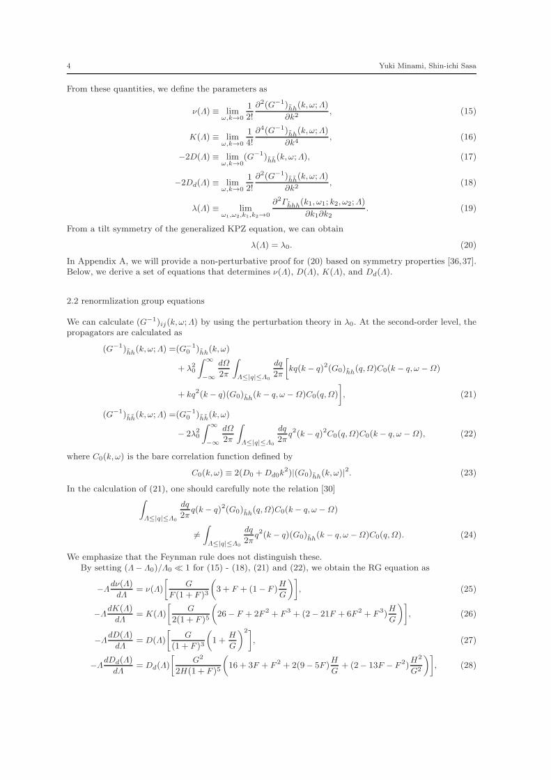
From these quantities, we define the parameters as

ν(Λ) ≡ limω,k→0

1

2!

∂2(G−1)hh(k,ω;Λ)

∂k2, (15)

K(Λ) ≡ limω,k→0

1

4!

∂4(G−1)hh(k,ω;Λ)

∂k4, (16)

−2D(Λ) ≡ limω,k→0

(G−1)hh(k, ω;Λ), (17)

−2Dd(Λ) ≡ limω,k→0

1

2!

∂2(G−1)hh(k,ω;Λ)

∂k2, (18)

λ(Λ) ≡ limω1,ω2,k1,k2→0

∂2Γhhh(k1, ω1; k2, ω2;Λ)

∂k1∂k2. (19)

From a tilt symmetry of the generalized KPZ equation, we can obtain

λ(Λ) = λ0. (20)

In Appendix A, we will provide a non-perturbative proof for (20) based on symmetry properties [36,37].Below, we derive a set of equations that determines ν(Λ), D(Λ), K(Λ), and Dd(Λ).

2.2 renormlization group equations

We can calculate (G−1)ij(k,ω;Λ) by using the perturbation theory in λ0. At the second-order level, thepropagators are calculated as

(G−1)hh(k, ω;Λ) =(G−10 )hh(k,ω)

+ λ20

∫ ∞

−∞

dΩ

2π

∫

Λ≤|q|≤Λ0

dq

2π

[

kq(k − q)2(G0)hh(q,Ω)C0(k − q, ω −Ω)

+ kq2(k − q)(G0)hh(k − q, ω −Ω)C0(q,Ω)

]

, (21)

(G−1)hh(k, ω;Λ) =(G−10 )hh(k,ω)

− 2λ20

∫ ∞

−∞

dΩ

2π

∫

Λ≤|q|≤Λ0

dq

2πq2(k − q)2C0(q,Ω)C0(k − q, ω −Ω), (22)

where C0(k, ω) is the bare correlation function defined by

C0(k,ω) ≡ 2(D0 +Dd0k2)|(G0)hh(k, ω)|

2. (23)

In the calculation of (21), one should carefully note the relation [30]∫

Λ≤|q|≤Λ0

dq

2πq(k − q)2(G0)hh(q,Ω)C0(k − q, ω −Ω)

6=∫

Λ≤|q|≤Λ0

dq

2πq2(k − q)(G0)hh(k − q, ω −Ω)C0(q,Ω). (24)

We emphasize that the Feynman rule does not distinguish these.By setting (Λ− Λ0)/Λ0 ≪ 1 for (15) - (18), (21) and (22), we obtain the RG equation as

−Λdν(Λ)

dΛ= ν(Λ)

[

G

F (1 + F )3

(

3 + F + (1− F )H

G

)]

, (25)

−ΛdK(Λ)

dΛ= K(Λ)

[

G

2(1 + F )5

(

26− F + 2F 2 + F 3 + (2− 21F + 6F 2 + F 3)H

G

)]

, (26)

−ΛdD(Λ)

dΛ= D(Λ)

[

G

(1 + F )3

(

1 +H

G

)2]

, (27)

−ΛdDd(Λ)

dΛ= Dd(Λ)

[

G2

2H(1 + F )5

(

16 + 3F + F 2 + 2(9− 5F )H

G+ (2− 13F − F 2)

H2

G2

)]

, (28)


where we have introduced the dimensionless parameters F , G and H as

F =ν(Λ)

K(Λ)Λ2, (29)

G =λ20D(Λ)

4πK3(Λ)Λ7, (30)

H =λ20Dd(Λ)

4πK3(Λ)Λ5. (31)

Here, from (25)-(28), we derive the autonomous equation for (F (Λ),G(Λ),H(Λ)) as

−ΛdF

dΛ= 2F +

G

2(1 + F )5

[

6− 12F + 11F 2 − F 4 + (2 + 19F 2 − 8F 3 − F 4)H

G

]

, (32)

−ΛdG

dΛ= 7G− G2

2(1 + F )5

[

76− 7F + 4F 2 + 3F 3 + (2− 71F + 14F 2 + 3F 3)H

G

− 2(1 + F )2H2

G2

]

, (33)

−ΛdH

dΛ= 5H +

G2

2(1 + F )5

[

16 + 3F + F 2 − (60 + 7F + 6F 2 + 3F 3)H

G

− (4− 50F + 19F 2 + 3F 3)H2

G2

]

. (34)

2.3 Infrared and ultraviolet behaviors of solution trajectories of the RG equation

The stable fixed point of the equations (32) - (34) is found to be (F ∗, G,∗ , H∗) = (10.7593, 680.652, 63.2614).By substituting the fixed point values to (25)-(28) and solving them, we obtain the scaling laws

ν(Λ) = CνΛ−0.5, (35)

D(Λ) = CDΛ−0.5, (36)

K(Λ) = CKΛ−2.5, (37)

Dd(Λ) = CDdΛ−2.5, (38)

where Cν , CD, CK , and CDdare constants that depend on the initial condition X0.

We next consider the dimensionless quantities given by

1

F=

K(Λ)Λ2

ν(Λ), (39)

H

G=

Dd(Λ)Λ2

D(Λ). (40)

Substituting the scaling relations (35) - (38) to these equalities, we have

1

F ∗ =CK

Cν,

H∗

G∗ =CDd

CD. (41)

Since (F,G,H) takes the value (10.7593, 680.652, 63.2614) in the limit Λ → 0, we obtain

CK

Cν=

CDd

CD= 0.0929, (42)

which is independent of X0 . The singular behavior ν(Λ) = CνΛ−1/2 implies that the effective surface

tension depends on the observed scale Λ. This is contrasted with cases in which each X (Λ) converges


to a finite value in the limit Λ → 0. Then, X (Λ = 0) is interpreted as renormalized parameters mea-sured in experiments. Since the exponents characterizing the divergent behaviors are common to all themodels given by (2), we refer to the power-law region as the universal range. The smallest characteristicwavenumber scale is also denoted by ΛIR, the value of which depends on X0. Then, the universal rangeis defined as Λ ≪ ΛIR. As another common aspect of the RG equation (4), we observe that X (Λ) shows aplateau region in the ultraviolet limit when Λ0 is sufficiently large. This enables us to define a collectionof bare parameters, which is denoted by XB .

0

10

20

30

40

50

10-1

100

101

102

103

104

Λ-1

ν(Λ)

D(Λ)10

0

102

104

10-1

101

103

Λ-1

K(Λ)Dd(Λ)

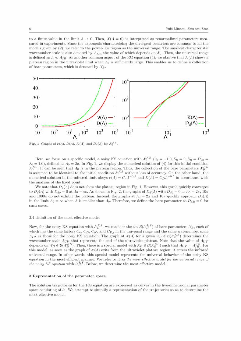
Fig. 1 Graphs of ν(Λ), D(Λ), K(Λ), and Dd(Λ) for XKS0 .

Here, we focus on a specific model, a noisy KS equation with XKS0 , (ν0 = −1.0, D0 = 0,K0 = Dd0 =

λ0 = 1.0), defined at Λ0 = 2π. In Fig. 1, we display the numerical solution of (4) for this initial conditionXKS0 . It can be seen that Λ0 is in the plateau region. Thus, the collection of the bare parameters XKS

B

is assumed to be identical to the initial condition XKS0 without loss of accuracy. On the other hand, the

numerical solution in the infrared limit obeys ν(Λ) = CνΛ−0.5 and D(Λ) = CDΛ−0.5 in accordance with

the analysis of the fixed point.We note that Dd(Λ) does not show the plateau region in Fig. 1. However, this graph quickly converges

to Dd(Λ) with Dd0 = 0 at Λ0 = ∞. As shown in Fig. 2, the graphs of Dd(Λ) with Dd0 = 0 at Λ0 = 2π, 10πand 1000π do not exhibit the plateau. Instead, the graphs at Λ0 = 2π and 10π quickly approach Dd(Λ)in the limit Λ0 = ∞ when Λ is smaller than Λ0. Therefore, we define the bare parameter as DdB = 0 forsuch cases.

2.4 definition of the most effective model

Now, for the noisy KS equation with XKSB , we consider the set B(XKS

B ) of bare parameters XB , each ofwhich has the same factors Cν , CD, CK , and CDd

in the universal range and the same wavenumber scaleΛIR as those for the noisy KS equation. The graph of X (Λ) for a given XB ∈ B(XKS

B ) determines thewavenumber scale ΛUV that represents the end of the ultraviolet plateau. Note that the value of ΛUV

depends on XB ∈ B(XKSB ). Then, there is a special model with XB ∈ B(XKS

B ) such that ΛUV = ΛKSIR . For

this model, as soon as the graph of X (Λ) exits from the ultraviolet plateau region, it enters the infrareduniversal range. In other words, this special model represents the universal behavior of the noisy KSequation in the most efficient manner. We refer to it as the most effective model for the universal range of

the noisy KS equation with XKSB . Below, we determine the most effective model.

3 Representation of the parameter space

The solution trajectories for the RG equation are expressed as curves in the five-dimensional parameterspace consisting of X . We attempt to simplify a representation of the trajectories so as to determine themost effective model.


10-24

10-20

10-16

10-12

10-8

10-4

10-2

10-1

Dd(Λ

)

Λ-1

Λ0=2πΛ0=10π

Λ0=1000π

Fig. 2 Graphs of Dd(Λ) for XKS0 at Λ0 = 2π, 10π and 1000π.

-4

-2

0

2

4

6

100

101

102

103

104

Λ-1

D/νDd/K

Fig. 3 Graphs of D(Λ)/ν(Λ) and Dd(Λ)/K(Λ) for XKSB . D(Λ)/ν(Λ) and Dd(Λ)/K(Λ) converge to the same value,

2.24.

First, recalling λ(Λ) = λ0, we may restrict the parameter space into the subspace λ = λ0 = 1.Next, as shown in Fig. 3, we find that D(Λ)/ν(Λ) and Dd(Λ)/K(Λ) converge to the same value, 2.24,

in the universal range for the noisy KS equation. We can explain this phenomenon as follows. First,for the generalized KPZ equations with XB satisfying DB/νB = DdB/KB ≡ χ > 0, we can show thefluctuation-dissipation relation with the effective temperature χ fixed by using a time-reversal symmetry.The time-reversal transformation is given as

h′

(k, ω) = −h(k,−ω), (43)

h′

(k, ω) = h(k,−ω)− ν0k2

D0h(k,−ω). (44)

The variation of the action (6) under this transformation is calculated as

δS ≡S[h′

, ih′

;Λ0]− S[h, ih;Λ0],

=

(

D0

ν0− Dd0

K0

)

ν0K0

D0

∫

dωdk

(2π)2

(

ν0D0

k2h(−k,−ω)h(k,ω)− 2ih(−k,−ω)h(k,ω)

)

. (45)


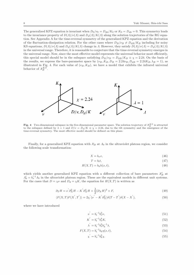
The generalized KPZ equation is invariant when D0/ν0 = Dd0/K0 or K0 = Dd0 = 0. This symmetry leadsto the invariance property of D(Λ)/ν(Λ) and Dd(Λ)/K(Λ) along the solution trajectories of the RG equa-tion. See Appendix A for the time-reversal symmetry of the generalized KPZ equation and the derivationof the fluctuation-dissipation relation. For the other cases where DB/νB 6= DdB/KB including for noisyKS equations, D(Λ)/ν(Λ) and Dd(Λ)/K(Λ) change in Λ. However, they satisfy D(Λ)/ν(Λ) = Dd(Λ)/K(Λ)in the universal range. Therefore, it is reasonable to conjecture that the time-reversal symmetry emerges inthe universal range. Now, since the most effective model represents the universal behavior most efficiently,this special model should be in the subspace satisfying DB/νB = DdB/KB ≡ χ = 2.24. On the basis ofthe results, we express the bare-parameter space by (νB ,KB , DB = 2.24νB, DdB = 2.24KB, λB = 1), asillustrated in Fig. 4. For each value of (νB ,KB), we have a model that exhibits the infrared universalbehavior of XKS

B .

Fig. 4 Two-dimensional subspace in the five-dimensional parameter space. The solution trajectory of XKSB is attracted

to the subspace defined by λ = 1 and D/ν = Dd/K ≡ χ = 2.24, due to the tilt symmetry and the emergence of thetime-reversal symmetry. The most effective model should be defined on this plane.

Finally, for a generalized KPZ equation with XB at Λ0 in the ultraviolet plateau region, we considerthe following scale transformation:

X = bxx, (46)

T = btt, (47)

H(X,T ) = bhh(x, t), (48)

which yields another generalized KPZ equation with a different collection of bare parameters X ′B at

Λ′0 = b−1

x Λ0 in the ultraviolet plateau region. These are the equivalent models in different unit systems.For the cases that D = χν and Dd = χK, the equation for H(X,T ) is written as

∂TH = ν′

∂2XH −K

′

∂4XH +

λ

2(∂XH)2 + F, (49)

〈F (X,T )F (X′

, T′

)〉 = 2χ′

(ν′

−K′

∂2X)δ(T − T

′

)δ(X −X′

), (50)

where we have introduced

ν′

= b−1t b2xν, (51)

K′

= b−1t b4xK, (52)

λ′

= b−1t b2xb

−1h λ, (53)

F (X,T ) = b−1t bhη(x, t), (54)

χ′

= b−1x b2hχ. (55)


By imposing χ′ = χ and λ′ = λ, we obtain bh = b1/2x and bt = b

3/2x . Then, we have the relation

ν′

B = b1/2x νB , (56)

K′

B = b5/2x KB , (57)

We find that J ≡ KB/ν5B is invariant under the transformation. Thus, we parameterize (νB ,KB) as

(b1/2x , b

5/2x J). The next problem is to determine the values of bx and J of the most effective model for the

universal range of the noisy KS equation.

4 the most effective model

Since J is invariant under the scale transformation, the determination of J can be separated from thedetermination of bx. Here, we notice the condition ΛUV = ΛIR for the most effective model. Because thiscondition is invariant under the scale transformation, the value of J is uniquely determined. Furthermore,the condition ΛIR = ΛKS

IR fixes the value of bx. Below, we explicitly calculate these values.

-8

-4

0

4

8

-2 0 2 4 6 8

F-F

*

s

J=0.1

J=1.0

J=7.3

J=20-0.010

-0.005

0.000

2 4 6 8

F-F

*

s

J=7.1

J=7.2

J=7.3

J=7.4

Fig. 5 Graphs of F − F ∗ as a function of s ≡ − ln(J1/2bxΛ) for several J .

In order to determine the value of J, we study the dimensionless quantity F (Λ) = ν(Λ)/(K(Λ)Λ2) asa function of

s(Λ) ≡ − ln(J1/2bxΛ), (58)

where F and s are invariant under the scale transformation. It should be noted that, for any J and bx,F approaches

F → e2s, (59)

in the ultraviolet limit s → −∞, while

F → F ∗ = 10.76, (60)

in the infrared limit s → ∞. In Fig. 5, we show graphs of F as functions of s for several values of J. Ingeneral, there are two characteristic scales of s, the departure scale from e2s and the relaxation scale toF ∗, as clearly observed for J = 0.1. When J increases, the peak of F decreases and eventually vanishesat J = 7.3. In this case, the transition scale between the infrared universal region and the ultravioletregion is simply given by the cross point sc of the ultraviolet behavior F = e2s and the infrared behaviorF ∗ = 10.8. That is,

e2sc = F ∗, (61)


10-4

10-3

10-2

10-1

100

101

0 200 400 600Λ-1

KS

fitted curve

10-2

10-1

100

101

100

102

104

Λ-1

KS

Λ0.43

Fig. 6 Graphs of |ν(Λ) − CνΛ−1/2 + AΛB| for XKSB and the fitted curve in the left panel. The right panel shows the

graphs of |ν(Λ)− CνΛ−1/2| and AΛB with A = 3.57 and B = 0.431.

which gives sc = 1.2. Thus, we conclude that the value of J of the most effective model is J = 7.3.Next, we determine the value of bx. From the cross point sc, we define the transition length scale

Λ−1c by sc = − ln(J1/2bxΛc), which gives Λ−1

c =√JF ∗bx = 8.9bx. Here, the value of bx is determined

by identifying Λc with ΛKSIR . Then, we estimate ΛKS

IR from the graph of ν(Λ) for the noisy KS equationunder study. In Fig. 6, we show how ν(Λ) approaches CνΛ

−0.5. We find that |ν(Λ)−CνΛ−0.5| is well fitted

to a power-law function of Λ−1, which does not provide any wavenumber scale. Through more detailedanalysis, we find a fitting function

ν(Λ)− CνΛ−0.5 = −AΛB + C exp

[

−Λ−1

D

]

, (62)

with A = 3.57, B = 0.431, C = 1.1 × 10−2, and D = 195. From the second term of (62), we obtain thecharacteristic scale (ΛKS

IR )−1 = D = 195. Now, from the condition

(ΛKSIR )−1 = Λ−1

c , (63)

we obtain bx = 22. Thus, we have arrived at the most effective model for the universal range of the noisyKS equation with XKS

B , where the collection of the bare parameter values of the most effective model,XMEB , is determined as (νB = 4.7,DB = 10,KB = 1.6× 104, DdB = 3.7× 104, λB = 1).Now, the linear decay rate of the disturbance of a wavenumber k in the universal range is expressed

as νBk2 +KBk4 at an early time. Here, we notice that (νB/KB)0.5 defines one wavenumber scale. Sincethe most effective model has only one wavelength scale Λc, (νB/KB)0.5 ≃ Λc holds. This implies that thelinear decay rate νBk2 +KBk4 is estimated as νBk2 for k ≪ Λc. In this manner, νB can be measured inexperiments. Indeed, by applying this method to the numerical simulation of the noisy KS equation, theresult νexpB ≃ 5.5 was obtained [30]. Thus, our theoretical value νB = 4.7 is in good agreement with thenumerical value.

5 Concluding remarks

The main result of this paper is illustrated in Fig. 7. For a given noisy KS equation, we construct themost effective model exhibiting the same infrared universal behavior with just one cross-over wavenumberscale ΛKS

IR connecting the infrared behavior and the ultraviolet behavior. We emphasize that our theoryenables us to calculate the bare surface tension νB of the effective model in the universal range, whichcould not be obtained by previous studies. We conclude this paper by presenting a few remarks.

The first remark is on the relevant parameter space in the universal range. Since λ(Λ) is a conservedquantity along the solution of the RG equation, it obviously depends on the initial condition X0. Thus, it isrelevant in the universal range. Furthermore,D/ν−Dd/K is not relevant becauseD(Λ)/ν(Λ)−Dd(Λ)/K(Λ)approaches zero. At the same time, χ = D/ν is a relevant parameter because its value is invariant along


0

5

10

15

10-1

100

101

102

103

ν(Λ

)

Λ-1

KS

ME

IR10

0

102

104

106

10-1

101

103

K(Λ

)

Λ-1

KS

ME

IR

Fig. 7 Graphs of ν(Λ) and K(Λ) for XKSB , XME

B , and the infrared scaling behaviors, respectively.

10-2

100

102

104

106

108

1010

1012

100

101

102

K

ν

(νB, KB)=(1,0)

(1,1)

(1,100)

(10,1)

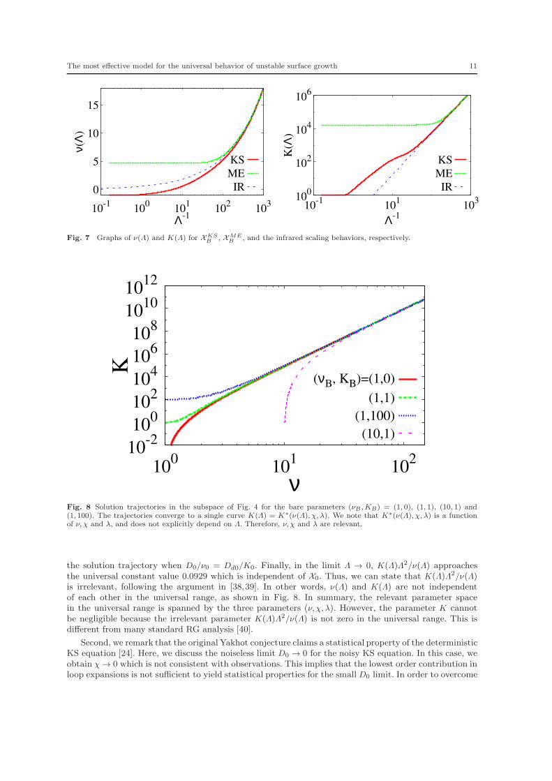
Fig. 8 Solution trajectories in the subspace of Fig. 4 for the bare parameters (νB ,KB) = (1, 0), (1, 1), (10, 1) and(1, 100). The trajectories converge to a single curve K(Λ) = K∗(ν(Λ), χ, λ). We note that K∗(ν(Λ), χ, λ) is a functionof ν, χ and λ, and does not explicitly depend on Λ. Therefore, ν, χ and λ are relevant.

the solution trajectory when D0/ν0 = Dd0/K0. Finally, in the limit Λ → 0, K(Λ)Λ2/ν(Λ) approachesthe universal constant value 0.0929 which is independent of X0. Thus, we can state that K(Λ)Λ2/ν(Λ)is irrelevant, following the argument in [38,39]. In other words, ν(Λ) and K(Λ) are not independentof each other in the universal range, as shown in Fig. 8. In summary, the relevant parameter spacein the universal range is spanned by the three parameters (ν, χ, λ). However, the parameter K cannotbe negligible because the irrelevant parameter K(Λ)Λ2/ν(Λ) is not zero in the universal range. This isdifferent from many standard RG analysis [40].

Second, we remark that the original Yakhot conjecture claims a statistical property of the deterministicKS equation [24]. Here, we discuss the noiseless limit D0 → 0 for the noisy KS equation. In this case, weobtain χ → 0 which is not consistent with observations. This implies that the lowest order contribution inloop expansions is not sufficient to yield statistical properties for the small D0 limit. In order to overcome


this situation, we have to formulate a non-perturbative calculation. This is an interesting problem forfuture work.

Finally, we expect that the concept proposed in this paper will be applied to various systems, althoughwe have studied a specific phenomenon as an example of scale-dependent parameters. The most interestingexample may be fluid turbulence. The effective model for the universal range in the turbulence is givenby a noisy Navier-Stokes equation [5,6,7,8,9,10,11]

∂tv(x, t) = −∇p(x, t) + η0∇2v(x, t) + f(x, t), (64)

〈fi(x, t)fj(x′

, t′

)〉 = 2Pij(∇)F (x− x′

)δ(t− t′

), (65)

where v is the fluid velocity, p is the pressure, η0 is the viscosity and f is the noise. Here, Pij and F inthe Fourier space are given as

Pij(k) = δij −kikjk2

, (66)

F (k) = (2π)d2D0k−y, (67)

where d is the space dimension, D0 is the noise strength, and y is a positive parameter. When y = d = 3,this model exhibits the Kolmogorov scaling law

E(k) = Ck−5/3, (68)

where E(k) is the energy spectra and C is a universal constant and takes the value ∼ 1.5. The analysisof solution trajectories of an RG equation for such the noisy Navier-Stokes equation may provide freshinsight into the understanding of the turbulence such as the universal constant C. We hope that thispaper stimulates the study of whole solutions of RG equations in various research fields.

The authors thank K. A. Takeuchi, M. Itami, and T. Haga for useful discussions. The present studywas supported by KAKENHI (Nos. 25103002 and 17H01148).

References

1. U. Frisch, Turbulence, (Cambridge University Press, Cambridge, 1995).2. L. F. Richardson, Proc. R. Soc. Lond. A. 110, 709-737 (1926).3. Y. Pomeau and P. Resibois, Phys. Rep. 19C 64 (1975).4. D. Forster, D. R. Nelson, and M. J. Stephen Phys. Rev. A 16, 732 (1977).5. C. DeDominicis and P. C. Martin, Phys. Rev. A. 19, 419-421 (1979)6. J. D. Fournier and U. Frisch, Phys. Rev. A 17, 747 (1978).7. J. D. Fournier and U. Frisch, Phys. Rev. A 28, 1000 (1983).8. V. Yakhot and S. A. Orszag, Phys. Rev. Lett. 57, 1722 (1986).9. V. Yakhot and S. Orszag, J. Sci. Comput. 1, 3 (1986).

10. V. Yakhot and M. L. Smith, J. Sci. Comput. 7, 35 (1992).11. G. L. Eyink, Phys. Fluids 6 3063 (1994).12. M. Kardar, G. Parisi, and Y.-C.Zhang, Phys. Rev. Lett. 56, 889 (1986).13. L. Bertini and G. Giacomin, Comm. Math. Phys. 183, 571 (1997).14. T. Sasamoto and H. Spohn, Phys. Rev. Lett. 104, 230602 (2010).15. K. A. Takeuchi and M. Sano, Phys. Rev. Lett. 104, 230601 (2010).16. K. A. Takeuchi, M. Sano, T. Sasamoto and H. Spohn, Sci. Rep. 1, 34 (2011).17. G. Amir, I. Corwin, and J. Quastel, Comm. Pure Appl. Math. 64 466 (2010).18. P. Calabrese and P. LeDoussal, Phys. Rev. Lett. 106, 250603 (2011).19. T. Imamura and T. Sasamoto Phys. Rev. Lett. 108, 190603 (2012).20. M. Hairer, Annals of Mathematics 178 559, (2013).21. Y. Kuramoto and T. Tsuzuki, Prog. Theor. Phys. 55, 356 (1976).22. G. I. Sivashinsky, Acta Astron. 4, 1177 (1977).23. Y. Kuramoto, Chemical Oscillations, Waves, and Turbulence, (Springer, Berlin, 1984).24. V. Yakhot, Phys. Rev. A 24, 642 (1981).25. V. Yakhot and Z.-S. She, Phys. Rev. Lett. 60, 1840 (1988).26. S. Zaleski, Physica D 34, 427 (1989).27. K. Sneppen, J. Krug, M. H. Jensen, C. Jayaprakash, and T. Bohr, Phys. Rev. A 46, R7351 (1992).28. F. Hayot, C. Jayaprakash, and C. Josserand, Phys. Rev. E 47, 911 (1993).29. H. Sakaguchi, Prog. Theor. Phys. 107, 879 (2002).30. K. Ueno, H. Sakaguchi, and M. Okamura, Phys. Rev. E 71, 046138 (2005).31. R. Cuerno and K. B. Lauritsen, Phys. Rev. E 52, 4853 (1995).32. P. C. Martin, E. D. Siggia, and H. A. Rose, Phys. Rev. A 8, 423 (1973).


33. H. K. Janssen, Z. Phys. B 23, 377 (1976).34. C. De Dominicis, J. Phys. Colloq. 37, C1-247 (1976).35. C. De Dominicis, Phys. Rev. B 18, 4913 (1978).36. E. Frey and U. C. Tauber, Phys. Rev. E 50, 1024 (1994).37. L. Canet, H. Chate, B. Delamotte, and N. Wschebor, Phys. Rev. E 84, 061128 (2011).38. J. Polchinski, Nucl. Phys. B 231, 269 (1984).39. S. Weinberg, The quantum theory of fields, (Cambridge university press, Cambridge, 1995).40. K. G. Wilson and J. Kogut, Phys. Rep. 12, 75 (1974).

A Ward-Takahashi identities

In this section, we proveλ(Λ) = λ0, (69)

for all generalized KPZ equations, andν(Λ)

D(Λ)=

ν0

D0

, (70)

for K0 = Dd0 = 0 or K0/Dd0 = ν0/D0, andK(Λ)

Dd(Λ)=

ν0

D0

, (71)

for K0/Dd0 = ν0/D0. These results are easily obtained from the following Ward-Takahashi identities [36,37]:

(G−1)hh(k = 0, ω;Λ) = −iω, (72)

iλ0k1∂ω1(G−1)hh(k1, ω1;Λ) = lim

ω,k→0∂kΓhhh(k1, ω1; k, ω;Λ), (73)

and

G−1

hh(k1, ω1;Λ) +G−1

hh(−k1,−ω1;Λ) = −

ν0k21D0

G−1

hh(k1,−ω1;Λ). (74)

These identities are relaed to invariance properties of the MSRJD action for a shift transformation, a tilt transformation,and a time-reversal transformation, respectively. In the next subsections, we will derive (72)-(74) following the arguments[36,37].

Here, we derive (69)-(71) from (72)-(74). First, by differentiating (73) with respect to k1 and taking the limit k1 → 0,we have

iλ0∂ω1(G−1)hh(k1 = 0, ω1;Λ) = lim

ω,k,k1→0∂k∂k1

Γhhh(k1, ω1; k, ω;Λ). (75)

Next, we substitute (72) to (75) and take the limit ω1 → 0. Then, we obtain

λ0 = limω,ω1,k,k1→0

∂k∂k1Γhhh(k1, ω1; k, ω;Λ). (76)

By recalling the definition (19), we find that this equality is (69). Second, we differentiate (74) twice with respect to k1.Then, we have

∂2k1

G−1

hh(k1, ω1;Λ) + ∂2

k1G−1

hh(−k1,−ω1;Λ) = −

ν0

D0

(2 + 2k1∂k1+ k21∂

2k1

)G−1

hh(k1,−ω1;Λ). (77)

By taking the limit ω1, k1 → 0 and using (15) and (17), we obtain (70). Finally, by differentiating (74) four times withrespect to k1, we arrive at (71).

A.1 Proof of (72)

We consider a shift transformation

h′

(x, t) = h(x, t) + c(t), (78)

where c(t) is an infinitesimal parameter that depends on time. The variation of the MSRJD action for the transformationis calculated as

S[h′

, ih′

;Λ0]− S[h, ih;Λ0] =

∫

dtdxih(x, t)∂tc(t). (79)


It should be noted that this simple form comes from the invariance property of the MSRJD action for the time-independent c 1. Then, the variation of the effective MSRJD action is derived as

S[h<′

, ih′<;Λ] =− log

∫

D[h>′

, ih>′

] exp

[

−S[h′

, ih′

;Λ0]

]

,

=− log

∫

D[h>, ih>] exp

[

−S[h, ih;Λ0]−

∫

dtdxih(x, t)∂tc(t)

]

,

=

∫

dtdxih<(x, t)∂tc(t) − log

∫

D[h>, ih>] exp

[

−S[h, ih;Λ0]−

∫

dtdxih>(x, t)∂tc(t)

]

,

=S[h<, ih<;Λ] +

∫

dtdxih<(x, t)∂tc(t). (80)

When we obtain the fourth line in (80) from the third line, we have used

∫

dtdxih>(x, t)∂tc(t) =

∫

dt∂tc(t)

(∫

dxih>(x, t)

)

,

=

∫

dt∂tc(t)ih>(k = 0, t),

= 0. (81)

Here, noting the trivial relation

S[h<′

, ih′<;Λ] = S[h<, ih<;Λ] +

∫

dtdxδS[h<, ih<;Λ]

δh<(x, t)c(t), (82)

we rewrite (80) as

∫

dtdx

(

δS[h<, ih<;Λ]

δh<(x, t)c(t)− ih<(x, t)∂tc(t)

)

= 0, (83)

which is further expressed as

∫

dtdx

(

δS[h<, ih<;Λ]

δh<(x, t)+ ∂tih

<(x, t)

)

c(t) = 0. (84)

Since this equality holds for any c(t), we obtain

∫

dx

(

δS[h<, ih<;Λ]

δh<(x, t)+ ∂tih

<(x, t)

)

= 0. (85)

The differentiation of (85) with respect to ih<(t′

, x′

) leads to

∫

dx

(

(G−1)hh(x′

− x, t′

− t;Λ) + ∂tδ(t − t′

)δ(x − x′

)

)

= 0. (86)

By performing the Fourier transformation, we arrive at (72).

A.2 Proof of (73)

We consider a tilt transformation

h′

(x, t) = h(x+ λ0vt, t) + vx, (87)

h′

(x, t) = h(x+ λ0vt, t), (88)

where v is an infinitesimal parameter. The tilt transformation for their Fourier transforms is expressed as

h′

(k, t) = eiλ0vkth(k, t)− iv∂kδ(k), (89)

ih′

(k, t) = eiλ0vkth(k, t). (90)

1 In general, by assuming time dependence of the infinitesimal parameter for a continuous symmetry transformation,we can obtain non-trivial identities such as (72). This technique, which has been referred to as “gauging a globalsymmetry”, is standard when we derive identities from a continuous global symmetry [39]. For such a case, the variationof an action under a time-gauged transformation is expressed as δS =

∫

dtQ(t)∂tǫ(t), where Q(t) is a Noether charge ofthe corresponding global symmetry, and ǫ(t) is the time-gauged infinitesimal parameter. The Noether charge of the shift

symmetry is calculated as Qshift =∫

dxih(x, t), which is consistent with (79).


We then find the symmetry property

S[h<′

+ h>′

, ih<′

+ ih>′

;Λ0] = S[h< + h>, ih< + ih>;Λ0], (91)

from which we obtain

S[h<, ih<;Λ] = − log

∫

D[h>, ih>] exp

[

−S[h< + h>, ih< + ih>;Λ0]

]

,

= − log

∫

JD[h>′

, ih>′

] exp[−S

[

h<′

+ h>′

, ih<′

+ ih>′

;Λ0]

]

,

= S[h<′

, ih<′

;Λ]− logJ , (92)

where J = 1 + va is the Jacobian for the tilt transformation, and a is a field independent quantity. The expansion of(92) in v leads to the identity

∫

dkdt

[

iλ0kt

(

δS[h<, ih<;Λ]

δh<(k, t)h<(k, t) +

δS[h<, ih<;Λ]

δih<(k, t)ih<(k, t)

)

+ iδ(k)∂kδS[h<, ih<;Λ]

δh<(k, t)− a

]

= 0. (93)

We differentiate this identity with respect to ih<(k1, t1) and h<(k2, t2). Then, we have

∫

dkdt

[

iλ0kt

(

δ2S[h<, ih<;Λ]

δh<(k, t)δih<(k1, t1)δ(k2 − k)δ(t2 − t) +

δ3S[h<, ih<;Λ]

δh<(k, t)δih<(k1, t1)δh<(k2, t2)h<(k, t)

+δ2S[h<, ih<;Λ]

δih<(k, t)δh<(k2, t2)δ(k1 − k)δ(t1 − t) +

δ3S[h<, ih<;Λ]

δh<(k, t)δih<(k1, t1)δh<(k2, t2)ih<(k, t)

)

+ iδ(k)∂kδ3S[h<, ih<;Λ]

δh<(k, t)δih<(k1, t1)δh<(k2, t2)

]

= 0. (94)

By taking the limit ih<, h< → 0 and recalling the definitions given in (12) - (14), we obtain

λ0(k1t1 + k2t2)(G−1)hh(k1, t1 − t2;Λ)δ(k1 + k2)

= −i limk→0

∂k

∫

dtΓhhh(k, k1, k2; t− t1, t2 − t1;Λ)δ(k + k1 + k2). (95)

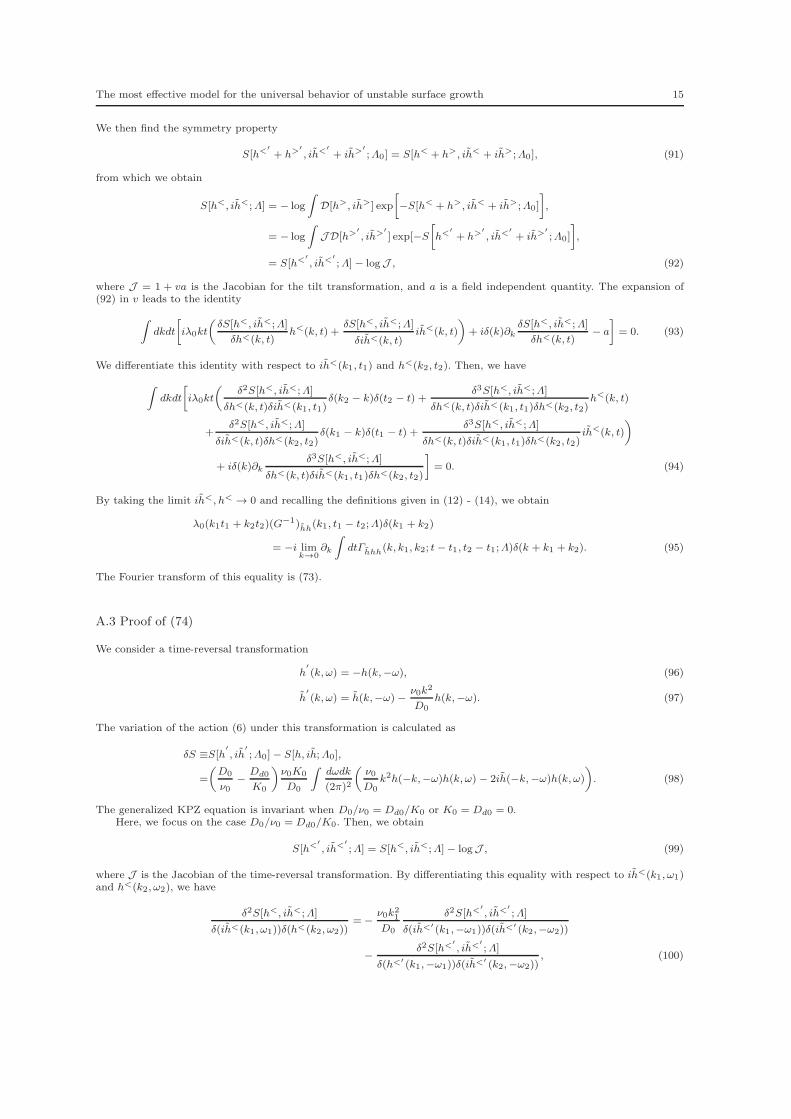
The Fourier transform of this equality is (73).

A.3 Proof of (74)

We consider a time-reversal transformation

h′

(k, ω) = −h(k,−ω), (96)

h′

(k, ω) = h(k,−ω)−ν0k2

D0

h(k,−ω). (97)

The variation of the action (6) under this transformation is calculated as

δS ≡S[h′

, ih′

;Λ0]− S[h, ih;Λ0],

=

(

D0

ν0−

Dd0

K0

)

ν0K0

D0

∫

dωdk

(2π)2

(

ν0

D0

k2h(−k,−ω)h(k, ω) − 2ih(−k,−ω)h(k, ω)

)

. (98)

The generalized KPZ equation is invariant when D0/ν0 = Dd0/K0 or K0 = Dd0 = 0.Here, we focus on the case D0/ν0 = Dd0/K0. Then, we obtain

S[h<′

, ih<′

;Λ] = S[h<, ih<;Λ]− logJ , (99)

where J is the Jacobian of the time-reversal transformation. By differentiating this equality with respect to ih<(k1, ω1)and h<(k2, ω2), we have

δ2S[h<, ih<;Λ]

δ(ih<(k1, ω1))δ(h<(k2, ω2))=−

ν0k21D0

δ2S[h<′

, ih<′

;Λ]

δ(ih<′ (k1,−ω1))δ(ih<′ (k2,−ω2))

−δ2S[h<′

, ih<′

;Λ]

δ(h<′ (k1,−ω1))δ(ih<′ (k2,−ω2)), (100)


where we have used the relation

δ

δh(k, ω)= −

δ

δh′ (k,−ω)−

ν0k2

D0

δ

δih′ (k,−ω), (101)

δ

δih(k, ω)=

δ

δih′ (k,−ω). (102)

By recalling the definition given in (12) - (14), we obtain

G−1

hh(k1, ω1;Λ)δ(ω1 + ω2)δ(k1 + k2)

=−

(

ν0k21D0

G−1

hh(k1,−ω1;Λ) +G−1

hh(−k1,−ω1;Λ)

)

δ(ω1 + ω2)δ(k1 + k2). (103)

By rearranging (103), we arrive at the identities (74).

Documents

Shin-ichi Sasa arXiv:1703.08946v2 [cond-mat.stat … · Yuki Minami · Shin-ichi Sasa September 13, 2017 Abstract We study a noisy Kuramoto-Sivashinsky (KS) equation which describes