ARTICLE IN PRESS

0165-1684/$ - se

doi:10.1016/j.sig

�CorrespondE-mail addre

Signal Processing 86 (2006) 1597–1603

www.elsevier.com/locate/sigpro

Shift, scaling and derivative properties for the discretecosine transform

Robert Reevesa,�, Kurt Kubikb

aSchool of Mathematical Sciences, Queensland University of Technology, GPO Box 2434, Brisbane, Q 4001, AustraliabSchool of Information Technology and Electrical Engineering, University of Queensland, Brisbane, Q 4072, Australia

Received 5 December 2002; accepted 5 September 2005

Available online 30 March 2006

Abstract

A set of DCT domain properties for shifting and scaling by real amounts, and taking linear operations such as

differentiation is described. The DCT coefficients of a sampled signal are subjected to a linear transform, which returns

the DCT coefficients of the shifted, scaled and/or differentiated signal. The properties are derived by considering the

inverse discrete transform as a cosine series expansion of the original continuous signal, assuming sampling in accordance

with the Nyquist criterion. This approach can be applied in the signal domain, to give, for example, DCT based

interpolation or derivatives. The same approach can be taken in decoding from the DCT to give, for example, derivatives

in the signal domain. The techniques may prove useful in compressed domain processing applications, and are interesting

because they allow operations from the continuous domain such as differentiation to be implemented in the discrete

domain. An image matching algorithm illustrates the use of the properties, with improvements in computation time and

matching quality.

r 2006 Elsevier B.V. All rights reserved.

Keywords: DCT; Image compression; Derivative; Shift; Scale; Image matching; JPEG

1. Introduction

The Discrete Cosine Transform (DCT) [1,2] hasfound wide application in image and video compres-sion, and continues to be at the center of innovativeresearch, with recent publications focussing oncomputation speed (e.g. [3,4], and transform domainfiltering (e.g. [5]). In this paper, a novel interpretationof the DCT is presented, which allows someinteresting properties to be derived. These properties

e front matter r 2006 Elsevier B.V. All rights reserved

pro.2005.09.041

ing author.

ss: r.reeves@qut.edu.au (R. Reeves).

include ways to generate the DCT of shifted, scaledor differentiated versions of a signal, directly from itsDCT coefficients. The method is based on interpret-ing the DCT coefficients as the coefficients of a cosineseries expansion of a band-limited, symmetricallyextended continuous signal. Similar approachesbased on splines and polynomial bases have beenreported [6,7]. In Section 2 we establish the validity oftreating the DCT as a sum of continuous sinusoidalbases. In Section 3, we use this interpretation toderive properties for DCT domain shifting, scalingand differentiation, and in Section 4, we illustrate theuse of the properties in an image matching algorithm.

.

ARTICLE IN PRESSR. Reeves, K. Kubik / Signal Processing 86 (2006) 1597–16031598

2. DCT as sum of continuous basis functions

Usually, the DCT is interpreted as a sum ofdiscrete bases, summing to a discrete sequence. Inthis section we interpret the DCT as a sum ofcontinuous bases. These bases sum to the symme-trically extended, band-limited continuous signal,which when sampled, gives rise to the discretesequence referred to above.

Let gðxÞ be a band limited continuous signal, suchthat omaxop. Without loss of generality, a samplinginterval of one is used, producing N samples gðnÞ atn ¼ 0; . . . ;N � 1. The forward discrete transformand its inverse are defined as

GðmÞ ¼ TfgðnÞg ¼XN�1n¼0

gðnÞf nðmÞ (1)

and

gðnÞ ¼ T�1fGðmÞg ¼XN�1m¼0

GðmÞrmðnÞ, (2)

where f nðmÞ is the forward transform kernel, rmðnÞ isthe reverse transform kernel, and n and m areintegers from 0 to N � 1. The type-2 DCT [8], asused in the JPEG [1] and related compressionschemes is defined by

f nðmÞ ¼ rmðnÞ ¼ cðmÞ

ffiffiffi2p

ffiffiffiffiffiNp cosðð2nþ 1Þmp=2NÞ,

(3)

with cðmÞ ¼ 1=ffiffiffi2p

for m ¼ 0 and cðmÞ ¼ 1 other-wise, and gðxÞ is assumed to be symmetricallyextended with period 2N, so that gðxÞ ¼ gðxþ 2NÞ

and gð�ð1=2Þ þ xÞ ¼ gð�ð1=2Þ � xÞ.Though rmðnÞ is defined only for integer values

of n, the expression can be computed for any realvalue. Replacing the discrete n by real x gives a sumof continuous cosine basis functions,

gðxÞ ¼XN�1m¼0

rmðxÞGðmÞ. (4)

By considering the periodicity of the bases rmðxÞ andthe orthonormality of the DCT kernel, it is evidentthat when gðxÞ is sampled with an interval of one,the values gðnÞ and their symmetric and periodic

repetitions result, as follows:

gðxÞ ¼XN�1m¼0

rmðxÞXN�1n¼0

gðnÞf nðmÞ ð5Þ

¼XN�1n¼0

gðnÞXN�1m¼0

rmðxÞf nðmÞ. ð6Þ

Taking samples at values of x ¼ p, where p is aninteger from 0 to N � 1, and noting that f nðmÞ ¼

rmðnÞ we have

gðpÞ ¼XN�1n¼0

gðnÞXN�1m¼0

rmðpÞf nðmÞ ð7Þ

¼XN�1n¼0

gðnÞXN�1m¼0

f pðmÞf nðmÞ. ð8Þ

By orthonormality of the DCT kernel,PN�1m¼0 f pðmÞf nðmÞ is equal to zero unless p ¼ n,

and one otherwise. Thus sampling gðpÞ produces thesame samples gðnÞ as sampling gðxÞ. This is sufficientto imply the equivalence of these two signals, aslong as gðxÞ is sampled in accordance with theNyquist criterion. It is trivial to extend thisargument to those values of p outside the range 0to N � 1 by considering the periodic and symmetricextensions of rmðpÞ: rmðpÞ ¼ rmðpþ 2NÞ, andrmðpÞ ¼ rmð�1� pÞ.

3. DCT domain properties

In this section simple expressions are derived forcomputing the DCT of any linear operation on asignal, from the DCT coefficients of the originalsignal’s samples. Applying a linear operation toboth sides of (4), and adopting the notation gLðnÞ tomean the linearly transformed signal sampled atx ¼ n, and rLmðnÞ to refer to the linearly trans-formed kernel sampled at x ¼ n,

gLðnÞ ¼XN�1m¼0

GðmÞrLmðnÞ. (9)

It follows from (1) and (9) that

TfgLðnÞgðmÞ ¼XN�1p¼0

GðpÞXN�1n¼0

f nðmÞrLpðnÞ. (10)

This represents a linear transform which computesthe DCT of gLðnÞ from the DCT of gðnÞ, in a singlematrix multiplication. The values of the termsPN�1

n¼0 f nðmÞrLpðnÞ are independent of the signaland its samples, depending only on the type oflinear transformation.

ARTICLE IN PRESSR. Reeves, K. Kubik / Signal Processing 86 (2006) 1597–1603 1599

Differentiation is one example of a linearproperty that can be performed in the DCT domain.In this case gLðnÞ denotes the derivative of gðxÞ

sampled at x ¼ n, and

rLpðnÞ ¼ �cðpÞ

ffiffiffi2p

ffiffiffiffiffiNp

mpN

sinðð2nþ 1Þpp=2NÞ, (11)

given by the derivative of the reverse transformkernel, sampled at x ¼ n. The extension to secondand higher derivatives, real valued shift, scaling,integrals, or any combination of them, is trivial. Forexample, a shifting and scaling property is given byletting rLpðnÞ ¼ rpða0 þ a1nÞ.

4. Example—image matching

As an example of how these DCT properties canbe used, two-dimensional versions were incorpo-rated into an image matching algorithm based on

A ¼

..

. ... ..

. ... ..

. ... ..

. ...

1 gð�Þqqx

gð�Þ xqqx

gð�Þ yqqx

gð�Þqqy

gð�Þ xqqy

gð�Þ yqqy

gð�Þ

..

. ... ..

. ... ..

. ... ..

. ...

2666664

3777775. (17)

the standard approach of Ackermann [9], in whichpartial derivatives are required. An affine transfor-mation models the transformation of left imagepatch to right image patch as follows:

g1ðx; yÞ ¼ h0 þ h1gða0 þ a1xþ a2y; b0 þ b1xþ b2yÞ

þ n1ðx; yÞ ð12Þ

and

g2ðx; yÞ ¼ gðx; yÞ þ n2ðx; yÞ, (13)

where g1ðx; yÞ and g2ðx; yÞ are the image patches tobe matched, h0 and h1 are radiometric transforma-tion parameters, ai and bi are geometric transforma-tion parameters, and n1ðx; yÞ and n2ðx; yÞ areGaussian noise.

Using Taylor’s theorem to linearize each equationabout an initial guess and then subtracting yields

Dgðx; yÞ ¼ dh0 þ dh1gðx; yÞ þ da0qqx

gðx; yÞ

þ da1xqqx

gðx; yÞ þ da2yqqx

gðx; yÞ

þ db0qqy

gðx; yÞ þ db1xqqy

gðx; yÞ

þ db2yqqy

gðx; yÞ þ vðx; yÞ, ð14Þ

where x and y take on a series of discrete valueswithin a match window. This results in a system ofequations for the perturbations to the initial radio-metric and geometric transformation parameters.

The system of equations can be expressed inmatrix form

L ¼ Axþ v, (15)

with the solution given by

x ¼ ðATAÞ�1ATL, (16)

where x is the vector of perturbations to the initiallychosen transformation parameters that result in abetter match between the two image patches. Vectorv is a vector of noise terms, and A is given by

Since the solution is based around a linearapproximation, it can be improved by linearizingaround the new solution, and re-solving. This isrepeated until the solution converges.

By choosing a suitable ordering system, theimages can be expressed as column vectors, the 2Dlinear transform as a matrix, and (15) can beexpressed in the transform domain as

TAxþ Tv ¼ TL, (18)

where multiplying by matrix T takes the 2D DCTtransform. This can be viewed as defining transformdomain A and L matrices given by TA and TL. Ithas been shown previously that as long as T isorthogonal, which is the case for the DCT, thesolution of (16) is unaffected by using the transformdomain A and L matrices [10]. For typical images,the DCT behaves in a similar manner to theKarhunen–Loeve transform, which constructsbasis functions in order of decreasing variance. Inimage compression, this fact is used to justifydiscarding many of the high frequency (low

ARTICLE IN PRESS

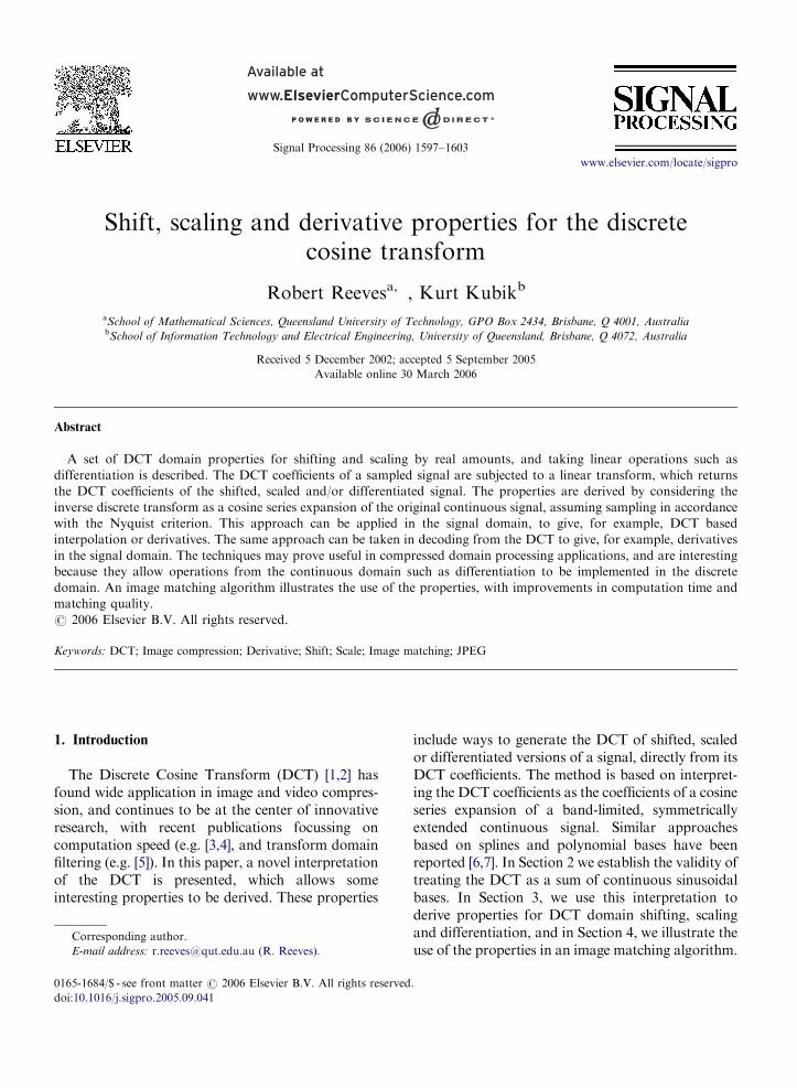
Fig. 1. Image one was formed by subsampling a 1600 � 1600

fragment using a 10� 10 Gaussian window, while the right image

was formed by first shifting by 5 pixels, then subsampling.

R. Reeves, K. Kubik / Signal Processing 86 (2006) 1597–16031600

variance) coefficients, while maintaining the infor-mation important to the structure of the image [11].This same principle can be extended to imagematching. Since the bulk of the image energyappears in the low order DCT coefficients, discard-ing the higher order coefficients should not impairimage matching. We can significantly reduce the sizeof the A matrix by transforming each column intothe DCT domain, and then omitting the same highfrequency coefficients from each column. Since thecomputational effort in the solution of the leastsquares system depends on the size of matrix ATA,this should enable the solution to be computed morequickly, without detriment to the quality of thematch result. The method of (10) is used to computethe transforms of the columns of the A matrixinvolving partial derivatives, from the transform ofthe image patch. The extension to two dimensions isstraightforward, with full details given in [12]. Anexperimental investigation is fully reported else-where [12,13]. Here we briefly summarise the mainresults concerning accuracy and computation time,when compared to a fully pixel domain algorithm inwhich the partial derivatives are estimated by firstdifferences.

It is important to note that as far as thisapplication is concerned, the important point thatresults in computational efficiencies is that the leastsquares problem (18) is solved in the transformdomain after removing those transform domainequations which effectively involve only noise. Whilewe have found it expedient to use the transformdomain properties we have proposed to compute thetransforms of the rows of A which involve partialderivatives from the transform of the image patch,an equivalent procedure would be to first computethe columns of A, finding the partial derivatives bysome other means, and then taking the DCT of eachcolumn of A. However, this introduces the problemof estimating the partial derivatives. Apart from theissues of the assumed periodic extension, and thesatisfaction of the Nyquist criterion, the partialderivatives involved in the methods we propose arethose of the original continuous function, notdiscrete estimates with an associated imprecision.As we discuss in Section 4.3 analogous properties inthe time(space) domain can be used to estimate thecolumns of A. However, in this case we would havean additional DCT to perform for each column of Ainvolving a partial derivative.

An artificial horizontal disparity was introducedinto two fragments of aerial photographs as follows.

In image one (Fig. 1), the left image was formed bysubsampling a 1600� 1600 fragment using a 10�10 Gaussian window, while the right image wasformed by first shifting by 5 pixels, then subsam-pling. In image two (Fig. 2), the left image wasformed by subsampling a 328� 328 fragment usinga 2� 2 Gaussian window, while the right image wasformed by first shifting by 1 pixel, then subsam-pling. This resulted in a known disparity of 0.5pixels being introduced in each case between the leftand right images.

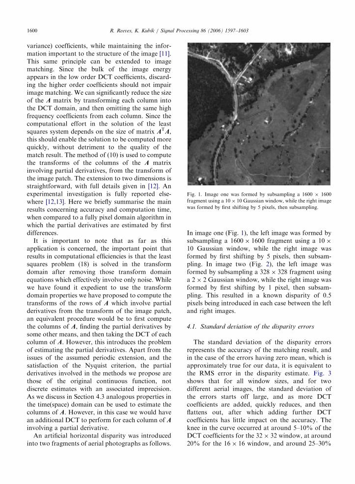
4.1. Standard deviation of the disparity errors

The standard deviation of the disparity errorsrepresents the accuracy of the matching result, andin the case of the errors having zero mean, which isapproximately true for our data, it is equivalent tothe RMS error in the disparity estimate. Fig. 3shows that for all window sizes, and for twodifferent aerial images, the standard deviation ofthe errors starts off large, and as more DCTcoefficients are added, quickly reduces, and thenflattens out, after which adding further DCTcoefficients has little impact on the accuracy. Theknee in the curve occurred at around 5–10% of theDCT coefficients for the 32� 32 window, at around20% for the 16� 16 window, and around 25–30%

ARTICLE IN PRESS

0 10 20 30 40 50 60 70 80 90 1000

0.1

0.2

0.3

0.4

0.5

0.6

0.7

0.8Standard Deviation of Disparity Error for Converged Match Windows

Percentage of DCT Coefficients Taken in Least Squares Adjustment

Sta

ndar

d D

evia

tion

of D

ispa

rity

Err

or (

pixe

ls)

8×8 - TD6×6 -PD16×16 - TD14×14 - PD32×32 - TD30×30 - PD

0 10 20 30 40 50 60 70 80 90 1000

0.2

0.4

0.6

0.8

1

1.2

1.4Standard Deviation of Disparity Error for Converged Match Windows

Percentage of DCT Coefficients Taken in Least Squares Adjustment

Sta

ndar

d D

evia

tion

of D

ispa

rity

Err

or (

pixe

ls)

8×8 - TD6×6 -PD16×16 - TD14×14 - PD32×32 - TD30×30 - PD

Fig. 3. Optimum matching accuracy is shown to be achieved with

a small percentage of the available DCT coefficients. Results are

shown for 8� 8, 16� 16 and 32� 32 windows for image one

(top) and image two (bottom). The accuracy achieved by a

comparable pixel domain algorithm are shown as dotted lines for

each of three window sizes.

Fig. 2. Image two was formed by subsampling a 328� 328

fragment using a 2� 2 Gaussian window, while the right image

was formed by first shifting by 1 pixel, then subsampling.

R. Reeves, K. Kubik / Signal Processing 86 (2006) 1597–1603 1601

for the 8� 8 window. In all cases, after the knee, theaccuracy was comparable or better than thatachieved by the pixel domain algorithm, sometimesmarkedly so.

4.2. Average convergence time

The average time for match windows to convergeis shown in Fig. 4. For the 8� 8 window, the timesfor the DCT domain algorithm are comparable tothe pixel domain for DCT coefficient percentages upto about 30%, but then gradually increase as furtherDCT coefficients are added. For the 16� 16window, taking between 10% and 30% of thecoefficients resulted in reducing the average con-vergence time to about 50% of the pixel domaintime in one image, and about 75% in the otherimage. The improvements were more pronouncedfor the 32� 32 window, where in both images theaverage convergence time was under 50% of thepixel domain time, when between 5% and 20% ofthe DCT coefficients were taken.

4.3. Discussion

From our use of these DCT domain properties,several important considerations emerge. Firstly,the properties are based on the assumption that thesignal is symmetrically extended at each end of the

DCT window [14], or block in the 2D case. Wherethe result of the linear operation is outside the DCTwindow (as possible with shifting or scaling), a pointon the symmetrically extended waveform is re-turned. In the case of the DCT support being theentire signal or image, this may be an acceptableedge effect. However, in block based decomposi-tions, edge effects may be introduced into eachblock. The symmetric extension also causes thederivative to tend towards zero at the edges of theDCT window. This may also be problematic inblock based schemas.

ARTICLE IN PRESS

0 10 20 30 40 50 60 70 80 90 1000

100

200

300

400

500

600

700

800

900

1000Average Match Time for Converged Match Windows

Percentage of DCT Coefficients Taken in Least Squares Adjustment

Tim

e (M

illi-s

econ

ds)

0 10 20 30 40 50 60 70 80 90 1000

100

200

300

400

500

600

700

800Average Match Time for Converged Match Windows

Percentage of DCT Coefficients Taken in Least Squares Adjustment

Tim

e (M

illi-s

econ

ds)

8×8 - TD6×6 -PD16×16 - TD14×14 - PD32×32 - TD30×30 - PD

8×8 - TD6×6 -PD16×16 - TD14×14 - PD32×32 - TD30×30 - PD

Fig. 4. The effect of taking only a fraction of the available DCT

coefficients in each least squares adjustment on the average time

taken to converge for each match window is shown for image one

(top) and image two (bottom). The times for the pixel domain

algorithms are shown as dotted horizontal lines for comparison.

R. Reeves, K. Kubik / Signal Processing 86 (2006) 1597–16031602

Time (space) domain versions of the propertyprovide a means of shifting, scaling and taking thederivative of sampled signals. For example, a shiftedsignal can be computed by

gðnþ aÞ ¼XN�1n¼0

gðnÞXN�1m¼0

f nðmÞrmðnþ aÞ. (19)

This equation represents a linear transform, basedon the DCT kernels and the shift parameter. Notethat the shift parameter a can be any real value. Thisequation can also be viewed as an interpolationfunction. Such an interpolation can be combinedwith scaling and taking the derivative. It differs

from a DCT interpolation technique proposed byWang [15–17] which results in an increased numberof samples, spanning the same signal support. In themethod proposed here, the number of samplesremains fixed, but the signal support may change ifscaling or shifting is involved.

The property can also be incorporated directlyinto the decoding step by making use of (9).

5. Summary and conclusions

Shift, scale and derivative properties for the DCTcan be derived by treating the inverse transform as asum of continuous cosine bases. This sum ofcontinuous bases is identical to the original con-tinuous signal, subject to the Nyquist criterion andthe assumed symmetric periodic extension.

A single linear transform can be used to computethe DCT of the sampled derivative, from the DCTof the original signal. Linear transforms can also beconstructed for other linear operations, for exampleshifting and scaling. Any number of sequentiallyapplied linear operations may be combined into asingle linear transform, based on applying thecombined transform to the cosine bases.

The property described in this paper may also beapplied in the time or space domain, for example, toshift a signal by a real (possibly fractional) numberof samples, or to differentiate it. Given that the 2DDCT is separable, there is no impediment to astraightforward 2D extension, which has been usedin a DCT domain image matching algorithm. Weexpect therefore that these techniques may be usefulfor DCT based image representations, particularlywhere geometric transformations or derivatives arerequired.

As an example of how these properties may beused, a standard least squares image matchingalgorithm was implemented in the DCT domain,making use of the properties described. The algo-rithm was able to perform more accurately andconverge faster than a comparable pixel domainalgorithm using first differences to estimate thepartial derivatives. This improved performance maybe attributed to two factors. Firstly, the DCTdomain algorithm enables us to discard a highpercentage of DCT coefficients in the least squaresadjustment, thus reducing the size of the solutionwithout losing significant image information. Sec-ondly, the DCT properties described provide abetter estimate of the partial derivatives than thefirst differences.

ARTICLE IN PRESSR. Reeves, K. Kubik / Signal Processing 86 (2006) 1597–1603 1603

References

[1] G.K. Wallace, The JPEG still-picture compression standard,

Comm. ACM 34 (4) (1991) 31–44.

[2] K.-H. Tzou, Video Coding Techniques: An Overview, in:

P. Pirsch (Ed.), VLSI Implementations for Image Commu-

nications, Elsevier Science Publishers, Amsterdam, 1993,

pp. 1–47.

[3] S. Lee, Improved algorithm for efficient computation of the

forward and backward MDCT in MPEG audio coder, IEEE

Trans. Circuits Syst. II—Analog Digital Signal Process. 48

(10) (2001) 990–994.

[4] J. Liang, T. Tran, Fast multiplierless approximations of the

DCT with the lifting scheme, IEEE Trans. Signal Process. 49

(12) (2001) 3032–3044.

[5] N. Nikolaev, A. Gotchev, K. Egiazarian, Z. Nikolov,

Suppression of electromyogram interference on the electro-

cardiogram by transform domain denoising, Medical Biolo-

gical Eng. Comput. 39 (6) (2001) 649–655.

[6] M. Unser, Splines—a perfect fit for signal and image

processing, IEEE Signal Process. Mag. 16 (6) (1999)

22–38.

[7] H. Ridha, J. Vesma, T. Saramaki, M. Renfors, Derivative

approximations for sampled signals based on polynomial

interpolation, in: Proceedings of the 13th International

Conference on Digital Signal Processing, vol. 2, IEEE,

New York, 1997, pp. 939–942.

[8] K. Rao, P. Yip, Discrete Cosine Transform—Algorithms,

Advantages, Applications, Academic Publishers, San Diego,

1990.

[9] F. Ackermann, Digital image correlation: performance and

potential application in photogrammetry, Photogramm.

Rec. 11 (64) (1984) 429–439.

[10] R. Reeves, K. Kubik, Least squares matching in the

transform domain, Internat. Arch. Photogramm. Remote

Sensing 32 (3/1) (1998) 168–176.

[11] M. Rabbini, P. Jones, Digital Image Compression Techni-

ques, SPIE Optical Engineering Press, Bellingham, WA,

1991.

[12] R. Reeves, Image matching in the compressed domain,

Ph.D. Thesis, Space Centre for Satellite Navigation, Queens-

land University of Technology, Brisbane, Australia, 1999.

[13] R. Reeves, K. Kubik, Benefits of hybrid DCT domain image

matching, Internat. Arch. Photogramm. Remote Sensing 32

(2000) 761–768.

[14] S.A. Martucci, Symmetric convolution and the discrete sine

and cosine transforms, IEEE Trans. Signal Process. 42 (5)

(1994) 1038–1051.

[15] Z. Wang, Interpolation using type I discrete cosine trans-

form, Electron. Lett. 26 (15) (1990) 1170–1171.

[16] Z. Wang, Interpolation using the discrete cosine transform:

reconsideration, Electron. Lett. 29 (2) (1993) 198–200.

[17] J. Agbinya, Two dimensional interpolation of real sequences

using the DCT, Electron. Lett. 29 (2) (1993) 204–205.