1

Shell Balances in Fluid Mechanics

R. Shankar Subramanian Department of Chemical and Biomolecular Engineering

Clarkson University When fluid flow occurs in a single direction everywhere in a system, shell balances are useful devices for applying the principle of conservation of momentum. An example is incompressible laminar flow of fluid in a straight circular pipe. Other examples include flow between two wide parallel plates or flow of a liquid film down an inclined plane. In the above situations, fluid velocity varies across the cross-section only in one coordinate direction and is uniform in the other direction normal to the flow direction. For flow through a straight circular tube, there is variation with the radial coordinate, but not with the polar angle. Similarly, for flow between wide parallel plates, the velocity varies with the distance coordinate between the two plates. If the plates are sufficiently wide, we can ignore variations in the other direction normal to the flow which runs parallel to the surfaces of the plates. If we neglect entrance and exit effects, the velocity does not vary with distance in the flow direction in both cases; this is the definition of fully-developed flow. A momentum balance can be written for a control volume called a shell, which is constructed by translating a differential cross-sectional area (normal to the flow) in the direction of the flow over a finite distance. The differential area itself is formed by taking a differential distance in the direction in which the velocity varies and translating it in the other cross-sectional coordinate over its full extent. We shall see by example how these shells are formed. The key idea is that we use a differential distance in the direction in which velocity varies. Later, we consider the limit as this distance approaches zero and obtain a differential equation. Typically this is an equation for the shear stress. By inserting a suitable rheological model connecting the shear stress to the velocity gradient, we can obtain a differential equation for the velocity distribution. This is then integrated with the boundary conditions relevant to the problem to obtain the velocity profile. Once the profile is known, we can calculate the volumetric flow rate and the average velocity as well as the maximum velocity. If desired, the shear stress distribution across the cross-section can be written as well. In the case of pipe flow, we shall see how this yields the well-known Hagen-Poiseuille equation connecting the pressure drop and the volumetric flow rate. Regarding boundary conditions, the most common condition we use is the “no slip” boundary condition. This states that the fluid adjacent to a solid surface assumes the velocity of the solid. Also, when necessary we use symmetry considerations to write boundary conditions. At a free liquid surface when flow is not driven by the adjoining gas dragging the liquid, we can set the shear stress to zero. In general at a fluid-fluid interface the velocity and the shear stress are continuous across the interface. Even though the interfacial region is made up of atoms and molecules and has a non-zero

2

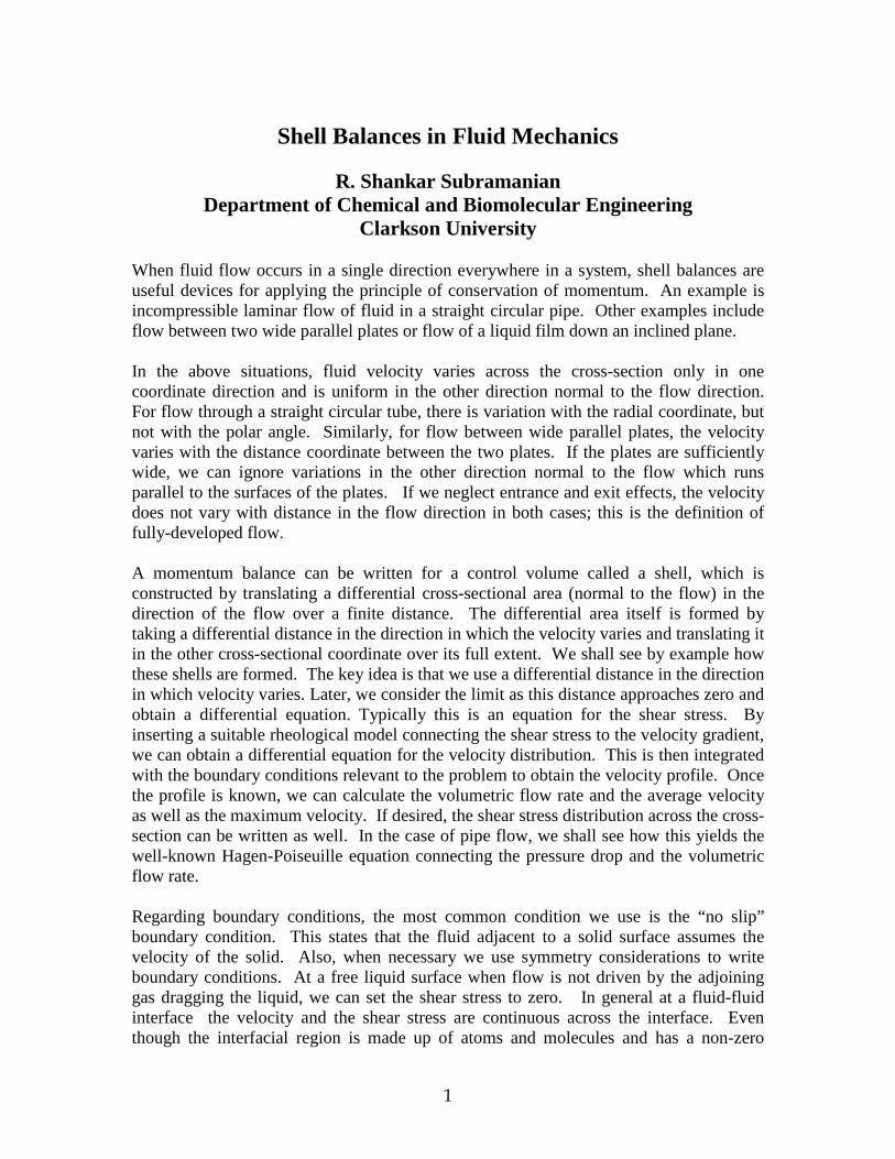
thickness, we treat is as a plane of zero thickness for this purpose. This means that the value of the velocity at a given point on the interface in one fluid is the same as the value of the velocity at the same point on the interface in the second fluid. The same is true of the shear stresses in the two fluids except when the interfacial tension varies with position. This can happen if the temperature varies along the surface or if surface active chemicals are present. Now, we shall proceed to construct a shell momentum balance for steady laminar flow through a straight circular tube. Steady Fully-Developed Incompressible Laminar Flow in a Straight Circular Tube Cylindrical polar coordinates ( ), ,r zφ are used. We assume steady incompressible fully-developed laminar flow in the z -direction. The only non-zero velocity component is zv and it only depends on the radial coordinate r . Therefore, ( )z zv v r= . Similarly, the

shear stress ( )rz rz rτ τ= . The shell shown in the figure is L units long and r∆ units thick in the radial direction. Its inner cylindrical surface is at a radial location r and the outer cylindrical surface is at r r+ ∆ . At steady state, the rate of accumulation of momentum in the fluid contained in the shell is zero. Momentum enters at the left face and leaves at the right face with the flowing fluid. The shell balance reads as follows. Rate of entry of momentum into shell - Rate of efflux of momentum from the shell + Sum of all the forces acting on the fluid in the shell = 0.

Flow Shellrz

r∆

L

θ

R

3

The volumetric flow rate of fluid into the shell is

2 zQ r r vπ∆ = ∆ If the density of the fluid is ρ , the associated mass flow rate into the shell is

[ ] 02 z z

m r r vπ ρ=

∆ = ∆ and the rate of entry of momentum, which is the product of the mass flow rate and the velocity, is written as follows. Rate of entry of momentum [ ] 2

0 02z zz z

m v r r vπ ρ= =

= ∆ = ∆

Similarly, the rate of efflux of momentum out of the right face can be written at Rate of efflux of momentum [ ] 22z zz L z L

m v r r vπ ρ= =

∆ = ∆

Because zv only depends on r and not on z , the two terms cancel each other. So the shell balance reduces to the statement that the sum of the forces on the fluid in the shell is zero. The forces on the fluid consist of the pressure force, the gravitational force, and the viscous force. We shall account for each in turn. The pressure force, given as the product of the area and the pressure acting on it, is written as follows. Pressure force ( ) ( )2 0r r p p Lπ= ∆ − The force of gravity on the fluid in the shell, given as the product of the mass of the fluid in the shell and the (vector) acceleration due to gravity g acts vertically downward. We need to use the component of this force in the z -direction. This can be obtained as Contribution in the flow direction from the gravitational force 2 cosr rL gπ ρ θ= ∆ where g is the magnitude of the (vector) acceleration due to gravity g . We now calculate the viscous force acting on the shell. The fluid at r r+ ∆ exerts a shear stress on the fluid in the shell in the positive z − direction which we designate as

( )rz r rτ + ∆ . This notation means “shear stress evaluated at the location r r+ ∆ .” Multiplied by the surface area of the shell at that location this yields a force

( ) ( )2 rzr r L r rπ τ+ ∆ + ∆ in the z − direction. In the same way, the fluid within the shell

4

at the location r exerts a stress ( )rz rτ on the fluid below, i.e. at smaller r . As a result, the fluid below exerts a reaction on the shell fluid that has the opposite sign. The resulting force is ( )2 rzrL rπ τ− . Therefore, the total force arising from the shear stresses on the two cylindrical surfaces of the shell fluid is written as follows. Force from viscous stress ( ) ( ) ( )2 rz rzL r r r r r rπ τ τ= + ∆ + ∆ − Add the forces, set the sum to zero, and divide by 2 rLπ∆ to obtain the following result.

( ) ( ) ( ) ( ) ( )0cos 0rz rzp p L r r r r r r

r gL r

τ τρ θ

− + ∆ + ∆ − + + = ∆

Now we take the limit of the terms in the above equation as 0r∆ → . The first term is unaffected while the second term is simply the derivative of rzrτ with respect to r . This leads us to the first order differential equation for the shear stress ( )rz rτ .

( )1rz

d Prr dr L

τ ∆= −

where we have introduced the symbol

( ) ( )0 cosP p p L gLρ θ∆ = − + for convenience. The quantity P is known as the hydrodynamic pressure or simply the dynamic pressure. Its gradient is zero in a stationary fluid and therefore it is uniform when the fluid is not in motion. We can integrate the differential equation for the shear stress immediately by noting that the right side is just a constant while the left side is the derivative of rzrτ . The result of this integration is

2

12rzP rr C

Lτ ∆

= − +

where 1C is an arbitrary constant of integration that needs to be determined. We can rewrite this result as

1

2rzCP r

L rτ ∆

= − +

5

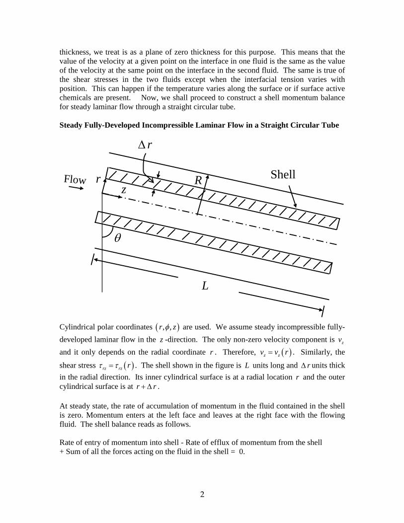
According to this result, the shear stress should approach infinity as the radial coordinate 0r → . This is not physically possible. Therefore, we must choose the arbitrary constant

of integration 1 0C = and write the shear stress distribution in the tube as follows.

2rzP rL

τ ∆= −

The shear stress is zero at the centerline and its magnitude is a maximum at the tube wall. It varies linearly across the cross-section. We can explain why it is negative. Recall that a force acting in the positive z − direction is taken by convention here to be positive. The fluid at the wall is stationary, however, and exerts a viscous force in the negative z −direction on fluid in the adjacent layer which is trying to slide past it. This is why the shear stress, according to our convention, is negative. A sketch of the shear stress distribution is given below. To find the velocity distribution, we need to introduce a relationship between the shear stress and the velocity gradient. Recall the Newtonian constitutive model

zrz

dvdr

τ µ=

where µ is the dynamic viscosity of the fluid. Use of this constitutive model in the result for the shear stress leads to

2zdv P r

dr Lµ∆

== −

rz

R

( )rz rτ

6

This equation can be integrated immediately to yield

( ) 22 4z

Pv r C rLµ

∆= −

where a new arbitrary constant of integration 2C has been introduced. To determine this constant we must impose a boundary condition on the velocity field. This is the no slip boundary condition at the tube wall r R= . ( ) 0zv R =

Use of this condition leads to the result

2

2 4P RC

Lµ∆

=

so that we can write the velocity distribution as follows.

( )2 2

214zP R rv r

L Rµ ∆

= −

This velocity distribution describes a parabola. It is sketched below. We see that the maximum velocity occurs at the centerline, which is at 0r = . Its value is

2

max 4P Rv

Lµ∆

=

rz R

( )zv r

7

We can calculate the volumetric flow rate through the tube by multiplying the velocity at a given r by the differential cross-sectional area 2 r drπ to yield dQ and then integrating across the cross-section.

( )2 2

20 0 0

4

2 12

8

Q R R

zP R rQ dQ r v r dr r drL R

P RL

ππµ

πµ

∆= = = −

∆

=

∫ ∫ ∫

This is a result known as the Hagen-Poiseuille equation for the relationship between the flow rate and the applied pressure drop for laminar flow through a circular tube. Now, we can calculate the average velocity in the tube, defined as the volumetric flow rate per unit area of cross-section.

It can be seen that in a circular tube, the average velocity is one-half the maximum velocity. Steady Fully-Developed Incompressible Laminar Flow Between Parallel Plates A similar development can be made for flow between wide parallel plates that are separated by a distance 2h . Let us consider flow driven by a pressure difference

( ) ( )0p p p L∆ = − between the inlet and exit of a channel formed two horizontal parallel plates.

zy

Hx

Shell

y∆

Flow

L

2

avg 2 8Q P RvR Lπ µ

∆= =

8

A sketch of the channel, showing a shell that is L units long and W units wide in the direction normal to the plane of the paper is shown. We make the following assumptions. Fully developed flow (Means no end effects) Steady flow Incompressible flow (means constant density) Newtonian flow Laminar flow The only non-zero velocity component is zv and it only depends on the coordinate y . Therefore, ( )z zv v y= . The thickness of the shell in the y −direction is y∆ . From the inlet, the end view of the shell looks like this.

Conservation of Momentum At steady state, the rate of accumulation of momentum in the fluid contained in the shell is zero. Momentum enters at the left face and leaves at the right face with the flowing fluid. The shell balance reads as follows. Rate of entry of momentum into shell - Rate of efflux of momentum from the shell + Sum of all the forces acting on the fluid in the shell = 0. Now, the volumetric flow rate of fluid into the shell is

[ ] 0z zQ W y v

=∆ = ∆ If the density of the fluid is ρ , the associated mass flow rate is

[ ] 0z zm W y vρ

=∆ = ∆ and the rate of entry of momentum, which is the product of the mass flow rate and the velocity, is written as follows. Rate of entry of momentum [ ] 2

0 0z zz zm v W y vρ

= = = ∆ = ∆

Similarly, the rate of efflux of momentum out of the right face can be written at

Wy∆

9

Rate of efflux of momentum [ ] 2z zz L z L

m v W y vρ= =

= ∆ = ∆

Because zv only depends on y and not on z , the two terms cancel each other. So the shell balance reduces to the statement that the sum of the forces on the fluid in the shell is zero. The forces on the fluid consist of the gravity force, the pressure force, and the viscous force. We shall account for each in turn. The force of gravity acts downward and makes no contribution to the momentum changes in the z − direction. Its main role is to produce a hydrostatic variation of pressure with height that can be taken out by redefining the pressure as the “hydrodynamic pressure,” which is uniform across the cross-section of the channel at any given z . The pressure force, given as the product of the area and the pressure acting on it, is written as follows. Pressure force ( ) ( )0W y p p L= ∆ − We now calculate the viscous force acting on the shell. The fluid at y y+ ∆ exerts a shear stress on the fluid in the shell in the positive z − direction, which we designate as

( )yz y yτ + ∆ . This notation means “shear stress evaluated at the location y y+ ∆ .”

Multiplied by the surface area of the shell, this yields a force ( )yzWL y yτ + ∆ in the z −direction. In the same way, the fluid within the shell at the location y exerts a stress

( )yz yτ on the fluid below, i.e. at smaller y . As a result, the fluid below exerts a reaction

on the shell fluid that has the opposite sign. The resulting force is ( )yzWL yτ− . Therefore, the total force arising from the shear stresses on the top and bottom surfaces of the shell fluid is written as follows. Force from viscous stress ( ) ( )yz yzWL y y yτ τ = + ∆ − Add the forces and set the sum to zero.

( ) ( ) ( ) ( )0 0yz yzW y p p L WL y y yτ τ ∆ − + + ∆ − = Define the pressure drop ( ) ( )0p p p L∆ = − , divide the above result throughout by WL y∆, and rearrange to get

( ) ( )yz yzy y y py L

τ τ+ ∆ − ∆= −

∆

Now, take the limit as 0y∆ → . This leads to the following differential equation.

10

yzd pdy Lτ ∆

= −

We can integrate this equation immediately because the right side is a constant. The result is

( ) 1yzpy y C

Lτ ∆

= − +

It is possible to establish the value of the arbitrary constant of integration 1C by using a symmetry condition that ( )0 0yzτ = . But we shall leave the constant in the solution and proceed to insert the constitutive equation. This is Newton’s law of viscosity, which can be written as

zyz

dvdy

τ µ=

This leads to the differential equation

1zdv Cp ydy Lµ µ

∆= − +

Again, this can be integrated immediately to yield

( ) 2 122z

Cpv y y y CLµ µ

∆= − + +

To evaluate the two constants of integration, we need two boundary conditions. We can use the no slip conditions at each wall. No slip at the top wall: ( ) 0zv H = No slip at the bottom wall: ( ) 0zv H− = Apply each condition in turn.

( ) 2 120

2zCpv H H H C

Lµ µ∆

= = − + +

( ) 2 120

2zCpv H H H C

Lµ µ∆

− = = − − +

11

Solve these two equations for the unknown constants 1C and 2C .

21 20

2pC C HLµ

∆= =

Therefore, we can finally write

( )yzpy y

Lτ ∆

= −

( )2 2

212zpH yv y

L Hµ ∆

= −

Just as in a circular tube, this is a parabolic velocity profile that is symmetric about the centerline. The maximum velocity occurs at the centerline, 0y = .

2

max 2P hv

Lµ∆

=

The differential cross-sectional area for flow is W dy and the differential volumetric flow rate would be ( )zdQ v y W dy= . By integrating this result across the cross-section, we obtain the volumetric flow rate Q as

323PWhQ

Lµ∆

=

The average velocity is obtained by dividing Q by the cross-sectional area 2Wh .

2

avg 3P hv

Lµ∆

=

We can see that the ratio of the average to the maximum is 2 / 3 for steady laminar flow between wide parallel plates. The laminar flow of a liquid film down an inclined plane can be modeled in the same manner as flow between parallel plates. In this case, if we measure the y − coordinate from the free surface of the liquid, the above parabolic velocity profile applies directly. This is because the flow between parallel plates is symmetric about the centerline 0y = , which leads to the velocity gradient being zero along the centerline. For the flow of a liquid film driven by gravity, the shear stress at the free liquid surface is negligible. This means that the velocity gradient is negligible at 0y = . This is why the velocity profile in a falling liquid film in laminar flow is represented by one-half of the parabola that is

12

obtained for flow between parallel plates. The ratio of the average velocity to the maximum velocity is the same as that for flow between parallel plates, namely 2 / 3 . If we use h for the film thickness, we can immediately write the volumetric flow rate in the film as

3

3PWhQ

Lµ∆

=

The free surface of the liquid film is exposed to the atmosphere everywhere so that there can be no pressure gradient in the direction of the flow. This means that ( ) ( )0p p L= . Therefore, we can write

cosP gL

ρ θ∆=

which yields

3 cos3

gWhQ ρ θµ

=

The utility of this relationship between the volumetric flow rate and the film thickness lies in the fact that it can be used to determine the film thickness for a given volumetric rate of flow. Summary These notes introduce you to a simple approach for modeling one-dimensional flow situations. The main idea is to construct a shell of fluid that is long in the flow direction, but of differential thickness in the direction along which the velocity varies. By accounting for all the forces on the fluid contained in this shell, and permitting the thickness of the shell to approach zero, we obtain a differential equation for the shear stress distribution in the direction normal to that of the flow. Introducing a constitutive model, such as the Newtonian model, permits us to develop a differential equation for the velocity distribution. The shear stress and velocity distributions can be obtained by integrating the applicable differential equations. The arbitrary constants, which must be introduced when the integrations are performed, can be evaluated by the application of boundary conditions based on physical principles. When the velocity distribution has been obtained, it can be multiplied by a differential area element and integrated across the cross-section to obtain the volumetric flow rate. The average velocity can be obtained as the volumetric flow rate divided by the cross-sectional area. The shell balance approach is limited to one-dimensional flow situations and straight geometries. In the more general case, we must use partial differential equations obtained using the same principles, known as the Navier-Stokes equations, and simplify them for the specific problem under consideration.