J Theor Probab (2014) 27:22–40DOI 10.1007/s10959-012-0423-6

Shearer’s Measure and Stochastic Dominationof Product Measures

Christoph Temmel

Received: 16 September 2011 / Published online: 24 May 2012© Springer Science+Business Media, LLC 2012

Abstract Let G = (V ,E) be a locally finite graph. Let �p ∈ [0,1]V . We show thatShearer’s measure, introduced in the context of the Lovász Local Lemma, withmarginal distribution determined by �p, exists on G if and only if every Bernoulli ran-dom field with the same marginals and dependency graph G dominates stochasticallya non-trivial Bernoulli product field. Additionally, we derive a non-trivial uniformlower bound for the parameter vector of the dominated Bernoulli product field. Thisgeneralises previous results by Liggett, Schonmann, and Stacey in the homogeneouscase, in particular on the k-fuzz of Z. Using the connection between Shearer’s mea-sure and a hardcore lattice gas established by Scott and Sokal, we transfer boundsderived from cluster expansions of lattice gas partition functions to the stochasticdomination problem.

Keywords Stochastic domination · Lovász Local Lemma · Product measure ·Bernoulli random field · Stochastic order · Hardcore lattice gas

Mathematics Subject Classification Primary 60E15 · Secondary 60G60 · 82B20 ·05D40

1 Introduction

The question under which conditions a Bernoulli random field (short BRF) stochas-tically dominates a Bernoulli product field (short BPF) is of interest in probabilityand percolation theory. Knowledge of this kind allows the transfer of results fromthe independent case to more general settings. Of particular interest are BRFs with a

C. Temmel (�)5030 Institut für Mathematische Strukturtheorie, Technische Universität Graz, Steyrergasse 30/III,8010 Graz, Austriae-mail: temmel@math.tugraz.at

brought to you by COREView metadata, citation and similar papers at core.ac.uk

provided by CWI's Institutional Repository

J Theor Probab (2014) 27:22–40 23

dependency structure described by a graph G and prescribed common marginal pa-rameter p, as they often arise from rescaling arguments [11], dependent models [6]or particle systems [14]. In this setting, an interesting question is to find lower boundson p which guarantee stochastic domination for every such BRF.

This question has been investigated in the setting of bootstrap percolation[1, Sect. 2] and super-critical Bernoulli percolation [2, Sect. 2]. Finally, Liggett,Schonmann, and Stacey [15] derived a generic lower bound for dependency graphswith uniformly bounded degree. Of particular interest is the k-fuzz of Z (short Z(k),that is, the graph with vertex set Z and edges between all integers at distance lessthan or equal to k), which is the dependency graph of k-dependent BRFs on Z. In thiscase, they determined the minimal p for which stochastic domination of a non-trivialBPF holds for each such BRF on Z(k). Even more, they showed that in this case theparameter of the dominated BPF is uniformly bounded from below and nonzero forthis minimal p and made a conjecture about the size of the jump of the value of theparameter of the dominated BPF at this minimal p.

Their main tools have been a sufficient condition highly reminiscent of the LovászLocal Lemma [8] (short LLL, also known as the Dobrushin condition [7] in statisticalmechanics) and the explicit use of Shearer’s measure [19] on Z(k) to construct aseries of probability measures dominating only trivial BPFs. Recall that Shearer’smeasure is the uniform minimal probability measure in the context of the LLL. It isalso related to the grand canonical partition function of a lattice gas with both hard-core interaction and hard-core self-repulsion [5, 18].

Extending the work of Liggett, Schonmann, and Stacey in a natural way, wedemonstrate that the use of Shearer’s measure and the overall similarity betweentheir proof and those concerning only Shearer’s measure is not coincidence, but partof a larger picture. We show that there is a non-trivial uniform lower bound on theparameter vector of the BPF dominated by a BRF with marginal parameter vector �pand dependency graph G iff Shearer’s measure with prescribed marginal parametervector �p exists on G.

After reparametrisation, the set of admissible vectors �p is equivalent to the poly-disc of absolute and uniform convergence of the cluster expansion of the parti-tion function of a hard-core lattice gas around fugacity �0 [5, 18] allowing a high-temperature expansion [7]. This opens the door to a reinterpretation of results fromcluster expansion techniques [4, 9, 12] or tree equivalence techniques [18, Sects. 6and 8], leading to improved estimates on admissible �p for the domination problem.Possible future lines of research include the search for probabilistic interpretations ofthese combinatorial and analytic results.

The layout of this paper is as follows: We formulate the stochastic dominationproblem in Sect. 2 and give a short introduction to Shearer’s measure in Sect. 3.Section 4 contains our new results, followed by examples of reinterpreted bounds inSect. 4.1. Finally, Sect. 6 deals with the weak invariant case and we refute the con-jecture by Liggett, Schonmann, and Stacey concerning the minimality of Shearer’smeasure for the dominated parameter on Z(k) in Sect. 7.

24 J Theor Probab (2014) 27:22–40

2 Setup and Problem Statement

Let G := (V ,E) be a locally finite graph. Denote by N (v) the set of neighbours ofv and by N1(v) := N (v) � {v} the neighbourhood of v including v itself. For everyW ⊆ V , denote by G(W) the subgraph of G induced by W .

Vectors are indexed by V , i.e. �x := (xv)v∈V . Multiplication of vectors actscoordinate-wise. We have the natural partial order ≤ on real-valued vectors. We em-phasize the important notion of strict inequality in all coordinates by writing �x � �y.For W ⊆ V , let �xW := (xv)v∈W , where needed for disambiguation. We otherwiseignore superfluous coordinates. If we use a scalar x in place of a vector, then wemean to use x�1 and call this the homogeneous setting. We always assume the rela-tion q = 1 − p, also in vectorised form and when having corresponding subscripts.Denote by XV := {0,1}V the compact space of binary configurations indexed by V .Equip XV with the natural partial order induced by �x ≤ �y (isomorph to the partialorder induced by the subset relation in P (V )).

A Bernoulli random field (short BRF) Y := (Yv)v∈V on G is a rv taking values inXV , seen as a collection of Bernoulli rvs Yv indexed by V . A Bernoulli product field(short BPF) X is a BRF where (Xv)v∈V is a collection of independent Bernoulli rvs.We write its law as ΠV

�x , where xv := ΠV�x (Xv = 1).

A subset A of the space XV or the space [0,1]V is an up-set iff

∀�x ∈ A, �y ∈ XV : �x ≤ �y ⇒ �y ∈ A. (1)

Replacing ≤ by ≥ in (1) we define a down-set.We recall the definition of stochastic domination [14]. Let Y and Z be two BRFs

on G. Denote by Mon(V ) the set of monotone continuous functions from XV to R,that is, �s ≤ �t implies f (�s) ≤ f (�t). We say that Y dominates Z stochastically iff theyrespect monotonicity in expectation:

Yst≥ Z ⇔ (∀f ∈ Mon(V ) : E

[f (Y )

] ≥ E[f (Z)

]). (2)

Equation (2) actually refers to the laws of Y and Z. We abuse notation and treat a BRFand its law as interchangeable. Stochastic domination is equivalent to the existenceof a coupling of Y and Z with P(Y ≥ Z) = 1 [20].

The set of all dominated Bernoulli parameter vectors (short: set of dominatedvectors) by a BRF Y is

Σ(Y) := {�c : Y st≥ ΠV�c

}. (3a)

It describes all the different BPFs minorating Y stochastically. The set Σ(Y) is aclosed down-set. The definition of dominated vector extends to a non-empty class C

of BRFs by

Σ(C) :=⋂

Y∈C

Σ(Y ) = {�c : ∀Y ∈ C : Y st≥ ΠV�c

}. (3b)

For a class C of BRFs, denote by C( �p) the subclass consisting of BRFs with marginalparameter vector �p. We call a BPF with law ΠV

�c , respectively the vector �c, non-trivial iff �c � 0. Our main question is under which conditions all BRFs in a class

J Theor Probab (2014) 27:22–40 25

C dominate a non-trivial BPF. Even stronger, we ask whether they all dominate acommon non-trivial BPF. Hence, given a class C, we investigate the set of parametervectors guaranteeing non-trivial domination

P Cdom := { �p ∈ [0,1]V : ∀Y ∈ C( �p) : ∃�c � �0 : �c ∈ Σ(Y)

}(3c)

and the set of parameter vectors guaranteeing uniform non-trivial domination

P Cudom := { �p ∈ [0,1]V : ∃�c � �0 : �c ∈ Σ

(C( �p)

)}. (3d)

We have the obvious inclusion

P Cudom ⊆ P C

dom. (3e)

The main contribution of this paper is the characterisation and description of certainproperties of the sets (3d) and (3c) for some classes of BRFs.

A first class of BRFs is the so-called weak dependency class [15, (1.1)] withmarginal parameter �p on G:

C weakG ( �p) := {

BRF Y : ∀v ∈ V : P(Yv = 1|YV \N1(v)) ≥ pv

}. (4)

In this context, G is a weak dependency graph of Y . We say that G is a strongdependency graph of a BRF Y iff

∀W1,W2 ⊂ V : d(W1,W2) > 1 ⇒ YW1 is independent of YW2 . (5)

In both cases, adding edges does not change G’s status as dependency graph of Y . It ispossible that Y has multiple minimal dependency graphs [18, Sect. 4.1]. The secondclass is the so-called strong dependency class [15, Sect. 0] with marginal parameter�p on G:

C strongG ( �p) :=

{BRF Y : ∀v ∈ V : P(Yv = 1) = pv

G is a strong dependency graph of Y

}. (6)

In particular,

C strongG ( �p) ⊆ C weak

G ( �p). (7)

In all but some trivial cases, the inclusion (7) is strict (see after Theorem 19).

3 A Primer on Shearer’s Measure

This section contains an introduction to and overview of Shearer’s measure. The fol-lowing construction is due to Shearer [19]. Let G := (V ,E) be finite and �p ∈ [0,1]V .Recall that an independent set of vertices (in the graph theoretic sense) contains noadjacent vertices. Create a signed measure μG, �p on XV with strong dependency graphG by setting the marginals

∀W ⊆ V : μG, �p(YW = �0) :={∏

v∈W qv W independent,

0 W not independent.(8a)

26 J Theor Probab (2014) 27:22–40

Use the inclusion–exclusion principle to complete μG, �p:

∀W ⊆ V : μG, �p(YW = �0, YV \W = �1) :=∑

W⊆T ⊆VT indep

(−1)|T |−|W | ∏

v∈T

qv. (8b)

Define the critical function of Shearer’s signed measure on G by

ΞG : [0,1]V → R, �p �→ ΞG( �p) := μG, �p(YV = �1) =∑

T ⊆VT indep

∏

v∈T

(−qv). (9)

In graph theory, (9) is also known as the independent set polynomial of G [10, 13] andin lattice gas theory as the grand canonical partition function at negative fugacity −�q[18, Sect. 2]. It satisfies a fundamental identity (an instance of a deletion–contractionidentity)

∀v ∈ V, �p ∈ [0,1]V : ΞG( �p) = ΞG(V \{v})( �p) − qvΞG(V \N1(v))( �p), (10)

derived from (9) by discriminating between independent sets containing v and thosewhich do not.

The set of admissible parameters for Shearer’s measure is

P Gsh := { �p ∈ [0,1]V : μG, �p is a probability measure

}

= { �p ∈ [0,1]V : ∀W ⊆ V : ΞG(W)( �p) ≥ 0}. (11)

The set P Gsh is closed, strictly decreasing when adding edges and an up-set [18, Propo-

sition 2.15(b)], hence connected. It always contains the vector �1 and, unless E = ∅,never the vector �0. Therefore, it is a non-trivial subset of [0,1]V (see also Sect. 4.1).The function ΞG is strictly increasing on P G

sh. It is convenient to subdivide P Gsh further

into its boundary

∂P Gsh := { �p : ΞG( �p) = 0 and μG, �p is a probability measure

}(12)

and interior (both seen as subsets of the space [0,1]V )

P Gsh := P G

sh \ ∂P Gsh

= { �p : ΞG( �p) > 0 and μG, �p is a probability measure}

= { �p : ΞH ( �p) > 0 for all subgraphs H of G}. (13)

Finally, we see that, for �p ∈ P Gsh, the probability measure μG, �p

has dependency graph G, (14a)

has marginal parameter �p, i.e., ∀v ∈ V : μG, �p(Yv = 1) = pv , (14b)

and forbids neighbouring 0s, i.e., ∀(v,w) ∈ E : μG, �p(Yv = Yw = 0) = 0. (14c)

J Theor Probab (2014) 27:22–40 27

Properties (14a) and (14b) are equivalent to μG, �p ∈ C strongG ( �p). Every probability

measure ν on XV fulfilling (14a)–(14c) can be constructed by (8a)–(8b) and thuscoincides with μG, �p . Hence (14a)–(14c) characterises μG, �p .

The importance of Shearer’s measure is due to its uniform minimality with respectto certain conditional probabilities:

Lemma 1 ([19, Theorem 1]) Let �p ∈ P Gsh and Z ∈ C weak

G ( �p). Then ∀W ⊆ V ,

P(ZW = �1) ≥ μG, �p(YW = �1) = ΞG(W)( �p) ≥ 0 (15a)

and ∀W ⊆ U ⊆ V , if ΞG(W)( �p) > 0, then

P(ZU = �1|ZW = �1) ≥ μG, �p(YU = �1|YW = �1) = ΞG(U)( �p)

ΞG(W)( �p)≥ 0. (15b)

The cost of isolating 0s drives and is equivalent to the above minimality.If G is infinite we have the well-defined [18, (8.4)] extension

P Gsh :=

⋂

E′⊆E,|E′|<∞P (V ,E′)

sh and P Gsh :=

⋂

E′⊆E,|E′|<∞P (V ,E′)

sh . (16)

The set P Gsh is not the interior of the closed set P G

sh (discussed in detail in [18, The-orem 8.1]). For �p ∈ P G

sh, the family of marginals {μG(W),p : W � V,W finite} formsa consistent family à la Kolmogorov [3, (36.1) and (36.2)]. Hence Kolmogorov’s ex-istence theorem [3, Theorem 36.2] establishes the existence of an extension of thisfamily, which we call μG, �p . The π–λ theorem [3, Theorem 3.3] asserts the unique-ness of this extension. Furthermore, μG, �p has all the properties listed in (14a)–(14c)on the infinite graph G. Conversely, let ν be a probability measure having the prop-erties (14a)–(14c). Then all its finite marginals have them, too, and they coincidewith Shearer’s measure. Hence by the uniqueness of the Kolmogorov extension ν

coincides with μG, �p and (14a)–(14c) characterises μG, �p also on infinite graphs.

4 Main Results and Discussion

Our main result is

Theorem 2 For every locally finite graph G, we have

P C weakG

dom = P C weakG

udom = P C strongG

dom = P C strongG

udom = P Gsh. (17)

Its proof is in Sect. 5. Theorem 2 consists of two a priori unrelated statements:The first one consists of the left three equalities in (17): uniform and non-uniformdomination of a non-trivial BPF are the same, and even taking the smaller class C strong

G

does not admit more �p. The second one is that these sets are equivalent to the set ofparameters for which Shearer’s measure exists. The minimality of Shearer’s measure

28 J Theor Probab (2014) 27:22–40

(see Lemma 1) lets us construct BRFs dominating only trivial BPFs for �p �∈ P Gsh (see

Sect. 5.2) and clarifies the role Shearer’s measure played as a counterexample in thework of Liggett, Schonmann, and Stacey [15, Sect. 2]. Even more, this minimalityimplies an explicit lower bound for the non-trivial uniform dominated vector:

Theorem 3 For �p ∈ P Gsh, define the vector �c component-wise by

cv :=

⎧⎪⎪⎪⎪⎨

⎪⎪⎪⎪⎩

1 if pv = 1, (18a)

1 − (1 − ΞGv( �p))1/|Vv | if pv < 1 and |Vv| < ∞, (18b)

qv min {qw : w ∈ N (v) ∩ Vv} if pv < 1 and |Vv| = ∞, (18c)

where Vv are the vertices of the connected component of v in the subgraph of G

induced by all vertices v with pv < 1. Then �0 � �c ∈ Σ(C weakG ( �p)).

The proof of Theorem 3 is in Sect. 5.4. For infinite, connected G, we have adiscontinuous transition in �c as �p approaches the boundary of P G

sh (18c), while in thefinite case it is continuous (18b). On the other hand, there are classes of BRFs havinga continuous transition also in the infinite case, for example, the class of 2-factors onZ [15, Theorem 3.0].

Our proof trades accuracy in capturing all of P Gsh against accuracy in the lower

bound for the parameter of the dominated BPF. Intuitively it is clear that Σ(C weakG ( �p))

should increase with �p (29), but our explicit lower bound (18c) decreases in �p. Thereis an explicit growing lower bound already shown by Liggett, Schonmann, and Stacey[15, Corollary 1.4], although only on a restricted set of parameters (19).

Equation (15a) does not imply that μG, �pst≤ Y , for all Y ∈ C weak

G ( �p): for a finite

W � V , take f := 1 − I{�0} ∈ Mon(W) and see that ΠW�p

st�≥ μG(W), �p . Furthermore,Σ(μG, �p) is neither minimal nor maximal (with respect to set inclusion) in the classC weak

G ( �p). The maximal law is ΠW�p itself, as [�0, �p] = Σ(ΠW

�p ). We give a counterex-ample to the minimality of Σ(μG, �p) in Sect. 7.

4.1 Reinterpretation of Bounds

Theorem 2 allows the application of conditions for admissible �p for P C weakG

udom to P Gsh

and vice-versa. Hence we can play questions about the existence of a BRF dominat-ing only trivial BPFs or the existence of Shearer’s measure back and forth. In thefollowing, we list known necessary or sufficient conditions for �p to lie in P G

sh, mostof them previously unknown for the domination problem. We assume that G containsno isolated vertices. The classical sufficient condition for the existence of Shearer’smeasure has been established independently several times and is known as either the“Lovász Local Lemma” [8] in graph theory or the “Dobrushin condition” [7, Theo-rem 6.1] in statistical mechanics:

J Theor Probab (2014) 27:22–40 29

Theorem 4 (Version of [9, (2.13)]) Let �p ∈ [0,1]V . If there exists �s ∈ ]0,∞[V suchthat

∀v ∈ V : qv

∏

w∈N1(v)

(1 + sw) ≤ sv, (19)

then �p ∈ P Gsh.

In the homogeneous case, there has been again a parallel and independent im-provement on Theorem 4 by Liggett, Schonmann, and Stacey in probability theoryand Scott and Sokal in statistical mechanics. Here pG

sh is identified with the endpoint

of the interval [pGsh,1] corresponding to P G

sh.

Theorem 5 ([15, Theorem 1.3], [18, Corollary 5.7]) If G is uniformly bounded withdegree D, then

pGsh ≤ 1 − (D − 1)(D−1)

DD. (20)

This leads to the only two cases of infinite graphs where pGsh is exactly known,

namely the D-regular tree TD with pTD

sh = 1 − (D−1)(D−1)

DD and Z(k), the k-fuzz of Z,

with pZ(k)

sh = 1 − kk

(k+1)(k+1) . The complementary inequality is [19, before Theorem 2]and [15, Corollary 2.2] for Td and Z(k), respectively. In these cases, explicit con-structions of Shearer’s measure are possible. See, for example, the construction as a(k + 1)-factor in the case of Z(k) [16, Sect. 4.2].

Fernández and Procacci derived another more recent and elaborate sufficient con-dition for a vector �p to lie in P G

sh:

Theorem 6 ([9, Theorem 1]) Let �p ∈ [0,1]V . If there exists �s ∈]0,∞[V such that

∀v ∈ V : qvΞG(N1(v))(−�s) ≤ sv, (21)

then �p ∈ P Gsh.

The minus in (21) stems from their cluster expansion technique and assures thatΞG(N1(v))(−�s) ≥ 1, whence qv ≤ 1. The condition takes into account the local struc-ture of G, via the triangles in N1(v). It thus improves upon the LLL, which onlyconsiders the degree of v.

We present an example of a necessary condition by Scott and Sokal in the homo-geneous case. Define the upper growth rate of a tree T rooted at o by

gr(T) := lim supn→∞

|Vn|1/n, (22)

where Vn are the vertices of T at distance n from o. Then we have

30 J Theor Probab (2014) 27:22–40

P Gsh

(UD)⊆ P C weakG

udom⊆ P C weak

G

dom

P C strongG

udom⊆

⊆

P C strongG

dom(ND)⊆

⊆

P Gsh

Fig. 1 Inclusions in the proof of (17)

Theorem 7 ([18, Proposition 8.3]) Let G be infinite. Then

pGsh ≥ 1 − gr(T)gr(T)

(gr(T) + 1)(gr(T)+1). (23)

Here T is a particular pruned subtree of the SAW (self-avoiding-walk) tree of G

defined in [18, Sect. 6.2].

The pruned subtree T referred to above stems from a recursive expansion of thecritical function via the fundamental identity (10) and the subsequent identificationof this calculation with the one on T. It is a subtree of the SAW tree of G, which notonly avoids revisiting previously visited nodes, but also some of their neighbours. Anexample demonstrating this result is the following statement [18, (8.53)]:

pZd

sh ≥ 1 − dd

(d + 1)(d+1). (24)

It follows from the fact that one can embed a regular rank d rooted tree in the prunedSAW tree T of Z

d , whence d ≤ gr(T). For the full details, we refer the reader to [18,Sects. 6 and 8].

5 Proofs

We prove Theorem 2 by showing all inclusions outlined in Fig. 1. The four centreinclusions follow straight from (3e) and (7). The core part are two inclusions marked(UD) and (ND) in Fig. 1. The second inclusion (ND) generalises an idea of Liggett,Schonmann, and Stacey in Sect. 5.2. The key is the usage of Shearer’s measure on fi-nite subgraphs H for suitable �p ∈ ∂P H

sh to create BRFs dominating only trivial BPFs.Our novel contribution is the inclusion (UD). It replaces the LLL style proof for re-stricted parameters employed in [15, Proposition 1.2] by an optimal bound reminis-cent of the optimal bound presented in [18, Sect. 5.3], using the fundamental identity(10) to full extent. After some preliminary work on Shearer’s measure in Sect. 5.3,we prove the inclusion (UD) in Sect. 5.4.

J Theor Probab (2014) 27:22–40 31

5.1 Tools for Stochastic Domination

We list useful statements related to stochastic domination between BRFs.

Lemma 8 ([14, Chap. II, p. 79]) Let Y,Z be two BRFs indexed by V , then

Yst≥ Z ⇔ (∀ finite W ⊆ V : YW

st≥ ZW

). (25)

We build on the following technical result, inspired by [17, Lemma 1].

Proposition 9 If Z := {Zn}n∈N is a BRF with

∀n ∈ N, �s[n] ∈ X[n] : P(Zn+1 = 1|Z[n] = �s[n]) ≥ pn, (26)

then Zst≥ ΠN

�p .

Proof Essentially the same inductive proof as in [17, Lemma 1]. �

If Y and Z are two independent BRFs with marginal vectors �p and �r , then wedenote by

Y ∧ Z := (Yv ∧ Zv)v∈V (27)

the vertex-wise minimum with marginal vector �p�r . Coupling shows that, for everytwo BRFs Y and Z, we have

Y ∧ Zst≤ Y, (28a)

and if X is a third BRF independent of (Y,Z) also

Yst≥ Z ⇒ (Y ∧ X)

st≥ (Z ∧ X). (28b)

Proposition 10 For each dependency class C used in this paper and all �p and �r , wehave

Σ(C( �p�r)) ⊆ Σ

(C( �p)

). (29)

Proof Let �c ∈ Σ(C( �p�r)). Let Y ∈ C( �p) and X be ΠV�r -distributed independently

of Y . Using (28a)–(28b) we get ΠV�c

st≤ Y ∧ Xst≤ Y , whence �c ∈ Σ(Y). As this holds

for every Y ∈ C( �p) we have �c ∈ Σ(C( �p)). �

5.2 Non-domination

In this section, we prove inclusion (ND) from Fig. 1, that is, P C strongG

dom ⊆ P Gsh. The plan

is as follows: in Lemma 11 we recall a coupling involving Shearer’s measure on afinite graph H [19, proof of Theorem 1], which creates a BRF dominating only triv-ial BPFs for every �p �∈ P H

sh . In Proposition 12, we generalise an approach used by

32 J Theor Probab (2014) 27:22–40

Liggett, Schonmann, and Stacey [15, Theorem 2.1] to arbitrary graphs and inhomo-geneous parameters. For infinite G and �p �∈ P G

sh, we find a suitable finite subgraphH of G on which to effectuate the above mentioned coupling and extend it withan independent BPF on the complement. The resulting BRF dominates only trivialBPFs.

Lemma 11 ([19, proof of Theorem 1]) Let G be finite. If �p �∈ P Gsh, then there exists a

BRF Z ∈ C strongG ( �p) with P(ZV = �1) = 0.

Proof As �p �∈ P Gsh and �1 ∈ P G

sh, the line segment [ �p, �1] crosses ∂P Gsh at the vector �r

(unique because P Gsh is an up-set [18, Proposition 2.15(b)]). Let �x be the solution of

�p = �x�r . Let Y be μG,�r -distributed and X be ΠV�x -distributed independently of Y . Set

Z := Y ∧ X. Then Z ∈ C strongG ( �p) and

P(ZV = �1) = P(XV = �1)μG,�r (YV = �1) = 0. �

Proposition 12 We have P C strongG

dom ⊆ P Gsh.

Proof Let �p �∈ P Gsh. Then there exists a finite set W ⊆ V with �pW �∈ P G(W)

sh . Us-

ing Lemma 11, create a YW ∈ C strongG(W)( �p) with P(YW = �1) = 0. Extend this to a

Y ∈ C strongG ( �p) by letting YV \W be Π

V \W�pV \W -distributed independently of YW . Suppose

that Yst≥ X, where X is ΠV

�x -distributed. Then Lemma 8 implies that YW

st≥ XW and,using f := I{�1} ∈ Mon(W), that

0 = P(YW = �1) = E[f (YW )

] ≥ E[f (XW)

] = P(XW = �1) =∏

v∈W

xv ≥ 0.

Hence there exists a v ∈ W with xv = 0, whence �x �� �0 and �p �∈ P C strongG

dom . �

5.3 One Vertex Open Extension Probabilities

In this section, we re-encode our knowledge of Shearer’s measure from the criticalfunctions as ratios of critical functions, that is, conditional probabilities of the form“open on some vertices | open on some other vertices”. These are exactly the onesShearer’s measure is minimal for (15b). This viewpoint admits a more succinct for-mulation of the fundamental identity (10) and bounds in Proposition 14. The notionof “escaping” pair introduced in this section is inspired by [19, Theorem 2]. It allowsus to push the mass of unwanted conditional events away. We obtain lower bounds onconditional events of the above form, which are independent of size of the condition,as long as the escape persists.

For finite W ⊆ V with v �∈ W and when ΞG(W)( �p) > 0, define the one vertex openextension probability of (W,v) by

αvW ( �p) := μG, �p(Yv = 1|YW = �1). (30)

J Theor Probab (2014) 27:22–40 33

Reformulate the fundamental identity (10) as

αvW ( �p) = 1 − qv∏m

i=1 αwi

W\{wi,...,wm}( �p), (31)

where W ∩ N (v) =: {w1, . . . ,wm}.Definition 13 Call the pair (W,v), respectively αv

W , escaping iff N (v) \ W �= ∅ andcall every vertex w ∈ N (v) \ W an escape of (W,v).

Proposition 14 Let �p ∈ P Gsh, then

∀(W,v) : αvW ( �p) ≤ pv (32a)

and

∀(W,v),w ∈ N (v) \ W : qw ≤ αvW ( �p). (32b)

Proof We use the fundamental identity (31) to see that

αvW ( �p) = 1 − qv∏

α( �p)

≤ 1 − qv = pv.

Likewise, if (W,v) is escaping with escape w ∈ N (v) \ W , then (31) yields

0 ≤ αwW�{v}( �p) = 1 − qw

αvW ( �p)

∏α

( �p)≤ 1 − qw

αvW ( �p)

,

hence qw ≤ αvW ( �p). �

Proposition 15 Let �p ∈ P Gsh. Then αv

W ( �p) decreases, as W increases.

Proof If pv = 0, then αvW ( �p) = 0 for all W . If pw = 0 for w ∈ W and v connected

to w, then αvW ( �p) is not defined. Hence for the remainder of this proof assume �0 � �p.

We prove the statement by simultaneous induction for all v over the cardinality of W .The base case is

αv∅( �p) = 1 − qv

{≥ 1−qv−qw

1−qw= αv{w}( �p) if v�w,

= 1 − qv = αv{w}( �p) if v ��w.

For the induction step, we add just one vertex w to W and set U := W � {w}. Let{w1, . . . ,wm} := N (v) ∩ U . First, assume that w ��v. Using the fundamental identity(31), we have

αvU ( �p) = 1 − qv∏m

i=1 αwi

U\{wi,...,wm}( �p)≤ 1 − qv∏m

i=1 αwi

W\{wi,...,wm}( �p)= αv

W ( �p).

Secondly, assume that v�w = wm. Hence

αvU ( �p) = 1 − qv∏m

i=1 αwi

U\{wi,...,wm}( �p)≤ 1 − qv

∏m−1i=1 α

wi

W\{wi,...,wm−1}( �p)= αv

W ( �p).�

34 J Theor Probab (2014) 27:22–40

5.4 Domination

In this section, we prove inclusion (UD) from Fig. 1, that is, P Gsh ⊆ P C weak

G

udom . Wesplit the proof in two and deal with finite and infinite G separately in Proposi-tion 16 and 17, respectively. Additionally (33) and (34) combined yield a proof of(18a)–(18c) from Theorem 3.

On a finite graph, our approach is direct: Proposition 16 uses the minimality ofμG, �p to construct a homogeneous nontrivial dominated vector �0 � �c ∈ Σ(C weak

G ( �p)).For an infinite graph, the situation is more involved, and we use a technique of Antaland Pisztora [2, p. 1040–1041]: Suppose you have a Y ∈ C weak

G ( �p) with �0 � �y ∈Σ(Y). Let X be Π �x

V with �0 � �x independently of Y and set Z := X ∧ Y . Then �0 ��x �y ∈ Σ(Z) ⊆ Σ(Y), that is, a coordinate-wise independent perturbation independentof X does not change the quality of Y ’s domination behaviour.

Proposition 18 uses this perturbation to blame adjacent 0 realisations of Z on X

instead of Y , leading to the uniform technical minorisation (35):

P(Zv = 1|ZW = �sW ) ≥ qvαvW ( �p),

connecting the domination problem with Shearer’s measure. Finally, in Proposi-tion 17, we ensure to look at only escaping (W,v)s, hence getting rid of the αv

W ( �p)

term. This allows us to apply Proposition 9 and guarantee stochastic domination of anon-trivial BPF.

Proposition 16 Let G be finite and �p ∈ P Gsh. Let X be ΠV

c -distributed with

c := 1 − (1 − ΞG( �p)

)1/|V |> 0. (33)

Then every Y ∈ C weakG ( �p) fulfils Y

st≥ X, hence �p ∈ P C weakG

udom .

Proof The choice of �p implies that ΞG( �p) > 0, therefore c > 0, too. Let f ∈Mon(V ) and Y ∈ C weak

G ( �p). Then

E[f (X)

]

=∑

�s∈XV

f (�s)P(X = �s)

≤ f (�0)P(X = �0) + f (�1)P(X �= �0) monotonicity of f

= f (�0)(1 − c)|V | + f (�1)[1 − (1 − c)|V |]

= f (�0)[1 − ΞG( �p)

] + f (�1)ΞG( �p)

≤ f (�0)P(Y �= �1) + f (�1)P(Y = �1) minimality of Shearer’s measure (15a)

≤∑

�s∈XV

f (�s)P(Y = �s) monotonicity of f

= E[f (Y )

].

Hence Xst≤ Y . As �0 � c�1 we have �p ∈ P C weak

G

udom . �

J Theor Probab (2014) 27:22–40 35

Proposition 17 Let G be infinite and connected. Let �1 � �p ∈ P Gsh. Define the vector

�c by

∀v ∈ V : cv := qv min{qw : w ∈ N (v)

}. (34)

Then �c � �0 and every Y ∈ C weakG ( �p) fulfils Y

st≥ ΠV�c , whence �p ∈ P C weak

G

udom .

Remark Proposition 17 motivated the definition of “escaping” pairs. It allows fornon-trivial lower bounds for escaping αv

W ( �p), in a correctly chosen ordering of afinite subgraph. Arbitrary αv

W ( �p) defy control at the boundary of P Gsh.

Proof We show that YW

st≥ ΠW�cW

, for every finite W � V . Admitting this momentarily,

Lemma 8 asserts that Yst≥ ΠV

�c . Conclude as �p � �1 implies that �c � �0.Choose a finite W � V and let |W | =: n. As G is connected and infinite, there is

a vertex vn ∈ W which has a neighbour wn in V \ W . It follows that (W \ {vn}, vn)

is escaping with escape wn ∈ N (vn) \ W . Apply this argument recursively to W \{vn} and thus produce a total ordering v1 ≺ · · · ≺ vn of W , where, setting Wi :={v1, . . . , vi−1}, every (Wi, vi) is escaping with escape wi ∈ N (vi) \ Wi .

Let X be ΠV�q -distributed independently of Y . Set Z := Y ∧ X. Then (35) from

Proposition 18 and the minoration for escaping pairs (32b) combine to

∀i ∈ [n],∀�sWi∈ XWi

: P(Zvi= 1|ZWi

= �sWi) ≥ α

vi

Wi( �p)qvi

≥ qwiqvi

≥ cvi.

This is sufficient for Proposition 9 to construct a coupling with ZW

st≥ ΠW�cW

. Apply(28a) to get

YW

st≥ YW ∧ XW = ZW

st≥ ΠW�cW

and extend this to all of V with the help of Lemma 8. �

Proposition 18 Let �1 � �p ∈ P Gsh and Y ∈ C weak

G ( �p). Let X be ΠV�q -distributed inde-

pendently of Y and set Z := X ∧ Y . We claim that, for all admissible (W,v),

∀�sW ∈ XW : P(Zv = 1|ZW = �sW ) ≥ qvαvW ( �p). (35)

Remark This generalises [15, Proposition 1.2], the core of Liggett, Schonmann, andStacey’s proof, in the following ways: we localise the parameters α and r they usedand assume no total ordering of the vertices yet. Furthermore, rv = qv follows froma conservative bound of the form

rv := 1 − sup{αv

W ( �p) : (W,v) escaping} = 1 − pv = qv,

where the sup is attained in αv∅( �p) = pv .

Proof Recall that �p ∈ P Gsh implies that �p � �0. Whence �q � �1 and (35) is well defined

because

∀ finite W ⊆ V, �sW ∈ XW : P(ZW = �sW ) > 0.

36 J Theor Probab (2014) 27:22–40

For every decomposition N0 � N1 := N (v) ∩ W with N0 =: {u1, . . . , ul},N1 =: {w1, . . . ,wm} and M := W \ N (v), the fundamental identity (31) impliesthe inequality

[1 − αv

W ( �p)](

l∏

j=1

puj

)m∏

i=1

αwi

M�{w1,...,wi−1}( �p) ≥ qv, (36)

where puj≥ α

uj

M�N1�{u1,...,uj−1}( �p) follows from (32a).We prove (35) inductively over the cardinality of W . The induction base W = ∅

is easy as P(Zv = 1) = qvP(Yv = 1) ≥ qvpv = qvαv∅( �p). For the induction step, fix

�sW ∈ XW and the decomposition

N0 := {w ∈ W ∩ N (v) : sw = 0

} =: {u1, . . . , ul}and

N1 := {w ∈ W ∩ N (v) : sw = 1

} =: {w1, . . . ,wm}.We write

P(Yv = 0|ZW = �sW )

= P(Yv = 0|ZN0 = �0,ZN1 = �1,ZM = �sM)

= P(Yv = 0,ZN0 = �0,ZN1 = �1,ZM = �sM)

P(ZN0 = �0,ZN1 = �1,ZM = �sM)

≤ P(Yv = 0,ZM = �sM)

P(XN0 = �0, YN1 = �1,ZM = �sM)(37a)

= P(Yv = 0|ZM = �sM)P(ZM = �sM)

P(XN0 = �0)P(YN1 = �1,ZM = �sM)(37b)

≤ qv

P(XN0 = �0)P(YN1 = �1|ZM = �sM)(37c)

= qv∏l

j=1(1 − quj)∏m

i=1 P(Ywi= 1|Yw1 = · · · = Ywi−1 = 1,ZM = �sM)

≤ qv∏l

j=1 puj

∏mi=1 α

wi

M�{w1,...,wi−1}( �p)(37d)

≤ 1 − αvW ( �p). (37e)

The key steps in (37a)–(37e) are:

(37a) increasing the numerator by dropping ZN0 = �0 and ZN1 = �1 while decreasingthe denominator by using the definition of Z,

(37c) as d(v,M) ≥ 1 and Y ∈ C weakG ( �p),

(37b) using the independence of XN0 from (YN1 ,ZM),(37d) applying the induction hypothesis (35) to the factors of the rhs product in the

denominator, which have strictly smaller cardinality,

J Theor Probab (2014) 27:22–40 37

(37e) applying inequality (36).

Hence

P(Zv = 1|ZW = �sW ) ≥ qvP(Yv = 1|ZW = �sW ) ≥ qvαvW ( �p). �

6 The Weak Invariant Case

In this section, we extend our characterisation to the case of BRFs with weak de-pendency graph, which are invariant under a group action. Let Γ be a subgroup ofAut(G). A BRF Y is Γ -invariant iff

∀γ ∈ Γ : (γ Y ) := (Yγ (v))v∈V has the same law as Y. (38)

For a given Γ and Γ -invariant �p, we denote by C weakΓ -inv( �p) the weak, Γ -invariant

dependency class, that is, Γ -invariant BRFs with weak dependency graph G, and by

C strongΓ -inv( �p) the corresponding strong version.

We call a pair (G,Γ ) partition exhaustive iff there exists a sequence of partitions(Pn)n∈N of V with Pn := (V

(n)i )i∈N such that

∀n, i, j ∈ N : G(V

(n)i

)is isomorph to G

(V

(n)1

) =: Gn, (39a)

∀n ∈ N : the orbit of Pn under Γ is finite, (39b)

V(n)1 −−−→

n→∞ V, that is (Gn)n∈N exhausts G. (39c)

The kind of graphs we have in mind are regular infinite trees and tree-like graphs,Z

d and other regular lattices (triangular, hexagonal, etc.). We think of the group Γ

as generated by some of the natural shifts and rotations of the graph. An example areincreasing regular rectangular decompositions of Z

d together with translations of Zd .

Theorem 19 Let (G,Γ ) be partition exhaustive. Then

P C weakΓ -inv

udom = P C weakΓ -inv

dom = P Γ -invsh := { �p ∈ P G

sh : �p is Γ -invariant}. (40)

Remark It follows from (39a)–(39c) that Γ acts quasi-transitively on G. HenceP Γ -inv

sh can be seen as a subset of a finite-dimensional space.

The mixing in (41) destroys strong independence even in simple cases like G = Z

and Γ the group of translations of Z [15, end of Sect. 2]. The easiest way to see this isto let G := ({v,w},∅), X(1),X(2) ∈ C strong

G ( �p) and Y be Bernoulli( 12 )-distributed, all

independent of each other. Define Z := X(Y) and ask if P(Zv = Zw = 1) = P(Zv =1)P(Zw = 1). This fails for most choices of �p. Calculations on slightly more complexgraphs as G = ({u,v,w}, {(u, v)}) show that Z from (41) has no strong dependencygraph. Thus the present approach, inspired by [15, p. 89], does not allow to charac-

terise P C strongΓ -inv

udom and P C strongΓ -inv

dom .

38 J Theor Probab (2014) 27:22–40

Proof As C weakΓ -inv( �p) is a subclass of C weak

G ( �p), Theorem (2) implies that P Γ -invsh ⊆

P C weakΓ -inv

udom ⊆ P C weakΓ -inv

dom . We show P C weakΓ -inv

dom ⊆ P Γ -invsh by constructing a counterexample. If

�p �∈ P Γ -invsh , then by (39c) there exists a n ∈ N such that �p �∈ P Gn,Γ

sh (the intersection

of the projections of Γ -invariant parameters on G with P Gn

sh ). Let P := Pn and let(P (1), . . . ,P (k)) be its finite orbit under the action of Γ (39b). By (39a), each classV(i,j) ∈ P (j) has a graph G(V(i,j)) isomorph to Gn. Use Lemma 11 to construct i.i.d.BPFs Z(i,j) ∈ C strong

Gn( �p) with P(Z(i,j) = �1) = 0. For j ∈ [k], collate the Z(i,j) to a

BPF Z(j). This works, as P (j) is a partition of G. By definition, Z(j) ∈ C strongΓ -inv( �p).

Finally, let U be Uniform([k])-distributed and independent of everything else. Definethe final BPF Z by

Z :=k∑

j=1

[U = j ]Z(j). (41)

We claim that Z ∈ C weakΓ -inv( �p). The mixing in (41) keeps Z ∈ C weak

G ( �p). To see itsΓ -invariance, let γ ∈ Γ . The automorphism γ acts injectively on (P (1), . . . ,P (k))

and thus also on [k]. Therefore, using the fact that U is uniform and everything isconstructed independently, we have

γZ =k∑

j=1

[U = j ]γZ(j) =k∑

j=1

[U = γ −1j

]Z(j) =

k∑

j=1

[U = j ]Z(j) = Z.�

7 The Asymptotic Size of the Jump on Z(k)

Liggett, Schonmann, and Stacey formulated the following conjecture about the sizeof the jump at the critical value on Z(k), the k-fuzz of Z:

Conjecture 20 ([15, after Corollary 2.2])

k ∈ N0 : σ(

C weakZ(k)

(p

C weakZ(k)

udom

)) = k

k + 1. (42)

We think that Liggett, Schonmann, and Stacey were led by the intuition that theextra randomness used in obtaining the above lower bound (see the Y in [15, Proposi-tion 1.2] or the X in the proof of Proposition 18) can be ignored in a suitable transitive

setting. This would, in general, yield σ(μG,pGsh) = σ(C weak

G (pC weak

G

udom )), and, in the par-

ticular case of Z(k), σ(μZ(k),p

Z(k)sh

) = kk+1 [16, Sect. 4.2], with p

Z(k)

sh = 1 − kk

(k+1)(k+1)

[16, Sect. 4.2].Proposition 21 shows that asymptotically σ(C weak

Z(k)(p

Z(k)

sh )) is much closer to the

lower bound of k

(k+1)2 from [15, Corollary 2.5]. This is caused by the increasingrange of dependence, as k → ∞, which allows for extreme correlations on the sameorder as the extra randomness used to decorrelate them.

J Theor Probab (2014) 27:22–40 39

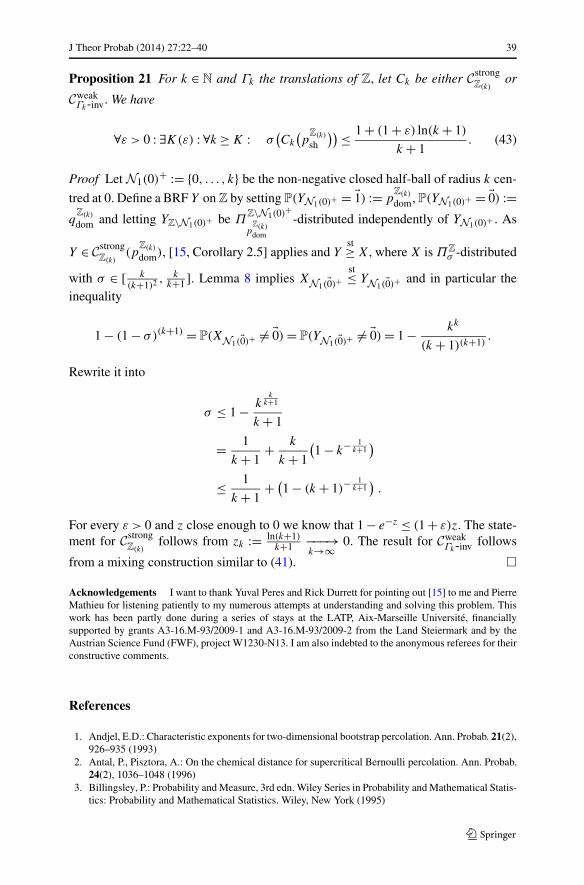
Proposition 21 For k ∈ N and Γk the translations of Z, let Ck be either C strongZ(k)

or

C weakΓk-inv. We have

∀ε > 0 : ∃K(ε) : ∀k ≥ K : σ(Ck

(p

Z(k)

sh

)) ≤ 1 + (1 + ε) ln(k + 1)

k + 1. (43)

Proof Let N1(0)+ := {0, . . . , k} be the non-negative closed half-ball of radius k cen-

tred at 0. Define a BRF Y on Z by setting P(YN1(0)+ = �1) := pZ(k)

dom, P(YN1(0)+ = �0) :=q

Z(k)

dom and letting YZ\N1(0)+ be ΠZ\N1(0)+

pZ(k)dom

-distributed independently of YN1(0)+ . As

Y ∈ C strongZ(k)

(pZ(k)

dom), [15, Corollary 2.5] applies and Yst≥ X, where X is ΠZ

σ -distributed

with σ ∈ [ k

(k+1)2 , kk+1 ]. Lemma 8 implies XN1(�0)+

st≤ YN1(�0)+ and in particular theinequality

1 − (1 − σ)(k+1) = P(XN1(�0)+ �= �0) = P(YN1(�0)+ �= �0) = 1 − kk

(k + 1)(k+1).

Rewrite it into

σ ≤ 1 − kk

k+1

k + 1

= 1

k + 1+ k

k + 1

(1 − k− 1

k+1)

≤ 1

k + 1+ (

1 − (k + 1)−1

k+1).

For every ε > 0 and z close enough to 0 we know that 1 − e−z ≤ (1 + ε)z. The state-ment for C strong

Z(k)follows from zk := ln(k+1)

k+1 −−−→k→∞ 0. The result for C weak

Γk-inv follows

from a mixing construction similar to (41). �

Acknowledgements I want to thank Yuval Peres and Rick Durrett for pointing out [15] to me and PierreMathieu for listening patiently to my numerous attempts at understanding and solving this problem. Thiswork has been partly done during a series of stays at the LATP, Aix-Marseille Université, financiallysupported by grants A3-16.M-93/2009-1 and A3-16.M-93/2009-2 from the Land Steiermark and by theAustrian Science Fund (FWF), project W1230-N13. I am also indebted to the anonymous referees for theirconstructive comments.

References

1. Andjel, E.D.: Characteristic exponents for two-dimensional bootstrap percolation. Ann. Probab. 21(2),926–935 (1993)

2. Antal, P., Pisztora, A.: On the chemical distance for supercritical Bernoulli percolation. Ann. Probab.24(2), 1036–1048 (1996)

3. Billingsley, P.: Probability and Measure, 3rd edn. Wiley Series in Probability and Mathematical Statis-tics: Probability and Mathematical Statistics. Wiley, New York (1995)

40 J Theor Probab (2014) 27:22–40

4. Bissacot, R., Fernández, R., Procacci, A.: On the convergence of cluster expansions for polymer gases.J. Stat. Phys. 139(4), 598–617 (2010)

5. Bissacot, R., Fernández, R., Procacci, A., Scoppola, B.: An improvement of the Lovász Local Lemmavia cluster expansion. Comb. Probab. Comput. (2011). doi:10.1017/S0963548311000253

6. Bollobás, B., Riordan, O.: Percolation. Cambridge University Press, Cambridge (2006)7. Dobrushin, R.L.: Perturbation methods of the theory of Gibbsian fields. In: Lectures on Probability

Theory and Statistics, Saint-Flour, 1994. Lecture Notes in Math., vol. 1648, pp. 1–66. Springer, Berlin(1996)

8. Erdos, P., Lovász, L.: Problems and results on 3-chromatic hypergraphs and some related questions.In: Infinite and Finite Sets (Colloq., Keszthely, 1973; dedicated to P. Erdos on his 60th birthday),vol. II. Colloquia Mathematica Societatis János Bolyai, vol. 10, pp. 609–627. North-Holland, Ams-terdam (1975)

9. Fernández, R., Procacci, A.: Cluster expansion for abstract polymer models. New bounds from an oldapproach. Commun. Math. Phys. 274(1), 123–140 (2007)

10. Fisher, D.C., Solow, A.E.: Dependence polynomials. Discrete Math. 82(3), 251–258 (1990)11. Grimmett, G.: Percolation, 2nd edn. Grundlehren der Mathematischen Wissenschaften [Fundamental

Principles of Mathematical Sciences], vol. 321. Springer, Berlin (1999)12. Gruber, C., Kunz, H.: General properties of polymer systems. Commun. Math. Phys. 22, 133–161

(1971)13. Hoede, C., Li, X.L.: Clique polynomials and independent set polynomials of graphs. Discrete Math.

125(1–3), 219–228 (1994). 13th British Combinatorial Conference (Guildford, 1991)14. Liggett, T.M.: Interacting Particle Systems. Classics in Mathematics. Springer, Berlin (2005). Reprint

of the 1985 original15. Liggett, T.M., Schonmann, R.H., Stacey, A.M.: Domination by product measures. Ann. Probab. 25(1),

71–95 (1997)16. Mathieu, P., Temmel, C.: K-independent percolation on trees. Stoch. Process. Appl. (2012). doi:

10.1016/j.spa.2011.10.01417. Russo, L.: An approximate zero–one law. Z. Wahrscheinlichkeitstheor. Verw. Geb. 61(1), 129–139

(1982)18. Scott, A.D., Sokal, A.D.: The repulsive lattice gas, the independent-set polynomial, and the Lovász

local lemma. J. Stat. Phys. 118(5–6), 1151–1261 (2005)19. Shearer, J.B.: On a problem of Spencer. Combinatorica 5(3), 241–245 (1985)20. Strassen, V.: The existence of probability measures with given marginals. Ann. Math. Stat. 36, 423–

439 (1965)