Embed Size (px)
Citation preview

© 2010 ANSYS, Inc. All rights reserved. 1 ANSYS, Inc. Proprietary© 2010 ANSYS, Inc. All rights reserved. 1 ANSYS, Inc. Proprietary
Shape optimisation
using breakthrough
technologies
Compiled by
Mike Slack
Ansys Technical Services

© 2010 ANSYS, Inc. All rights reserved. 2 ANSYS, Inc. Proprietary
Introduction
Shape optimisation
technologies
( Automated Invention? )

© 2010 ANSYS, Inc. All rights reserved. 3 ANSYS, Inc. Proprietary
Fast and Reliable Design
• Objective:
– Introduce two New and Elegant CFD shape
optimisation methods.
– Do my best to describe how they work.
– Explain how these can reliably reduce your
simulation time to find a shape optimised
design.

© 2010 ANSYS, Inc. All rights reserved. 4 ANSYS, Inc. Proprietary
Optimizsation
• The process of adjusting control variables to find the
levels that achieve the best possible outcome.
• The challenge is to achieve optimisation efficiently
– CFD runs can be long and expensive, even IO can be
significant.
– So we will consider systematic methods to find an optimum
response with a few trials
• Consider the different choice of technology, approach
and algorithm?

© 2010 ANSYS, Inc. All rights reserved. 5 ANSYS, Inc. Proprietary
Fast and Reliable Design
• The tools that will be presented are all available in
the current release.
• The Mesh Morph Optimiser is our first full release of
this technology type.
• The adjoint concept has been 10 years in the
making and is a unique offering in commercial CFD.
At this point the functionality is still Beta.

© 2010 ANSYS, Inc. All rights reserved. 6 ANSYS, Inc. Proprietary
Agenda
1. Introduction
2. Morphing
3. Linear shape optimisation methods
4. Derivative based optimisation method
5. Summary

© 2010 ANSYS, Inc. All rights reserved. 7 ANSYS, Inc. Proprietary
Morphing

© 2010 ANSYS, Inc. All rights reserved. 8 ANSYS, Inc. Proprietary
Mesh Morphing
• Applies a geometric design change directly in the
solver?
• Uses a Bernstein polynomial-based morphing
scheme
– Freeform mesh deformation defined on a matrix of control
points leads to a smooth deformation
• User prescribes the scale and direction of
deformations to control points distributed evenly
through the rectilinear region.

© 2010 ANSYS, Inc. All rights reserved. 9 ANSYS, Inc. Proprietary
Morpher
• Usage is based on the system of control points that can
be moved freely in space
© 2010 ANSYS, Inc. All rights reserved. 10 ANSYS, Inc. Proprietary
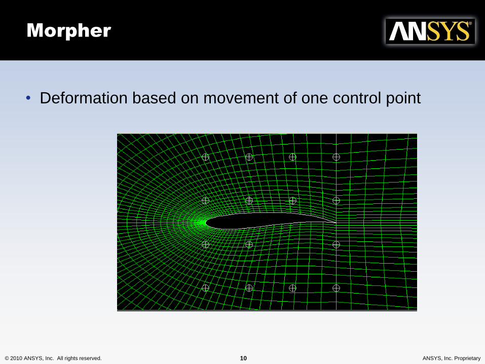
Morpher
• Deformation based on movement of one control point

© 2010 ANSYS, Inc. All rights reserved. 11 ANSYS, Inc. Proprietary
Morpher
• Deformation can be performed many times

© 2010 ANSYS, Inc. All rights reserved. 12 ANSYS, Inc. Proprietary
Morpher
• Deformation volume can have different numbers of
control points (example now uses five by two points)
© 2010 ANSYS, Inc. All rights reserved. 13 ANSYS, Inc. Proprietary
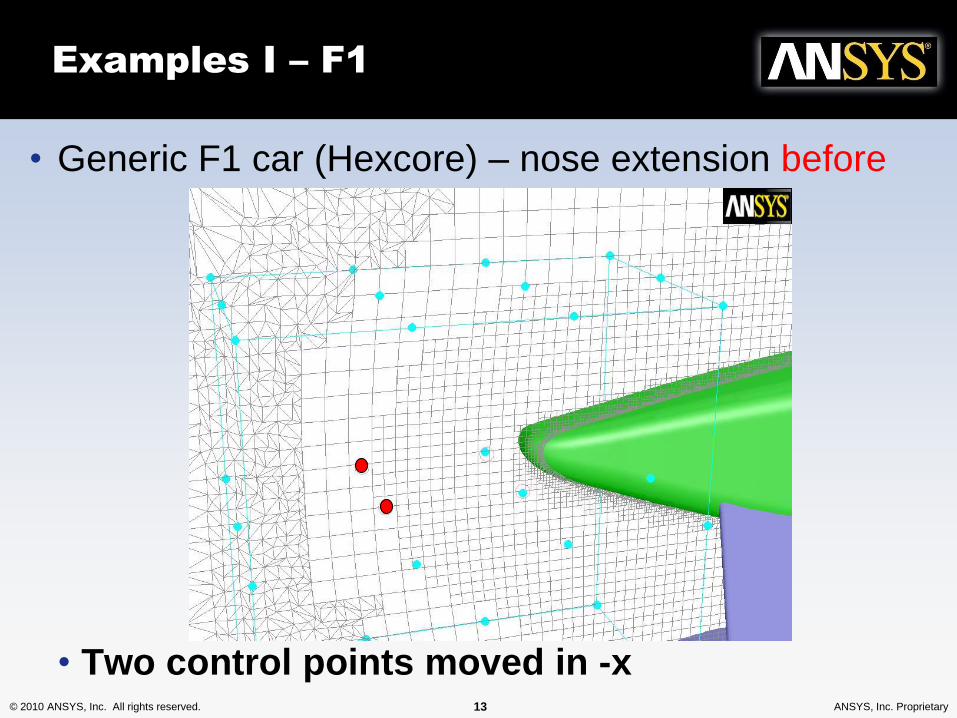
Examples I – F1
• Generic F1 car (Hexcore) – nose extension before
• Two control points moved in -x

© 2010 ANSYS, Inc. All rights reserved. 14 ANSYS, Inc. Proprietary
Examples I – F1
• Generic F1 car (Hexcore) – nose extension after
• Two control points moved in -x

© 2010 ANSYS, Inc. All rights reserved. 15 ANSYS, Inc. Proprietary
Mesh Morphing Workflow
• Stand Alone use of Morphing
1. Setup the CFD Problem
2. Perform the run
3. Identify improvements in the geometry
4. Use Morpher to modify the mesh in FLUENT itself
5. Run the solution on the modified geometry using
the previous result as an initial condition
6. For small variations in geometry the new solution
can be achieved very quickly
Note: With a little work the morph can be scripted or linked to
Workbench parameter using scheme variables

© 2010 ANSYS, Inc. All rights reserved. 16 ANSYS, Inc. Proprietary
Mesh Morpher Optimisation
(MMO)

© 2010 ANSYS, Inc. All rights reserved. 17 ANSYS, Inc. Proprietary
Mesh Morpher Optimiser (MMO)
• Workflow - Morpher coupled with optimiser
1. Setup the CFD problem
2. Invoke Mesh Morpher Tool
3. Define Objective Function
4. Define deformation region and assign deformation of control points through “Optimiser”
5. Perform solution to get the optimised design

© 2010 ANSYS, Inc. All rights reserved. 18 ANSYS, Inc. Proprietary
Objective Function
• Objective Function is a single scalar value that the chosen
optimizer method will drive towards a minimum.
• Typical Objective Functions– Lift & drag
– Mass flow-rate for inlets, outlets or internal plane
– Surface average pressures for walls/inlets/outlets
– Min-max absolute pressure/temperature etc.
• Objective Function is unrestricted and can be defined using,– User defined functions
– Scheme Function

© 2010 ANSYS, Inc. All rights reserved. 19 ANSYS, Inc. Proprietary
Example - Morpher with Shape
Optimizer
Application: L-shaped duct
Objective Function: Uniform flow at the outlet
Baseline Design Optimized Design

© 2010 ANSYS, Inc. All rights reserved. 20 ANSYS, Inc. Proprietary
Baseline Design Optimized Design
Example - Morpher with Shape
Optimizer
Application: Manifold
Objective Function: Equal flow rate through all the 18 nozzles

© 2010 ANSYS, Inc. All rights reserved. 21 ANSYS, Inc. Proprietary
Example – Simple Sedan
•Defining the deformation
•And shape variables

© 2010 ANSYS, Inc. All rights reserved. 22 ANSYS, Inc. Proprietary
Deformation Definition
1. Select individual control points and prescribe the relative
ranges of motion.
2. More than one direction and scale of motion can be
assigned using parameters
3. Choose an optimizer that will work to find the size of
deformation to apply to each parameter
Parameter 0

© 2010 ANSYS, Inc. All rights reserved. 23 ANSYS, Inc. Proprietary
What does Optimisation involve
• Lets consider the Simplex algorithm
– We need an objective
– Variables to be considered (geometric parameters)
• A k+1 geometric figure in a k-dimensional space is called a
simplex.
• k+1 is the number of trials to find the variables direction of
improvement.
Variable1 Variable1 Variable1
Va
ria
ble
2
Va
ria
ble
2
Dimensional Space

© 2010 ANSYS, Inc. All rights reserved. 24 ANSYS, Inc. Proprietary
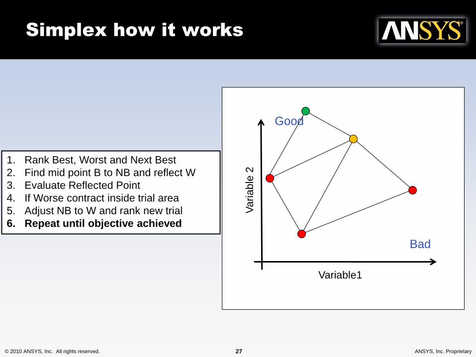
Simplex how it works
Variable1
Variable
2
Best
Next Best
Worst
Good
Bad
1. Rank Best, Worst and Next Best
2. Find mid point B to NB and reflect W
3. Evaluate Reflected Point
4. If Worse contract inside trial area
5. Adjust NB to W and rank new trial
6. Repeat until objective achieved

© 2010 ANSYS, Inc. All rights reserved. 25 ANSYS, Inc. Proprietary
Simplex how it works
Variable1
Variable
2
Good
Bad
1. Rank Best, Worst and Next Best
2. Find mid point B to NB and reflect W
3. Evaluate Reflected Point
4. If Worse contract inside trial area
5. Adjust NB to W and rank new trial
6. Repeat until objective achieved

© 2010 ANSYS, Inc. All rights reserved. 26 ANSYS, Inc. Proprietary
Simplex how it works
Variable1
Variable
2
Good
Bad
1. Rank Best, Worst and Next Best
2. Find mid point B to NB and reflect W
3. Evaluate Reflected Point
4. If Worse contract inside trial area
5. Adjust NB to W and rank new trial
6. Repeat until objective achieved
© 2010 ANSYS, Inc. All rights reserved. 27 ANSYS, Inc. Proprietary
Simplex how it works
Variable1
Variable
2
Good
Bad
1. Rank Best, Worst and Next Best
2. Find mid point B to NB and reflect W
3. Evaluate Reflected Point
4. If Worse contract inside trial area
5. Adjust NB to W and rank new trial
6. Repeat until objective achieved

© 2010 ANSYS, Inc. All rights reserved. 28 ANSYS, Inc. Proprietary
Simplex how it works
Variable1
Variable
2
Good
Bad
1. Rank Best, Worst and Next Best
2. Find mid point B to NB and reflect W
3. Evaluate Reflected Point
4. If Worse contract inside trial area
5. Adjust NB to W and rank new trial
6. Repeat until objective achieved

© 2010 ANSYS, Inc. All rights reserved. 29 ANSYS, Inc. Proprietary
Simplex how it works
Variable1
Variable
2
Good
Bad
1. Rank Best, Worst and Next Best
2. Find mid point B to NB and reflect W
3. Evaluate Reflected Point
4. If Worse contract inside trial area
5. Adjust NB to W and rank new trial
6. Repeat until objective achieved

© 2010 ANSYS, Inc. All rights reserved. 30 ANSYS, Inc. Proprietary
Simplex how it works
Variable1
Variable
2
Good
Bad
1. Rank Best, Worst and Next Best
2. Find mid point B to NB and reflect W
3. Evaluate Reflected Point
4. If Worse contract inside trial area
5. Adjust NB to W and rank new trial
6. Repeat until objective achieved

© 2010 ANSYS, Inc. All rights reserved. 31 ANSYS, Inc. Proprietary
Baseline Design Optimized Design
Application: Incompressible turbulent flow over a car
Objective Function: Minimise Drag
Example - Morpher with Shape
Optimizer

© 2010 ANSYS, Inc. All rights reserved. 32 ANSYS, Inc. Proprietary
Generic HVAC Duct
• HVAC duct section of an aircraft
with one main outlet and two side
outlets
• Objective:
• Minimize pressure drop in the
duct by optimizing the shape of
branch-2
Inlet
Velocity = 10m/s
main outlet
Pressure = 0 Pa
branch outlets
Pressure = 0 Pa
branch 1
branch 2
BaselineModified

© 2010 ANSYS, Inc. All rights reserved. 33 ANSYS, Inc. Proprietary
Adjoint method

© 2010 ANSYS, Inc. All rights reserved. 34 ANSYS, Inc. Proprietary
What does an adjoint solver do?
• An adjoint solver provides specific information about a
fluid system that is very difficult to gather otherwise.
• An adjoint solver can be used to compute the derivative
of an engineering quantity with respect to all of the inputs
for the system.
• For example
– Derivative of drag with respect to the shape of a vehicle.
– Derivative of total pressure drop with respect the shape of the
flow path.

© 2010 ANSYS, Inc. All rights reserved. 35 ANSYS, Inc. Proprietary
Key Ideas - Fundamentals
FLOW SOLVER
Inputs
• Boundary mesh
• Interior mesh
• Material properties
• Boundary condition 1
• Flow angle
• Inlet velocity
• …
• …
Outputs
• Field data
• Contour plots
• Vector plots
• xy-plots
• Scalar values
• Lift
• Drag
• Total pressure drop
High-level “system” view of a conventional flow solver
© 2010 ANSYS, Inc. All rights reserved. 36 ANSYS, Inc. Proprietary
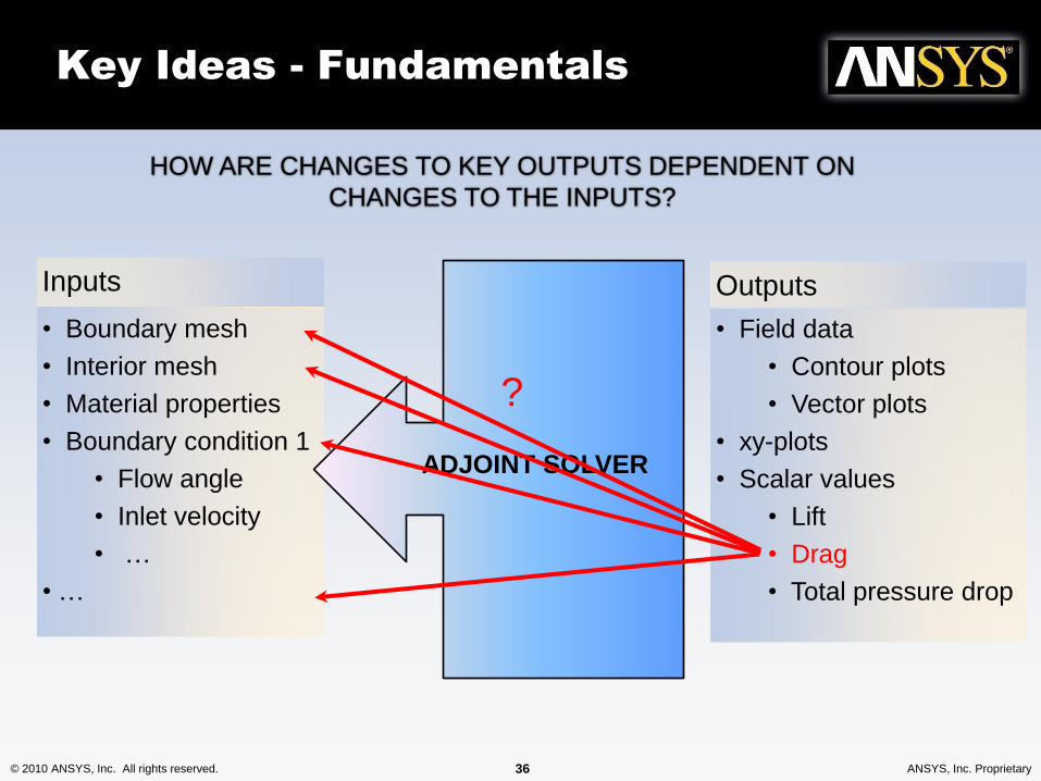
Key Ideas - Fundamentals
Inputs
• Boundary mesh
• Interior mesh
• Material properties
• Boundary condition 1
• Flow angle
• Inlet velocity
• …
• …
Outputs
• Field data
• Contour plots
• Vector plots
• xy-plots
• Scalar values
• Lift
• Drag
• Total pressure drop
HOW ARE CHANGES TO KEY OUTPUTS DEPENDENT ON
CHANGES TO THE INPUTS?
ADJOINT SOLVER
?
© 2010 ANSYS, Inc. All rights reserved. 37 ANSYS, Inc. Proprietary
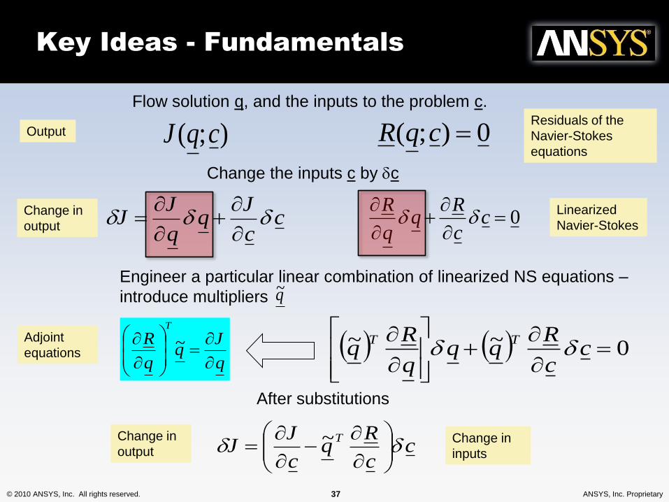
Key Ideas - Fundamentals
Flow solution q, and the inputs to the problem c.
);( cqJOutput 0);( cqRResiduals of the
Navier-Stokes
equations
0
c
c
Rq
q
R Linearized
Navier-Stokes
Change the inputs c by c
cc
Jq
q
JJ
Change in
output
Engineer a particular linear combination of linearized NS equations –
introduce multipliers
0~~
c
c
Rqq
q
Rq
TT
q~
q
Jq
q
RT
~Adjoint
equations
After substitutions
cc
Rq
c
JJ
T
~ Change in
inputs
Change in
output

© 2010 ANSYS, Inc. All rights reserved. 38 ANSYS, Inc. Proprietary
• Construct and solve an adjoint problem to get a helper
solution
• Solve using AMG
• Involves a familiar process
– Solution advancement controls – Courant number, under-
relaxation
– Residuals & iterations
– Roughly the same effort as a conventional flow solution
Key Ideas – Adjoint Equations
This innocent-looking
system of equations is at
the heart of the adjoint
solver.q
Jq
q
RT
~

© 2010 ANSYS, Inc. All rights reserved. 39 ANSYS, Inc. Proprietary
Key Ideas – Shape Sensitivity
Shape sensitivity: Sensitivity of the observed value with
respect to (boundary) grid node locations
mesh
nnxwDrag .)(
Shape sensitivity coefficients:
Vector field defined
on mesh nodes
Node displacement
Visualization of shape sensitivity
• Uses vector field visualization.
• Identifies regions of high and low
sensitivity.
Drag sensitivity for NACA0012

© 2010 ANSYS, Inc. All rights reserved. 40 ANSYS, Inc. Proprietary
Key Ideas – Mesh Moprhing
Actual change 3.1
DP = -213.8
Total improvement
of 8%
Constrained motion
• Some walls within the control volume may be constrained not
to move.

© 2010 ANSYS, Inc. All rights reserved. 41 ANSYS, Inc. Proprietary
Pressure drop reduction example

© 2010 ANSYS, Inc. All rights reserved. 42 ANSYS, Inc. Proprietary
Key Ideas – Mesh Adaptation
Solution-based mesh adaptation
• Regions in the flow domain where the
adjoint solution is large have a strong
effect of discretization errors in the
quantity of interest.
• Adapt in regions where the adjoint
solution is large
Adjoint solution
Drag sensitivity
Baseline Mesh
Adapted Mesh
Adapted Mesh
Detail

© 2010 ANSYS, Inc. All rights reserved. 43 ANSYS, Inc. Proprietary
Current Functionality
• ANSYS-Fluent flow solver has very broad scope
• Adjoint is configured to compute solutions based on some
assumptions
– Steady, incompressible, laminar flow.
– Steady, incompressible, turbulent flow with standard wall functions.
– First-order discretization in space.
– Frozen turbulence.
• The primary flow solution does NOT need to be run with these
restrictions
– Strong evidence that these assumptions do not undermine the utility of
the adjoint solution data for engineering purposes.
• Fully parallelized.
• Gradient algorithm for shape modification
– Mesh morphing using control points.
• Adjoint-based solution adaption
© 2010 ANSYS, Inc. All rights reserved. 44 ANSYS, Inc. Proprietary
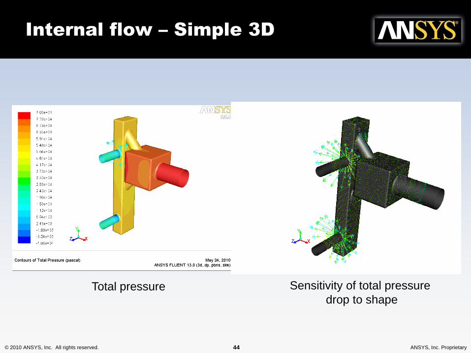
Internal flow – Simple 3D
Total pressure Sensitivity of total pressure
drop to shape

© 2010 ANSYS, Inc. All rights reserved. 45 ANSYS, Inc. Proprietary
Internal flow – Simple 3D
Total pressure drop = -23765 Pa
Predicted change = 2858 Pa
Actual change = 2390 Pa

© 2010 ANSYS, Inc. All rights reserved. 46 ANSYS, Inc. Proprietary
180° Elbow optimization
0
10
20
30
40
50
60
70
80
90
100
0 10 20 30
Dp
tot[P
a]
Run [-]
Thanks to Hauke Reese
ANSYS Germany

© 2010 ANSYS, Inc. All rights reserved. 47 ANSYS, Inc. Proprietary
180 Elbow: Optimization Loop
Base design End design
© 2010 ANSYS, Inc. All rights reserved. 48 ANSYS, Inc. Proprietary
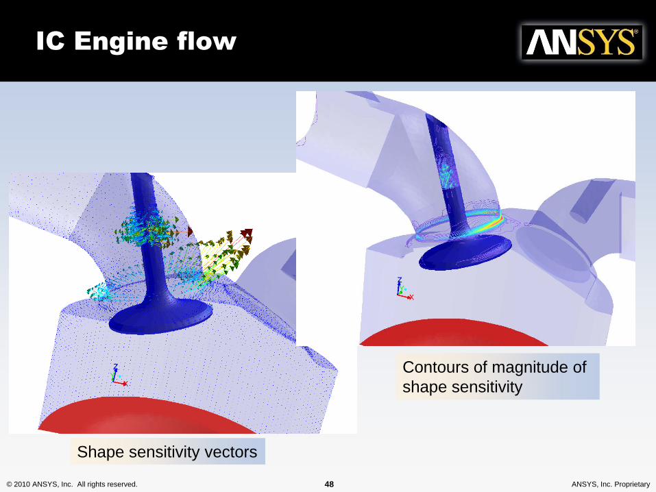
IC Engine flow
Adjoint Residuals
Shape sensitivity vectors
Contours of magnitude of
shape sensitivity
© 2010 ANSYS, Inc. All rights reserved. 49 ANSYS, Inc. Proprietary
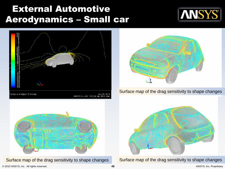
External Automotive
Aerodynamics – Small car
Surface map of the drag sensitivity to shape changes
Surface map of the drag sensitivity to shape changesSurface map of the drag sensitivity to shape changes
© 2010 ANSYS, Inc. All rights reserved. 50 ANSYS, Inc. Proprietary
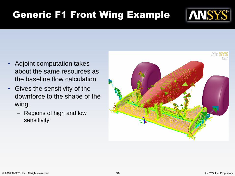
• Adjoint computation takes
about the same resources as
the baseline flow calculation
• Gives the sensitivity of the
downforce to the shape of the
wing.
– Regions of high and low
sensitivity
Generic F1 Front Wing Example

© 2010 ANSYS, Inc. All rights reserved. 51 ANSYS, Inc. Proprietary
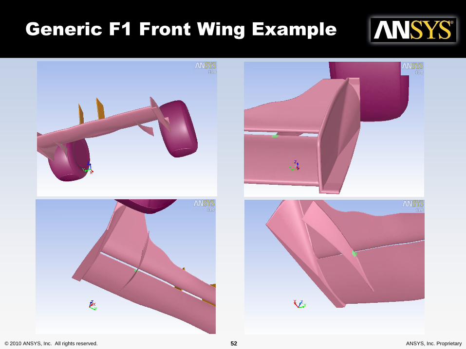
Adjoint solution:
• Quantifies the effect of specific
changes to shape upon downforce
• Suggests an optimal modification to
the shape to enhance downforce
Baseline downforce = 905.4N
Predicted improvement = 41.6N
Actual improvement = 39.1N
Generic F1 Front Wing Example
© 2010 ANSYS, Inc. All rights reserved. 52 ANSYS, Inc. Proprietary
Generic F1 Front Wing Example

© 2010 ANSYS, Inc. All rights reserved. 53 ANSYS, Inc. Proprietary
Summary

© 2010 ANSYS, Inc. All rights reserved. 54 ANSYS, Inc. Proprietary
Summary
• Two new approaches to consider
– The morpher and optimisation provide efficient tool to make and
compare geometric adjustments.
– Consider using the adjoint to guide the morpher.
– The Adjoint alone is also very useful to identify key sensitivities.
• These are new technologies which will continue to be
enhanced.
• We encourage you to consider these techniques and will
be happy to assist you.