Shape Fitting on Point Sets with ProbabilityDistributions

Maarten Loffler

Jeff Phillips

Technical Report UU-CS-2009-013June 2009

Department of Information and Computing Sciences

Utrecht University, Utrecht, The Netherlandswww.cs.uu.nl

ISSN: 0924-3275

Department of Information and Computing SciencesUtrecht UniversityP.O. Box 80.0893508 TB UtrechtThe Netherlands

Shape Fitting on Point Sets with Probability Distributions

Maarten LofflerUtrecht Universityloffler@cs.uu.nl

Jeff PhillipsDuke University

jeffp@cs.duke.edu

June 25, 2009

Abstract

We consider problems on data sets where each data point has uncertainty described by an individualprobability distribution. We develop several frameworks and algorithms for calculating statistics on theseuncertain data sets. Our examples focus on geometric shape fitting problems. We prove approximationguarantees for the algorithms with respect to the full probability distributions. We then empiricallydemonstrate that our algorithms are simple and practical, solving for a constant hidden by asymptoticanalysis so that a user can reliably trade speed and size for accuracy.

1 Introduction

This paper deals with data sets where each “data point” is actually a distribution of where a data point maybe. We focus on geometric problems on this data, however, many of the ideas, data structures, and algorithmsextend to non-geometric problems. Since the input data we consider has uncertainty, given by probabilitydistributions, we argue that computing exact answers may not be worth the effort. Furthermore, manyproblems we consider may not have compact closed form solutions. As a result, we produce approximateanswers.

Sensed Data

In gathering data there is a trade-off between quantity and accuracy. The drop in the price of hard drivesand other storage costs has shifted this balance towards gathering enormous quantities of data, yet withnoticeable and sometimes intentional imprecision. However, often as a benefit from the large data sets,models are developed to describe the pattern of the data error.

Let us take as an example Light Detection and Ranging (LIDAR) data gathered for Geographic Infor-mation Systems (GIS) [27], specifically height values at millions of locations on a terrain. Each data point(x, y, z) has an x-value (longitude), a y-value (latitude), and a z-value (height). This data set is gathered bya small plane flying over a terrain with a laser aimed at the ground measuring the distance from the plane tothe ground. Error can occur due to inaccurate estimation of the plane’s altitude and position or artifacts onthe ground distorting the laser’s distance reading. But these errors are well-studied and can be modeled byreplacing each data point with a probability distribution of its actual position. Greatly simplifying, we couldrepresent each data point as a 3-variate normal distribution centered at its recorded value.

Similarly, large data sets are gathered and maintained for many other applications. In robotic mapping [39,16] error models are provided for data points gathered by laser range finders and other sources. In datamining [1, 5] original data (such as published medical data) are often perturbed by a known model topreserve anonymity. In spatial databases [20, 37, 13] large data sets may be summarized as probabilitydistributions to store them more compactly. Sensor networks [15] stream in large data sets collected bycheap and thus inaccurate sensors. In protein structure determination [35] every atom’s position is imprecisedue to inaccuracies in reconstruction techniques and the inherent flexibility in the protein. In summary, thereare many large data sets with modeled errors and dynamic updates.

However, much raw data is not immediately given as a set of probability distributions, rather as a set ofpoints, each essentially drawn from a probability distribution itself. Approximate algorithms may treat thisdata as exact, construct an approximate answer, and then postulate that since the raw data is not exact andhas inaccuracies, the approximation errors made by the algorithm may be similar to the inaccuracies of theimprecise input data. This is a very dangerous postulation, as demonstrated by the following example.

Example. Consider a robot trying to determine the boundary of a convex room. Its strategy is to use alaser range finder to get data points on objects in the room (hopefully boundary walls), and then take theconvex hull of these points.

However, large errors may occur if the room has windows; a few laser scans may not bounce off thewindow, and thus return data points (say, 100 meters) outside the room. Standard techniques (e.g., α-kernels) would include those points in the convex hull, but may allow some approximation (say, up to 10meters). Hence, the outlier data points could still dramatically warp the shape of the room, outside the errortolerance.

However, an error model on these outlier data points, through regression to the mean, would assign someprobability to them being approximately correct and some probability to them actually being inside (ormuch closer to) the true room. An algorithm which took this error model into account would assign some

1

probability of a shape near the true room shape and some probability to the oblong room that extends outthrough the window.

It is clear from this example, that an algorithm can only provide answers as good as the raw data andthe models for error on that data. This paper is not about how to construct error models, but how to takeerror models into account. While many existing algorithms produce approximations with respect only to theraw input data, algorithms in this paper approximate with respect to the raw input data and the error modelsassociated with them.

Other geometric error models. The input for a typical computational geometry problem is a set P of npoints in R2, or more generally Rd. Traditionally, such a set of points is assumed to be known exactly, andindeed, in the 1980s and 1990s such an assumption was often justified because much of the input data washand-constructed for computer graphics or simulations. However, in many modern applications the input issensed from the real world, and such data is inherently imprecise. Therefore, there is a growing need formethods that are able to deal with imprecision.

An early model to quantify imprecision in geometric data, motivated by finite precision of coordinates,is ε-geometry, introduced by Guibas et al. [18]. In this model, the input is given by a traditional point setP , where the imprecision is modeled by a single extra parameter ε. The true point set is not known, but itis certain that for each point in P there is a point in the disk of radius ε around it. This model has provenfruitful and is still often used due to its simplicity. To name a few examples, Guibas et al. [19] define stronglyconvex polygons: polygons that are guaranteed to stay convex, even when the vertices are perturbed by ε.Bandyopadhyay and Snoeyink [7] compute the set of all potential simplices in R2 and R3 that could belongto the Delaunay triangulation. Held and Mitchell [23] and Loffler and Snoeyink [28] study the problem ofpreprocessing a set of imprecise points under this model, so that when the true points are specified latersome computation can be done faster.

A more involved model for imprecision can be obtained by not specifying a single ε for all the points,but allowing a different radius for each point, or even other shapes of imprecision regions. This allows formodeling imprecision that comes from different sources, independent imprecision in different dimensionsof the input, etc. This extra freedom in modeling comes at the price of more involved algorithmic solutions,but still many results are available. Nagai and Tokura [32] compute the union and intersection of all possibleconvex hulls to obtain bounds on any possible solution, as does Ostrovsky-Berman and Joskowicz [33]in a setting allowing some dependence between points. Van Kreveld and Loffler [40] study the problemof computing the smallest and largest possible values of several geometric extent measures, such as thediameter or the radius of the smallest enclosing ball, where the points are restricted to lie in given regions inthe plane. Kruger [25] extends some of these results to higher dimensions.

These models, in general, give worst case bounds on error, for instance upper and lower bounds onthe radius of the minimum enclosing ball. When the error is derived entirely from precision errors, thisinformation can be quite useful (as much of theoretical computer science is based on worst case bounds).However, when data is sensed, the maximum error range used as input are often manufactured by truncatinga probability distribution, so the probability that a point is outside that range is below some threshold. Sincethe above models usually produce algorithms and answers very dependent on boundary cases, these artificial(and sometimes arbitrary) thresholds play large roles in the answers. Furthermore, the true location of thedata points are often not near the boundary of the error range, but near the center. Hence, it makes moresense to use the original probability distributions, and then if needed, we can apply a threshold based onprobability to the final solution. This ensures that the truncation errors have not accumulated.

This paper studies the computation of extent measures on uncertain point sets governed by probabilitydistributions. Unsurprisingly, directly using the probability distribution error model creates harder algorith-mic problems, and many questions may be impossible to answer exactly under this model. But since the

2

data is imprecise to begin with, it is also reasonable to construct approximate answers. Our algorithms haveapproximation guarantees with respect to the original distributions, not an approximation of them. Thismodel of uncertain data has been studied in the database community but for different types of problems (e.g.indexing[38, 24] and nearest neighbor[12]) and approximation guarantees. We focus on computing statisticson uncertain point sets, specifically shape fitting problems in a way that allows the uncertain data problemto be reduced to well-studied techniques on discrete point sets.

1.1 Problem Statement

Let µp : Rd → R+ describe the probability distribution of a point p where the integral∫q∈Rd µp(q) dq = 1.

Let µP : Rd × Rd × . . . × Rd → R+ describe the distribution of a point set P by the joint probabilityover each p ∈ P . For brevity we write the space Rd × . . . × Rd as Rdn. For this paper we will assumeµP (q1, q2, . . . , qn) =

∏ni=1 µpi(qi), so the distribution for each point is independent, although this restric-

tion can be easily circumvented.Given a distribution µP we ask a variety of shape fitting questions about the uncertain point set. For

instance, what is the radius of the smallest enclosing ball or what is the smallest axis-aligned bounding boxof an uncertain point set. In the presence of imprecision, the answer to such a question is not a single valueor structure, but also a distribution of answers. The focus of this paper is not just how to answer such shapefitting questions about these distributions, but how to concisely represent them. As a result, we introducetwo types of approximate distributions as answers, and a technique to construct coresets for these answers.

ε-Quantizations. Let f : Rdn → Rk be a function on a fixed point set. Examples include the radius ofthe minimum enclosing ball where k = 1 and the width of the minimum enclosing axis-aligned rectanglealong the x-axis and y-axis where k = 2. Define the “dominates” binary operator � so that (p1, . . . , pk) �(v1, . . . , vk) is true if for every coordinate pi ≤ vi. Let Xf (v) = {Q ∈ Rdn | f(Q) � v}. For a query valuev define,

FµP (v) =∫

Q∈Xf (v)µP (Q) dQ.

Then FµP is the cumulative density function of the distribution of possible values that f can take1. Ideally,we would return the function FµP so we could quickly answer any query exactly, however, it is not clear howto calculate FµP (v) exactly for even a single query value v. Rather, we introduce a data structure, which

1For a function f and a distribution of point sets µP , we will always represent the cumulative density function of f over µP byFµP .

(a) (b)

(d) (c)

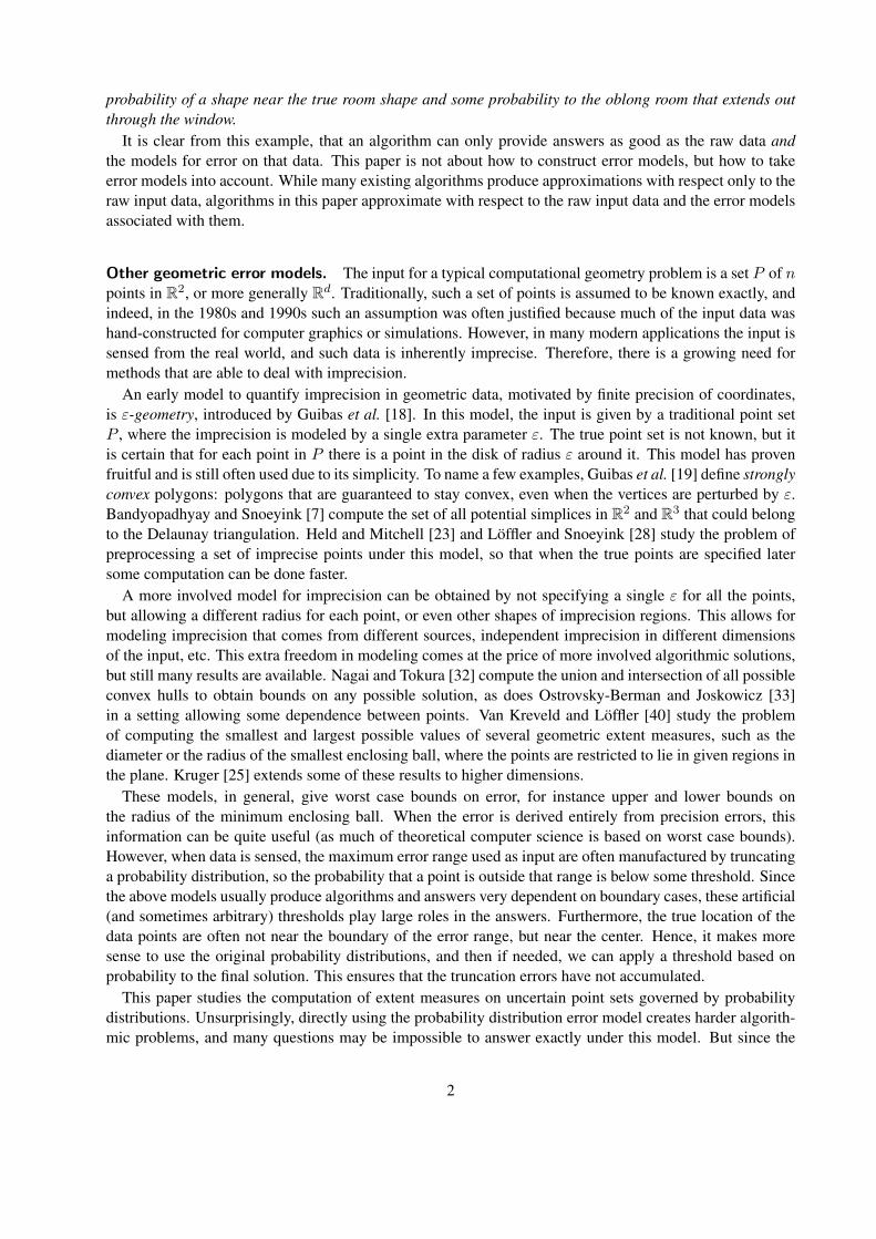
Figure 1: (a) The true form of a monotonically increasing function from R → R. (b) The ε-quantization Ras a point set in R. (c) The inferred curve hR in R2. (d) Overlay of the two images.

3

we call an ε-quantization, to answer any such query approximately and efficiently, illustrated in Figure 1 fork = 1. An ε-quantization is a point set R ⊂ Rk which induces a function hR where hR(v) describes thefraction of points in R that v dominates. Let Rv = {r ∈ R | r � v}. Then hR(v) = |Rv|/|R|. For anisotonic (monotonically increasing in each coordinate) function FµP and any value v, an ε-quantization, R,guarantees that

|hR(v)− FµP (v)| ≤ ε.

More generally (and, for brevity, usually only when k > 1), we say R is a k-variate ε-quantization. Anexample of a 2-variate ε-quantization is shown in Figure 2. The space required to store the data structure forR is dependent only on ε and k, not on |P | or µP .

(a) (b) (c) (d)

Figure 2: (a) The true form of a 2-variate function. (b) The ε-quantization R as a point set in R2. (c) Theinferred surface hR in R3. (d) Overlay of the two images.

(ε, δ, α)-Kernels. Rather than compute a new data structure for each measure we are interested in, wecan also compute a single data structure (a coreset) that allows us to answer many types of questions. Foran isotonic function FµP : R+ → [0, 1], an (ε, α)-quantization data structure M describes a function hM :R+ → [0, 1] so for any x ∈ R+, there is an x′ ∈ R+ such that (1) |x−x′| ≤ αx and (2) |hM (x)−FµP (x′)| ≤ε. An (ε, δ, α)-kernel is a data structure that can produce an (ε, α)-quantization, with probability at least1−δ, for FµP where f measures the width in any direction and whose size depends only on ε, α, and δ. Thenotion of (ε, α)-quantizations is generalized to a k-variate version, as are (ε, δ, α)-kernels, in Section 2.2.

Shape inclusion probabilities. A summarizing shape of a point set P ⊂ Rd is a Lebesgue-measureablesubset of Rd that is determined by P . Examples include the smallest enclosing ball, the minimum-volumeaxis-aligned bounding box, or the convex hull. We consider some class of shapes S and the summarizingshape S(P ) ∈ S is the shape from S that is optimized in some aspect with respect to P . For a family ofsummarizing shapes S we can study the shape inclusion probability function sµP : Rd → [0, 1] (or sipfunction), where sµP (q) describes the probability that a query point q ∈ Rd is included in the summarizingshape2. There does not seem to be a closed form for many of these functions. Rather we calculate an ε-sipfunction s : Rd → [0, 1] such that ∀q∈Rd |sµP (q)− s(q)| ≤ ε. The space required to store an ε-sip functiondepends only on ε and the complexity of the summarizing shape.

1.2 Contributions

We describe simple and practical randomized algorithms for the computation of ε-quantizations, (ε, δ, α)-kernels, and ε-sip functions. Let Tf (n) be the time it takes to calculate a summarizing shape of a set of n

2For technical reasons, if there are (degenerately) multiple optimal summarizing shapes, we say each is equally likely to be thesummarizing shape of the point set.

4

points Q ⊂ Rd, which generates a statistic f(Q) (e.g., radius of smallest enclosing ball). We can calculatean ε-quantization of FµP , with probability at least 1 − δ, in time O(Tf (n)(1/ε2) log(1/δ)). For univariateε-quantizations the size is O(1/ε), and for k-variate ε-quantizations the size is O(k2(1/ε) log2k(1/ε)). Wecan calculate an (ε, δ, α)-kernel of size O((1/α(d−1)/2)·(1/ε2) log(1/δ)) in O((n+(1/αd−3/2))(1/ε2) log(1/δ))time. With probability at least 1− δ, we can calculate an ε-sip function of size O((1/ε2) log(1/δ)) in timeO(Tf (n)(1/ε2) log(1/δ)).

All of these randomized algorithms are simple and practical, as demonstrated by a series of experimentalresults. In particular, we show that the constant hidden by the big-O notation is in practice at most 0.5 forall algorithms.

This paper describes results for shape fitting problems for distributions of point sets in Rd, in particular, wewill use the smallest enclosing ball and the axis-aligned bounding box as running examples in the algorithmdescriptions. The concept of ε-quantizations extends to many other problems with uncertain data. In fact,variations of our randomized algorithm will work for a more general array of problems.

1.3 Preliminaries: ε-Samples and α-Kernels

ε-Samples. For a set P let A be a set of subsets of P . In our context usually P will be a point set and thesubsets in A could be induced by containment in a shape from some family of geometric shapes. For someexamples of A, let Br describe all subsets of P determined by containment in some ball of radius r; let Rd

describe all subsets of P defined by containment in some d-dimensional axis-aligned box; let H describe allsubsets of P defined by containment in some halfspace. We use A generically to represent one such familyof ranges.

The pair (P,A) is called a range space. We say that Q ⊂ P is an ε-sample of (P,A) if

∀R∈A

∣∣∣∣φ(R ∩Q)φ(Q)

− φ(R ∩ P )φ(P )

∣∣∣∣ ≤ ε,

where | · | takes the absolute value and φ(·) returns the measure of a point set. In the discrete case φ(Q)returns the cardinality of Q. We say A shatters a set S if every subset of S is equal to R ∩ S for someR ∈ A. The cardinality of the largest discrete set S ⊆ P that A can shatter is known as the VC-dimensionof (P,A).

When (P,A) has constant VC-dimension ν, we can create an ε-sample Q of (P,A), with probability1 − δ, by uniformly sampling O((1/ε2)(ν + log(1/δ))) points from P [41, 26]. There exist deterministictechniques to create ε-samples [29, 11] of size O(ν(1/ε2) log(1/ε)) in time O(ν3νn((1/ε2) log(ν/ε))ν).There exist ε-samples of smaller sizes [31], but direct, efficient constructions are not known. When P isa point set in Rd and the family of ranges Qk is determined by inclusion of convex shapes whose sideshave one of k predefined normal directions, such as the set of axis-aligned boxes, then an ε-sample for(P,Qk) of size O((k/ε) log2k(1/ε)) can be constructed in O((n/ε3) log6k(1/ε)) time [34]. If (P,A) hasVC-dimension ν, this also implies that (P,A) contains at most |P |ν sets.

For a range space (P,A) the dual range space is defined (A, P ∗) where P ∗ is all subsetsAp ⊆ A definedfor an element p ∈ P such that Ap = {A ∈ A | p ∈ A}. If (P,A) has VC-dimension ν, then (A, P ∗)has VC-dimension ≤ 2ν+1. Thus, if the VC-dimension of (A, P ∗) is constant, then the VC-dimension of(P,A) is also constant [30]. Hence, the standard ε-sample theorems apply to dual range spaces as well.

When we have a distribution µ : Rd → R+, such that∫x∈R µ(x) dx = 1, we can think of this as the set

P of all points in Rd, where the weight w of a point p ∈ Rd is µ(p). Hence, if a point is randomly selectedfrom P proportional to its weight w, then it is equivalent to selecting a point at random from the distributionµ. To simplify notation, we write (µ,A) as a range space where the ground set is this set P = Rd weightedby the distribution µ.

5

Let g : R → R+ be a function where∫∞x=−∞ g(x) dx = 1. We can create an ε-sample Qg of (g, I+),

where I+ describes the set of all one-sided intervals of the form (−∞, t), so that

maxt

∣∣∣∣∣∣∫ t

x=−∞g(x) dx− 1

|Qg|∑q∈Qg

1(q < t)

∣∣∣∣∣∣ ≤ ε.

We can construct Qg of size O(1ε ) by choosing a set of points in Qg so that the integral between two

consecutive points is always ε. But we do not need to be so precise. Consider the set of d2/εe points{q′1, q′2, . . . , q′d2/εe} such that

∫ q′i

x=−∞ = iε/2. Any set of d2/εe points Qg = {q1, q2, . . . , qd2/εe} such thatq′i ≤ qi ≤ q′i+1 is an ε-sample.

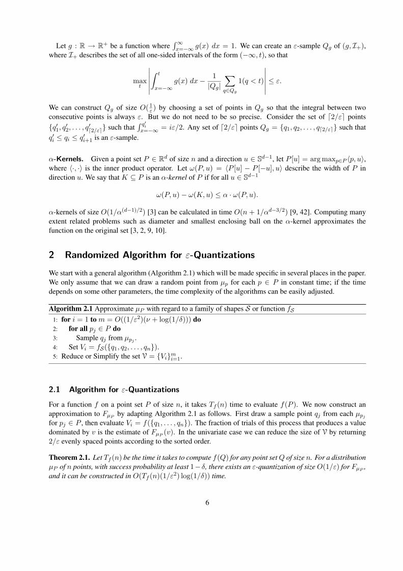
α-Kernels. Given a point set P ∈ Rd of size n and a direction u ∈ Sd−1, let P [u] = arg maxp∈P 〈p, u〉,where 〈·, ·〉 is the inner product operator. Let ω(P, u) = 〈P [u] − P [−u], u〉 describe the width of P indirection u. We say that K ⊆ P is an α-kernel of P if for all u ∈ Sd−1

ω(P, u)− ω(K, u) ≤ α · ω(P, u).

α-kernels of size O(1/α(d−1)/2) [3] can be calculated in time O(n + 1/αd−3/2) [9, 42]. Computing manyextent related problems such as diameter and smallest enclosing ball on the α-kernel approximates thefunction on the original set [3, 2, 9, 10].

2 Randomized Algorithm for ε-Quantizations

We start with a general algorithm (Algorithm 2.1) which will be made specific in several places in the paper.We only assume that we can draw a random point from µp for each p ∈ P in constant time; if the timedepends on some other parameters, the time complexity of the algorithms can be easily adjusted.

Algorithm 2.1 Approximate µP with regard to a family of shapes S or function fS

1: for i = 1 to m = O((1/ε2)(ν + log(1/δ))) do2: for all pj ∈ P do3: Sample qj from µpj .4: Set Vi = fS({q1, q2, . . . , qn}).5: Reduce or Simplify the set V = {Vi}m

i=1.

2.1 Algorithm for ε-Quantizations

For a function f on a point set P of size n, it takes Tf (n) time to evaluate f(P ). We now construct anapproximation to FµP by adapting Algorithm 2.1 as follows. First draw a sample point qj from each µpj

for pj ∈ P , then evaluate Vi = f({q1, . . . , qn}). The fraction of trials of this process that produces a valuedominated by v is the estimate of FµP (v). In the univariate case we can reduce the size of V by returning2/ε evenly spaced points according to the sorted order.

Theorem 2.1. Let Tf (n) be the time it takes to compute f(Q) for any point set Q of size n. For a distributionµP of n points, with success probability at least 1−δ, there exists an ε-quantization of size O(1/ε) for FµP ,and it can be constructed in O(Tf (n)(1/ε2) log(1/δ)) time.

6

Proof. Because FµP : R → [0, 1] is an isotonic function, there exists another function g : R → R+ suchthat FµP (t) =

∫ tx=−∞ g(x) dx where

∫x∈R g(x) dx = 1. Thus g is a probability distribution of the values

of f given inputs drawn from µP . This implies that an ε-sample of (g, I+) is an ε-quantization of FµP , sinceboth estimate within ε the fraction of points in any range of the form (−∞, x).

By drawing a random sample qi from each µpi for pi ∈ P , we are drawing a random point set Q from µP .Thus f(Q) is a random sample from g. Hence, using the standard randomized construction for ε-samples,O((1/ε2) log(1/δ)) such samples will generate an (ε/2)-sample for g, and hence an (ε/2)-quantization forFµP , with probability at least 1− δ.

Since in an (ε/2)-quantization R every value hR(v) is different from FµP (v) by at most ε/2, then wecan take an (ε/2)-quantization of the function described by hR(·) and still have an ε-quantization of FµP .Thus, we can reduce this to an ε-quantization of size O(1/ε) by taking a subset of 2/ε points spaced evenlyaccording to their sorted order.

We can construct k-variate ε-quantizations using the same basic procedure as in Algorithm 2.1. Theoutput Vi of fS is k-variate and thus results in a k-dimensional point.

Theorem 2.2. Let Tf (n) be the time it takes to compute f(Q) for any point set Q of size n. Given a distri-bution µP of n points, with success probability at least 1 − δ, we can construct a k-variate ε-quantizationfor FµP of size O((k/ε2)(k + log(1/δ))) and in time O(Tf (n)(1/ε2)(k + log(1/δ))).

Proof. Let R+ describe the family of ranges where a range Ap = {q ∈ Rk | q � p}. In the k-variate casethere exists a function g : Rk → R+ such that FµP (v) =

∫x�v g(x) dx where

∫x∈Rk g(x) dx = 1. Thus

g describes the probability distribution of the values of f , given inputs drawn randomly from µP . Hencea random point set Q from µP , evaluated as f(Q), is still a random sample from the k-variate distributiondescribed by g. Thus, with probability at least 1 − δ, a set of O((1/ε2)(k + log(1/δ))) such samples isan ε-sample of (g,R+), which has VC-dimension k, and the samples are also a k-variate ε-quantization ofFµP .

We can then reduce the size of the ε-quantization R to O((k2/ε) log2k(1/ε)) in O(|R|(k/ε3) log6k(1/ε))time [34] or to O((k2/ε2) log(1/ε)) in O(|R|(k3k/ε2k) · logk(k/ε)) time [11], since the VC-dimension isk and each data point requires O(k) storage. However, we do not investigate the empirical performance ofthese deterministic algorithms in this paper. See [6] for an empirical study of alternatives to [11].

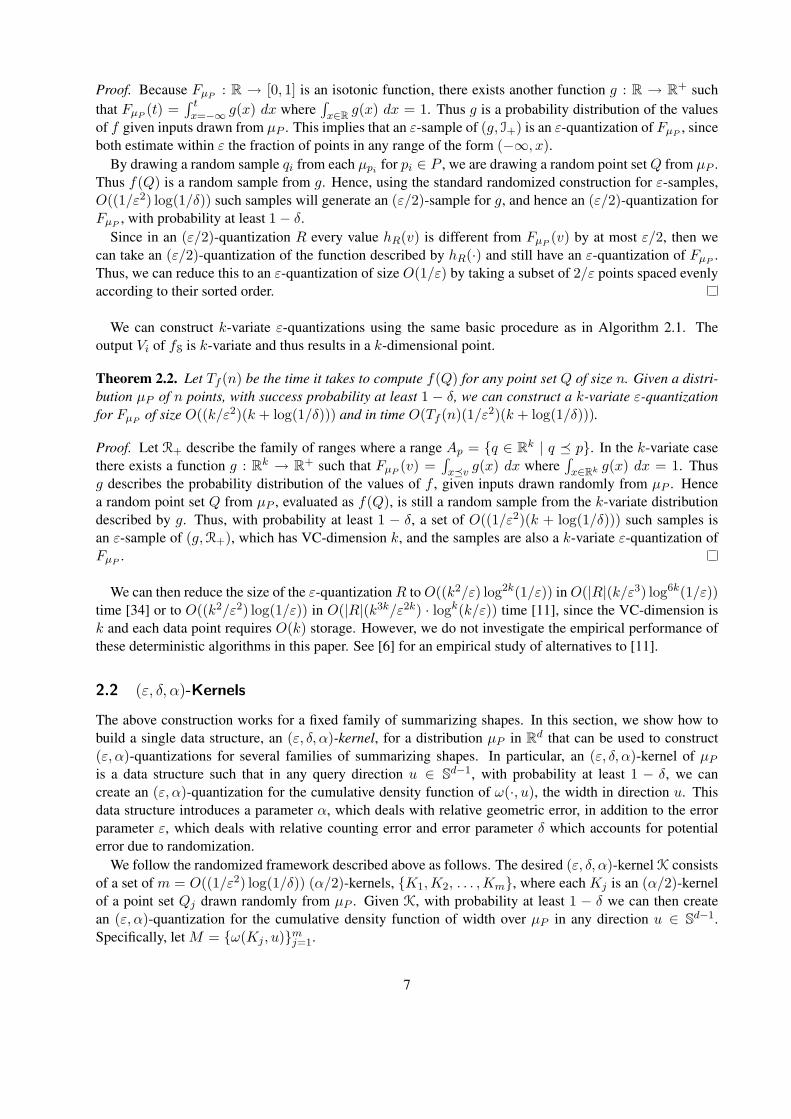
2.2 (ε, δ, α)-Kernels

The above construction works for a fixed family of summarizing shapes. In this section, we show how tobuild a single data structure, an (ε, δ, α)-kernel, for a distribution µP in Rd that can be used to construct(ε, α)-quantizations for several families of summarizing shapes. In particular, an (ε, δ, α)-kernel of µP

is a data structure such that in any query direction u ∈ Sd−1, with probability at least 1 − δ, we cancreate an (ε, α)-quantization for the cumulative density function of ω(·, u), the width in direction u. Thisdata structure introduces a parameter α, which deals with relative geometric error, in addition to the errorparameter ε, which deals with relative counting error and error parameter δ which accounts for potentialerror due to randomization.

We follow the randomized framework described above as follows. The desired (ε, δ, α)-kernel K consistsof a set of m = O((1/ε2) log(1/δ)) (α/2)-kernels, {K1,K2, . . . ,Km}, where each Kj is an (α/2)-kernelof a point set Qj drawn randomly from µP . Given K, with probability at least 1 − δ we can then createan (ε, α)-quantization for the cumulative density function of width over µP in any direction u ∈ Sd−1.Specifically, let M = {ω(Kj , u)}m

j=1.

7

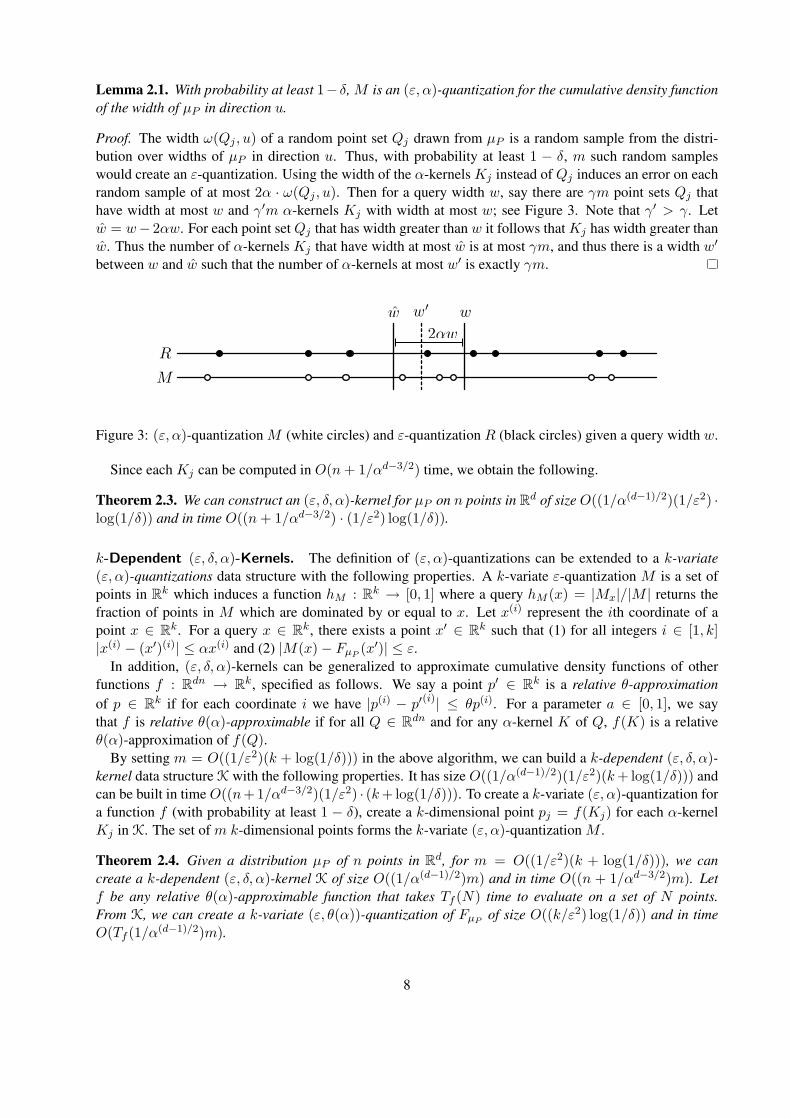
Lemma 2.1. With probability at least 1− δ, M is an (ε, α)-quantization for the cumulative density functionof the width of µP in direction u.

Proof. The width ω(Qj , u) of a random point set Qj drawn from µP is a random sample from the distri-bution over widths of µP in direction u. Thus, with probability at least 1 − δ, m such random sampleswould create an ε-quantization. Using the width of the α-kernels Kj instead of Qj induces an error on eachrandom sample of at most 2α · ω(Qj , u). Then for a query width w, say there are γm point sets Qj thathave width at most w and γ′m α-kernels Kj with width at most w; see Figure 3. Note that γ′ > γ. Letw = w− 2αw. For each point set Qj that has width greater than w it follows that Kj has width greater thanw. Thus the number of α-kernels Kj that have width at most w is at most γm, and thus there is a width w′

between w and w such that the number of α-kernels at most w′ is exactly γm.

ww!

M

R

w

2!w

Figure 3: (ε, α)-quantization M (white circles) and ε-quantization R (black circles) given a query width w.

Since each Kj can be computed in O(n + 1/αd−3/2) time, we obtain the following.

Theorem 2.3. We can construct an (ε, δ, α)-kernel for µP on n points in Rd of size O((1/α(d−1)/2)(1/ε2) ·log(1/δ)) and in time O((n + 1/αd−3/2) · (1/ε2) log(1/δ)).

k-Dependent (ε, δ, α)-Kernels. The definition of (ε, α)-quantizations can be extended to a k-variate(ε, α)-quantizations data structure with the following properties. A k-variate ε-quantization M is a set ofpoints in Rk which induces a function hM : Rk → [0, 1] where a query hM (x) = |Mx|/|M | returns thefraction of points in M which are dominated by or equal to x. Let x(i) represent the ith coordinate of apoint x ∈ Rk. For a query x ∈ Rk, there exists a point x′ ∈ Rk such that (1) for all integers i ∈ [1, k]|x(i) − (x′)(i)| ≤ αx(i) and (2) |M(x)− FµP (x′)| ≤ ε.

In addition, (ε, δ, α)-kernels can be generalized to approximate cumulative density functions of otherfunctions f : Rdn → Rk, specified as follows. We say a point p′ ∈ Rk is a relative θ-approximationof p ∈ Rk if for each coordinate i we have |p(i) − p′(i)| ≤ θp(i). For a parameter a ∈ [0, 1], we saythat f is relative θ(α)-approximable if for all Q ∈ Rdn and for any α-kernel K of Q, f(K) is a relativeθ(α)-approximation of f(Q).

By setting m = O((1/ε2)(k + log(1/δ))) in the above algorithm, we can build a k-dependent (ε, δ, α)-kernel data structure K with the following properties. It has size O((1/α(d−1)/2)(1/ε2)(k + log(1/δ))) andcan be built in time O((n+1/αd−3/2)(1/ε2) · (k +log(1/δ))). To create a k-variate (ε, α)-quantization fora function f (with probability at least 1 − δ), create a k-dimensional point pj = f(Kj) for each α-kernelKj in K. The set of m k-dimensional points forms the k-variate (ε, α)-quantization M .

Theorem 2.4. Given a distribution µP of n points in Rd, for m = O((1/ε2)(k + log(1/δ))), we cancreate a k-dependent (ε, δ, α)-kernel K of size O((1/α(d−1)/2)m) and in time O((n + 1/αd−3/2)m). Letf be any relative θ(α)-approximable function that takes Tf (N) time to evaluate on a set of N points.From K, we can create a k-variate (ε, θ(α))-quantization of FµP of size O((k/ε2) log(1/δ)) and in timeO(Tf (1/α(d−1)/2)m).

8

Proof. Let Q = {Q1, . . . , Qm} be the m points sets drawn randomly from µP and for the set K ={K1, . . . ,Km} let Kj be the α-kernel of Qj . Consider the probability distribution g describing the values off(Q) where Q is drawn randomly from µP . The set of m k-dimensional points {w1 = f(Q1), . . . , wm =f(Qm)} describes an ε-sample of (g,R+) and hence also an ε-quantization of FµP . We claim the set{w′

1 = f(K1), . . . , w′m = f(Km)} forms an (ε, α)-quantization of FµP .

For a query point w ∈ Rk, let γm point sets from Q produce a value wj = f(Qj) such that wj � w,and let γ′m point sets from K produce a value w′

j = f(Kj) such that w′j � w. Note that γ′ > γ. Let

w = w − θ(α)w; more specifically, for each coordinate w(i) of w, w(i) = w(i) − θ(α)w(i). Because f isrelative θ(α)-approximable, for each point set Qj ∈ Q such that wj � w, then w′

j � w. Thus, the number ofpoint sets such that f(Kj) � w is at most γm, and hence there is a point w′ between w and w such that thefraction of sampled point sets such that f(Kj) � w′ is exactly γ, and hence is within ε of the true fractionof point sets sampled from µP with probability at least 1− δ.

To name a few examples, the width and diameter are relative 2α-approximable functions, thus the resultsapply directly with k = 1. The radius of the minimum enclosing ball is relative 4α-approximable withk = 1. The d directional widths of the minimum perimeter or minimum volume axis-aligned rectangle isrelative 2α-approximable with k = d.

Remark 2.1. If an (ε, δ, α)-kernel is used for one query, it is correct with probability at least 1 − δ, andif it is used for another query, it is also correct with probability at least 1 − δ. Although there is probablysome dependence between these two quantities, it is not easy to prove in general, hence we only claim theprobability they are both correct is at least (1 − δ)2. We can increase this back to 1 − δ for k queries bysetting m = O((1/ε2)(k + log(1/δ))), but we need to specify k in advance. If we had a deterministicconstruction to create an (ε, 0, α)-kernel this would not be a problem, and we could, say, guarantee an(ε, α)-quantization for width in all directions simultaneously. However, this appears to be a much moredifficult problem.

Other coresets. In a similar fashion, coresets of a point set distribution µP can be formed using othercoresets for other problems on discrete point sets. For instance, sample m = O((1/ε2) log(1/δ)) pointssets {P1, . . . , Pm} each from µP and then store α-samples {Q1 ⊆ P1, . . . , Qm ⊆ Pm} of each. (If we userandom sampling in the second set, then not all distributions µpi need to be sampled for each Pj in the firstround.) This results in an (ε, δ, α)-sample of µP , and can, for example, be used to construct (with probability1− δ) an (ε, α)-quantization for the fraction of points expected to fall in a query disk. Similar constructionscan be done for other coresets, such as ε-nets [22], k-center [4, 21], or smallest enclosing ball [8].

2.3 Shape Inclusion Probabilities

We can also use a variation of Algorithm 2.1 to construct ε-shape inclusion probability functions. For apoint set Q ⊂ Rd, let the summarizing shape SQ = S(Q) be from some geometric family S so (Rd, S)has bounded VC-dimension ν. We randomly sample m point sets Q = {Q1, . . . , Qm} each from µP andthen find the summarizing shape SQj = S(Qj) (e.g. minimum enclosing ball) of each Qj . Let this set ofshapes be SQ. If there are multiple shapes from S which are equally optimal (as can happen degenerately3

with, for example, minimum width slabs), choose one of these shapes at random. For a set of shapesS′ ⊆ S, let S′p ⊆ S′ be the subset of shapes that contain p ∈ Rd. We store SQ and evaluate a query pointp ∈ Rd by counting what fraction of the shapes the point is contained in, specifically returning |SQ

p |/|SQ| inO(ν|SQ|) = O(νm) time. In some cases, this evaluation can be sped up with point location data structures.

3In cases such as the smallest enclosing ball under the `1 distance, there may be multiple possible optimal shapes, non-degenerately. We can either choose one at random, or redefine the summarizing shape as the union of all such shapes.

9

Theorem 2.5. Consider a family of summarizing shapes S where (Rd, S) has VC-dimension ν and whereit takes TS(n) time to determine the summarizing shape S(Q) for any point set Q ⊂ Rd of size n. For adistribution µP of a point set of size n, with probability at least 1− δ, we can construct an ε-sip function ofsize O((ν/ε2)(2ν+1 + log(1/δ))) and in time O(TS(n)(1/ε2) log(1/δ)).

Proof. If (Rd, S) has VC-dimension ν, then the dual range space (S, P ∗) has VC-dimension ν ′ ≤ 2ν+1,where P ∗ is all subsets Sp ⊆ S, for any p ∈ Rd, such that Sp = {S ∈ S | p ∈ S}. Using the abovealgorithm, sample m = O((1/ε2)(ν ′ + log(1/δ))) point sets Q from µP and generate the m summarizingshapes SQ. Each shape is a random sample from S according to µP , and thus SQ is an ε-sample of (S, P ∗).

Let wµP (S), for S ∈ S, be the probability that S is the summarizing shape of a point set Q drawnrandomly from µP . For any S′ ⊆ P ∗, let WµP (S′) =

∫S∈S′ wµP (S) be the probability that some shape from

the subset S′ is the summarizing shape of Q drawn from µP .We approximate the sip function at p ∈ Rd by returning the fraction |SQ

p |/m. The true answer to the sip

function at p ∈ Rd is WµP (Sp). Since SQ is an ε-sample of (S, P ∗), then with probability at least 1− δ∣∣∣∣∣ |SQp |

m− WµP (Sp)

1

∣∣∣∣∣ =

∣∣∣∣∣ |SQp |

|SQ|− WµP (Sp)

WµP (P ∗)

∣∣∣∣∣ ≤ ε.

Since for the family of summarizing shapes S the range space (Rd, S) has VC-dimension ν, each can bestored using that much space.

Using deterministic techniques [11] the size can then be reduced to O(2ν+1(ν/ε2) · log(1/ε)) in timeO((23(ν+1) · (ν/ε2) log(1/ε))2

ν+1 · 23(ν+1)(ν/ε2) log(1/δ)).

(a) (b) (c) (d)

Figure 4: The shape inclusion probability for the smallest enclosing ball (a,b) or smallest enclosing axis-aligned rectangle (c,d), for points uniformly distributed inside the circles (a,c) or normally distributed aroundcircle centers with standard deviation given by radii (b,d).

Representing ε-sip functions by isolines. Shape inclusion probability functions are density functions.One convenient way of visually representing a density function in R2 is by drawing the isolines. A γ-isolineis a collection of closed curves bounding a region of the plane where the density function is greater than γ.

In each part of Figure 4 a set of 5 circles correspond to points with a probability distribution. In part(a,c) the probability distribution is uniform over the inside of the circles. In part (b,d) it is drawn from amultivariate Gaussian distribution, where the standard deviation is given by the radius or the circle. Wegenerate ε-sip functions for the smallest enclosing ball in Figure 4(a,b) and for the smallest axis-alignedbounding box in Figure 4(c,d).

10

In all figures we draw approximations of {.9, .7, .5, .3, .1}-isolines. These drawing are generated byrandomly selecting m = 5000 (Figure 4(a,b)) or m = 25000 (Figure 4(c,d)) shapes, counting the numberof inclusions at different points in the plane and interpolating to get the isolines. The innermost and darkestregion has probability > 90%, the next one probability > 70%, etc., the outermost region has probability< 10%.

When µP describes the distribution for n points and n is large, then isolines are generally connected forconvex summarizing shapes. In fact, in O(n) time we can create a point which is contained in the convexhull of a point set sampled from µP with high probability. Specifics are discussed in Appendix A.

3 Measuring the Error

We have established asymptotic bounds of O((1/ε2)(ν + log(1/δ)) random samples for constructing ε-quantizations and ε-sip functions. In this section we empirically demonstrate that the constant hidden by thebig-O notation is approximately 0.5, indicating that these algorithms are indeed quite practical. Additionally,we show that we can reduce the size of ε-quantizations to 2/ε without sacrificing accuracy and with only afactor 4 increase in the runtime. We also briefly compare the (ε, α)-quantizations produced with (ε, δ, α)-kernels to ε-quantizations. We show that the (ε, δ, α)-kernels become useful when the number of uncertainpoints becomes large, i.e. exceeding 1000.

Univariate ε-quantizatons. We consider a set of n = 50 sample points in R3 chosen randomly from theboundary of a cylinder piece of length 10 and radius 1. We let each point represent the center of 3-variateGaussian distribution with standard deviation 2 to represent the probability distribution of an uncertain point.This set of distributions describes an uncertain point set µP : R3n → R+.

We want to estimate three statistics on µP : diam, the diameter of the point set; dwid, the width of thepoints set in a direction that makes an angle of 75◦ with the cylinder axis; and seb2, the radius of the smallestenclosing ball (using code from Bernd Gartner [17]). We can create ε-quantizations using our randomizedalgorithm with m samples from µP , where the value of m is from the set {16, 64, 256, 1024, 4096}.

We would like to evaluate the ε-quantizations versus the ground truth function FµP ; however, it is notclear how to evaluate FµP . Instead, we create another ε-quantization Q with η = 100000 samples from µP ,and treat this as if it were the ground truth. To evaluate each sample ε-quantization R versus Q we find themaximum deviation (i.e. d∞(R,Q) = maxq∈R |hR(q) − hQ(q)|) with h defined respect to diam, dwid, orseb2. This can be done by for each value r ∈ R evaluating |hR(r)− hQ(r)| and |(hR(r)− 1/|R|)− hQ(r)|and returning the maximum of both values over all r ∈ R. Since, for two consecutive points qi, qi+1 ∈ R,the value of hQ must increase monotonically between these values, so the maximum deviation must occurat the boundary of some such interval between consecutive points. This maximum error can be calculatedin O(η + m) time by scanning the two data structures in parallel and maintaining running sums (or inO(m log η) time using a binary tree on Q).

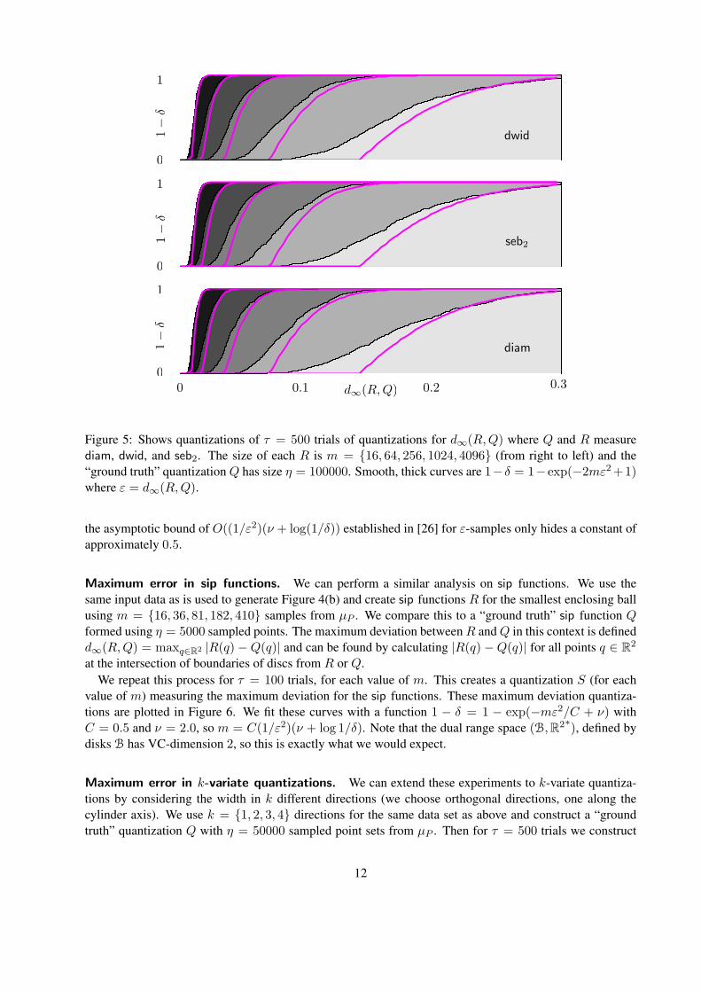
Given a fixed “ground truth” quantization Q we repeat this process for τ = 500 trials of R, each returninga d∞(R,Q) value. The set of these τ maximum deviations values results in another quantization S for eachof diam, dwid, and seb2. Intuitively, the maximum deviation quantization S describes the sample probabilitythat d∞(R,Q) will be less than some query value. These are plotted in Figure 5 for each value of m.

Note that the maximum deviation quantizations S are similar for all three statistics, and thus we can usethese plots to estimate 1 − δ, the sample probability that d∞(R,Q) ≤ ε, given a value m. We can fit thisfunction as approximately 1− δ = 1− exp(−mε2/C + ν) with C = 0.5 and ν = 1.0. Thus solving for min terms of ε, ν, and δ reveals: m = C(1/ε2)(ν + log(1/δ)). 4 This indicates that the big-O notation for

4Actually the function 1− δ = 1− exp(ε(p

m/C − ν)2) and m = C(1/ε2)(ν +p

log(1/δ))2 with C = 0.3 and ν = 0.75fits the data much better but does not match the asymptotic bound as directly.

11

d!(R,Q)0

1

1

1

0

0

1!

!1!

!1!

!

0 0.30.20.1

seb2

dwid

diam

Figure 5: Shows quantizations of τ = 500 trials of quantizations for d∞(R,Q) where Q and R measurediam, dwid, and seb2. The size of each R is m = {16, 64, 256, 1024, 4096} (from right to left) and the“ground truth” quantization Q has size η = 100000. Smooth, thick curves are 1−δ = 1−exp(−2mε2 +1)where ε = d∞(R,Q).

the asymptotic bound of O((1/ε2)(ν + log(1/δ)) established in [26] for ε-samples only hides a constant ofapproximately 0.5.

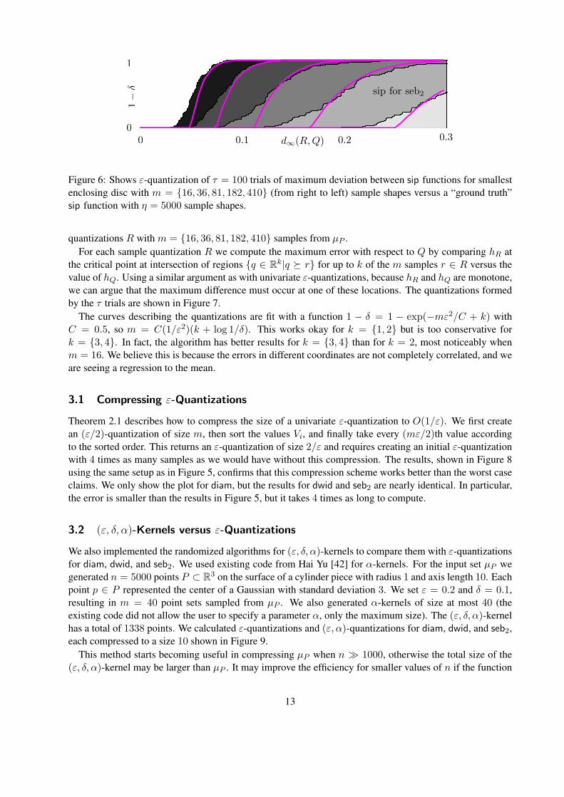
Maximum error in sip functions. We can perform a similar analysis on sip functions. We use thesame input data as is used to generate Figure 4(b) and create sip functions R for the smallest enclosing ballusing m = {16, 36, 81, 182, 410} samples from µP . We compare this to a “ground truth” sip function Qformed using η = 5000 sampled points. The maximum deviation between R and Q in this context is definedd∞(R,Q) = maxq∈R2 |R(q)−Q(q)| and can be found by calculating |R(q)−Q(q)| for all points q ∈ R2

at the intersection of boundaries of discs from R or Q.We repeat this process for τ = 100 trials, for each value of m. This creates a quantization S (for each

value of m) measuring the maximum deviation for the sip functions. These maximum deviation quantiza-tions are plotted in Figure 6. We fit these curves with a function 1 − δ = 1 − exp(−mε2/C + ν) withC = 0.5 and ν = 2.0, so m = C(1/ε2)(ν + log 1/δ). Note that the dual range space (B, R2∗), defined bydisks B has VC-dimension 2, so this is exactly what we would expect.

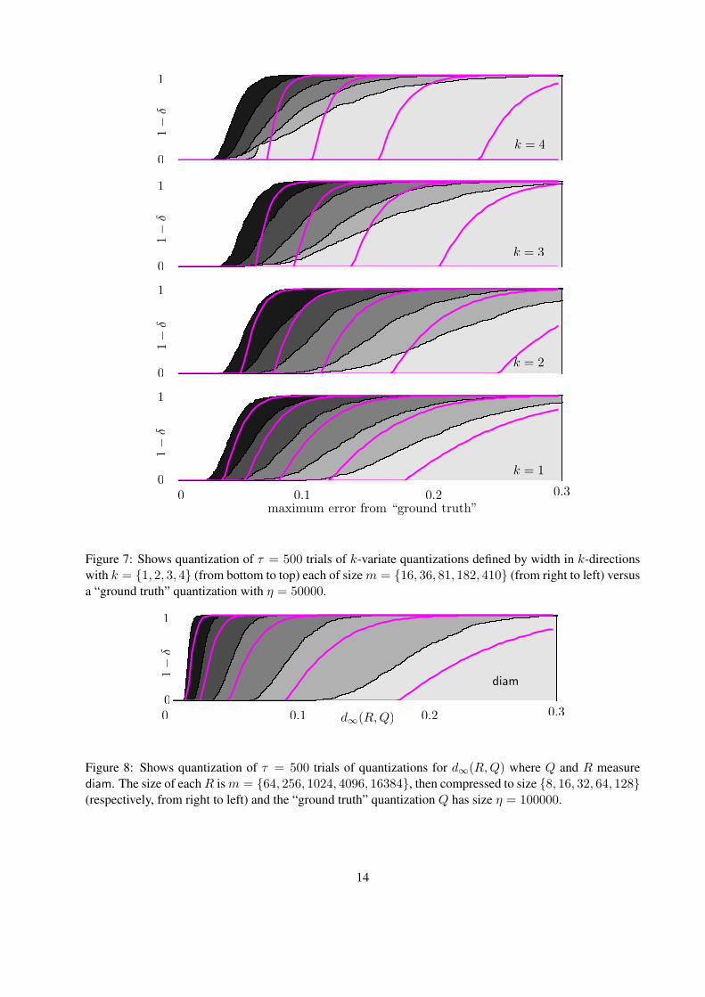
Maximum error in k-variate quantizations. We can extend these experiments to k-variate quantiza-tions by considering the width in k different directions (we choose orthogonal directions, one along thecylinder axis). We use k = {1, 2, 3, 4} directions for the same data set as above and construct a “groundtruth” quantization Q with η = 50000 sampled point sets from µP . Then for τ = 500 trials we construct

12

d!(R,Q)0

1

1!

!0 0.30.20.1

sip for seb2

Figure 6: Shows ε-quantization of τ = 100 trials of maximum deviation between sip functions for smallestenclosing disc with m = {16, 36, 81, 182, 410} (from right to left) sample shapes versus a “ground truth”sip function with η = 5000 sample shapes.

quantizations R with m = {16, 36, 81, 182, 410} samples from µP .For each sample quantization R we compute the maximum error with respect to Q by comparing hR at

the critical point at intersection of regions {q ∈ Rk|q � r} for up to k of the m samples r ∈ R versus thevalue of hQ. Using a similar argument as with univariate ε-quantizations, because hR and hQ are monotone,we can argue that the maximum difference must occur at one of these locations. The quantizations formedby the τ trials are shown in Figure 7.

The curves describing the quantizations are fit with a function 1 − δ = 1 − exp(−mε2/C + k) withC = 0.5, so m = C(1/ε2)(k + log 1/δ). This works okay for k = {1, 2} but is too conservative fork = {3, 4}. In fact, the algorithm has better results for k = {3, 4} than for k = 2, most noticeably whenm = 16. We believe this is because the errors in different coordinates are not completely correlated, and weare seeing a regression to the mean.

3.1 Compressing ε-Quantizations

Theorem 2.1 describes how to compress the size of a univariate ε-quantization to O(1/ε). We first createan (ε/2)-quantization of size m, then sort the values Vi, and finally take every (mε/2)th value accordingto the sorted order. This returns an ε-quantization of size 2/ε and requires creating an initial ε-quantizationwith 4 times as many samples as we would have without this compression. The results, shown in Figure 8using the same setup as in Figure 5, confirms that this compression scheme works better than the worst caseclaims. We only show the plot for diam, but the results for dwid and seb2 are nearly identical. In particular,the error is smaller than the results in Figure 5, but it takes 4 times as long to compute.

3.2 (ε, δ, α)-Kernels versus ε-Quantizations

We also implemented the randomized algorithms for (ε, δ, α)-kernels to compare them with ε-quantizationsfor diam, dwid, and seb2. We used existing code from Hai Yu [42] for α-kernels. For the input set µP wegenerated n = 5000 points P ⊂ R3 on the surface of a cylinder piece with radius 1 and axis length 10. Eachpoint p ∈ P represented the center of a Gaussian with standard deviation 3. We set ε = 0.2 and δ = 0.1,resulting in m = 40 point sets sampled from µP . We also generated α-kernels of size at most 40 (theexisting code did not allow the user to specify a parameter α, only the maximum size). The (ε, δ, α)-kernelhas a total of 1338 points. We calculated ε-quantizations and (ε, α)-quantizations for diam, dwid, and seb2,each compressed to a size 10 shown in Figure 9.

This method starts becoming useful in compressing µP when n � 1000, otherwise the total size of the(ε, δ, α)-kernel may be larger than µP . It may improve the efficiency for smaller values of n if the function

13

maximum error from “ground truth”

0

1

1

1

0

0

1!

!1!

!1!

!

0 0.30.20.1

k = 3

k = 1

k = 2

1

01!

!k = 4

Figure 7: Shows quantization of τ = 500 trials of k-variate quantizations defined by width in k-directionswith k = {1, 2, 3, 4} (from bottom to top) each of size m = {16, 36, 81, 182, 410} (from right to left) versusa “ground truth” quantization with η = 50000.

0

1

1!

!

0 0.30.20.1

diam

d!(R,Q)

Figure 8: Shows quantization of τ = 500 trials of quantizations for d∞(R,Q) where Q and R measurediam. The size of each R is m = {64, 256, 1024, 4096, 16384}, then compressed to size {8, 16, 32, 64, 128}(respectively, from right to left) and the “ground truth” quantization Q has size η = 100000.

14

!!

6.8176.535

!!

9.343 10.642

!!

13.017 13.633(a) (b) (c)

Figure 9: (ε, α)-quantization (white points) and ε-quantization (black points) for (a) seb2, (b) dwid, and (c)diam.

f : µP → R that the quantization is approximating is expensive to compute (e.g. it takes O(nρ) time forρ > 1). We point the curious reader to [42] to validate the practicality of α-kernels.

Acknowledgements

We would like to thank Pankaj K. Agarwal for many helpful discussions. This research was partially sup-ported by the Netherlands Organisation for Scientific Research (NWO) through the project GOGO.

References

[1] Charu C. Agarwal and Philip S. Yu, editors. Privacy Preserving Data Mining: Models and Algorithms.Springer, 2008.

[2] Pankaj K. Agarwal, Sariel Har-Peled, and Kasturi Varadarajan. Geometric approximations via coresets.Current Trends in Combinatorial and Computational Geometry (E. Welzl, ed.), 2007.

[3] Pankaj K. Agarwal, Sariel Har-Peled, and Kasturi R. Varadarajan. Approximating extent measure ofpoints. Journal of ACM, 51(4):2004, 2004.

[4] Pankaj K. Agarwal, Cecilia M. Procopiuc, and Kasturi R. Varadarajan. Approximation algorithms fork-line center. In Proceedings 10th Annual European Symposium on Algorithms, pages 54–63, 2002.

[5] Rakesh Agarwal and Ramakrishnan Srikant. Privacy-preserving data mining. ACM SIGMOD Record,29:439–450, 2000.

[6] Huseyin Akcan, Alex Astashyn, and Herve Bronnimann. Deterministic algorithms for sampling countdata. Data & Knowledge Engineering, 64(2):405–418, February 2008.

[7] Deepak Bandyopadhyay and Jack Snoeyink. Almost-Delaunay simplices: Nearest neighbor relationsfor imprecise points. In ACM-SIAM Symp on Discrete Algorithms, pages 403–412, 2004.

[8] Mihai Badoiu and Ken Clarkson. Smaller core-sets for balls. In Proceedings of the 14th AnnualACM-SIAM Symposium on Discrete Algorithms, 2003.

[9] Timothy Chan. Faster core-set constructions and data-stream algorithms in fixed dimensions. Compu-tational Geometry: Theory and Applications, 35:20–35, 2006.

[10] Timothy Chan. Dynamic coresets. In Proceedings of the 24th ACM Symposium on ComputationalGeometry, pages 1–9, 2008.

15

[11] Bernard Chazelle and Jiri Matousek. On linear-time deterministic algorithms for optimization prob-lems in fixed dimensions. Journal of Algorithms, 21:579–597, 1996.

[12] Reynold Cheng, Jichuan Chen, Mohamed Mokbel, and Chi-Yin Chow. Probability verifiers: Evaluat-ing constrainted nearest-neighbor queries over uncertain data. In Proceedings Interantional Conferenceon Data Engineering, 2008.

[13] Reynold Cheng, Dmitri V. Kalashnikov, and Sunil Prabhakar. Evaluating probabilitic queries overimprecise data. In Proceedings 2003 ACM SIGMOD International Conference on Management ofData, 2003.

[14] Kenneth L. Clarkson, David Eppstein, Gary L. Miller, Carl Sturtivant, and Shang-Hua Teng. Approx-imating center points with iterative Radon points. International Journal of Computational Geometryand Applications, 6:357–377, 1996.

[15] Amol Deshpande, Carlos Guestrin, Samuel R. Madden, Joseph M. Hellerstein, and Wei Hong. Model-driven data acquisition in sensor networks. In Proceedings 13th International Conference on VeryLarge Data Bases, 2004.

[16] Austin Eliazar and Ronald Parr. Dp-slam 2.0. In Proceedings 2004 IEEE International Conference onRobotics and Automation, 2004.

[17] Bernd Gartner. Fast and robust smallest enclosing balls. In Proceedings 7th Annual European Sympo-sium on Algorithms, volume LNCS 1643, pages 325–338, 1999.

[18] Leonidas J. Guibas, D. Salesin, and J. Stolfi. Epsilon geometry: building robust algorithms fromimprecise computations. In Proc. 5th Annu. ACM Sympos. Comput. Geom., pages 208–217, 1989.

[19] Leonidas J. Guibas, D. Salesin, and J. Stolfi. Constructing strongly convex approximate hulls withinaccurate primitives. Algorithmica, 9:534–560, 1993.

[20] R. H. Guting and M. Schneider. Moving Object Databases. Morgan Kaufmann, San Francisco, 2005.

[21] Sariel Har-Peled. No coreset, no cry. In Proceedings 24th Conference on Foundations of SoftwareTechnology and Theoretical Computer Science, 2004.

[22] David Haussler and Emo Welzl. epsilon-nets and simplex range queries. Discrete and ComputationalGeometry, 2:127–151, 1987.

[23] Martin Held and Joseph S. B. Mitchell. Triangulating input-constrained planar point sets. InformationProcessing Letters, 109:54–56, 2008.

[24] Dmitri V. Kalashnikov, Yiming Ma, Sharad Mehrotra, and Ramaswamy Hariharan. Index for fastretreival of uncertain spatial point data. In Proceedings 16th ACM SIGSPATIAL Interanational Con-ference on Advances in Geographic Information Systems, 2008.

[25] Heinrich Kruger. Basic measures for imprecise point sets in Rd. Master’s thesis, Utrecht University,2008.

[26] Yi Li, Philip M. Long, and Aravind Srinivasan. Improved bounds on the samples complexity of learn-ing. Journal of Computer ans System Science, 62:516–527, 2001.

[27] T. M. Lillesand, R. W. Kiefer, and J. W. Chipman. Remote Sensing and Image Interpretaion. JohnWiley & Sons, 2004.

16

[28] Maarten Loffler and Jack Snoeyink. Delaunay triangulations of imprecise points in linear time afterpreprocessing. In Proc. 24th Sympoium on Computational Geometry, pages 298–304, 2008.

[29] Jiri Matousek. Approximations and optimal geometric divide-and-conquer. In Proceedings of the 23rdAnnual ACM Symposium on Theory of Computing, pages 505–511, 1991.

[30] Jiri Matousek. Geometric Discrepancy; An Illustrated Guide, volume 18 of Algorithms and Combina-torics. Springer, 1999.

[31] Jiri Matousek, Emo Welzl, and Lorenz Wernisch. Discrepancy and approximations for bounded vc-dimension. Combinatorica, 13(4):455–466, 1993.

[32] T. Nagai and N. Tokura. Tight error bounds of geometric problems on convex objects with imprecisecoordinates. In Jap. Conf. on Discrete and Comput. Geom., LNCS 2098, pages 252–263, 2000.

[33] Y. Ostrovsky-Berman and L. Joskowicz. Uncertainty envelopes. In Abstracts 21st European Workshopon Comput. Geom., pages 175–178, 2005.

[34] Jeff M. Phillips. Algorithms for ε-approximations of terrains. In Proceedings 35th InternationalColloquium on Automata, Languages, and Programming, 2008. arXiV 0801.2793.

[35] Shobha Potluri, Anthony K. Yan, James J. Chou, Bruce R. Donald, and Chris Baily-Kellogg. Structuredetermination of symmetric homo-oligomers by complete search of symmetry configuration space,using nmr restraints and van der Waals packing. Proteins, 65:203–219, 2006.

[36] R. Rado. A theorem on general measure. Journal of the London Mathematical Society, 21:291–300,1947.

[37] S. Shekhar and S. Chawla. Spatial Databases: A Tour. Pearsons, 2001.

[38] Yufei Tao, Reynold Cheng, Xiaokui Xiao, Wang Kay Ngai, Ben Kao, and Sunil Prabhakar. Indexingmutli-dimensional uncertain data with arbitrary probability density functions. In Proceedings 31st VeryLarge Data Bases Conference, 2005.

[39] Sebastian Thrun. Robotic mapping: A survey. Exploring Artificial Intelligence in the New Millenium,2002.

[40] Marc van Kreveld and Maarten Loffler. Largest bounding box, smallest diameter, and related problemson imprecise points. accepted for publication in Computational Geometry: Theory and Applications.

[41] Vladimir Vapnik and Alexey Chervonenkis. On the uniform convergence of relative frequencies ofevents to their probabilities. Theory of Probability and its Applications, 16:264–280, 1971.

[42] Hai Yu, Pankaj K. Agarwal, Raghunath Poreddy, and Kasturi R. Varadarajan. Practical methods forshape fitting and kinetic data structures using coresets. In Proceedings 20th Annual Symposium onComputational Geometry, 2004.

A A center point for µP .

We can create a point q ∈ Rd that is in the convex hull of a sampled point set Q from µP with highprobability. This implies that for any summarizing shape that contains the convex hull, q is also containedin that summarizing shape. For a point set P ⊂ Rd, a β-center point is a point q ∈ Rd, such that any closed

17

halfspace that contains q also contains at least 1/β fraction points of all points in P . It is known that forany discrete point set a (d + 1)-center point always exists [36]. Let H be the family of subsets defined byhalfspaces. For a point set P of size n, a (2d + 2)-center point can be created in O(d5d+3 logd d) time [14]by first creating an (1/(2d + 2))-sample of (P,H), and then running a brute force algorithm. Because thefirst step is creating an ε-sample, this can be extended to Lebesgue-measureable sets such as probabilitydistributions as well.

We use the following algorithm:

1. Create a (2d + 2)-center point pi for each µpi . Let the set be P .

2. Create (2d + 2)-center point q of P .

For d constant, the algorithm runs in O(n) time because we can create (2d+2)-center points a total of n+1times, and each takes O(1) time.

Lemma A.1. Given a distribution of a point set µP (such that each point distribution is polygonally ap-proximable) of n points in Rd, there is an O(n) time algorithm to create a point q that will be in the convexhull of a point set drawn from µP with probability at least 1− (e1/(2d+2)2)n.

Proof. Because pi is a (2d+2)-center point of µpi , any halfspace that contains pi on its boundary (and doesnot contain q) has probability at least 1/(2d + 2) of containing a point randomly drawn from µpi . Also,because q is a (2d + 2)-center point of P , for any direction u ∈ Sd−1 there are at least n/(2d + 2) pointspi from P for which 〈q, u〉 ≤ 〈pi, u〉. Thus, if a point qi is drawn from µpi such that 〈q, u〉 ≤ 〈pi, u〉 thenthe probability that 〈q, u〉 ≤ 〈qi, u〉 is at least 1/(2d + 2). Hence, the probability that there is a separatinghalfspace between q and the convex hull of Q (where the halfspace is orthogonal to some direction u) is atmost

(1− 1/(2d + 2))n/(2d+2) = ((1− 1/(2d + 2))1/(2d+2))n ≤ (e1/(2d+2)2)n.

Theorem A.1. For a set of m < n point sets drawn i.i.d. from µP , it follows that q is in each of the mconvex hulls for each point sets with high probability (specifically with probability ≥ 1−m(e1/(2d+2)2)n).

Proof. Let β = e1/(2d+2)2 . For any one point set the probability that q is contained in the convex hull isat least 1 − βn. By the union bound, the probability that it is contained in all m convex hulls is at least(1− βn)m = 1−mβn +

(m2

)β2n −

(m3

)β3n + . . .. Since n > m, the sum of all terms after the first two in

the expansion increase the probability.

We say a family of shapes S is convex if S(P ) ∈ S contains the convex hull of P and S(P ) is always aconvex set. When S is convex, then for any point q, the line segment qq is completely contained in S(P ) ifand only if q ∈ S(P ). Thus, given a set of m summarizing shapes, for every boundary of a summarizingshape qq crosses, q is outside that summarizing shape. This implies the following corollary.

Corollary A.1. Consider a distribution µP of point sets of size n, a convex family of shapes S inducing asip function sS on µP , and a positive integer m < n. For γ ≤ 1 − 1/m the subset of Rd inside of theγ-isoline of sS, exists, is connected, and is star-shaped with high probability, specifically with probability atleast 1−m(e1/(2d+2)2)n.

18