Embed Size (px)
Citation preview
Shape Factors for the Pseudo-Steady State Flow in Fractured
Hydrocarbon Wells of Various Drainage Area Geometries
by
Ankush Sharma
A Thesis Presented in Partial Fulfillmentof the Requirements for the Degree
Master of Science
Approved May 2017 by theGraduate Supervisory Committee:
Kangping Chen, Co-ChairMatthew Green, Co-Chair
Heather Emady
ARIZONA STATE UNIVERSITY
August 2017
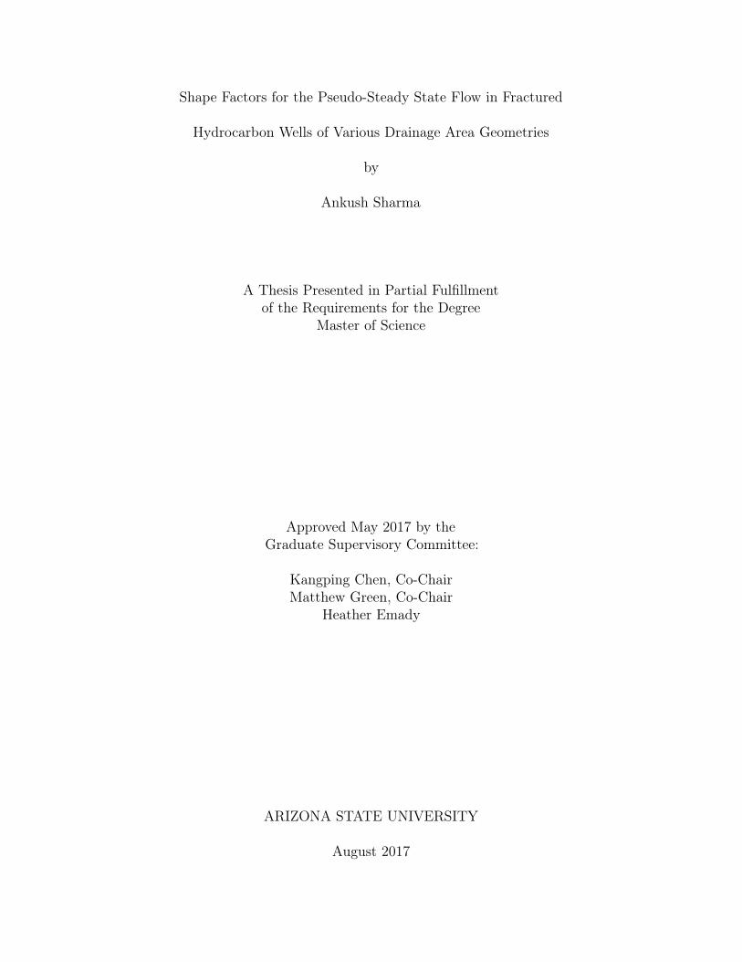
ABSTRACT
Pseudo-steady state (PSS) flow is an important time-dependent flow regime that
quickly follows the initial transient flow regime in the constant-rate production of
a closed boundary hydrocarbon reservoir. The characterization of the PSS flow
regime is of importance in describing the reservoir pressure distribution as well as the
productivity index (PI) of the flow regime. The PI describes the production potential
of the well and is often used in fracture optimization and production-rate decline
analysis. In 2016, Chen determined the exact analytical solution for PSS flow of a
fully penetrated vertically fractured well with finite fracture conductivity for reservoirs
of elliptical shape. The present work aimed to expand Chen’s exact analytical solution
to commonly encountered reservoirs geometries including rectangular, rhomboid,
and triangular by introducing respective shape factors generated from extensive
computational modeling studies based on an identical drainage area assumption. The
aforementioned shape factors were generated and characterized as functions for use
in spreadsheet calculations as well as graphical format for simplistic in-field look-up
use. Demonstrative use of the shape factors for over 20 additional simulations showed
high fidelity of the shape factor to accurately predict (mean average percentage error
remained under 1.5 %) the true PSS constant by modulating Chen’s solution for
elliptical reservoirs. The methodology of the shape factor generation lays the ground
work for more extensive and specific shape factors to be generated for cases such as
non-concentric wells and other geometries not studied.
i

DEDICATION
This work is dedicated to my loving parents and sisters who constantly support
me in all aspects of my life including my academic endeavors.
ii

ACKNOWLEDGMENTS
Major acknowledgment is given to Dr. Kang Ping Chen for endlessly guiding my
research over the past two years and always finding time to aide me in my professional
pursuits. Dr. Chen not only made the present work possible but also pushed me
farther than I could have gone solely, and aided me in sharing my work.
Further acknowledgment is given to Dr. Matthew Green and Dr. Heather Emady
for their attentive support and guidance on the present work and their continued
willingness to promptly aide me in completing my research.
iii
TABLE OF CONTENTS
Page
LIST OF TABLES . . . . . . . . . . . . . . . . . . . . . . . . . . . . . . . . . . . . . . . . . . . . . . . . . . . . . . . . vi
LIST OF FIGURES . . . . . . . . . . . . . . . . . . . . . . . . . . . . . . . . . . . . . . . . . . . . . . . . . . . . . . . vii
CHAPTER
1 INTRODUCTION . . . . . . . . . . . . . . . . . . . . . . . . . . . . . . . . . . . . . . . . . . . . . . . . . 1
1.1 Background . . . . . . . . . . . . . . . . . . . . . . . . . . . . . . . . . . . . . . . . . . . . . . . . . . . 1
1.2 Pseudo-Steady State . . . . . . . . . . . . . . . . . . . . . . . . . . . . . . . . . . . . . . . . . . . 3
1.3 Pseudo-Steady State Characterization . . . . . . . . . . . . . . . . . . . . . . . . . . 6
1.4 Purpose . . . . . . . . . . . . . . . . . . . . . . . . . . . . . . . . . . . . . . . . . . . . . . . . . . . . . . 9
2 METHODOLOGY . . . . . . . . . . . . . . . . . . . . . . . . . . . . . . . . . . . . . . . . . . . . . . . . . 10
2.1 Overview . . . . . . . . . . . . . . . . . . . . . . . . . . . . . . . . . . . . . . . . . . . . . . . . . . . . . 10
2.2 COMSOL Multiphysics Modeling . . . . . . . . . . . . . . . . . . . . . . . . . . . . . . . 10
2.2.1 Rectangular Reservoirs . . . . . . . . . . . . . . . . . . . . . . . . . . . . . . . . . . . 13
2.2.2 Rhomboid Reservoirs . . . . . . . . . . . . . . . . . . . . . . . . . . . . . . . . . . . . 14
2.2.3 Triangular Reservoirs . . . . . . . . . . . . . . . . . . . . . . . . . . . . . . . . . . . . 15
2.3 Post-Processing . . . . . . . . . . . . . . . . . . . . . . . . . . . . . . . . . . . . . . . . . . . . . . . 15
3 RESULTS . . . . . . . . . . . . . . . . . . . . . . . . . . . . . . . . . . . . . . . . . . . . . . . . . . . . . . . . . 17
3.1 Rectangular Shape Factor . . . . . . . . . . . . . . . . . . . . . . . . . . . . . . . . . . . . . . 17
3.2 Rhomboid Shape Factor . . . . . . . . . . . . . . . . . . . . . . . . . . . . . . . . . . . . . . . 19
3.3 Triangular Shape Factor . . . . . . . . . . . . . . . . . . . . . . . . . . . . . . . . . . . . . . . 20
3.4 Demonstrative Use of Shape Factors . . . . . . . . . . . . . . . . . . . . . . . . . . . . 23
4 DISCUSSION . . . . . . . . . . . . . . . . . . . . . . . . . . . . . . . . . . . . . . . . . . . . . . . . . . . . . . 26
5 CONCLUSIONS . . . . . . . . . . . . . . . . . . . . . . . . . . . . . . . . . . . . . . . . . . . . . . . . . . . 28
5.1 Future Work . . . . . . . . . . . . . . . . . . . . . . . . . . . . . . . . . . . . . . . . . . . . . . . . . . 29
iv
CHAPTER Page
REFERENCES . . . . . . . . . . . . . . . . . . . . . . . . . . . . . . . . . . . . . . . . . . . . . . . . . . . . . . . 30
APPENDIX
A RECTANGULAR LOOK-UP TABLES . . . . . . . . . . . . . . . . . . . . . . . . . . . . . . 33
B RECTANGULAR SHAPE FACTOR CONFIDENCE INTERVALS . . . . 38
C RHOMBOID LOOK-UP TABLE . . . . . . . . . . . . . . . . . . . . . . . . . . . . . . . . . . . . 40
D TRIANGULAR LOOK-UP TABLE . . . . . . . . . . . . . . . . . . . . . . . . . . . . . . . . . 42
E CURVE FITTING STATISTICS . . . . . . . . . . . . . . . . . . . . . . . . . . . . . . . . . . . . 44
v
LIST OF TABLES
Table Page
1. COMSOL Multiphysics Parameters . . . . . . . . . . . . . . . . . . . . . . . . . . . . . . . . . . . . . . . 12
2. Shape Factor Equations . . . . . . . . . . . . . . . . . . . . . . . . . . . . . . . . . . . . . . . . . . . . . . . . . . 22
3. Rectangular (Ar = 4) Shape Factor Estimations . . . . . . . . . . . . . . . . . . . . . . . . . . . 23
4. Rhomboid Shape Factor Estimations. . . . . . . . . . . . . . . . . . . . . . . . . . . . . . . . . . . . . . 24
5. Triangular Shape Factor Estimations . . . . . . . . . . . . . . . . . . . . . . . . . . . . . . . . . . . . . 24
6. Rectangular (AR = 1) Shape Factor Look-Up Table . . . . . . . . . . . . . . . . . . . . . . . 34
7. Rectangular (AR = 2) Shape Factor Look-Up Table . . . . . . . . . . . . . . . . . . . . . . . 35
8. Rectangular (AR = 3) Shape Factor Look-Up Table . . . . . . . . . . . . . . . . . . . . . . . 36
9. Rectangular (AR = 4) Shape Factor Look-Up Table . . . . . . . . . . . . . . . . . . . . . . . 37
10.Rhomboid Shape Factor Look-Up Table . . . . . . . . . . . . . . . . . . . . . . . . . . . . . . . . . . . 41
11.Triangular Shape Factor Look-Up Table . . . . . . . . . . . . . . . . . . . . . . . . . . . . . . . . . . 43
12.Shape Factor Curve Fitting Statistics . . . . . . . . . . . . . . . . . . . . . . . . . . . . . . . . . . . . . 45
vi
LIST OF FIGURES
Figure Page
1. Illustration of a Fully Penetrated Vertically Fractured Well in a Bounded
Reservoir (Lei 2012) . . . . . . . . . . . . . . . . . . . . . . . . . . . . . . . . . . . . . . . . . . . . . . . . . . . . . 2
2. Illustration of Stresses and Fracture Interplay in Rock Formations (Valko
2005) . . . . . . . . . . . . . . . . . . . . . . . . . . . . . . . . . . . . . . . . . . . . . . . . . . . . . . . . . . . . . . . . . . 3
3. Pressure Distribution Visualized along the Radial Coordinate of a Constantly
Producing Well . . . . . . . . . . . . . . . . . . . . . . . . . . . . . . . . . . . . . . . . . . . . . . . . . . . . . . . . . 4
4. Elliptical Reservoir Geometry with a Fully Penetrated Fracture Modelled by
a Long Thin Ellipse. The Illustration Does Not Reflect Actual Scales. . . . . . . . 7
5. The Dimensionless Pressure Drawdown at the Well Plotted as a Function of
Dimensionless Time Based on Drainage Area. The PSS Constant Is Found at
the Ordinate Intercept of a Tangent Line that Is Drawn to the Curve When
the Slope Is 2π. . . . . . . . . . . . . . . . . . . . . . . . . . . . . . . . . . . . . . . . . . . . . . . . . . . . . . . . . . 11
6. Planar View of a Rectangular Closed Reservoir with Centrally Located Fully
Penetrated Vertically Fractured Well. The Illustration Does Not Reflect
Actual Scales. . . . . . . . . . . . . . . . . . . . . . . . . . . . . . . . . . . . . . . . . . . . . . . . . . . . . . . . . . . . 13
7. Planar View of a Rhomboid Closed Reservoir with Centrally Located Fully
Penetrated Vertically Fractured Well. The Illustration Does Not Reflect
Actual Scales. . . . . . . . . . . . . . . . . . . . . . . . . . . . . . . . . . . . . . . . . . . . . . . . . . . . . . . . . . . . 14
8. Planar View of a Triangular Closed Reservoir with Centrally Located Fully
Penetrated Vertically Fractured Well. The Illustration Does Not Reflect
Actual Scales. . . . . . . . . . . . . . . . . . . . . . . . . . . . . . . . . . . . . . . . . . . . . . . . . . . . . . . . . . . . 15
vii
9. Dimensionless Wellbore Pressure Drawdown Plotted as a Function of Drainage
Area Based Dimensionless Time for a Rectangular (AR = 2) Reservoir
Geometry Simulation . . . . . . . . . . . . . . . . . . . . . . . . . . . . . . . . . . . . . . . . . . . . . . . . . . . . 17
10.Rectangular Shape Factor for Various Penetration and Aspect Ratios . . . . . . . 18
11.Dimensionless Wellbore Pressure Drawdown Plotted as a Function of Drainage
Area Based Dimensionless Time for a Rhomboid Reservoir Geometry Simulation 19
12.Rhomboid Shape Factor for Various Penetration Ratios . . . . . . . . . . . . . . . . . . . . 20
13.Dimensionless Wellbore Pressure Drawdown Plotted as a Function of Drainage
Area Based Dimensionless Time for a Triangular Reservoir Geometry Simulation 21
14.Rhomboid Shape Factor for Various Penetration Ratios . . . . . . . . . . . . . . . . . . . . 22
15. 95 % Confidence Intervals for Rectangular Shape Factors . . . . . . . . . . . . . . . . . . 39
viii
Figure Page
Chapter 1
INTRODUCTION
1.1 Background
In the context of petroleum engineering, hydrocarbons that have been stored
subsurface in permeable rock formations are termed reservoirs. A well (vertical or
horizontal) is then drilled into the reservoir to extract the hydrocarbons in place
for downstream processing and later, commercial use. The features and relative
geometries of a hydrocarbon reservoir and associated well often dictate many of the
production aspects the well will produce in its lifetime (Chen 2016).
A simplified two-dimensional analog of a reservoir shape is often used to describe the
reservoir geometry or commonly referred to as a drainage area. The most commonly
seen shapes include circles, squares, parallelograms, and triangles among others
(Hagoort 2011; Sadeghi, Shadizadeh, and Ahmadi 2013; Dietz 1965). Moreover, sealing
faults such as less permeable rocks as well as nearby equally spaced wells producing
at similar rates can cause a reservoir to have closed boundaries that consequentially
make an impermeable barrier and thus a finite drainage area (Beaumont Norman
H. 1999) (Figure 1).
1
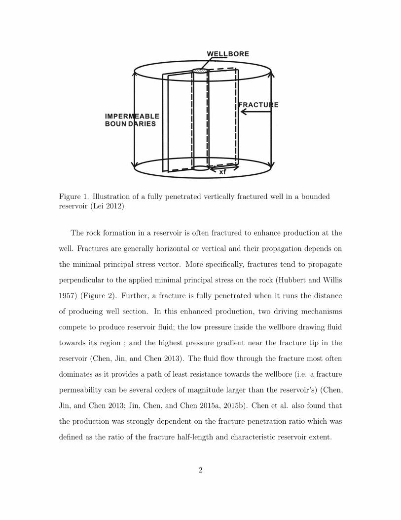
Figure 1. Illustration of a fully penetrated vertically fractured well in a boundedreservoir (Lei 2012)
The rock formation in a reservoir is often fractured to enhance production at the
well. Fractures are generally horizontal or vertical and their propagation depends on
the minimal principal stress vector. More specifically, fractures tend to propagate
perpendicular to the applied minimal principal stress on the rock (Hubbert and Willis
1957) (Figure 2). Further, a fracture is fully penetrated when it runs the distance
of producing well section. In this enhanced production, two driving mechanisms
compete to produce reservoir fluid; the low pressure inside the wellbore drawing fluid
towards its region ; and the highest pressure gradient near the fracture tip in the
reservoir (Chen, Jin, and Chen 2013). The fluid flow through the fracture most often
dominates as it provides a path of least resistance towards the wellbore (i.e. a fracture
permeability can be several orders of magnitude larger than the reservoir’s) (Chen,
Jin, and Chen 2013; Jin, Chen, and Chen 2015a, 2015b). Chen et al. also found that
the production was strongly dependent on the fracture penetration ratio which was
defined as the ratio of the fracture half-length and characteristic reservoir extent.
2
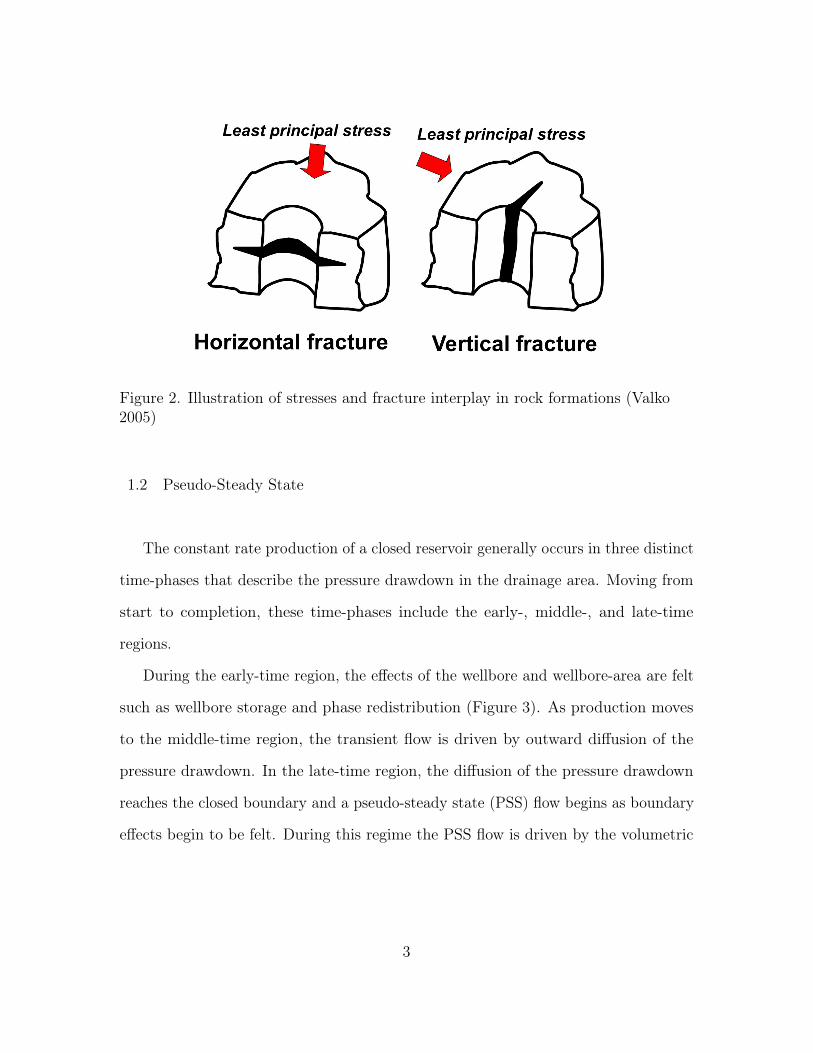
Figure 2. Illustration of stresses and fracture interplay in rock formations (Valko2005)
1.2 Pseudo-Steady State
The constant rate production of a closed reservoir generally occurs in three distinct
time-phases that describe the pressure drawdown in the drainage area. Moving from
start to completion, these time-phases include the early-, middle-, and late-time
regions.
During the early-time region, the effects of the wellbore and wellbore-area are felt
such as wellbore storage and phase redistribution (Figure 3). As production moves
to the middle-time region, the transient flow is driven by outward diffusion of the
pressure drawdown. In the late-time region, the diffusion of the pressure drawdown
reaches the closed boundary and a pseudo-steady state (PSS) flow begins as boundary
effects begin to be felt. During this regime the PSS flow is driven by the volumetric
3
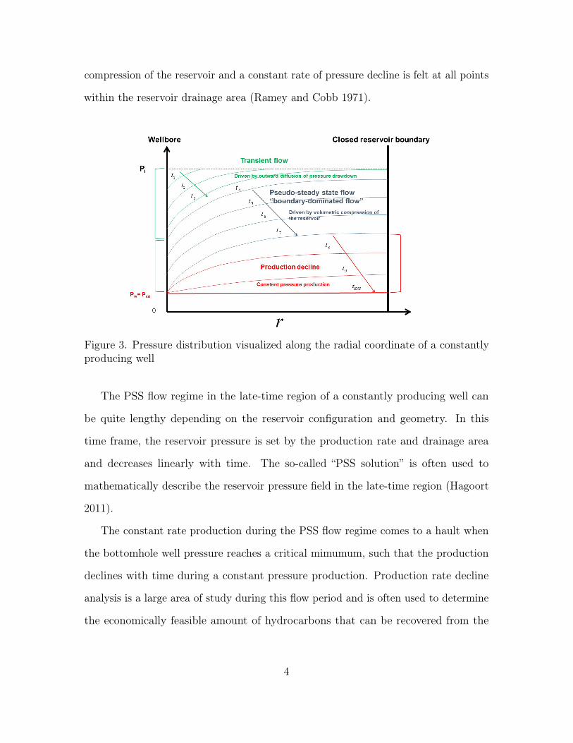
compression of the reservoir and a constant rate of pressure decline is felt at all points
within the reservoir drainage area (Ramey and Cobb 1971).
Figure 3. Pressure distribution visualized along the radial coordinate of a constantlyproducing well
The PSS flow regime in the late-time region of a constantly producing well can
be quite lengthy depending on the reservoir configuration and geometry. In this
time frame, the reservoir pressure is set by the production rate and drainage area
and decreases linearly with time. The so-called “PSS solution” is often used to
mathematically describe the reservoir pressure field in the late-time region (Hagoort
2011).
The constant rate production during the PSS flow regime comes to a hault when
the bottomhole well pressure reaches a critical mimumum, such that the production
declines with time during a constant pressure production. Production rate decline
analysis is a large area of study during this flow period and is often used to determine
the economically feasible amount of hydrocarbons that can be recovered from the
4
reservoir (Arps 1945; Fetkovich et al. 1987; Economides et al. 2013). The PSS solution
is included in various production analyses during this period as it immediately proceeds
the production rate decline period (Doublet and Blasingame 1995; Fetkovich 1980).
More specifically, the dimensionless PSS pressure drawdown at the wellbore is used in
these analyses and is described as
∆pwD,PSS = 2πtDA + bD,PSS (1.1)
where tDA is the dimensionless time based on drainage area, and bD,PSS is the
commonly termed PSS constant. The characteristic drainage-area based time and
characteristic pressure drawdown at the wellbore are nondimensionalized to form these
variables as such,
tDA =κt
µctφA(1.2)
and
∆pwD,PSS =2πκh
µQD
(pi,d − pw,d) (1.3)
where κ is the permeability of the reservoir, h is the formation thickness, µ is the
fluid viscosity, QD is the volumetric production rate of the well, φ is the reservoir
porosity, ct is the total compressibility of the reservoir,pi,d is the initial fluid pressure
in the reservoir, A is the drainage area, and pw,d is the pressure drawdown at the well.
The PSS constant is integral to the PSS solution description as it is used to
scale the dimensionless time and rate of pressure decline within the reservoir and is
dependent on the parameters such as the relative wellbore location, reservoir geometry,
fracture orientation and penetration ratio (Chen 2016). Further, the PSS constant is
5
directly related to the productivity index (PI) of a well and therefore directly related
to the dimensionless PI, JD,PSS by
JD,PSS ≡ 1
bD,PSS. (1.4)
The PI is an extremely important parameter that describes the fluid production per
unit pressure drop of a well and has been shown to play a role in fracture optimization
and production optimization (Jin, Chen, and Chen 2015a, 2015b; Lu and Chen
2016). For these reasons, the PSS constant is an extremely important characteristic
to determine for a producing well.
1.3 Pseudo-Steady State Characterization
For unfractured wells in common reservoir geometries, analytical solutions to the
PSS constant are well defined (Hagoort 2011; Raghavan 1993) and can be generalized
for more geometries with shape factors such as those generated by Dietz (Dietz 1965).
Historically, an exact analytical solution for the PSS flow in a circular fractured
reservoir approximated with an elliptical shape was mathematically derived by Prats
et al. in 1962 (Prats, Hazebroek, and Strickler 1962). More specifically the solution
was obtained for a vertically fractured well with closed boundaries. Prats solution was
however based on an unrealistic assumption of infinite fracture conductivity, hindering
it’s applicability and accuracy (Chen 2016). In 2016, Chen was able to extend the
work of Prats and determine the exact analytical solution to describe the PSS flow
(and therefore the PSS constant) in a fully penetrated vertically fractured well with
finite conductivity and large elliptical shape similar to Figure 4 (ibid).
6
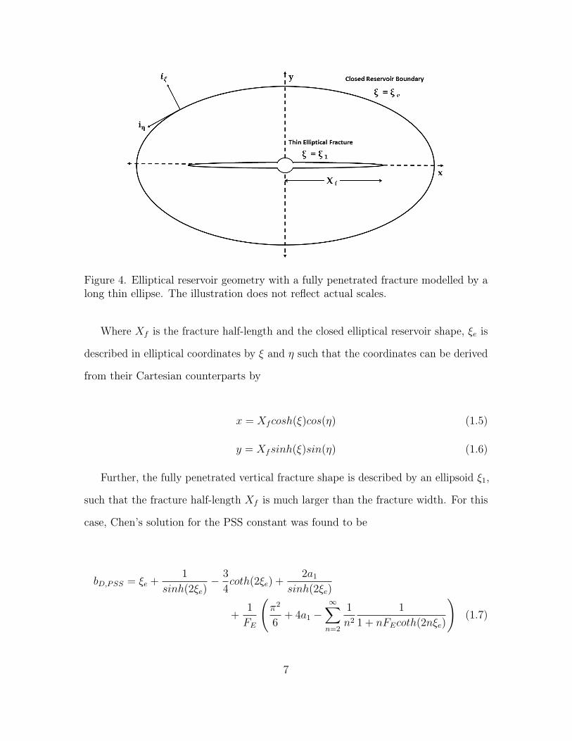
Figure 4. Elliptical reservoir geometry with a fully penetrated fracture modelled by along thin ellipse. The illustration does not reflect actual scales.
Where Xf is the fracture half-length and the closed elliptical reservoir shape, ξe is
described in elliptical coordinates by ξ and η such that the coordinates can be derived
from their Cartesian counterparts by
x = Xfcosh(ξ)cos(η) (1.5)
y = Xfsinh(ξ)sin(η) (1.6)
Further, the fully penetrated vertical fracture shape is described by an ellipsoid ξ1,
such that the fracture half-length Xf is much larger than the fracture width. For this
case, Chen’s solution for the PSS constant was found to be
bD,PSS = ξe +1
sinh(2ξe)− 3
4coth(2ξe) +
2a1sinh(2ξe)
+1
FE
(π2
6+ 4a1 −
∞∑n=2
1
n2
1
1 + nFEcoth(2nξe)
)(1.7)
7
with
a1 = −1
8
1
cosh(2ξe) + sinh(2ξe)FE
(1 +
2
FEsinh(2ξe)
). (1.8)
Where, FE is the dimensionless elliptical fracture conductivity described by
FE =κfwfκXf
(1.9)
and κf is the permeability of the fracture, and wf represents the fracture width.
The solution has also been shown to accurately model circular drainage areas with a
shape-approximation-induced error of less than 1 % for fracture penetration ratios up
to 53 % (Lu and Chen 2016).
Despite this promising new analytical solution for elliptical wells, there are still
gaps in determining an accurate solution for the PSS constant for geometries outside of
elliptical or circular. Several groups have produced approximate solutions for reservoir
geometries including square and rectangular (Lu and Tiab 2010; Goode and Kuchuk
1991; Hagoort 2009; Russell and Truitt 1964; Matthews, Brons, and Hazebroek 1954),
however many of the approximations contained flawed assumptions and bases. The
alternative to determine an accurate PSS constant is through the numerical simulation
of each reservoir of interest, which has been documented as extremely time consuming
and mathematically intensive as the PSS constant can be subtracted from the scaled
drainage area based dimensionless time when the long-time data set of dimensionless
pressure drawdown is found (Blasingame, Amini, and Rushing 2007).
8
1.4 Purpose
The purpose of this research is to determine and execute a suitable general
methodology to generate high fidelity shape factors to modify Chen’s PSS constant
solution for fully penetrated vertically fractured wells in a closed elliptical reservoir.
More specifically shape factors to modify the exact PSS solution for rectangular,
triangular, and rhomboid closed reservoir geometries with concentric fully penetrated
vertically fractured wells are considered.
9
Chapter 2
METHODOLOGY
2.1 Overview
The general procedure to create shape factors that augment Chen’s solution was to
determine the true PSS constant for various reservoir geometries and then compare it
to a PSS constant approximation from the elliptical reservoir analytical solution based
on an assumed equivalence point. Then, by ratioing the true and predicted solution
over several case studies of a geometry, trends could be observed and characterized in
order to create a shape factor that modulates Chen’s solution accordingly to accurately
describe the true PSS constant.
2.2 COMSOL Multiphysics Modeling
Consider a fully penetrated vertically fractured well centrally located in a closed
reservoir of generic shape. The well is producing at a constant rate and a sufficient
period of time has passed such that outer-boundary effects are being felt and the fluid
is described by PSS flow. The flowing reservoir fluid is assumed to be single-phase in
a homogeneous formation, where the fluid and reservoir are weakly compressible and
can thus be described by a single lumped compressibility constant. The fracture is
assumed to be supported by proppants and is considered incompressible. Moreover,
the permeability of the fracture is taken to be much larger than the formation inferring
that all production is from the fracture. The fracture is width is also defined to be
10
much smaller than the length of the fracture as well as the diameter of the wellbore.
The fluid motion in the finite formation and fracture is governed by Darcy’s law, and
any effects of wellbore storage and skin are negligible.
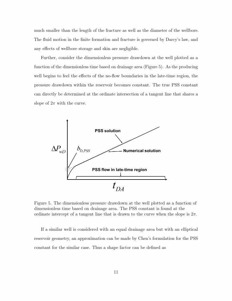
Further, consider the dimensionless pressure drawdown at the well plotted as a
function of the dimensionless time based on drainage area (Figure 5). As the producing
well begins to feel the effects of the no-flow boundaries in the late-time region, the
pressure drawdown within the reservoir becomes constant. The true PSS constant
can directly be determined at the ordinate intersection of a tangent line that shares a
slope of 2π with the curve.
Figure 5. The dimensionless pressure drawdown at the well plotted as a function ofdimensionless time based on drainage area. The PSS constant is found at theordinate intercept of a tangent line that is drawn to the curve when the slope is 2π.
If a similar well is considered with an equal drainage area but with an elliptical
reservoir geometry, an approximation can be made by Chen’s formulation for the PSS
constant for the similar case. Thus a shape factor can be defined as
11
Ca,f ≡bD,PSSbD,PSSA
(2.1)
where bD,PSS is the true PSS constant of the case study and bD,PSSA is the
approximated PSS constant using the exact analytical solution for reservoirs of
elliptical shape. Thus a shape factor for a particular well geometry and configuration
is made which corrects the approximation to the true value. If several case studies
with variable penetration ratios are completed for a certain geometry, the shape factor
can be applied to a larger set of reservoir configurations through interpolations and
curve fitting.
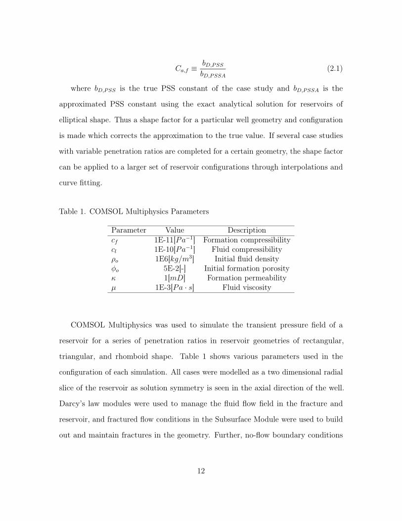
Table 1. COMSOL Multiphysics Parameters
Parameter Value Descriptioncf 1E-11[Pa−1] Formation compressibilitycl 1E-10[Pa−1] Fluid compressibilityρo 1E6[kg/m3] Initial fluid densityφo 5E-2[-] Initial formation porosityκ 1[mD] Formation permeabilityµ 1E-3[Pa · s] Fluid viscosity
COMSOL Multiphysics was used to simulate the transient pressure field of a
reservoir for a series of penetration ratios in reservoir geometries of rectangular,
triangular, and rhomboid shape. Table 1 shows various parameters used in the
configuration of each simulation. All cases were modelled as a two dimensional radial
slice of the reservoir as solution symmetry is seen in the axial direction of the well.
Darcy’s law modules were used to manage the fluid flow field in the fracture and
reservoir, and fractured flow conditions in the Subsurface Module were used to build
out and maintain fractures in the geometry. Further, no-flow boundary conditions
12
were made at the reservoir boundaries to simulate a closed finite formation. The well
was located centrally across all case studies in the present work for simplicity. Along
with the aforementioned assumptions, the following parameters were also used in all
case studies to define the well configuration and case study. The penetration ratio for
each case study was varied by maintaining a constant characteristic boundary length
while modulating the fracture half-length.
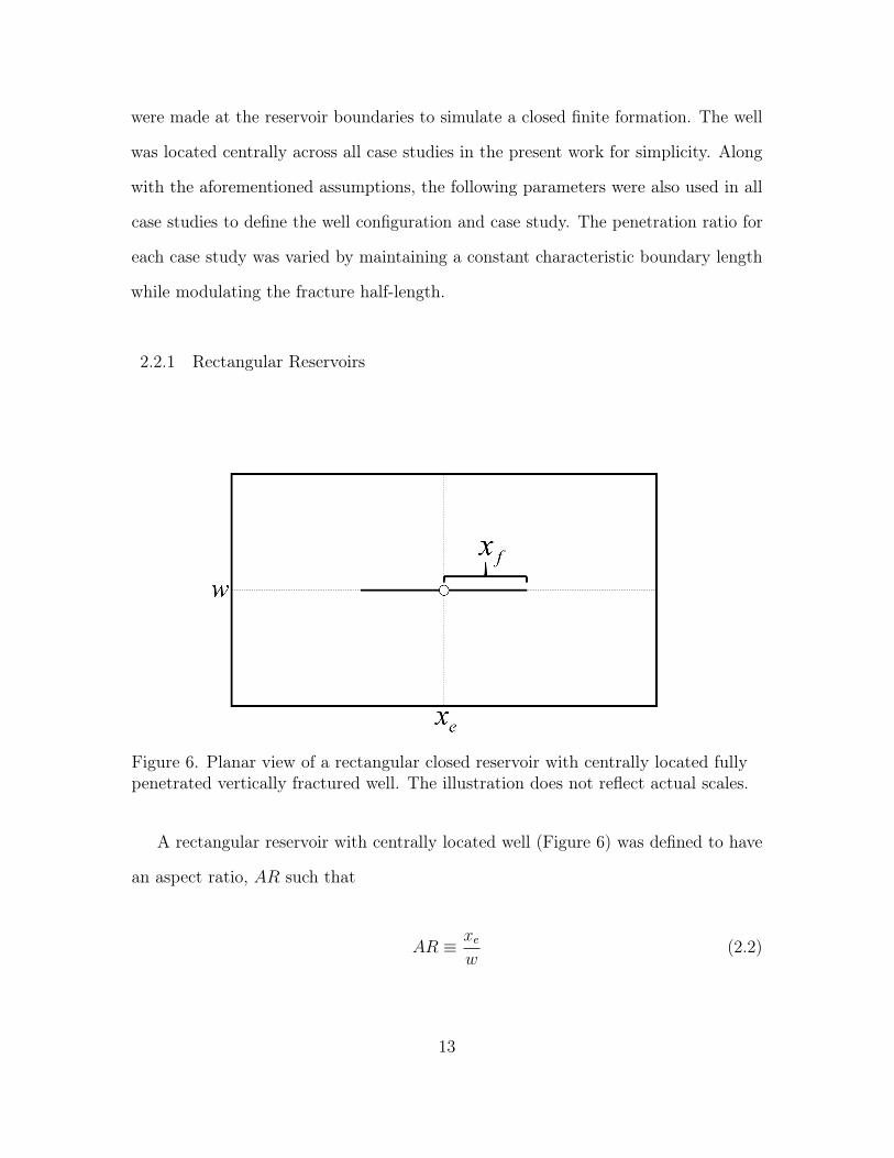
2.2.1 Rectangular Reservoirs
Figure 6. Planar view of a rectangular closed reservoir with centrally located fullypenetrated vertically fractured well. The illustration does not reflect actual scales.
A rectangular reservoir with centrally located well (Figure 6) was defined to have
an aspect ratio, AR such that
AR ≡ xew
(2.2)
13
where xe was the reservoir characteristic side length (reservoir drainage extent)
and w was the reservoir width. The rectangular penetration ratio was defined as
Ix =2xfxe
(2.3)
where xf was the fracture half-length. Rectangular geometries of aspect ratio 1
(square), 2, 3, and 4 were studied at various penetration ratios up to 50% as ratios
above this are rarely seen in-field.
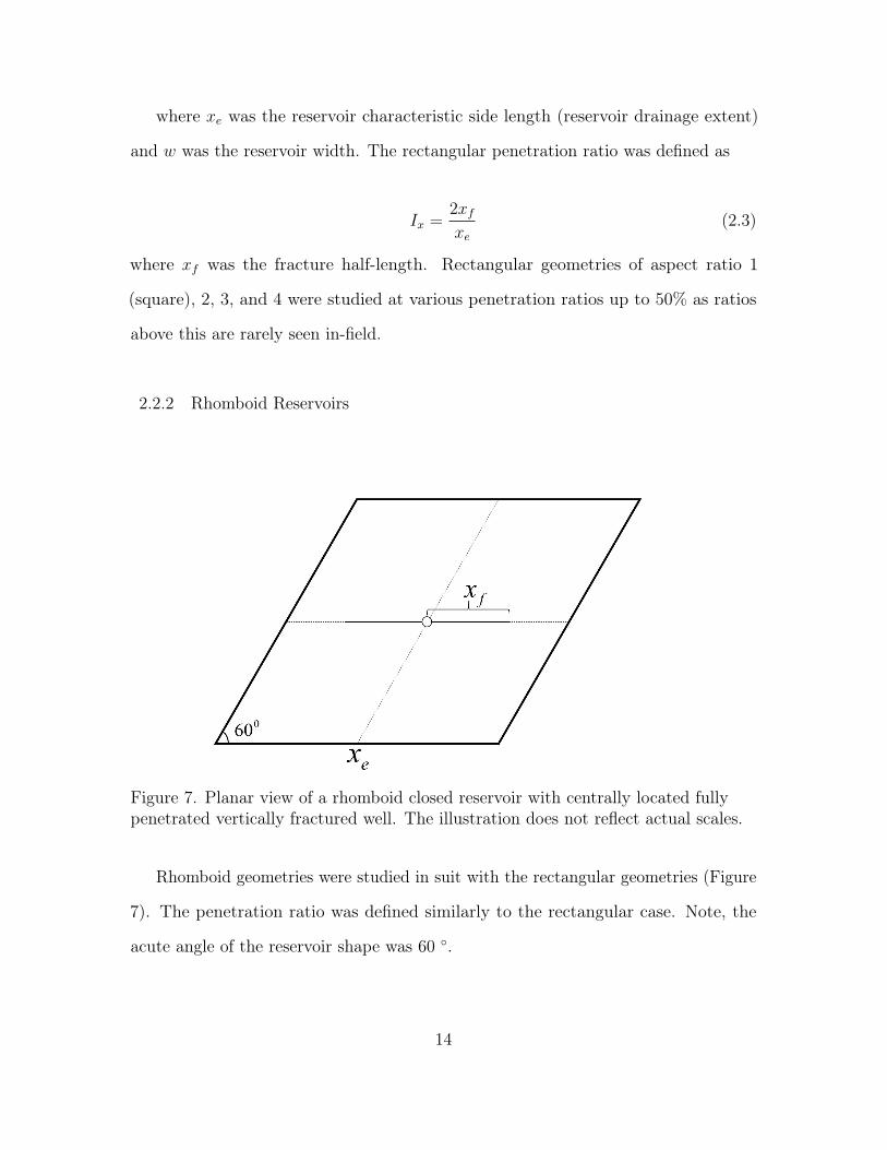
2.2.2 Rhomboid Reservoirs
Figure 7. Planar view of a rhomboid closed reservoir with centrally located fullypenetrated vertically fractured well. The illustration does not reflect actual scales.
Rhomboid geometries were studied in suit with the rectangular geometries (Figure
7). The penetration ratio was defined similarly to the rectangular case. Note, the
acute angle of the reservoir shape was 60 ◦.
14
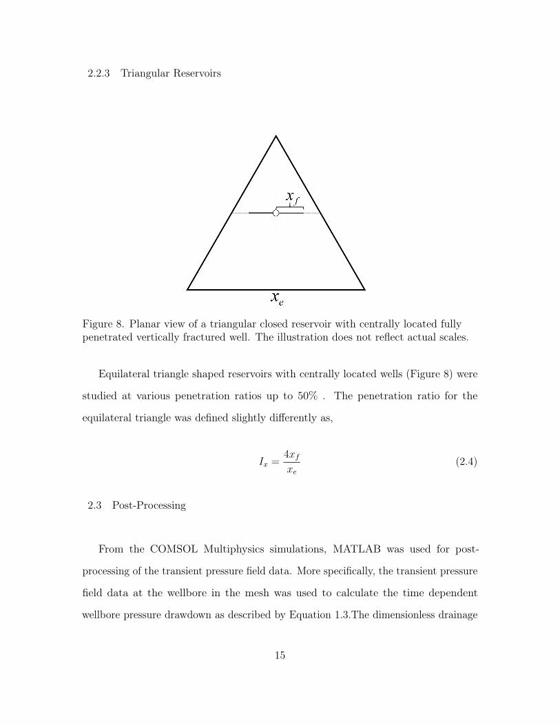
2.2.3 Triangular Reservoirs
Figure 8. Planar view of a triangular closed reservoir with centrally located fullypenetrated vertically fractured well. The illustration does not reflect actual scales.
Equilateral triangle shaped reservoirs with centrally located wells (Figure 8) were
studied at various penetration ratios up to 50% . The penetration ratio for the
equilateral triangle was defined slightly differently as,
Ix =4xfxe
(2.4)
2.3 Post-Processing
From the COMSOL Multiphysics simulations, MATLAB was used for post-
processing of the transient pressure field data. More specifically, the transient pressure
field data at the wellbore in the mesh was used to calculate the time dependent
wellbore pressure drawdown as described by Equation 1.3.The dimensionless drainage
15
area based time was calculated by Equation 1.2. The true PSS constant could then
be determined as previously described and compared to an approximation of the PSS
constant by Chen’s solution assuming an equal drainage area.
Once the shape factors were determined, two parameter one-variable curve fitting
via non-linear regression was conducted by fitting curve shapes to over 200 non-linear
functions in Lab Fit to determine the form with the least residual error and root mean
squared error.
16
Chapter 3
RESULTS
3.1 Rectangular Shape Factor
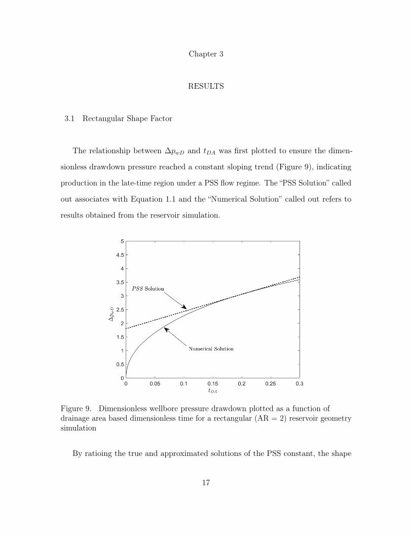
The relationship between ∆pwD and tDA was first plotted to ensure the dimen-
sionless drawdown pressure reached a constant sloping trend (Figure 9), indicating
production in the late-time region under a PSS flow regime. The “PSS Solution” called
out associates with Equation 1.1 and the “Numerical Solution” called out refers to
results obtained from the reservoir simulation.
Figure 9. Dimensionless wellbore pressure drawdown plotted as a function ofdrainage area based dimensionless time for a rectangular (AR = 2) reservoir geometrysimulation
By ratioing the true and approximated solutions of the PSS constant, the shape
17
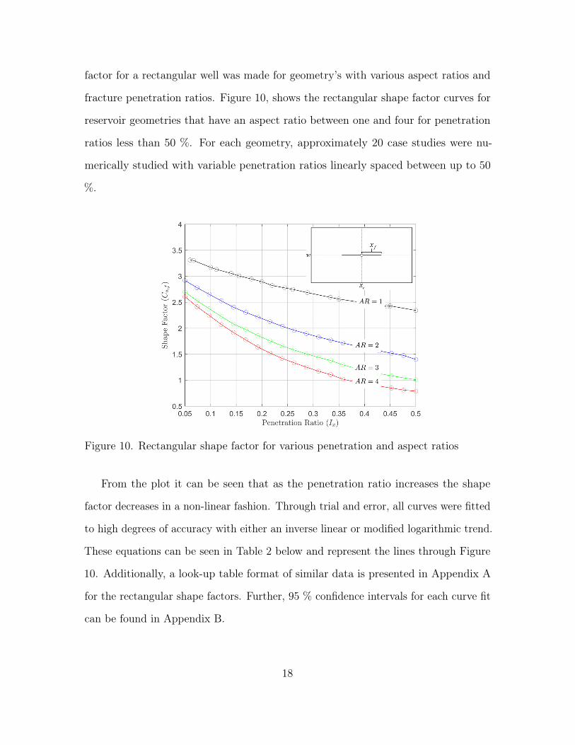
factor for a rectangular well was made for geometry’s with various aspect ratios and
fracture penetration ratios. Figure 10, shows the rectangular shape factor curves for
reservoir geometries that have an aspect ratio between one and four for penetration
ratios less than 50 %. For each geometry, approximately 20 case studies were nu-
merically studied with variable penetration ratios linearly spaced between up to 50
%.
Figure 10. Rectangular shape factor for various penetration and aspect ratios
From the plot it can be seen that as the penetration ratio increases the shape
factor decreases in a non-linear fashion. Through trial and error, all curves were fitted
to high degrees of accuracy with either an inverse linear or modified logarithmic trend.
These equations can be seen in Table 2 below and represent the lines through Figure
10. Additionally, a look-up table format of similar data is presented in Appendix A
for the rectangular shape factors. Further, 95 % confidence intervals for each curve fit
can be found in Appendix B.
18
3.2 Rhomboid Shape Factor
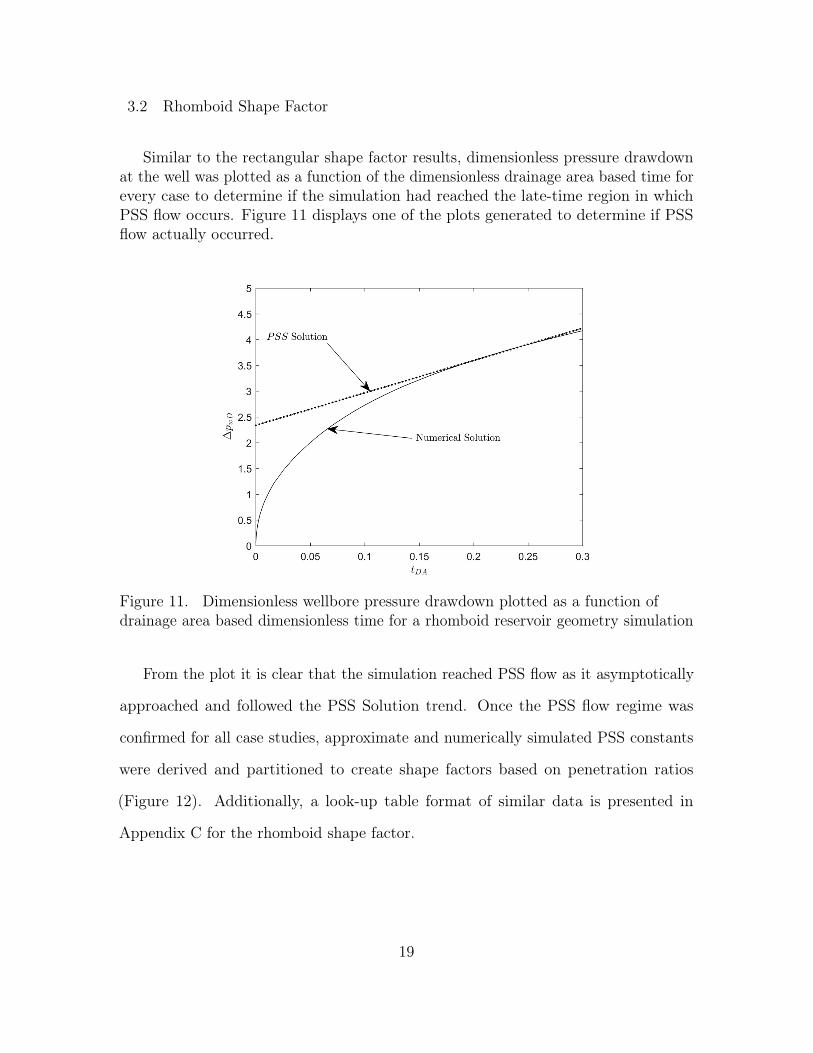
Similar to the rectangular shape factor results, dimensionless pressure drawdownat the well was plotted as a function of the dimensionless drainage area based time forevery case to determine if the simulation had reached the late-time region in whichPSS flow occurs. Figure 11 displays one of the plots generated to determine if PSSflow actually occurred.
Figure 11. Dimensionless wellbore pressure drawdown plotted as a function ofdrainage area based dimensionless time for a rhomboid reservoir geometry simulation
From the plot it is clear that the simulation reached PSS flow as it asymptotically
approached and followed the PSS Solution trend. Once the PSS flow regime was
confirmed for all case studies, approximate and numerically simulated PSS constants
were derived and partitioned to create shape factors based on penetration ratios
(Figure 12). Additionally, a look-up table format of similar data is presented in
Appendix C for the rhomboid shape factor.
19
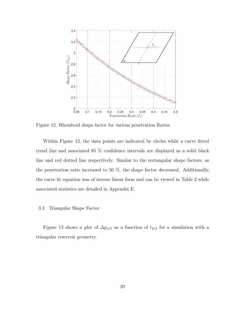
Figure 12. Rhomboid shape factor for various penetration Ratios
Within Figure 12, the data points are indicated by circles while a curve fitted
trend line and associated 95 % confidence intervals are displayed as a solid black
line and red dotted line respectively. Similar to the rectangular shape factors, as
the penetration ratio increased to 50 %, the shape factor decreased. Additionally,
the curve fit equation was of inverse linear form and can be viewed in Table 2 while
associated statistics are detailed in Appendix E.
3.3 Triangular Shape Factor
Figure 13 shows a plot of ∆pwD as a function of tDA for a simulation with a
triangular reservoir geometry.
20
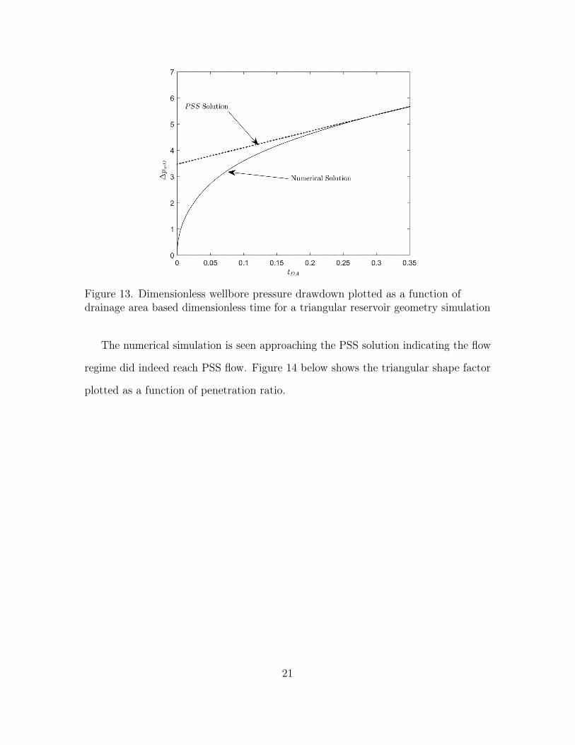
Figure 13. Dimensionless wellbore pressure drawdown plotted as a function ofdrainage area based dimensionless time for a triangular reservoir geometry simulation
The numerical simulation is seen approaching the PSS solution indicating the flow
regime did indeed reach PSS flow. Figure 14 below shows the triangular shape factor
plotted as a function of penetration ratio.
21
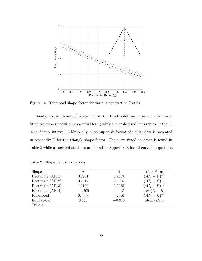
Figure 14. Rhomboid shape factor for various penetration Ratios
Similar to the rhomboid shape factor, the black solid line represents the curve
fitted equation (modified exponential form) while the dashed red lines represent the 95
% confidence interval. Additionally, a look-up table format of similar data is presented
in Appendix D for the triangle shape factor. The curve fitted equation is found in
Table 2 while associated statistics are found in Appendix E for all curve fit equations.
Table 2. Shape Factor Equations
Shape A B Ca,f FormRectangle (AR 1) 0.2931 0.2863 (AIx +B)−1
Rectangle (AR 2) 0.7914 0.3015 (AIx +B)−1
Rectangle (AR 3) 1.3130 0.2965 (AIx +B)−1
Rectangle (AR 4) −1.205 0.0618 Aln(Ix +B)Rhomboid 0.3698 0.2906 (AIx +B)−1
EquilateralTriangle
3.060 −0.970 Aexp(BIx)
22
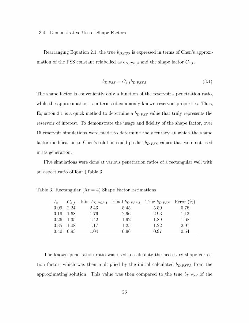
3.4 Demonstrative Use of Shape Factors
Rearranging Equation 2.1, the true bD,PSS is expressed in terms of Chen’s approxi-
mation of the PSS constant relabelled as bD,PSSA and the shape factor Ca,f .
bD,PSS = Ca,fbD,PSSA (3.1)
The shape factor is conveniently only a function of the reservoir’s penetration ratio,
while the approximation is in terms of commonly known reservoir properties. Thus,
Equation 3.1 is a quick method to determine a bD,PSS value that truly represents the
reservoir of interest. To demonstrate the usage and fidelity of the shape factor, over
15 reservoir simulations were made to determine the accuracy at which the shape
factor modification to Chen’s solution could predict bD,PSS values that were not used
in its generation.
Five simulations were done at various penetration ratios of a rectangular well with
an aspect ratio of four (Table 3.
Table 3. Rectangular (Ar = 4) Shape Factor Estimations
Ix Ca,f Init. bD,PSSA Final bD,PSSA True bD,PSS Error (%)0.09 2.24 2.43 5.45 5.50 0.760.19 1.68 1.76 2.96 2.93 1.130.26 1.35 1.42 1.92 1.89 1.680.35 1.08 1.17 1.25 1.22 2.970.40 0.93 1.04 0.96 0.97 0.54
The known penetration ratio was used to calculate the necessary shape correc-
tion factor, which was then multiplied by the initial calculated bD,PSSA from the
approximating solution. This value was then compared to the true bD,PSS of the
23
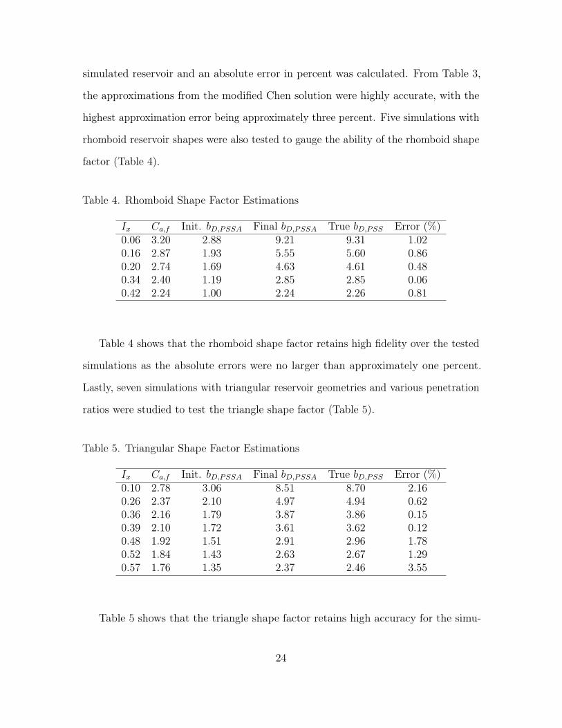
simulated reservoir and an absolute error in percent was calculated. From Table 3,
the approximations from the modified Chen solution were highly accurate, with the
highest approximation error being approximately three percent. Five simulations with
rhomboid reservoir shapes were also tested to gauge the ability of the rhomboid shape
factor (Table 4).
Table 4. Rhomboid Shape Factor Estimations
Ix Ca,f Init. bD,PSSA Final bD,PSSA True bD,PSS Error (%)0.06 3.20 2.88 9.21 9.31 1.020.16 2.87 1.93 5.55 5.60 0.860.20 2.74 1.69 4.63 4.61 0.480.34 2.40 1.19 2.85 2.85 0.060.42 2.24 1.00 2.24 2.26 0.81
Table 4 shows that the rhomboid shape factor retains high fidelity over the tested
simulations as the absolute errors were no larger than approximately one percent.
Lastly, seven simulations with triangular reservoir geometries and various penetration
ratios were studied to test the triangle shape factor (Table 5).
Table 5. Triangular Shape Factor Estimations
Ix Ca,f Init. bD,PSSA Final bD,PSSA True bD,PSS Error (%)0.10 2.78 3.06 8.51 8.70 2.160.26 2.37 2.10 4.97 4.94 0.620.36 2.16 1.79 3.87 3.86 0.150.39 2.10 1.72 3.61 3.62 0.120.48 1.92 1.51 2.91 2.96 1.780.52 1.84 1.43 2.63 2.67 1.290.57 1.76 1.35 2.37 2.46 3.55
Table 5 shows that the triangle shape factor retains high accuracy for the simu-
24

lations studied. It is worthy to note that two scenarios were tested over the 50 %
penetration ratio cap, and high accuracy was still achieved, as the error remained
under five percent.
25
Chapter 4
DISCUSSION
Shape factors for concentrically placed wells in rectangular, rhomboid, and tri-
angular reservoir geometries were successfully derived for penetration ratios below
50 % which are ratios most commonly seen in-field. Further, all shape factor curves
were characterized using non-linear regression. All regression models were in terms
of inverse linear, modified exponential, or modified logarithm functions with I[x] as
a sole variable and two regression coefficients. The culminating results of the work
were presented in Figures 10,12, and 14 which graphically displayed the various shape
factors and Table 2 which compiled all the curve fitted equations that characterize
the generated shape factor curves.
Nearly 80 various well configurations were simulated in rectangular reservoirs to
generate shape factors for rectangular reservoir drainage areas with aspect ratios
ranging between one and four. Further, 20 various well configurations were simulated
for both rhomboid and triangular reservoir shapes to generate shape factors. Due to
all the shape factor data generally following smooth trends, curve fitting was found
to be quite successful at describing the data sets. This was visualized with tight
95% confidence intervals and backed by further statistics seen in Appendix E. For
example, the mean absolute percentage error for out of sample validation was found
to be 1.41 % , 1.38 %, and 0.65 % for the rectangular, triangular, and rhomboid shape
factors respectfully. Further the root mean squared error for all curve fits were under
0.02, indicating that the regressor coefficients and accompanying form for each fit was
predicting data with high accuracy.
26
For the rectangular shape factors, as the aspect ratio increased, the shape factor
curve translated lower. A lower shape factor indicates that the unmodified approxima-
tion was closer to the true PSS value when compared to higher shape factor numbers.
In speculation, reservoirs with larger aspect ratios may be more geometrically similar
to the ellipsoid, ξe that is approximating it when compared to reservoirs with smaller
aspect ratios. Additionally, for all shape factors, as the Ix increased to 50 % the shape
factor decreased in a non-linear fashion. In conjecture, this could be because the large
penetration ratios indicate larger fractures which may be more geometrically similar
to the penetration ratio definition for elliptical wells.
27
Chapter 5
CONCLUSIONS
The PSS constant is an important parameter that is used to describe the PSS
dimensionless pressure drawdown at the well in a reservoir during the late-time region
of fluid production. The PSS also directly relates to the dimensionless PI of a well
which has been shown to be important during fracture optimization and production
rate decline analysis.
In 2016, Chen mathematically derived the exact analytical solution to describe the
PSS constant in a fully penetrated vertically fractured well in an elliptical reservoir. By
using extensive computational modeling, the current work extends Chen’s solution by
introducing shape factors to widen the applicability to wells of rectangular, rhomboid,
and triangular reservoir geometries. More specifically, shape factors were made
for concentric wells in rectangular geometries of AR 1-4, equilateral triangles, and
rhomboids. The shape factors were made a function of the penetration ratio and
are applicable under Ix 6 50%. Further, characterization using curve fitting was
conducted for quick spreadsheet calculations while look-up tables were generated for
in-field use. Example usage of the shape factors was conducted and demonstrated
the high fidelity of the shape factors to reproduce accurate PSS constant predictions.
Across all shape factors, the mean absolute error in validation case studies were under
1.5 % using the curve fitted equations that were generated in Table 2.
28
5.1 Future Work
This work has laid the foundation methodology to create additional shape factors
to describe various well configurations not studied presently. In the immediate future,
shape factors for parallelograms with various aspect ratios and reservoirs with non-
concentric wells should be studied to build out the coverage of shape factors to
modulate Chen’s solution. Lastly, the effects of fracture orientation within these
geometries would provide a more complete package for the shape factors to be used.
29
REFERENCES
Arps, J.J. 1945. “Analysis of Decline Curves.” Transactions of the AIME 160, no. 01(): 228–247. doi:10.2118/945228-G.
Beaumont Norman H., Edward A Foster, ed. 1999. Exploring for Oil and Gas Traps.American Association of Petroleum Geologists. http://geoscienceworld.org/content/9781629810744/9781629810744.
Blasingame, Thomas Alwin, Shahram Amini, and Jay Rushing. 2007. “Evaluationof the Elliptical Flow Period for Hydraulically-Fractured Wells in Tight GasSands – Theoretical Aspects and Practical Considerations.” In SPE HydraulicFracturing Technology Conference. College Station, Texas, U.S.A: Society ofPetroleum Engineers. doi:10.2118/106308-MS.
Chen, Kang Ping. 2016. “Production From a Fractured Well With Finite Fracture Con-ductivity in a Closed Reservoir: An Exact Analytical Solution for Pseudosteady-State Flow.” SPE Journal 21, no. 02 (): 550–556. doi:10.2118/179739-PA.
Chen, Kang Ping, Yan Jin, and Mian Chen. 2013. “Pressure-gradient singularity andproduction enhancement for hydraulically fractured wells.” Geophysical JournalInternational 195, no. 2 (): 923–931. doi:10.1093/gji/ggt272.
Dietz, D.N. 1965. “Determination of Average Reservoir Pressure From Build-UpSurveys.” Journal of Petroleum Technology 17, no. 08 (): 955–959. doi:10.2118/1156-PA.
Doublet, L.E., and T.A. Blasingame. 1995. “Decline Curve Analysis Using Type Curves:Water Influx/Waterflood Cases.” In 1995 Annual SPE Technical Conference andExhibition. Dallas, TX, USA: Society of Petroleum Engineers.
Economides, Michael J., Daniel A. Hill, Christine Ehlig-Economides, and Ding Zhu.2013. Petroleum production systems. 2nd ed. Upper Saddle River: Prentice Hall.
Fetkovich, M J, M E Vienot, M D Bradley, and U G Kiesow. 1987. “Decline CurveAnalysis Using Type Curves: Case Histories.” SPE Formation Evaluation 2 (4):637–656. doi:10.2118/13169-PA.
Fetkovich, M.J. 1980. “Decline Curve Analysis Using Type Curves.” Journal ofPetroleum Technology 32, no. 06 (): 1065–1077. doi:10.2118/4629-PA.
Goode, P.A., and F.J. Kuchuk. 1991. “Inflow Performance of Horizontal Wells.” SPEReservoir Engineering 6, no. 03 (): 319–323. doi:10.2118/21460-PA.
30

Hagoort, Jacques. 2009. “The Productivity of a Well with a Vertical Infinite-Conductivity Fracture in a Rectangular Closed Reservoir.” SPE Journal 14,no. 04 (): 715–720. doi:10.2118/112975-PA.
. 2011. “Semisteady-State Productivity of a Well in a Rectangular ReservoirProducing at Constant Rate or Constant Pressure.” SPE Reservoir Evaluation &Engineering 14, no. 06 (): 677–686. doi:10.2118/149807-PA.
Hubbert, M K, and D G Willis. 1957. “Mechanics of Hydraulic Fracturing.” Trans-actions of the AIME (420 Commonwealth Dr, Warrendale, PA 15086) 210 (6):153–163.
Jin, Yan, Kang Ping Chen, and Mian Chen. 2015a. “An asymptotic solution forfluid production from an elliptical hydraulic fracture at early-times.” MechanicsResearch Communications 63 (): 48–53. doi:10.1016/j.mechrescom.2014.12.004.
. 2015b. “Analytical solution and mechanisms of fluid production from hydrauli-cally fractured wells with finite fracture conductivity.” Journal of EngineeringMathematics 92, no. 1 (): 103–122. doi:10.1007/s10665-014-9754-x.
Lu, Jing, and Djebbar Tiab. 2010. “Pseudo-Steady-State Productivity Formula for aPartially Penetrating Vertical Well in a Box-Shaped Reservoir.” MathematicalProblems in Engineering 2010:1–35. doi:10.1155/2010/907206.
Lu, Yunhu, and Kang Ping Chen. 2016. “Productivity-Index Optimization for Hydrauli-cally Fractured Vertical Wells in a Circular Reservoir: A Comparative Study WithAnalytical Solutions.” SPE Journal 21, no. 06 (): 2208–2219. doi:10.2118/180929-PA.
Matthews, C S, F Brons, and P Hazebroek. 1954. “A Method for Determination of Aver-age Pressure in a Bounded Reservoir.” TRANSACTIONS OF THE AMERICANINSTITUTE OF MINING AND METALLURGICAL ENGINEERS 201:182–191.doi:XR348. arXiv: XR348.
Prats, M, P Hazebroek, and W.R. Strickler. 1962. “Effect of Vertical Fractures onReservoir Behavior–Compressible-Fluid Case.” Society of Petroleum EngineersJournal 2, no. 02 (): 87–94. doi:10.2118/98-PA.
Raghavan, R. 1993. Well Test Analysis [in English]. Englewood Cliffs, N.J.: PTRPrentice Hall.
31
Ramey, H.J., and William M Cobb. 1971. “A General Pressure Buildup Theory for aWell in a Closed Drainage Area.” Journal of Petroleum Technology 23, no. 12 ():1493–1505. doi:10.2118/3012-PA.
Russell, D.G., and N.E. Truitt. 1964. “Transient Pressure Behavior in VerticallyFractured Reservoirs.” Journal of Petroleum Technology 16, no. 10 (): 1159–1170.doi:10.2118/967-PA.
Sadeghi, Mohammad, Seyed Reza Shadizadeh, and Mohammad Ali Ahmadi. 2013.“Determination of Drainage Area and Shape Factor of Vertical Wells in Natu-rally Fracture Reservoir with Help Well testing and Developed IPR Curve.” InNorth Africa Technical Conference and Exhibition, vol. 1. April 2013. Society ofPetroleum Engineers. doi:10.2118/164638-MS.
32

APPENDIX A
RECTANGULAR LOOK-UP TABLES
33

Table 6. Rectangular (AR = 1) Shape Factor Look-Up TableIx(%) Ca,f Ix(%) Ca,f0.05 2.92 0.28 2.330.06 2.89 0.29 2.310.07 2.86 0.30 2.290.08 2.84 0.31 2.270.09 2.81 0.32 2.250.10 2.79 0.33 2.230.11 2.76 0.33 2.210.11 2.74 0.34 2.190.12 2.71 0.35 2.170.13 2.69 0.36 2.150.14 2.67 0.37 2.130.15 2.64 0.38 2.120.16 2.62 0.39 2.100.17 2.60 0.40 2.080.18 2.57 0.41 2.060.19 2.55 0.42 2.040.20 2.53 0.43 2.020.21 2.51 0.44 2.010.22 2.48 0.44 1.990.22 2.46 0.45 1.970.23 2.44 0.46 1.950.24 2.42 0.47 1.940.25 2.40 0.48 1.920.26 2.38 0.49 1.900.27 2.35 0.50 1.88
34

Table 7. Rectangular (AR = 2) Shape Factor Look-Up TableIx(%) Ca,f Ix(%) Ca,f0.05 2.92 0.28 2.330.06 2.89 0.29 2.310.07 2.86 0.30 2.290.08 2.84 0.31 2.270.09 2.81 0.32 2.250.10 2.79 0.33 2.230.11 2.76 0.33 2.210.11 2.74 0.34 2.190.12 2.71 0.35 2.170.13 2.69 0.36 2.150.14 2.67 0.37 2.130.15 2.64 0.38 2.120.16 2.62 0.39 2.100.17 2.60 0.40 2.080.18 2.57 0.41 2.060.19 2.55 0.42 2.040.20 2.53 0.43 2.020.21 2.51 0.44 2.010.22 2.48 0.44 1.990.22 2.46 0.45 1.970.23 2.44 0.46 1.950.24 2.42 0.47 1.940.25 2.40 0.48 1.920.26 2.38 0.49 1.900.27 2.35 0.50 1.88
35
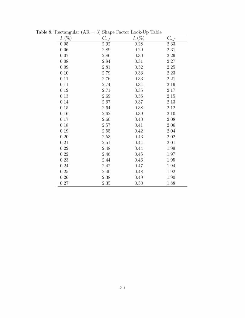
Table 8. Rectangular (AR = 3) Shape Factor Look-Up TableIx(%) Ca,f Ix(%) Ca,f0.05 2.92 0.28 2.330.06 2.89 0.29 2.310.07 2.86 0.30 2.290.08 2.84 0.31 2.270.09 2.81 0.32 2.250.10 2.79 0.33 2.230.11 2.76 0.33 2.210.11 2.74 0.34 2.190.12 2.71 0.35 2.170.13 2.69 0.36 2.150.14 2.67 0.37 2.130.15 2.64 0.38 2.120.16 2.62 0.39 2.100.17 2.60 0.40 2.080.18 2.57 0.41 2.060.19 2.55 0.42 2.040.20 2.53 0.43 2.020.21 2.51 0.44 2.010.22 2.48 0.44 1.990.22 2.46 0.45 1.970.23 2.44 0.46 1.950.24 2.42 0.47 1.940.25 2.40 0.48 1.920.26 2.38 0.49 1.900.27 2.35 0.50 1.88
36

Table 9. Rectangular (AR = 4) Shape Factor Look-Up TableIx(%) Ca,f Ix(%) Ca,f0.05 2.92 0.28 2.330.06 2.89 0.29 2.310.07 2.86 0.30 2.290.08 2.84 0.31 2.270.09 2.81 0.32 2.250.10 2.79 0.33 2.230.11 2.76 0.33 2.210.11 2.74 0.34 2.190.12 2.71 0.35 2.170.13 2.69 0.36 2.150.14 2.67 0.37 2.130.15 2.64 0.38 2.120.16 2.62 0.39 2.100.17 2.60 0.40 2.080.18 2.57 0.41 2.060.19 2.55 0.42 2.040.20 2.53 0.43 2.020.21 2.51 0.44 2.010.22 2.48 0.44 1.990.22 2.46 0.45 1.970.23 2.44 0.46 1.950.24 2.42 0.47 1.940.25 2.40 0.48 1.920.26 2.38 0.49 1.900.27 2.35 0.50 1.88
37

APPENDIX B
RECTANGULAR SHAPE FACTOR CONFIDENCE INTERVALS
38
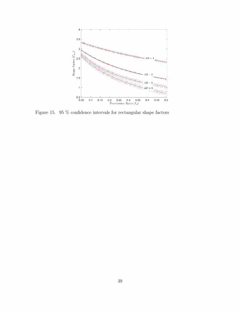
Figure 15. 95 % confidence intervals for rectangular shape factors
39

APPENDIX C
RHOMBOID LOOK-UP TABLE
40
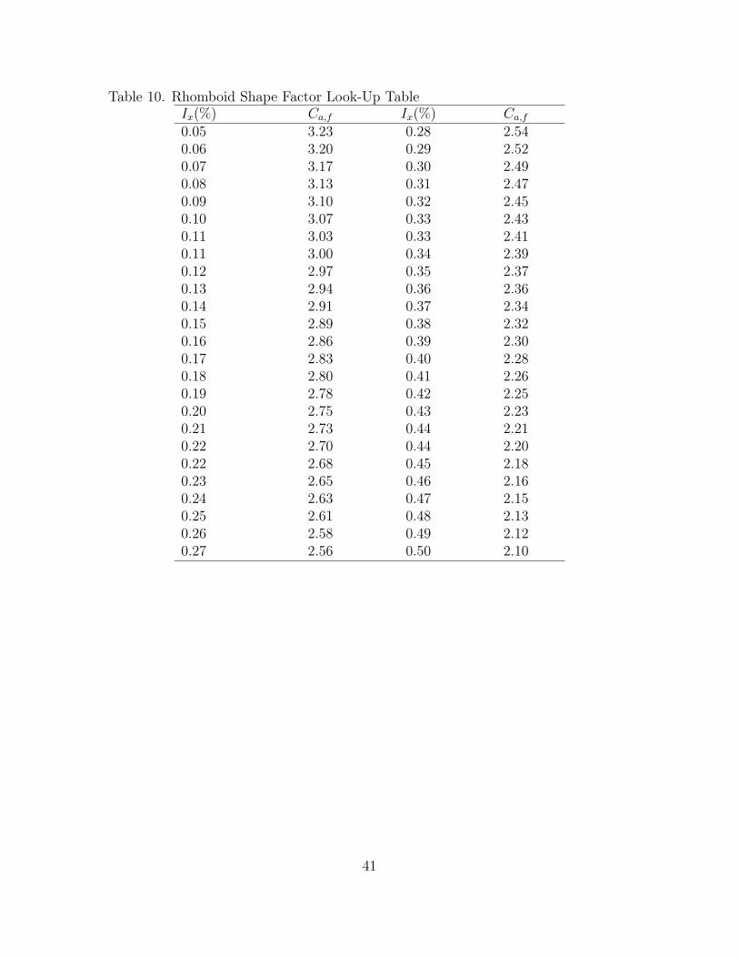
Table 10. Rhomboid Shape Factor Look-Up TableIx(%) Ca,f Ix(%) Ca,f0.05 3.23 0.28 2.540.06 3.20 0.29 2.520.07 3.17 0.30 2.490.08 3.13 0.31 2.470.09 3.10 0.32 2.450.10 3.07 0.33 2.430.11 3.03 0.33 2.410.11 3.00 0.34 2.390.12 2.97 0.35 2.370.13 2.94 0.36 2.360.14 2.91 0.37 2.340.15 2.89 0.38 2.320.16 2.86 0.39 2.300.17 2.83 0.40 2.280.18 2.80 0.41 2.260.19 2.78 0.42 2.250.20 2.75 0.43 2.230.21 2.73 0.44 2.210.22 2.70 0.44 2.200.22 2.68 0.45 2.180.23 2.65 0.46 2.160.24 2.63 0.47 2.150.25 2.61 0.48 2.130.26 2.58 0.49 2.120.27 2.56 0.50 2.10
41

APPENDIX D
TRIANGULAR LOOK-UP TABLE
42
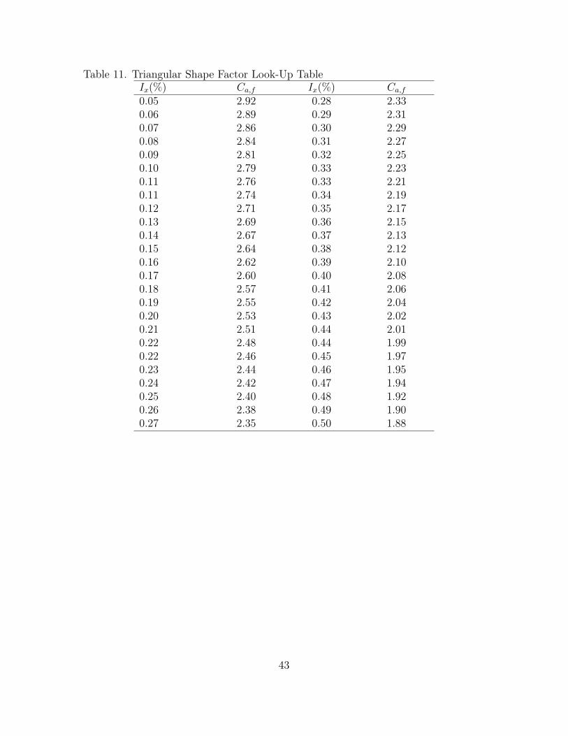
Table 11. Triangular Shape Factor Look-Up TableIx(%) Ca,f Ix(%) Ca,f0.05 2.92 0.28 2.330.06 2.89 0.29 2.310.07 2.86 0.30 2.290.08 2.84 0.31 2.270.09 2.81 0.32 2.250.10 2.79 0.33 2.230.11 2.76 0.33 2.210.11 2.74 0.34 2.190.12 2.71 0.35 2.170.13 2.69 0.36 2.150.14 2.67 0.37 2.130.15 2.64 0.38 2.120.16 2.62 0.39 2.100.17 2.60 0.40 2.080.18 2.57 0.41 2.060.19 2.55 0.42 2.040.20 2.53 0.43 2.020.21 2.51 0.44 2.010.22 2.48 0.44 1.990.22 2.46 0.45 1.970.23 2.44 0.46 1.950.24 2.42 0.47 1.940.25 2.40 0.48 1.920.26 2.38 0.49 1.900.27 2.35 0.50 1.88
43

APPENDIX E
CURVE FITTING STATISTICS
44
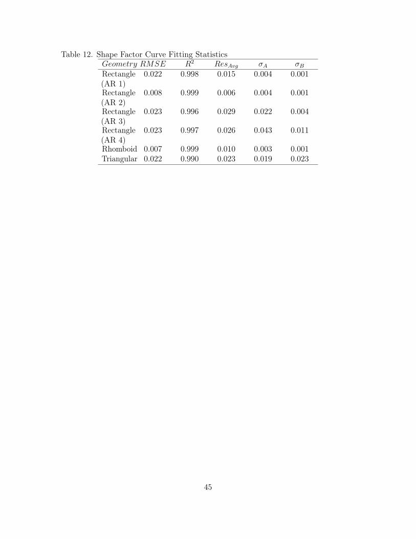
Table 12. Shape Factor Curve Fitting StatisticsGeometry RMSE R2 ResAvg σA σBRectangle(AR 1)
0.022 0.998 0.015 0.004 0.001
Rectangle(AR 2)
0.008 0.999 0.006 0.004 0.001
Rectangle(AR 3)
0.023 0.996 0.029 0.022 0.004
Rectangle(AR 4)
0.023 0.997 0.026 0.043 0.011
Rhomboid 0.007 0.999 0.010 0.003 0.001Triangular 0.022 0.990 0.023 0.019 0.023
45