1

Shannon Kelly Econometrics Research Paper on CEO Salaries

Reflection of CEO Salary Related to a Company’s Net Income in 1990 1. INTRODUCTION

I would like to study the relationship between CEO salary in 1990, the Net Income of the company in 1990, in addition to the Return on Capital (ROK) in 1990. This is because I believe that if there are positive values of net income and ROK than we should see positive CEO salary. Therefore, in my study CEO salary will be my dependent variable. The return on capital is also calculated by including the value of net income of a company and therefore relate to one another, I expect them to be positively correlated.

𝑅𝑒𝑡𝑢𝑟𝑛𝑜𝑛𝐶𝑎𝑝𝑖𝑡𝑎𝑙 = 𝑁𝑒𝑡𝐼𝑛𝑐𝑜𝑚𝑒 − 𝐷𝑖𝑣𝑖𝑑𝑒𝑛𝑑𝑠

𝑇𝑜𝑡𝑎𝑙𝐶𝑎𝑝𝑖𝑡𝑎𝑙

CEO salary naturally should be a reflection of a company’s productivity because if

companies are doing well it is with confidence that it is a result of the CEO’s hard work (McClure, 2004). I believe that CEO salaries are extremely large based on what I see in the media and how the injustice is portrayed in the difference between CEO salaries in comparison to the employee salaries working for the same company. Alternatively, “In any discussion of executive compensation it must be remembered that many reports in the news media focus on extreme cases, and that the compensation for executives of the top-200 companies is likely to be much higher than for smaller companies…” (EBSCO Host). This challenges my belief about CEO salaries because it makes sense for the media to exaggerate the truth with the most striking CEO salary values that can be found. The textbook analysis of CEO salary stems from the notion that CEO salary should be a reflection of the positive performance of a corporation. Based on a study done in 1990 and posted in 2014 online, authors Michael Jensen and Kevin Murphy claim that, “In most publicly held companies, the compensation of top executives is virtually independent of performance” (Jensen, Murphy, 2014). The base of their data comes from information on salaries and bonuses for 2,505 CEOs in 1,400 publicly held companies from 1974 through 1988 (Jensen, Murphy, 2014). Their data is reliable relating to the inference they make leading into the 1990’s considering that 1988 is only two years prior to the data that I am looking at. Additionally, Jensen and Murphy collected data on stock options and stock ownership for CEOs of the 430 largest publicly held companies in 1988 (Jensen, Murphy, 2014).

I want to focus my research on CEO salary in 1990 around the return on invested capital in 1990 because it is an assessment of a company’s efficiency in the way it allocates its own controlled capital (Investopedia). There should be a positive relationship between CEO salary in 1990 if the return on capital as well as net income were positive for 1990. I do not believe that CEO salary will be significantly larger if net income, return on capital and equity, etc. are negative because, “The most powerful link between shareholder wealth and executive wealth is direct stock ownership by the CEO.” (Jensen, Murphy, 2014). “Shareholders rely on CEOs to adopt policies that maximize the value of their shares.” (Jensen, Murphy, 2014). This implies that CEOs are incentivized to be productive and help benefit the company when their own personal finances are invested into it. This claim is also supported by EBSCO because CEO compensation does not only

2

come from their paychecks but, “Most important is the value of stock options, which give executives the right to buy shares in a corporation at a given moment at the price the hare was sold for on that day” (EBSCO). This means that CEOs have an unfair advantage in the way that they can buy their shares in other companies and can gain a profit others do not have access to. I will take the ‘stock price 1990’ variable into consideration in my research because it may control for my main x-values and y-value I am interested in.

Understanding the relationship between CEO salary and the profitability of a company is of great importance and has implications on the analysis of social inequalities; many people are under the impression that CEO’s have reckless incomes and are able to continuously make excessive profits off of the companies they lead without the company itself prospering. Jensen and Murphy at the time found that, “…for the median CEO in the 250 largest companies, a $1,000 change in corporate value corresponds to a change of just 6.7 cents in salary and bonus over two years.” (Jensen, Murphy, 2014) This implies that the profitability of a company does not substantially influence an increase in the salary or bonus of the CEOs of those companies. The data used is relevant to the 1990s and therefore may not reflect the magnitude of financial wealth some CEOs see today but we can still understand how CEO salary might have been measured at that time.

The contribution of this study is to further explore with my own data a few years ahead of Jensen and Murphy to see if their assertions and conclusions are reliable. I’m not fully convinced that CEO salaries are not significantly larger with respect to the profitability or unprofitability of a company. According to EBSCO, the average chief executive earned close to 40 times more than the average employee but by 1990 the average CEO was earning 107 times as much. I analyze the relationship between the logarithm of net income and the logarithm of CEO salary in 1990 (EBSCO). I find that more profitable companies should have CEOs with higher salaries in comparison to companies with smaller logarithms of net income values. In considering data from 1990 should show on its own high values of CEO salaries regardless of the other variables being considered. 2. DATA

The dataset included in the research is titled, “RETURN.dta” that accounts for 142 observations for the 12 variables that represents cross-sectional data on CEO salaries. The data gives samples for return on equity (ROE) and capital (ROK) from 1990 in addition to other variables that account for years 1990 and 1994. I can compare values form 1990 and 1994 to anticipate an increase or decrease in CEO salary, for example, in the future. ROE is a measure of profitability that calculates how many dollars of profit a company generate with each dollar of shareholders’ equity. Formula for ROE is Roe = Net Income/Shareholders’ Equity, ROE also can be referred to as “return on net worth.” ROK (ROC), or return on invest capital (ROIC), is a ratio used in finance, valuation and accounting, as a measure of the profitability and value-creating potential of companies after taking into account the amount of initial capital invested. Equity is the owner’s share of the assets of a business while capital is the owner’s investment of assets in a business. The debt-to-capital ratio is a measurement of a company’s financial leverage. The debt-to-capital ratio is calculated by taking the company’s debt, including both short and long term liabilities and dividing it by the total capital. Total capital is all debt plus shareholders’ equity. The higher the ratio the more the company uses debt to finance its operation. A high ratio means the company is at a higher risk for bankruptcy. A company with a low ratio finances with equity. Referring to Table 1, it is interesting

3

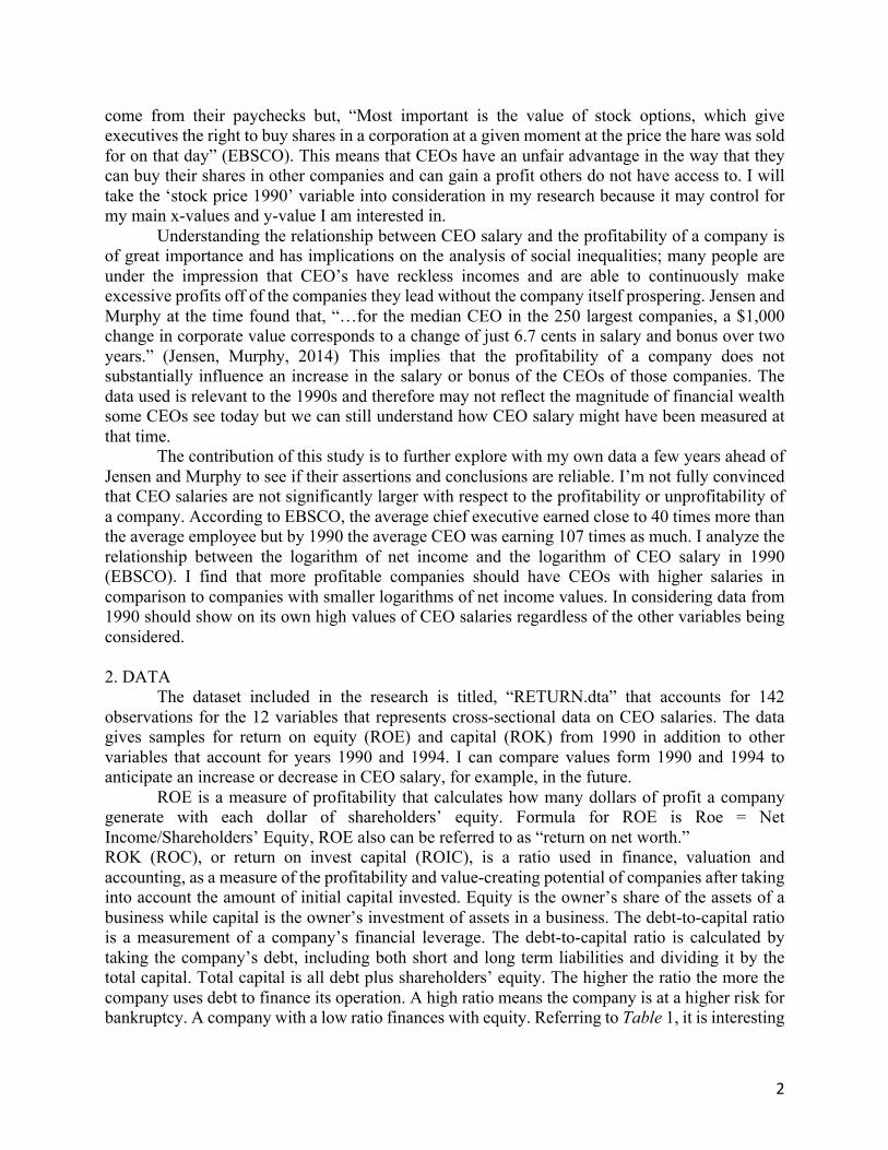
that the average for the logarithms of net income and CEO salary are fairly similar but the CEO salary average is larger than net income average of companies. Table1 Summary of Data Set Variables

3. DESCRIPTIVE STATISTICS: TABLES AND GRAPHICS

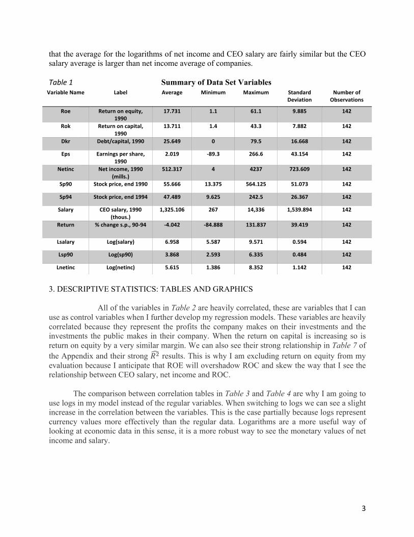
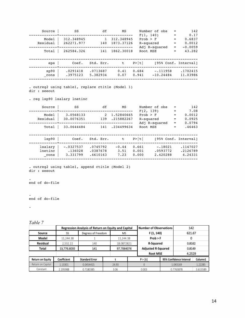
All of the variables in Table 2 are heavily correlated, these are variables that I can use as control variables when I further develop my regression models. These variables are heavily correlated because they represent the profits the company makes on their investments and the investments the public makes in their company. When the return on capital is increasing so is return on equity by a very similar margin. We can also see their strong relationship in Table 7 of the Appendix and their strong 𝑅9 results. This is why I am excluding return on equity from my evaluation because I anticipate that ROE will overshadow ROC and skew the way that I see the relationship between CEO salary, net income and ROC.

The comparison between correlation tables in Table 3 and Table 4 are why I am going to use logs in my model instead of the regular variables. When switching to logs we can see a slight increase in the correlation between the variables. This is the case partially because logs represent currency values more effectively than the regular data. Logarithms are a more useful way of looking at economic data in this sense, it is a more robust way to see the monetary values of net income and salary.

VariableName Label Average Minimum Maximum StandardDeviation

NumberofObservations

Roe Returnonequity,1990

17.731 1.1 61.1 9.885 142

Rok Returnoncapital,1990

13.711 1.4 43.3 7.882 142

Dkr Debt/capital,1990 25.649 0 79.5 16.668 142

Eps Earningspershare,1990

2.019 -89.3 266.6 43.154 142

Netinc Netincome,1990(mills.)

512.317 4 4237 723.609 142

Sp90 Stockprice,end1990 55.666 13.375 564.125 51.073 142

Sp94 Stockprice,end1994 47.489 9.625 242.5 26.367 142

Salary CEOsalary,1990(thous.)

1,325.106 267 14,336 1,539.894 142

Return %changes.p.,90-94 -4.042 -84.888 131.837 39.419 142

Lsalary Log(salary) 6.958 5.587 9.571 0.594 142

Lsp90 Log(sp90) 3.868 2.593 6.335 0.484 142

Lnetinc Log(netinc) 5.615 1.386 8.352 1.142 142

4

Figure 1 on log(salary) of CEOs depicts a more accurate frequency distribution in regards

to income where we can see that close to 30% of CEO’s have salaries above $1 million. The log of 7 is ~$1,000 and then we need to consider this in thousands, 1,000 x 1,000 = $1 million.

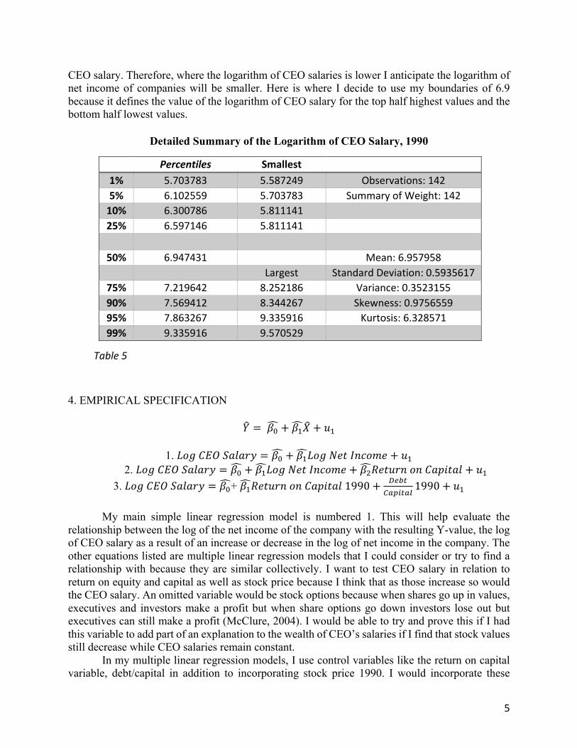
Table 5 is important because it shows the percentile separation of the logarithm of CEO salary, 1990 and how the logarithms of their salaries are divided into lower to higher percentage values. I am going to use this in my regression model for specific restrictions on the value of CEO salaries in logarithms in regard to the logarithm of net income. This relates to my hypothesis because I believe that with a higher net income of a company I anticipate that there will be a higher

0.2

.4.6

.8Fr

actio

n

6 7 8 9 10log(salary)

Histogram Log(Salary)

2 EarningsperShare ReturnonCapital ReturnonEquity

EarningsperShare 1

ReturnonCapital 0.5187 1 ReturnonEquity 0.5201 0.9034 1

Table2

3 Salary NetIncome EarningsperShareSalary 1

NetIncome 0.1826 1 EarningsperShare 0.124 0.0976 1

Table3

4 LogSalary LogNetIncome ReturnonCapital

LogSalary 1

LogNetIncome 0.4676 1 ReturnonCapital 0.1345 0.1631 1

Table4

Figure1

5

CEO salary. Therefore, where the logarithm of CEO salaries is lower I anticipate the logarithm of net income of companies will be smaller. Here is where I decide to use my boundaries of 6.9 because it defines the value of the logarithm of CEO salary for the top half highest values and the bottom half lowest values.

Detailed Summary of the Logarithm of CEO Salary, 1990

4. EMPIRICAL SPECIFICATION

𝑌 = 𝛽< + 𝛽>𝑋 + 𝑢>

1. 𝐿𝑜𝑔𝐶𝐸𝑂𝑆𝑎𝑙𝑎𝑟𝑦 = 𝛽< + 𝛽>𝐿𝑜𝑔𝑁𝑒𝑡𝐼𝑛𝑐𝑜𝑚𝑒 + 𝑢> 2. 𝐿𝑜𝑔𝐶𝐸𝑂𝑆𝑎𝑙𝑎𝑟𝑦 = 𝛽< + 𝛽>𝐿𝑜𝑔𝑁𝑒𝑡𝐼𝑛𝑐𝑜𝑚𝑒 + 𝛽9𝑅𝑒𝑡𝑢𝑟𝑛𝑜𝑛𝐶𝑎𝑝𝑖𝑡𝑎𝑙 + 𝑢>

3. 𝐿𝑜𝑔𝐶𝐸𝑂𝑆𝑎𝑙𝑎𝑟𝑦 = 𝛽<+ 𝛽>𝑅𝑒𝑡𝑢𝑟𝑛𝑜𝑛𝐶𝑎𝑝𝑖𝑡𝑎𝑙1990 +IJKL

MNOPLNQ1990 + 𝑢>

My main simple linear regression model is numbered 1. This will help evaluate the

relationship between the log of the net income of the company with the resulting Y-value, the log of CEO salary as a result of an increase or decrease in the log of net income in the company. The other equations listed are multiple linear regression models that I could consider or try to find a relationship with because they are similar collectively. I want to test CEO salary in relation to return on equity and capital as well as stock price because I think that as those increase so would the CEO salary. An omitted variable would be stock options because when shares go up in values, executives and investors make a profit but when share options go down investors lose out but executives can still make a profit (McClure, 2004). I would be able to try and prove this if I had this variable to add part of an explanation to the wealth of CEO’s salaries if I find that stock values still decrease while CEO salaries remain constant. In my multiple linear regression models, I use control variables like the return on capital variable, debt/capital in addition to incorporating stock price 1990. I would incorporate these

Percentiles Smallest 1% 5.703783 5.587249 Observations:1425% 6.102559 5.703783 SummaryofWeight:14210% 6.300786 5.811141 25% 6.597146 5.811141

50% 6.947431 Mean:6.957958 Largest StandardDeviation:0.5935617

75% 7.219642 8.252186 Variance:0.352315590% 7.569412 8.344267 Skewness:0.975655995% 7.863267 9.335916 Kurtosis:6.32857199% 9.335916 9.570529

Table5

6

variables because the ROK (ROC) is partially a result of net income and I would anticipate that when the log of net income increases so would the return on capital. Using this as a control will allow me to evaluate the change in CEO salary, if any. Additionally, when stock price is higher the stock is riskier but generates a higher return for the shareholders. Generally, as an incentive CEOs may be required to invest in their own companies and, “The most powerful link between shareholder wealth and executive wealth is direct ownership of shares by the CEO.” (Jensen, Murphy, 2014). If stock price is higher the earnings per share could also be higher. If they are not, then this implies that the risky stock with a higher price was not generating the return that shareholders anticipated. This could reflect a negative downturn for CEO salary as well as negative net income for a particular company because if the company is a riskier stock they might not see a profitability from their stock. Additionally, putting their own capital into their company’s stock if it is not doing well could negatively impact return on capital. I anticipate that all the coefficients for these variables will be positive unless the data set observations for return on capital demonstrate that the companies were not efficiently investing their capital and therefore that variables may have a negative coefficient that would decreases the net income of the company and minimize the log of CEO salary. I will also do simple linear regressions for the logarithm of salary greater than 6.9 and less than 6.9 based on the lower and upper 50% of CEO salary values as seen in Table 5 to more closely evaluate the effect of net income on the logarithm of salary. 5. RESULTS Dependentvariable:logarithmofCEOSalary,1990Regressor (1) (2) (3) (4) (5) (6)

LogarithmNetIncome 0.243***(0.0388)

0.238***(0.0398)

0.243***(0.0404)

0.236***(0.0414)

ReturnonCapital,1990 0.00451(0.00565)

0.00605(0.00675)

0.00601(0.00678)

Debt/Capital,1990 -0.00136(0.00240)

0.00130(0.00319)

StockPrice,end1990 -0.000168(0.000895)

Lnetinciflsalary<6.9 0.0838**(0.0397)

Lnetinciflsalary≥6.9 0.0896*(0.0492)

Intercept 5.593*** 5.559*** 5.525*** 5.527*** 6.057*** 6.805***

F-statisticsandSummaryStatistics

NumberofObservations

142 142 142 142 64 78

F-statistics(p-value) 19.85(0)

13.22(0)

9.85(0)

𝑅9 0.219 0.222 0.219 0.223 0.067 0.041

Standarderrorsaregiveninparenthesesundercoefficients,andp-valuesaregiveninparenthesesunderF-statistics.Individualcoefficientsarestatisticallysignificantatthe*10%,**5%,or***1%significancelevel.

7

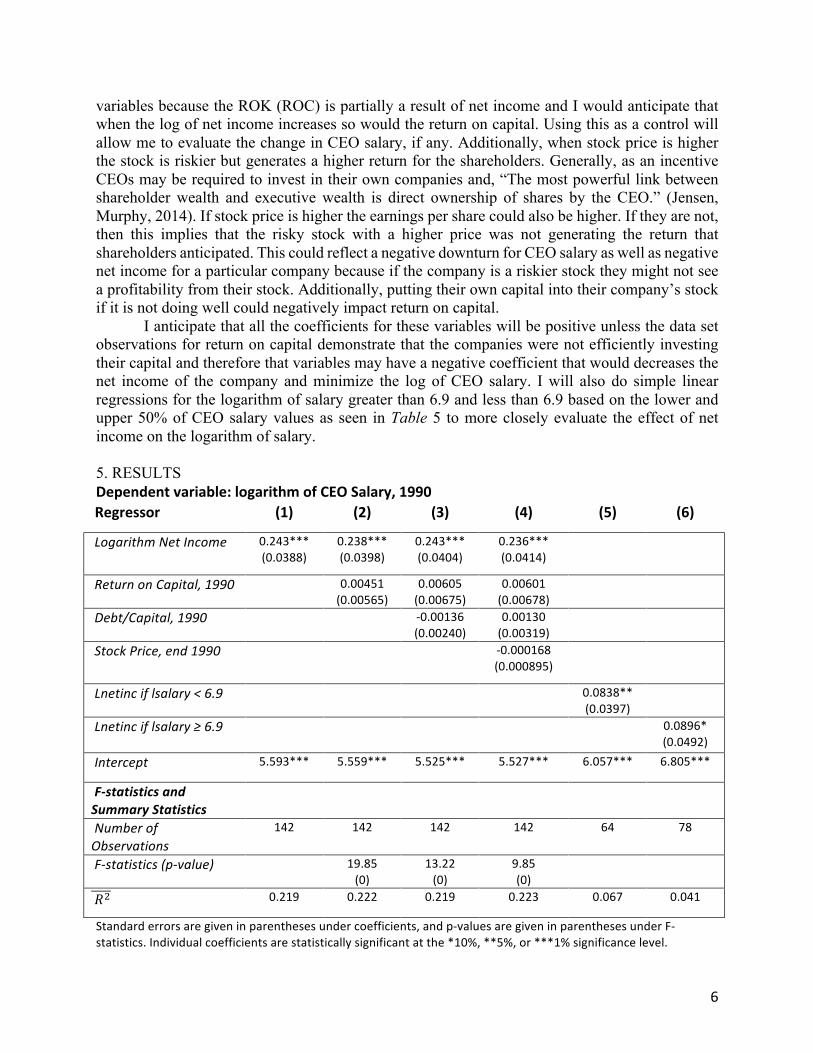
My strongest coefficient throughout all the regression models as seen in Table 6 was the logarithm of net income. As I hypothesize, the coefficient is positive and relates to a marginal increase in the logarithm of CEO’s salary in 1990. Model 1 of the simple linear model had a decent 𝑅9values that depicts some of data in this model is statistically represented appropriately. Additionally, our data for the logarithm of net income is statistically significant at a 1% significance, or with 99% confidence we can reject the null that or variable is equal to zero. Therefore, these variables are related, as anticipated.

Model 2 in Table 6 turns to a multiple linear regression model that includes the return on capital. We can see that our lnetinc coefficient slightly decreases when the ROK is included but it is not a drastic change. Our coefficient for lnetinc is still statistically significant at a 1% significance level but our ROK coefficient is not significant at a 10%, 5% or 1% level. From this point I wanted to do and f-test to see if lnetinc and ROK are statistically significant together in a joint hypothesis test or if the f-test would depict that these variables together are not statistically significant from 0. The f-statistic result for Model 2 seen in Table 6 is actually fairly significant and has p-value of 0, therefore this multiple linear regression model is not insignificant. ROK alone in this model has a standard error that is greater than the value of its coefficient and therefore is very miniscule in its impact on lsalary.

Continuing onto Model 3 in Table 6 the variable debt/capital, 1990 was added to the multiple linear regression where we see the coefficient for ROK increased but its standard error is still larger than the coefficient and the coefficient for the dkr is negative. The absolute value of the coefficient of dkr is also still smaller than its standard error. Ultimately, these variables do not seem to have a significant relationship with the lsalary of CEOs but again the f-test implies otherwise based on their joint hypothesis test. The 𝑅9for Model 2 and 3 are also not poor, even though 𝑅9does not define the significance of these variables it does imply a weak but still present relationship between them all.

Model 4 in Table 6 was the last multiple linear regression model which added the stock price in 1990, which has a negative coefficient and a standard error larger than the coefficient itself. What is interested to note is that the coefficient for the dkr variable is no longer negative but its standard error is larger than before. I used the dkr as a control variable because the higher the debt-to-capital ratio the risker the company. Therefore, I was anticipating it would have a negative effect on the CEO salary and should show a decrease in their salary if the company is riskier. Ultimately, this variable proved to have little relationship with the log of CEO salary and the other variables included. The stock price of 1990 was another control variable that I was hoping could be a measurement related to CEO salary. A higher stock price entails that the company is a safe investment and therefore the shareholders will see themselves with a nicer payoff (Pinsent). In contrast a cheaper stock price tends to signal a riskier investment so I anticipated that the stock price for 1990 should have a positive coefficient therefore when the value is higher it would have a greater positive impact on CEO salary. This is because with more capital investment in a company would mean that the company is profitable and the CEO salary would reflect some of that benefit. Alternatively, the coefficient, even though extremely small, was a negative value implying that with higher stock price there would be a more negative effect on the CEO salary. The variables for Models 1, 2,3, and 4 do not pass any confidence interval test aside from the log of netinc variable. Therefore, it cannot be confirmed that the others are statistically significant from zero and does not make me very confident in any of the multiple linear regression models because there’s not much proof that they are dependable. After running and f-test for Model 4 its f-statistic was not insignificant and the p-value was 0, but that also doesn’t make me very much

8

more convinced that those model effectively represent and controlled representation of factors that affect the log of CEO salary in 1990.

Models 5 and 6 were linear regression models that used information from Table 5 that reflected the highest salaries in logarithms and the lowest percentage of salaries. I divided the logarithm of salaries in the higher 50% and the lower 50%, therefore the log of CEO salary in 1990 was still the dependent variable with the log to net income as the independent variable while I controlled for a specific upper and lower range of salaries in terms of logarithms. I did this because I anticipated that I would see that based on the size of the companies and their log of net income we would see that with higher salaries we would see that higher log of net income relationship. Ultimately there was a small difference between the coefficients for the higher and lower ranges of salaries and did not show any stronger difference between the models. There were only 64 observations for the smaller range of salaries and 78 for the larger range so there are the same amount of observations being accounted for the regression, you would thing Model 6 would be stronger since it has more observations. When comparing the 𝑅9values for Models 5 and 6 it actually appears that Model 5 represents its data more effectively than Model 6. The 𝑅9value for both Model 5 and 6 are far smaller than what we see for all the other models and does not make a strong argument for the case that higher values of salary have a stronger positive relationship with a higher log of net income. There is a small marginal difference between the two.

6. DISCUSSION AND CONCLUSION My models appear to confirm the study done on CEO salaries in 1990 by Michael Jensen and Kevin Murphy. This is because they explained that the reality of CEO salaries was not that they were extremely large in comparison the profitability of their companies. It is hard to measure CEO salaries and company size when there is not a variable to control for the size of companies. If there were a binary variable included in the data set that was 1 if large company and 0 if small company then I may be able to determine the variability between CEO salary and the actual profitability of a company, if their stock prices were correlated with that and if smaller companies had more debt and therefore CEO salaries suffered. What I found most interesting in their study was their comments that, “The relentless focus on how much CEOs are paid diverts public attention from the real problem-how CEOs are paid” (Jensen, Murphy, 2014). Myself included, I did not understand how CEOs actually got paid but just assumed that it was and outstanding unfair amount that was at the expense of the companies they work for. Their study contained information of CEO salaries that expanded on five decades of collected information where I only had access to 1990 and 1994 where I did not include the 1994 based on the focus I wanted my study to have. Also information like what stocks CEOs owned and if they owned a share of their own company’s stock, also if there were publicly or privately owned companies and use that as a control on the magnitude of a CEOs salary as well as if they received benefits like bonuses. “More aggressive pay-for-performance systems (and a higher probability of dismissal for poor performance) would produce sharply lower compensation for less talented manager” (Jensen, Murphy, 2014). I think having a measurement for a CEOs performance as a marker for the relationship for their salary would also be useful information to have. Jensen and Murphy are able to acknowledge that it is not just a given that CEO salaries are going to be exponentially higher than any other financial factors in their companies; that they will have high compensation even if the company is doing poorly. I agree with their research and think that if anything that I contributed it was that now I agree for myself that CEO salary is determined off of many other varying factors. Additionally, a CEO may not be incentivized enough to make a valuable impact for a company because the amount of work

9

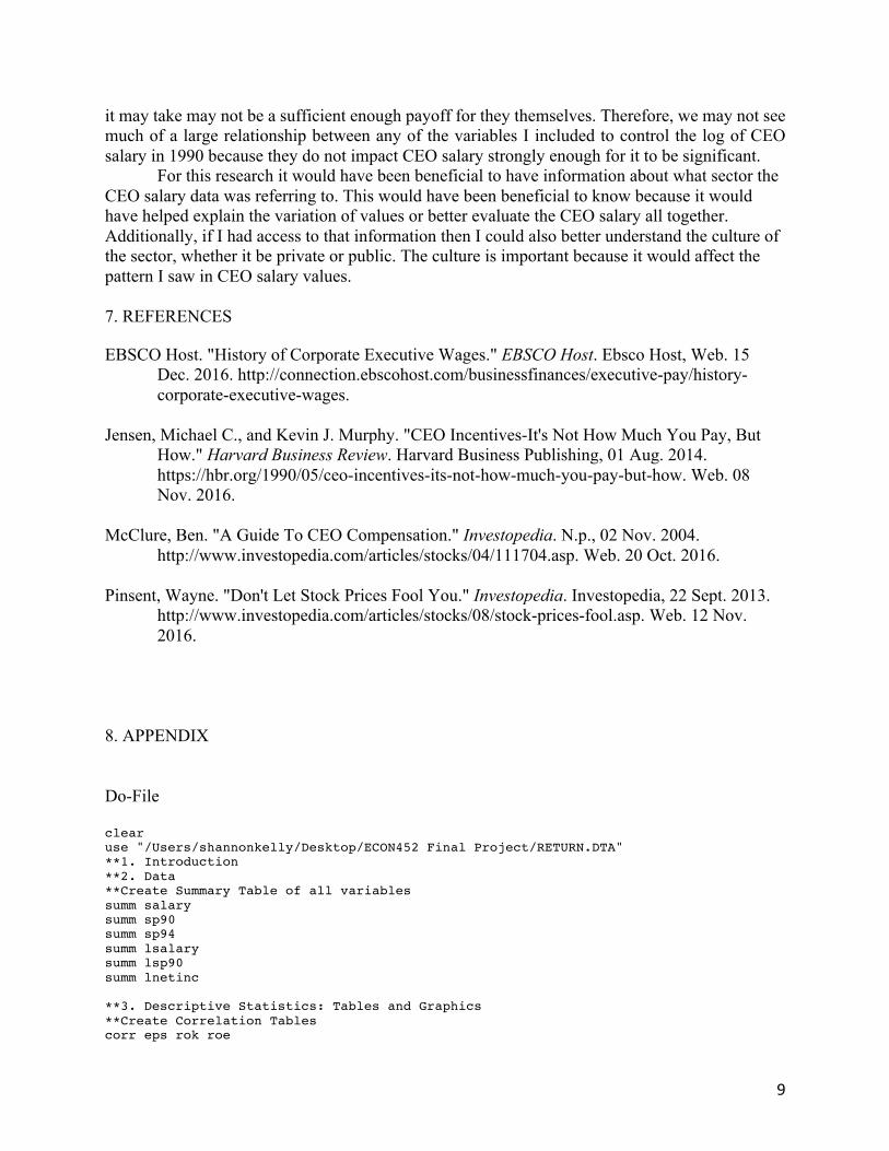
it may take may not be a sufficient enough payoff for they themselves. Therefore, we may not see much of a large relationship between any of the variables I included to control the log of CEO salary in 1990 because they do not impact CEO salary strongly enough for it to be significant. For this research it would have been beneficial to have information about what sector the CEO salary data was referring to. This would have been beneficial to know because it would have helped explain the variation of values or better evaluate the CEO salary all together. Additionally, if I had access to that information then I could also better understand the culture of the sector, whether it be private or public. The culture is important because it would affect the pattern I saw in CEO salary values. 7. REFERENCES EBSCO Host. "History of Corporate Executive Wages." EBSCO Host. Ebsco Host, Web. 15

Dec. 2016. http://connection.ebscohost.com/businessfinances/executive-pay/history-corporate-executive-wages.

Jensen, Michael C., and Kevin J. Murphy. "CEO Incentives-It's Not How Much You Pay, But

How." Harvard Business Review. Harvard Business Publishing, 01 Aug. 2014. https://hbr.org/1990/05/ceo-incentives-its-not-how-much-you-pay-but-how. Web. 08 Nov. 2016.

McClure, Ben. "A Guide To CEO Compensation." Investopedia. N.p., 02 Nov. 2004.

http://www.investopedia.com/articles/stocks/04/111704.asp. Web. 20 Oct. 2016. Pinsent, Wayne. "Don't Let Stock Prices Fool You." Investopedia. Investopedia, 22 Sept. 2013.

http://www.investopedia.com/articles/stocks/08/stock-prices-fool.asp. Web. 12 Nov. 2016.

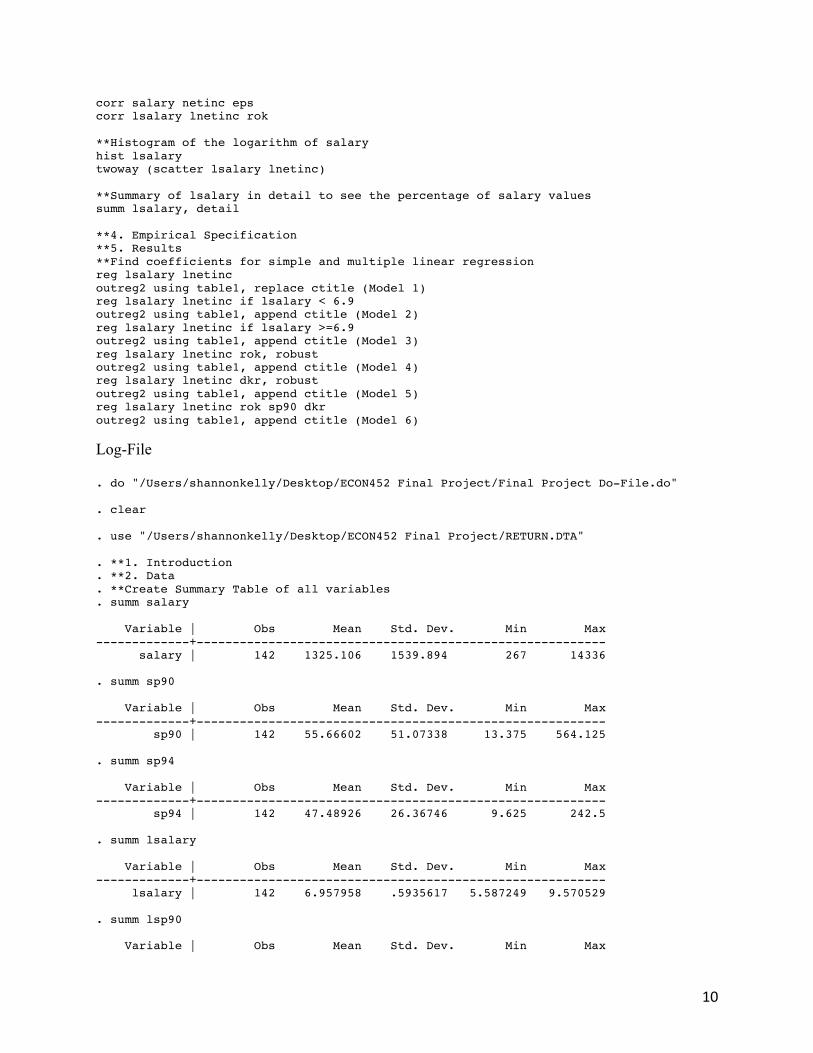
8. APPENDIX Do-File clear use "/Users/shannonkelly/Desktop/ECON452 Final Project/RETURN.DTA" **1. Introduction **2. Data **Create Summary Table of all variables summ salary summ sp90 summ sp94 summ lsalary summ lsp90 summ lnetinc **3. Descriptive Statistics: Tables and Graphics **Create Correlation Tables corr eps rok roe

10

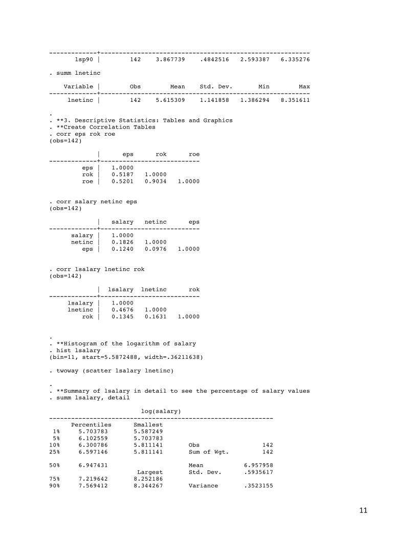
corr salary netinc eps corr lsalary lnetinc rok **Histogram of the logarithm of salary hist lsalary twoway (scatter lsalary lnetinc) **Summary of lsalary in detail to see the percentage of salary values summ lsalary, detail **4. Empirical Specification **5. Results **Find coefficients for simple and multiple linear regression reg lsalary lnetinc outreg2 using table1, replace ctitle (Model 1) reg lsalary lnetinc if lsalary < 6.9 outreg2 using table1, append ctitle (Model 2) reg lsalary lnetinc if lsalary >=6.9 outreg2 using table1, append ctitle (Model 3) reg lsalary lnetinc rok, robust outreg2 using table1, append ctitle (Model 4) reg lsalary lnetinc dkr, robust outreg2 using table1, append ctitle (Model 5) reg lsalary lnetinc rok sp90 dkr outreg2 using table1, append ctitle (Model 6) Log-File . do "/Users/shannonkelly/Desktop/ECON452 Final Project/Final Project Do-File.do" . clear . use "/Users/shannonkelly/Desktop/ECON452 Final Project/RETURN.DTA" . **1. Introduction . **2. Data . **Create Summary Table of all variables . summ salary Variable | Obs Mean Std. Dev. Min Max -------------+--------------------------------------------------------- salary | 142 1325.106 1539.894 267 14336 . summ sp90 Variable | Obs Mean Std. Dev. Min Max -------------+--------------------------------------------------------- sp90 | 142 55.66602 51.07338 13.375 564.125 . summ sp94 Variable | Obs Mean Std. Dev. Min Max -------------+--------------------------------------------------------- sp94 | 142 47.48926 26.36746 9.625 242.5 . summ lsalary Variable | Obs Mean Std. Dev. Min Max -------------+--------------------------------------------------------- lsalary | 142 6.957958 .5935617 5.587249 9.570529 . summ lsp90 Variable | Obs Mean Std. Dev. Min Max

11

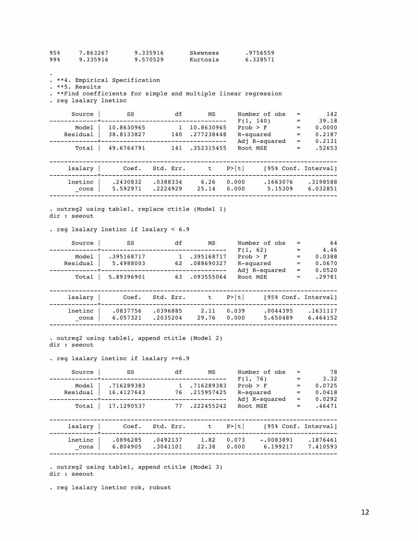
-------------+--------------------------------------------------------- lsp90 | 142 3.867739 .4842516 2.593387 6.335276 . summ lnetinc Variable | Obs Mean Std. Dev. Min Max -------------+--------------------------------------------------------- lnetinc | 142 5.615309 1.141858 1.386294 8.351611 . . **3. Descriptive Statistics: Tables and Graphics . **Create Correlation Tables . corr eps rok roe (obs=142) | eps rok roe -------------+--------------------------- eps | 1.0000 rok | 0.5187 1.0000 roe | 0.5201 0.9034 1.0000 . corr salary netinc eps (obs=142) | salary netinc eps -------------+--------------------------- salary | 1.0000 netinc | 0.1826 1.0000 eps | 0.1240 0.0976 1.0000 . corr lsalary lnetinc rok (obs=142) | lsalary lnetinc rok -------------+--------------------------- lsalary | 1.0000 lnetinc | 0.4676 1.0000 rok | 0.1345 0.1631 1.0000 . . **Histogram of the logarithm of salary . hist lsalary (bin=11, start=5.5872488, width=.36211638) . twoway (scatter lsalary lnetinc) . . **Summary of lsalary in detail to see the percentage of salary values . summ lsalary, detail log(salary) ------------------------------------------------------------- Percentiles Smallest 1% 5.703783 5.587249 5% 6.102559 5.703783 10% 6.300786 5.811141 Obs 142 25% 6.597146 5.811141 Sum of Wgt. 142 50% 6.947431 Mean 6.957958 Largest Std. Dev. .5935617 75% 7.219642 8.252186 90% 7.569412 8.344267 Variance .3523155

12

95% 7.863267 9.335916 Skewness .9756559 99% 9.335916 9.570529 Kurtosis 6.328571 . . **4. Empirical Specification . **5. Results . **Find coefficients for simple and multiple linear regression . reg lsalary lnetinc Source | SS df MS Number of obs = 142 -------------+---------------------------------- F(1, 140) = 39.18 Model | 10.8630965 1 10.8630965 Prob > F = 0.0000 Residual | 38.8133827 140 .277238448 R-squared = 0.2187 -------------+---------------------------------- Adj R-squared = 0.2131 Total | 49.6764791 141 .352315455 Root MSE = .52653 ------------------------------------------------------------------------------ lsalary | Coef. Std. Err. t P>|t| [95% Conf. Interval] -------------+---------------------------------------------------------------- lnetinc | .2430832 .0388334 6.26 0.000 .1663076 .3198588 _cons | 5.592971 .2224929 25.14 0.000 5.15309 6.032851 ------------------------------------------------------------------------------ . outreg2 using table1, replace ctitle (Model 1) dir : seeout . reg lsalary lnetinc if lsalary < 6.9 Source | SS df MS Number of obs = 64 -------------+---------------------------------- F(1, 62) = 4.46 Model | .395168717 1 .395168717 Prob > F = 0.0388 Residual | 5.4988003 62 .088690327 R-squared = 0.0670 -------------+---------------------------------- Adj R-squared = 0.0520 Total | 5.89396901 63 .093555064 Root MSE = .29781 ------------------------------------------------------------------------------ lsalary | Coef. Std. Err. t P>|t| [95% Conf. Interval] -------------+---------------------------------------------------------------- lnetinc | .0837756 .0396885 2.11 0.039 .0044395 .1631117 _cons | 6.057321 .2035204 29.76 0.000 5.650489 6.464152 ------------------------------------------------------------------------------ . outreg2 using table1, append ctitle (Model 2) dir : seeout . reg lsalary lnetinc if lsalary >=6.9 Source | SS df MS Number of obs = 78 -------------+---------------------------------- F(1, 76) = 3.32 Model | .716289383 1 .716289383 Prob > F = 0.0725 Residual | 16.4127643 76 .215957425 R-squared = 0.0418 -------------+---------------------------------- Adj R-squared = 0.0292 Total | 17.1290537 77 .222455242 Root MSE = .46471 ------------------------------------------------------------------------------ lsalary | Coef. Std. Err. t P>|t| [95% Conf. Interval] -------------+---------------------------------------------------------------- lnetinc | .0896285 .0492137 1.82 0.073 -.0083891 .1876461 _cons | 6.804905 .3041101 22.38 0.000 6.199217 7.410593 ------------------------------------------------------------------------------ . outreg2 using table1, append ctitle (Model 3) dir : seeout . reg lsalary lnetinc rok, robust

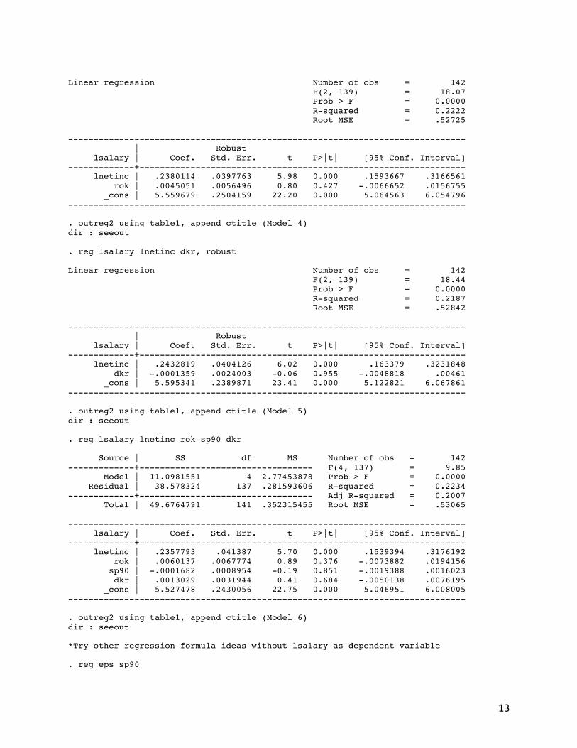
13

Linear regression Number of obs = 142 F(2, 139) = 18.07 Prob > F = 0.0000 R-squared = 0.2222 Root MSE = .52725 ------------------------------------------------------------------------------ | Robust lsalary | Coef. Std. Err. t P>|t| [95% Conf. Interval] -------------+---------------------------------------------------------------- lnetinc | .2380114 .0397763 5.98 0.000 .1593667 .3166561 rok | .0045051 .0056496 0.80 0.427 -.0066652 .0156755 _cons | 5.559679 .2504159 22.20 0.000 5.064563 6.054796 ------------------------------------------------------------------------------ . outreg2 using table1, append ctitle (Model 4) dir : seeout . reg lsalary lnetinc dkr, robust Linear regression Number of obs = 142 F(2, 139) = 18.44 Prob > F = 0.0000 R-squared = 0.2187 Root MSE = .52842 ------------------------------------------------------------------------------ | Robust lsalary | Coef. Std. Err. t P>|t| [95% Conf. Interval] -------------+---------------------------------------------------------------- lnetinc | .2432819 .0404126 6.02 0.000 .163379 .3231848 dkr | -.0001359 .0024003 -0.06 0.955 -.0048818 .00461 _cons | 5.595341 .2389871 23.41 0.000 5.122821 6.067861 ------------------------------------------------------------------------------ . outreg2 using table1, append ctitle (Model 5) dir : seeout . reg lsalary lnetinc rok sp90 dkr Source | SS df MS Number of obs = 142 -------------+---------------------------------- F(4, 137) = 9.85 Model | 11.0981551 4 2.77453878 Prob > F = 0.0000 Residual | 38.578324 137 .281593606 R-squared = 0.2234 -------------+---------------------------------- Adj R-squared = 0.2007 Total | 49.6764791 141 .352315455 Root MSE = .53065 ------------------------------------------------------------------------------ lsalary | Coef. Std. Err. t P>|t| [95% Conf. Interval] -------------+---------------------------------------------------------------- lnetinc | .2357793 .041387 5.70 0.000 .1539394 .3176192 rok | .0060137 .0067774 0.89 0.376 -.0073882 .0194156 sp90 | -.0001682 .0008954 -0.19 0.851 -.0019388 .0016023 dkr | .0013029 .0031944 0.41 0.684 -.0050138 .0076195 _cons | 5.527478 .2430056 22.75 0.000 5.046951 6.008005 ------------------------------------------------------------------------------ . outreg2 using table1, append ctitle (Model 6) dir : seeout *Try other regression formula ideas without lsalary as dependent variable . reg eps sp90

14

Source | SS df MS Number of obs = 142 -------------+---------------------------------- F(1, 140) = 0.17 Model | 312.348945 1 312.348945 Prob > F = 0.6837 Residual | 262271.977 140 1873.37126 R-squared = 0.0012 -------------+---------------------------------- Adj R-squared = -0.0059 Total | 262584.326 141 1862.30018 Root MSE = 43.282 ------------------------------------------------------------------------------ eps | Coef. Std. Err. t P>|t| [95% Conf. Interval] -------------+---------------------------------------------------------------- sp90 | .0291418 .0713687 0.41 0.684 -.111958 .1702415 _cons | .3975123 5.382934 0.07 0.941 -10.24484 11.03986 ------------------------------------------------------------------------------ . outreg2 using table1, replace ctitle (Model 1) dir : seeout . reg lsp90 lsalary lnetinc Source | SS df MS Number of obs = 142 -------------+---------------------------------- F(2, 139) = 7.08 Model | 3.0568133 2 1.52840665 Prob > F = 0.0012 Residual | 30.0076351 139 .215882267 R-squared = 0.0925 -------------+---------------------------------- Adj R-squared = 0.0794 Total | 33.0644484 141 .234499634 Root MSE = .46463 ------------------------------------------------------------------------------ lsp90 | Coef. Std. Err. t P>|t| [95% Conf. Interval] -------------+---------------------------------------------------------------- lsalary | -.0327537 .0745792 -0.44 0.661 -.18021 .1147027 lnetinc | .136028 .0387678 3.51 0.001 .0593772 .2126789 _cons | 3.331799 .4610163 7.23 0.000 2.420288 4.24331 ------------------------------------------------------------------------------ . outreg2 using table1, append ctitle (Model 2) dir : seeout . end of do-file . end of do-file . Table 7