Embed Size (px)
Citation preview

IZA DP No. 1043
Shadow Economies around the World:What Do We Know?
Friedrich SchneiderRobert Klinglmair
DI
SC
US
SI
ON
PA
PE
R S
ER
IE
S
Forschungsinstitutzur Zukunft der ArbeitInstitute for the Studyof Labor
March 2004

Shadow Economies around the World:
What Do We Know?
Friedrich Schneider University of Linz and IZA Bonn
Robert Klinglmair University of Linz
Discussion Paper No. 1043 March 2004
IZA
P.O. Box 7240 53072 Bonn
Germany
Phone: +49-228-3894-0 Fax: +49-228-3894-180
Email: [email protected]
Any opinions expressed here are those of the author(s) and not those of the institute. Research disseminated by IZA may include views on policy, but the institute itself takes no institutional policy positions. The Institute for the Study of Labor (IZA) in Bonn is a local and virtual international research center and a place of communication between science, politics and business. IZA is an independent nonprofit company supported by Deutsche Post World Net. The center is associated with the University of Bonn and offers a stimulating research environment through its research networks, research support, and visitors and doctoral programs. IZA engages in (i) original and internationally competitive research in all fields of labor economics, (ii) development of policy concepts, and (iii) dissemination of research results and concepts to the interested public. IZA Discussion Papers often represent preliminary work and are circulated to encourage discussion. Citation of such a paper should account for its provisional character. A revised version may be available on the IZA website (www.iza.org) or directly from the author.

IZA Discussion Paper No. 1043 March 2004
ABSTRACT
Shadow Economies around the World: What Do We Know?
Using various statistical procedures, estimates about the size of the shadow economy in 110 developing, transition and OECD countries are presented. The average size of the shadow economy (in percent of official GDP) over 1999-2000 in developing countries is 41%, in transition countries 38% and in OECD countries 18.0%. An increasing burden of taxation and social security contributions combined with rising state regulatory activities are the driving forces for the growth and size of the shadow economy. If the shadow economy increases by one percent the annual growth rate of the “official” GDP of a developing country (of a industrialized and/or transition country) decreases by 0.6% (increases by 0.8 and 1.0 respectively). JEL Classification: O17, O5, D78, H2, H11, H26 Keywords: shadow economy, interaction of the shadow economy with the official one, tax
burden Corresponding author: Friedrich Schneider Department of Economics Johannes Kepler University of Linz 4040 Linz-Auhof Austria Tel.: +43 732 2468 8210 Fax: +43 732 2468 8209 Email: [email protected]

1
Contents
1 Introduction .......................................................................................................................2
2 Defining the Shadow Economy.........................................................................................3
3 The Size of the Shadow Economies all over the World – Findings for 110 Countries 4
3.1 Developing Countries ...............................................................................................................4 3.2 Transition Countries .................................................................................................................8 3.3 Highly developed OECD-Countries .......................................................................................11 3.4 Shadow Economy Labor Market.............................................................................................12
4 The Main Causes of Determining the Shadow Economy.............................................14
4.1 Tax and Social Security Contribution Burdens ......................................................................14 4.2 Intensity of Regulations ..........................................................................................................17 4.3 Public Sector Services ............................................................................................................18
5 The Dynamic Effects of the Shadow Economy on Official Economy .........................19
5.1 Theoretical Background .........................................................................................................19 5.2 The Main Results ....................................................................................................................21
5.2.1 The Sample of 109 Developing and Developed Countries ........................................................... 21 5.2.2 21 OECD countries ....................................................................................................................... 24 5.2.3 75 Transition and Developing Countries....................................................................................... 26
6 Summary and Conclusions .............................................................................................28
7 Appendices .......................................................................................................................30
7.1 Appendix 1: Methods to Estimate the Size of the Shadow Economy ......................................30 7.1.1 Direct Approaches......................................................................................................................... 30 7.1.2 Indirect Approaches ...................................................................................................................... 31 7.1.3 The model approach...................................................................................................................... 38
7.2 Appendix 2: Data Set and Detailed Estimation result ............................................................41 7.2.1 Countries ....................................................................................................................................... 41 7.2.2 Definition of the Variables ............................................................................................................ 43 7.2.3 Regression Outputs in more Detail ............................................................................................... 48
8 References.........................................................................................................................52

2
1 Introduction As underground economic activities (including shadow economic ones) are a fact of life
around the world, most societies attempt to control these activities through various measures
like punishment, prosecution, economic growth or education. Gathering statistics about who
is engaged in underground activities, the frequencies with which these activities are occurring
and the magnitude of them, is crucial for making effective and efficient decisions regarding
the allocations of a country’s resources in this area. Unfortunately, it is very difficult to get
accurate information about these underground (or as a subset shadow economy) activities on
the goods and labor market, because all individuals engaged in these activities wish not to be
identified. Hence, the estimation of the shadow economy activities can be considered as a
scientific passion for knowing the unknown.
Although quite a large literature1) on single aspects of the hidden economy exists and a
comprehensive survey has been written by Schneider (the author of this paper) and Enste., the
subject is still quite controversial2) as there are disagreements about the definition of shadow
economy activities, the estimation procedures and the use of their estimates in economic
analysis and policy aspects.3) Nevertheless around the world, there are some indications for an
increase of the shadow economy but little is known about the size of the shadow economies in
transition, development and developed countries for the year 2000.
Hence, the goal of this paper is threefold: to undertake the challenging task to estimate the
shadow economy for 110 countries, to provide some insights about the main causes of the
shadow economy and to study the dynamic effects of the shadow economy on the official one.
In section 2 an attempt is made to define the shadow economy. Section 3 presents the
empirical results of the size of the shadow economy over 110 countries all over the world.
Section 4 examines the main causes of the shadow economy. Section 5 presents the dynamic
effects of the shadow economy on the official one. In section 6 a summary is given and some
1) The literature about the „shadow“, „underground“, „informal“, „second“, “cash-“ or „parallel“, economy is increasing. Various topics, on how to measure it, its causes, its effect on the official economy are analyzed. See for example, survey type publications by Frey and Pommerehne (1984); Thomas (1992); Loayza (1996); Pozo (1996); Lippert and Walker (1997); Schneider (1994a, 1994b, 1997, 1998a); Johnson, Kaufmann, and Shleifer (1997), Johnson, Kaufmann and Zoido-Lobatón (1998a); and Gerxhani (2003). For an overall survey of the global evidence of the size of the shadow economy see Schneider and Enste (2000, 2002), Schneider (2003) and Alm, Martinez and Schneider (2004). 2) Compare e.g. in the Economic Journal, vol. 109, no. 456, June 1999 the feature “controversy: on the hidden economy”. 3) Compare the different opinions of Tanzi (1999), Thomas (1999) and Giles (1999).

3
policy conclusions are drawn. Finally in the two appendices (1 and 2) the various methods to
estimate the shadow economy are presented and the data set as well as some further
econometric results are shown.
2 Defining the Shadow Economy
Most authors trying to measure the shadow economy face the difficulty of how to define it.
One commonly used working definition is all currently unregistered economic activities that
contribute to the officially calculated (or observed) Gross National Product.4) Smith (1994, p.
18) defines it as „market-based production of goods and services, whether legal or illegal that
escapes detection in the official estimates of GDP.“ Or to put it in another way, one of the
broadest definitions of it, includes…”those economic activities and the income derived from
them that circumvent or other wise government regulation, taxation or observation”.5) As
these definitions still leave open a lot of questions, table 2.1 is helpful for developing a better
feeling for what could be a reasonable consensus definition of the legal economy and the
illegal underground (or shadow) economy.
From table 2.1, it becomes clear that the shadow economy includes unreported income from
the production of legal goods and services, either from monetary or barter transactions – and
so includes all economic activities that would generally be taxable were they reported to the
state (tax) authorities. A more precise definition seems quite difficult, if not impossible as the
shadow economy evolves over time adjusting to taxes, enforcement changes, and general
societal attitudes. This paper does not focus on tax evasion or tax compliance, because it
would get to long, and moreover tax evasion is a different subject, where already a lot of
research has been underway.6)
4) This definition is used for example, by Feige (1989, 1994), Schneider (1994a, 2003), Frey and Pommerehne (1984), and Lubell (1991). Do-it-yourself activities are not included. For estimates for Germany see Karmann (1990). 5) This definition is taken from Dell’Anno (2003) and Feige (1989); see also Thomas (1999), Fleming, Roman and Farrell (2000). 6) Compare, e.g. the survey of Andreoni, Erard and Feinstein (1998) and the paper by Kirchler, Maciejovsky and Schneider (2002).
4
Table 2.1: A Taxonomy of Types of Underground Economic Activities1)
Type of Activity Monetary Transactions Non Monetary Transactions Illegal Activities
Trade with stolen goods; drug dealing and manufacturing; prostitution; gambling; smuggling; fraud; etc.
Barter of drugs, stolen goods, smuggling etc. Produce or growing drugs for own use. Theft for own use.
Tax Evasion
Tax Avoidance
Tax Evasion
Tax Avoidance
Legal Activities
Unreported income from self-employment; Wages, salaries and assets from unreported work related to legal services and goods
Employee discounts, fringe benefits
Barter of legal services and goods
All do-it-yourself work and neighbor help
1) Structure of the table is taken from Lippert and Walker (1997, p. 5) with additional remarks.
3 The Size of the Shadow Economies all over the World – Findings for 110 Countries
For single countries and sometimes for a group of countries research has been undertaken to
estimate the size of the shadow economy using various methods and different time periods. In
tables 3.1 to 3.6, an attempt is made to undertake a consistent comparison of estimates of the
size of the shadow economies of various countries, for a fixed period, generated by using
similar methods which will be discussed in Appendix 1 (chapter 7), by reporting the results
for the shadow economy for 110 countries all over the world for the year 2000.7)
3.1 Developing Countries 8)
The physical input (electricity) method, the currency demand and the model (DYMIMIC)
approach are used for the developing countries. The results are grouped for Africa, Asia and
Central and South America,9) and are shown in tables 3.1.-3.3.
7)One should be aware that such country comparisons give only a very rough picture of the ranking of the size of the shadow economy over the countries, because each method has shortcomings, which are discussed in appendix 2 (part 7.2). See, e.g., Thomas (1992, 1999) and Tanzi (1999). A least in this comparison the same time period (2000) is used for all countries. 8) For an extensive and excellent literature survey of the research about the shadow economy in developing countries see Gerxhani (2003),who stresses thorough out her paper that the destination between developed and developing countries with respect to the shadow economy is of great importance. Due to space reasons this point is not further elaborated here also the former results and literature. 9) The disadvantage of these grouping is that especially in Asia we have also highly developed countries like Japan, Singapore, etc. and also in Africa the South-Africa.

5
The results for 24 African countries are shown in table 3.1.; and on average, the size of the
shadow economy in Africa was 41% of “official” GDP for the year 1999/2000.
Table 3.1
Zimbabwe, Tanzania and Nigeria (with 59.4, 58.3 and 57.9% respectively) have by far the
largest shadow economies; in the middle are Mozambique, Cote d’Ivoire and Madagascar
with 40.3, 39.9 and 39.6%; at the lower end are Botswana with 33.4, Cameroon with 32.8 and
South Africa with 28.4%. The sizes of the shadow economies in Africa are typically quite
large.
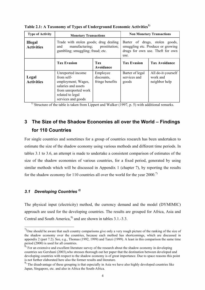
In table 3.2 the results for Asia are shown, recognizing that it is somewhat difficult to treat all
Asian countries equally because Japan, Singapore and Hongkong are highly developed
countries and the others more or less developing countries.
Table 3.2
If we consider these 26 Asian countries10), where the results are shown in table 3, Thailand
has by far the largest shadow economy in the year 2000 with the size of 52.6% of official
GDP; followed by Sri Lanka (44.6%) and the Philippines (43.4%). In the middle range are
India with an estimated shadow economy of 23.1% of official GDP, Israel with 21.9% and
Taiwan and China11) with 19.6%. At the lower end are Singapore (13.1%) and Japan (11.3%).
On average the Asian countries have a size of the shadow economy of 26% of official GDP
for the year 1999/2000. One realizes that the average size of the Asian shadow economies is
considerably lower compared with the ones of African and South and Latin American States –
partly due to the fact that in Asia we have a number of highly developed industrialized
countries with low shadow economies.
10) The case of India has been extensively investigated by Chatterjee, Chaudhury and Schneider (2003). 11) Here only parts of China are considered, which are converted into market economy.

6
Tabl
e 3.
1: T
he s
ize
of th
e sh
adow
and
offi
cial
eco
nom
y of
24
Afr
ican
nat
ions
A
FRIC
AN
nat
ion
GN
P at
mar
ket p
rices
(c
urre
nt U
S$, b
illio
n)
2000
Shad
ow E
cono
my
in
% o
f GN
P 19
99/2
000
Shad
ow E
cono
my
(cur
rent
USD
in
billi
on) 2
000
Shad
ow E
cono
my
GN
P pe
r cap
ita
(cur
rent
US$
)
GN
P pe
r cap
ita 2
000,
A
tlas
met
hod
(cur
rent
U
S$)
1 A
lger
ia
506,
1 34
,1
172,
6 53
8,8
1580
2 B
enin
21
,5
45,2
9,
7 16
7,2
370
3
Bot
swan
a 52
,8
33,4
17
,6
1102
,2
3300
4 B
urki
na F
aso
21,7
38
,4
8,3
80,6
21
0
5 C
amer
oon
82,8
32
,8
27,2
19
0,2
580
6
Cot
e d'
Ivoi
re
86,1
39
,9
34,4
23
9,4
600
7
Egyp
t, A
rab
Rep
.99
6,6
35,1
34
9,8
523,
0 14
90
8
Ethi
opia
63
,3
40,3
25
,5
40,3
10
0
9 G
hana
48
,3
38,4
18
,5
126,
7 33
0
10 K
enya
10
2,2
34,3
35
,1
120,
1 35
0
11 M
adag
asca
r 38
,0
39,6
15
,1
99,0
25
0
12 M
alaw
i 16
,6
40,3
6,
7 68
,5
170
13
Mal
i 22
,6
41,0
9,
3 98
,4
240
14
Mor
occo
32
4,6
36,4
11
8,1
429,
5 11
80
15
Moz
ambi
que
1)
35,8
40
,3
14,4
84
,6
210
16
Nig
er
18,1
41
,9
7,6
75,4
18
0
17 N
iger
ia
367,
3 57
,9
212,
6 15
0,5
260
18
Sen
egal
42
,9
43,2
18
,5
211,
7 49
0
19 S
outh
Afr
ica
1226
,4
28,4
34
8,3
857,
7 30
20
20
Tan
zani
a 89
,8
58,3
52
,4
157,
4 27
0
21 T
unis
ia
185,
7 38
,4
71,3
80
6,4
2100
22 U
gand
a 61
,6
43,1
26
,5
129,
3 30
0
23 Z
ambi
a 27
,9
48,9
13
,6
146,
7 30
0
24 Z
imba
bwe
1)
71,4
59
,4
42,4
27
3,2
460
A
VER
AG
E 18
8 41
69
28
0 76
4
1) D
ue to
civ
il w
ar a
nd p
oliti
cal u
nres
t unr
elia
ble
figur
es.
So
urce
: ow
n ca
lcul
atio
ns b
ased
on
Wor
ldba
nk D
ata,
Was
hing
ton
D.C
., 20
02.
7
Tabl
e 3.
2: T
he s
ize
of th
e sh
adow
and
offi
cial
eco
nom
y of
26
Asi
an c
ount
ries
A
SIA
G
NP
at m
arke
t pric
es
(cur
rent
US$
, bill
ion)
20
00
Shad
ow E
cono
my
in %
of G
NP
1999
/200
0
Shad
ow E
cono
my
(cur
rent
USD
in b
ill.)
2000
Shad
ow E
cono
my
GN
P pe
r cap
ita
(cur
rent
US$
)
GN
P pe
r cap
ita 2
000,
A
tlas
met
hod
(cur
rent
U
S$)
1 B
angl
ades
h 46
8,9
35,6
16
6,9
131,
7 37
0
2 C
hina
1)
1065
2,8
13,1
13
95,5
11
0,0
840
3
Hon
gkon
g, C
hina
1654
,7
16,6
27
4,7
4302
,7
2592
0
4 In
dia
4531
,8
23,1
10
46,8
10
4,0
450
5
Indo
nesi
a 2)
14
26,6
19
,4
276,
8 11
0,6
570
6
Iran
937,
7 18
,9
177,
2 30
4,3
1610
7 Is
rael
10
60,1
21
,9
232,
2 36
59,5
16
710
8
Japa
n 49
011,
6 11
,3
5538
,3
4025
,1
3562
0
9 Jo
rdan
83
,1
19,4
16
,1
331,
7 17
10
10
Kor
ea, R
ep.
4550
,2
27,5
12
51,3
24
50,3
89
10
11
Leb
anon
2)
174,
2 34
,1
59,4
13
67,4
40
10
12
Mal
aysi
a 82
3,9
31,1
25
6,2
1051
,2
3380
13 M
ongo
lia 1)
9,
5 18
,4
1,8
71,8
39
0
14 N
epal
56
,9
38,4
21
,8
92,2
24
0
15 P
akis
tan
596,
0 36
,8
219,
3 16
1,9
440
16
Phi
lippi
nes
793,
2 43
,4
344,
2 45
1,4
1040
17 S
audi
Ara
bia
1736
,6
18,4
31
9,5
1330
,3
7230
18 S
inga
pore
98
3,7
13,1
12
8,9
3240
,9
2474
0
19 S
ri La
nka
160,
0 44
,6
71,4
37
9,1
850
20
Syr
ia
159,
6 19
,3
30,8
18
1,4
940
21
Tai
wan
, Chi
na
3144
,0
19,6
61
6,2
2720
,5
1388
0
22 T
haila
nd
1205
,4
52,6
63
4,1
1052
,0
2000
23 T
urke
y 20
09,2
32
,1
644,
9 99
5,1
3100
24 U
nit.
Ara
b Em
ir.
0,0
26,4
0,
0 71
91,4
27
240
25
Vie
tnam
1)
313,
5 15
,6
48,9
60
,8
390
26
Yem
en
73,9
27
,4
20,2
10
1,4
370
A
VER
AG
E 33
31
26
531
1384
70
37
1)
Stil
l a m
ostly
com
mun
ist d
omin
ated
cou
ntry
. 2) D
ue to
civ
il w
ar a
nd p
oliti
cal u
nres
t unr
elia
ble
figur
es.
Sour
ce: o
wn
calc
ulat
ions
bas
ed o
n W
orld
bank
dat
a, W
ashi
ngto
n D
.C.,
2002
.

8
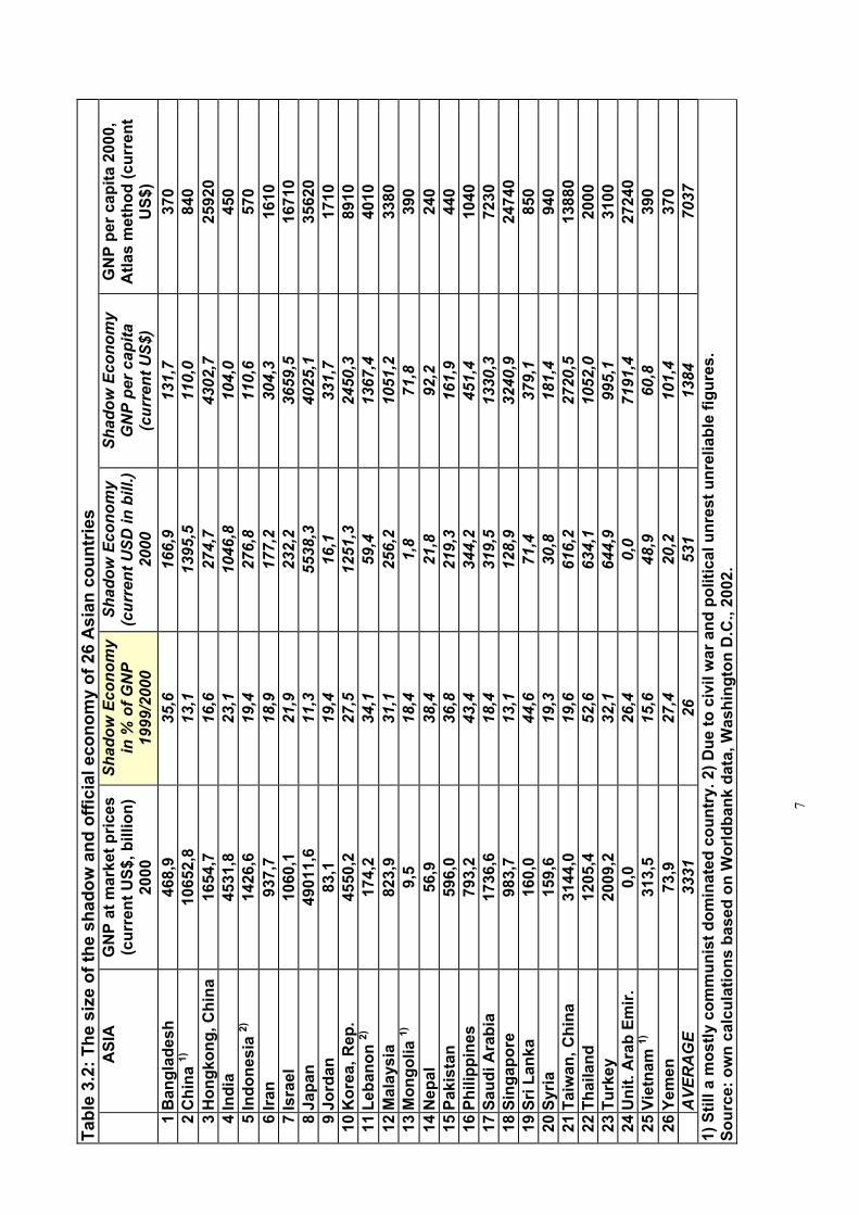
In table 3.3 the results of the sizes of the shadow economies for the year 2000 for 17 South
and Latin American countries are shown. The average size of shadow economy of these 17
countries is 41% of official GDP.
Table 3.3
The largest shadow economy is in Bolivia with 67.1%, followed by Panama (64.1%) and Peru
(59.9%). The smallest shadow economies are in Chile (19.8%) and Argentina (25.4%).
Overall the average sizes of the shadow economies of South and Latin America and of Africa
are generally similar and somewhat larger than in Asia – mostly due to the fact that in Asia
we have a number of highly industrialized and developed countries (Japan, Singapore, etc.).
3.2 Transition Countries
The measurement of the size and development of the shadow economy in the transition countries
has been undertaken since the late 80s starting with the work of Kaufmann and Kaliberda (1996),
Johnson et.al. (1997) and Lacko (2000). They all are using the physical input (electricity) method
(see Appendix 7.1.2.5) and come up with quite large figures. In the work of Alexeev and Pyle
(2003) the above mentioned studies are critically evaluated arguing that the estimated sizes of the
unofficial economies are to a large content a historical phenomenon only partly determined by
institutional factors.
In this paper the sizes of the shadow economies of the transition countries which have been
estimated the year 2000 using the DYMIMIC approach, are presented in table 3.4.
Table 3.4
23 transition countries have been investigated and the average size of the shadow economy
relative to official GDP is 38% for the year 1999/2000. Georgia has the by far largest shadow
economy at 67.3% of GDP, followed by Azerbaijan with 60.6% and Ukraine with 52.2%. In the
middle field are Bulgaria and Romania (36.9 and 34.4%, respectively) and at the lower end are
Hungary (25.1%), the Czech Republic (19.1%) and the Slowac. Republic (18.9%).
9
Tabl
e 3.
3: T
he s
ize
of th
e sh
adow
and
offi
cial
eco
nom
y of
17
Latin
and
Sou
th A
mer
ican
Cou
ntrie
s
SO
UTH
AM
ERIC
A
G
NP
at m
arke
t pric
es
(cur
rent
US$
, bill
ion)
20
00
Shad
ow
Econ
omy
in %
of
GN
P 19
99/2
000
Shad
ow E
cono
my
(cur
rent
USD
in
billi
on) 2
000
Shad
ow E
cono
my
GN
P pe
r cap
ita
(cur
rent
US$
)
GN
P pe
r cap
ita 2
000,
A
tlas
met
hod
(cur
rent
U
S$)
1 A
rgen
tina
27
74,4
25
,4
704,
7 18
94,8
74
60
2
Bol
ivia
80,6
67
,1
54,1
66
4,3
990
3
Bra
zil
56
97,7
39
,8
2267
,7
1424
,8
3580
4 C
hile
681,
4 19
,8
134,
9 90
8,8
4590
5 C
olom
bia
78
8,5
39,1
30
8,3
789,
8 20
20
6
Cos
ta R
ica
14
6,2
26,2
38
,3
998,
2 38
10
7
Dom
inic
an R
epub
lic
18
6,3
32,1
59
,8
683,
7 21
30
8
Ecua
dor
12
3,8
34,4
42
,6
416,
2 12
10
9
Gua
tem
ala
18
7,4
51,5
96
,5
865,
2 16
80
10
Hon
dura
s
57,9
49
,6
28,7
42
6,6
860
11
Jam
aica
69,9
36
,4
25,5
95
0,0
2610
12 M
exic
o
5597
,7
30,1
16
84,9
15
26,1
50
70
13
Nic
arag
ua
21
,1
45,2
9,
5 18
0,8
400
14
Pan
ama
93
,7
64,1
60
,1
2089
,7
3260
15 P
eru
51
9,2
59,9
31
1,0
1245
,9
2080
16 U
rugu
ay
19
3,8
51,1
99
,0
3066
,0
6000
17 V
enez
uela
, RB
1193
,2
33,6
40
0,9
1448
,2
4310
AVE
RA
GE
10
83
41
372
1152
30
62
So
urce
: ow
n ca
lcul
atio
ns b
ased
on
Wor
ldba
nk d
ata,
Was
hing
ton
D.C
., 20
02.

10
Tabl
e 3.
4: T
he s
ize
of th
e sh
adow
and
offi
cial
eco
nom
y of
23
Euro
pean
and
Asi
an T
rans
form
atio
n C
ount
ries
EU
RO
PE -
TRA
NSF
OR
MA
TIO
N
CO
UN
TRIE
S
G
NP
at m
arke
t pric
es
(cur
rent
US$
, bill
ion)
20
00
Shad
ow E
cono
my
in %
of G
NP
1999
/200
0
Shad
ow E
cono
my
(cur
rent
USD
in
billi
on) 2
000
Shad
ow E
cono
my
GN
P pe
r cap
ita
(cur
rent
US$
)
GN
P pe
r cap
ita 2
000,
Atla
s m
etho
d (c
urre
nt U
S$)
1 A
lban
ia 2)
38,6
33
,4
12,9
37
4,1
1120
2 A
rmen
ia
19
,3
46,3
8,
9 24
0,8
520
3
Aze
rbai
jan
1) 2
)
49,2
60
,6
29,8
36
3,6
600
4
Bel
arus
1)
29
9,6
48,1
14
4,1
1380
,5
2870
5 B
osni
a-H
erze
govi
na 2)
46,2
34
,1
15,8
41
9,4
1230
6 B
ulga
ria
11
6,7
36,9
43
,1
560,
9 15
20
7
Cro
atia
187,
2 33
,4
62,5
15
43,1
46
20
8
Cze
ch R
epub
lic
50
0,1
19,1
95
,5
1002
,8
5250
9 G
eorg
ia
30
,5
67,3
20
,5
424,
0 63
0
10 H
unga
ry
44
0,6
25,1
11
0,6
1182
,2
4710
11 K
azak
hsta
n 1)
170,
5 43
,2
73,7
54
4,3
1260
12 K
yrgy
z R
epub
lic
12
,2
39,8
4,
9 10
7,5
270
13
Lat
via
71
,8
39,9
28
,6
1165
,1
2920
14 L
ithua
nia
11
1,2
30,3
33
,7
887,
8 29
30
15
Mol
dova
1) 2
)
13,6
45
,1
6,1
180,
4 40
0
16 P
olan
d
1568
,2
27,6
43
2,8
1156
,4
4190
17 R
oman
ia
36
3,8
34,4
12
5,2
574,
5 16
70
18
Rus
sian
Fed
erat
ion 1
)
2484
,4
46,1
11
45,3
77
9,1
1690
19 S
lova
k R
epub
lic
18
7,7
18,9
35
,5
699,
3 37
00
20
Slo
veni
a
180,
7 27
,1
49,0
27
23,6
10
050
21
Ukr
aine
308,
5 52
,2
161,
0 36
5,4
700
22
Uzb
ekis
tan
1)
74
,2
34,1
25
,3
122,
8 36
0
23 Y
ugos
lavi
a 2)
84,5
29
,1
24,6
27
3,5
940
A
VER
AG
E
320
38
117
742
2354
1) S
till a
mos
tly c
omm
unis
t dom
inat
ed c
ount
ry. 2
) Due
to c
ivil
war
and
pol
itica
l unr
est u
nrel
iabl
e fig
ures
. So
urce
: ow
n ca
lcul
atio
ns b
ased
on
Wor
ldba
nk d
ata,
Was
hing
ton
D.C
., 20
02.

11
3.3 Highly developed OECD-Countries
OECD countries typically have a smaller shadow economy than the other country groupings. For
21 OECD countries the results are not only shown for the year 2000, but also over an extended
time period, i.e. from 1989 to 2002/2003; the results are presented in table 3.5.
Table 3.5
For the 21 OECD countries a combination of the currency demand method with the
DYMIMIC method is used.12) Considering again the latest period 2002/2003, Greece has with
28.3% of official GDP the largest shadow economy, followed by Italy with 26.2%13) and
Portugal with 22.3%. In the middle-field are Germany with a shadow economy of 16.8% of
official GDP, followed by Ireland with 15.5% and France with 14.8% of official GDP. At the
lower end are Austria with 10.8% of GDP and the United States with 8.6% of official GDP.
For these OECD countries one realizes over time a remarkable increase of the shadow
economies during the 90s. On average the shadow economy was 13.2% in these 21 OECD
states in the year 1989/90 and it rose to 16.4% in the year 2002/2003. If we consider the
second half of the 90s, we realize that for the majority of OECD countries the shadow
economy is not further increasing, even (slightly) decreasing, like for Belgium from 22.5%
(1997/98) to 21.5% (2002/2003), for Denmark from 18.3% (1997/98) to 17.5% (2002/2003)
or for Finland from 18.9% (1997/98) to 17.6% (2002/2003) or for Italy from 27.3% (1997/98)
to 26.2% (2002/2003). For others, like Austria, it is still increasing from 9.0% (1997/98) to
10.8% (2002/2003), or Germany from 14.9% (1997/98) to 16.8% (2002/2003). Hence, one
can’t draw a general conclusion whether the shadow economy is further increasing or
decreasing at the end of the 90s. It differs from country to country but in some countries some
efforts have been made to stabilize the size of the shadow economy and in other countries
(like Germany) these efforts were not successful up to the year 2003.
12) The case of Australia has been extensively investigated by Bajada (2002) and Bajada and Schneider (2003). 13) An extensive study of the size of the shadow economy of Italy was done by Dell’Anno (2003) and Dell’Anno and Schneider (2003), who achieve a similar but somewhat lower magnitude of the Italian shadow economy.

12
Table 3.5: The Size of the Shadow Economy in OECD Countries
Size of the Shadow Economy (in % of GDP) using the Currency Demand and DYMIMIC Method
OECD-Countries Average 1989/90
Average 1994/95
Average 1997/98
Average 1999/2000
Average 2001/2002
Average 2002/20031)
1. Australia 10.1 13.5 14.0 14.3 14.1 13.8
2. Belgium 19.3 21.5 22.5 22.2 22.0 21.5
3. Canada 12.8 14.8 16.2 16.0 15.8 15.4
4. Denmark 10.8 17.8 18.3 18.0 17.9 17.5
5. Germany 11.8 13.5 14.9 16.0 16.3 16.8
6. Finland 13.4 18.2 18.9 18.1 18.0 17.6
7. France 9.0 14.5 14.9 15.2 15.0 14.8
8. Greece 22.6 28.6 29.0 28.7 28.5 28.3
9. Great Britain 9.6 12.5 13.0 12.7 12.5 12.3
10. Ireland 11.0 15.4 16.2 15.9 15.7 15.5
11. Italy 22.8 26.0 27.3 27.1 27.0 26.2
12. Japan 8.8 10.6 11.1 11.2 11.1 11.0
13. Netherlands 11.9 13.7 13.5 13.1 13.0 12.8
14. New Zealand2) 9.2 11.3 11.9 12.8 12.6 12.4
15. Norweay 14.8 18.2 19.6 19.1 19.0 18.7
16. Austria 6.9 8.6 9.0 9.8 10.6 10.8
17. Portugal 15.9 22.1 23.1 22.7 22.5 22.3
18. Sweden 15.8 19.5 19.9 19.2 19.1 18.7
19. Switzerland 6.7 7.8 8.1 8.6 9.4 9.5
20. Spain 3) 16.1 22.4 23.1 22.7 22.5 22.3
21. USA 6.7 8.8 8.9 8.7 8.7 8.6
Unweighted Average over 21 OECD countries
13.2 15.7 16.7 16.8 16.7 16.4
Sources: Currency demand and DYMIMIC approach, own calculations 1) Preliminary values. 2) The figures are calculated using the MIMIC-method and Currency demand approach. Source: Giles (1999b). 3) The figures have been calculated for 1989/90, 1990/93 and 1994/95 from Mauleon (1998) and for the later periods own calculations.
3.4 Shadow Economy Labor Market
Having examined the size and development of the shadow economy in terms of value added
over time so far, the analysis now focuses on the „shadow“ labor market, as within the

13
official labor market there is a particularly tight relationship and “social network” between
people who are active in the shadow economy.14) Moreover, by definition every activity in the
shadow economy involves a “shadow” labor market to some extent: Hence, the “shadow
labor market” includes all cases, where the employees or the employers, or both, occupy a
„shadow economy position“.15) Illicit or shadow economy work can take many shapes. The
underground use of labor may consist of a second job after (or even during) regular working
hours. A second form is shadow economy work by individuals who do not participate in the
official labor market. A third component is the employment of people (e.g. clandestine or
illegal immigrants), who are not allowed to work in the official economy. Empirical research
on the shadow economy labor market is even more difficult than of the shadow economy on
the value added, since one has very little knowledge about how many hours an average
“shadow economy worker” is actually working (from full time to a few hours, only); hence, it
is not easy to provide empirical facts.16)
In table 3.6 the estimates for the shadow economy labor force of 7 OECD-countries (Austria,
Denmark, France, Germany, Italy, Spain and Sweden) are shown.
Table 3.6
In Austria the shadow economy labor force has reached in the years 1997-1998 500.000 to
750.000 or 16% of the official labor force (mean value). In Denmark the development of the
80s and 90s shows that the part of the Danish population engaged in the shadow economy
ranged from 8.3% of the total labor force (in 1980) to 15.4% in 1994 – quite a remarkable
increase of the shadow economy labor force; it almost doubled over 15 years. In France (in
the years 1997/98) the shadow economy labor force reached a size of between 6 and 12% of
the official labor force or in absolute figures between 1.4 and 3.2 million. In Germany this
figure rose from 8 to 12% in 1974 to 1982 and to 22% (18 millions) in the year 1997/98. This
is again a very strong increase in the shadow economy labor force for France and Germany.
For other countries the amount of the shadow economy labor force is quite large, too: in Italy
30-48% (1997-1998), Spain 11.5-32% (1997-1998) and Sweden 19.8 % (1997-1998). In the
14)Pioneering work in this area has been done by L. Frey (1972, 1975, 1978, 1980), Cappiello (1986), Lubell (1991), Pozo (1996), Bartlett (1998) and Tanzi (1999). 15) More detailed theoretical information on the labor supply decision in the underground economy is given by Lemieux, Fortin, and Fréchette (1994, p.235) who use micro data from a survey conducted in Quebec City (Canada). Their empirical findings clearly indicate, that “participation rates and hours worked in the underground sector also tend to be inversely related to the number of hours worked in the regular sector“. 16)For developing countries some literature about the shadow labour market exists, e.g. the latest works by Pozo (1996), Loayza (1996), especially Chickering and Salahdine (1991).

14
European Union about 30 million people are engaged in shadow economy activities in the
year 1997-1998 and in all European OECD-countries 48 million work illicitly.
Finally, in table 3.6 a first and preliminary calculation of the official GNP per capita and the
shadow economy GDP (working population) per capita is done, shown in US-$. Here one
realizes immediately that in all countries investigated, the shadow economy GDP per capita is
much higher - on average in all countries around 30%.17) In general these very preliminary
results clearly demonstrate that the shadow economy labor force has reached a remarkable
size in the developed OECD-countries, too, even when the calculation still might have many
errors.
4 The Main Causes of Determining the Shadow Economy
4.1 Tax and Social Security Contribution Burdens In almost all studies18) it has been found out, that the tax and social security contribution
burdens are one of the main causes for the existence of the shadow economy. Since taxes
affect labor-leisure choices, and also stimulate labor supply in the shadow economy, the
distortion of the overall tax burden is a major concern of economists. The bigger the
difference between the total cost of labor in the official economy and the after-tax earnings
(from work), the greater is the incentive to avoid this difference and to work in the shadow
economy. Since this difference depends broadly on the social security burden/payments and
the overall tax burden, they are key features of the existence and the increase of the shadow
economy.
But even major tax reforms with major tax rate deductions will not lead to a substantial
decrease of the shadow economy.19)
17) This is an astonishing result, which has to be further checked, because in the official per capita GDP figures the whole economy is included with quite productive sectors (like electronics, steel, machinery, etc.) and the shadow economy figures traditionally contain mostly the service sectors (and the construction sector). Hence one could also expect exactly the opposite result, as the productivity in the service sector is usually much lower than in the above mentioned ones. Sources of error may be either an underestimation of the shadow economy labor force or an overestimation of the shadow economy in terms of value added. 18) See Thomas (1992); Lippert and Walker (1997); Schneider (1994, 1997, 1998, 2000, 2003b); Johnson, Kaufmann, and Zoido-Lobatón (1998a,1998b); Tanzi (1999); Giles (1999a); Mummert and Schneider (2001); Giles and Tedds (2002) and Dell’Anno (2003), just to quote a few recent ones. 19)See Schneider (1994b, 1998b) for a similar result of the effects of a major tax reform in Austria on the shadow economy. Schneider shows that a major reduction in the direct tax burden did not lead to a major reduction in the shadow economy. Because legal tax avoidance was abolished and other factors, like regulations, were not changed; hence for a considerable part of the tax payers the actual tax and regulation burden remained unchanged.

15
Tab
le 3
.6: E
stim
ates
of t
he S
ize
of th
e “S
hado
w E
cono
my
Lab
or F
orce
” an
d of
the
Off
icia
l and
Sha
dow
Eco
nom
y pe
r ca
pita
197
4-19
98
Cou
ntri
es
Yea
r
Off
icia
l GD
P pe
r ca
pita
in
US-
$1)
Shad
ow
Eco
nom
y G
DP
in U
S-$
per
capi
ta
Size
of t
he
Shad
ow E
cono
my
(in %
of o
ffic
ial
GD
P) C
urre
ncy
Dem
and
App
roac
h2)
Shad
ow
Eco
nom
y L
abor
For
ce in
10
00 p
eopl
e3)
Shad
ow
Eco
nom
y Pa
rtic
ipan
ts in
%
of o
ffic
ial
Lab
or F
orce
4)
Sour
ces o
f Sha
dow
Eco
nom
y L
abou
r Fo
rce
Aus
tria
90
-91
97-9
8 20
,636
25
,874
25
,382
29
,630
5.
47
8.93
30
0-38
0 50
0-75
0 9.
6 16
.0
Schn
eide
r (1
998)
and
ow
n ca
lcul
atio
ns
Den
mar
k 19
80
13,2
33
18,6
58
8.6
250
8.3
Mog
ense
n, e
t. al
. (19
95)
19
94
34,4
41
48,5
62
17.6
42
0 15
.4
and
own
calc
ulat
ions
Fr
ance
19
75-8
2 19
97-9
8 12
,539
24
,363
17
,542
34
,379
6.
9 14
.9
800-
1500
14
00-3
200
3.0-
6.0
6.0-
12.0
D
e G
razi
a (1
983)
and
ow
n ca
lcul
atio
ns
Ger
man
y 19
74-8
2 19
97-9
8 11
,940
26
,080
17
,911
39
,634
10
.6
14.7
30
00-4
000
7000
-900
0 8.
0-12
.0
19.0
-23.
0 D
e G
razi
a (1
983)
, F. S
chne
ider
(199
8b)
and
own
calc
ulat
ions
It
aly
1979
19
97-9
8 8,
040
20,3
61
11,7
36
29,4
25
16.7
27
.3
4000
-700
0 66
00-1
1400
20
.0-3
5.0
30.0
-48.
0 G
aeta
ni a
nd d
’Ara
gona
(197
9) a
nd
ow
n ca
lcul
atio
ns
Spai
n 19
79-8
0 19
97-9
8 5,
640
13,7
91
7,86
8 19
,927
19
.0
23.1
12
50-3
500
1500
-420
0 9.
6-26
.5
11.5
-32.
3 R
uesg
a (1
984)
and
ow
n ca
lcul
atio
ns
Swed
en
1978
19
97-9
8 15
,107
25
,685
21
,981
37
,331
13
.0
19.8
75
0 11
50
13.0
-14.
0 19
.8
De
Gra
zia
(198
3) a
nd o
wn
calc
ulat
ions
Euro
pean
U
nion
19
78
1997
-98
9,93
0 22
,179
14
,458
32
,226
14
.5
19.6
15
000
30
000
-
De
Gra
zia (1
983)
and
own
cal
cula
tions
OEC
D
(Eur
ope)
19
78
1997
-98
9,57
6 22
,880
14
,162
33
,176
15
.0
20.2
26
000
48
000
-
De
Gra
zia (1
983)
and
own
cal
cula
tions
1) S
ourc
e: O
ECD
, Par
is, v
ario
us y
ears
2)
Sou
rce:
Ow
n ca
lcul
atio
ns.
3) E
stim
ated
full-
time
jobs
, inc
ludi
ng u
nreg
iste
red
wor
kers
, ille
gal i
mm
igra
nts,
and
seco
nd jo
bs.
4) In
per
cent
of t
he p
opul
atio
n ag
ed 2
0-69
, sur
vey
met
hod.

16
Such reforms will only be able to stabilize the size of the shadow economy and avoid a further
increase. Social networks and personal relationships, the high profit from irregular activities
and associated investments in real and human capital are strong ties which prevent people
from transferring to the official economy. For Canada, Spiro (1993) found similar reactions of
people facing an increase in indirect taxes (VAT, GST). This fact makes it even more difficult
for politicians to carry out major reforms because they may not gain a lot from them.
The most important factor in neoclassical models is the marginal tax rate. The higher the
marginal tax rate, the greater is the substitution effect and the bigger the distortion of the
labor-leisure decision. Especially when taking into account that the individual can also receive
income in the shadow economy, the substitution effect is definitely larger than the income
effect and, hence, the individual works less in the official sector. The overall efficiency of the
economy is, therefore (ceteris paribus), lower and the distortion leads to a welfare loss
(according to official GNP and taxation.) But according to Thomas (1992, p.134) the welfare
might also be viewed as increasing, if the welfare of those, who are working in the shadow
economy, were taken into account, too.
Empirical results of the influence of the tax burden on the shadow economy is provided in the
studies of Schneider (1994b, 2000) and Johnson, Kaufmann and Zoido-Lobatón (1998a,
1998b); they all found statistically significant evidence for the influence of taxation on the
shadow economy. This strong influence of indirect and direct taxation on the shadow
economy will be further demonstrated by discussing empirical results in the case of Austria
and the Scandinavian countries. For Austria the driving force for the shadow economy
activities is the direct tax burden (including social security payments), it has the biggest
influence, followed by the intensity of regulation and complexity of the tax system. A similar
result has been achieved by Schneider (1986) for the Scandinavian countries (Denmark,
Norway and Sweden). In all three countries various tax variables (average direct tax rate,
average total tax rate (indirect and direct tax rate)) and marginal tax rates have the expected
positive sign (on currency demand) and are highly statistically significant. These findings are
supported by studies of Kirchgaessner (1983, 1984) for Germany and by Kloveland (1984) for
Norway and Sweden, too.
Several other recent studies provide further evidence of the influence of income tax rates on
the shadow economy: Cebula (1997), using Feige data for the shadow economy, found
evidence of the impact of income tax rates, IRS audit probabilities, and IRS penalty policies
on the relative size of the shadow economy in the United States. Cebula concludes that a

17
restraint of any further increase of the top marginal income tax rate may at least not lead to a
further increase of the shadow economy, while increased IRS audits and penalties might
reduce the size of the shadow economy. For example, if the marginal federal personal income
tax rate increases by one percentage point, ceteris paribus, the shadow economy rises by 1.4
percentage points. In another investigation, Hill and Kabir (1996) found empirical evidence
that marginal tax rates are more relevant than average tax rates, and that a substitution of
direct taxes by indirect taxes seems unlikely to improve tax compliance. Further evidence on
the effect of taxation on the shadow economy is presented by Johnson, Kaufmann, and Zoido-
Lobatón (1998b), who come to the conclusion that it is not higher tax rates per se that
increase the size of the shadow economy, but the ineffective and discretionary application of
the tax system and the regulations by governments. In their study they find a positive
correlation between the size of the shadow economy and the corporate tax burden. They come
to the overall conclusion that there is a large difference between the impact of either direct
taxes or the corporate tax burden. Institutional aspects, like the efficiency of the
administration, the extent of control rights held by politicians and bureaucrats, and the amount
of bribery and especially corruption, therefore, play a major role in this “bargaining game“
between the government and the taxpayers.
4.2 Intensity of Regulations The increase of the intensity of regulations (often measured in the numbers of laws and
regulations, like licenses requirements) is another important factor, which reduces the
freedom (of choice) for individuals engaged in the official economy.20) One can think of labor
market regulations, trade barriers, and labor restrictions for foreigners. Johnson, Kaufmann,
and Zoido-Lobatón (1998b) find an overall significant empirical evidence of the influence of
(labor) regulations on the shadow economy, the impact is clearly described and theoretically
derived in other studies, e.g. for Germany (Deregulation Commission 1990/91). Regulations
lead to a substantial increase in labor costs in the official economy. But since most of these
costs can be shifted on the employees, these costs provide another incentive to work in the
shadow economy, where they can be avoided. Empirical evidence supporting the model of
Johnson, Kaufmann, and Shleifer (1997), which predicts, inter alia, that countries with more
general regulation of their economies tend to have a higher share of the unofficial economy in
total GDP, is found in their empirical analysis. A one-point increase of the regulation index 20)See for a (social) psychological, theoretical foundation of this feature, Brehm (1966, 1972), and for a (first)

18
(ranging from 1 to 5, with 5 = the most regulation in a country), ceteris paribus, is associated
with an 8.1 percentage point increase in the share of the shadow economy, when controlled
for GDP per capita (Johnson et. al. (1998b), p. 18). They conclude that it is the enforcement
of regulation, which is the key factor for the burden levied on firms and individuals, and not
the overall extent of regulation - mostly not enforced - which drive firms into the shadow
economy. Friedman, Johnson, Kaufmann and Zoido-Lobaton (1999) reach a similar result. In
their study every available measure of regulation is significantly correlated with the share of
the unofficial economy and the sign of the relationship is unambiguous: more regulation is
correlated with a larger shadow economy. A one point increase in an index of regulation
(ranging from 1-5) is associated with a 10 % increase in the shadow economy for 76
developing, transition and developed countries.
These findings demonstrate that governments should put more emphasis on improving
enforcement of laws and regulations, rather than increasing their number. Some governments,
however, prefer this policy option (more regulations and laws), when trying to reduce the
shadow economy, mostly because it leads to an increase in power of the bureaucrats and to a
higher rate of employment in the public sector.
4.3 Public Sector Services
An increase of the shadow economy can lead to reduced state revenues which in turn reduce
the quality and quantity of publicly provided goods and services. Ultimately, this can lead to
an increase in the tax rates for firms and individuals in the official sector, quite often
combined with a deterioration in the quality of the public goods (such as the public
infrastructure) and of the administration, with the consequence of even stronger incentives to
participate in the shadow economy. Johnson, Kaufmann, and Zoido-Lobatón (1998a,b)
present a simple model of this relationship. Their findings show that smaller shadow
economies appear in countries with higher tax revenues, if achieved by lower tax rates, fewer
laws and regulations and less bribery facing enterprises. Countries with a better rule of the
law, which is financed by tax revenues, also have smaller shadow economies. Transition
countries have higher levels of regulation leading to a significantly higher incidence of
bribery, higher effective taxes on official activities and a large discretionary framework of
regulations and consequently to a higher shadow economy. Their overall conclusion is that
“wealthier countries of the OECD, as well as some in Eastern Europe find themselves in the
application to the shadow economy, Pelzmann (1988).

19
‘good equilibrium’ of relatively low tax and regulatory burden, sizeable revenue mobilization,
good rule of law and corruption control, and [relatively] small unofficial economy. By
contrast, a number of countries in Latin American and the Former Soviet Union exhibit
characteristics consistent with a ‘bad equilibrium’: tax and regulatory discretion and burden
on the firm is high, the rule of law is weak, and there is a high incidence of bribery and a
relatively high share of activities in the unofficial economy.“ (Johnson, Kaufmann and Zoido-
Lobatón 1998a p. I).
5 The Dynamic Effects of the Shadow Economy on Official Economy
5.1 Theoretical Background
Generally, the view prevails that the informal sector/the shadow economy influences the tax
system and its structure, the efficiency of resource allocation between sectors, and the official
economy as a whole in a dynamic sense. In order to study the effects of the shadow economy
on the official one, several studies integrate underground economies into theoretical or
empirical macroeconomic models.21 For example, Houston (1987) develops a theoretical
business cycle model, in which there are tax and monetary policy linkages with the shadow
economy, and concludes that the existence of a shadow economy could lead to an
overstatement of the inflationary effects of fiscal or monetary stimulus. In an empirical study
for Belgium Adam and Ginsburgh (1985) focus on the implications of the shadow economy
on "official" growth and find a positive relationship between the growth of the shadow
economy and the "official" one and under certain assumptions (i.e. very low entry costs into
the shadow economy due to a low probability of enforcement). They conclude that an
expansionary fiscal policy is a positive stimulus for both the formal and informal economies.
Another hypothesis is, that a substantial reduction of the shadow economy leads to a
significant increase in tax revenues and therefore to a greater quantity and quality of public
goods and services, which ultimately can stimulate economic growth. Some authors found
empirical evidence for this hypothesis. Loayza (1996) presents a simple macroeconomic
endogenous growth model in which production technology depends on congestable public
services and in which “excessive” taxes and regulations are imposed by governments unable
to enforce fully compliance. He concludes that an increase in the relative size of the informal 21 For Austria this was done by Schneider, Hofreither, and Neck (1989) and Neck, Hofreither, and Schneider

20
economy reduces economic growth in economies where (1) the statutory tax burden is larger
than the optimal tax burden and where (2) the enforcement of compliance is weak. The reason
for this negative correlation is the strongly negative correlation between the informal sector
and public infrastructure indices, while public-infrastructure is the key element for economic
growth. Loayza (1996) also finds empirical evidence for Latin America countries that if the
shadow economy increases by one percentage point (of GDP) - ceteris paribus - the growth
rate of official real GDP per capita decreases by 1.22 percentage points. However, this
negative impact of informal sector activities on economic growth is not broadly accepted, e.g.
by Asea (1996). For example, the Loayza (1996) model is based on the assumption that the
production technology depends on tax-financed public services, that are subject to congestion
and that the informal sector is not paying any taxes but must pay penalties that are not used to
finance public services. The negative correlation between the size of the informal sector and
economic growth is therefore not very surprising.
Further, in the neoclassical view the underground economy is optimal in the sense that it
responds to the economic environment's demand for urban services and small-scale
manufacturing. From this point of view the informal sector provides the economy with a
dynamic and entrepreneurial spirit and can lead to more competition, higher efficiency, and
stronger boundaries and limits for government activities. Put it differently, the informal sector
may help to create markets, increase financial resources, enhance entrepreneurship, and
transform the legal, social, and economic institutions necessary for accumulation“ (Asea,
1996 p. 166). The voluntary self-selection between the formal and informal sectors may
provide a higher potential for economic growth and hence a positive correlation between an
increase of the informal sector and economic growth. Finally, considering both lines of
theoretical argumentation, the effects of an increase of the shadow economy on economic
growth therefore remain considerably ambiguous. It may be that on the one side in highly
developed countries people/entrepreneurs are overburdened by tax and regulation so that a
rising shadow economy stimulates/increases the official one as additional value added is
created and additional income earned in the shadow economy is spent in the official one. On
the other side in developing countries a rising shadow economy leads to a considerable
erosion of the tax base with the consequence of a lower provision of public infrastructure and
basic public service (e.g. an efficient juridical system) and with the final consequence of
lower official growth.
(1989). For further discussion of this aspect see Quirk (1996) and Giles (1999a).

21
Accordingly, we test empirically the impact of the size of the shadow economy upon
“official” economic growth. We construct a panel data set for 109 developing, transition, and
OECD countries for the time period from 1990 to 2000 to estimate the possible effects of the
shadow economy on the official one.
Our panel data set consists of variables22 that the growth theory suggests to be relevant for
economic growth [Barro et al. 1995 and Breton 2001]. The data set includes such explanatory
variables as the size of the shadow economy (as percent of “official” GDP), capital
accumulation, labour force and population growth rates, inflation rates, an indicator for
openness, figures on foreign direct investment, the corruption index, government expenditures
and GDP per capita [to control for the convergence hypothesis23] in order to estimate the
relationship between economic growth, the shadow economy, and other possible factors.
5.2 The Main Results
We estimate a basic equation for the entire sample of 109 developing and developed countries
and variables on this basic equation for the two separate sub-samples of 21 OECD countries
and 75 developing and transition countries. In all regressions, the dependent variable is the
average applied growth rate in per capita GDP over the 1990 to 2000 period. Appendix 2 (7.2)
contains a description of the countries and our variables.
5.2.1 The Sample of 109 Developing and Developed Countries Our empirical estimation equation is the following:
“official” economic growth = a1 (shadow economy industrialized countries) +
a2 (shadow economy developing countries) +
a3 (openness) +
a4 (inflation rate industrialized countries) +
a5 (inflation rate developed countries) +
a6 (government consumption) +
a7 (lagged GDP per capita growth rate) +
a8 (total population) +
a9 (capital accumulation rate) +
a10 (constant) + εit 22 A description of the countries, variables and sources can be found more detailed in the part 7.2, Appendix at the end of this paper. 23 The convergence theory argues that countries with a lower GDP per capita should have higher annual GDP

22
with the expected signs = a1 > 0, a2 < 0, a3 > 0, a4 < 0, a5 < 0, a6 < 0, a7 > 0, a8 > 0, a9 > 0
Not all of the theoretically relevant variables for economic growth just like expenditures on
research and development [R&D] as an indicator for technological progress or indicators for
human capital like school enrollment and number of persons with secondary and tertiary
education were available24 for all 109 countries for the regression analysis but the dataset is
quite adequate for testing the dynamic influence of the shadow economy on the official one.
Putting all possible (for all countries available) variables into an equation explaining
economic growth did not deliver satisfying results, since many conventionally important
variables were insignificant. For example labour force growth has no influence on the GDP
growth rate in the model despite the fact that theory suggests a positive relationship between
labour force growth and economic growth [Breton 2001]; similarly, neither the corruption
index ranging from 0 to 1025 nor foreign direct investment had a statistically significant
impact on annual GDP growth.
Accordingly, we followed a ‘testing down procedure’26 to address possible misspecification.
After testing different model specifications the following model, reported in table 5.1,
resulted, which is “our best” model.
growth rates since they are following a catching up process. 24 Some variables were not available at all but most variables were available only for a small number of countries and many observations would have been lost if using the particular variable in the regression analysis [for example using patents per year as a proxy variable for expenditures on R&D results in a sample consisting only of 30 countries]. The 109 countries are listed in the appendix 2 (part 7.2). 25 The higher the value of the corruption index, the lower corruption in the observed country. 26 The ‘testing down procedure’ means that step by step insignificant variables are dropped from the equation after carrying out F-tests on joint significance [see Wooldridge 2000, page 139 - 150]. For example the coefficient on GDP per capita was insignificant and the convergence theory cannot be supported with the available data.

23
Table 5.1.: Results of the Panel Regression; Time period 1990 – 2000, 104 developing, transition and industrialized countries
Dependent Variable Annual GDP per capita Growth Rate
Independent Variables: Estimated Coefficients: Shadow Economy Industrialized Countries 0.077** (2.63) Shadow Economy Developing Countries -0.052** (2.37) Openness 0.012** (2.14) Inflation Rate Other Countries 0.023 (1.32) Inflation Rate Transition Countries -0.021** (4.10) Government Consumption -0.181** (3.23) Lagged Annual GDP per capita Growth Rate 0.154** (3.06) Total Population 0.000036** (2.07) Capital Accumulation Rate 0.019* (1.88) Constant 0.062** (4.13) Number of countries 104 Overall R-Squared 0.347 Within R-Squared 0.266 Between R-Squared 0.417 Wald-CHI² 94.63 (0.000) Absolute value of z-statistics in parentheses * significant at 10%; ** significant at 5%. Random effects GLS-regressions; 104 countries, period 1990-2000; yearly data Source: Own Calculation by authors
This regression clearly shows a highly interesting and statistically significant negative
relationship between the shadow economy of developing countries and official rate of
economic growth and a statistically significant positive relationship between the shadow
economy in industrialized countries and economic growth. If the shadow economy in
industrialized countries raises by 1 percentage point of GDP (e.g. shadow economy increases
from 10 of 11 percent of official GDP) official growth increases by 7.7 percent; in contrast,
for developing countries an increase of the shadow economy by 1 percentage point of official
GDP is associated with a decrease in the official growth rate by 4.9 percent. Also all other
variables (except the inflation rate in other countries) have a statistically significant influence
on growth. For example, the more open a country the higher is official growth and if the
24
inflation rate in transition countries increases by 1 percent official growth decreases by 2.1
percent. Similarly, an increase in the state sector by 1 percent is a associated with a decreases
in growth by 1.8 percent. On the other hand, an increase in the total population by 10 million
leads to an increase in official GDP by 0.36 percent.
In general these results clearly show a statistically significant negative impact of the shadow
economy of developing countries on the growth rate of the official economy and a positive
influence of the shadow economy on the growth rate of industrialized countries. All other
variables have plausible signs and are generally statistically significant on a 5 percent
confidence level
5.2.2 21 OECD countries When we focus more narrowly on OECD countries, we find similar results. The 21 OECD
countries are Australia, Belgium, Canada, Denmark, Germany, Finland, France, Greece, Great
Britain, Ireland, Italy, Japan, Netherlands, New Zealand, Norway, Austria, Portugal, Sweden,
Switzerland, Spain, and the USA. As before we estimate a panel regression with the official
growth rate of GDP per capita of the 1990 up to 2000 period as dependent variable.
For these 21 OECD countries we specify the following growth equation:
“official” growth (annual GDP per capita) = a1 (trendvariable) +
a2 (shadow economy) +
a3 (openness) +
a4 (capital accumulation rate) +
a5 (annual FDY growth rate) +
a6 (annual labour force growth rate) +
a7 (constant) + εit
For the signs we expect a1 > 0, a2 > 0, a3 > 0, a4 > 0, a5 > 0.

25
Table 5.2.: Growth equation for 21 OECD Countries 1990 – 2000; results of a Panel regression
Dependent Variables Annual GDP per capita Growth Rate
Explanatory Variables: Estimated coefficients Trend Variable -0.003** (3.36) Shadow Economy 0.078** (2.05) Openness 0.016** (2.47) Capital Accumulation Rate 0.127** (3.47) Annual FDI Growth Rate 0.004** (2.49) Annual Labour Force Growth Rate 0.951** (2.44) Constant 6.206** (3.36) Number of countries 21 Overall R-Squared 0.370 Within R-Squared 0.213 Between R-Squared 0.716 Wald-Chi² 51.10 (0.000) Absolute value of z-statistics in parentheses * significant at 10%; ** significant at 5%; Random effects GLS-regressions; 21 countries, period 1990-2000; yearly data Source: Own Calculation by authors
The empirical estimation results are shown in table 5.2. The trend variable clearly has a
negative and a statistically significant influence on the official growth rate in the OECD
countries – a result which is not unusual for the period of the 90s for most OECD countries,
as it reflects the overall poor economic performance of most OECD countries during the 90s.
Again, the shadow economy has a positive and a statistically significant influence on the
official growth rate of GDP per capita. An increase in the shadow economy by 1 percentage
point (of official GDP) is associated with an increase in the annual growth rate of 7.8 percent.
In addition, increases in the capital accumulation rate by 1 percentage point, lead to an official
growth by 12.7 percent. If foreign direct investment increases by 1 percentage point, annual
growth rate increases by 0.4 percent. If the annual labor force rate increases by 1 percent,
growth rate increases by 9.5 percent.

26
5.2.3 75 Transition and Developing Countries Official economy growth of highly industrialized, developing and transition countries may be
quite different then that of developed and transition countries and the explanatory factors that
influence the growth rate may also be quite different (due to institutional reasons), we finally
present an estimation with only developing and transition countries. For these 75 countries we
specify the following growth equation:
“Official” growth (annual GDP per capita) = a1 (shadow economy transition countries) +
a2 (shadow economy developing countries) +
a3 (foreign direct investment lagged) +
a4 (inflation rate other countries) +
a5 (inflation rate transition countries) +
a6 (government consumption) +
a7 (lagged annual GDP per capita) +
a8 (growth rate) +
a9 (population rate) +
a10 (capital accumulation rate) +
a11 (constant) + εit
For the signs we expect: a1 > 0, a2 < 0, a3 > 0, a4 < 0, a5 < 0, a6 < 0, a7 > 0, a8 > 0, a9 > 0.
The empirical results are shown in table 5.3.
27
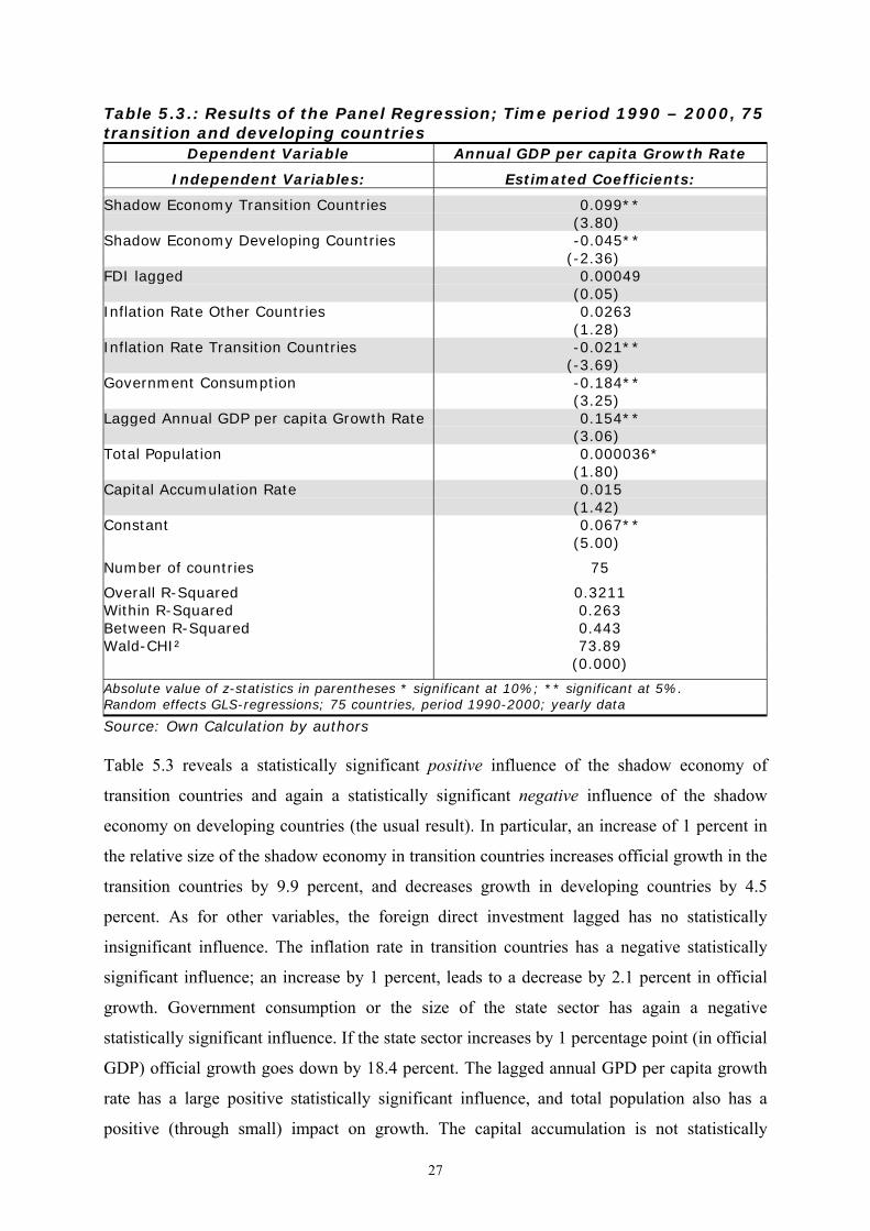
Table 5.3.: Results of the Panel Regression; Time period 1990 – 2000, 75 transition and developing countries
Dependent Variable Annual GDP per capita Growth Rate
Independent Variables: Estimated Coefficients:
Shadow Economy Transition Countries 0.099** (3.80) Shadow Economy Developing Countries -0.045** (-2.36) FDI lagged 0.00049 (0.05) Inflation Rate Other Countries 0.0263 (1.28) Inflation Rate Transition Countries -0.021** (-3.69) Government Consumption -0.184** (3.25) Lagged Annual GDP per capita Growth Rate 0.154** (3.06) Total Population 0.000036* (1.80) Capital Accumulation Rate 0.015 (1.42) Constant 0.067** (5.00)
Number of countries 75
Overall R-Squared 0.3211 Within R-Squared 0.263 Between R-Squared 0.443 Wald-CHI² 73.89 (0.000)
Absolute value of z-statistics in parentheses * significant at 10%; ** significant at 5%. Random effects GLS-regressions; 75 countries, period 1990-2000; yearly data
Source: Own Calculation by authors
Table 5.3 reveals a statistically significant positive influence of the shadow economy of
transition countries and again a statistically significant negative influence of the shadow
economy on developing countries (the usual result). In particular, an increase of 1 percent in
the relative size of the shadow economy in transition countries increases official growth in the
transition countries by 9.9 percent, and decreases growth in developing countries by 4.5
percent. As for other variables, the foreign direct investment lagged has no statistically
insignificant influence. The inflation rate in transition countries has a negative statistically
significant influence; an increase by 1 percent, leads to a decrease by 2.1 percent in official
growth. Government consumption or the size of the state sector has again a negative
statistically significant influence. If the state sector increases by 1 percentage point (in official
GDP) official growth goes down by 18.4 percent. The lagged annual GPD per capita growth
rate has a large positive statistically significant influence, and total population also has a
positive (through small) impact on growth. The capital accumulation is not statistically

28
significant.
In summary, all three sets of regression clearly indicate that the shadow economy has a
statistically significant influence on official economic growth. For transition countries and
highly industrialized (OECD) countries this influence is positive, while for developing
countries the shadow economy has a negative influence on official growth. These results (at
least partly) confirm our discussion of the theoretical considerations in part 5.1.
6 Summary and Conclusions
There are many obstacles to be overcome to measure the size of the shadow economy and to
analyze its consequences on the official economy, but as this paper shows some progress has
been made. We have been shown that though it is difficult to estimate the size of the shadow
economy. We provided estimates for 110 countries all over the world. We have demonstrated
that with various methods, e.g. the currency demand, and the model (MIMIC) approach, some
insights can be provided into the size and development of the shadow economy of the
developing, transition and the OECD countries. The general impression from the results of
these methods is that for all countries investigated the shadow economy has reached a
remarkably large size. The summarized results are shown in table 6.1.
Table 6.1: Average Size of the Shadow Economy for Developing, Transition and OECD-Countries in Terms of Value-Added for 2000
Average Size of the Shadow Economy – Value added in % of official GDP 2000
Countries Currency Demand and DYMIMIC method (Number of Countries)
Mostly developing countries: Africa 41
(23) Central and South America 41
(18) Asia 29
(26) Transition countries 35
(23) European OECD Countries 18
(16)
North American and Pacific OECD Countries
13.5 (4)
Source: Own calculations.

29
We have also demonstrated that there is an empirically strong interaction of the shadow
economy with the official one. From these two major results we draw the following four
conclusions:
(1) As it has already been argued, there is no „best“ or commonly accepted method; each
approach has its specific strengths and weaknesses as well as specific insights and
results. Although the different methods provide a rather wide range of estimates, there
is a common finding that the size of the shadow economies for developing, transition,
and OECD countries has been growing over the 1990 to 2000 period.
(2) Furthermore, the results of our study show that an increasing burden of taxation and
social security payments, combined with rising state regulatory activities, are the
major driving forces for the size and growth of the shadow economy.
(3) A further important result of our study is that the shadow economy has a statistically
significant and quantitatively important influence on the growth of the official
economy. If the shadow economy increases by one percentage point (shadow
economy in percent of official GDP) the official growth in a developing country
declines between 4.5 and 5.7 percent. For developed (industrialized and /or transition)
countries we find the opposite result. If the shadow economy increases by one
percentage point (in % of GDP) the growth rate in industrialized countries increases
by 7.7 percent and by 9.9 percent in transition countries, respectively.
(4) Finally, to conclude: Shadow economies are a complex phenomenon, present to an
important extent in all type of economies (developing, transition and developed).
People engage in shadow economic activity for a variety of reasons, among most
important, of which we can count are government actions, most notable taxation and
regulation. With these two insights, goes a third, no less important one: a government
aiming to decrease shadow economic activity has to first and foremost analyze the
complex and frequently contradictory relationships among consequences of its own
policy decisions.

30
7 Appendices
7.1 Appendix 1: Methods to Estimate the Size of the Shadow Economy
As has already been mentioned in chapters 2 and 3 to estimating the size of a shadow
economy is a difficult and challenging task. In this appendix we give a short but
comprehensive overview on the various procedures to estimate the size of a shadow economy.
Three different types of methods are most widely used, and each is briefly discussed.
7.1.1 Direct Approaches These are micro approaches that employ either well designed surveys and samples based on
voluntary replies or tax auditing and other compliance methods. Sample surveys designed to
estimate the shadow economy are widely used in a number of countries27). The main
disadvantage of this method is that it presents the flaws of all surveys. For example, the
average precision and results depend greatly on the respondent’s willingness to cooperate, it is
difficult to asses the amount of undeclared work from a direct questionnaire, most
interviewers hesitate to confess a fraudulent behavior, and responses are of uncertain
reliability, which makes it difficult to calculate a real estimate (in monetary terms) of the
extend of undeclared work. The main advantage of this method lies in the detailed
information about the structure of the shadow economy, but the results from these kinds of
surveys are very sensitive to the way the questionnaire is formulated28).
Estimates of the shadow economy can also be based on the discrepancy between income
declared for tax purposes and that measured by selective checks. Fiscal auditing programs
have been particularly effective in this regard. Since these programs are designed to measure
the amount of undeclared taxable income, they may also be used to calculate the shadow
economy.29) However, a number of difficulties beset this approach. First, using tax
compliance data are equivalent to using a (possibly biased) sample of the population. In
general, the selection of tax payers for tax audit is not random but based on properties of
27)The direct method of voluntary sample surveys has been extensively used for Norway by Isachsen, Klovland and Strom (1982), and Isachsen and Strom (1985). For Denmark this method is used by Mogensen (et. al., 1995) in which they report „estimates“ of the shadow economy of 2.7 percent of GDP for 1989, of 4.2 percent of GDP for 1991, of 3.0 percent of GDP for 1993 and of 3.1 percent of GDP for 1994. 28)The advantages and disadvantages of this method are extensively dealt by Mogensen et. al (1995) in their excellent and very carefully done investigation. 29)In the United States, IRS (1979, 1983), Simon and Witte (1982), Witte (1987), Clotefelter (1983), and Feige (1986). For a more detailed discussion, see Dallago (1990) and Thomas (1992).
31
submitted (tax) returns that indicate a certain likelihood of (tax) fraud. Consequently, such a
sample is not a random one of the whole population, and estimates of the shadow based upon
a biased sample may not be accurate. Second estimates based on tax audits reflect only that
portion of shadow economy income that the authorities succeed in discovering, and this is
likely to be only a fraction of hidden income.
A further disadvantage of these two direct methods (surveys and tax auditing) is that they lead
only to point estimates. Moreover, it is unlikely that they capture all „shadow“ activities, so
they can be seen as providing lower bound estimates. They are unable to provide estimates of
the development and growth of the shadow economy over a longer period of time. As already
argued, they have, however at least one considerable advantage - they can provide detailed
information about shadow economy activities and the structure and composition of those who
work in the shadow economy.
7.1.2 Indirect Approaches These approaches, which are also called „indicator“ approaches, are mostly macroeconomic
ones and use various economic and other indicators that contain information about the
development of the shadow economy (over time). Currently there are five indicators that
leave some „traces“ of the shadow economy.
7.1.2.1 The Discrepancy between National Expenditure and Income Statistics This approach is based on discrepancies between income and expenditure statistics. In
national accounting the income measure of GNP should be equal to the expenditure measure
of GNP. Thus, if an independent estimate of the expenditure site of the national accounts is
available, the gap between the expenditure measure and the income measure can be used as an
indicator of the extent of the black economy.30) Since national accounts statisticians are
anxious to minimize this discrepancy, the initial discrepancy or first estimate, rather than the
published discrepancy should be employed as an estimate of the shadow economy. If all the
components of the expenditure site are measured without error, then this approach would
indeed yield a good estimate of the scale of the shadow economy. Unfortunately, however,
this is not the case. Instead, the discrepancy reflects all omissions and errors everywhere in
30) See, e.g., Franz (1983) for Austria; MacAfee (1980) O’Higgins (1989) and Smith (1985), for Great Britain; Petersen (1982) and Del Boca (1981) for Germany; Park (1979) for the United States. For a critical survey, see Thomas (1992).

32
the national accounts statistics as well as the shadow economy activity. These estimates may
therefore be very crude and of questionable reliability.31)
7.1.2.2 The Discrepancy between the Official and Actual Labor Force A decline in participation of the labor force in the official economy can be seen as an
indication of increased activity in the shadow economy. If total labor force participation is
assumed to be constant, than a decreasing official rate of participation can be seen as an
indicator of an increase in the activities in the shadow economy, ceteris paribus.32) One
weakness of this method is that differences in the rate of participation may also have other
causes. Also, people can work in the shadow economy and have a job in the „official’
economy. Therefore such estimates may be viewed as weak indicators of the size and
development of the shadow economy.
7.1.2.3 The Transactions Approach This approach has been most fully developed by Feige.33) It is based upon the assumption,
that there is a constant relation over time between the volume of transaction and official GNP,
as summarized by the well-known Fisherian quantity equation, or M*V = p*T (with M =
money, V = velocity, p = prices, and T = total transactions). Assumptions also have to be
made about the velocity of money and about the relationships between the value of total
transactions (p*T) and total (=official + unofficial) nominal GNP. Relating total nominal
GNP to total transactions, the GNP of the shadow economy can be calculated by subtracting
the official GNP from total nominal GNP. However, to derive figures for the shadow
economy, one must also assume a base year in which there is no shadow economy and
therefore the ratio of p*T to total nominal (official = total) GNP was „normal“ and would
have been constant over time, if there had been no shadow economy.
This method, too, has several weaknesses, such as the required assumptions of a base year
with no shadow economy, and of a „normal“ ratio of transactions to nominal GNP. Moreover,
to obtain reliable shadow economy estimates, precise figures of the total volume of
transactions should be available, and this availability might be especially difficult to achieve
for cash transactions, because they depend, among other factors, on the durability of bank
notes in terms of the quality of the papers on which they are printed.34) Also, the assumption
31) A related approach is pursued by Pissarides and Weber (1988), who use micro data from household budget surveys to estimate the extend of income understatement by self-employed. 32) Such studies have been made for Italy, see e.g., Contini (1981) and Del Boca (1981); for the United States, see O’Neill (1983), for a critical survey, see again Thomas (1992). 33) For an extended description of this approach, see Feige (1996); for a further application for the Netherlands, Boeschoten and Fase (1984), and for Germany, Langfeldt (1984). 34)For a detailed criticism of the transaction approach see Boeschoten and Fase (1984), Frey and Pommerehne

33
is made that all variations in the ratio between the total value of transaction and the officially
measured GNP are due to the shadow economy. This means that a considerable amount of
data is required in order to eliminate financial transactions from “pure” cross payments, which
are legal and have nothing to do with the shadow economy. In general, although this approach
is theoretically attractive, the empirical requirements necessary to obtain reliable estimates are
so difficult to fulfill, that its application may lead to doubtful results.
7.1.2.4 The Currency Demand Approach The currency demand approach was first used by Cagan (1958), who calculated a correlation
of the currency demand and the tax pressure (as one cause of the shadow economy) for the
United States over the period 1919 to 1955. 20 years later, Gutmann (1977) used the same
approach but without any statistical procedures. Cagan’s approach was further developed by
Tanzi (1980, 1983), who econometrically estimated a currency demand function for the
United States for the period 1929 to 1980 in order to calculate the shadow economy. His
approach assumes that shadow (or hidden) transactions are undertaken in the form of cash
payments, so as to leave no observable traces for the authorities. An increase in the size of the
shadow economy will therefore increase the demand for currency. To isolate the resulting
„excess“ demand for currency, an equation for currency demand is econometrically estimated
over time. All conventional possible factors, such as the development of income, payment
habits, interest rates, and so on, are controlled for. Additionally, such variables as the direct
and indirect tax burden, government regulation and the complexity of the tax system, which
are assumed to be the major factors causing people to work in the shadow economy, are
included in the estimation equation. The basic regression equation for the currency demand,
proposed by Tanzi (1983), is the following:
ln (C / M2)t = βO + β1 ln (1 + TW)t + β2 ln (WS / Y)t + β3 ln Rt + β4 ln (Y / N)t + ut
with β1 > 0, β2 > 0, β3 < 0, β4 > 0
where
ln denotes natural logarithms,
C / M2 is the ratio of cash holdings to current and deposit accounts,
TW is a weighted average tax rate (to proxy changes in the size of the shadow economy),
WS / Y is a proportion of wages and salaries in national income (to capture changing payment
and money holding patterns), (1984), Kirchgaessner (1984), Tanzi (1982, 1986), Dallago (1990), Thomas (1986, 1992, 1999) and Giles

34
R is the interest paid on savings deposits (to capture the opportunity cost of holding cash) and
Y / N is the per capita income.35)
Any „excess“ increase in currency, or the amount unexplained by the conventional or normal
factors (mentioned above) is then attributed to the rising tax burden and the other reasons
leading people to work in the shadow economy. Figures for the size and development of the
shadow economy can be calculated in a first step by comparing the difference between the
development of currency when the direct and indirect tax burden (and government
regulations) are held at its lowest value, and the development of currency with the current
(much higher) burden of taxation and government regulations. Assuming in a second step the
same income velocity for currency used in the shadow economy as for legal M1 in the official
economy, the size of the shadow can be computed and compared to the official GDP.
The currency demand approach is one of the most commonly used approaches. It has been
applied to many OECD countries,36) but has nevertheless been criticized on various
grounds.37) The most commonly raised objections to this method are several:
(i) Not all transactions in the shadow economy are paid in cash. Isachsen and Strom
(1985) used the survey method to find out that in Norway, in 1980, roughly 80 percent
of all transactions in the hidden sector were paid in cash. The size of the total shadow
economy (including barter) may thus be even larger than previously estimated.
(ii) Most studies consider only one particular factor, the tax burden, as a cause of the
shadow economy. But others (such as the impact of regulation, taxpayers’ attitudes
toward the state, „tax morality“ and so on) are not considered, because reliable data
for most countries is not available. If, as seems likely, these other factors also have an
impact on the extent of the hidden economy, it might again be higher than reported in
most studies.38)
(1999a). 35) The estimation of such a currency demand equation has been criticized by Thomas (1999) but part of this criticism has been considered by the work of Giles (1999a, 1999b) and Bhattacharyya (1999), who both use the latest econometric technics. 36)See Karmann (1986 and 1990), Schneider (1997, 1998a), Johnson, Kaufmann and Zoido-Lobatón (1998a), and Williams and Windebank (1995). 37)See Thomas (1992, 1999), Feige (1986), and Pozo (1996). 38)One (weak) justification for the only use of the tax variable is that this variable has by far the strongest impact on the size of the shadow economy in the studies known to the authors. The only exception is the study by Frey and Weck-Hannemann (1984) where the variable „tax immorality“ has a quantitatively larger and statistically stronger influence than the direct tax share in the model approach. In the study of Pommerehne and Schneider (1985), for the U.S., besides various tax measures, data for regulation, tax immorality, minimum wage rates are

35
(iii) As discussed by Garcia (1978), Park (1979), and Feige (1996), increases in currency
demand deposits are due largely to a slowdown in demand deposits rather than to an
increase in currency caused by activities in the shadow economy, at least in the case of
the United States.
(iv) Blades (1982) and Feige (1986, 1996), criticize Tanzi’s studies on the grounds that the
US dollar is used as an international currency. Instead, Tanzi should have considered
(and controlled for) the presence of US dollars, which are used as an international
currency and held in cash abroad.39) Moreover, Frey and Pommerehne (1984) and
Thomas (1986, 1992, 1999) claim that Tanzi’s parameter estimates are not very
stable.40)
(v) Most studies assume the same velocity of money in both types of economies. As
argued by Hill and Kabir (1996) for Canada and by Klovland (1984) for the
Scandinavian countries, there is already considerable uncertainty about the velocity of
money in the official economy, and the velocity of money in the hidden sector is even
more difficult to estimate. Without knowledge about the velocity of currency in the
shadow economy, one has to accept the assumption of an „equal“ money velocity in
both sectors.
(vi) Finally, the assumption of no shadow economy in a base year is open to criticism.
Relaxing this assumption would again imply an upward adjustment of the size of the
shadow economy.
7.1.2.5 The Physical Input (Electricity Consumption) Method
(1) The Kaufmann - Kaliberda Method41)
To measure overall (official and unofficial) economic activity in an economy, Kaufmann and
Kaliberda (1996) assume that electric-power consumption is regarded as the single best
available, the tax variable has a dominating influence and contributes roughly 60-70 percent to the size of the shadow economy. See also Zilberfarb (1986). 39) In another study by Tanzi (1982, esp. pp. 110-113) he explicitly deals with this criticism. A very careful investigation of the amount of US-$ used abroad and the US currency used in the shadow economy and to "classical" crime activities has been undertaken by Rogoff (1998), who concludes that large denomination bills are major driving force for the growth of the shadow economy and classical crime activities due largely to reduced transactions costs. 40) However in studies for European countries Kirchgaessner (1983, 1984) and Schneider (1986) reach the conclusion that the estimation results for Germany, Denmark, Norway and Sweden are quite robust when using the currency demand method. Hill and Kabir (1996) find for Canada that the rise of the shadow economy varies with respect to the tax variable used; they conclude „when the theoretically best tax rates are selected and a range of plausible velocity values is used, this method estimates underground economic growth between 1964 and 1995 at between 3 and 11 percent of GDP.“ (Hill and Kabir [1996, p. 1553]). 41)This method was used earlier by Lizzeri (1979), Del Boca and Forte (1982), and then was used much later by Portes (1996), Kaufmann and Kaliberda (1996), Johnson, Kaufmann and Shleifer (1997). For a critique see Lackó (1998).

36
physical indicator of overall (or official plus unofficial) economic activity. Now, overall
economic activity and electricity consumption have been empirically observed throughout the
world to move in lockstep with an electricity to GDP elasticity usually close to one. This
means, that the growth of total electricity consumption is an indicator for growth of overall
(official and unofficial) GDP. By having this proxy measurement for the overall economy and
then subtracting from this overall measure the estimates of official GDP, Kaufmann and
Kaliberda (1996) derive an estimate of unofficial GDP. This method is very simple and
appealing. However, it can also be criticized on various grounds:
(i) Not all shadow economy activities require a considerable amount of electricity (e.g.
personal services), and other energy sources can be used (gas, oil, coal, etc.). Only a
part of the shadow economy will be captured.
(ii) Over time, there has been considerable technical progress, so that both the production
and use of electricity are more efficient than in the past, and this will apply in both
official and unofficial uses.
(iii) There may be considerable differences or changes in the elasticity of electricity/GDP
across countries and over time.42)
(2) The Lackó Method
Lackó (1996, 1998, 1999, 2000) assumes that a certain part of the shadow economy is
associated with the household consumption of electricity. This part comprises the so-called
household production, do-it-yourself activities, and other non registered production and
services. Lackó further assumes that in countries where the portion of the shadow economy
associated with the household electricity consumption is high, the rest of the hidden economy
(or the part Lackó cannot measure) will also be high. Lackó (1996, pp.19 ff.) assumes that in
each country a part of the household consumption of electricity is used in the shadow
economy.
Lackó’s approach (1998, p.133) can be described by the following two equations:
ln Ei = α1 ln Ci + α2 ln PRi + α3 Gi + α4 Qi + α5 Hi + ui (1)
with α1 > 0, α2 < 0, α3 > 0, α4 < 0, α5 > 0
Hi = β1 Ti + β2 (Si – Ti) + β3 Di (2)
with β1 > 0, β2 < 0, β3 > 0
where 42)Johnson, Kaufmann and Shleifer (1997) make an attempt to adjust for changes in the elasticity of

37
i: the number assigned to the country,
Ei: per capita household electricity consumption in country i in Mtoe,
Ci: per capita real consumption of households without the consumption of electricity in
country i in US dollars (at purchasing power parity),
PRi: the real price of consumption of 1 kWh of residential electricity in US dollars (at
purchasing power parity),
Gi: the relative frequency of months with the need of heating in houses in country i,
Qi: the ratio of energy sources other than electricity energy to all energy sources in household
energy consumption,
Hi: the per capita output of the hidden economy,
Ti: the ratio of the sum of paid personal income, corporate profit and taxes on goods and
services to GDP,
Si: the ratio of public social welfare expenditures to GDP, and
Di: the sum on number of dependants over 14 years and of inactive earners, both per 100
active earners.
In a cross country study, she econometrically estimates equation (1) substituting Hi by
equation (2). The econometric estimation results can then be used to establish an ordering of
the countries with respect to electricity use in their respective shadow economies. For the
calculation of the actual size (value added) of the shadow economy, Lackó further must know
how much GDP is produced by one unit of electricity in the shadow economy of each
country. Since these data are not known, she takes the result of one of the known shadow
economy estimations, that were carried out for a market economy with another approach for
the early 1990s, and she applies this proportion to the other countries. Lackó used the shadow
economy of the United States as such a base (the shadow economy value of 10.5% of GDP
taken from Morris(1993)), and then she calculates the size of the shadow economy for other
countries. Lackó's method is also open to criticism:
(i) Not all shadow economy activities require a considerable amount of electricity and
other energy sources can be used.
(ii) Shadow economy activities do not take place only in the household sector.
(iii) It is doubtful whether the ratio of social welfare expenditures can be used as the
explanatory factor for the shadow economy, especially in transition and developing
countries.
electricity/GDP.

38
(iv) It is questionable which is the most reliable base value of the shadow economy in
order to calculate the size of the shadow economy for all other countries, especially,
for the transition and developing countries.
7.1.3 The model approach43 All methods described so far that are designed to estimate the size and development of the
shadow economy consider just one indicator that “must” capture all effects of the shadow
economy. However, it is obvious that shadow economy effects show up simultaneously in the
production, labor, and money markets. An even more important critique is that the causes that
determine the size of the shadow economy are taken into account only in some of the
monetary approach studies that usually consider one cause, the burden of taxation. The model
approach explicitly considers multiple causes leading to the existence and growth of the
shadow economy, as well as the multiple effects of the shadow economy over time.
The empirical method used is quite different from those used so far. It is based on the
statistical theory of unobserved variables, which considers multiple causes and multiple
indicators of the phenomenon to be measured. For the estimation, a factor-analytic approach
is used to measure the hidden economy as an unobserved variable over time. The unknown
coefficients are estimated in a set of structural equations within which the “unobserved”
variable cannot be measured directly. The DYMIMIC (dynamic multiple-indicators multiple-
causes) model consists in general of two parts, with the measurement model linking the
unobserved variables to observed indicators.44) The structural equations model specifies
causal relationships among the unobserved variables. In this case, there is one unobserved
variable, or the size of the shadow economy; this is assumed to be influenced by a set of
indicators for the shadow economy’s size, thus capturing the structural dependence of the
shadow economy on variables that may be useful in predicting its movement and size in the
future. The interaction over time between the causes Zit (i = 1, 2, ..., k) the size of the shadow
economy Xt, in time t and the indicators Yjt (j = 1, 2, ..., p) is shown in Figure 7.1.
43)This summary is derived from a longer study by Aigner, Schneider, and Ghosh (1988, p. 303), applying this approach for the United States over time; for Germany this approach has been applied by Karmann (1986 and 1990). The pioneers of this approach are Weck (1983), Frey and Weck-Hannemann (1984), who applied this approach to cross-section data from the 24 OECD countries for various years. Before turning to this approach they developed the concept of „soft modeling“ (Frey, Weck, and Pommerehne (1982), Frey and Weck (1983a and 1983b)), an approach which has been used to provide a ranking of the relative size of the shadow economy in different countries. 44) One of the latest paper dealing extensively with the DYMIMIC approach, its development and its weaknesses is from Dell’Anno (2003).

39
Figure 7.1: Development of the shadow economy over time.
There is a large body of literature45) on the possible causes and indicators of the shadow
economy, in which the following three types of causes are distinguished:
Causes
(i) The burden of direct and indirect taxation, both actual and perceived. A rising burden
of taxation provides a strong incentive to work in the shadow economy.
(ii) The burden of regulation as proxy for all other state activities. It is assumed that
increases in the burden of regulation give a strong incentive to enter the shadow
economy.
(iii) The „tax morality“ (citizens’ attitudes toward the state), which describes the readiness
of individuals (at least partly) to leave their official occupations and enter the shadow
economy: it is assumed that a declining tax morality tends to increase the size of the
shadow economy.46)
Indicators
A change in the size of the shadow economy may be reflected in the following indicators:
(i) Development of monetary indicators. If activities in the shadow economy rise,
additional monetary transactions are required.
45)Thomas (1992); Schneider (1994a, 1997, 2003b); Pozo (1996); Johnson, Kaufmann and Zoido-Lobatón (1998a, 1998b); Giles (1999a, 1999b); Giles and Tedds (2002), and Dell’Anno (2003).. 46) When applying this approach for European countries, Frey and Weck-Hannemann (1984) had the difficulty in obtaining reliable data for the cause series, besides the ones of direct and indirect tax burden. Hence, their study was criticized by Helberger and Knepel (1988), who argue that the results were unstable with respect to changing variables in the model and over the years.
Y1t Y2t ... Ypt
Causes Indicators
Development of the shadow economy over time
Xt
Z1t Z2t ... Zkt
Xt-1
↓

40
(ii) Development of the labor market. Increasing participation of workers in the hidden
sector results in a decrease in participation in the official economy. Similarly,
increased activities in the hidden sector may be expected to be reflected in shorter
working hours in the official economy.
(iii) Development of the production market. An increase in the shadow economy means
that inputs (especially labor) move out of the official economy (at least partly), and
this displacement might have a depressing effect on the official growth rate of the
economy.
The latest use of the model approach has been undertaken by Giles (1999a, 1999b) and by
Giles, Linsey and Gupsa (1999), Giles and Tedd (2002), Chatterjee, Chaudhury and Schneider
(2002) and Bajada and Schneider (2003). They basically estimates a comprehensive
(dynamic) MIMIC model to get a time serious index of the hidden/measured output of New
Zealand, Canada, India or Australia, and then estimate a separate “cash-demand model” to
obtain a benchmark for converting this index into percentage units. Unlike earlier empirical
studies of the hidden economy, they paid proper attention to the non-stationary, and possible
co-integration of time serious data in both models. Again this DYMIMIC model treats hidden
output as a latent variable, and uses several (measurable) causal variables and indicator
variables. The former include measures of the average and marginal tax rates, inflation, real
income and the degree of regulation in the economy. The latter include changes in the (male)
labor force participation rate and in the cash/money supply ratio. In their cash-demand
equation they allow for different velocities of currency circulation in the hidden and recorded
economies. Their cash-demand equation is not used as an input to determine the variation in
the hidden economy over time – it is used only to obtain the long-run average value of
hidden/measured output, so that the index for this ratio predicted by the DYMIMIC model
can be used to calculate a level and the percentage units of the shadow economy. Overall, this
latest combination of the currency demand and DYMIMIC approach clearly shows that some
progress in the estimation technique of the shadow economy has been achieved and a number
of critical points have been overcome.

41
7.2 Appendix 2: Data Set and Detailed Estimation result
7.2.1 Countries The following Table 7.1 presents the 109 countries in the sample and the two data of most
interest: the size of the shadow economy in percent of GDP for the year 2000 and the annual
GDP Growth Rate in percent again for the year 2000.
Table 7.1.: List of countries investigated
Country Shadow Economy 2000 GDP Growth Rate 2000 Albania 33.4 9.15 Algeria 34.1 5.05 Argentina 25.4 1.77 Armenia 46.3 8.16 Australia 15.3 4.21 Austria 10.2 5.34 Azerbaijan 60.6 20.37 Bangladesh 35.6 8.58 Belarus 48.1 8.30 Belgium 23.2 6.13 Benin 45.2 8.42 Bolivia 67.1 5.04 Bosnia and Herzegovina 34.1 0.00 Botswana 33.4 -2.06 Brazil 39.8 7.68 Bulgaria 36.9 9.30 Burkina Faso 38.4 4.66 Cameroon 32.8 8.45 Canada 16.4 6.17 Chile 19.8 8.51 China 13.1 9.92 Colombia 39.1 1.04 Costa Rica 26.2 -0.37 Cote d'Ivoire 39.9 0.77 Croatia 33.4 5.96 Czech Republic 19.1 5.47 Denmark 18.2 6.34 Dominican Republic 32.1 9.86 Ecuador 34.4 3.98 Egypt, Arab Rep. 35.1 7.73 Ethiopia 40.3 8.01 Finland 18.3 7.91 France 15.3 5.32 Georgia 67.3 8.20 Germany 16.3 5.24 Ghana 38.4 7.03 Greece 28.6 7.18 Guatemala 51.5 6.03 Honduras 49.6 6.52 Hong Kong, China 16.6 14.26 Hungary 25.1 7.63

42
Table 7.1.: List of countries investigated – cont.
Country Shadow Economy 2000 GDP Growth Rate 2000 India 23.1 6.35 Indonesia 19.4 6.96 Iran, Islamic Rep. 18.9 7.14 Iran, Islamic Rep. 18.9 7.14 Ireland 15.8 15.67 Israel 21.9 10.64 Italy 27.0 5.25 Jamaica 36.4 4.10 Japan 11.3 4.78 Jordan 19.4 4.57 Kazakhstan 43.2 16.14 Kenya 34.3 1.82 Korea, Rep. 27.5 10.43 Kyrgyz Republic 39.8 7.70 Latvia 39.9 7.87 Lebanon 34.1 2.03 Lithuania 30.3 5.52 Madagascar 39.6 8.06 Malawi 40.3 4.25 Malaysia 31.1 14.61 Mali 41.0 6.86 Mexico 30.1 9.09 Moldova 45.1 1.56 Mongolia 18.4 3.88 Morocco 36.4 2.60 Mozambique 40.3 4.89 Nepal 38.4 8.62 Netherlands 13.0 5.94 New Zealand 12.7 4.86 Nicaragua 45.2 7.25 Niger 41.9 2.45 Nigeria 57.9 6.89 Norway 19.1 4.45 Pakistan 36.8 7.05 Panama 64.1 2.27 Peru 59.9 5.31 Philippines 43.4 6.28 Poland 27.6 6.32 Portugal 22.6 6.00 Romania 34.4 3.74 Russian Federation 46.1 8.81 Saudi Arabia 18.4 8.86 Senegal 43.2 8.08 Singapore 13.1 13.76 Slovak Republic 18.9 4.90 Slovenia 27.1 7.24 South Africa 28.4 5.58 Spain 22.6 6.30

43
Table 7.1.: List of countries investigated – cont.
Country Shadow Economy 2000 GDP Growth Rate 2000 Sri Lanka 44.6 8.73 Sweden 19.1 6.17 Switzerland 8.8 5.37 Syrian Arab Republic 19.3 7.52 Tanzania 58.3 7.00 Thailand 52.6 5.18 Tunisia 38.4 7.42 Turkey 32.1 10.05 Uganda 43.1 5.90 Ukraine 52.2 8.48 United Arab Emirates 26.4 0.00 United Kingdom 12.6 5.97 United States 8.7 7.44 Uruguay 51.1 1.24 Uzbekistan 34.1 7.86 Venezuela, RB 33.6 5.06 Vietnam 15.6 7.93 Yemen, Rep. 27.4 12.64 Yugoslavia, Fed. Rep. 29.1 0.00 Zambia 48.9 4.86 Zimbabwe 59.4 -5.58
7.2.2 Definition of the Variables 7.2.2.1 General Information
(1) All calculations and estimations are based on the software package ‘Intercooled Stata
8.0’.
(2) All growth rates or shares as described in the following section. For example a growth
rate of 2 percent is defined as 0.02 instead of 2.0.
(3) If for some reasons observations for important countries for one year are missing we
used the following formula to calculate the average growth rate for these variables:
1n
t n
t
variable growth ratevariable
+ = ∅
[A.1]
Multiplying the value of the variable from year t with the average growth rate gives the value
for t+1. Formally:
1t tgrowth rate variable variable +∅ × = [A.2]

44
(4) In parenthesis the Stata-Labels for the several variables are presented. This is
necessary for understanding the regression outputs in detail below in this appendix.
7.2.2.2 Definition of the Variables
(1) GDP per capita on PPP basis [gdpc]
GDP per capita is based on purchasing power parity [PPP]. PPP GDP is gross domestic
product converted to international dollars using purchasing power parity rates. An
international dollar has the same purchasing power over GDP as the U.S. dollar has in the
United States. GDP is the sum of gross value added by all resident producers in the economy
plus any product taxes and minus any subsidies not included in the value of the products. It is
calculated without making deductions for depreciation of fabricated assets or for depletion
and degradation of natural resources. Data are in current dollars.
Source: World Bank, International Comparison Programme database.
(2) Annual GDP per capita Growth Rate [growgdpc]
Out of this GDP per capita values for the observed 109 countries over the years 1990 to 2000
the dependent variable Annual GDP per capita Growth Rate has been calculated using the
formula
1
1
( )t t
t
GDPpc GDPpcPer Capita GrowthGDPpc
−
−
−= [A.3]
Source: World Bank, International Comparison Programme database; own calculation by
authors.
(3) Shadow Economy [shad]
The variable Shadow Economy is defined as the informal sector [shadow economy] in percent
of official GDP. The estimations for the size of the shadow economy are undertaken using the
DYMIMIC and the currency demand approaches [see Schneider et al. 2002 and Schneider
2003]. But one has to keep in mind that this variable is only available for three points in time
namely the years 1990, 1995 and 2000.
Source: Own calculation by authors.

45
(4) Shadow Economy Industrialized Countries [shadind]
The variable Shadow Economy Industrialized Countries is defined as the informal sector
[shadow economy] in percent of official GDP. It has the value 0 if a country is a developing
country [indicated by the value 0 in the Dummy Industrialized Countries] and the value of the
shadow economy in percent of GDP if a country is an industrialized country [indicated by the
value 1 in the Dummy Industrialized Countries] or a transition country [indicated by the value
1 in the Dummy Transition Countries].
Source: Own calculation by authors.
(5) Shadow Economy Developing Countries [shaddev]
The variable Shadow Economy Developing Countries is defined as the informal sector
[shadow economy] in percent of official GDP. It has the value 0 if a country is an
industrialized country [indicated by the value 1 in the Dummy Industrialized Countries] or a
transition country [indicated by the value 1 in the Dummy Transition Countries] and the value
of the shadow economy in percent of GDP if a country is a developing country [indicated by
the value 0 in the Dummy Industrialized Countries].
Source: Own calculation by authors.
(6) Openness [open]
Openness is the sum of exports and imports of goods and services measured as a share of
gross domestic product.
Source: World Bank national accounts data, and OECD National Accounts data files.
(7) Inflation Rate [infl]
Inflation as measured by the annual growth rate of the GDP implicit deflator which shows the
rate of price change in the economy as a whole.
Source: World Bank national accounts data, and OECD National Accounts data files.
(8) Inflation Rate Other Countries [inflrest]
Inflation Rate Other Countries is equally defined to Inflation Rate but has the value 0 if a
country is a transition country [indicated by the value 1 in the Dummy Transition Countries]
and the value of the inflation rate if a country is a non-transition country [indicated by the
value 0 in the Dummy Transition Countries].

46
Source: World Bank national accounts data, and OECD National Accounts data files; own
calculation by authors.
(9) Inflation Rate Transition Countries [infltran]
Inflation Rate Transition Countries is equally defined to Inflation Rate but has the value 0 if a
country is a non-transition country [indicated by the value 0 in the Dummy Transition
Countries] and the value of the inflation rate if a country is a transition country [indicated by
the value 1 in the Dummy Transition Countries].
Source: World Bank national accounts data, and OECD National Accounts data files; own
calculation by authors.
(10) Government Consumption [gov]
Government Consumption is defined as general government final consumption expenditure
and includes all government current expenditures for purchases of goods and services
(including compensation of employees). It also includes most expenditures on national
defense and security, but excludes government military expenditures that are part of
government capital formation.
Source: World Bank national accounts data, and OECD National Accounts data files.
(11) Lagged GDP per capita Growth Rate [lastgrowth]
This variable is the Annual GDP per capita Growth Rate lagged for one period, thus in our
case lagged for one year.
Source: Equal to [growgdpc]; own calculation by authors.
(12) Total Population in millions [pop]
Total population in millions is based on the population, including all residents who have a
legal status or citizenship--except for refugees not permanently settled in the country of
asylum.
Source: World Bank staff estimates from various sources including the United Nations
Statistics Division's Population.
(13) Capital Accumulation Rate [caac]
The Capital Accumulation Rate is the annual growth rate of gross capital formation based on
local currency. Aggregates are based on 1995 U.S. dollars. Gross capital formation (formerly

47
gross domestic investment) consists of outlays on additions to the fixed assets of the economy
plus net changes in the level of inventories. Fixed assets include land improvements (fences,
ditches, drains, and so on); plant, machinery, and equipment purchases; and the construction
of roads, railways, and the like, including schools, offices, hospitals, private residential
dwellings, and commercial and industrial buildings. Inventories are stocks of goods held by
firms to meet temporary or unexpected fluctuations in production or sales, and "work in
progress." According to the 1993 SNA, net acquisitions of valuables are also considered
capital formation.
Source: World Bank national accounts data, and OECD National Accounts data files.
(14) Dummy Industrialized Countries [ind]
The variable Dummy Industrialized Countries is a binary variable and takes the value 0 if a
country is a developing country and 1 if the country is an industrialized country. “Developing
Country” corresponds to high income classification of World Bank Indicators 2002 with per
capita income of USD 9,265 or less. The same applies to “Industrialized Countries” which are
defined as countries with per capita GDP of USD 9,266 or more.
Source: Own calculation by authors.
(15) Dummy Transition countries [tran]
The variable Dummy Transition Countries is a binary variable and takes the value 1 if a
country is a transition country from a centrally planned economy to a market economy and 0
if the country is not.
Source: Own Calculation by authors.
(16) Dummy OECD countries [oecd]
The variable Dummy OECD countries is a binary variable and takes the value 1 if a country is
member of the OECD and 0 if the country is not.
Source: Own Calculation by authors.
(17) Foreign Direct Investment [fdi]
Foreign direct investment is the net inflows of investment to acquire a lasting management
interest (10 percent or more of voting stock) in an enterprise operating in an economy other
than that of the investor. It is the sum of equity capital, reinvestment of earnings, other long-

48
term capital, and short-term capital as shown in the balance of payments. This series shows
net inflows in the reporting economy.
Source: International Monetary Fund, International Financial Statistics and Balance of
Payments databases, World Bank, Global Development Finance, and World Bank and OECD
GDP estimates.
(18) Annual FDI Growth Rate [fdigrowth]
Out of this FDI values for the observed 109 countries over the years 1990 to 2000 the
explanatory variable Annual FDI Growth Rate has been calculated using the formula
1
1
( )t t
t
FDI FDIFDI Growth RateFDI
−
−
−= [A.4]
Source: International Monetary Fund, International Financial Statistics and Balance of
Payments databases, World Bank, Global Development Finance, and World Bank and OECD
GDP estimates, own calculation by authors.
(19) Labour Force [lab]
Total labor force comprises people who meet the International Labour Organization definition
of the economically active population: all people who supply labor for the production of
goods and services during a specified period. It includes both the employed and the
unemployed.
Source: International Labour Organization, using World Bank population estimates.
(20) Annual Labour Force Growth Rate [labgrowth]
Out of this Labour Force values for the observed 109 countries over the years 1990 to 2000
the explanatory variable Annual Labour Force Growth Rate has been calculated using the
formula
1
1
( )t t
t
LAB LABLabour Force Growth RateLAB
−
−
−= [A.5]
Source: International Labour Organization, using World Bank population estimates, own
calculation by authors.
7.2.3 Regression Outputs in more Detail
In this section of the Appendix the regression outputs are presented in a more detailed way,
where several results such a t- or z-statistics, F-tests, R-Squared within, between and overall
can be found. Additionally the regression results for Cluster-Regressions are listed in detail.

49
As already mentioned above all regressions are estimated with ‘Intercooled Stata 8.0’ using
panel regression commands. For general information and econometric details concerning
panel regressions see Long (1996), Greene (1997) or Wooldridge (2000).
Panel Regression Total 1990 – 2000 using the Fixed-Effect Approach [fe] Total Fixed Effects [fe] Fixed-effects (within) regression Number of obs = 193 Group variable (i): id Number of groups = 104 R-sq: within = 0.3400 Obs per group: min = 1 between = 0.0375 avg = 1.9 overall = 0.0291 max = 2 F(9,80) = 4.58 corr(u_i, Xb) = -0.9616 Prob > F = 0.0001 --------------------------------------------------------------------------- growgdpc | Coef. Std. Err. t P>|t| [90% Conf. Interval] -------------+------------------------------------------------------------- shadind | .2317538 .3515235 0.66 0.512 -.3532252 .8167327 shaddev | -.3288186 .1867277 -1.76 0.082 -.6395566 -.0180805 open | .0343245 .0332882 1.03 0.306 -.0210711 .0897202 inflrest | -.0064754 .0310026 -0.21 0.835 -.0580676 .0451167 infltran | -.0313483 .0092144 -3.40 0.001 -.0466822 -.0160143 gov | .1020515 .1876892 0.54 0.588 -.2102867 .4143897 lastgrowth | .0442639 .0795051 0.56 0.579 -.0880426 .1765703 pop | -.0004899 .0004327 -1.13 0.261 -.00121 .0002301 caac | .0192958 .0137675 1.40 0.165 -.003615 .0422066 _cons | .0810733 .061764 1.31 0.193 -.0217096 .1838563 -------------+------------------------------------------------------------- sigma_u | .12701133 sigma_e | .03371631 rho | .93417041 (fraction of variance due to u_i) --------------------------------------------------------------------------- F test that all u_i=0: F(103, 80) = 1.14 Prob > F = 0.2703
Regression Output Detail 1 - Source: Own calculation by authors
It shows that the Dummy [ind] and the Dummy [tran] are dropped from the regression with
the Fixed-Effect Approach since there is no variation in these variables over time. The next
step is to estimate the same equation once more with the Random-Effects Approach and
afterwards test with a Hausman-McFadden-Specification Test which of the two model
specifications has to be preferred47.
H0 states that the Random-Effects model has to be preferred. H1 then suggests the Fixed-
Effects Model to be the right specification. Therefore if H0 cannot be rejected at a
conventional confidence level, the Random-Effects Model is the correct specification.
47 For more details concerning ‘panel regressions’ and ‘specification tests’ see Wooldridge (2000) and Long (1996).

50
Panel Regression Total 1990 – 2000 using the Random-Effect Approach [re] Total Random Effects [re] Random-effects GLS regression Number of obs = 193 Group variable (i): id Number of groups = 104 R-sq: within = 0.2662 Obs per group: min = 1 between = 0.4174 avg = 1.9 overall = 0.3436 max = 2 Random effects u_i ~ Gaussian Wald chi2(9) = 94.63 corr(u_i, X) = 0 (assumed) Prob > chi2 = 0.0000 --------------------------------------------------------------------------- growgdpc | Coef. Std. Err. z P>|z| [90% Conf. Interval] -------------+------------------------------------------------------------- shadind | .0769996 .0292499 2.63 0.008 .0288878 .1251115 shaddev | -.0516262 .021763 -2.37 0.018 -.0874231 -.0158293 open | .0123984 .0058027 2.14 0.033 .0028538 .021943 inflrest | .0230645 .0174138 1.32 0.185 -.0055786 .0517076 infltran | -.0210372 .0051337 -4.10 0.000 -.0294814 -.012593 gov | -.1806035 .055867 -3.23 0.001 -.2724966 -.0887104 lastgrowth | .153827 .0502364 3.06 0.002 .0711955 .2364584 pop | .000036 .0000174 2.07 0.039 7.39e-06 .0000647 caac | .0185635 .0098691 1.88 0.060 .0023303 .0347967 _cons | .0618808 .0149818 4.13 0.000 .0372379 .0865237 -------------+------------------------------------------------------------- sigma_u | .0087508 sigma_e | .03371631 rho | .06311078 (fraction of variance due to u_i)
Regression Output Detail 2 - Source: Own calculation by authors
The now following Hausman Test shows that H0 cannot be rejected at a conventional level
and thus we have to give the Random-Effects model preference over the Fixed-Effects model.
Hausman–McFadden-Specification Test ---- Coefficients ---- | Fixed Random growgdpc | Effects Effects Difference -------------+----------------------------------------- shadind | .2317538 .0769996 .1547542 shaddev | -.3288186 -.0516262 -.2771924 open | .0343245 .0123984 .0219262 inflrest | -.0064754 .0230645 -.0295399 infltran | -.0313483 -.0210372 -.0103111 gov | .1020515 -.1806035 .282655 lastgrowth | .0442639 .153827 -.1095631 pop | -.0004899 .000036 -.000526 caac | .0192958 .0185635 .0007323 Test: Ho: difference in coefficients not systematic chi2( 9) = (b-B)'[S^(-1)](b-B), S = (S_fe - S_re) = 10.89 Prob>chi2 = 0.2834

51
Panel Regression for OECD Countries 1990 – 2000 [oecd==1 and re] OECD Random Effects [re] Random-effects GLS regression Number of obs = 94 Group variable (i): id Number of groups = 21 R-sq: within = 0.2128 Obs per group: min = 3 between = 0.7168 avg = 4.5 overall = 0.3700 max = 5 Random effects u_i ~ Gaussian Wald chi2(6) = 51.10 corr(u_i, X) = 0 (assumed) Prob > chi2 = 0.0000 --------------------------------------------------------------------------- growgdpc | Coef. Std. Err. z P>|z| [95% Conf. Interval] -------------+------------------------------------------------------------- year | -.0031079 .0009262 -3.36 0.001 -.0049231 -.0012926 shad | .0782766 .0380983 2.05 0.040 .0036054 .1529478 open | .0155147 .0062813 2.47 0.014 .0032036 .0278258 caac | .1267053 .0365311 3.47 0.001 .0551056 .198305 fdigrowth | .0042132 .0016938 2.49 0.013 .0008935 .0075329 labgrowth | .9505111 .3891057 2.44 0.015 .1878778 1.713144 _cons | 6.205567 1.847538 3.36 0.001 2.584459 9.826674 -------------+------------------------------------------------------------- sigma_u | 0 sigma_e | .01887023 rho | 0 (fraction of variance due to u_i) ---------------------------------------------------------------------------
Regression Output Detail 6 - Source: Own calculation by authors

52
8 References Aigner, Dennis; Schneider, Friedrich and Damayanti Ghosh (1988): Me and my shadow:
estimating the size of the US hidden economy from time series data, in W. A. Barnett; E. R. Berndt and H. White (eds.): Dynamic econometric modeling, Cambridge (Mass.): Cambridge University Press, pp. 224-243.
Alexeev, Michael and Pyle, William (2003): A Note on Measuring the Unofficial Economy in the Former Soviet Republics, Economics of Transition, 11/1, p.1-23.
Alm, James, Martinez-Vazquez, Jorge and Friedrich Schneider (2004), ‘Sizing the Problem of the Hard-to-Tax’, Working Paper, Georgia State University: USA.
Andreoni, James; Erard, Brian, and Jonathan Feinstein (1998): Tax compliance. Journal of Economic Literature, 36, pp. 818-860.
Bagachwa, M.S.D. and A. Naho (1995): Estimating the second economy in Tanzania, World Development, 23, no. 8, pp. 1387-1399.
Bajada Christopher (2002): Australia’s Cash Economy: A Troubling Issue for Policy Makers. Aldershort (Great Britain), Ashgate Publishing Company.
Bajada, Christopher and Friedrich Schneider (2003): The Size and Development of the Shadow Economies in the Asia-Pacific, Discussion Paper, Department of Economics, University of Linz, Austria.
Barro, Robert. J. and Sala-i-Martin, Xavier. (1995), ‘Economic Growth’, McGraw-Hill: USA. Bhattacharyya, D.K. (1999): On the Economic Rationale of Estimating the Hidden Economy,
The Economic Journal 109/456, pp. 348-359. Blades, Derek (1982): “The Hidden Economy and the National Accounts”, OECD
(Occasional Studies), Paris, pp. 28-44. Boeschoten, Werner C. and Marcel M.G. Fase (1984): The volume of payments and the
informal economy in the Netherlands 1965-1982, M. Nijhoff, Dordrecht. Brehm, J.W. (1966): A theory of psychological reactance. New York (Academic Press). Brehm, J.W. (1972): Responses to loss of freedom. A theory of psychological reactance.
Morristown (General Learning Press). Breton, Theodore R. (2001), ‘Missing Data and Omitted Variables – Continuing the Search
for a Complete Solow Growth Model’, Working Paper, George Mason University: USA. Cagan, Phillip (1958): “The Demand for Currency Relative to the Total Money Supply,”
Journal of Political Economy, 66:3, pp. 302-328. Cebula, Richard J. (1997): “An Empirical Analysis of the Impact of Government Tax and
Auditing Policies on the Size of the Underground Economy: The Case of the United States, 1993-94:” American Journal of Economics and Sociology, 56:2, pp.173-185.
Chatterjee, S.; Chaudhury K. and F. Schneider (2003): The Size and Development of the Indian Shadow Economy and a Comparison with other 18 Asian Countries: An Empirical Investigation, Discussion Paper, Department of Economics, University of Linz, Austria.
Clotefelter, Charles T. (1983): Tax evasion and tax rates: An analysis of individual return, Review of Economic Statistics, 65/3, pp. 363-373.
Contini, Bruno (1981): Labor market segmentation and the development of the parallel economy – the Italian experience, Oxford Economic Papers, 33/4, pp. 401-12.
Del’Anno, Roberto (2003): Estimating the shadow economy in Italy: A structural equation approach, Discussion Paper, Department of Economics and Statistics, University of Salerno.
53
Del Boca, Daniela. (1981): Parallel economy and allocation of time, Micros (Quarterly Journal of Microeconomics), 4/2, pp. 13-18.
Del Boca, Daniela and Francesco Forte (1982): Recent empirical surveys and theoretical interpretations of the parallel economy in Italy; Tanzi, Vito (1982) (ed.): The underground economy in the United States and abroad, Lexington (Mass.), Lexington, pp. 160-178.
Feige, Edgar L. (1986): A re-examination of the “Underground Economy” in the United States. IMF Staff Papers, 33/ 4, pp. 768-781.
Feige, Edgar L. (1989) (ed.): The underground economies. Tax evasion and information distortion. Cambridge, New York, Melbourne, Cambridge University Press.
Feige, Edgar L. (1994): The underground economy and the currency enigma, Supplement to Public Finance/ Finances Publiques, 49, pp. 119-136.
Feige, Edgar L. (1996): Overseas holdings of U.S. currency and the underground economy, in: Pozo, Susan (ed.): Exploring the Underground Economy. Kalamazoo, Michigan, pp. 5-62.
Fleming, M.H.; Roman, J. and G. Farrel (2000): The Shadow Economy, Journal of International Affairs, Spring 2000, No. 53/2, pp.64-89.
Franz, A. (1983): Wie groß ist die “schwarze” Wirtschaft?, Mitteilungsblatt der Österreichischen Statistischen Gesellschaft, 49/1, pp. 1-6.
Frey, Bruno S. and Hannelore Weck (1983a): “Bureaucracy and the Shadow Economy: A Macro-Approach”, in Horst Hanusch (ed.): Anatomy of Government Deficiencies. Berlin: Springer, pp. 89-109.
Frey, Bruno S. and Hannelore Weck (1983b): “Estimating the Shadow Economy: A ‘Naive’ Approach,” Oxford Economic Papers, 35, pp. 23-44.
Frey, Bruno S. and Hannelore Weck-Hannemann (1984): The hidden economy as an “unobserved” variable, European Economic Review, 26/1, pp. 33-53.
Frey, Bruno S. and Werner Pommerehne (1984): The hidden economy: State and prospect for measurement, Review of Income and Wealth, 30/1, pp. 1-23.
Frey, Bruno S., Weck Hannelore and Werner W. Pommerehne (1982): Has the shadow economy grown in Germany? An exploratory study, Weltwirtschaftliches Archiv, 118/4, pp. 499-524.
Friedman, E., Johnson, S., Kaufmann, D. and Zoido-Labton, P. (2000): Dodging the grabbing hand: The determinants of unofficial activity in 69 countries, Journal of Public Economics, 76/4, pp.459-493.
Garcia, Gillian (1978): “The Currency Ratio and the Subterranean Economy,” Financial Analysts Journal, 69:1, pp. 64-66.
Gerxhani, Klarita (2003): The Informal Sector in Developed and Less-Developed Countries: A Literature Survey, Public Choice, forthcoming.
Giles, David, E.A. (1999a): Measuring the hidden economy: Implications for econometric modelling, The Economic Journal, 109/456, pp.370-380.
Giles, David, E.A. (1999b): Modelling the hidden economy in the tax-gap in New Zealand, Working paper, Department of Economics, University of Victoria, Canada.
Giles, David, E.A., Tedds, Linsey, M. and Werkneh, Gugsa (1999): The Canadian underground and measured economies, Working paper, Department of Economics, University of Victoria, Canada.
Giles, David, E.A. and Linsey M. Tedds (2002): Taxes and the Canadian Underground Economy, Canadian Tax Paper No. 106, Canadian Tax Foundation, Toronto/Ontario.
Greene, William H. (1997), ‘Econometric Analysis’, Prentice Hall International: London et al.

54
Gutmann, Pierre M. (1977): “The Subterranean Economy,” Financial Analysts Journal, 34:1, pp. 24-27.
Hartzenburg, G.M. and Leimann, A.: The Informal Economy and its Growth Potential, In: Adebian, E. and Standish, B. (eds.) Economic Growth in South Africa, Oxford: Oxford University Press, 1992, pp. 187-214.
Helberger, Claus and Hans Knepel (1988): “How big is the shadow economy? A re-analysis of the unobserved-variable approach of B. S. Frey and H. Weck-Hannemann”, European Economic Journal, 32, pp. 965-76.
Hill, Roderick and Muhammed Kabir (1996): Tax rates, the tax mix, and the growth of the underground economy in Canada: What can we infer? Canadian Tax Journal/ Revue Fiscale Canadienne, 44/ 6, pp. 1552-1583.
IRS (1979): Estimates of income unreported on individual tax reforms, Washington D.C.: Internal revenue service, U.S. Department of the Treasury.
IRS (1983): Income tax compliance research: Estimates for 1973-81, Washington D.C.: Internal revenue service, U.S. Department of the Treasury.
Isachsen, Arne J. and Steinar Strom (1985): The size and growth of the hidden economy in Norway, Review of Income and Wealth, 31/1, pp. 21-38.
Isachsen, Arne J.; Klovland, Jan and Steinar Strom (1982): The hidden economy in Norway, in: Tanzi Vito (ed.): The underground economy in the United States and Abroad, Heath, Lexington, pp. 209-231.
Johnson, Simon and Daniel Kaufmann (2001): Institutions and the Underground Economy, in: O. Havrylyshyn and S. Nsouli (eds.): A Decade of Transition: Achievements and Challenges, Washington D.C: IMF.
Johnson, Simon; Kaufmann, Daniel; and Andrei Shleifer (1997): The unofficial economy in transition, Brookings Papers on Economic Activity, Fall, Washington D.C.
Johnson, Simon; Kaufmann, Daniel and Pablo Zoido-Lobatón (1998a): Regulatory discretion and the unofficial economy. The American Economic Review, 88/ 2, pp. 387-392.
Johnson, Simon; Kaufmann, Daniel and Pablo Zoido-Lobatón (1998b): Corruption, public finances and the unofficial economy. Washington, D.C.: The World Bank, discussion paper.
Karmann, Alexander (1986), Monetäre Ansätze zur Erfassung der Schattenwirtschaft: Ein Vergleich verschiedener Messansätze, Kredit und Kapitel 19/3, pp.233-247.
Karmann, Alexander (1990), Schattenwirtschaft und ihre Ursachen: Eine empirische Analyse zur Schwarzwirtschaft und Selbstversorgung in der Bundesrepublik Deutschland, Zeitschrift für Wirtschafts- und Sozialwissenschaften (ZWS) 110/3, 1990, pp.185-206.
Kaufmann, Daniel and Kaliberda, Aleksander (1996), Integrating the unofficial economy into the dynamics of post socialist economies: A framework of analyses and evidence, in: B. Kaminski (ed.), Economic Transition in Russia and the New States of Eurasia, London: M.E. Sharpe, pp.81-120.
Kirchgaessner, Gebhard (1983): Size and development of the West German shadow economy, 1955-1980, Zeitschrift für die gesamte Staatswissenschaft, 139/2, pp. 197-214.
Kirchgaessner, Gebhard (1984): Verfahren zur Erfassung des in der Schattenwirtschaft erarbeiteten Sozialprodukts, Allgemeines Statistisches Archiv, 68/4, pp. 378-405.
Kirchler, Erich; Maciejovsky, Boris and Friedrich Schneider (2002): Everyday representations of tax avoidance, tax evasion and tax flight: Do legal differences matter?, Economic Psychology, 8/3, pp.1-19.
Klovland, Jan (1984): “Tax Evasion and the Demand for Currency in Norway and Sweden: Is there a Hidden Relationship?” Scandinavian Journal of Economics, 86:4, pp. 423-39.

55
Lackó Mária (1996): Hidden economy in East-European countries in international comparison, Laxenburg: International Institute for Applied Systems Analysis (IIASA), working paper.
Lackó Mária (1998): The hidden economies of Visegrad countries in international comparison: A household electricity approach, In: Halpern, L. and Wyplosz, Ch. (eds.), Hungary: Two wards a market economy, Cambridge (Mass.): Cambridge University Press, p.128-152.
Lackó Mária (1999): Hidden economy an unknown quantitiy? Comparative analyses of hidden economies in transition countries in 1989-95, Working paper 9905, Department of Economics, University of Linz, Austria.
Lackó Mária (2000), Hidden Economy – An Unknown Quantity: Comparative Analysis of Hidden Economics in Transition Countries 1989-95, Economics of Transition 8/1, pp.117-149.
Langfeldt, Enno (1984): The unobserved economy in the Federal Republic of Germany, in: Feige, Edgar L. (ed.): The unobserved economy, Cambridge University Press., pp. 236-260.
Lippert, Owen and Michael Walker (eds.) (1997): The underground economy: Global evidences of its size and impact, Vancouver, B.C.: The Frazer Institute.
Lizzeri, C. (1979): Mezzogiorno in controluce. Enel, Naples. Loayza, Norman V. (1996): The economics of the informal sector: a simple model and some
empirical evidence from Latin America. Carnegie-Rochester Conference Series on Public Policy 45, pp. 129-162.
Long, Scott J. (1996), ‘Regression Models for Categorical and Limited Dependent Variables’, SAGE Publications: London.
MacAfee, Kerrick (1980): A Glimpse of the hidden economy in the national accounts, Economic Trends, 136, pp. 81-87.
Madzarevic, Sanja and Davor Mikulic (1997): Measuring the unofficial economy by the system of national accounts, Zagreb: Institute of Public Finance, working paper.
Mauleon, Ignacio (1998): Quantitative Estimation of the Spanish Underground Economy, Discussion paper, Department of Economics and History, University of Salamanka, Salamanka, Spain.
Mogensen, Gunnar V.; Kvist, Hans K.; Körmendi, Eszter and Soren Pedersen (1995): The shadow economy in Denmark 1994: Measurement and results, Study no. 3, Copenhagen: The Rockwool Foundation Research Unit.
Morris, B. (1993), Editorial Statement. International Economic Insides, IV, International Statistical Yearbook, Budapest.
Mummert, Annette and Friedrich Schneider (2001): The German Shadow Economy: Parted in a United Germany?, Finanzarchiv, 58/3, pp.260-285.
O’Higgins, Michael (1989): Assessing the underground economy in the United Kingdom, in: Feige, E.L. (ed.): The underground economies: tax evasion and information distortion, Cambridge: Cambridge University Press, pp. 175-195.
O’Neill, David M. (1983): Growth of the underground economy 1950-81: Some evidence from the current population survey, Study for the Joint Economic Committee, U.S. Congress, Joint Committee Print 98-122, U.S. Gov. Printing Office, Washington.
Park, T. (1979): Reconciliation between personal income and taxable income, pp. 1947-77, mimeo, Washington D.C.: Bureau of Economic Analysis.
Pelzmann, Linde (1988): Wirtschaftspsychologie. Arbeitslosenforschung, Schattenwirtschaft, Steuerpsychologie. Wien, New York (Springer).

56
Petersen, Hans-Georg (1982): Size of the public sector, economic growth and the informal economy: Development trends in the Federal Republic of Germany, Review of Income and Wealth, 28/2, pp. 191-215.
Pissarides, C. and Weber, G. (1988): An expenditure – based estimate of Britain’s black economy, CLE working paper no. 104, London.
Pommerehne, Werner W. and Friedrich Schneider (1985): The decline of productivity growth and the rise of the shadow economy in the U.S., Working Paper 85-9, University of Aarhus, Aarhus, Denmark.
Portes, Alejandro (1996): The informal economy, in: Pozo, Susan (ed.): Exploring the underground economy. Kalamazoo, Michigan, pp. 147-165.
Pozo, Susan (ed.) (1996): Exploring the underground economy: Studies of illegal and unreported activity, Michigan: W.E. Upjohn, Institute for Employment Research.
Rogoff, Kenneth, (1998), Blessing or Curse? Foreign and underground demand for euro notes, Economic policy: The European Forum 26, pp. 261-304.
Schneider, Friedrich (1986): Estimating the size of the Danish shadow economy using the currency demand approach: An attempt, The Scandinavian Journal of Economics, 88/4, pp. 643-668.
Schneider, Friedrich (1994a): Measuring the size and development of the shadow economy. Can the causes be found and the obstacles be overcome? in: Brandstaetter, Hermann, and Güth, Werner (eds.): Essays on Economic Psychology, Berlin, Heidelberg, Springer Publishing Company, pp. 193-212.
Schneider, Friedrich (1994b): Can the shadow economy be reduced through major tax reforms? An empirical investigation for Austria, Supplement to Public Finance/ Finances Publiques, 49, pp. 137-152.
Schneider, Friedrich (1997): The shadow economies of Western Europe, Journal of the Institute of Economic Affairs, 17/3, pp. 42-48.
Schneider, Friedrich (1998a): Further empirical results of the size of the shadow economy of 17 OECD-countries over time, Paper to be presented at the 54. Congress of the IIPF Cordowa, Argentina and discussion paper, Department of Economics, University of Linz, Linz, Austria.
Schneider, Friedrich (1998b): Stellt das Anwachsen der Schwarzarbeit eine wirtschaftspolitische Herausforderung dar? Einige Gedanken aus volkswirtschaftlicher Sicht. Linz, Mitteilungen des Instituts für angewandte Wirtschaftsforschung (IAW), I/98, S. 4-13.
Schneider, Friedrich (2000): The Increase of the Size of the Shadow Economy of 18 OECD-Countries: Some Preliminary Explanations, Paper presented at the Annual Public Choice Meeting, March 10-12, 2000, Charleston, S.C.
Schneider, Friedrich (2003): The Shadow Economy, in: Charles K. Rowley and Friedrich Schneider (eds.), Encyclopedia of Public Choice, Kluwer Academic Publishers, Dordrecht.
Schneider, Friedrich and Dominik Enste (2000): Shadow Economies: Size, Causes, and Consequences, The Journal of Economic Literature, 38/1, pp. 77-114.
Schneider, F., Enste D. (2002). The Shadow Economy: Theoretical Approaches, Empirical Studies, and Political Implications, Cambridge (UK): Cambridge University Press.
Simon, C.B. and A.G. Witte (1982): Beating the system: The underground economy, Boston, (Mas.): Urban House.

57
Smith, J.D (1985): Market motives in the informal economy, in: Gaertner, W. and Wenig, A. (eds.): The economics of the shadow economy, Heidelberg: Springer Publishing Company, pp. 161-177.
Spiro, Peter S. (1993): “Evidence of a Post-GST Increase in the Underground Economy;” Canadian Tax Journal/ Revue Fiscale Canadienne, , 41:2, pp. 247-258.
Tanzi, Vito (1980): “The Underground Economy in the United States: Estimates and Implications,” Banca Nazionale del Lavoro, 135:4, pp. 427-453.
Tanzi, Vito (1982) (ed.): The underground economy in the United States and abroad, Lexington (Mass.), Lexington.
Tanzi, Vito (1982): A second (and more skeptical) look at the underground economy in the United States; in: Tanzi, Vito (1982) (ed.): The underground economy in the United States and abroad, Lexington (Mass.), Lexington, pp. 38-56.
Tanzi, Vito (1983): “The Underground Economy in the United States: Annual Estimates, 1930-1980, “IMF-Staff Papers, 30:2, pp. 283-305.
Tanzi, Vito (1986): The underground economy in the United States, Reply to comments by Feige, Thomas, and Zilberfarb. IMF - Staff Papers, 33/ 4, pp. 799-811.
Tanzi, Vito (1999): Uses and Abuses of Estimates of the Underground Economy, The Economic Journal 109/456, pp.338-340.
Thomas, Jim J. (1986): The underground economy in the United States: A comment on Tanzi, IMF-Staff Papers, Vol. 33, No. 4, pp. 782-789.
Thomas, Jim J. (1992): Informal economic activity, LSE, Handbooks in Economics, London: Harvester Wheatsheaf.
Thomas, Jim J. (1999): Quantifying the Black Economy: ‘Measurement without Theory’ Yet Again?, The Economic Journal 109/456, pp. 381-389.
Weck, Hannelore (1983): Schattenwirtschaft: Eine Möglichkeit zur Einschränkung der öffentlichen Verwaltung? Eine ökonomische Analyze, Bern-Frankfurt.
Williams, Colin C. and Jan Windebank (1995): “Black market work in the European Community: Peripheral work for peripheral localities?”, International Journal of Urban and Regional Research, 19/1, pp. 23-39.
Witte, A.D. (1987): The nature and extend of unreported activity: A survey concentrating on a recent US-research, in: Alessandrini, S. and Dallago, B. (eds.): The unofficial economy: Consequences and perspectives in different economic systems, Gower: Aldershot.
Wooldridge, Jeffrey M. (2000), ‘Introductory Econometrics’, South Western College Publishing: USA.
Yoo, Tiho, and Hyun, Jin K., (1998), International comparison of the black economy: Empirical evidence using micro-level data, Unpublished paper, Presented at the 1998 Congress of the International Institute of Public Finance, Cordoba, Argentina.
Zilberfarb, Ben-Zion (1986): Estimates of the underground economy in the United States, 1930-80. IMF-Staff Papers, 33/ 4, pp. 790-798.