Embed Size (px)
Citation preview
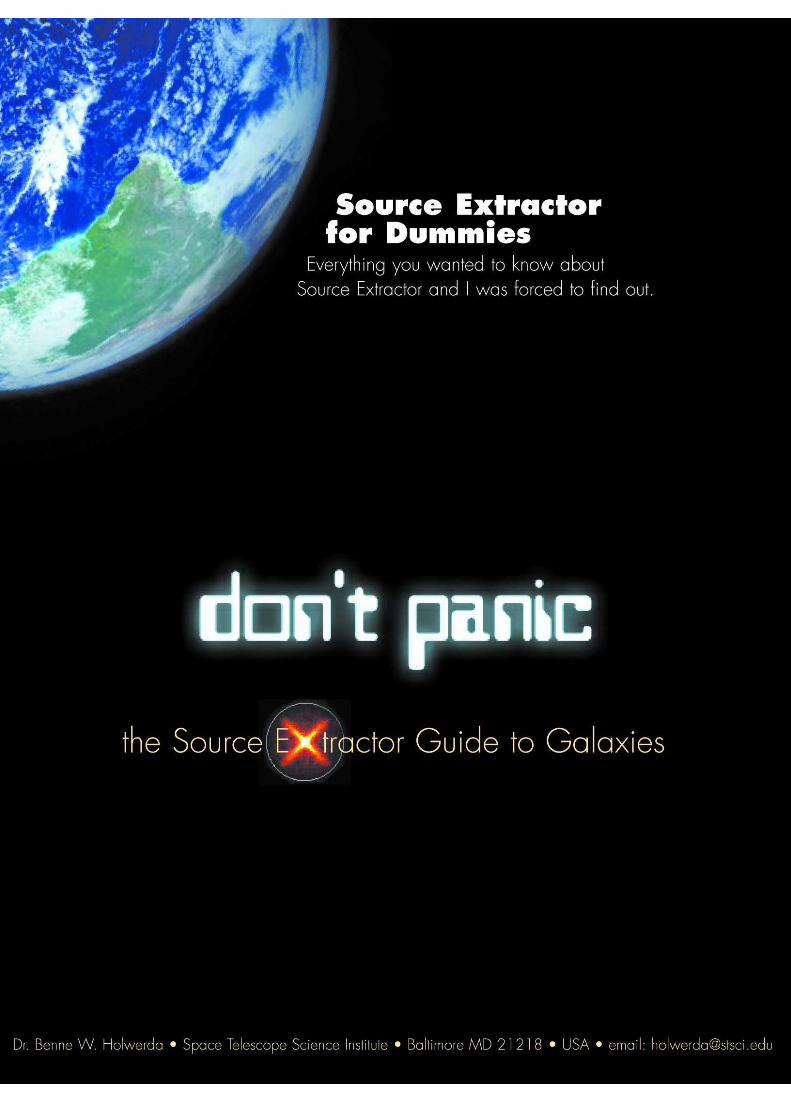

The spiff new cover was made by Robin J. Allen, who also made mythesis-cover. Thank youRobin.
Contents
1 Foreword 7
2 Introduction 9
3 Pros and Cons of SE 11
4 How to install SE 134.1 Installing version 2.2 . . . . . . . . . . . . . . . . . . . . . . . . . . . . . . . 134.2 Installing version 2.3 and up. . . . . . . . . . . . . . . . . . . . . . . . . . . 144.3 Scisoft. . . . . . . . . . . . . . . . . . . . . . . . . . . . . . . . . . . . . . . 14
5 How SE works 15
6 Using SE 196.1 Using SE on one image. . . . . . . . . . . . . . . . . . . . . . . . . . . . . . 196.2 Using SE on separate images for detection and photometry. . . . . . . . . . . . 196.3 Crosscorrellating catalogs. (ASSOC). . . . . . . . . . . . . . . . . . . . . . . 206.4 Multi-extention fits . . . . . . . . . . . . . . . . . . . . . . . . . . . . . . . . 20
7 SE Input: the Configuration File 217.1 Image Information. . . . . . . . . . . . . . . . . . . . . . . . . . . . . . . . . 217.2 Background Estimation. . . . . . . . . . . . . . . . . . . . . . . . . . . . . . 25
7.2.1 Weight Images . . . . . . . . . . . . . . . . . . . . . . . . . . . . . . 277.3 Finding and Separating Objects. . . . . . . . . . . . . . . . . . . . . . . . . . 31
7.3.1 Detection; Thresholds. . . . . . . . . . . . . . . . . . . . . . . . . . . 317.3.2 Filtering . . . . . . . . . . . . . . . . . . . . . . . . . . . . . . . . . . 337.3.3 Deblending: separating into different objects. . . . . . . . . . . . . . . 347.3.4 Cleaning. . . . . . . . . . . . . . . . . . . . . . . . . . . . . . . . . . 36

4 CONTENTS
7.4 Influencing Photometry. . . . . . . . . . . . . . . . . . . . . . . . . . . . . . 367.4.1 ISO . . . . . . . . . . . . . . . . . . . . . . . . . . . . . . . . . . . . 377.4.2 ISOCOR . . . . . . . . . . . . . . . . . . . . . . . . . . . . . . . . . 377.4.3 AUTO . . . . . . . . . . . . . . . . . . . . . . . . . . . . . . . . . . . 387.4.4 BEST . . . . . . . . . . . . . . . . . . . . . . . . . . . . . . . . . . . 397.4.5 Circular Apertures. . . . . . . . . . . . . . . . . . . . . . . . . . . . . 40
7.5 Typical Radii . . . . . . . . . . . . . . . . . . . . . . . . . . . . . . . . . . . 417.5.1 Effective Radii . . . . . . . . . . . . . . . . . . . . . . . . . . . . . . 427.5.2 Kron Radius . . . . . . . . . . . . . . . . . . . . . . . . . . . . . . . 427.5.3 Petrosian Radius. . . . . . . . . . . . . . . . . . . . . . . . . . . . . 427.5.4 Masking Overlapping Objects. . . . . . . . . . . . . . . . . . . . . . . 44
7.6 SE Running . . . . . . . . . . . . . . . . . . . . . . . . . . . . . . . . . . . . 447.6.1 Flags . . . . . . . . . . . . . . . . . . . . . . . . . . . . . . . . . . . 447.6.2 Interpolation. . . . . . . . . . . . . . . . . . . . . . . . . . . . . . . . 457.6.3 Memory Use . . . . . . . . . . . . . . . . . . . . . . . . . . . . . . . 467.6.4 Neural Network. . . . . . . . . . . . . . . . . . . . . . . . . . . . . . 477.6.5 Comments . . . . . . . . . . . . . . . . . . . . . . . . . . . . . . . . 47
7.7 SE output settings. . . . . . . . . . . . . . . . . . . . . . . . . . . . . . . . . 477.7.1 Catalog . . . . . . . . . . . . . . . . . . . . . . . . . . . . . . . . . . 477.7.2 ASSOC parameters. . . . . . . . . . . . . . . . . . . . . . . . . . . . 497.7.3 The Check-images. . . . . . . . . . . . . . . . . . . . . . . . . . . . . 51
8 Output Parameters 558.1 Photometric Parameters. . . . . . . . . . . . . . . . . . . . . . . . . . . . . . 568.2 Profile . . . . . . . . . . . . . . . . . . . . . . . . . . . . . . . . . . . . . . . 588.3 Astrometric Parameters. . . . . . . . . . . . . . . . . . . . . . . . . . . . . . 588.4 Geometric Parameters. . . . . . . . . . . . . . . . . . . . . . . . . . . . . . . 60
8.4.1 Moments . . . . . . . . . . . . . . . . . . . . . . . . . . . . . . . . . 618.4.2 Ellipse parameters. . . . . . . . . . . . . . . . . . . . . . . . . . . . . 618.4.3 Area Parameters. . . . . . . . . . . . . . . . . . . . . . . . . . . . . . 648.4.4 Full-Width Half Max . . . . . . . . . . . . . . . . . . . . . . . . . . . 64
8.5 Radii . . . . . . . . . . . . . . . . . . . . . . . . . . . . . . . . . . . . . . . 658.5.1 Kron radius . . . . . . . . . . . . . . . . . . . . . . . . . . . . . . . . 658.5.2 Petrosian radius. . . . . . . . . . . . . . . . . . . . . . . . . . . . . . 668.5.3 Effective radius. . . . . . . . . . . . . . . . . . . . . . . . . . . . . . 67
8.6 Object classification. . . . . . . . . . . . . . . . . . . . . . . . . . . . . . . . 678.6.1 Input Dependency. . . . . . . . . . . . . . . . . . . . . . . . . . . . . 688.6.2 Reliability . . . . . . . . . . . . . . . . . . . . . . . . . . . . . . . . . 69
8.7 ASSOC output. . . . . . . . . . . . . . . . . . . . . . . . . . . . . . . . . . . 718.8 Flags. . . . . . . . . . . . . . . . . . . . . . . . . . . . . . . . . . . . . . . . 71
8.8.1 Internal Flags. . . . . . . . . . . . . . . . . . . . . . . . . . . . . . . 71

CONTENTS 5
8.8.2 External Flags. . . . . . . . . . . . . . . . . . . . . . . . . . . . . . . 728.9 Fitted Parameters. . . . . . . . . . . . . . . . . . . . . . . . . . . . . . . . . 73
8.9.1 PSF fitting. . . . . . . . . . . . . . . . . . . . . . . . . . . . . . . . . 738.9.2 Galaxy profile fitting . . . . . . . . . . . . . . . . . . . . . . . . . . . 74
8.10 Principle Component. . . . . . . . . . . . . . . . . . . . . . . . . . . . . . . 74
9 Strategies for SE use 779.1 Image types to use?. . . . . . . . . . . . . . . . . . . . . . . . . . . . . . . . 77
9.1.1 Thresholds . . . . . . . . . . . . . . . . . . . . . . . . . . . . . . . . 789.2 How to get faint objects?. . . . . . . . . . . . . . . . . . . . . . . . . . . . . 78
9.2.1 Different Detection Images. . . . . . . . . . . . . . . . . . . . . . . . 789.2.2 Thresholds and Filters. . . . . . . . . . . . . . . . . . . . . . . . . . . 79
9.3 How to get good colours of objects?. . . . . . . . . . . . . . . . . . . . . . . . 799.3.1 separate detection and photometry images?. . . . . . . . . . . . . . . . 809.3.2 which output to use?. . . . . . . . . . . . . . . . . . . . . . . . . . . . 80
9.4 Finding your objects of interest. . . . . . . . . . . . . . . . . . . . . . . . . . 819.5 Strategies to find galaxies in crowded fields. . . . . . . . . . . . . . . . . . . . 81
10 Available Packages 83
11 Follow-up Programs 8511.1 GIM2D . . . . . . . . . . . . . . . . . . . . . . . . . . . . . . . . . . . . . . 8511.2 GALFIT . . . . . . . . . . . . . . . . . . . . . . . . . . . . . . . . . . . . . 85
12 SE use in the Literature 87
13 Known Bugs and Features 91
14 SE parameter additions 93
15 Examples 9515.1 The Data: the Hubble Deep fields. . . . . . . . . . . . . . . . . . . . . . . . . 9515.2 Running the SE default. . . . . . . . . . . . . . . . . . . . . . . . . . . . . . 9615.3 Stars and Galaxies. . . . . . . . . . . . . . . . . . . . . . . . . . . . . . . . . 9615.4 Photometry . . . . . . . . . . . . . . . . . . . . . . . . . . . . . . . . . . . . 9615.5 Typical Radii, source sizes. . . . . . . . . . . . . . . . . . . . . . . . . . . . . 96
16 Acknowledgments 99
A ’Drizzle’ and RMS weight images 101
B SE parameters 103

6 CONTENTS

Chapter 1
Foreword
Sextractor for dummies is not a book in the famous series, I just liked the title. Sextractor is not atoy for grownups, it is a extremely usefull and versatile astronomical (and perhaps other disiplines)softwaretool.In the course of my PhD I learned a great deal about it by trial and error and from Ed Smith andmany others. To have somewhere to explain every knob and dialis the motivation behind this man-ual.1 I hope to make it as accurate and complete and possibly even complete as possible. I hope ithelps with whatever project you are working on.
There has been quite some time between updates of this user manual. I apologize but certainexternal factors insisted I write a PhD thesis first. In the meantime, both the official documentationand the program have been updated. I hope I’ve now caught up sufficiently that this is again auseful manual for the beginning and advanced source extractor user.2
1Yes my motto is “Never read a manual as long there are still buttons and levers left...” but in sextractor’s case youmight want to make an exception. Besides I’m perfectly happyif you just skim it.
2And if you find a problem, inconsistency or spelling erro...please drop me a line [email protected]

8 CHAPTER 1: FOREWORD
Chapter 2
Introduction
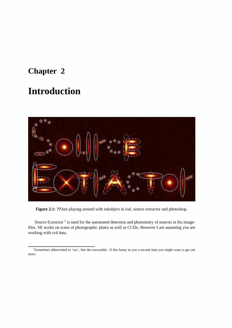
Figure 2.1: ??Just playing around with mkobject in iraf, source extractorand photoshop.
Source Extractor1 is used for the automated detection and photometry of sources in fits image-files. SE works on scans of photographic plates as well as CCDs. However I am assuming you areworking with ccd data.
1Sometimes abbreviated to ’sex’, like the executable. If this funny to you a second time you might want to get outmore.

10 CHAPTER 2: INTRODUCTION
If you goal is to get catalogs of all the detected objects withreasonably goodphotometry from aFITSfile of processed astronomical imaging data, then SEis the instrument you need.2
If you want REALLY good photometry on only a few objects and you know where they are,do not use SE. I’ll discuss how SE works and subsequently how to start it and which parameters dowhat and what the different parameters in the catalogs mean.Some, but by no means all, strategiesfor its use are discussed and to illustrate some examples from my own experiences will be given.
This started as a bunch of notes of mine and Ed Smith and is evolving slowly beyond that. Ihope to provide for slightly more insight into SE than the official manual for two reasons: first, allthe parameters (both input and output) will be discussed in one document, making it slightly morecomplete than either of the manuals and secondly it has DON’TPANIC written in large friendlyletters on the cover.

Chapter 3
Pros and Cons of SE
As I tried to point out in the introduction and will emphasizeoccasionally SE is not suited forevery astronomy project that needs photometry of objects ina field. As everything, it has strongand weak points.
The pros of SE are listed in the manual but the most important ones are:
1. Speed. SE is made to go through data quickly. And if you’re trying to beaver through severalsquare degrees of data, speed is GOOD.
2. The capacity to handle large fits files. SE is coded up so thatit’ll take it a piece at a time.Again good for the sky-eaters among us.
3. Works on CCD and scanned photographic plate data. Nice if you happen to have this kindof data.
4. Does decent photometry.
5. Robust, it’ll run with idiotic input.
6. Controllable, most steps can be influenced by user.
7. The possibility to accept user specified flag images or weight images.
8. Output parameters and the order in which these are listed,are specified by the user.
8. Output image-files depicting apertures, detections and more.
9. The possibility to detect sources in one image and do the photometry in another.
10. There is follow-up software to decomposition of galaxy profiles. Source identification anda first selection can be done with source extractor and eitherGIM2D or GALFIT can thenfollow-up.

12 CHAPTER 3: PROS AND CONS OFSE
However SE has some drawbacks. It was made for speedy use and in some case accuracy hasbeen sacrificed for speed on purpose. So here is the other sideof the coin:
1. Only as good as its settings. SE is dependent on some of it’ssetting and these are crucial forthe detection and photometry. It will run on just about any set of input parameters but giveback output that may be total bogus.
2. Manuals are outdated and incomplete. This handbook is written as a remedy for that but bya user and not the person who wrote the code.1
3. Limited accuracy. You’ll see this with the geometrical output parameters. These are com-puted (from moments), NOT fitted (which would be more accurate).
4. Classification of objects is ofvery limited use.
5. Breaks down in crowded fields eventually.
6. Corrections of photometry for the ’wings’ of object profiles is very rudimentary.
But as long as you, the user are aware of these little drawbacks and use the SE input as a fiststart to fit with GIM2D or something then all will be well.
1So I’m NOT claiming completeness or correctness.
Chapter 4
How to install SE
4.1 Installing version 2.2
First you get the most recent version of SE fromhttp://terapix.iap.fr/soft/sextractor/index.html.Then you unzip and tar the file (UNIX):
gzip -dc sex_2.2.2.tar.gz | tar xv
That should leave you with a directory in the directory whereyou did this calledsextrac-tor2.2.2/ with instructions on how to install in ’INSTALL’. Basicallyyou go to the ’sextrac-tor2.2.2/source’ directory and type:
make SEXMACHINE= ’machine type’
where the ’machine type’ can be any of the following possibilities:
aix (for IBMs RS6000 running AIX)alpha (for DEC-ALPHAs with Digital UNIX)hpux (for HP/UX systems)linuxpc (for PCs running LINUX, using gcc)linuxp2 (for Pentium2/3/4 PCs running LINUX)linuxk7 (for Athlon PCs running LINUX)sgi (for SGI platforms)solaris (for SUN-Solaris machines)sunos (for SUN-OS platforms)ultrix (for DEC stations running ULTRIX)
The SE manual is available in postscript format to you in the ’sextractor2.2.2/doc’ directory.Congrats, you have Source Extractor available as an executable ’sex’ in the ’sextractor2.2.2/source’directory. The ’make’ file tries to make a shortcut to this executable in your ’home’ directory. If thisfails, try making an alias for the command or simply type the whole path/wherever/sextractor2.2.2/source/sex.

14 CHAPTER 4: HOW TO INSTALL SE
4.2 Installing version 2.3 and up
The simplest way to compile this package is:
1. ‘cd’ to the directory containing the package’s source code and type ‘./configure’ to configurethe package for your system.
2. Type ‘make’ to compile the package.
3. Type ‘make install’ to install the programs and any data files and documentation.
But if you use linux, the rpm files are also available.
4.3 Scisoft
At the European Southern Observatory, a package of all interesting scientific software is being keptup to date and easy to install. Source extractor is part of this package and since the installation isalmost plug-and-do-science (for the mac at least...). I highly recommend it, especially the Mac.1
get it here:
http://www.eso.org/science/scisoft/ (LINUX)http://www.stecf.org/macosxscisoft/ (Mac OSX)
1Ok....I’ve plugged this enough.
Chapter 5
How SE works
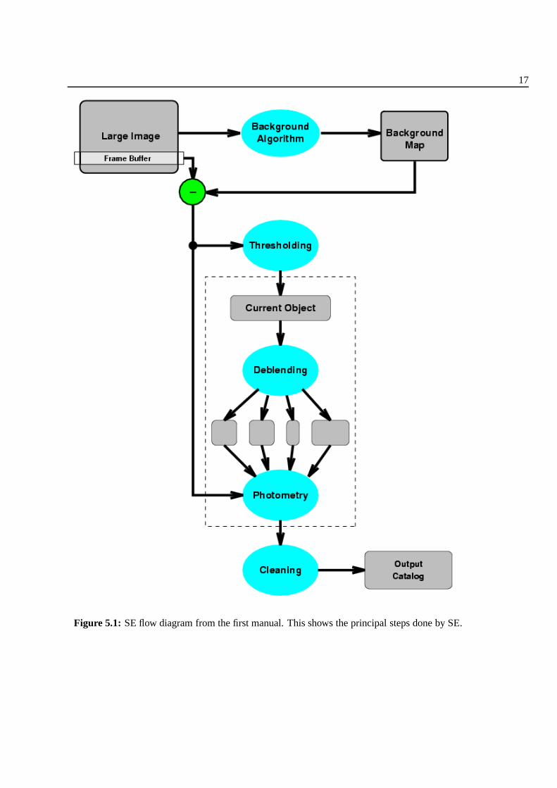
The source extractor package works in a series of steps. It determines the background and whetherpixels belong to background or objects. Then it splits up thearea that is not background intoseparate objects and determines the properties of each object, writing them to a catalog.
The background determination is treated in the official manual and in section 7.2 All the pixelsabove a certain threshold are taken to belong to an object. Ifthere is a saddle point in the inten-sity distribution (there are two peaks in the light distribution distinct enough), the object is split indifferent entries in the catalogs. Photometry is done on these by dividing up the intensity of theshared pixels. There is an option to ”clean ” the catalog in order to eliminate artifacts caused bybright objects. Afterward, there is a list of objects with a series of parameters measured (ellipticity,size etc.). These are classified into stars and galaxies (everything non-star) by a neural network.
The first steps are controlled by a number of parameters. How to estimate the threshold? Howmuch contrast should there be to split an object? However, the classification by the neural net-work only depends indirectly on the parameters controllingthe first steps. As the network has beentrained on ground based data, there might be some doubts on the reliability of this classification asone switches to other passbands or instruments. So check up on this classification in the case offaint or blended objects.
Some of the steps in SE have maps associated with them and these can be written to fits files,the ’check’ images.
Aside from the input image, SE can handle weightimages and flag-images to mark the relativeimportance of pixels or to flag bad ones.
The fitting of the Point-Spread-Function is not yet operational but it was already indicated inthe second flow diagram in manual version 2.1.3.
Steps of SE:
1. Measure the background and its RMS noise (background and RMS maps). (6.2)
2. Subtract background.

16 CHAPTER 5: HOW SE WORKS
3. Filter (convolve with specified profile). (6.3.2)
4. Find objects (thresholding). (6.3.1)
5. Deblend detections (break up detection into different objects. (6.3.3)
6. Measure shapes and positions.
7. Clean (reconsider detections, accounting for contributions from neighbors) (6.3.4)
8. Perform photometry.
9. Classify/index level of fuzziness –¿ more star-like or galactic?
10. Output Catalog and ’Check’ Images
17
Figure 5.1: SE flow diagram from the first manual. This shows the principalsteps done by SE.

18 CHAPTER 5: HOW SE WORKS
Figure 5.2: SE flow diagram from the second manual. This shows clearly themany extra optionsover a simple run of SE; the possibilities of weight maps, flags, crosscorellation catalogs and manymore.
Chapter 6
Using SE
Source Extractor can be used in basically three ways: on a single file for both detection and pho-tometry, on two files, one for detection, the other for photometry and on two files with cross-identification in the catalogs.
6.1 Using SE on one image
SE needs a series of parameters in order to run and these can begiven at the command line or in aconfiguration file. So to run SE on a single file with all the necessary parameters in the configura-tion file one types:
seximage-c configurationfile.txt
If there is no configuration file given, SE will try to read ’default.sex’ from the local directory.However, the parameter values can be fed to SE on the command line as well:
seximage-c configurationfile.txt -PARAMETER1value1-PARAMETER2value2
The names of the parameters and their meanings and preferredvalues are discussed below.
NOTE: if you use both a configuration file and command line parameter input,the command line input takes precedence over the configuration file value.
6.2 Using SE on separate images for detection and photometry
This may sound weird but the option in SE to find all the objectsin one image and then apply theapertures and positions found on another image can be quite useful. To useimage1for the detection
20 CHAPTER 6: USING SE
of sources andimage2for the photometry:
seximage1,image2-c configurationfile.txt
Suppose you want different colors or color information fromthe series of images you have indifferent filters. It is in that case very convenient to use the same apertures. So provided the imagesare well aligned,1 the photometry done is essentially the same objects using the same apertures.2
The nice part is that the numbering in the catalogs in this dual mode and the numbering in thesingle mode on the first image are the same. It should spare youa lot of rooting around in thecatalogs if you want to compare fluxes in different bands for instance. This particular feature isfurther discussed in the strategy section.
6.3 Crosscorrellating catalogs. (ASSOC)
There is a third possibility to get information on objects that occur in separate images, for instancein overlapping fields in a survey or simulated objects in the SE detections. Basically you run SEon one field and take the X and Y positions (in pixels) from the catalogs and feed them to SE in asecond run with a search radius and a priority (the brightestassociation or the nearest? etc.) Andthe matches are printed in a new catalog. See the ASSOC parameters in the catalog configurationsection.
6.4 Multi-extention fits
There is a new feature in Source extractor. It now supports multiple extension fits files. FITSis now the ’standard’ filetype3 for astronomical observations and several images can be part of asingle fits-file. Many new data-products now include weight and quality maps of the astronomicalimage4.
1The bright sources are on the same pixels, check by loading both in saotng or another display package and then’blink’ between them. If you’re drizzling or stacking several exposures, use the same reference image.
2If you want awfully good photometry then it might be good te realize that a point spread function correction isdependent on the filter used. But keep in mind that SE does not do THAT good photometry to start with.
3As with standards, everyone seems to have their own.4The Advanced Camera for Surveys on board HST for instance.
Chapter 7
SE Input: the Configuration File
”On two occasions, I have been asked [by members of Parliament], ’Pray, Mr. Babbage, if youput into the machine wrong figures, will the right answers come out?’ I am not able to rightly
apprehend the kind of confusion of ideas that could provoke such a question.”– Charles Babbage1
As stated in the previous section, SE tries to read the configuration file default.sexor a filecan be given on the command line.2 Thedefault.sexcan be found in the/sextractor-2.4.4/config/directory. It gives a good set of defaults for SE to use.
The configuration file is good way of remembering which parameters you used in running SEand you do not have to reset all the parameters when running SEover a series of files. The config-uration file is an ASCII file (plain text) with the name of the parameters and the value on separatelines. A comment line begins with ’#’ and ends with the end-of-line.
The parameters are listed alphabetically in the manual. I discuss them here in topical order.Input parameters for SE can be roughly divided into the following categories: image information,background estimation, detection, photometry, catalogs and SE running parameters.
7.1 Image Information
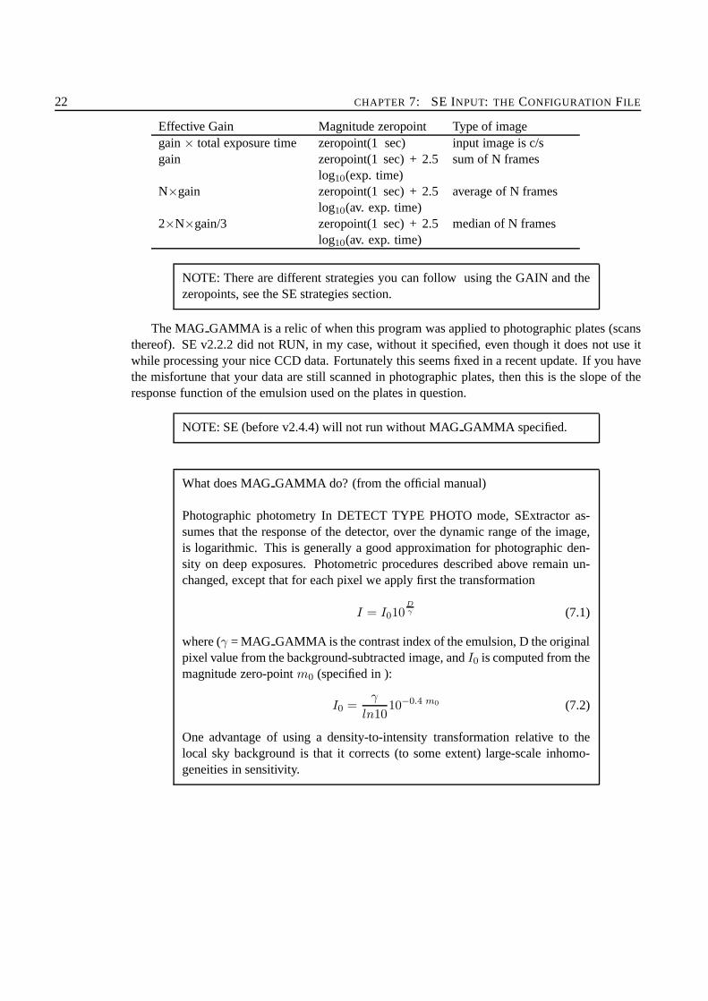
SE gets the positional information from the FITS header but most of the following parameters mustbe specified. GAIN is the ratio of the number of electrons to the number of ADU. The GAIN isdependent on the type of CCD you’re using and the instrument in front of it (for instance the WF2chip on the HST has a gain of 7).
How the number you use here, the effective gain, relates to the instrument gain is as follows:
1Morale: input is inportant...2If the idea of having.sexfiles littering your hard disk is a little too randy for you, SEwill read in any ASCII text
files it is given as a configuration file.
22 CHAPTER 7: SE INPUT: THE CONFIGURATION FILE
Effective Gain Magnitude zeropoint Type of imagegain× total exposure time zeropoint(1 sec) input image is c/sgain zeropoint(1 sec) + 2.5
log10(exp. time)sum of N frames
N×gain zeropoint(1 sec) + 2.5log10(av. exp. time)
average of N frames
2×N×gain/3 zeropoint(1 sec) + 2.5log10(av. exp. time)
median of N frames
NOTE: There are different strategies you can follow using the GAIN and thezeropoints, see the SE strategies section.
The MAG GAMMA is a relic of when this program was applied to photographic plates (scansthereof). SE v2.2.2 did not RUN, in my case, without it specified, even though it does not use itwhile processing your nice CCD data. Fortunately this seemsfixed in a recent update. If you havethe misfortune that your data are still scanned in photographic plates, then this is the slope of theresponse function of the emulsion used on the plates in question.
NOTE: SE (before v2.4.4) will not run without MAGGAMMA specified.
What does MAGGAMMA do? (from the official manual)
Photographic photometry In DETECT TYPE PHOTO mode, SExtractor as-sumes that the response of the detector, over the dynamic range of the image,is logarithmic. This is generally a good approximation for photographic den-sity on deep exposures. Photometric procedures described above remain un-changed, except that for each pixel we apply first the transformation
I = I010Dγ (7.1)
where (γ = MAG GAMMA is the contrast index of the emulsion, D the originalpixel value from the background-subtracted image, andI0 is computed from themagnitude zero-pointm0 (specified in ):
I0 =γ
ln1010−0.4 m0 (7.2)
One advantage of using a density-to-intensity transformation relative to thelocal sky background is that it corrects (to some extent) large-scale inhomo-geneities in sensitivity.

IMAGE INFORMATION 23
The DETECTTYPE specifies what type of data SE is handling, scanned photoplates orCCD data. Even with DETECTTYPE set to CCD, older versions of SE will still need thatMAG GAMMA.
MAG ZEROPOINT is the zeropoint for the photometric measurements. This is again differentif you use counts-per-second images as opposed to total counts images. The counts-per-secondimages have the zeropoint specified by the instrument handbook (depends on filter, instrumentand type of ccd used). But in the case of a total counts image isthe handbook value plus the2.5 log10(exposuretime).
PIXEL SCALE is again something you hopefully know before you started to run SE. Funnyenough this is not read from the Fits header. So specify this!SE needs itonly for the CLASSSTARparameter (but still needs it).
NOTE: New feature in SE (v2.4.4.). When this parameter is setto 0, SE usesthe World coordinate fits information to compute the pixelscale.
SATUR LEVEL is the limit for SE to start extrapolating to get the photometry. However assoon as you hit something as saturated as that you might want to see if there is another way todetermine the flux from that object.
The SEEINGFWHM (Full Width at Half Maximum) is important for that separation betweenstars and galaxies. Like the PIXELSCALE it is only used for the CLASSSTAR parameter.3
3Seeing is the blurring of the image as a result of atmosphericdisturbances (cirrus clouds, turbulence etc.). Anestimate of the seeing should be documented in either the header or the observation logs. If not, make something up,possibly inspired by that looks like a bright star.
24 CHAPTER 7: SE INPUT: THE CONFIGURATION FILE
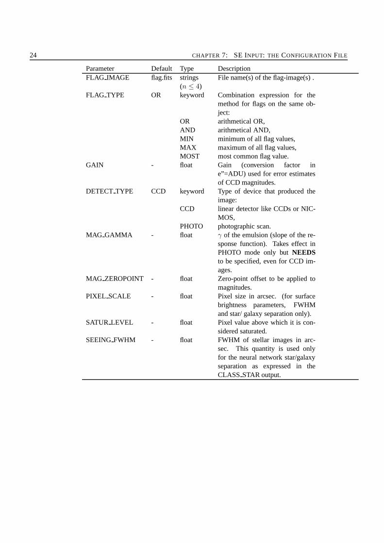
Parameter Default Type DescriptionFLAG IMAGE flag.fits strings
(n ≤ 4)File name(s) of the flag-image(s) .
FLAG TYPE OR keyword Combination expression for themethod for flags on the same ob-ject:
OR arithmetical OR,AND arithmetical AND,MIN minimum of all flag values,MAX maximum of all flag values,MOST most common flag value.
GAIN - float Gain (conversion factor ine”=ADU) used for error estimatesof CCD magnitudes.
DETECT TYPE CCD keyword Type of device that produced theimage:
CCD linear detector like CCDs or NIC-MOS,
PHOTO photographic scan.MAG GAMMA - float γ of the emulsion (slope of the re-
sponse function). Takes effect inPHOTO mode only butNEEDSto be specified, even for CCD im-ages.
MAG ZEROPOINT - float Zero-point offset to be applied tomagnitudes.
PIXEL SCALE - float Pixel size in arcsec. (for surfacebrightness parameters, FWHMand star/ galaxy separation only).
SATUR LEVEL - float Pixel value above which it is con-sidered saturated.
SEEINGFWHM - float FWHM of stellar images in arc-sec. This quantity is used onlyfor the neural network star/galaxyseparation as expressed in theCLASS STAR output.
BACKGROUND ESTIMATION 25
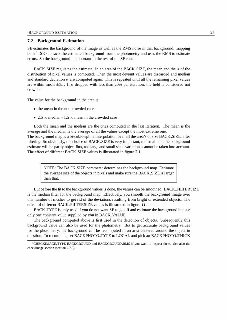
7.2 Background Estimation
SE estimates the background of the image as well as the RMS noise in that background, mappingboth4. SE subtracts the estimated background from the photometryand uses the RMS to estimateerrors. So the background is important in the rest of the SE run.
BACK SIZE regulates the estimate. In an area of the BACKSIZE, the mean and theσ of thedistribution of pixel values is computed. Then the most deviant values are discarded and medianand standard deviationσ are computed again. This is repeated until all the remainingpixel valuesare within mean±3σ. If σ dropped with less than 20% per iteration, the field is considered notcrowded.
The value for the background in the area is:
• the mean in the non-crowded case
• 2.5× median - 1.5× mean in the crowded case
Both the mean and the median are the ones computed in the last iteration. The mean is theaverage and the median is the average of all the values exceptthe most extreme one.The background map is a bi-cubic-spline interpolation overall the area’s of size BACKSIZE, afterfiltering. So obviously, the choice of BACKSIZE is very important, too small and the backgroundestimate will be partly object flux, too large and small scalevariations cannot be taken into account.The effect of different BACKSIZE values is illustrated in figure 7.1.
NOTE: The BACKSIZE parameter determines the background map. Estimatethe average size of the objects in pixels and make sure the BACK SIZE is largerthan that.
But before the fit to the background values is done, the valuescan be smoothed: BACKFILTERSIZEis the median filter for the background map. Effectively, yousmooth the background image overthis number of meshes to get rid of the deviations resulting from bright or extended objects. Theeffect of different BACKFILTERSIZE values is illustrated in figure??.
BACK TYPE is only used if you do not want SE to go off and estimate thebackground but useonly one constant value supplied by you in BACKVALUE.
The background computed above is first used in the detection of objects. Subsequently thisbackground value can also be used for the photometry. But to get accurate background valuesfor the photometry, the background can be recomputed in an area centered around the object inquestion. To recompute, set BACKPHOTOTYPE to LOCAL and pick an BACKPHOTOTHICK
4CHECKIMAGE TYPE BACKGROUND and BACKGROUNDRMS if you want to inspect them. See also thecheckimage section (section 7.7.3).
26 CHAPTER 7: SE INPUT: THE CONFIGURATION FILE
to match your tastes (generally speaking, somewhat larger than the objects in questions would be agood idea).
NOTE: the RMS as determined from the BACKGROUNDRMS map will beused in more than just the photometry, the thresholds for detection and analysiscan be dependent on it.
NOTE: if you want to subtract the background and not have SE dothis for you,set BACK TYPE to MANUAL and BACK VALUE to 0.0,0.0
BACK_SIZE 64 BACK_SIZE 128
BACK_SIZE 512
BACK_SIZE 16 BACK_SIZE 32
BACK_SIZE 256
HDF
Figure 7.1: The HDF-N with the background estimates using different BACK SIZE values.Clearly a BACKSIZE smaller than the biggest objects will result in a too much variation in thebackground estimate. A overlarge BACKSIZE will not account for variations in background.Grayscales for the background field are the same.

BACKGROUND ESTIMATION 27
Parameter Default Type DescriptionBACK SIZE - integers
(n ≤ 2)Size, or Width, Height (inpixels) of a backgroundmesh.
BACK FILTERSIZE - integers(n ≤ 2)
Size, or Width, Height (inbackground meshes) ofthe background-filteringmask.
BACK TYPE AUTO keywords(n ≤ 2)
What background is sub-tracted from the images:
AUTO The internal interpolatedbackground-map. In themanual it says “INTER-NAL” here but the key-word is AUTO.
MANUAL A user-supplied constantvalue provided in BACKVALUE.
BACK VALUE 0.0,0.0 floats(n ≤ 2)
in BACK TYPE MAN-UAL mode, the constantvalue to be subtractedfrom the images.
BACKPHOTO THICK 24 integer Thickness (in pixels) ofthe background LOCALannulus.
BACKPHOTO TYPE GLOBAL keyword Background used to com-pute magnitudes:
GLOBAL taken directly from thebackground map,
LOCAL recomputed in a rectangu-lar annulus around the ob-ject.
7.2.1 Weight Images
The individual pixels in the detection image can be given relative importance by using a weight foreach of them. Different options are available: the background as determined by SE or an externalweight image. If an external weight image is given, it has to be specified what kind it is; a variancemap or a rms map or a weight map, from which a variance map should be derived.
The weight for each pixel is derived as follows:

28 CHAPTER 7: SE INPUT: THE CONFIGURATION FILE
HDF BACK_FILTERSIZE = 3
BACK_FILTERSIZE = 5
BACK_FILTERSIZE = 1
BACK_FILTERSIZE = 7 BACK_FILTERSIZE = 9
BACK_FILTERSIZE = 11
Figure 7.2: The HDF-N with the background estimates using different BACK FILTERSIZEvalues. The mesh of background estimates (BACKSIZE = 64) is smoothed over theBACK FILTERSIZE before interpolating into the BACKGROUND map.
weight =1
variance=
1
rms2
WEIGHT TYPE MAP WEIGHT is directly taken as the weight, WEIGHTTYPE MAP VARis inverted and WEIGHTTYPE MAP RMS is squared and inverted.
Reasons for using a weight image are various but to give you anidea: SE can ignore pieces ofthe image this way, use a flat-field in it’s photometry or edited results from a previous run.5
Users of the stsdasdrizzlepackage should check out the appendix on drizzle’s weight image.These are the parameters controlling it:
I can’t really fathom why WEIGTHGAIN isn’t simply an option in WEIGHTTYPE but itisn’t. So there.
WEIGHT IMAGE is the input parameter where the⁀fits file is given which is to be used asweight map of the type defined by the WEIGHTTYPE parameter.
With WEIGHT TYPE set on BACKGROUND, the ’checkimage’ (output image withCHECKIM-AGE TYPE set on BACKGROUND) of a previous run can be used. MAPRMS can be for instance
5Please note that I do not specify by what kind of black magic you obtained these weight images. They may be theresult from a previous SE run but a ccd dark-frame might be used. Or perhaps your data-reduction scheme will producea good estimate of the rms. To be used with caution!

BACKGROUND ESTIMATION 29
derived from known noise characteristics of the instrumentor given by other programs used in data-reduction (for instance the ’drizzle’ package for HST data).
Parameter Default Type DescriptionWEIGHT GAIN Y boolean If true, weight maps are consid-
ered as gain maps.WEIGHT IMAGE weight.fits strings
(n ≤ 2)File name of the detection andmeasurement weightimage , re-spectively.
WEIGHT TYPE NONE keywords(n ≤ 2)
Weighting scheme (for singleimage, or detection and mea-surement images):
NONE no weighting,BACKGROUND
variance-map derived from theimage itself,
MAP RMS variance-map derived from anexternal RMS-map,
MAP VAR external variance-map,MAP WEIGHT
variance-map derived from anexternal weight-map,
NOTE: WEIGHT TYPE set to BACKGROUND does NOT mean that theweight image will be used for the background determination.
30 CHAPTER 7: SE INPUT: THE CONFIGURATION FILE
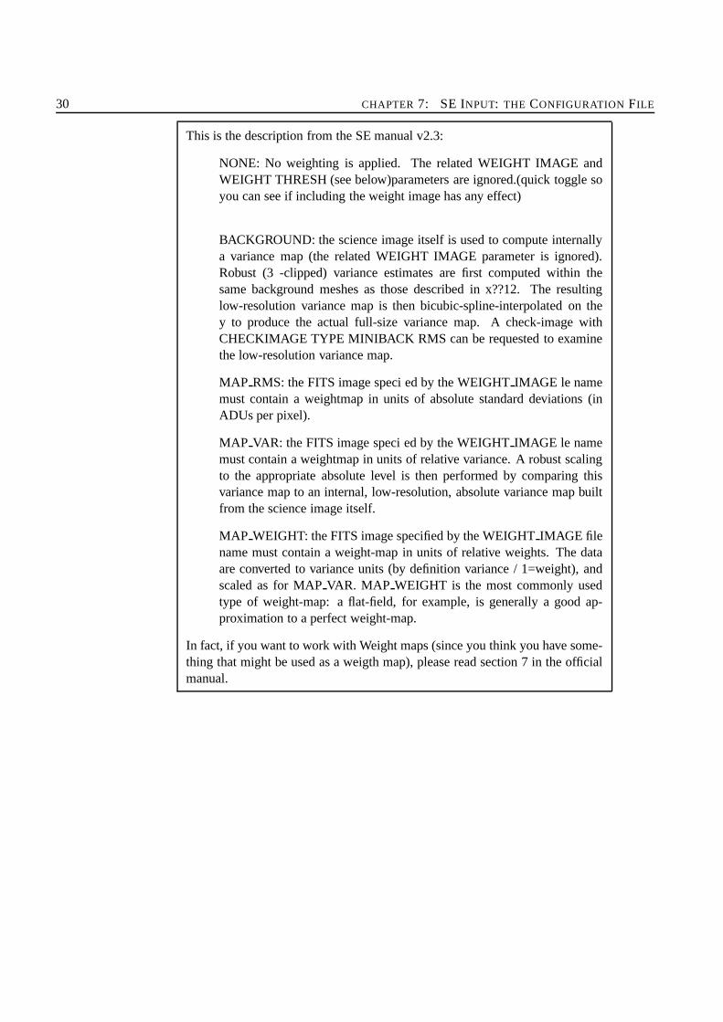
This is the description from the SE manual v2.3:
NONE: No weighting is applied. The related WEIGHT IMAGE andWEIGHT THRESH (see below)parameters are ignored.(quick toggle soyou can see if including the weight image has any effect)
BACKGROUND: the science image itself is used to compute internallya variance map (the related WEIGHT IMAGE parameter is ignored).Robust (3 -clipped) variance estimates are first computed within thesame background meshes as those described in x??12. The resultinglow-resolution variance map is then bicubic-spline-interpolated on they to produce the actual full-size variance map. A check-image withCHECKIMAGE TYPE MINIBACK RMS can be requested to examinethe low-resolution variance map.
MAP RMS: the FITS image speci ed by the WEIGHTIMAGE le namemust contain a weightmap in units of absolute standard deviations (inADUs per pixel).
MAP VAR: the FITS image speci ed by the WEIGHTIMAGE le namemust contain a weightmap in units of relative variance. A robust scalingto the appropriate absolute level is then performed by comparing thisvariance map to an internal, low-resolution, absolute variance map builtfrom the science image itself.
MAP WEIGHT: the FITS image specified by the WEIGHTIMAGE filename must contain a weight-map in units of relative weights.The dataare converted to variance units (by definition variance / 1=weight), andscaled as for MAPVAR. MAP WEIGHT is the most commonly usedtype of weight-map: a flat-field, for example, is generally a good ap-proximation to a perfect weight-map.
In fact, if you want to work with Weight maps (since you think you have some-thing that might be used as a weigth map), please read section7 in the officialmanual.

FINDING AND SEPARATING OBJECTS 31
7.3 Finding and Separating Objects
SE considers every pixel above a certain threshold (to be specified by YOU6 , directly or indirectly)to be part of an object. The ’deblending’ is the part where it figures out which pixels or parts ofpixels belong to which objects.
7.3.1 Detection; Thresholds
The threshold parameters indicate the level from which SE should start treating pixels as if theywere part of objects, determining parameters from them. There are three requirements for a candi-date objects:
1. All the pixels are above the DETECTTHRESH.
2. All these pixels are adjacent to each other (either corners or sides in common).
3. There are more than the minimum a number of pixels (specified in DETECTMINAREA).
ANALYSIS THRESH is just the threshold for CLASS STAR and FWHM, all the other param-eters are determined from the DETECTTHRESH.
NOTE: All the OTHER analysis (photometry and the like) is done with theDETECT THRESH!
They can both be specified in three ways:
• In Surface Brightness: SBlimit,SBzeropoint e.g. DETECTTHRESH 23.5, 24
• In ADU’s (set THRESHTYPE ABSOLUTE) e.g. DETECTTHRESH 1.2
• Relative to background RMS (set THRESHTYPE RELATIVE) e.g. DETECTTHRESH1.2 (this is the initial setup in the default.sex file.)
The threshold in surface brightness mu (mag/arcsec2 ) needs a calibration Zero-point (mag/arcsec2
corresponding to 0 counts). Note that this can/will be different from the MAGZEROPOINT value.7
NOTE: This whole SB threshold stuff seems quite the thing until you realizeSE just does this:
thresh = 10−SBlimit−SBzeropoint
2.5
6yes YOU! You did it to yourself, you and only you and that’s what really hurts. (Radiohead)7For the HST instruments, the zeropoints can be obtained using CALCPHOT in the stsdas package in IRAF. Re-
member that these are dependent on instrument and filter.

32 CHAPTER 7: SE INPUT: THE CONFIGURATION FILE
With THRESHTYPE set to ABSOLUTE, the threshold is set to the same number of ADUsacross the image. If THRESHTYPE set to RELATIVE (the default), the the threshold is thatnumber of background RMS standard deviations above the background value. This is nice andflexible but sensitive to the background estimation!
The DETECTMINAREA is the minimum number of pixels above the threshold required to beconsidered an object.
7
������������������������������������������������������������
������������������������������������������������������������
1 2 3
8 4
56
Figure 7.3: An object is defined as a series of bordering pixels above the threshold. Borderingpixels to the gray one are 1 through 8. Another pixels needs tobe above the threshold and share acorner or a side with another pixel in order to considered part of the same object (unless they aredeblended into different objects).

FINDING AND SEPARATING OBJECTS 33
Parameter Default Type DescriptionTHRESHTYPE RELATIVE keywords
(n ≤ 2)Meaning of the DE-TECT THRESH andANALYSIS THRESHparameters :
RELATIVE scaling factor to thebackground RMS,
ABSOLUTE absolute level (in ADUsor in surface brightness).
ANALYSIS THRESH - floats (n ≤2)
Threshold (in surfacebrightness) at whichCLASS STAR andFWHM operate. 1argument: relative toBackground RMS.2 arguments: mu(mag/arcsec”2 ),Zero-point (mag).
DETECT THRESH - floats (n ≤2)
Detection threshold. 1argument: (ADUs orrelative to BackgroundRMS, see THRESHTYPE). 2 arguments:R (mag.arcsec” 2 ),Zero-point (mag).
DETECT MINAREA - integer Minimum number ofpixels above thresholdtriggering detection.
7.3.2 Filtering
Before the detection of pixels above the threshold, there isthe option of applying a filter. This filteressentially smooths the image.8
There are some advantages to applying a filter before detection. It may help detect faint, ex-tended objects
However it may not be so helpful if your data are very crowded.There are four types of filter tobe found in the./sextractor2.2.2/config/directory; Gaussian, Mexican hat, tophat and blokfunctionof various sizes, all normalized.
This is what the helpful README in this directory tells us:
8The photometry is still being done on the original image, don’t worry.

34 CHAPTER 7: SE INPUT: THE CONFIGURATION FILE
Name Descriptiondefault.conv a small pyramidal function (fast)gauss*.conv a set of Gaussian functions, for seeing FWHMs between 1.5
and 5 pixels (best for faint object detection).tophat*.conv a set of ”top-hat” functions. Use them to detect extended, low-
surface brightness objects, with a very low THRESHOLD.mexhat*.conv ”wavelets”, producing a passband-filtering of the image, tuned
to seeing FWHMs between 1.5 and 5 pixels. Useful in verycrowded star fields, or in the vicinity of a nebula. WARNING:may need a high THRESHOLD!!
block 3x3.conv a small ”block” function (for rebinned images likethose of theDeNIS survey).
The naming convention seems to be: nameseeingFWHMsize.conv. Both the seeing FWHMand the size are in pixels. So depending on what you are after,choose a filter and approximatelyyour seeing.
NOTE: filter choice and threshold choice are interdependent!
Parameter Default Type DescriptionFILTER - boolean If true, filtering is applied to the
data before extraction.FILTER NAME - string Name and path of the file con-
taining the filter definition.FILTER THRESH - floats (n ≤
2)Lower and higher thresholds(in back-ground standard devia-tions) for a pix-el to be consid-ered in filtering (used for retina-filtering only).
7.3.3 Deblending: separating into different objects
Deblending is the part of SE where a decision is made whether or not a group of adjacent pixelsabove DETECTTHRESH is a single object or not. Suppose there is a little island of adjacentpixels above the threshold. It is an object or maybe several really close next to each other. So howdoes SE cut this up into different objects? First it defines a number of levels between the thresholdand the maximum count in the object. This is set by the DEBLENDNTHRESH parameter. Thelevels are spaced exponentially.
SE then constructs a ’tree’ of the objects, branching every time there are pixels above a thresh-old separated by pixels below it (see figure). A branch is considered a different object provided:
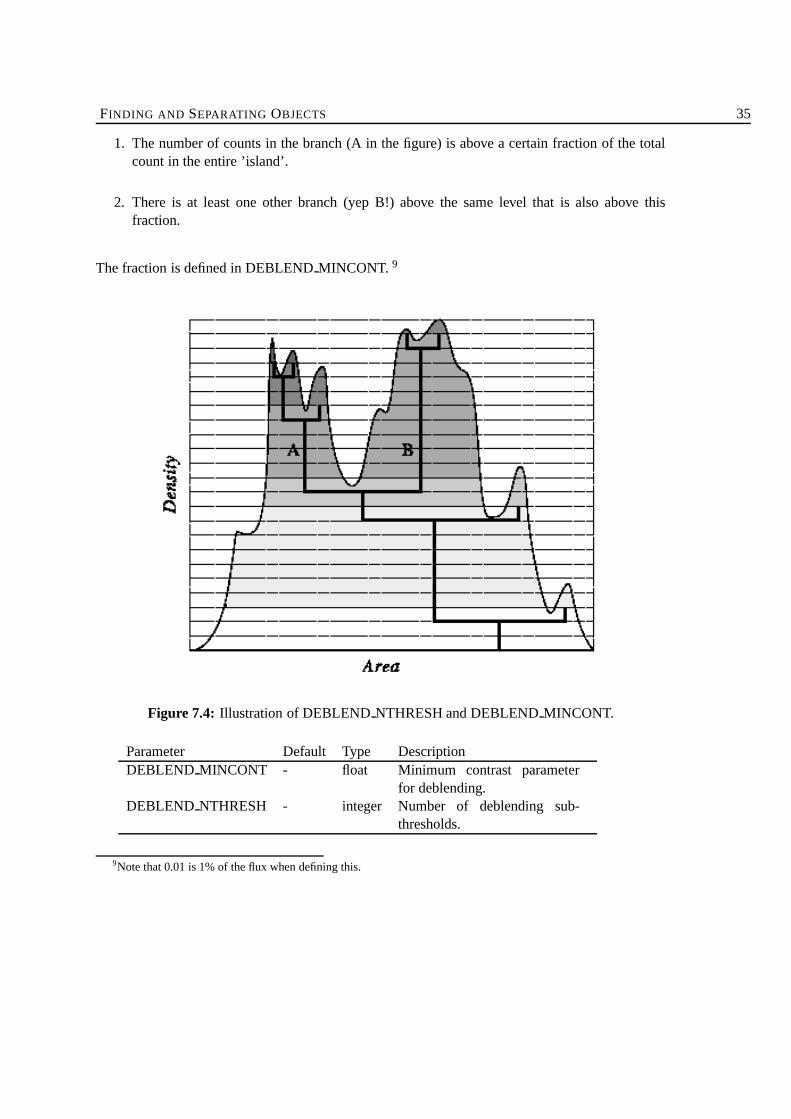
FINDING AND SEPARATING OBJECTS 35
1. The number of counts in the branch (A in the figure) is above acertain fraction of the totalcount in the entire ’island’.
2. There is at least one other branch (yep B!) above the same level that is also above thisfraction.
The fraction is defined in DEBLENDMINCONT. 9
Figure 7.4: Illustration of DEBLENDNTHRESH and DEBLENDMINCONT.
Parameter Default Type DescriptionDEBLEND MINCONT - float Minimum contrast parameter
for deblending.DEBLEND NTHRESH - integer Number of deblending sub-
thresholds.
9Note that 0.01 is 1% of the flux when defining this.
36 CHAPTER 7: SE INPUT: THE CONFIGURATION FILE
7.3.4 Cleaning
There is the option to ’clean’ the list of objects of artifacts due to bright objects (set CLEAN toYES). All the detections are checked to see if they would havebeen detected (i.e. exceeded thethreshold etc.) if their neighbors were not there. To do this, the contributions of the neighboringobjects has to be computed. An estimate is made from a moffat light profile. The Moffat profile isscaled and stretched to fit the neighbour’s profile. The contribution to the object from the wings ofthe Moffat profile is then subtracted.
The Moffat profile looks like this:
I(r)
I(0)=
1
(1 + k × r2)β
The CLEAN PARAM is theβ parameter in the above formula.
NOTE: Decreasing CLEANPARAM yields brighter wings and more aggres-sive cleaning.
The value for the CLEANPARAM should be between 0.1 and 10.
NOTE: In earlier versions of SE10, the Moffet profile was a Gaussian and theCLEAN PARAM the stretch factor for the FWHM.
Cleaning would be more aggressive with a higher CLEANPARAM. This version of cleaning isexplained in the original manual.
Parameter Default Type DescriptionCLEAN - boolean If true, a cleaning of the catalog
is done before being written todisk.
CLEAN PARAM - float Efficiency of cleaning.
7.4 Influencing Photometry
After deblending the objects, SE performs astrometry (where stuff is), photometry (how bright stuffis) and geometric parameters (how stuff looks like). The astrometry cannot be influenced via inputparameters (you just specify what kind of positions you want, easy). The photometry had a fewinput parameters associated with it; what to do with overlapping pixels, what is the zeropoint andhow to apply apertures. To understand these, the AUTO photometry of SE has to be explained. Thegeometric parameters are mainly associated with the Kron (AUTO) photometry.
The GAIN and MAGZEROPOINT, have been discussed at the image characteristics sec-tion. Of course they are needed for the photometry. The GAIN to convert counts to flux and the
INFLUENCING PHOTOMETRY 37
MAG ZEROPOINT for the calibration of the magnitude scale. Also the BACKPHOTOTHICKand BACKPHOTOTYPE give you influence on the way the background subtracted from the pho-tometry is estimated (see section 7.2).
There are five different approaches in SE’s photometry; isophotal, isophotal-corrected, auto-matic, best estimate and aperture.11
7.4.1 ISO
In the above you defined above what threshold SE should do it’sphotometry, with the estimatedbackground as zeropoint. The pixels above this threshold constitute an isophotal area. The fluxor magnitude determined from this (counts in pixels above threshold minus the background) isthe isophot flux/magnitude. Apart from the threshold (DETECTTHRESH) and the backgroundestimation, there is nothing to influence here.
7.4.2 ISOCOR
In real life however, objects rarely have all their flux within neat boundaries, some of the flux is inthe “wings” of the profile. SE can do a crude correction for that, assuming a symmetric Gaussianprofile for the object. This would be theisophot-correctedflux/magnitude. There is no parameterfor you to influence this estimate.
11SE v2.4.4 introduces a sixth, an ’automatic’ photmetry withthe Petrosian radius.
38 CHAPTER 7: SE INPUT: THE CONFIGURATION FILE
How ISOCOR works (from the v2.3 manual)
Corrected isophotal magnitudes (MAG ISOCOR) is a quick-and-dirty way forretrieving the fraction of flux in the wings of the object missed in the isophotalmagnitudes. The latest version of the SE manual (v2.3) does not rate this asa very good correction, these values have been kept as an output option forcompatibility with SE v2.x and SE v112. The assumtion is that the profilesof the objects are Gaussian. The fraction of the total flux enclosed within aparticular isophote reads compared to the total flux13:
1 −1
ηln(1 − η) =
At
Iiso(7.3)
where A is the area and t the threshold related to this isophote. Therelation can not be inverted analytically, but a good approximation to(error < 102 for η > 0.4) can be done with the second-order polynomial oft:
η ≈ 1 − 0.1961A.t
Aiso− 0.7512
(
A.t
Iiso
)2
(7.4)
A total magnitudemtot estimate is thenmtot = miso + 2.5log(η) Clearly thisfirst correction works best with stars (and maybe starclusters?) as these arethe most Gaussian-like, ok with disk galaxies and not-so-okwith ellipticals asthese have broader wings.
Fixed-aperture magnitudes (MAGAPER) estimate the flux above the background within a circularaperture. The diameter of the aperture in pixels(PHOTOM APERTURES) is supplied by the user (in fact it does not need tobe an integer sinceeach normal pixel is subdivided in5× 5 sub-pixels before measuring the flux within the aperture).If MAG APER is provided as a vector MAGAPER[n], at least n apertures must be specified withPHOTOM APERTURES.
7.4.3 AUTO
SE uses a flexible elliptical aperture around every detectedobject and measures all the flux in-side that, described in Kron (1980). There are two parameters regulating the elliptical apertures:PHOT AUTOPARAMS and PHOTAUTOAPERS.The characteristic radius for the ellipse is:
r1 =ΣrI(r)
ΣI(r)(7.5)
Also known as the Kron radius (see section 8.5.1). From the objects second order moments, the

INFLUENCING PHOTOMETRY 39
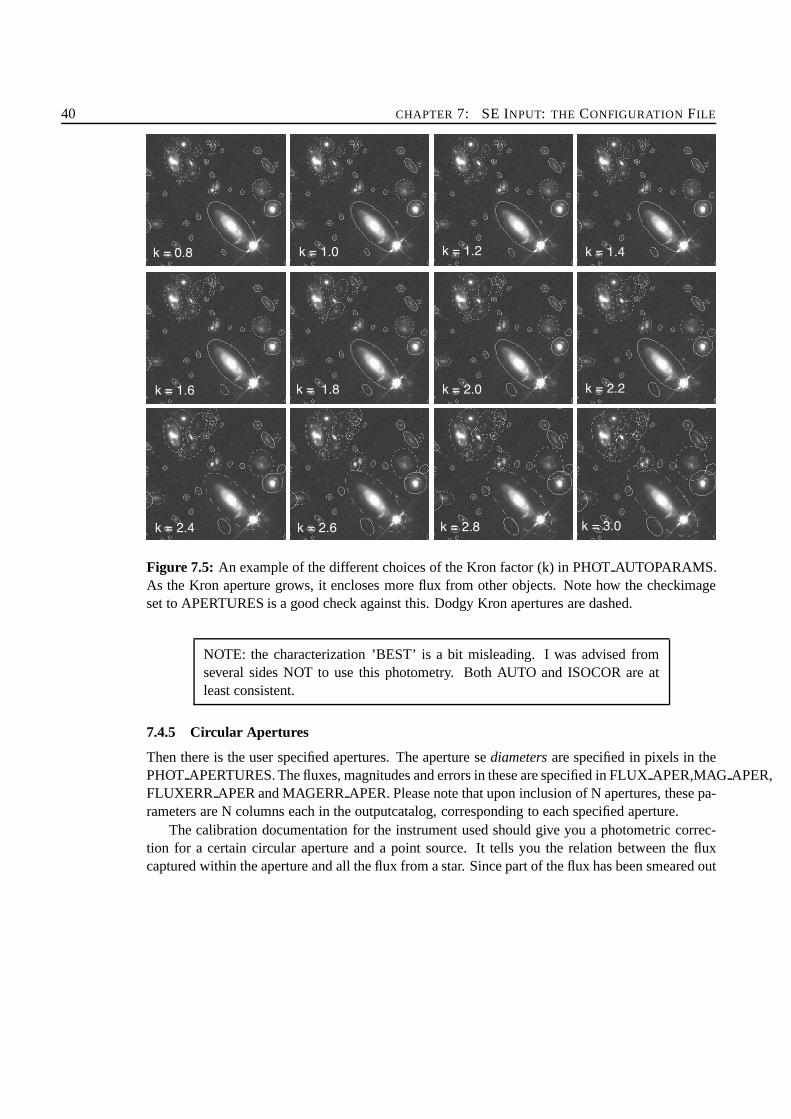
ellipticity η and position angleθ are computed. The major and minor axes of the elliptical apertureare computed to bekr1/ǫ andǫkr1 respectively. PHOTAUTOPARAMS influences directly theestimation. The first is k factor mentioned above and the second is the minimum radius for a Kronellipse.PHOT AUTOAPERS are the minimum aperture diameters for the Kron photometry, estimation andmeasurement. These are circular! These are used in case the radius of the Kron aperture goes belowtheRmin specified in PHOTAUTOPARAMS. The values in the default.sex are probably bestformost applications. A good way to check the setting on PHOTAUTOPARAMS is to generatean ’APERTURES’ check-image and see if the Kron apertures overlap too much with those ofneighboring objects.14
Parameter Default Type DescriptionPHOT AUTOPARAMS - floats (n = 2) MAG AUTO controls:
scaling parameter k ofthe 1st order moment,and minimum Rmin (inunits of A and B).
PHOT AUTOAPERS 0.0,0.0 floats (n = 2) MAG AUTO min-imum (circular)aperture diameters:estimation disk, andmeasurement disk.
Neat trick: The Kron radius was introduced as a accurate flexible aperturethat would capture most of the flux from an object. There is relation betweenthe Kron flux-measurement and the total flux from an object given in Grahamand Driver (2005) depending on the Sersic profile of the galaxy. See for theenclosed fraction table 8.2.
NOTE: In the 2.4.4 version of source extractor provides an alternative very sim-ilar to the AUTO photometry, the PETRO photometry parameters, determinedwithin an aperture defined by the Petrosian radius.
7.4.4 BEST
With all this flexibility, you’d expect the Kron or AUTO photometry to be the best. However it canbe influenced by nearby sources. Therefore there is a fourth option, MAG BEST. This is usuallyequal to AUTO photometry but if the contribution of other sources exceeds 10%, it is ISOCOR.
14Note that the elliptical apertures in figure?? (Source Extractor written in sources? remember? Did you skim overit? you bastard!) are actual Kron apertures for the ’objects’. I cheated however and set PHOTAUTOPARAMS to 1.0so the Kron radii would not be so big.
40 CHAPTER 7: SE INPUT: THE CONFIGURATION FILE
k = 1.0 k = 1.4
k = 1.8
k = 1.2k = 0.8
k = 1.6 k = 2.0 k = 2.2
k = 2.4 k = 2.6 k = 2.8 k = 3.0
Figure 7.5: An example of the different choices of the Kron factor (k) in PHOT AUTOPARAMS.As the Kron aperture grows, it encloses more flux from other objects. Note how the checkimageset to APERTURES is a good check against this. Dodgy Kron apertures are dashed.
NOTE: the characterization ’BEST’ is a bit misleading. I wasadvised fromseveral sides NOT to use this photometry. Both AUTO and ISOCOR are atleast consistent.
7.4.5 Circular Apertures
Then there is the user specified apertures. The aperture sediametersare specified in pixels in thePHOT APERTURES. The fluxes, magnitudes and errors in these are specified in FLUX APER,MAG APER,FLUXERR APER and MAGERRAPER. Please note that upon inclusion of N apertures, these pa-rameters are N columns each in the outputcatalog, corresponding to each specified aperture.
The calibration documentation for the instrument used should give you a photometric correc-tion for a certain circular aperture and a point source. It tells you the relation between the fluxcaptured within the aperture and all the flux from a star. Since part of the flux has been smeared out

TYPICAL RADII 41
of the aperture by the PSF, you need to correct for this. If youhave an extended object, the game isdifferent. Fortunately, there are other apertures15 for this and even a correction for those to accountfor all the flux (but that also depends on the light profile of the galaxy).
One of the geometric output-parameters is the half-light radius. The fraction of total lightwithin this radius is specified in the PHOTFLUXFRAC parameter.
AUTO
APERTURE
ISO
ISOCORR
Figure 7.6: Illustration of the different apertures possible: ISO, ISOCOR, AUTO and APER (userspecified in PHOTAPERTURES
7.5 Typical Radii
There are several output option to describe the typical sizeof an object. Often they also define anaperture that is meant to capture an extended object like a galaxy. These are the input parametersthat are important to them. The FLUXRADIUS has been an output parameter for some time, theKRON and PETROSIAN radii appeared in version 2.4.4 of SE.
15The Kron and Petrosian ones...see sections 8.5.1 and??.

42 CHAPTER 7: SE INPUT: THE CONFIGURATION FILE
7.5.1 Effective Radii
SE has the option to put out radii containing a certain fraction of the light. (outputparameterFLUX RADIUS) The default is 0.5 (the half light radius). PHOTFLUXFRAC 0.2,0.5,0.9 willgive three radii containing 20%, 50% and 90% of the light respectively. The effective radius outputis discussed in section 8.5.3.
Parameter Default Type DescriptionPHOT FLUXFRAC 0.5 floats (n ≤
32)Fraction of FLUXAUTO defining eachelement of the FLUXRADIUS vector.
7.5.2 Kron Radius
The Kron radius is the typical size of the aperture already described in the AUTO photometrysection (section 7.4.3). The whole photometry process is controlled by the PHOTAUTOPARAMSand the definition of the Kron radius is given in section 8.5.1. 16
Parameter Default Type DescriptionPHOT AUTOPARAMS 2.5, 1.5 floats (n=2) MAGAUTO
parameters:(Kron fact),(min radius)
PHOT AUTOAPERS 0.0,0.0 floats (n =2)
MAG AUTO min-imum (circular)aperture diameters:estimation disk, andmeasurement disk.
The Kron fact is the numbe of Kron radii the aperture is set at and the min rad is the minimum Kronradius for which this is done. Otherwise the minimum aperture specified in PHOTAUTOAPERSis used for the photometry.
7.5.3 Petrosian Radius
The Petrosian radius is another defined radius for photometry and this parameter has also only oneinput parameter associated with it, PHOTPETROPARAMS. There is however a defining param-eter for the Petrosian parameter and this is the ratioη. Mostly this is set to 0.2 but occasionallyit is set to 0.5. Unfortunately, it is impossible to change this at this time. See for the completeexpression of the Petrosian radius section 8.5.2.
16Leisurely background reading on the subject does not excistof course but there is? who proposed the radius foraccurate galaxy photometry and more recently (by about 25 years) Graham and Driver (2005) who gives a very niceoverview of the whole photometry within a radius relation. Get it from astro-ph where it’s free though. You’re probablya Graduate student and poor.

TYPICAL RADII 43
Parameter Default Type DescriptionPHOT PETROPARAMS 2.0, 3.5 floats (n=2) MAGPETRO pa-
rameters: (Pet-rosianfact),(min radius)
The Petrosianfact is the number of Petrosian radii the aperture is set at and the minrad is theminimum Petrosian radius for which this is done. Otherwise the minimum radius is used for thephotometry.17
Figure 7.7: In the checkimage there are two radii visible. Good to know: as soon as you specifyeither AUTO (Kron) parameters or PETRO parameters for the output catalog, these apertures willbe drawn in the checkimage (APERTURES). The Petrosian is usually the outer radius.
NOTE: The output parameters asked for and the checkimage with the apertures(checkimagetype = APERTURES) influence each other. If no parameter de-pending on the Kron radius (all the AUTO photometry and KRONRADIUS)is asked for in the parameter file, the Kron radius is NOT drawnin the ckeckim-age.
17If you are having deja-vu all over again, it’s because I copies this directly from the section above...which I’m sureis how the SE code was made as well.

44 CHAPTER 7: SE INPUT: THE CONFIGURATION FILE
7.5.4 Masking Overlapping Objects
Now what if there are two objects overlapping each other? Howto account for the overlapping pix-els? This is handled by the MASKTYPE parameter. NONE means that the counts in the overlapare simply added to the objects total. BLANK sets the overlapping pixels to zero. CORRECT, thedefault, replaces them with their counterparts symmetric to the objects’ center. Best if you leave itat default. I’m just mentioning it out of completeness18
Parameter Default Type DescriptionMASK TYPE CORRECT keyword Method of masking of
neighbors for photom-etry:
NONE no masking,BLANK put detected pixels be-
longing to neighbors tozero,
CORRECT replace by values ofpixels symmetric withrespect to the sourcecenter.
7.6 SE Running
These inputparameter govern the way SE runs, if it should heed flags, how it should heed those, ifand what to put in an outputimage, how much it should comment and how much memory it shoulduse.
7.6.1 Flags
If pixels in your image should be flagged as unreliable or other, SE can use a flag image for thispurpose. This is well described (I think) in the official manual so I copies that section in section??. The internal flags of SE are described in??. If however you have some kind of quality image(such as a Drizzle weight image or a coverage map coming out ofthe MOPEX pipeline), then youcould conceivably convert this to a flag image to be fed to SE here. SE will then combine yourflags (from the flagimage19) with it’s own internal flags20. It also has different ways to combine theflags (specified in FLAGTYPE). If your flags are in ascending order of awfulness (flag =1 meansokay but with a bad pixel, flag=100 means you made this part of the image up...) then you couldgo for MAX or OR option
18NONE might be useful to get the total flux from a large extendedunderlying structure with bright patches and noforeground stars.
19Specified in FLAGIMAGE...ta-dah!20The ones that state that Timmy...I mean your object is too close to the edge etc etc...

SE RUNNING 45
Figure 7.8: Well sometimes flagsare important. Cartoon by S. Bateman, used without any per-mission whatsoever but I don’t make money off this anyway.
Parameter Default Type DescriptionFITS UNSIGNED N boolean Force 16-bit FITS input data to
be interpreted as unsigned inte-gers.
FLAG IMAGE flag.fits strings(n ≤ 4)
File name(s) of the flagimage(s) .
FLAG TYPE OR keyword Combination method for flags onthe same object:
OR arithmetical OR,AND arithmetical AND,MIN minimum of all flag values,MAX maximum of all flag values,MOST most common flag value.
7.6.2 Interpolation
If the data for pixels is missing, SE can interpolate. These parameters regulate the interpolation.Best kept at default. For some, the x and y gaps allowed are a bit wide (16 pixels after all, it isalmost an entire object...). On the other hand, it allowd Sextractor to give you catalogs despite badcolumns. Therefore do not set to zero.

46 CHAPTER 7: SE INPUT: THE CONFIGURATION FILE
Parameter Default Type DescriptionINTERP MAXXLAG 16 integers
(n ≤ 2)Maximum x gap (in pixels) al-lowed in interpolating the inputimage(s).
INTERP MAXYLAG 16 integers(n ≤ 2)
Maximum y gap (in pixels) al-lowed in interpolating the inputimage(s).
INTERP TYPE ALL keywords(n ≤ 2)
Interpolation method from thevariance-map(s) (or weight-map(s)):
NONE no interpolation,VAR ONLY interpolate only the variance-
map (detection threshold),ALL interpolate both the variance-
map and the image itself.
7.6.3 Memory Use
These are the parameters regulating the memory use of SE. To be honest, they are best kept at thevalues in the./sextractor2.2.2/config/default.sexfile. 21 If you have the FLAGS output, then youcan check if there were any memory problems in the SE run. If so, this can be very bad for thecompleteness of your catalog (it isn’t probably). In that case you might want to fiddle with theMEMORY BUFSIZE and rerun.
Parameter Default Type DescriptionMEMORY BUFSIZE - integer Number of scanlines in the im-
agebuffer. Multiply by 4 theframe width to get equivalentmemory space in bytes.
MEMORY OBJSTACK - integer Maximum number of objectsthat the objectstack can con-tain. Multiply by 300 to getequivalent memory space inbytes.
MEMORY PIXSTACK - integer Maximum number of pixelsthat the pixel-stack can con-tain. Multiply by 16 to 32 toget equivalent memory space inbytes.
21SE was programmed to do large images, even with limited memory and computing power. The only reason tochange these defaults is when you get something of a stack overflow.
SE OUTPUT SETTINGS 47
7.6.4 Neural Network
There is to date only one neural network file and it’s in the same directory (default.nnw) as the otherconfig files. Use this one. Don’t edit it. I think the original idea was to have specialized neuralnetwork files for different types of instruments but it turnsout it’s much easier to run something ona SE catalog.
Parameter Default Type DescriptionSTARNNW NAME - string Name of the file containing
the neural network weights forstar/galaxy separation.
7.6.5 Comments
The VERBOSETYPE parameter regulates the amount of comments printed on the command line.It could possibly be instructive to run it with FULL once in a while. the descriptions are not veryhelpful but then again you only want to use QUIET if SE is part of some kind of pipeline and FULLif something is off and you can’t figure out what.
Parameter Default Type DescriptionVERBOSETYPE NORMAL
keyword How much SExtractor com-ments its operations:
QUIET run silently,NORMAL display warnings and limited
info concerning the work inprogress,
EXTRA WARNINGSlike NORMAL, plus a fewmore warnings if necessary,
FULL display a more complete infor-mation and the principal pa-rameters of all the objects ex-tracted.
7.7 SE output settings
SE has two types of output. The catalogs with a whole range of characteristics of each of thedetected objects and outputs which allow you to compare SE estimates of background, aperturesand objects with the real data.
7.7.1 Catalog
The catalog is what you are running SE for! So in CATALOGNAME , you specify the name ofthe output catalog. Again it’s probably a good idea to start straight away with a naming convention.(a .cat extension for instance!)

48 CHAPTER 7: SE INPUT: THE CONFIGURATION FILE
The CATALOG TYPE enables you to specify the type of outputcatalog. Personally I prefer theASCII HEAD, as it allows me to read it in just about anywhere and still tells me which parametersare listed. The nice thing about the fits catalog is that all the input parameter settings are saved inthe header.
NOTE: the fits option can’t handle array outputinformation such asMAG APER,FLUX RADIUS if more than one value!
22
The ASCII SKYCAT option for instance does not list all the parameters before the actualcatalog (like ASCIIHEAD) but puts the name of the output parameter on top of the column inquestion.
And which parameters to list is specified in the file given to PARAMETERSNAME.Parameter Default Type DescriptionCATALOG NAME - string Name of the output catalog. If
the name “STDOUT” is givenand CATALOG TYPE is set toASCII, ASCII HEAD, or ASCIISKYCAT, the catalog will bepiped to the standard output (std-out)
CATALOG TYPE - keyword Format of output catalog:ASCII ASCII table; the simplest, but
space and time consuming,ASCII HEAD
as ASCII, preceded by a headercontaining information about thecontent,
ASCII SKYCATSkyCat ASCII format (WCS co-ordinates required),
FITS 1.0 FITS format as in SExtractor 1,FITS LDAC
FITS “LDAC” format (the origi-nal image header is copied).
PARAMETERSNAME - string The name of the file containingthe list of parameters that will becomputed and put in the catalogfor each object.
22I have this on Ed’s authority. I have NO idea how to display a fits table. Since there have been quite a number ofupdates, I think thismaybe fixed by now. Not very helpful I know.

SE OUTPUT SETTINGS 49
7.7.2 ASSOC parameters
These are the parameters dealing with crosscorrolating twocatalogs: a catalog of targets and theoutput catalog. (The target catalog is given in ASSOCNAME, the output one is created as SEruns). The cross correlation is controlled by two parameter: ASSOCRADIUS and ASSOCTYPE,the first governing the search radius and latter which objects gets selected if there are multiplecandidates near the positions. The numbers of the columns intarget catalog which contain thex,y positions of the objects need to be in ASSOCPARAMS. A third column here can be usedas weight. So you can crosscorellate catalogs weighted withmagnitude but also with anotherparameter such as FWHM or no of pixels. Useful it you’re crosscorellating between catalogs ofdifferent filters. Some of the columns in target catalog (with the to-be-crosscorellated objects) canbe put into the second output catalog. These columns are specified in ASSOCDATA and end upin the VECTORASSOC.
NOTE: ASSOC works only with pixel positions (NOT RA and DEC!)
NOTE: Be aware of shifts and rotation between images when crosscorrellatingtwo catalogs. Find shifts beween images with imcentroid in IRAF for instance.
NOTE: ASSOC will appear not to work if you don’t ask for a ASSOCoutputparameter in the parameter file. Your catalog better containeither the VEC-TOR ASSOC or the NUMBERASSOC output, otherwise SE simply runs andoutputsall objects it has detected, not just the crosscorellated ones23.
Emmanuel sez: Unfortunately, SExtractor can only handle floating point num-bers in ASSOC files. In fact, ASSOC file may have comment lines (like an SEheader) but no tab spacing either. Your best bet is just a listof x and y positions(with possibly a weight) separated with white spaces and nothing else.

50 CHAPTER 7: SE INPUT: THE CONFIGURATION FILE
Parameter Default Type DescriptionASSOCNAME sky.list string Name of the ASSOC
ASCII file.ASSOCPARAMS 2,3,4 integers (n ≤
2, n ≤ 3)Nos of the columnsin the ASSOC filethat will be usedas coordinates andweight for cross-matching.
ASSOCRADIUS 2.0 float Search radius (in pix-els) for ASSOC.
ASSOCTYPE MAG SUM keyword Method for cross-matching in ASSOC:
FIRST keep values corre-sponding to the firstmatch found,
NEAREST values correspondingto the nearest matchfound,
MEAN weighted-averagevalues,
MAG MEAN exponentiallyweighted averagevalues,
SUM sum values,MAG SUM exponentially sum
values,MIN keep values cor-
responding to thematch with minimumweight,
MAX keep values cor-responding to thematch with maxi-mum weight.

SE OUTPUT SETTINGS 51
Parameter Default Type DescriptionASSOCSELECTYPE MATCHED keyword What sources are
printed in the out-putcatalog in case ofASSOC:
ALL all detections,MATCHED only matched detec-
tions,-MATCHED only detections that
were not matched.ASSOCDATA 2,3,4 integers
(n ≤ 32)Numbers of thecolumns in the AS-SOC file that will becopied to the catalogout-put.
NOTE: ASSOC does not work as long as you do not ask for the ASSOCoutputin the parameter file (specified in PARAMETERSNAME.). So don’t forgetto ask for VECTORASSOC or NUMBERASSOC in the parameter file orotherwise all the detections are reported.
7.7.3 The Check-images
SE can output some of the maps used in intermediate steps. Thenames for the output fits filesare specified in CHECKIMAGENAME. Keep a convention like your filebackground.fits or yourfile bgr.fits. A list of up to 16 can be given (separated by a comma).24
The type of output files you want is defined in CHECKIMAGETYPE. As you can see, mostof these have to do with the background estimation. Notable exceptions are the APERTURES andSEGMENTATION options. APERTURES is a good diagnostic on whether or not your threshold isright and the SEGMENTATION will show you if the objects are broken up too much or not. Loadthe original and this segmentation image into saotng and compare.
SEGMENTATION has another useful feature, the number in the catalog is given as the valueto the isoarea in this image. Good for figuring out what is whatfrom the catalogs. Also, thesegmentation image is used as input for follow-up fit programs of extended sources (GALFIT andGIM2D).
24Oddly enough, this more than covers all your options, including NONE for the type of checkimage.

52 CHAPTER 7: SE INPUT: THE CONFIGURATION FILE
NOTE: APERTURES checkimage shows the apertures you’ve asked for. So ifyou ask for a MAGAUTO, the Kron radius will be drawn on the checkimage.If NO Kron derived parameter is put into the catalog, the Kronradius willalso not be drawn on the APERTURES checkimage. Same for the APER andPETRO apertures.
Parameter Default Type DescriptionCHECKIMAGE NAME check.fits strings (n ≤
16)File name for eachcheck-image .

SE OUTPUT SETTINGS 53
Parameter Type DescriptionCHECKIMAGE TYPE keywords (n ≤ 16) Type of information
to put in the check-images :
NONE no check-image,IDENTICAL identical to input im-
age (useful for convert-ing formats),
BACKGROUND full-resolution interpo-lated background map,
BACKGROUND RMS full-resolution interpo-lated background noisemap,
MINIBACKGROUND low-resolution back-ground map,
MINIBACK RMS low-resolution back-ground noise map,
-BACKGROUND background-subtractedimage,
FILTERED background-subtractedfiltered image (requiresFILTER = Y),
OBJECTS detected objects,-OBJECTS background-subtracted
image with detectedobjects blanked,
APERTURES MAG APER and MAGAUTO integration lim-its,
SEGMENTATION display patches corre-sponding to pixels at-tributed to each object.

54 CHAPTER 7: SE INPUT: THE CONFIGURATION FILE
Original Background
’Filtered’ Objects
Segementation Apertures
Figure 7.9: Illustration of the different checkimages possible. The original inputimage, the BACK-GROUND image, the FILTERED image, the OBJECTS image, the SEGMENTATION image andthe APERTURES image. the contrast of the BACKGROUND image has been exaggerated.

Chapter 8
Output Parameters
The catalogs with output parameters is what the whole exercise is all about!1 You can finally startconstructing your Hertzsprung-Russel diagrams or lensingshear fields or whatever. The param-eters you want in your catalogs should be listed in the file yougave to PARAMETERSNAME.Unless you keep using the same file for this, I really recommend using ASCIIHEAD type catalogs2 The output catalogs will have a nice header with a list of all the parameters.
Parameters in the SE outputcatalog can be divided into geometric parameters ,photometricparameters, astrometric parameters and fitted parameters.3 Geometric parameters will tell youwhat shape the object is in (basically how the light of the object is distributed over the pixels ofthat object) and the photometric parameters tell you simplyhow much light there is. Astrometricparameters give the position of the object in the image, be itin pixels or other coordinates.4 Fittedparameters are calculated from fitting for instance a PSF to the data of the object. Most of theseare still being developed and do not work yet.5
There are a few that do not fall in any of these convenient categories; the catalog number, theflag parameters and the parameters associated with crosscorrellating catalogs.
Name description unitNUMBER Running object number -FLAGS Extraction flags -IMAFLAGS ISO FLAG-image flags OR’ed over the iso. profile -NIMAFLAGS ISO # flagged pixels entering IMAFLAGSISO -
1Well that and the check-images perhaps.2By setting the parameter CATALOGTYPE to ASCII HEAD in the configuration file.3Just kidding, SE does not fit anything yet. It’s so fast for a reason.4There has been some improvement here as well. The now nearly ubiquitous World Coordinate System WCS is also
used.5Meaning, I’ve tried but have not gotten them to work yet...Ifyou have, let me know.

56 CHAPTER 8: OUTPUT PARAMETERS
8.1 Photometric Parameters
Photometric parameters are either flux or magnitude determined by SE. However SE has five dif-ferent ways of determining these; isophotal, isophotal-corrected, automatic, best estimate and aper-ture. These are discussed in the Photometry section in the input chapter (section 7.4). To recap:
ISO Photometry derived from the counts above the thresholdminus the background (see also section 7.4.1).
ISOCOR ISO photometry, corrected for loss as a Gaussian profile(see also section 7.4.2).
AUTO Photometry from the Kron flexible elliptical aperture.?(see also section 7.4.3)
BEST Choice between AUTO and ISOCOR. AUTO, exceptwhen influence from neighbors is more than 10%. (seealso section 7.4.4)
APER Photometry from circular, user specified(PHOT APERTURES in the config file), apertures.(see also section 7.4.5)
PETRO Photometry from the Petrosian aperture, very similartothe Kron aperture. (see also section??)
PROFILE the weighted photometry using the ’filtered’ image for theweight.
There are two other photometric parameters of interest: MUMAX, the surface brightness ofthe brightest pixel and the MUTHRESHOLD, the the surface brightness corresponding to thethreshold. This last parameter is good to inspect if the threshold is set with respect to the back-ground RMS. The value of the Background at the position of theobject is often also interesting toknow. Especially when deciding whether or not to switch between GLOBAL and LOCAL in theBACK TYPE parameter (see section 7.2).
The Petrosian aperture is a recent addition to SE (since v2.4.4 as far as I know) and it is verysimilat to the Kron radius. The apreture has a different radius (a Petrosain vs. a Kron one.).However the position angle and the ellipticity are the same as the Kron aperture. The Petrosianradius is usually bigger than the Kron one. See also section 7.5.2, 8.5.1 and 7.4.3 for Kron aperturestuff and see section 7.5.3 and 8.5.2 for more on the Petrosian radius.
NOTE: oh and I’ll say it again...the ”BEST” photometry is a misnomer. Ratheruse something that is consistent across your image.
NOTE: For a color (Great Brittain and Canada: colour) measurement, the ISOand APER options are good, especially when run in dual mode since you’llknow the apertures are the same. The other apertures may be too inclusive incrowded fields.

PHOTOMETRIC PARAMETERS 57
AUTO
APERTURE
ISO
ISOCORR
Figure 8.1: Illustration of the different apertures possible; ISO, ISOCOR, AUTO and APER (userspecified in PHOTAPERTURES)
Name description unitFLUX ISO Isophotal flux countFLUXERR ISO RMS error for isophotal flux countMAG ISO Isophotal magnitude magMAGERR ISO RMS error for isophotal magnitude mag
FLUX ISOCOR Corrected isophotal flux countFLUXERR ISOCOR RMS error for corrected isophotal flux countMAG ISOCOR Corrected isophotal magnitude magMAGERR ISOCOR RMS error for corrected isophotal magnitude mag
FLUX AUTO Flux within a Kron-like elliptical aperture countFLUXERR AUTO RMS error for AUTO flux countMAG AUTO Kron-like elliptical aperture magnitude magMAGERR AUTO RMS error for AUTO magnitude mag
FLUX BEST Best of FLUXAUTO and FLUX ISOCOR countFLUXERR BEST RMS error for BEST flux countMAG BEST Best of MAGAUTO and MAG ISOCOR magMAGERR BEST RMS error for MAGBEST mag
FLUX APER Flux vector within fixed circular aperture(s) countFLUXERR APER RMS error vector for aperture flux(es) countMAG APER Fixed aperture magnitude vector magMAGERR APER RMS error vector for fixed aperture mag. mag
FLUX PETRO Flux within a Petrosian-like elliptical aper-ture
count
FLUXERR PETRO RMS error for PETROsian flux countMAG PETRO Petrosian-like elliptical aperture magnitude magMAGERR PETRO RMS error for PETROsian magnitude mag
58 CHAPTER 8: OUTPUT PARAMETERS
8.2 Profile
The profile option for photometry is not a much used one. The idea is to weigh the fluxes withthe values in the filtered (smoothed) image (see section 7.3.2 for the options here). in general,smoothing correlates the noise in an image and broadens profiles. By weighting with the smoothedprofile, you give extra weight to the brightest pixels (as opposed to counting all the flux equally).
NOTE: the PROFILE option seems to be a fix for when you think youincludetoo much noise in the flux measurements (i.e. the detection threshold is toolow, background too funky or something...) Use with some caution.
And remember kids: the ellipticity and everything is derived from the ’filtered’(i.e. smoothed) image. The PROFILE option in this context might be a goodway to check up how much different things are between the smoothed and theoriginal image.
Name description unitFLUX PROFILE Flux weighted by the FILTERed profile countFLUXERR PROFILE RMS error for PROFILE flux countMAG PROFILE Magnitude weighted by the FILTERed pro-
filemag
MAGERR PROFILE RMS error for MAGPROFILE mag
Name description unitMU THRESHOLD Detection threshold above back-
groundmag× arcsec−2
MU MAX Peak surface brightness above back-ground
mag× arcsec−2
BACKGROUND Background at centroid position countsTHRESHOLD Detection threshold above back-
groundcounts
8.3 Astrometric Parameters
The astrometric parameters are simple enough; they tell youwhere the object is located. Howeverwhich pixel do you take for the center of the objects? The maximum flux pixel? Or the barycenter?6 Do you want it in RA and DEC or in prosaic pixels? All of these you should be able to specify
6The Barycenter is the flux-weighted average position. the first moment, SE computes all the second moments aswell, see the geometric parameters section and chapter 9 in the manual v2.1.3.

ASTROMETRICPARAMETERS 59
from the list below.
NOTE: the x and y positions (with the exception of ’peak’ values) are thebarycenters of objects; the weighted mean position.
The definition for the barycenter of an object is:
X = x =ΣIixi
ΣIi
Y = y =ΣIiyi
ΣIi
This is the first order moment of the object.7 The minima and maximum x and y pixelvalues almostspeak for themselves. These are the most extreme values for xand y that are still within the object.Handy if you want to make postage stamps of some of your objects from the fits file. The PEAKvalues are the x,y and ra and dec values for the position of thebrightest pixel. The value for the fluxand surface brightness of that pixel can be found in output-parameters FLUXMAX and MU MAXrespectively. The difference between the position of the brightest pixel and the (bary) center ofan object might help you identify blended objects. If they differ much, than you’ve got somethinglobsided.
NOTE: all thexi andIi values in these formulae are the values from the pix-els identified in the segmentation map as belonging to the object. It can beinfluenced by detection thresholds and segmentation settings.
NOTE: The origin for XIMAGE etc is pixel 1,1. SO The first pixel in the leftbottom corner of the FITS image is number 1,1 and not 0,0.
7Yes this is straight from the sextractor manual. All this stuff is quite complete in the manual v2.1.3 and above. Isthere a problem?
60 CHAPTER 8: OUTPUT PARAMETERS
Name description unitXMIN IMAGE Minimum x-coordinate among detected pix-
elspixel
YMIN IMAGE Minimum y-coordinate among detected pix-els
pixel
XMAX IMAGE Maximum x-coordinate among detected pix-els
pixel
YMAX IMAGE Maximum y-coordinate among detected pix-els
pixel
YPEAK IMAGE y-coordinate of the brightest pixel pixelXPEAK WORLD World-x coordinate of the brightest pixel degYPEAK WORLD World-y coordinate of the brightest pixel degALPHAPEAK SKY Right ascension of brightest pix (native) degDELTAPEAK SKY Declination of brightest pix (native) degALPHAPEAK J2000 Right ascension of brightest pix (J2000) degDELTAPEAK J2000 Declination of brightest pix (J2000) degALPHAPEAK B1950 Right ascension of brightest pix (B1950) degDELTAPEAK B1950 Declination of brightest pix (B1950) degX IMAGE Object position along x pixelY IMAGE Object position along y pixelX IMAGE DBL Object position along x (double precision) pixelY IMAGE DBL Object position along y (double precision) pixelX WORLD Barycenter position along world x axis degY WORLD Barycenter position along world y axis degX MAMA Barycenter position along MAMA x axis m−6
Y MAMA Barycenter position along MAMA y axis m−6
ALPHA SKY Right ascension of barycenter (native) degDELTA SKY Declination of barycenter (native) degALPHA J2000 Right ascension of barycenter (J2000) degDELTA J2000 Declination of barycenter (J2000) degALPHA B1950 Right ascension of barycenter (B1950) degDELTA B1950 Declination of barycenter (B1950) deg
According to the v2.3 manual of SE, FITS header-informationis used for the WORLD coor-dinates. World Coordinates System (WCS) is often what you use to line up different images fromdifferent observatories in ds9 (that’s what I do...).No idea what the MAMA axis is.
8.4 Geometric Parameters
Geometric parameters describe the shape and size of the object. SE computes the moments ofan object and determines elliptical parameters from these.Both the moments and the elliptical

GEOMETRIC PARAMETERS 61
parameters and derivatives from these can be included in theoutput. These parameters are treatedmuch more extensive in chapter 9 of the manual (version 2.1.3).
8.4.1 Moments
The first order moments are the barycenters of course but the second order moments can also begiven (see section 9.1.4 in the manual v2.1.3):
X2 = x2 =ΣIix
2i
ΣIi− x2 (8.1)
Y 2 = y2 =ΣIiy
2i
ΣIi− y2 (8.2)
XY = xy =ΣIixiyi
ΣIi− xy (8.3)
Name description unitX2 IMAGE Variance along x pixel2
Y2 IMAGE Variance of position along y pixel2
XY IMAGE Covariance of position between x and y pixel2
X2 WORLD Variance of position along X-WORLD (alpha) deg2
Y2 WORLD Variance of position along Y-WORLD (delta) deg2
XY WORLD Covariance of position X-WORLD/Y-WORLD deg2
NOTE: By adding ERR+parameter, the error can be obtained as well. (e.g.ERRX2 IMAGE)
8.4.2 Ellipse parameters
From these moments, the position angle, the minor and major axis of an ellipse can be derives(section 9.1.5 in the manual v2.3) and also a second way of describing this ellipse is given (sec9.1.6). The official manual gives the whole derivation of these parameters but since we want aquick result I’ll cut it down some.
NOTE: All these elliptical parameters are computed in the SMOOTHED image.So If you have used a smoothing kernel in the input, then the ELLIPTICITY isalso of a smoothed object.8
62 CHAPTER 8: OUTPUT PARAMETERS
Minor and Major Axes
The following definitions for thesecomputed parameters are: (see for the derivation the v2.3manual page 28)
A2 =x2 + x2
2+
√
√
√
√
(
x2 − y2
2
)2
+ xy2 (8.4)
B2 =x2 + x2
2−
√
√
√
√
(
x2 − y2
2
)2
+ xy2 (8.5)
These are illustrated in figure 8.2. Not also that the Petrosian and Kron radii (section 8.5.2 and8.5.1) are expressed in the same units as those used for the A and B values.
Figure 8.2: Illustration of the Kron radius.x andy are the computed center in of the object.
Name description unitA IMAGE Profile RMS along major axis pixelB IMAGE Profile RMS along minor axis pixelTHETA IMAGE Position angle (CCW/x)counterclockwise!!!9 degA WORLD Profile RMS along major axis (world units) degB WORLD Profile RMS along minor axis (world units) deg
Errors can be obtained using ERR+parameter in the paramfile.

GEOMETRIC PARAMETERS 63
Position Angle
This is the rotation of the major axis with respect to NAXIS1 (x-axis...) counterclockwise. The def-inition of the position angle is different (pa is with respect to North.) However the conversion canobviously be done and the Position Angle (PA) is given in other THETA parameters (SKY, B1950and J2000). This can be very useful if you’re looking for slit-positions for your spectrograph.
Name description unitTHETA WORLD Position angle (CCW/world-x) degTHETA SKY Position angle (east of north) (native) degTHETA J2000 Position angle (east of north) (J2000) degTHETA B1950 Position angle (east of north) (B1950) deg
Errors can be obtained using ERR+parameter in the paramfile.
The Other Ellipse parametrisation
So the manual also gives another parametrisation of the elliptical aperture. I have not used theseparameters. I have no idea what to do with them. Maybe you do. In figure 8.2, the relation betweenthese parameters and the moments is given.
Name description unitCXX IMAGE Cxx object ellipse parameter pixel−2
CYY IMAGE Cyy object ellipse parameter pixel−2
CXY IMAGE Cxy object ellipse parameter pixel−2
CXX WORLD Cxx object ellipse parameter (WORLD units) deg−2
CYY WORLD Cyy object ellipse parameter (WORLD units) deg−2
CXY WORLD Cxy object ellipse parameter (WORLD units) deg−2
Errors can be obtained using ERR+parameter in the paramfile.
Ellipticity and Elongation
How stretched the object is can be parameterised with weither the Ellipticity or the Elongationparameters, both of which are simply computed from the minorand major axes.
ELONGATION =A
B(8.6)
ELLIPTICITY = 1 −B
A= 1 −
1
ELONGATION(8.7)
Name description unitELONGATION A IMAGE/B IMAGEELLIPTICITY 1 - B IMAGE/A IMAGE
64 CHAPTER 8: OUTPUT PARAMETERS
NOTE: If you have FILTERED the image for detection then your ellipticity andelongation values will be moreround than the actual object.
Only the ELONGATION and the ELLIPTICITY parameters do not come with a error. Notethat there is an extensive discussion of these in section 9.1.8 of the manual.10
8.4.3 Area Parameters
This can be done by the parameters describing the isophotes as fitted by SE or the conclusion ofthe neural network classification. To get an idea of the size of an object, reasonably independent ofthe brightness, the FWHM or the FLUXRADIUS
SE divides an object up into 7 isophotes above the ANALYSISTHRESH. The areas above theisophotes is fed to the neural network. These can be put into the catalog with the ISOn parameters.
Name description unitISOAREA WORLD Isophotal area above Analysis threshold deg2
ISOAREAF WORLD Isophotal area (filtered) above Detectionthreshold
deg2
ISO0 Isophotal area at level 0 pixel2
ISO1 Isophotal area at level 1 pixel2
ISO2 Isophotal area at level 2 pixel2
ISO3 Isophotal area at level 3 pixel2
ISO4 Isophotal area at level 4 pixel2
ISO5 Isophotal area at level 5 pixel2
ISO6 Isophotal area at level 6 pixel2
ISO7 Isophotal area at level 7 pixel2
8.4.4 Full-Width Half Max
Assuming a Gaussian profile for the object, a Full-Width at Half Maximum can be computed. Noobject is a Gaussian -especially in the wings- but this does give you a reasonable idea of the PSFwidth in the case of a star for instance. It’s a useful thing tohave.
Name description unitFWHM WORLD FWHM assuming a Gaussian core pixelFWHM WORLD FWHM assuming a Gaussian core degVIGNET Pixel data around detection countVIGNET SHIFT Pixel data around detection corrected for
shiftcount
THRESHOLDMAX Maximum threshold possible for detection count
10I’d be saying the exact same thing and typing in that many functions is a pain, even in LaTeX.
RADII 65
8.5 Radii
Indicators for the size of objects are multiple and SE can provide a lot of them if so desired.Especially for extended source several schemes have been developed to define an aperture to deter-mine the total flux and characterize the size of an object. In the section 7.5.2, 8.4.2 and 7.4.3, theKron aperture and the various associated parameters were already discussed. The KRONRADIUSoutput parameter is the indicator of size of the KRON aperture. Alternatively, there is the PET-ROSIAN RADIUS (since SE v2.4.4). Both of these are expressed in multiples of major axis B.
Table 8.1: Radii nomenclatureRadius symbol Description
Kron R1 The typical size of the flexible aperture -computed from moments-defined by?.
Petrosain Rp The radius at which the surface brightness of the isophote isη times the average surfacebrightness within this isophote.
Effective Re The radius containing 50% of the total flux of an object.Half-light same radius.Typical Rt or h The scale in the exponential diskI = I0 exp(−R/Rt)deVaucouleur R25 The radius at which the B-band isophote is
25 mag arcsec−2. This is a common Radius asit is listed in the third reference catalog (RC3)
8.5.1 Kron radius
? defined the KRON radius to get 90% of an objects light as follows:
R1(R) =2π∫ R0 I(x)x2dx
2π∫ R0 I(x)xdx
(8.8)
According Graham and Driver (2005), the orginal SE publication has changed the definition abit. Bertin and Arnouts (1996) define the Kron radius as:
R1 =ΣR I(R)
ΣI(R)(8.9)
over the two dimentional aperture and not for a lightprofile (which was Kron’s original idea.) Inthe case of a lightprofile, the Kron-radius should be according to Kron’s original definition:
R1 =ΣR2 I(R)
ΣR I(R)(8.10)

66 CHAPTER 8: OUTPUT PARAMETERS
So the Kron radius coming out of SE is maybe not a proper one butwe’re using this as theestimate anyway. And if you are interested in galaxy profiles, here is a neat trick to relate this Kronradius to theeffectiveradius (Re), the radius that encloses half the object’s light.11
R1(x, n) =Re
bn
γ(3n, x)
γ(2n, x)(8.11)
In which x = b(R/Re)1/n andγ is the incomplete gamma function12. This is all too much of a
headache so Graham and Driver (2005) also give a nice table converting these radii depending onSersic profile index (copied in table 8.2).
Table 8.2: Theoretical Kron Radii and Magnitudes from Graham and Driver (2005)Sersic n R1 L(< 2R1) L(< 2.5R1)
(Re) % %0.5 1.06 95.7 99.31.0 1.19 90.8 96.02.0 1.48 87.5 92.23.0 1.84 86.9 90.84.0 2.29 87.0 90.45.0 2.84 87.5 90.56.0 3.53 88.1 90.77.0 4.38 88.7 91.08.0 5.44 89.3 91.49.0 6.76 90.0 91.910.0 8.39 90.6 92.3
Name description unitKRON RADIUS Kron radius in units of A or B -
And remember that the KRON flux measurements can be found in the AUTO output-parameters.13
8.5.2 Petrosian radius
Petrosian (1976) defined a point in the radial light profile atwhich the isophote at that radius was acertain fraction of the average surface brightness within that radius.
η(R) =2π∫ R0 I(R′)R′dR′
πR2I(R)=
〈I〉RI(R)
(8.12)
11All these radii to characterize galaxy profiles can be a tad confusing. See table 8.1 for the definitions of all.12Oh Gamma function, is there something you’re not useful for?13Named differently for your inconvenience. Please rememberthat a lot of SE stuff got tacked on later which explains
the funky naming ’convention’.

OBJECT CLASSIFICATION 67
where the parameterη is the fraction. This is often either 0.2 or 0.5 with 0.2 the most commonlyused. I am pretty sure the 0.2 value is used in SE.
NOTE: Theη cannot be changed using some input-parameter. Bummer.
There is an input parameter associated with this in source extractor ( PHOTPETROPARAMS)where the first input defines the number of Petrosian radii forthe magnitude and the second theminimum radius. The following output parameters are associated with the Petrosian radius:
Name description unitPETRORADIUS Petrosian apertures in units of A or B -FLUX PETRO Flux within Petrosian radius elliptical aper-
turecount
FLUX PETRO Flux within Petrosian radius elliptical aper-ture
count
FLUXERR PETRO RMS error for PETRO flux countMAG PETRO magnitude within theN × Rp magMAGERR PETRO RMS error for the MAGPETRO magnitude mag
More on the Petrosian radius can be found in Graham and Driver(2005) and Graham et al. (2005).
8.5.3 Effective radius
The effective radius is the term commonly used to define the point in a light profile within whichencloses half the flux from an object. In the case of SE, several radii can be defined (input parameterPHOT FLUXFRAC). PHOTFLUXFRAC 0.5 is the effective radius (or SE’s determinationof it.)
Name description unitFLUX RADIUS Radius enclosing a specified fraction of the
fluxpixel.
With the photometry in the APER parameters.So here is another trick. If you’s want an estimate of the Sersic profile index n, you could use
the ratio between the FLUXRADIUS with PHOTFLUXFRAC set to 0.5 and the KRONRADIUSin your catalog. Of course you would need to run some follow-up program to properly determinethe actual index from a fit, but that is what SE is all about.14
8.6 Object classification
This is a section completely devoted to the CLASSSTAR parameter; SE’s classification of theobjects on the basis of a Neural Network Output.15
14A quick and possibly dirty first look, quick sample selectionetc...15If you DO want to know more on Neural Networks and how they are used for complex issues such as object
classifiacation, I found the book ’An introduction to NeuralNetworks’ by Kevin Gurney very useful.

68 CHAPTER 8: OUTPUT PARAMETERS
Name description unitCLASS STAR S/G classifier output none
It can have a value between 0 (galaxy, more to the point: non-star) and 1 (star).
8.6.1 Input Dependency
Fortunately, you do not need to understand Neural Networks to use this but there are several inputparameters which are directly linked to the CLASSSTAR parameter:
• PIXEL SCALE: Pixel size in arcsec. (for surface brightness parameters, FWHM and star/galaxy separation only).
• SEEINGFWHM: FWHM of stellar images in arcsec. This quantity is usedonly for theneural network star/galaxy separation as expressed in theCLASS STAR output.
These are obvious. The NNW has to take in account the scale andblurring of the objects beforejudgment. These are inputparameters of the NNW. The ratio between the two is something you canplay around with. (remember that SE does not use the pixelsscale for anything else...) But thereare parameters where it depend more indirectly on:
• BACK SIZE Size, or Width, Height (in pixels) of a background mesh.
• THRESHTYPE Meaning of the DETECT THRESH and ANALYSISTHRESH parameters:
– RELATIVE scaling factor to the background RMS.
– ABSOLUTE absolute level (in ADUs or in surface brightness).
• ANALYSIS THRESH Threshold (in surface brightness) at which CLASS STAR and FWHMoperate.
– 1 argument: relative to Background RMS.
– 2 arguments: mu (magarcsec−2 ), Zero-point (mag).
Obviously the brightness level from which objects are considered influence heavily the classi-fication. If only the top levels are considered, even clear galaxies might be classified as stars (thedisk lies below the threshold) and if the threshold is too low, random noise can pass itself off as afaint galaxy.
NOTE: if the threshold is relative to the RMS, the BACKSIZE is VERY im-portant for the CLASSSTAR

OBJECT CLASSIFICATION 69
• DEBLEND MINCONT Minimum contrast parameter for de-blending.
• DEBLEND NTHRESH Number of deblending sub-thresholds.
NOTE! if deblending is too course, a clump of stars can becomea ’galaxy’.
NOTE! And if deblending is too picky, a single galaxy might bechopped upinto several objects.
There is no single remedy but a DEBLENDNTHRESH of 32 and a DEBLENDMINCONTof order 0.01 are a good place to start.
HMMMM: If the ANALYSIS THRESH is different from the DE-TECT THRESH, the objects are NOT detected again. So carefull withmakingthese different.
8.6.2 Reliability
This section is one big note of caution. The NNW classification by SE is NOT perfect and willbreak down at the lower magnitude end. Unfortunately it doesnot give another value for unreliableclassification (42 for instance) but assigns a random value between 0 and 1. (see figure 8.3)

70 CHAPTER 8: OUTPUT PARAMETERS
Figure 8.3: The dependence of CLASSSTAR on the luminosity of objects. The reliability clearlydisappears at the lower end.

ASSOCOUTPUT 71
8.7 ASSOC output
These are the two output parameters associated with cross correlating catalogs. If you have speci-fied a ASSOC file and the manner of cross-identification (see the input parameters in section 6.3).Be sure to specify one of these as otherwise there will be NO crosscorellation and the SE catalogwill contain just as many entries as without the ASSOC parameters specified.16 The column in theASSOCNAME catalog, specified in ASSOCDATA are given in the VECTORASSOC
Name description unitVECTOR ASSOC ASSOCiated parameter vectorNUMBER ASSOC Number of ASSOCiated IDs
8.8 Flags
How to steal a country through the cunning use of flags:Brittain: I claim India for Brittain!India: You can’t claim us! There’s 300 million of us already living here!Brittain: Do you have a flag? No flag, no country.–adapted from Eddie Izzard.
This section is the one in the official manual with some annotations of mine.17
A set of both internal and external flags is accessible for each object. Internal flags are producedby the various detection and measurement processes within SExtractor; they tell for instance if anobject is saturated or has been truncated at the edge of the image.
External flags come from flag-maps: these are images with the same size as the one whereobjects are detected, where integer numbers can be used to flag some pixels (for instance, bador noisy pixels). These types of images are becoming quite common data-products of reductionpipelines of current space missions like the Hubble or Spitzer telescopes or the grand surveys suchas SLOAN.
Different combinations of flags can be applied within the isophotal area that defines each object,to produce a unique value that will be written to the catalog.
8.8.1 Internal Flags
The internal flags are always computed and the default.paramfile lists them. Clearly They areaccessible through the FLAGS catalog parameter, which is a short integer. FLAGS contains, codedin decimal, all the extraction flags as a sum of powers of 2:
1 The object has neighbours, bright and close enough to signicantly bias the MAG AUTOphotometry18, or bad pixels (more than 10% of the integrated area affected).
16I will NOT tell anyone how long it took me to figure THAT one out...17I steal the official manual’s prose from it with reckless abandon, okay?18This flag can only be activated when MAGAUTO magnitudes are requested.
72 CHAPTER 8: OUTPUT PARAMETERS
2 The object was originally blended with another one.
4 At least one pixel of the object is saturated (or very close to).
8 The object is truncated (too close to an image boundary).
16 Object’s aperture data are incomplete or corrupted.
32 Object’s isophotal data are incomplete or corrupted19.
64 A memory overflow occurred during deblending.
128 A memory over flow occurred during extraction.
For example, an object close to an image border may have FLAGS= 16, and perhaps FLAGS= 8+16+32 = 56. The flags are combined such that a unique numberwill result as the flag entry inthe catalogs.
8.8.2 External Flags
SExtractor will look for an external flags file when IMAFLAGSISO or NIMAFLAGS ISO arepresent in the catalog parameter file. The file is specified in FLAG IMAGE The external andinternal flags are then combined and listed as the FLAGS output parameter in the catalog. So youneed to make sure that a combination of flags is still unique. There is a fun little exercise for you.
It then looks for a FITS image speci ed by the FLAG IMAGE keyword in the configuration file.The FITS image must contain the flag-map, in the form of a 2-dimensional array of 8, 16 or 32 bitsintegers. It must have the same size as the image used for detection. Such flag-maps can be createdusing for example the WeightWatcher software (Bertin 1997).20
The flag-map values for pixels that coincide with the isophotal area of a given detected objectare then combined, and stored in the catalog as the long integer IMAFLAGS ISO. 5 kinds ofcombination can be selected using the FLAG TYPE configuration keyword:
OR: the result is an arithmetic (bit-to-bit) OR of flag-map pixels.
AND: the result is an arithmetic (bit-to-bit) AND of non-zero flag-map pixels.
MIN: the result is the minimum of the (signed) flag-map pixels.
MAX: the result is the maximum of the (signed) flag-map pixels.
MOST: the result is the most frequent non-zero flag-map pixel-value.
19An old flag inherited from SExtractor V1.0. It has been kept for compatibility reasons (and why tear it out?). WithSExtractor V2.0+, having this flag activated doesn’t have any consequence for the extracted parameters.
20SEXtractor? Weightwatchers? What’s with the naming convention here? I’m almost certain that this contributed tomy celery-phobia.

FITTED PARAMETERS 73
The NIMAFLAGS ISO catalog parameter contains a number of relevant flag-map pixels: thenumber of non-zero flag-map pixels in the case of an OR or AND FLAG TYPE, or the number ofpixels with value IMAFLAGS ISO if the FLAG TYPE is MIN, MAX or MOST.
8.9 Fitted Parameters
There is a experimental section of SE which will hopefully become workable soon enough. Thisdeals with the fitting of the Point Spread Function to stars and light profiles to extended objects.Inthe meantime the follow-up program GALFIT and GIM2D have cornered this market. As a resultthe priority on finishing these parameters may have slipped some...
8.9.1 PSF fitting
The point spread function of an instrument describes how thelight from a point source is distributedover the detection element of a CCD. If you have a little fits file of a model of the PSF and you’vefigured out how to feed that to SE (if you do let me know...) thena part of SE known as PSFeX canfit this to every object. The following parameters should then be available to you. As you can seesome of these are either photometric, geometric or positional parameters. I’ve just list them hereas this is still an experimental bit of SE but should be very useful later.The PSF is also used for fitting the components of a galaxy in the next section.
Name description unitXPSFIMAGE X coordinate from PSF-fitting pixelYPSFIMAGE Y coordinate from PSF-fitting pixelXPSFWORLD PSF position along world x axis degYPSFWORLD PSF position along world y axis degALPHAPSFSKY Right ascension of the fitted PSF (native) degDELTAPSFSKY Declination of the fitted PSF (native) degALPHAPSFJ2000 Right ascension of the fitted PSF (J2000) degDELTAPSFJ2000 Declination of the fitted PSF (J2000) degALPHAPSFB1950 Right ascension of the fitted PSF (B1950) degDELTAPSFB1950 Declination of the fitted PSF (B1950) degFLUX PSF Flux from PSF-fitting countFLUXERR PSF RMS flux error for PSF-fitting countMAG PSF Magnitude from PSF-fitting magMAGERR PSF RMS magnitude error from PSF-fitting magNITER PSF Number of iterations for PSF-fitting -CHI2 PSF Reduced chi2 from PSF-fitting -
All these have ERR+parameter uncertainties associated with them, except NITERPSF and CHI2PSFof course. That is...if these ever work...
The reason you’d want a decent fit of the PSF to an object is to doreally good photometry onit as you’re now accounting for al that leaked light. Note that such a correction would only work ifthe object was originally a pointsource. This is fairly useless for extended objects but for that we

74 CHAPTER 8: OUTPUT PARAMETERS
have the galaxy fitting parameters.
8.9.2 Galaxy profile fitting
Another experimental bit of SE. As you might know, average radial lightprofile of a galaxy can bedescribed by fit. In the case of a spiral galaxy it is an exponential for the disk and a deVaucouleur(r−4) profile for the bulge. The (r−4) profile fits an elliptical galaxy quite well. So if the galaxyisreasonably resolved, this new bit of SE can fit these profiles.It can give you the bulge disk ratio’sand everything. Provided it’d actually work.21 Did I mention GALFIT and GIM2D in this context?
Name description unitFLUX GALFIT Flux derived from the galaxy fit countFLUXERR GALFIT RMS error for GALFIT flux countMAG GALFIT Magnitude derived from galaxy fit magMAGERR GALFIT Magnitude error derived from galaxy fit magERRORGALFIT Reduced Chi-square error of the galaxy fitGALDANG IMAGE Galaxy disk position angle from the galaxy
fitdeg
GALDSCALE IMAGE Galaxy disk-scale from the galaxy fit pixelGALDASPECIMAGE Galaxy disk aspect ratio from the galaxy fitGALDE1 IMAGE Galaxy disk ellipticity nr1 from the galaxy
fitGALDE2 IMAGE Galaxy disk ellipticity nr2 from the galaxy
fitGALBRATIO IMAGE Galaxy bulge ratio from the galaxy fitGALBANG IMAGE Galaxy bulge position angle from the
galaxy fitdeg
GALBSCALE IMAGE Galaxy bulge-scale from the galaxy fit pixelGALBASPECIMAGE Galaxy bulge aspect ratio from the galaxy
fit
8.10 Principle Component
Again these are related to the psf fitting SE is -hopefully- capable of in the near22 future.
21As per v2.4.4 they do not...22Meaning: ’possibly in your lifetime’.

PRINCIPLE COMPONENT 75
Name description unitX2PC IMAGE PC variance along x pixel2
Y2PC IMAGE PC variance along y pixel2
XYPC IMAGE PC covariance between x and y pixel2
APC IMAGE PC profile RMS along major axis pixelBPC IMAGE PC profile RMS along minor axis pixelTHETAPC IMAGE PC position angle (CCW/x) degPC Principal components

76 CHAPTER 8: OUTPUT PARAMETERS

Chapter 9
Strategies for SE use
Baldrick: ”Sir, I have a cunning plan”Blackadder: ”As cunning as a fox who is professor of cunning at Oxford University?”
This section is reserved for some lecturing on what I found were good tricks to use with SE.There are some tricks you can do to extend the depth of your exposures, to make it easier to use SEon a batch of objects or tune your detections more to your needs.
9.1 Image types to use?
There are several options open to you for the image type. It isquite usual for astronomical imagesto be the result of stacked exposures. There are several waysto stack. The interaction between thetype of addition and the photometric inputparameters is discussed here.
You may want to ask yourself whether you want to use the original integrated image with thetotal counts of every object or to use these divided by the exposure time, essentially counts-per-second images. Using counts-per-second images is not as dumb as it sounds. By using counts-per-second images, the dynamic range is the same for images with wildly varying exposure times.When examining them, it makes them much easier to compare. The signal-to-noise ratio (S/N) isof course still the same.
In the case of counts-per-second images, you can determine the MAG ZEROPOINT for an 1sec exposure and put this in the parameter file. Only the GAIN varies with every different exposure.The value for the GAIN in this case is
Effective Gain Magnitude zeropoint Type of imagegain× total exposure time zeropoint(1 sec) input image is c/sgain zeropoint(1 sec) + 2.5
log10(exp. time)sum of N frames
N×gain zeropoint(1 sec) + 2.5log10(av. exp. time)
average of N frames
2×N×gain/3 zeropoint(1 sec) + 2.5log10(av. exp. time)
median of N frames
78 CHAPTER 9: STRATEGIES FORSE USE
the ccd gain times the exposure time.1
9.1.1 Thresholds
This last sheme works best when your thresholds are RMS noiserelated. Otherwise you’d have tomodify the thresholds anyway to account for the signal-to-noise. The zeropoints of the thresholdsremain the same for counts-per-second images and integrated images. This can beveryconfusing,using the zeropoint-for-one-sec-exposure in the MAGZEROPOINT parameter and the zeropoint-for-one-sec-exposure + 2.5log(exptime) as the zeropoint for the detection/analyse threshold.
9.2 How to get faint objects?
Faint objects are the ahrdest and often the most interestingobjects in you image. So how to getthem? There are tricks for the detection images, the thresholds and the filters you use.
9.2.1 Different Detection Images
There are several strategies employed to detect and classify sources, using Source Extractor. SourceExtractor has the in-built ability to detect sources in one image and subsequently do photometryon the found apertures in another image. This has the advantage that the photometry on an objecthas the same apertures in all bands and the catalogs need not be matched (the numbering for all thecatalogs is the same). Many schemes use this ability.
“Meta”-images
One idea is to add data out of two or several bands and do the detection there while doing thephotometry in the actual data. The image where the detectionis done is referred to as a ”meta-image” (i.e. Williams et al. (1996) used an I+V image to detect sources in the HDF). This is quitewidespread use; you can use a median, mean or a stacked images. Just beware of differences inPSF when making these images.2
The advantages are that apertures can be determined more accurate for objects, espesciallyfaint ones. However, strucural parameters (all those computed from the object’s moments) aredetermined for the meta-image. These may not always be very representative of your objects.
Maximum likelyhood images
Another approach using multi-band images is to construct aχ2 image and do the detection onthese. Szalay et al. (1999a) introduced this technique on the HDF. However this method appears tobe most successful in the truly multiband (more than three atleast) exposures.
Both of these are aimed at getting as faint as possible sources.1As you’ve probably guessed I used counts-per-second images. It’s personal preference but it’s much easier to run
SE in batches if the only thing you have to change is the GAIN. The zeropoint changes as soon you change filter of usea different ccd in an array like changing from WF2 to WF3 of theWide Field camera on Hubble.
2The PSF of the resulting image should be about that of the worst PSF component. Some convolution may be needed.
HOW TO GET GOOD COLOURS OF OBJECTS? 79
Optimal image
Most commonly, the band where your target objects are the brightest (i.e. the reddest band avail-able for field galaxies) or the band with the longest exposureis used as the detection image and theapertures of that band are used for the photometry in all the other bands. The detection of back-ground galaxies is done in the band with the longest wavelength available is used on the premisesthat background galaxies appear red.
Alternatively SE can be run on each band separately and the catalogs are subsequently matchesby position. Fixed aperture photometry, corrected for the PSF can then be used to avoid differencesdue to different apertures. This had obvious drawbacks for extended or faint sources; you don’tknow how well the apertures match.
9.2.2 Thresholds and Filters
Again the settings within sextractor can be optimized for faint objects. The threshold can be setas low as you want it but a DETECTTHRESH of 1σ RMS above the background is probablythe best you can do. However how that background is determined is very imposrtant. Dependingon your images and objects, changing the BACKSIZE background mesh size can improve yourdetection of faint stuff, especially near bright objects (vhard in any case). Which brings us to theCLEAN option you might want to turn off so you can better detect faint stuff near brighter things.
And some of the filters used to smoothe the image before detection are influential in the faintsources detection. Have look at the filtering section earlier. Usually a Gauss approximating thePSF in size is used.
NOTE!; whatever your settings, MAGAUTO is the best estimate of themagnitude but it still underestimates by as much as several tens of magnitudefor faint objects.3
Best way to figure this out is to inject you images with simulated objects of known magnitudeand check their magnitude in the SE catalog. For simulated object, I usemkobjectin IRAF. Give ita list of positions, magnitudes and profiles and you’ve got your calibration objects.
9.3 How to get good colours of objects?
Colours of objects found in surveys are a very important toolfor astronomers. So having a goodstrategy how to get the colours from SE catalogs is probably agood idea. There are several ways todetermine these. Do you use a detection image and photometryimage(s) or use values from severalindependent catalogs? Which magnitudes to use;ISO, ISOCOR, MAG AUTO, MAG APER orsomething else?

80 CHAPTER 9: STRATEGIES FORSE USE
9.3.1 separate detection and photometry images?
SE has this ability to use the apertures from one detection image in the other, photometry image.This should give accurate colours as the apertures the same right? Some things to consider:
• The images better be aligned to the pixel. Small shifts can result in dramatically differentcolours.
• The PSF’s and seeing better be similar (i.e. the pixels in thedetection image are indeed thesame part of the object in the photometry image)
9.3.2 which output to use?
There is only two to consider MAGISO and MAGAPER, the others are too dependent on the SEsettings in the detection.
MAG ISO
The best aperture for colours is the MAGISO. This gives the flux in an as big an aperture that willfit in the object, will be roughly the same shape as the object and when using separate detection andphotometry images, these will give you the most accurate colours. This of course does not hold ofyou crosscorellate catalogs.
MAG APER
MAG APER seems ideal for the colour of objects; either used in separate detection and photometryimages or from crosscorrellated catalogs, the apertures are user specified and comparable over thebands used (you can correct the radii for instance with seeing...) BUT! there are a few things toconsider with fixed apertures:
• crowding; does your aperture overlap with another object?
• objects smaller than the aperture will have less reliable colours
• Still, are they aligned? Is this the same part of the object?
• In the case of small apertures, is the colour of the center of the object the same as the for thewhole?
• PSF aperture corrected?
But you can take these in account. The only (dis)advantage4 MAG APER has is that really thefact that it is fixed for every object. However it is not so dependent on the detection by sextractor.
In conclusion: with detection and photometry images, use MAG ISO, with separate detections,use MAGAPER. Ponder which ones would be best for you type of objects.
4good or bad? your call.

FINDING YOUR OBJECTS OF INTEREST 81
9.4 Finding your objects of interest
This is a very broad query. Literate searches and some intense staring at typical objects shouldgive you an idea what the characteristic values of SE output of your objects are. Sometimes aspecialised parameter added to SE might be able to help or a ratio of SE parameters (aperturefluxes for instance). Best thing to do is get a trainingset andstart plotting. FWHM, ELLIPTICITY,MAG APER(S) FLUXRADIUS and concentration (MUMAX over MAG AUTO is a reasonableindication but there are more) are good places to start.
And of course colours always help.
9.5 Strategies to find galaxies in crowded fields
To increase SE’s ability to find field galaxies in crowded fields, several strategies may be consid-ered.
Gonzalez et al. (1998) used B-I images of NGC 3664 to detect sources instead of the I images.This has the advantage that stars can be negated somewhat, leaving only objects of a severelydiffering color. The disadvantage is the increase in the noise, increasing the chances of spuriousdetections. And there actually has to be a B band exposure.
An alternative approach is to remove the stars, using DAOPHOT. It is honed to find and modelstars in crowded fields and there is the option to produce an image with the model subtracted.Again, this could increase the number of spurious detections because of noise.
Alternatively SE can simply be run on the I images and photometry can be done on the Vimage. This additional information can be used to filter the catalogs for actual galaxies. As anadditional filter, an visual inspection of the data can be employed.
A technique to enhance faint extended sources is called unsharp masking. Originally developedfor photographic plate, ccd images would be smoothed and thesmoothed version would be sub-tracted from the original. This technique works fine for filamentary structures like shells and tidaltails but is unsuited for finding galaxies in crowded fields. (SE does however smooth the imageslightly and then does the detection)
Metaimages, the addition of two band, suitably weighed, as detection images is another popularoption. Again this opens the possibility of many spurious detections.

82 CHAPTER 9: STRATEGIES FORSE USE

Chapter 10
Available Packages
Maybe it’s not a good idea to advertise thecompetingsoftware but SE might not exactly be whatyou need. Better if you figure this early. At the moment there are several programs and approachesin use that attempt to detect and classify objects; Sextractor Bertin and Arnouts (1996), FOCASJarvis and Tyson (1979, 1981), DAOPHOT Stetson (1987) and self organising maps (SOM),
All of these have been tried and tested in relatively uncrowded fields and are expected to breakdown to some extent in crowded fields. The notable exception is DAOPHOT which is honed oncrowded stellar fields. However it is focused on accurate stellar photometry, not on detectingextended objects.
FOCAS is widely rumored not to work, especially in crowded environments but still popular. Ipersonally haven’t used it but SE is somewhat more recent so Ichose SE over FOCAS.
Self Organizing Maps (SOM) are still in an experimental phase and have proved themselvessuperior to SE in classifying galaxies by using an additional neural network. However they are notdistributed in a package. If youreally needdetailed classification of objects (your thesis hangs onit being Sab galaxies) then you’d better contact the authorsof papers on SOMs or write somethingyourself. But if you can think up a reasonable parameter thatwill help you classify, you can alwaysdefine your own in SE (see
This leaves however SE as the current program of choice, almost by default.

84 CHAPTER 10: AVAILABLE PACKAGES

Chapter 11
Follow-up Programs
SE is now used as either a quick look or -mostly- as the first step in a more involved analysisthat often involves fits to the images. In the case of galaxies, there are several packages to modelthe light distribution and determine interesting fitted parameters. There seem to galaxy fittingparameters (at least) out there, GALFIT and GIM2D. I honestly cannot tell you which one is better.
11.1 GIM2D
GIM2D is a program that analyses galaxy images and spits out agalaxy-subtracted image (good tocheck the model with) and parameters. The use of SE is a crucial step in the process.
website:
http://www.hia-iha.nrc-cnrc.gc.ca/STAFF/lsd/gim2d/
11.2 GALFIT
GALFIT also fits galaxy images. This was not initially intended to be used in automated batchanalysis and SE is not a crucial step in the process.
website:
http://zwicky.as.arizona.edu/˜cyp/work/galfit/galfi t.html

86 CHAPTER 11: FOLLOW-UP PROGRAMS

Chapter 12
SE use in the Literature
In the literature SE is used for a myriad of problems. In this section the usage for detecting galaxiesin the literature is discussed. It is not up to date completely, lots of people continue to use SE. Keepa look out in the literature.
Casertano et al. (2000a) used WFPC2 (U B V I) and a V+I detection image of the HDF-S withthe following settings: THRESH 0.65σ,MIN AREA 16 (0.05” pixelsize) and MINCONTAST0.03 . They used the weight maps made by drizzle for RMS background estimate.
Brown et al. (2000) used SE on photographic plates (UBRI) andmade separate catalogs foreach band. Classified as star if class> 0.7 in three bands or class> 0.75 in two bands or class>0.85 in one band.
Rodighiero et al. (2000) used SE on the HDF-N plus JHK band. detection was in the K-bandexcluding Vaucouleur-profiles. FLUXRADIUS was used in photometry correction.
Smail et al. (2001) used SE on WFPC2 BVI with THRESH 1.5σ 21.2 mag arcsec−2 andMIN AREA 10. Rejection criterion: k ¡ 19 within 1-2 half light radii.
Kalirai et al. (2001) CFHT BVR data. Has a plot of magnitude -stellarity with a cut for the beststar-galaxy separation. Mention of PSFex mentioned for correction of photometry.
Williams (2001) run SE on KeckII data (BVI) to V = 26.5. All objects with V¡24 and CLASS¡ 0.2 is a galaxy.
Rodighiero et al. (2001) run SE same as Franceschini et al. (1998). SE is used to performsimultaneous slicing. From this, the PSF and the profiles forall objects are constructed. Galaxiesare then selected as those objects resembling the Veaucouleurs profile convolved with the PSF...This is done for morphological classification.
Trujillo et al. (2001) used BVRI data from the NOT. I band detection with LOWTHRESHOLD1.5σ MINAREA 4. 2.5 kron radius photometry.
Vaisanen et al. (2000) used SE on J,K data from the 1.2 m telescope. Used MAGBEST andeyeball identification.
88 CHAPTER 12: SEUSE IN THE L ITERATURE
Zabludoff and Mulchaey (2000) used SE in a standard config on rosat’s PSPC consideringeverything with CLASS> 0.5 as a galaxy. Checked with isophotal area. MAGBEST photometry.
Kambas et al. (2000) used ground based data with MINAREA 5 (2”.3 pixelsize) and THRESH1 σ. The SE catalog was then filtered for flagged objects. VLSB sample selection:µ0 > 23 Rα >3” isophotal area> 148 arcsec2.
Hogg et al. (2000) used SE separately on UGR and K images. the FWHM of the smoothingGauss was picked equal to the seeing. THRESH 1.2σ and MIN CONTAST 0.01 There was noStar/Galaxy separation.
Volonteri et al. (2000a) used SE on the data of HDF (UBVI) south, in separate detections.The DEBLENDMINCON 0.01 DEBLENDNTHRESH 32 smoothing Gauss 0.16 arcsec andMINAREA is equal to the seeing disk (!?!) THRESH 1.34. Photometry was ISOPHOTCORRor aperture, depending on diameter ISO (1.2 arcsec limit). Stars have class> 0.9 and I< 22
Volonteri et al. (2000b) used SE separately on the UVBI data of the HDF-S and later on a’meta-image’ of all filters combined. with THRESH 1.34σ and MIN AREA 13 (seeing disk of≈arcsec2. Photometry was either ISOPHOT or aperture depending on isophotal diameter. The limitwas 1.2 arcsec. To estimate thenumberof spurious sources, the image was inverted and SE wasrun again on this image detecting only spurious sources.
Sowards-Emmerd et al. (2000) give no details on their use of SE except that UBVRI detectionswere done separate and photometry was done on 20” apertures.
Lubin et al. (2000) used aχ2 image for the detection. This was made from three bands(BRi)using the Hale 5m telescope.
Szalay et al. (1999b) proposed theχ2-images as the detection image. Seems only applicablewhen there is true multicolor information.
Broadhurst and Bouwens (2000) give absolutely no details except that stars are badly fit by aredshifted galaxy spectra (Well DUH!)
Castander and Lamb (1999)used SE to find candidates for visual inspection.Gebhardt and Kissler-Patig (1999) used SE to search for Globular clusters in HST (VI) data.
Globular clusters are those objects with an magerr < 0.1, V-I between 0 and 2, ellipticity< 0.5,FWHM between 1 and 4 pixels and ’nonstar’ classification. They estimate a constant contaminationfrom background galaxies.
Poli et al. (1999) use a ’meta-image’ from BVRI images. UBVRIJK photometry was deter-mined from I=23.25 isophotes and 2”.2 and 5” apertures. Halflight radius, z and Magnituderelations. Not very useful for galaxy id however.
Treu and Stiavelli (1999) used SE on NICMOS, WFPC and ground data. They distinguishedbetween resolved and unresolved object by comparing with stellar FWHM’s. The limiting magni-tude was the bin where all objects had a MAGERRBEST< 0.15.
Menanteau et al. (1999) used SE on HST archival data for spheroidal galaxies. They used bothvisual identification and the concentration and asymmetry parameter from Abraham et al., 1994).They plot how to separate spirals from ellipticals using these parameters.
Hashimoto and Oemler (1999); Hashimoto et al. (1998) used this concentration parameter todiscern between early and late type galaxies.

89
Simard et al. (1999) used Source Extractor on the Groth survey strip, THRESH 1.5σ, MIN AREA10 and then fitting the light profiles of found galaxies.
Nonino et al. (1999) describe the SE program in detail, especially the detection process. Thestar galaxy separation is less stringent and said to favor complete star catalogs at class> 0.5and more complete galaxy catalogs at class< 0.75. They present a flag list of SE. Parametersused:BACKSIZE 64 (17”), THRESH 0.6σ. They use RMS images as weight maps (made byWeight watchers routine). MAGAUTO is preferred and it is explained why. Good paper on thebehavior of SE.
van Dokkum et al. (2000) touches only lightly on the use of SE but describes a CLEANingmethod to improve the resolution of HST/WFPC data.
The study of high-z clusters by Oke et al. (1998) used FOCAS, SE and MDS ’find’ algorithm.SE is used on the K’ band images from the IRIM camera at the 4m Kitt peak. THRESH 1.5σ,(µK ′ = 22.2 arcsec2), 7x7 top-hat filter, MINAREA 35(0”.15) The authors conclude that FOCASand SE do not show significant differences in photometry, astrometry of classification).
Hilker et al. (1999) present ground-based data and use SE in the V-band.. The backgroundmesh is either 56x56 or 128x128 FWHM of the convolving gauss is either 1”.5 or 2” MINAREA5. The CLASS identification is taken to be accurate up to V< 21. The limit was taken to be 0.35up to V = 22. Color is used to identify cluster membership.
Smail et al. (1998) naively used the MAGBEST but used 1” diameter apertures on WFPC dataand 3” on ground based data for galaxy colors. In the cases where Iband data was not available Rband data was converted assuming R-I≈ 0.5 ± 0.2
Teplitz et al. (1998) used SE on NICMOS data with MINAREA 6 and used the FWHM ofobject, provided the were bright enough for a reliable estimate, to resolve stars from galaxies. Allfainter objects were assumed to be galaxies.
Marleau and Simard (1998) use SE for the initial detection ofgalaxies in the HDF and then de-termine a string of parameters with GIM2D to quantify the morphology. THRESH 1.5σ, MIN AREA30, DEBLENDMINCON 0.001.
Yan et al. (1998) used NICMOS data FWHM 0.3” and a 2σ detection and a 1σ analysis thresh-old. Plot of half-light radius vs H magnitude with stars and galaxies.
Brown et al. (2001) analyze UBRI data from photographic plates from the SGP and UKSchmidt field. No details.
Fasano and Filippi (1998) used SE on the HDF to find early type galaxies. THRESH 1.3σ. Theselectionlimits for a galaxy were:V606(STMAG) < 26.5 Npix ≥ 200 CLASS ≤ 0.6. Fasanoet al. (1998) used this data to establish a SB- effective radius relation for the early type galaxies.Note that they chose to use the V band for identification due tobetter S/N.
? used their own program to make a survey of southern hemisphere faint galaxies. Moreinformation than surmisable here.
Hogg et al. (1997) use SE on U and R band images. No specifics aregiven except that thedetection was done on images smoothed with the PSF.
Bertin and Dennefeld (1997) used SE on digitized Schmidt plates. It contains a good descrip-tion of the usage of SE on photographic plates and the particular problems encountered.

90 CHAPTER 12: SEUSE IN THE L ITERATURE
Gardner et al. (1996) use SE on BVIand K band ground based images. They use SE on all ofthem and note that I-K and B-I color are good separators for star galaxy for all except the bluestobjects. All identified galaxies up to certain limits were confirmed by eye.
Lanzetta et al. (1996) use SE on HST/HDF images. Detection isin the I band. The FWHMsmoothing was 0.12 arcsec (approx width PSF) to aid detection of faint sources. Finally thereis a reference as towhy you should bother to smooth again with approximately the PSF: Irwin(1985).MIN AREA 10 THRESH 1.4σ and surprisingly a CLEANPARAM pf 2.0 to get rid ofclosely-packed objects (taken to be one object) BACKSIZE was an unusual 41x41 pixels. Asdetection was done in the I band image, photometry was done indual mode for the rest of thebands.
Smail et al. (1997) produced catalogs on 10 clusters images by HST. Detections as in the reddestband available (either F702W or F814W). The modified SE code to produce the concentration indexintroduced by Abraham et al. (1994); Abraham et al. and the contrast index which measures thefraction of light in the brightest 30% of its pixels. Object were however checked visually. THRESH1.3σ is the only parameter mentioned.

Chapter 13
Known Bugs and Features
Figure 13.1: Comic taken from http://www.phdcomics.com/. No royaltiespaid. Hope that’s ok.Please don’t hurt me.
SE was, still is, always will be in develoment. After all it’spretty much one guy coding it all up(Emmanuel Bartin if you’ve missed that). So there are still outstanding issues. Here are the ones Ifound. They’ll be mentioned throughout but here’s the list:
1. The PSF fitting routine does not work (yet?).
2. Neither does the galfitting routine. But hey there are follow-up scripts for those.
3. The ELLIPTICITY and all the moments is determined from thesmoothed image. This is afaeture not a bug but it is not what people intuitively expectSE to do.

92 CHAPTER 13: KNOWN BUGS AND FEATURES
4. The first pixel’s coordinates is 1,1. If you’re thinking interms of matrices, this can be an-noying.
5. The documentation will always lag the program (but to claim this is unique to SE...)
6. Output parameters asked for are important. This is an SE feature. If no ASSOC outputparameter is asked for, the assoc module is not run. If no Kron-dependent parameter is in theparam file, this aperture is not drawn on the APERTURE image. It’s a feature you need tobe aware of.
Chapter 14
SE parameter additions
It’s also discussed in the manual but there is a possibility that the user can define his/her own outputparameters in SE. In order to do that, you need to do the following things: First ask yourself if youcan’t do it with ANY of the parameters above or combinations thereof. After all there is a lot ofthem and it a lesser headache.If not, then define what this parameter should be and then modify the analyze.c, types.h and param.has follows: Define your parameter after the definition of the FWHM function in analyse.c (afterline 371 in version 2.2.2). Define the parameter name in types.h and param.h like so:In types.h
float conc; / * IRS concentration index * /
and in param.h:
{"CONCENTRATION", "Abraham concentration parameter",&outobj.conc, H_FLOAT, T_FLOAT, "%8.3f",""},
This way, if you include CONCENTRATION in the file given to PARAMETERS NAME, thenthe concentration will be calculated and put in the value ’conc’.
This parameter is the concentration parameter as defined in Abraham et al. (1994); Abrahamet al. and previously implemented by Ian Smail in?Couch et al. (1998). I’ve modified it so that itworks in version 2.2.2.
The contrast and asymmetry parameters are given as exampleslater on.
/ * Abrahams concentration index calculated - IRS/BWH * // * fraction of light in central 30% of the objects area, measure din an ellipse aligned with the object and having the same axis ratio * /if (FLAG(obj.conc))
{

94 CHAPTER 14: SEPARAMETER ADDITIONS
double xm,ym,dx,dy,rv,cv,amp; # local variablesdouble AA,BB,CC,DD,EE,FF,sintheta,costheta ;
xm = obj->mx; # get the median x position from the object struc tym = obj->my; # get the median y position from the object struc tamp = tv/(2 * PI * obj->a * obj->b * obj->abcor);rv = cv = 0.0;for (pixt=pixel+obj->firstpix;pixt>=pixel;pixt=pixel +PLIST(pixt,nextpix)
# run through all the pixels in the object struct{
dx = PLIST(pixt,x) - xm; # calculate dx and dydy = PLIST(pixt,y) - ym;pix = PLIST(pixt,value)<prefs.satur_level?
PLIST(pixt,value): amp * exp(-0.5 * (obj->cxx * dx * dx + obj->cyy * dy * dy + obj->cxy * dx * dy)
/obj->abcor);
costheta= cos(obj->theta * PI/180.) ;sintheta= sin(obj->theta * PI/180.) ;EE = (obj->b>0.0)?sqrt(obj->npix * obj->a/(PI * obj->b)):1.0;FF = (obj->a>0.0)?sqrt(obj->npix * obj->b/(PI * obj->a)):1.0;
AA= costheta * costheta/EE + sintheta * sintheta/FF ;BB= CC= sintheta * costheta * (1.0/EE - 1.0/FF) ;DD= + sintheta * sintheta/EE + costheta * costheta/FF ;if ((AA * dx+BB* dy) * (AA* dx+BB* dy)+(CC * dx+DD* dy) * (CC* dx+DD* dy) < 0.09)
cv += pix;if ((AA * dx+BB* dy) * (AA* dx+BB* dy)+(CC * dx+DD* dy) * (CC* dx+DD* dy) < 1.00)
rv += pix;}
obj->conc = (rv>0.0)? (cv/rv): 99.0;}
Chapter 15
Examples
In this chapter I intend to show the workings of Source Extractor using the Hubble Deep Field andHubble Ultra Deep Field. Of course this does not cover the many many uses of SE but it shouldgive you an idea.
15.1 The Data: the Hubble Deep fields
The Hubble deep fields were astronomy’s first look at the high-redshift universe. As a result thesefields have been analysed to death and are well known. These also saw some of the first quick-lookpapers that almost always used SE for the statistics. Also, high-end science products are freelyavailable.
The Hubble Deep Field (North) can be found here:
http://www.stsci.edu/ftp/science/hdf/hdf.htmlhttp://stdatu.stsci.edu/hst/hdf/v2/mosaics/x4096/
I am using the files which can be found here:
The Hubble Ultra Deep field is a Advanced Camera for Surveys product. This is a much biggerfield and hence file. I’ll use these to illustrate the capability of SE to habdle larger files1
http://www.stsci.edu/hst/udfhttp://archive.stsci.edu/prepds/udf/udf_hlsp.html
1I realise that computers are getting bigger and better so thedefinition of “a large file” is constantly changing but theUDF is freely available and easy to obtain.
96 CHAPTER 15: EXAMPLES
15.2 Running the SE default
Simpelest place to start. Put the default files in the config directory from source extractor in thesame directory as the f814mosaicblk4.fits file. Run SE with:
> sex f814_mosaic_blk4.fits
And that is it! This has fathered2 a catalog named ‘test.cat’.Since the default.param output was generated this containsthe following parameters:
# 1 NUMBER Running object number# 2 FLUXERR_ISO RMS error for isophotal flux [count]# 3 FLUX_AUTO Flux within a Kron-likeelliptical aperture [count]# 4 FLUXERR_AUTO RMS error for AUTO flux [count]# 5 X_IMAGE Object position along x [pixel]# 6 Y_IMAGE Object position along y [pixel]# 7 FLAGS Extraction flags
And 1714 entries. The checkimages can be obtained as well by running this:
sex f814_mosaic_blk4.fits -checkimage_type APERTURES,B ACKGROUND-checkimage_name aper.fits,back.fits
these are in figure 15.1.
15.3 Stars and Galaxies
Now we go into the default.param file and comment out everything except the MAGAUTO andthe CLASSSTAR parameters. If we plot these two values (still using default values for the sourceextraction) we get figure??.
Note how similar it looks to figure 8.3. What is you need to takeaway is that the star/galaxyseparator is okay to give an indication but that it becomes a random number genereator pretty quick.There are not that many stars in the HDF yet there are quite a number of objects classified as such.As with most classification schemes, SE finds out if an object is extended or not. Not extended,must be a star...
15.4 Photometry
15.5 Typical Radii, source sizes
2sex, fathered...get it? Oh the puns...ugh.

TYPICAL RADII , SOURCE SIZES 97
OBJECTS
SEGMENTATION BACKGROUND
−OBJECTSAPERTURES
HDF Original
Figure 15.1: The Hubble Deep Field North (F814W) and the various checkimages when SE is runwith the default settings. The apertures file shows the KRON apertures around the objects.

98 CHAPTER 15: EXAMPLES
MAG_AUTO
-10 -5 0 5 10
0
0.2
0.4
0.6
0.8
1
Figure 15.2: The MAG AUTO and CLASSSTAR parameters of the Hubble Deep Field. TheMAG APER has strange values as the zeropoint setting is wrong. Most of the objects are classifiedas galaxies but the classification becomes random for the dimmer objects.

Chapter 16
Acknowledgments
I have had help with SE over the years. Asked people what they thought of the program or theirquestons helped me. Oh and the people who kept paying me my wages even though I spent my timeworking on this manual. I would like to thank Ian Smail, Ernst-Jan de Vries, Anton Koekemoer,Ed Smith, Emmanuel Bertin, Harry Ferguson, Roza Gonzalez and Ron Allen. Lauren Grodnickwas kind enough to help with language issues of the earlier versions.

100 CHAPTER 16: ACKNOWLEDGMENTS

Appendix A
’Drizzle’ and RMS weight images
Suppose you’re a HST/WFPc user and you want to use SE on the data. The program ’drizzle’ whichcombines a series of exposures produces also weight maps of the ’drizzling’. These weight mapscan be used as MAPRMS maps if processed as follows:weightmap = FA
sqrt(drizzleweightmap) withFA a certain correction parameter to get pure, uncorrelated RMS noise. This value depends on thearea over which the noise is determined. Casertano et al. (2000b) estimated this in their appendixand came to this: If the pixfrac of drizzle is p and the scale ofthe output pixels is s (0.5 half of theoriginal pixels) then the ratio between uncorrelated noiseand the drizzle map value is:
sqrt(FA) = (s
p(1 −
1
3
s
p) , if s < p
sqrt(FA) = 1 −1
3s/p) , if s > p
If you want to use this trick, please go over this bit in Casertano et al. (2000b) to be sure.The resulting map can be used with WEIGHTYPE MAP RMS and thus takes in account all
the weird thing drizzle did to the data (per pixel different contributions from pixels with maybedifferent exposures).

102 CHAPTER A: ’D RIZZLE’ AND RMS WEIGHT IMAGES

Appendix B
SE parameters
Below the settings of SE are listed with their function and the best way to use them in a crowdedfield. These values were obtained after using SE on a series ofsimulations of Sextans A (northpointing wf2) and the HDF. The success rate was measured by the number of objects classified asgalaxies in the simulations actually found in the HDF with the same settings.
CATALOG_TYPE ASCII # This means no header with the values# in different colums is printed.PARAMETERS_NAME /net/bartoli/bartoli/data2/Programs/ default2.param# file with the names of the parameters to be# printed in the catalogs.DETECT_TYPE CCD # type of image (alt PHOTO)
DETECT_MINAREA 16 # Minimum area of connected pixels in an ob ject.FILTER YFILTER_NAME /net/bartoli/bartoli/data2/Programs/sext ractor2.1.6/config/gauss_4.0_
DEBLEND_NTHRESH 32 # the number of thresholds the intensity# range is devided up in. 32 is the most# common number.DEBLEND_MINCONT 0.005 # percentage of flux a separate peak m ust# have to be considered a separate object.CLEAN Y # Should objects close to bright object be# removed from the catalogs?CLEAN_PARAM 1.0 # measure for ’clean’ing. wish I knew what it ment...PHOT_APERTURES 5,10,20,30 # Fixed apertures in pixelsPHOT_AUTOPARAMS 2.5, 3.5SATUR_LEVEL 200000. # saturation occurs at?
104 CHAPTER B: SE PARAMETERS
MAG_GAMMA 4.0 # Emulsion response slope# SE doesn’t work without this for some reasonGAIN 7.0 # number of photons / counts ratio# if run over a counts per second image then the# gain * exp time is used.PIXEL_SCALE 0.05 # arcsecSEEING_FWHM .17 #STARNNW_NAME /net/bartoli/bartoli/data2/Programs/sex tractor2.1.6/config/defaBACK_SIZE 32 # size in pixels of the area used to estimate the# backgroundBACK_FILTERSIZE 1 # type of filter used in the backgroundBACKPHOTO_TYPE LOCAL # local estimate or an estimate for the entire# image at once...BACKPHOTO_THICK 32 #
#CHECKIMAGE_TYPE APERTURES # output image of SE.#CHECKIMAGE_NAME Roza_F555W_wf3.fits # name of that image .CHECKIMAGE_TYPE NONEMEMORY_OBJSTACK 10000 # memory parametersMEMORY_PIXSTACK 1500000 # defaults work bestMEMORY_BUFSIZE 1024#SCAN_ISOAPRATIO 0.6VERBOSE_TYPE NORMAL

Bibliography
Abraham, R. G., Valdes, F., Yee, H. K. C., and van den Bergh, S.: 1994, Astrophys. J.432, 75,Provided by the NASA Astrophysics Data System
Abraham, R. G., van den Bergh, S., Glazebrook, K., Ellis, R. S., Santiago, B. X., Surma, P., andGriffiths, R. E.
Bertin, E. and Arnouts, S.: 1996,117, 393, Provided by the NASA Astrophysics Data System
Bertin, E. and Dennefeld, M.: 1997,317, 43, Provided by the NASA Astrophysics Data System
Broadhurst, T. and Bouwens, R. J.: 2000,Astrophys. J., Lett.530, L53, Provided by the NASAAstrophysics Data System
Brown, M. J. I., Boyle, B. J., and Webster, R. L.: 2001,122, 26, Provided by the NASA Astro-physics Data System
Brown, M. J. I., Webster, R. L., and Boyle, B. J.: 2000,317, 782, Provided by the NASAAstrophysics Data System
Casertano, S., de Mello, D. ., Dickinson, M., Ferguson, H. C., Fruchter, A. S., Gonzalez-Lopezlira,R. A., Heyer, I., Hook, R. N., Levay, Z., Lucas, R. A., Mack, J., Makidon, R. B., Mutchler, M.,Smith, T. E., Stiavelli, M., Wiggs, M. S., and Williams, R. E.: 2000a,120, 2747, Provided bythe NASA Astrophysics Data System
Casertano, S., de Mello, D. ., Dickinson, M., Ferguson, H. C., Fruchter, A. S., Gonzalez-Lopezlira,R. A., Heyer, I., Hook, R. N., Levay, Z., Lucas, R. A., Mack, J., Makidon, R. B., Mutchler, M.,Smith, T. E., Stiavelli, M., Wiggs, M. S., and Williams, R. E.: 2000b, 120, 2747, Provided bythe NASA Astrophysics Data System
Castander, F. J. and Lamb, D. Q.: 1999,Astrophys. J.523, 602, Provided by the NASA Astro-physics Data System
Couch, W. J., Barger, A. J., Smail, I., Ellis, R. S., and Sharples, R. M.: 1998,Astrophys. J.497,188+, Provided by the NASA Astrophysics Data System
Fasano, G., Cristiani, S., Arnouts, S., and Filippi, M.: 1998, 115, 1400, Provided by the NASAAstrophysics Data System

106 BIBLIOGRAPHY
Fasano, G. and Filippi, M.: 1998,129, 583, Provided by the NASA Astrophysics Data System
Franceschini, A., Silva, L., Fasano, G., Granato, L., Bressan, A., Arnouts, S., and Danese, L.:1998,Astrophys. J.506, 600, Provided by the NASA Astrophysics Data System
Gardner, J. P., Sharples, R. M., Carrasco, B. E., and Frenk, C. S.: 1996,282, L1, Provided by theNASA Astrophysics Data System
Gebhardt, K. and Kissler-Patig, M.: 1999,118, 1526, Provided by the NASA Astrophysics DataSystem
Gonzalez, R. A., Allen, R. J., Dirsch, B., Ferguson, H. C., Calzetti, D., and Panagia, N.: 1998,Astrophys. J.506, 152, Provided by the NASA Astrophysics Data System
Graham, A. W. and Driver, S. P.: 2005,Publications of the Astronomical Society of Australia22,118
Graham, A. W., Driver, S. P., Petrosian, V., Conselice, C. J., Bershady, M. A., Crawford, S. M.,and Goto, T.: 2005,AJ130, 1535
Hashimoto, Y. and Oemler, A. J.: 1999,Astrophys. J.510, 609, Provided by the NASA Astro-physics Data System
Hashimoto, Y., Oemler, A. J., Lin, H., and Tucker, D. L.: 1998, Astrophys. J.499, 589+, Providedby the NASA Astrophysics Data System
Hilker, M., Kissler-Patig, M., Richtler, T., Infante, L., and Quintana, H.: 1999,134, 59, Providedby the NASA Astrophysics Data System
Hogg, D. W., Pahre, M. A., Adelberger, K. L., Blandford, R., Cohen, J. G., Gautier, T. N., Jarrett,T., Neugebauer, G., and Steidel, C. C.: 2000,127, 1, Provided by the NASA Astrophysics DataSystem
Hogg, D. W., Pahre, M. A., McCarthy, J. K., Cohen, J. G., Blandford, R., Smail, I., and Soifer,B. T.: 1997,288, 404, Provided by the NASA Astrophysics Data System
Irwin, M. J.: 1985,214, 575, Provided by the NASA Astrophysics Data System
Jarvis, J. F. and Tyson, J. A.: 1979, inInstrumentation in Astronomy III, Vol. 172, pp 422–428,Provided by the NASA Astrophysics Data System
Jarvis, J. F. and Tyson, J. A.: 1981,86, 476, Provided by the NASA Astrophysics Data System
Kalirai, J. S., Richer, H. B., Fahlman, G. G., Cuillandre, J., Ventura, P., D’Antona, F., Bertin, E.,Marconi, G., and Durrell, P. R.: 2001,122, 266, Provided by the NASA Astrophysics DataSystem
Kambas, A., Davies, J. I., Smith, R. M., Bianchi, S., and Haynes, J. A.: 2000,120, 1316, Providedby the NASA Astrophysics Data System
Kron, R. G.: 1980,Astrophys. J.43, 305, Provided by the NASA Astrophysics Data System
Lanzetta, K. M., Yahil, A., and Fernandez-Soto, A.: 1996,Nature 381, 759, Provided by theNASA Astrophysics Data System
Lubin, L. M., Brunner, R., Metzger, M. R., Postman, M., and Oke, J. B.: 2000,Astrophys. J., Lett.531, L5, Provided by the NASA Astrophysics Data System
BIBLIOGRAPHY 107
Marleau, F. R. and Simard, L.: 1998,Astrophys. J.507, 585, Provided by the NASA AstrophysicsData System
Menanteau, F., Ellis, R. S., Abraham, R. G., Barger, A. J., and Cowie, L. L.: 1999, 309, 208,Provided by the NASA Astrophysics Data System
Nonino, M., Bertin, E., da Costa, L., Deul, E., Erben, T., Olsen, L., Prandoni, I., Scodeggio, M.,Wicenec, A., Wichmann, R., Benoist, C., Freudling, W., Guarnieri, M. D., Hook, I., Hook, R.,Mendez, R., Savaglio, S., Silva, D., and Slijkhuis, R.: 1999, 137, 51, Provided by the NASAAstrophysics Data System
Oke, J. B., Postman, M., and Lubin, L. M.: 1998,116, 549, Provided by the NASA AstrophysicsData System
Petrosian, V.: 1976,ApJL209, L1
Poli, F., Giallongo, E., Menci, N., D’Odorico, S., and Fontana, A.: 1999,Astrophys. J.527, 662,Provided by the NASA Astrophysics Data System
Rodighiero, G., Franceschini, A., and Fasano, G.: 2001,324, 491, Provided by the NASA Astro-physics Data System
Rodighiero, G., Granato, G. L., Franceschini, A., Fasano, G., and Silva, L.: 2000, 364, 517,Provided by the NASA Astrophysics Data System
Simard, L., Koo, D. C., Faber, S. M., Sarajedini, V. L., Vogt,N. P., Phillips, A. C., Gebhardt,K., Illingworth, G. D., and Wu, K. L.: 1999,Astrophys. J.519, 563, Provided by the NASAAstrophysics Data System
Smail, I., Dressler, A., Couch, W. J., Ellis, R. S., Oemler, A. J., Butcher, H., and Sharples, R. M.:1997,110, 213+, Provided by the NASA Astrophysics Data System
Smail, I., Ivison, R. J., Blain, A. W., and Kneib, J.-P.: 1998, Astrophys. J., Lett.507, L21, Providedby the NASA Astrophysics Data System
Smail, I., Kuntschner, H., Kodama, T., Smith, G. P., Packham, C., Fruchter, A. S., and Hook, R. N.:2001,323, 839, Provided by the NASA Astrophysics Data System
Sowards-Emmerd, D., Smith, J. A., McKay, T. A., Sheldon, E.,Tucker, D. L., and Castander, F. J.:2000,119, 2598, Provided by the NASA Astrophysics Data System
Stetson, P. B.: 1987,Publ. Astron. Soc. Pac.99, 191, Provided by the NASA Astrophysics DataSystem
Szalay, A. S., Connolly, A. J., and Szokoly, G. P.: 1999a,117, 68, Provided by the NASAAstrophysics Data System
Szalay, A. S., Connolly, A. J., and Szokoly, G. P.: 1999b,117, 68, Provided by the NASAAstrophysics Data System
Teplitz, H. I., Gardner, J. P., Malumuth, E. M., and Heap, S. R.: 1998, Astrophys. J., Lett.507,L17, Provided by the NASA Astrophysics Data System
Treu, T. and Stiavelli, M.: 1999,Astrophys. J., Lett.524, L27, Provided by the NASA AstrophysicsData System
108 INDEX
Trujillo, I., Aguerri, J. A. L., Gutierrez, C. M., and Cepa,J.: 2001,122, 38, Provided by the NASAAstrophysics Data System
Vaisanen, P., Tollestrup, E. V., Willner, S. P., and Cohen, M.: 2000, Astrophys. J.540, 593,Provided by the NASA Astrophysics Data System
van Dokkum, P. G., Franx, M., Fabricant, D., Illingworth, G.D., and Kelson, D. D.: 2000,Astro-phys. J.541, 95, Provided by the NASA Astrophysics Data System
Volonteri, M., Saracco, P., and Chincarini, G.: 2000a,145, 111, Provided by the NASA Astro-physics Data System
Volonteri, M., Saracco, P., Chincarini, G., and Bolzonella, M.: 2000b, 362, 487, Provided by theNASA Astrophysics Data System
Williams, K. A.: 2001,122, 55, Provided by the NASA Astrophysics Data System
Williams, R. E., Blacker, B., Dickinson, M., Dixon, W. V. D.,Ferguson, H. C., Fruchter, A. S.,Giavalisco, M., Gilliland, R. L., Heyer, I., Katsanis, R., Levay, Z., Lucas, R. A., McElroy, D. B.,Petro, L., Postman, M., Adorf, H., and Hook, R.: 1996,112, 1335+, Provided by the NASAAstrophysics Data System
Yan, L., McCarthy, P. J., Storrie-Lombardi, L. J., and Weymann, R. J.: 1998,Astrophys. J., Lett.503, L19, Provided by the NASA Astrophysics Data System
Zabludoff, A. I. and Mulchaey, J. S.: 2000,Astrophys. J.539, 136, Provided by the NASAAstrophysics Data System

Index
A IMAGE, 62A WORLD, 62adding parameters SE, 93ALPHA B1950, 60ALPHA J2000, 60ALPHA SKY, 60ALPHAPEAK B1950, 60ALPHAPEAK J2000, 60ALPHAPEAK SKY, 60ALPHAPSF B1950, 73ALPHAPSF J2000, 73ALPHAPSF SKY, 73ANALYSIS THRESH, 31, 33, 68APER, 40ASSOC, 71ASSOC , 71ASSOC DATA, 51, 71ASSOC NAME, 50, 71ASSOC PARAMS, 50ASSOC RADIUS, 50ASSOC TYPE, 50, 71ASSOCSELEC TYPE, 51AUTO, 38, 43
B IMAGE, 62B WORLD, 62BACK FILTERSIZE, 25, 27BACK SIZE, 25, 27, 68BACK TYPE, 25, 27BACK VALUE, 25, 27
BACKGROUND, 29, 58BACKPHOTO THICK, 27, 37BACKPHOTO TYPE, 27, 37bad pixels, 44barycenter, 59BEST, 39
CATALOG NAME, 48CATALOG TYPE, 48CHECK IMAGE, 43CHECKIMAGE, 51CHECKIMAGE NAME, 52CHECKIMAGE TYPE, 53CHI2 PSF, 73circular apertures, 40CLASS STAR, 68classification, 67classification, input, 68CLEAN, 36CLEAN PARAM, 36CXX, 63CXY, 63CYY, 63
DEBLEND MINCONT, 35, 69DEBLEND NTHRESH, 35, 69Deblending, 34deblending, 69DELTA B1950, 60DELTA J2000, 60DELTA SKY, 60

110 INDEX
DELTAPEAK B1950, 60DELTAPEAK J2000, 60DELTAPEAK SKY, 60DELTAPSF B1950, 73DELTAPSF J2000, 73DELTAPSF SKY, 73DETECT MINAREA, 32, 33DETECT MINCONT, 34DETECT NTHRESH, 34DETECT THRESH, 31, 33, 34DETECT TYPE, 22–24
ELLIPTICITY, 63ELONGATION, 63ERROR GALFIT, 74
FILTER, 34FILTER NAME, 34FILTER THRESH , 34FITS UNSIGNED, 45FLAG IMAGE, 24, 68FLAG TYPE, 24, 45FLAGIMAGE, 45FLAGS, 55Flags, 44FLUX APER, 57FLUX AUTO, 57FLUX BEST, 57FLUX GALFIT, 74FLUX ISO, 57FLUX ISOCOR, 57FLUX MAX, 59FLUX PETRO, 57, 67FLUX PROFILE, 58FLUX PSF, 73FLUX RADIUS, 41, 42, 67FLUXERR APER, 57FLUXERR AUTO, 57FLUXERR BEST, 57FLUXERR GALFIT, 74FLUXERR ISO, 57
FLUXERR ISOCOR, 57FLUXERR PETRO, 57, 67FLUXERR PROFILE, 58FLUXERR PSF, 73FWHM IMAGE, 64FWHM WORLD, 64
GAIN, 21, 24GALBANG IMAGE, 74GALBASPEC IMAGE, 74GALBRATIO IMAGE, 74GALBSCALE IMAGE, 74GALDANG IMAGE, 74GALDASPEC IMAGE, 74GALDE1 IMAGE, 74GALDE2 IMAGE, 74GALDSCALE IMAGE, 74
half-light radius, 42
IMAFLAGS ISO, 55installation, 13INTERP MAXXLAG, 46INTERP MAXYLAG, 46INTERP TYPE, 46ISO, 37ISO0, 64ISO1, 64ISO2, 64ISO3, 64ISO4, 64ISO5, 64ISO6, 64ISO7, 64ISOAREA WORLD, 64ISOAREAF WORLD, 64ISOCOR, 37
KRON RADIUS, 43, 66Kron Radius, 43
MAG APER, 57

INDEX 111
MAG AUTO, 57MAG BEST, 57MAG GALFIT, 74MAG GAMMA, 22MAG GAMMA , 24MAG ISO, 57MAG ISOCOR, 57MAG PETRO, 57, 67MAG PROFILE, 58MAG PSF, 73MAG ZEROPOINT, 23, 24MAGERR APER, 57MAGERR AUTO, 57MAGERR BEST, 57MAGERR GALFIT, 74MAGERR ISO, 57MAGERR ISOCOR, 57MAGERR PETRO, 57, 67MAGERR PROFILE, 58MAGERR PSF, 73MASK TYPE, 44MEMORY BUFSIZE, 46MEMORY OBJSTACK, 46MEMORY PIXSTACK, 46Moffat profile, 36MU MAX, 58, 59MU THRESHOLD, 58
new parameters, 93NIMAFLAGS ISO, 55NITER PSF, 73NUMBER, 55NUMBER ASSOC, 71
parameter addition, 93PARAMETERS NAME, 48PETRO RADIUS, 67Petrosian radius, 42PHOT APERTURES, 40PHOT AUTOAPERS, 42PHOT AUTOPARAMS, 39, 42
PHOT AUTOPERS, 39PHOT FLUXFRAC, 41, 42PHOT PETROSIAN, 42PHOTO, 22photographic plates, 22PIXEL SCALE, 23, 24point spread function, 73PSF, 73
SATUR LEVEL, 23, 24SEEING FWHM, 23, 24, 68STARNNW NAME, 47
THETA B1950, 63THETA IMAGE, 62THETA J2000, 63THETA SKY, 63THETA WORLD, 63THRESH TYPE, 33, 68THRESHOLD, 58THRESHOLDMAX, 64
VECTOR ASSOC, 71VERBOSE TYPE, 47VIGNET, 64VIGNET SHIFT, 64
WEIGHT GAIN, 29WEIGHT IMAGE, 27, 29Weight Image, 27WEIGHT TYPE, 29
X IMAGE, 60X IMAGE DBL, 60X MAMA, 60X WORLD, 60X2 IMAGE, 61X2 WORLD, 61XMAX IMAGE, 60XMIN IMAGE, 60XPEAK IMAGE, 60XPEAK WORLD, 60

112 INDEX
XPSF IMAGE, 73XPSF WORLD, 73XY IMAGE, 61XY WORLD, 61
Y IMAGE, 60Y IMAGE DBL, 60Y MAMA, 60Y WORLD, 60Y2 IMAGE, 61Y2 WORLD, 61YMAX IMAGE, 60YMIN IMAGE, 60YPEAK WORLD, 60YPSF IMAGE, 73YPSF WORLD, 73