Severe local convective storms in Bangladesh: Part II

Atmospheric Research 95 (2010) 407–418

Contents lists available at ScienceDirect

Atmospheric Research

j ourna l homepage: www.e lsev ie r.com/ locate /atmos

Severe local convective storms in Bangladesh: Part II.Environmental conditions

Yusuke Yamane a,⁎,1, Taiichi Hayashi b, Ashraf Mahmmood Dewan c, Fatima Akter d

a Pioneering Research Unit for Next Generation, Kyoto University, Gokasho, Uji, Kyoto, Japanb Disaster Prevention Research Institute, Kyoto University, Gokasho, Uji, Kyoto, Japanc Department of Geography and Environment, University of Dhaka, Dhaka - 1000, Bangladeshd Habitat for Humanity International - Bangladesh, Gulshan 2, Dhaka - 1212, Bangladesh

a r t i c l e i n f o

⁎ Corresponding author.E-mail address: [email protected]

1 Present affiliation: Center for Southeast Asian StudKyoto, Japan.

0169-8095/$ – see front matter © 2009 Elsevier B.V.doi:10.1016/j.atmosres.2009.11.003

a b s t r a c t

Article history:Received 13 May 2008Received in revised form 30 October 2009Accepted 9 November 2009

This paper examines the environmental conditions of severe local convective storms during thepre-monsoon season (from March to May) in Bangladesh.We compared composite soundings on severe local convective storm days (SLCSD) with thoseon non-severe local convective storm days (NSLCSD) using rawinsonde data at 06 BangladeshStandard Time (BST) in Dhaka (90.3°E and 23.7°N). Temperatures are rising in the lower layerand falling in the middle layer, and the amount of water vapor is significantly increasing in thelowest layer with southerly wind intensified on SLCSD compared with NSLCSD. This situationproduces great thermal instability in the atmosphere on SLCSD.Convective parameters on SLCSD are computed with the rawinsonde data at 06 BST in Dhakaand compared with those on NSLCSD. The comparison shows that while most convectiveparameters related to thermal instability can discriminate between SLCSD and NSLCSD withstatistical significance, no convective parameters related to the vertical wind shear candistinguish between the two categories. We evaluated the forecast skill of the convectiveparameters using Heidke Skill Score (HSS). The evaluation shows that the HSS for the LiftedIndex and Precipitable Water are better among all parameters and have great forecast ability.

© 2009 Elsevier B.V. All rights reserved.

Keywords:Severe local convective stormEnvironmental conditionPre-monsoonBangladesh

1. Introduction

Wepresent the climatology of severe local convective storms(henceforth referred to simply as SLCS) in Bangladesh in thefirstpart of this paper (Yamane et al., 2009, hereafter Part I). Thispaper presents the environmental conditions of SLCS during thepre-monsoon season (from March to May) in Bangladesh.

Clarifying the environmental conditions of SLCS is impor-tant for understanding their mechanism and forecasting. Therehave been many studies of environmental conditions associat-ed with SLCS, especially in the United States (e.g., Maddox(1976)). In Bangladesh, however, there has been little research

u.ac.jp (Y. Yamane).ies, Kyoto University,

All rights reserved.

on the environmental conditions of SLCS. Although some casestudies of SLCS have been performed, their environmentalconditions have not been comprehensively studied.

Convective parameters (e.g., Convective Available PotentialEnergy) are useful tools for forecasting of SLCS. Many statisticalstudies of convective parameters in the outbreak of SLCS havebeen conducted. Rasmussen and Blanchard (1998) showedstatistical climatology of convective parameters in the outbreakof tornadic supercells in the United States using rawinsondedata. Karmakar and Alam (2006) showed the statistics ofconvective parameters associated with nor'westers (cf., Part I)during the pre-monsoon season in Bangladesh using rawin-sonde data at 06 Bangladesh Standard Time (BST) in Dhaka.They provided critical values indicating the likelihood ofoccurrence of nor'westers for each parameter. However, thecritical values provided in their study are subjectively deter-mined. For example, they provided the critical value of the

mailto:[email protected]

http://dx.doi.org/10.1016/j.atmosres.2009.11.003

http://www.sciencedirect.com/science/journal/01698095

Fig. 1. Mean temperature difference profile between severe local convectivestorm days (SLCSD) and non-severe local convective storm days (NSLCSD).

408 Y. Yamane et al. / Atmospheric Research 95 (2010) 407–418

Showalter Stability Index (SSI) as less than 3 K because 82.81%of nor'wester events occurredwhen the SSIwas less than 3 K. Inaddition, they did not assess the forecast skill of convectiveparameters. Evaluating the forecast skill provides helpfulinformation in the choice of proper parameters for theprediction using the parameters. A skill score has commonlybeenused for assessing the forecast skill objectively. Rasmussenand Blanchard (1998) evaluated the forecast skill and providedoptimal values discriminating between tornadic supercell andnon-tornadic supercell using Heidke Skill Score.

The present study comprehensively examines the environ-mental conditions of SLCS during the pre-monsoon season inBangladesh. Composite soundings and convective parameterson severe local convective storm days were investigatedcompared with those on non-severe local convective stormdays. Furthermore, the forecast skill of the parameters wasobjectively evaluated using a skill score.We believe the presentstudy greatly contributes to the understanding and forecastingof the environmental conditions of SLCS in Bangladesh.

2. Data and methodology

We used rawinsonde data provided by the BangladeshMeteorological Department (BMD) in order to investigatecomposite profiles and compute convective parameters. BMDgenerally conducts rawinsonde daily observations at 06Bangladesh Standard Time (BST) once a day. However, BMDsometimes makes only two or three observations a weekbecause of financial limitations. The rawinsonde observationis taken in Dhaka (90.3°E and 23.7°N). The data wereinterpolated every 50 m before making composite profilesand computing the convective parameters investigated inSection 3.

The number of days with available rawinsonde dataduring the pre-monsoon season is 202 days from 2002 to2005. We chose 67 severe local convective storm days(SLCSD) identified in Part I out of the 202 days with theavailable rawinsonde data. SLCSD are the days with reports ofsevere weather associated with deep convections (e.g.,tornado, hail, lightning and wind gusts) on the surface. Toinvestigate the environmental conditions of SLCS, we com-pare the environmental conditions of days with reports ofsevere weather with those of days without reports. Dayswithout reports may include days with occurrence of a non-severe local convective storm. Therefore, days withoutreports are defined as non-severe local convective stormdays (NSLCSD) in this study. SLCSD with zero ConvectiveAvailable Potential Energy (CAPE) were excluded in thisanalysis because soundings with zero CAPE may be contam-inated by convections prior to the rawinsonde observations.Consequently, we selected 59 SLCSD and 135 NSLCSD duringthe pre-monsoon season. SLCSD with zero CAPE (8 days) arenot included in NSLCSD.

The present study attempts to investigate what environ-mental conditions on synoptic scale associated with SLCS areobserved with the rawinsonde data at 06 BST in Dhaka andthe probability of the forecasting using these sounding data.Rawinsonde data at one point and once a day are sufficientlyrepresentative of the synoptic-scale environments of SLCSand suitable for our objective. Thus, we conducted a studybased on the rawinsonde data at 06 BST in Dhaka.

3. Results

3.1. Composite soundings

We investigated composite soundings on SLCSD comparedwith those on NSLCSD. Fig. 1 shows the mean temperaturedifferences profile between SLCSD and NSLCSD. The profileshows the maximum of positive difference at the height of2000 m (about 1.2 K) and the maximum of negative differ-ence at the height of 5000 m (about −1.4 K).

To evaluate the statistical significance of the differences ofthe mean profile between SLCSD and NSLCSD, we used thetest statistic Zab (e.g., Wilks, 1995). The Zab is defined as

Zab = ðXa � XbÞ =ffiffiffiffiffiffiffiffiffiffiffiffiffiffiffiffiffiffiffiffiffiffiffiffiffiffiffiffiffiffiffiffiffiffiffiffiffiffiffiffiffiffiðs2a = naÞ + ðs2b = nbÞ

q;

where Xa and Xb are the mean values for categories a and b(categories a and b correspond to SLCSD and NSLCSD,respectively), na and nb are the number of events for eachcategory (in this study, na is 59 days and nb is 135 days), and saand sb correspond to standarddeviations. Fig. 2 shows theprofileof the Z values for temperature. Two dashed lines indicate thesignificance level at 99% and 95%. Fig. 2 shows the positivedifferences from 1500 m to 3000 m and negative differencesfrom 4000 m to 5500 m are statistically significant at theconfidence level of 99% or 95%.

Fig. 3 shows themean specific humidity differences profilebetween SLCSD and NSLCSD. The profile shows positivedifferences in the specific humidity from the surface to themiddle level. Themaximum positive difference is found at theheight of 500 m (about 2.6 g kg−1). Fig. 4 shows the profile ofthe Z values for the specific humidity and the statisticallysignificant levels of 99% and 95%. This figure shows that the

Fig. 2. Profile of the test statistic Z for the difference in mean temperaturebetween severe local convective storm days (SLCSD) and non-severe localconvective storm days (NSLCSD). The dashed lines indicate the statisticalsignificance level of 95% and 99%, respectively.

Fig. 4. As in Fig. 2 except for the specific humidity.

409Y. Yamane et al. / Atmospheric Research 95 (2010) 407–418

positive differences from the surface to the height of about5000 m are statistically significant at the confidence level of99% or 95%. In particular, the Z value at the height of 500 m,

Fig. 3. As in Fig. 1 except for the specific humidity.

where the magnitude of the positive difference is the largestin Fig. 4, is significantly large. Increasing the lapse rate oftemperature between the lower layer and the middle layer(shown in Fig. 1) and specific humidity in the lower layer(shown in Fig. 3) produces larger thermal instability of theatmosphere on SLCSD compared with NSLCSD.

Fig. 5. Mean zonal wind component profiles on severe local convective stormdays (SLCSD, solid line) and non-severe local convective storm days (NSLCSD,dashed line).

Fig. 6. As in Fig. 2 except for the zonal wind components.


Fig. 5 shows the mean zonal wind component profiles onSLCSD and NSLCSD. Positive differences are found at theheights from 1000 m to 6000 m with the maximum positivedifference of about 3 ms−1 at the height of 4500 m. Fig. 6shows the profile of the Z values for the zonal windcomponent and the statistically significant levels of 95% and99%. Fig. 6 shows that the positive differences in the middle

Fig. 7. As in Fig. 5 except for the meridional wind components. Fig. 8. As in Fig. 6 except for the meridional wind components.

layer from 3500 m to 5000 m are statistically significant at theconfidence level of 99% or 95% with the maximum Z value atthe level of 4500 m. This indicates that westerly flow in themiddle layer is intensified on SLCSD compared with NSLCSD.This is consistentwith the result of the case study of nor'westerin Dhaka (Mowla, 1986).

Fig. 7 shows the meanmeridional wind component profileson SLCSD and NSLCSD. Positive differences between SLCSD andNSLCSDare foundat theheights fromthe surface to5700 m,andnegative differences are found above the height of 5700 m. It isnotable that the significant peak of the meridional windcomponent is found at the height of 500 m on SLCSD, anddistinct maximum positive difference of about 2.5 ms−1 isfound at its height. Fig. 8 shows the profile of the Z values formeridional wind components and the statistically significantlevels of 99%and95%. Thisfigure shows thatmostof thepositivedifferences under the level of 4000 mare statistically significantat the confidence level of 99% or 95%. The maximum positivedifference in the meridional wind component at the height of500 m corresponds to the maximum positive difference in thespecific humidity at the same level on SLCSD shown in Figs. 3and 4. The Bay of Bengal is located to the south of Bangladesh.The increaseof the specifichumidity in the lower layer onSLCSDis probably due to intensified southerly moist inflow across theBay of Bengal in the lower layer. The intensification of themeridional wind components in the lower layer shown in thisstudy is consistent with the results of some case studies ofnor'wester in Bangladesh (e.g., Alam, 1986; Mowla, 1986).

3.2. Convective parameters

We calculated various convective parameters to quantifythe environmental conditions in the outbreak of SLCS. The

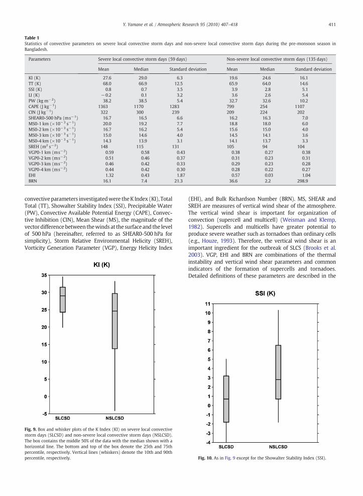
Table 1Statistics of convective parameters on severe local convective storm days and non-severe local convective storm days during the pre-monsoon season inBangladesh.

Parameters Severe local convective storm days (59 days) Non-severe local convective storm days (135 days)

Mean Median Standard deviation Mean Median Standard deviation

KI (K) 27.6 29.0 6.3 19.6 24.6 16.1TT (K) 68.0 66.9 12.5 65.9 64.0 14.6SSI (K) 0.8 0.7 3.5 3.9 2.8 5.1LI (K) −0.2 0.1 3.2 3.6 2.6 5.4PW (kg m−2) 38.2 38.5 5.4 32.7 32.6 10.2CAPE (J kg−1) 1363 1170 1283 799 254 1107CIN (J kg−1) 322 300 239 209 224 202SHEAR0-500 hPa (ms−1) 16.7 16.5 6.6 16.2 16.3 7.0MS0-1 km (×10−3 s−1) 20.0 19.2 7.7 18.8 18.0 6.0MS0-2 km (×10−3 s−1) 16.7 16.2 5.4 15.6 15.0 4.0MS0-3 km (×10−3 s−1) 15.0 14.6 4.0 14.5 14.1 3.6MS0-4 km (×10−3 s−1) 14.3 13.9 3.1 14.1 13.7 3.3SREH (m2 s−2) 148 115 131 105 94 104VGP0-1 km (ms−2) 0.59 0.58 0.43 0.38 0.27 0.38VGP0-2 km (ms−2) 0.51 0.46 0.37 0.31 0.23 0.31VGP0-3 km (ms−2) 0.46 0.42 0.33 0.29 0.23 0.28VGP0-4 km (ms−2) 0.44 0.42 0.30 0.28 0.22 0.27EHI 1.32 0.43 1.87 0.57 0.03 1.04BRN 16.1 7.4 21.3 36.6 2.2 298.9


convectiveparameters investigatedwere theK Index (KI), TotalTotal (TT), Showalter Stability Index (SSI), Precipitable Water(PW), Convective Available Potential Energy (CAPE), Convec-tive Inhibition (CIN), Mean Shear (MS), the magnitude of thevectordifference between thewinds at the surface and the levelof 500 hPa (hereinafter, referred to as SHEAR0-500 hPa forsimplicity), Storm Relative Environmental Helicity (SREH),Vorticity Generation Parameter (VGP), Energy Helicity Index

Fig. 9. Box and whisker plots of the K Index (KI) on severe local convectivestorm days (SLCSD) and non-severe local convective storm days (NSLCSD).The box contains the middle 50% of the data with the median shown with ahorizontal line. The bottom and top of the box denote the 25th and 75thpercentile, respectively. Vertical lines (whiskers) denote the 10th and 90thpercentile, respectively.

(EHI), and Bulk Richardson Number (BRN). MS, SHEAR andSREH are measures of vertical wind shear of the atmosphere.The vertical wind shear is important for organization ofconvection (supercell and multicell) (Weisman and Klemp,1982). Supercells and multicells have greater potential toproduce severe weather such as tornadoes than ordinary cells(e.g., Houze, 1993). Therefore, the vertical wind shear is animportant ingredient for the outbreak of SLCS (Brooks et al.2003). VGP, EHI and BRN are combinations of the thermalinstability and vertical wind shear parameters and commonindicators of the formation of supercells and tornadoes.Detailed definitions of these parameters are described in the

Fig. 10. As in Fig. 9 except for the Showalter Stability Index (SSI).

Fig. 11. As in Fig. 9 except for the Lifted Index (LI). Fig. 13. As in Fig. 9 except for the Convective Available Potential Energy(CAPE).


Appendix. Table 1 shows statistics on convective parameters onSLCSD and NSLCSD.

We determined the statistical significance between con-vective parameters on SLCSD and those on NSLCSD using the Ztest. The result indicates that all thermodynamic parametersand combination parameters except for the TT and the BRNhave statistical significance with the confidence level of 99%.However, all dynamic parameters have no statistical signifi-cance with the level of 99%. The SLCSD identified in this study

Fig. 12. As in Fig. 9 except for the Perceptible Water (PW). Fig. 14. As in Fig. 9 except for the Convective Inhibition (CIN).

include various severe convective weather events. If we candiscriminate between supercell and non-supercell, or tornadoand non-tornado, dynamic parameters may be able todifferentiate between these two categories. Therefore, theresult in the present studydoes not necessarily indicate that thevertical wind shear is not important for the formation oftornadoes and supercells during the pre-monsoon season inBangladesh. In this study, we focus on convective parameters

Fig. 15. As in Fig. 9 except for the Vorticity Generation Parameter betweenthe surface and 1 km AGL (VGP0-1 km).



with the statistical significance of the level of 99% betweenSLCSD and NSLCSD.

We show box and whisker plots for each convectiveparameter in Figs. 9–19. The box contains the middle 50% ofthe data with the median shown with a horizontal line. Thebottom and top of the box denote the 25th and 75th percentile,


respectively. Vertical lines (whiskers) denote the10th and 90thpercentile, respectively.

3.2.1. K IndexThe mean andmedian values for the KI on SLCSD are 27.6 K

and 29.0 K, and greater than those on NSLCSD (19.6 K and


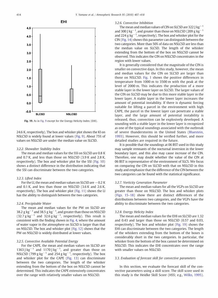
Fig. 19. As in Fig. 9 except for the Energy Helicity Index (EHI).


24.6 K, respectively). The box andwhisker plot shows the KI onNSLCSD is widely found at lower values (Fig. 9). About 75% ofvalues on NSLCSD are under the median value on SLCSD.

3.2.2. Showalter Stability IndexThemean andmedian values for the SSI on SLCSD are 0.8 K

and 0.7 K, and less than those on NSLCSD (3.9 K and 2.8 K,respectively). The box and whisker plot for the SSI (Fig. 10)shows a distinct difference in the distribution indicating thatthe SSI can discriminate between the two categories.

3.2.3. Lifted IndexFor the LI, themeanandmedianvalues on SLCSDare−0.2 K

and 0.1 K, and less than those on NSLCSD (3.6 K and 2.6 K,respectively). The box and whisker plot (Fig. 11) shows the LIhas the ability to distinguish between the two categories.

3.2.4. Precipitable WaterThe mean and median values for the PW on SLCSD are

38.2 g kg−1 and38.5 g kg−1, and greater than thoseonNSLCSD(32.7 g kg−1 and 32.6 g kg−1, respectively). This result isconsistent with the finding shown in Fig. 4, where the amountof water vapor in the atmosphere on SLCSD is larger than thaton NSLCSD. The box and whisker plot (Fig. 12) shows that thePW on NSLCSD is widely distributed at lower values.

3.2.5. Convective Available Potential EnergyFor the CAPE, the mean and median values on SLCSD are

1363 J kg−1 and 1170 J kg−1, and greater than those onNSLCSD (799 g kg−1 and 254 g kg−1, respectively). The boxand whisker plot for the CAPE (Fig. 13) can discriminatebetween the two categories. The length of the whiskerextending from the bottom of the box on NSLCSD cannot bedetermined. This indicates the CAPE extensively concentratesover the range with relatively smaller values on NSLCSD.

3.2.6. Convective InhibitionThemeanandmedianvaluesof CINonSLCSDare 322 J kg−1

and 300 J kg−1, and greater than those on NSLCSD (209 g kg−1

and 224 g kg−1, respectively). The box andwhisker plot for theCIN (Fig. 14) shows this parameter can distinguish between thetwo categories. More than 50% of data on NSLCSD are less thanthe median value on SLCSD. The length of the whiskerextending from the bottom of the box on NSLCSD cannot beobserved. This indicates the CIN on NSLCSD concentrates in theregion with lower values.

It is generally considered that the magnitude of the CIN issmaller on convective days. In this study, however, the meanand median values for the CIN on SLCSD are larger thanthose on NSLCSD. Fig. 1 shows the positive differences intemperature from 1000 m to 3500 m with the peak at thelevel of 2000 m. This indicates the production of a morestable layer in the lower layer on SLCSD. The larger values ofthe CIN on SLCSD may be due to this more stable layer in thelower layer. A stable layer in the lower layer increases theamount of potential instability. If there is dynamic forcingsuitable for lifting a parcel in the environment with highCAPE, the parcel in the lowest layer can penetrate a stablelayer, and the large amount of potential instability isreleased, thus, convection can be explosively developed. Asounding with a stable layer in the lower layer is recognizedas one of the typical soundings associated with the outbreakof severe thunderstorms in the United States (Bluestein,1993). However, this should be verified further, and moredetailed studies are required in the future.

It is possible that the soundings at 06 BST used in this studymay sample remnants of the nocturnal inversion in the lowerboundary layer, and this also may cause increase of the CIN.Therefore, one may doubt whether the value of the CIN at06 BST is representative of the environment of SLCS. We focuson comparing the CIN on SLCSD with that on NSLCSD in thisstudy and emphasize that the difference of the CINbetween thetwo categories can be found with the statistical significance.

3.2.7. Vorticity Generation ParameterThemean andmedian values for all the VGPs on SLCSD are

greater than those on NSLCSD. The box and whisker plots(Figs. 15–18) show there are distinct differences of thedistributions between two categories, and the VGPs have theability to discriminate between the two categories.

3.2.8. Energy Helicity IndexThemean andmedian values for the EHI on SLCSD are 1.32

and 0.43 and larger than those on NSLCSD (0.57 and 0.03,respectively). The box and whisker plot (Fig. 19) shows theEHI can discriminate between the two categories. The lengthof the whiskers extending from the bottom of the boxes isconsiderably short in the two categories. In particular, thewhisker from the bottom of the box cannot be determined onNSLCSD. This indicates the EHI concentrates over the rangewith smaller values on NSLCSD.

3.3. Evaluation of forecast skill for convective parameters

In this section, we evaluate the forecast skill of the con-vective parameters using a skill score. The skill score used inthis study is the Heidke Skill Score (HSS; e.g., Wilks, 1995).

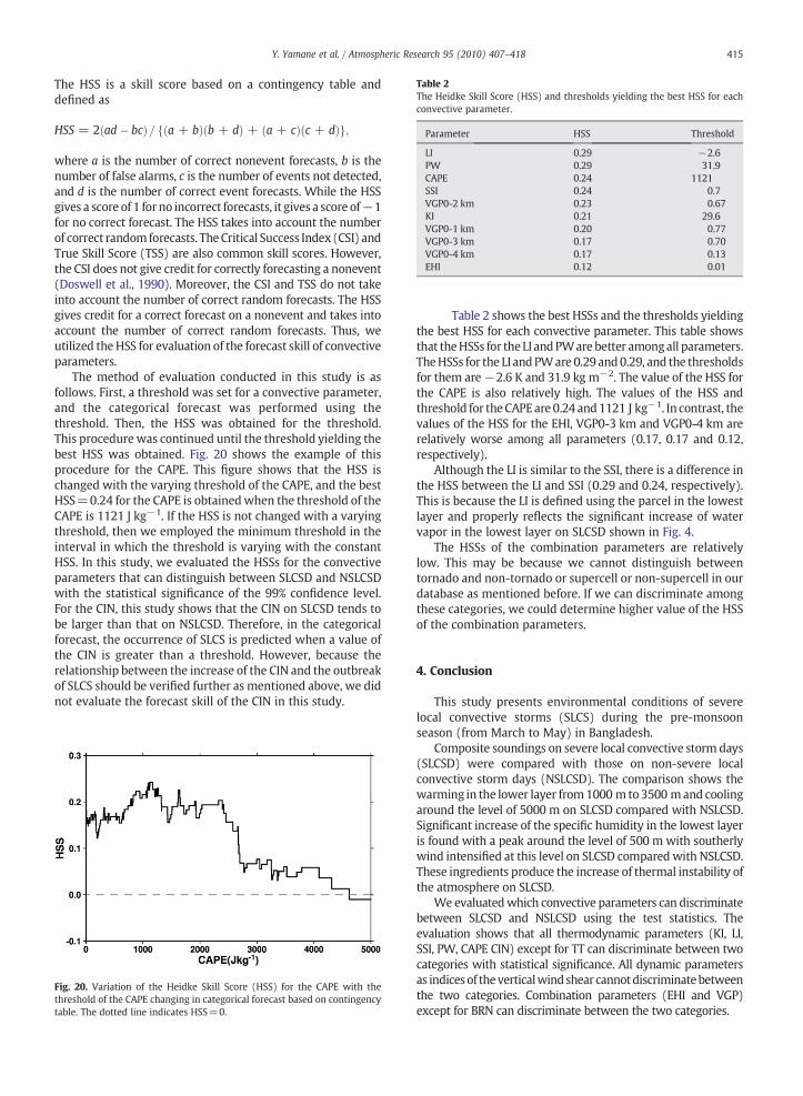
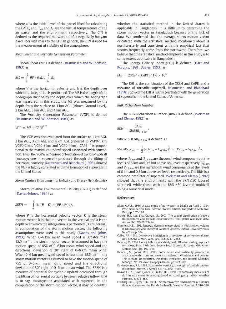
Table 2The Heidke Skill Score (HSS) and thresholds yielding the best HSS for eachconvective parameter.

Parameter HSS Threshold

LI 0.29 −2.6PW 0.29 31.9CAPE 0.24 1121SSI 0.24 0.7VGP0-2 km 0.23 0.67KI 0.21 29.6VGP0-1 km 0.20 0.77VGP0-3 km 0.17 0.70VGP0-4 km 0.17 0.13EHI 0.12 0.01


The HSS is a skill score based on a contingency table anddefined as

HSS = 2ðad� bcÞ= fða + bÞðb + dÞ + ða + cÞðc + dÞg;

where a is the number of correct nonevent forecasts, b is thenumber of false alarms, c is the number of events not detected,and d is the number of correct event forecasts. While the HSSgives a score of 1 forno incorrect forecasts, it gives a score of−1for no correct forecast. The HSS takes into account the numberof correct random forecasts. TheCritical Success Index (CSI) andTrue Skill Score (TSS) are also common skill scores. However,the CSI does not give credit for correctly forecasting a nonevent(Doswell et al., 1990). Moreover, the CSI and TSS do not takeinto account the number of correct random forecasts. The HSSgives credit for a correct forecast on a nonevent and takes intoaccount the number of correct random forecasts. Thus, weutilized the HSS for evaluation of the forecast skill of convectiveparameters.

The method of evaluation conducted in this study is asfollows. First, a threshold was set for a convective parameter,and the categorical forecast was performed using thethreshold. Then, the HSS was obtained for the threshold.This procedure was continued until the threshold yielding thebest HSS was obtained. Fig. 20 shows the example of thisprocedure for the CAPE. This figure shows that the HSS ischanged with the varying threshold of the CAPE, and the bestHSS=0.24 for the CAPE is obtainedwhen the threshold of theCAPE is 1121 J kg−1. If the HSS is not changed with a varyingthreshold, then we employed the minimum threshold in theinterval in which the threshold is varying with the constantHSS. In this study, we evaluated the HSSs for the convectiveparameters that can distinguish between SLCSD and NSLCSDwith the statistical significance of the 99% confidence level.For the CIN, this study shows that the CIN on SLCSD tends tobe larger than that on NSLCSD. Therefore, in the categoricalforecast, the occurrence of SLCS is predicted when a value ofthe CIN is greater than a threshold. However, because therelationship between the increase of the CIN and the outbreakof SLCS should be verified further as mentioned above, we didnot evaluate the forecast skill of the CIN in this study.

Fig. 20. Variation of the Heidke Skill Score (HSS) for the CAPE with thethreshold of the CAPE changing in categorical forecast based on contingencytable. The dotted line indicates HSS=0.

Table 2 shows the best HSSs and the thresholds yieldingthe best HSS for each convective parameter. This table showsthat theHSSs for the LI andPWare better amongall parameters.TheHSSs for the LI andPWare 0.29 and0.29, and the thresholdsfor them are−2.6 K and 31.9 kg m−2. The value of the HSS forthe CAPE is also relatively high. The values of the HSS andthreshold for theCAPEare 0.24 and1121 J kg−1. In contrast, thevalues of the HSS for the EHI, VGP0-3 km and VGP0-4 km arerelatively worse among all parameters (0.17, 0.17 and 0.12,respectively).

Although the LI is similar to the SSI, there is a difference inthe HSS between the LI and SSI (0.29 and 0.24, respectively).This is because the LI is defined using the parcel in the lowestlayer and properly reflects the significant increase of watervapor in the lowest layer on SLCSD shown in Fig. 4.

The HSSs of the combination parameters are relativelylow. This may be because we cannot distinguish betweentornado and non-tornado or supercell or non-supercell in ourdatabase as mentioned before. If we can discriminate amongthese categories, we could determine higher value of the HSSof the combination parameters.

4. Conclusion

This study presents environmental conditions of severelocal convective storms (SLCS) during the pre-monsoonseason (from March to May) in Bangladesh.

Composite soundings on severe local convective storm days(SLCSD) were compared with those on non-severe localconvective storm days (NSLCSD). The comparison shows thewarming in the lower layer from1000 m to3500 mand coolingaround the level of 5000 m on SLCSD compared with NSLCSD.Significant increase of the specific humidity in the lowest layeris found with a peak around the level of 500 m with southerlywind intensified at this level on SLCSD compared with NSLCSD.These ingredients produce the increase of thermal instability ofthe atmosphere on SLCSD.

We evaluatedwhich convective parameters can discriminatebetween SLCSD and NSLCSD using the test statistics. Theevaluation shows that all thermodynamic parameters (KI, LI,SSI, PW, CAPE CIN) except for TT can discriminate between twocategories with statistical significance. All dynamic parametersas indicesof theverticalwindshear cannotdiscriminatebetweenthe two categories. Combination parameters (EHI and VGP)except for BRN can discriminate between the two categories.


We evaluated the forecast skill of convective parametersusing the Heidke Skill Score (HSS). While the HSS of the LIand PW is better among all parameters, the HSS of the EHI isthe worst. In addition, we can provide the critical valuesthat are helpful in forecasting the likelihood of the occur-rence of SLCS.

The current study shows that differences with thestatistical significance between SLCSD and NSLCSD can bedetected by analysis with rawinsonde data at 06 BST inDhaka, and some convective parameters computed with therawinsonde data can discriminate between the two catego-ries. This indicates that the rawinsonde data at 06 BST inDhaka are to some extent representative of the environmentof SLCS and useful for the forecasting. Now, BMD does nothave an effective method for the forecasting of SLCS. Theresults of this study will be helpful for introducing forecast-ing using convective parameters based on the rawinsondedata at 06 BST in Dhaka. The convective parametersemployed in this study were developed in another area,especially the United States. Modification of the parametersmay be efficient for further improving the forecast skill ofconvective parameters.

Acknowledgments

We wish to thank Bangladesh Meteorological Departmet(BMD) for providing rawinsonde data at Dhaka. This studywas supported by Program for Improvement of ResearchEnvironment for Young Researchers from Special Coordina-tion Funds for Promoting Science and Technology (SCF)commissioned by the Ministry of Education, Culture, Sports,Science and Technology (MEXT) of Japan. This work was alsosupported in part by Global COE Program: “In search ofSustainable Humanosphere in Asia and Africa”, MEXT, Japan.

Appendix A

In this section, we describe details of the convectiveparameters used in this study.

K Index

The K Index (KI) is defined (George, 1960) as

KI = T850hPa � T500hPa + Td850hPa � ðT700hPa � Td700hPaÞ;

where T is temperature, and Td is dew point temperature.T850 hPa−T500 hPa indicates the lapse rate of temperaturebetween the lower layer and middle layer. Td850 hPa indicatesthe moisture content in the lower layer. T700 hPa−Td700 hPa isa measure of the reduction of negative buoyancy throughentrainment of dry air. The KI exceeding 28 K indicates thelikelihood of convection (Fuelbarg and Biggar, 1994).

Total Total

The Total Total (TT) is defined (Sadowski and Rieck, 1977)as

TT = ðT850hPa + Td850hPaÞ � 2T500hPa;

where T is the temperature, and Td is the dewpoint temperature.

Showalter Stability Index

The Showalter Stability Index (SSI) is defined (Showalter,1953) as

SSI = T500hPa � Tp500hPa;

where Tp500 hPa is the temperature of a parcel lifted adiabat-ically from 850 hPa until saturated, and then moist adiabat-ically to 500 hPa. T500 hPa is the temperature at 500 hPa.Negative SSI indicates the likelihood of convective activity.

Lifted Index

The Lifted Index (LI) is defined (Galway, 1956) as

LI = T500hPa � Tp500hPa⁎ ;

where Tp⁎500 hPa is the temperature of a parcel with the meantemperature and dewpoint temperature in the lowest 100 hPalifted adiabatically until saturated, and then moist adiabati-cally to 500 hPa. T500 hPa is the temperature at 500 hPa.Negative LI indicates the likelihood of convective activity.The LI explicitly reflects the condition in the boundary layercompared with the SSI.

Precipitable Water

Precipitable Water (PW) is defined (Huschke, 1959) as

PW = ∫0

Ps

qdp≅ ∫100hPa

Ps

qdp;

where Ps is the surface pressure, and q is the specific humidity.In this study, the top pressure is defined as 100 hPa because ofthe scarce amount of water vapor above 100 hPa.

Convective Available Potential Energy

CAPE is defined (Moncrieff and Miller, 1976) as

CAPE = g ∫zEL

zLFC

ðTvp � TvÞ=Tvdz;

where g is the gravitational acceleration, zLFC is the level ofLFC (level of free convection), and zEL is the equilibrium level,where the temperature excess of a parcel lifted from the LFCfirst becomes zero above the LFC, and, Tvp and Tv are thevirtual temperatures of the air parcel and the environment,respectively. The CAPE is defined as the net work of theenvironment on a parcel per unit mass lifted from zLFC to zELand the measurement of the development of convection. Wechose a parcel with thermodynamic properties averaged overthe lowest 50 hPa.

Convective Inhibition

Convective Inhibition (CIN) is defined (Colby, 1984) as

CIN = g ∫zLFC

zi

ðTvp � TvÞ= Tvdz;


where zi is the initial level of the parcel lifted for calculatingthe CAPE, and, Tvp and Tv are the virtual temperatures of theair parcel and the environment, respectively. The CIN isdefined as the required net work to lift a negatively buoyantparcel per unit mass to the LFC. In general, the CIN is used forthe measurement of stability of the atmosphere.

Mean Shear and Vorticity Generation Parameter

Mean Shear (MS) is defined (Rasmussen and Wilhemson,1983) as

MS = ∫h

0

∂V = ∂zdz= ∫h

0

dz;

where V is the horizontal velocity and h is the depth overwhich the integration is performed. TheMS is the length of thehodograph divided by the depth over which the hodographwas measured. In this study, the MS was measured by thedepth from the surface to 1 km AGL (Above Ground Level),2 km AGL, 3 km AGL and 4 km AGL.

The Vorticity Generation Parameter (VGP) is defined(Rasmussen and Wilhemson, 1983) as

VGP = MS × CAPE1=2

The VGP was also evaluated from the surface to 1 km AGL,2 km AGL, 3 km AGL and 4 km AGL (referred to VGP0-1 km,VGP0-2 km, VGP0-3 km and VGP0-4 km). CAPE1/2 is propor-tional to the maximum updraft speed associated with convec-tion. Thus, theVGP is ameasure of formation of cyclonic updraft(mesocyclone in supercell) produced through the tilting ofhorizontal vorticity. Rasmussen and Blanchard (1998) showedthe VGP is highly correlated with the formation of supercells inthe United States.

Storm Relative Environmental Helicity and Energy Helicity Index

Storm Relative Environmental Helicity (SREH) is defined(Davies-Johnes, 1984) as

SREH = � ∫h

0

k ⋅ðV � CÞ × ð∂V = ∂zÞdz;

where V is the horizontal velocity vector, C is the stormmotion vector, k is the unit vector in the vertical and h is thedepth over which the integration is performed (3 km herein).In computation of the storm motion vector, the followingassumptions were used in this study (Davies and Johns,1993). When 0–6 km mean wind speed is greater than15.5 ms−1, the storm motion vector is assumed to have themotion speed of 85% of 0–6 km mean wind speed and thedirectional deviation of 20° right of 0–6 km mean wind.When 0–6 km mean wind speed is less than 15.5 ms−1, thestorm motion vector is assumed to have the motion speed of75% of 0–6 km mean wind speed and the directionaldeviation of 30° right of 0–6 km mean wind. The SREH is ameasure of potential for cyclonic updraft produced throughthe tilting of horizontal vorticity by storm relative inflow, thatis to say, mesocyclone associated with supercell. In thecomputation of the storm motion vector, it may be doubtful

whether the statistical method in the United States isapplicable in Bangladesh. It is difficult to determine thestorm motion vector in Bangladesh because of the lack ofdata. We confirmed that the average storm motion vectorcalculated with the statistical method mentioned above isnorthwesterly and consistent with the empirical fact thatstorms frequently come from the northwest. Therefore, webelieve that the statistical method employed in this study is tosome extent applicable in Bangladesh.

The Energy Helicity Index (EHI) is defined (Hart andKorotky, 1991; Davies, 1993) as

EHI = ðSREH × CAPEÞ= 1:6 × 105

The EHI is the combination of the SREH and CAPE, and ameasure of tornadic supercell. Rasmussen and Blanchard(1998) showed the EHI is highly correlatedwith the generationof supercells in the United States of America.

Bulk Richardson Number

The Bulk Richardson Number (BRN) is defined (Weismanand Klemp, 1982) as

BRN =CAPE

SHEAR0�6 km;

where SHEAR0–6 km is defined as

SHEAR0�6 km =12fðU6 km � U0:5 kmÞ2 + ðV6 km � V0:5 kmÞ2g;

whereU6 km andU0.5 km are the zonalwind components at thelevels of 6 km and 0.5 km above sea level, respectively. V6 km

and V0.5 km are the meridional wind components at the levelsof 6 km and 0.5 km above sea level, respectively. The BRN is acommon predictor of supercell. Weisman and Klemp (1982)showed that the environments with the BRN≤50 favoredsupercell, while those with the BRN≥50 favored multicellusing a numerical model.

References

Alam, Q.M.S., 1986. A case study of nor'wester in Dhaka on April 7 1984.Proc. Seminar on Local Severe Storms, Dhaka, Bangladesh Meteorol.Dep, pp. 167–180.

Brooks, H.E., Lee, J.W., Craven, J.P., 2003. The spatial distribution of severethunderstorm and tornado environments from global reanalysis data.Atmos. Res. 67–68, 73–94.

Bluestein, H.B., 1993. Synoptic–dynamic meteorology in midlatitudes: volumeII. Observations and Theory of Weather Systems. Oxford University Press,New York, p. 594.

Colby, F.P., 1984. Convective inhibition as a predictor of convection duringAVE-SESAM-2. Mon. Wea. Rev. 112, 2239–2252.

Davies, J.M., 1993. Hourly helicity, instability, and EHI in forecasting supercelltornadoes. Proc. 17th Conf. Severe Local Storms, St. Louis, MO: Amer.Meteor. Soc. , pp. 107–111.

Davies, J.M., Johns, R.H., 1993. Some wind and instability parametersassociated with strong and violent tornadoes. 1. Wind shear and helicity,The Tornado: Its Structure, Dynamics, Prediction, and Hazard. Geophys.Monogr., No. 79: Ame. Geophys. Union, pp. 573–582.

Davies-Johnes, R.P., 1984. Streamwise vorticity: the origin of updraft rotationin supercell storms. J. Atmos. Sci. 41, 2991–3006.

Doswell, C.A., Davies-Jones, R., Keller, D.L., 1990. On summary measures ofskill in rare event forecasting based on contingency tables. WeatherForecast. 5, 576–585.

Fuelbarg, H.E., Biggar, D.G., 1994. The preconvective environment of summerthunderstorms over the Florida Panhandle. Weather Forecast. 9, 316–326.


Galway, J.G., 1956. The lifted index as a predictor of latent instability. Bull.Amer. Meteor. Soc. 37, 528–529.

George, J.J., 1960. Weather Forecasting for Aeronautics. Academic Press,p. 637.

Hart, J.A., Korotky, W., 1991. The SHARP workstation v1.50 users guide.National Weather Service, NOAA: US. Dept. of Commerce, p. 30.

Houze, R.A., 1993. Cloud Dynamics. Elsevier, New York, p. 570.Huschke, R.E., 1959. Glossary of Meteorology. Amer. Meteor. Soc. 638.Karmakar, S., Alam,M.M., 2006. Instability of the troposphere associated with

thunderstorms/nor'westers over Bangladesh during the pre-monsoonseason. MAUSAM 57 (4), 629–638.

Maddox, R.A., 1976. An evaluation of tornado proximity wind and stabilitydata. Mon. Weather Rev. 104, 133–142.

Mowla, K.G., 1986. A scientific note on the nor'wester of 14th April 1969 inBangladesh. Proc. Seminar on Local Severe Storms, Dhaka, BangladeshMeteorol. Dep, pp. 10–33.

Moncrieff, M., Miller, M.J., 1976. The dynamics and simulation of tropicalcumulonimbus and squall lines. Quart. J. Roy. Meteor. Soc. 102, 373–394.

Rasmussen, E.N.,Wilhemson, R.B., 1983. Relationships between storm character-istics and 1200 GMT hodographs, low-level shear, and stability. Proc. 13thConf. on Severe Local Storms, Tulsa, OK: Amer. Meteor. Soc., pp. J5–J8.

Rasmussen, E.N., Blanchard, D.O., 1998. A baseline climatology of sounding-derived supercell and tornado forecast parameters. Weather Forecast.13, 1148–1164.

Sadowski, A.F., Rieck, R.E., 1977. Technical Procedures Bulletin No. 207:Stability indices. National Weather Service, Silver Spring, MD, p. 8.

Showalter, A.K., 1953. A stability index of thunderstorm forecasting. Bull.Amer. Meteor. Soc. 34, 250–252.

Yamane, Y., Hayashi, T., Dewan, A.M., Akter, F., 2009. Severe local convectivestorms in Bangladesh: Part I. Climatology. Atmos. Res. doi:10.1016/j.atmosres2009.11.004.

Weisman, M.L., Klemp, J.B., 1982. The dependence of numerically simulatedconvective storms on vertical wind shear and buoyancy. Mon. WeatherRev. 110, 504–520.

Wilks, D.S., 1995. Statistical Methods in the Atmospheric Sciences. AcademicPress, New York. 467 pp.

Documents

Severe local convective storms in Bangladesh: Part II