Setting up an SPSS data file - SAGE Publications · Setting up an SPSS data file This chapter will introduce SPSS, ... statistics package (other than common spreadsheet programs such

2Setting up an SPSS data file

This chapter will introduce SPSS, which is a widely used statistical package for analyzingdata.

Obtaining a copy of SPSS

To conduct the procedures detailed in this book for yourself, using the data files on the CD,you need a copy of SPSS. At the time of printing the latest version of SPSS was Version 13,but this book is relevant for all versions from 10 and after. SPSS is sold as a Base system foran annual license fee plus annual renewal charge, plus add-on modules that require additionalcost and extend the functionality of the Base. This text will cover the functions that areavailable as part of the Base so that it is relevant to all users of this program, regardless of theconfiguration. Those who do have add-on modules should explore these, however, to see ifthey provide alternative and better options for obtaining the statistical results we describe inthe rest of the book. There are several options to obtain a copy of SPSS Base:

1. Purchase a commercial version of SPSS. This can be done through a software retailer oron-line (www.spss.com). The initial annual fee is substantial, although the annual upgradeis much cheaper. A demonstration copy can be downloaded for free from the SPSSwebsite, but this has a limited period of use.

2. Access a site license copy. If you belong to a large organization such as a university orpublic sector department, your organization may have negotiated a site license with SPSSfor installation and use of the program. You should check with the relevant people whomanage software licenses to see if you can obtain a copy of the program through such anarrangement and what the licensing conditions include.

3. Purchase an SPSS Graduate Pack. If you are a university or college student you may beable to purchase a Graduate Pack from your campus bookstore, which includes a manualand copy of the software at a much lower price than the commercial version. As with anysoftware you purchase, however, you should check the licensing details before purchase.

4. Purchase a Student Version. A Student Version of the program is available at a relativelyinexpensive price. This does not have the full functionality of the commercial version orGraduate Pack; it is limited to 1500 cases and 50 variables. However, it is suitable for mostof the needs of an introductory user for non-commercial purposes. Prentice-Hall distributesSPSS Student Version through university and college bookstores around the world. Simplypresent your valid student identification. If your campus bookstore does not carry SPSSStudent Version, order the software on-line at www.prenhall.com, or ask the bookstoremanager to contact the local Prentice-Hall distribution office.

Alternatives to SPSS

This text details SPSS procedures for statistical analysis because it is the most widely usedstatistics package (other than common spreadsheet programs such as Excel, which can beused for complex statistical analysis but are really designed for other purposes). This text does

18 Statistics for Research

not use SPSS because it is the best; readers will note my frustration with this program and itspeculiarities as they read the following chapters. It is only appropriate therefore to draw yourattention to alternatives that are available and which you may choose rather than SPSS. Toassist this the CD accompanying this book contains all the data files for the followingexamples in tab-delimited ASCII format so that they can be imported into a wide range ofalternative software. There are three broad classes of alternatives to SPSS.

1. Other comprehensive commercial programs. There are many commercial alternatives toSPSS such as GB-Stat, InStat, JMP, Minitab, SAS, and StatA. A full list of such packagesis available at www.statistics.com/content/commsoft/fulllist.php3

2. Free comprehensive programs. An exciting development in recent years is the amount offree software that are available, usually produced under the open source license, and thisincludes some useful statistical analysis software. A listing of such software is available atfreestatistics.altervista.org/stat.php and members.aol.com/johnp71/javasta2.html Of these,three are particularly worth mentioning. Epi Info has been developed by the US Center forDisease Control (www.cdc.gov/epiinfo) mainly for the use of epidemiologists and otherhealth scientists, although researchers from other disciplines will find this program suitableto their needs. An open source version of Epi Info, called OpenEpi, which runs on allplatforms and in a web browser, is available from www.openepi.com Second, the programStatCrunch (www.statcrunch.com) allows users to load, analyze, and save results usingnothing more than a standard web browser, but with much of the functionality (andsometimes more) of SPSS. Last, an extremely powerful and comprehensive open sourceprogram called R is available for all platforms for free (www.r-project.org). At present itrequires some knowledge of the R programming language, but graphical user interfaces arebeing developed so that users can select commands from a drop-down menu; a phase ofdevelopment similar to that which SPSS experienced in the early 1990s.

3. Calculation pages for specific statistical pages. These are web pages that provide tools forconducting specific analysis, including many that we will cover in later chapters. We willrefer to some of these below, but a general listing of these pages is available at the webpage members.aol.com/johnp71/javastat.html or StatPages.net.

Options for data entry in SPSS

In setting up an SPSS file to undertake statistical analysis we encounter in a very practicalway many of the conceptual issues introduced in Chapter 1. Assume that in order to answerthe research questions I posed at the start of Chapter 1 I survey 200 of my statistics students.In this hypothetical survey I am interested in three separate variables: age, sex, and healthlevel. Sex is measured by classifying cases into male or female (nominal). The surveyrespondents also rate their respective health level as ‘Very healthy’, ‘Healthy’, or ‘Unhealthy’(ordinal, but with a ‘Don’t know’ option). Finally, I ask students their respective age in wholeyears on their last birthday (interval/ratio). This chapter will detail how we can record thisinformation directly in SPSS so that we can use it as an example when we learn thetechniques for statistical analysis in later chapters. However, there are other means by whichdata can be imported into SPSS other than by entering it directly, as we will do here.

1. Importing data from database, spreadsheet, or statistics programs. SPSS recognizes filescreated by other popular data programs such as Excel, Systat, Lotus, dBase, and SYLK.The range of programs and file extensions that SPSS recognizes are listed under theFile/Open/Data command; click on the File of Type: (Windows) or Enable (Macintosh)

Setting up an SPSS data file 19

option when the Open File box appears to see the full list. This is a convenient option forlarge-scale data entry, since such programs are widely available and well-known. Thusonly one copy of SPSS needs to be purchased and located on the computer where theanalysis will be conducted, with data entry performed on these other programs and thenimported into the copy of SPSS. The limitation is that data have to be entered into theseother programs in a specific way so that problems and errors are not encountered whenimporting into SPSS. These problems can sometimes be avoided by simply copying theblock of data from the other program and then pasting the data into the SPSS Data Editorand defining the variables within SPSS using the procedures we detail below.

2. Importing text files (*.txt). If you are not sure whether SPSS will read the ‘native’ versionof the data file you create in another program, you may be able to save the file as a tab-delimited text (ASCII) file. SPSS will import such a file through the File/Read Text Datacommand. An Import Wizard will then appear to assist you to bring the data across.

3. Importing from data entry programs. There are many programs available that require nospecial knowledge of SPSS (or any other data program) to facilitate data entry. Theseprograms have many advantages: for example, they often restrict the numbers that can beentered to only those that are considered valid, thus avoiding errors. They also save thedata set directly in SPSS format, or else in ASCII format that can be imported into SPSS.SPSS Inc has its own product called SPSS Data Entry, but other commercial services existsuch as Quest (www.dipolar.com). Similarly, some of the free programs listed above, suchas Epi Info also provide data entry facilities, as do on-line survey programs such asPHPSurveyor (phpsurveyor.sourceforge.net).

The SPSS Data Editor

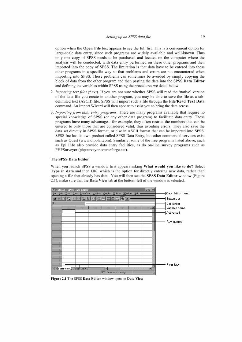
When you launch SPSS a window first appears asking What would you like to do? SelectType in data and then OK, which is the option for directly entering new data, rather thanopening a file that already has data. You will then see the SPSS Data Editor window (Figure2.1); make sure that the Data View tab at the bottom-left of the window is selected.

Figure 2.1 The SPSS Data Editor window open on Data View


Note the Data Editor menu at the top of the window. We define and analyze data byselecting commands from this menu. Usually selecting commands from the menu will bringup on the screen a small rectangular area called a dialog box, from which more specializedoptions are available, depending on the procedure we want to undertake. By the end of thisand later chapters this way of hunting through the Data Editor menu for the appropriatecommands will be very familiar. In fact, it is very similar to many other software applicationsthat readers have encountered, such as word processing and spreadsheet software.

In Figure 2.1, below the Data Editor menu bar is a Button bar that provides an alternativemeans for activating many of the commands contained within the menu. Generally we willconcentrate on using the Data Editor menu to activate SPSS commands, even thoughsometimes clicking on the relevant button on the Button bar may be quicker. We willconcentrate just on the use of menu options simply to ensure that we learn one methodconsistently; after some level of proficiency readers can then decide whether selectingcommands through the menu or by clicking on the buttons is preferable.

You should also observe that the unshaded cell at the top left of the page in Figure 2.1 has aheavy border, indicating it is the active cell. The active cell is the cell in which anyinformation will be entered if I start typing and then hit the enter-key on the keyboard. Anycell can be made active simply by pointing the cursor at it and clicking the mouse. You willthen notice a heavy border around the cell on which you have just clicked, indicating that it isthe active cell.

The Data Editor window consists of two pages, indicated by the page tabs at the bottom-leftof the Editor window. The first is the Data View page on which we enter the data for eachvariable. The Data View is the ‘data page’ on which all the information will be entered.Think of it as a blank table without any information typed into it. The Data View page ismade up of a series of columns and rows, which form little rectangles called cells. Eachcolumn will contain the information for each one of the variables, and each row will containthe information for each case. The first row of cells at the top of the columns is shaded andcontains a faint var. This row of shaded cells will contain the names of the variables whoseinformation is stored in each column. Similarly, the first column is shaded and contains faintrow numbers 1, 2, 3, etc.

The second page is the Variable View page on which we define the variables to beanalyzed. A column in the Data View page stores data for a single variable, whereas each rowin the Variable View contains the definition for a single variable.

We can switch from the Data View page to the Variable View page in one of two ways:

1. click on the Variable View tab at the bottom of the window, or

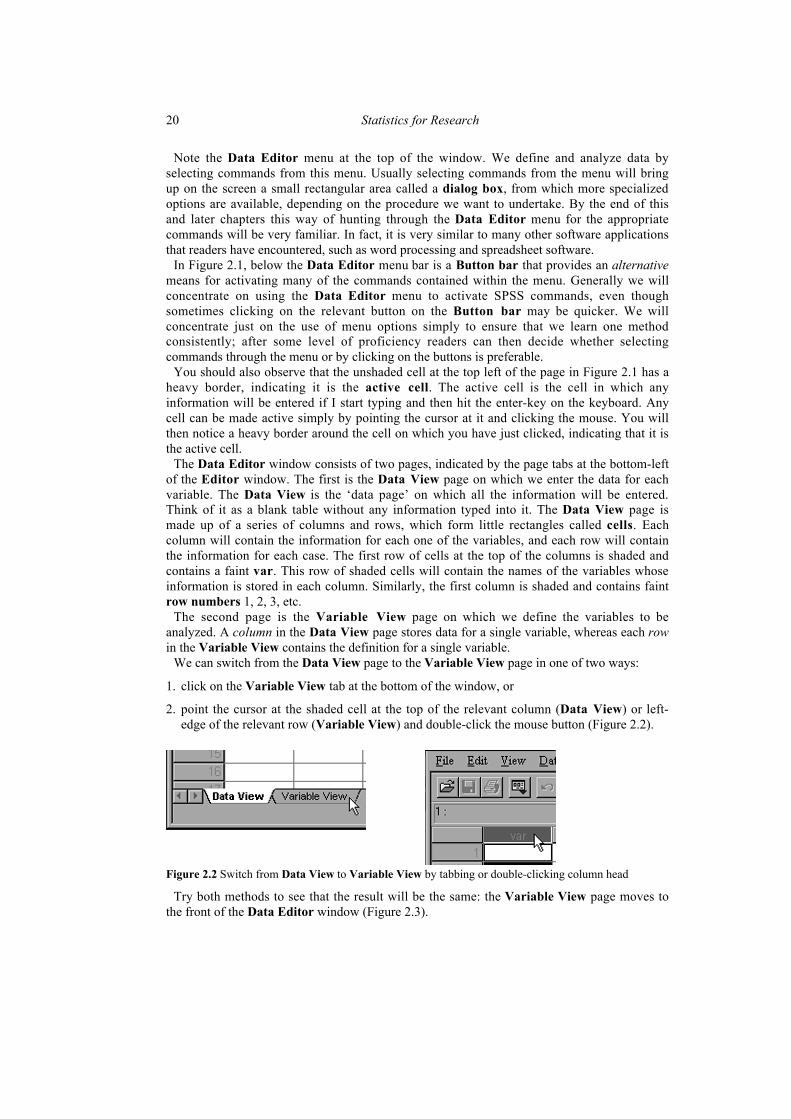
2. point the cursor at the shaded cell at the top of the relevant column (Data View) or left-edge of the relevant row (Variable View) and double-click the mouse button (Figure 2.2).

Figure 2.2 Switch from Data View to Variable View by tabbing or double-clicking column head

Try both methods to see that the result will be the same: the Variable View page moves tothe front of the Data Editor window (Figure 2.3).


Figure 2.3 The Variable View page

Each row in this page defines a single variable. We will illustrate the process of defining avariable in the Variable View page using students’ sex.

Assigning a variable name

The first task is to give the variable a name. If we make the cell below Name in the first rowactive by clicking on it, we can type in a variable name, which in this instance is sex.

There are some limitations imposed by SPSS on the names we can assign to our variables:

• In SPSS version 12 or later, a variable name can have a maximum of 64 characters madeup of letters and/or numbers. In earlier versions, only eight characters are permitted.• A variable name must begin with a letter.• A variable name cannot end with a period.• A variable name cannot contain blanks or special characters such as &, ?, !, ‘, *, or ,• A variable name must be unique. No other variable in a data file can have the same name.• A variable name appears in lower-case letters, regardless of the case in which it is typed.

Given these specific limitations, there are two schemes for naming variables in SPSS. Onescheme uses sequential names indicating where on the research instrument (thequestionnaire, interview schedule, record sheet, etc.) the variable appears. An example of thismight be to name variables q1, q2, q3a, q3b, and so on, to indicate which question number ona questionnaire generated the data for a given variable. This provides a quick and easy way ofassigning variable names and allows you to link a name directly to the research instrument onwhich the data are recorded. Its disadvantage is that the individual variable names do not givean impression of the contents of the variable.

The other variable naming scheme that is commonly adopted, and which we are using here,is descriptive names. This is a more time-consuming method, but the individual variablename, such as sex, gives a direct impression as to what the data in a given column are about.


It is also possible to use a combination of these two naming schemes. For example, wemight use sequential names for the bulk of responses to a questionnaire, but also usedescriptive names for key demographic variables such as sex and age.

Setting the data type

You should notice that as soon as you enter the variable name and strike the return key,information is also automatically entered in the subsequent cells in the first row. These aretermed default settings; things about the variable’s definition that are pre-set unless wechoose to change them.

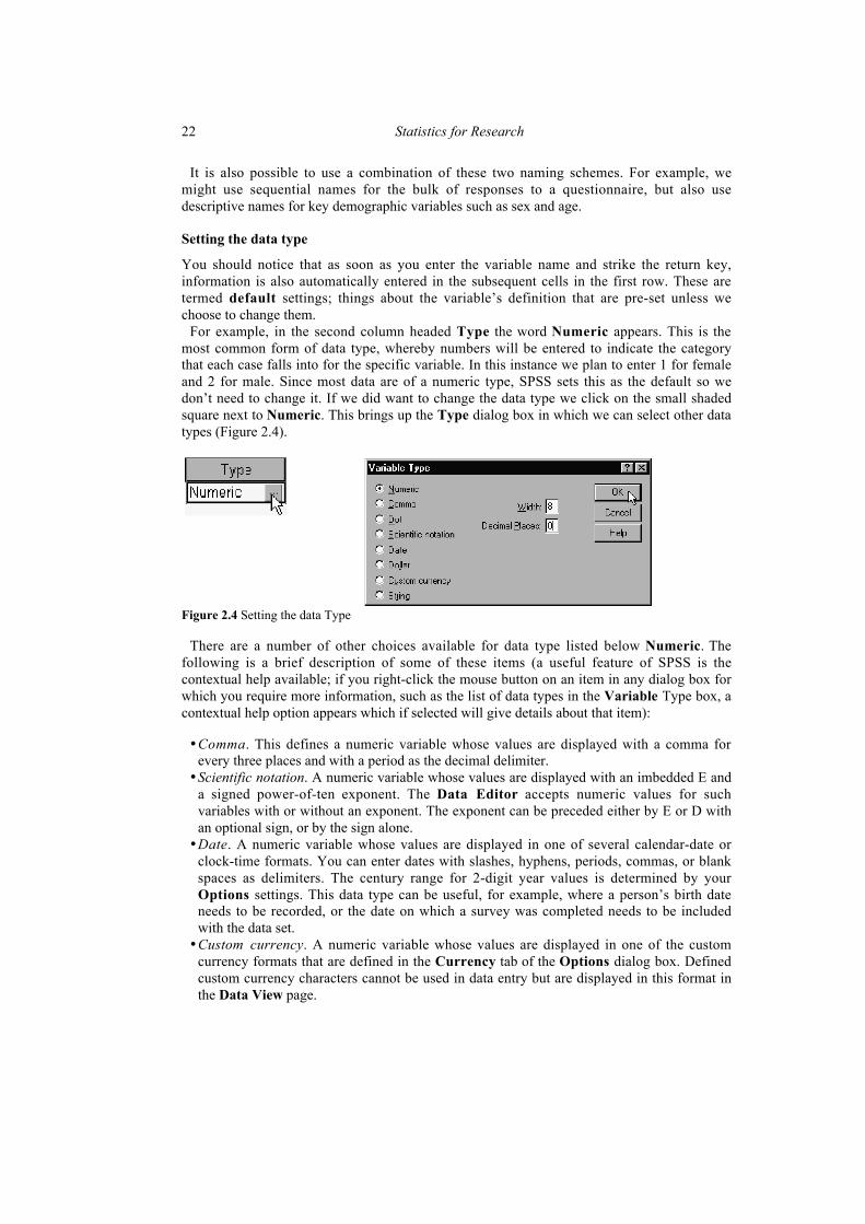
For example, in the second column headed Type the word Numeric appears. This is themost common form of data type, whereby numbers will be entered to indicate the categorythat each case falls into for the specific variable. In this instance we plan to enter 1 for femaleand 2 for male. Since most data are of a numeric type, SPSS sets this as the default so wedon’t need to change it. If we did want to change the data type we click on the small shadedsquare next to Numeric. This brings up the Type dialog box in which we can select other datatypes (Figure 2.4).

Figure 2.4 Setting the data Type

There are a number of other choices available for data type listed below Numeric. Thefollowing is a brief description of some of these items (a useful feature of SPSS is thecontextual help available; if you right-click the mouse button on an item in any dialog box forwhich you require more information, such as the list of data types in the Variable Type box, acontextual help option appears which if selected will give details about that item):

• Comma. This defines a numeric variable whose values are displayed with a comma forevery three places and with a period as the decimal delimiter.• Scientific notation. A numeric variable whose values are displayed with an imbedded E and

a signed power-of-ten exponent. The Data Editor accepts numeric values for suchvariables with or without an exponent. The exponent can be preceded either by E or D withan optional sign, or by the sign alone.• Date. A numeric variable whose values are displayed in one of several calendar-date or

clock-time formats. You can enter dates with slashes, hyphens, periods, commas, or blankspaces as delimiters. The century range for 2-digit year values is determined by yourOptions settings. This data type can be useful, for example, where a person’s birth dateneeds to be recorded, or the date on which a survey was completed needs to be includedwith the data set.• Custom currency. A numeric variable whose values are displayed in one of the custom

currency formats that are defined in the Currency tab of the Options dialog box. Definedcustom currency characters cannot be used in data entry but are displayed in this format inthe Data View page.


• String. Values of a string variable are not numeric, and hence not used in calculations.They can contain any characters up to the defined length. Upper and lower case letters areconsidered distinct. Also known as alphanumeric variable. An example is ‘m’ and ‘f’ formale and female respectively. This data type is often used for typing responses to open-ended questions that may be different for each case, and therefore cannot be precoded.

Setting the data width and decimal places

The Width of the data is the maximum number of characters that can be entered as a datumfor each case. The default setting is eight, so if we had values for a variable with more thaneight digits we would need to change this. For example, if we were entering the populationsof various countries, we would not be able to include data for countries such as the USA orChina, which have populations greater than 99,999,999. We would need to change the defaultdata Width from 8 to a higher number such as 10.

The number of Decimal Places is a ‘cosmetic’ function, in that it alters the way data aredisplayed once they are entered but does not affect what we can do. If we do not change thedefault setting of 2 decimal places, 1 will show up as 1.00 on the Data View page.

There are two ways by which the data Width and Decimal Place settings can be changedfrom the default settings.

1. In the Variable Type dialog box that we brought up to enter the data Type we also havethe option to change the variable width and the number of decimal places.

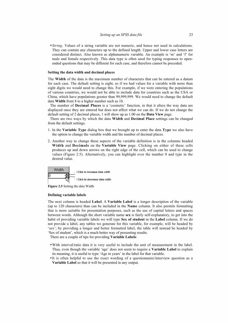
2. Another way to change these aspects of the variable definition is in the columns headedWidth and Decimals on the Variable View page. Clicking on either of these cellsproduces up and down arrows on the right edge of the cell, which can be used to changevalues (Figure 2.5). Alternatively, you can highlight over the number 8 and type in thedesired value.

Figure 2.5 Setting the data Width

Defining variable labels

The next column is headed Label. A Variable Label is a longer description of the variable(up to 120 characters) than can be included in the Name column. It also permits formattingthat is more suitable for presentation purposes, such as the use of capital letters and spacesbetween words. Although the short variable name sex is fairly self-explanatory, to get into thehabit of providing variable labels we will type Sex of student in the Label column. If we donot provide a label, any tables we generate for this variable, for example, will be headed by‘sex’; by providing a longer and better formatted label, the table will instead be headed by‘Sex of student’, which is a much better way of presenting results.

There are a couple of tips for providing Variable Labels:

• With interval/ratio data it is very useful to include the unit of measurement in the label.Thus, even though the variable ‘age’ does not seem to require a Variable Label to explainits meaning, it is useful to type ‘Age in years’ in the label for that variable.• It is often helpful to use the exact wording of a questionnaire/interview question as a

Variable Label so that it will be presented in any output.


Defining value labels

The Value Labels function allows us to specify our coding scheme; the way in whichresponses will be transformed into ‘shorthand’ codes (numbers) that allow us to performstatistical analysis, and especially to make data entry quicker. In SPSS the numerical codesare called values and the actual responses are called value labels. Thus sex has two valuelabels: female and male, and we link each label to a specific code number or value:

1 = female2 = male

Instead of typing in male or female as our data, we type in the codes assigned to these labelswhich is a much faster procedure.

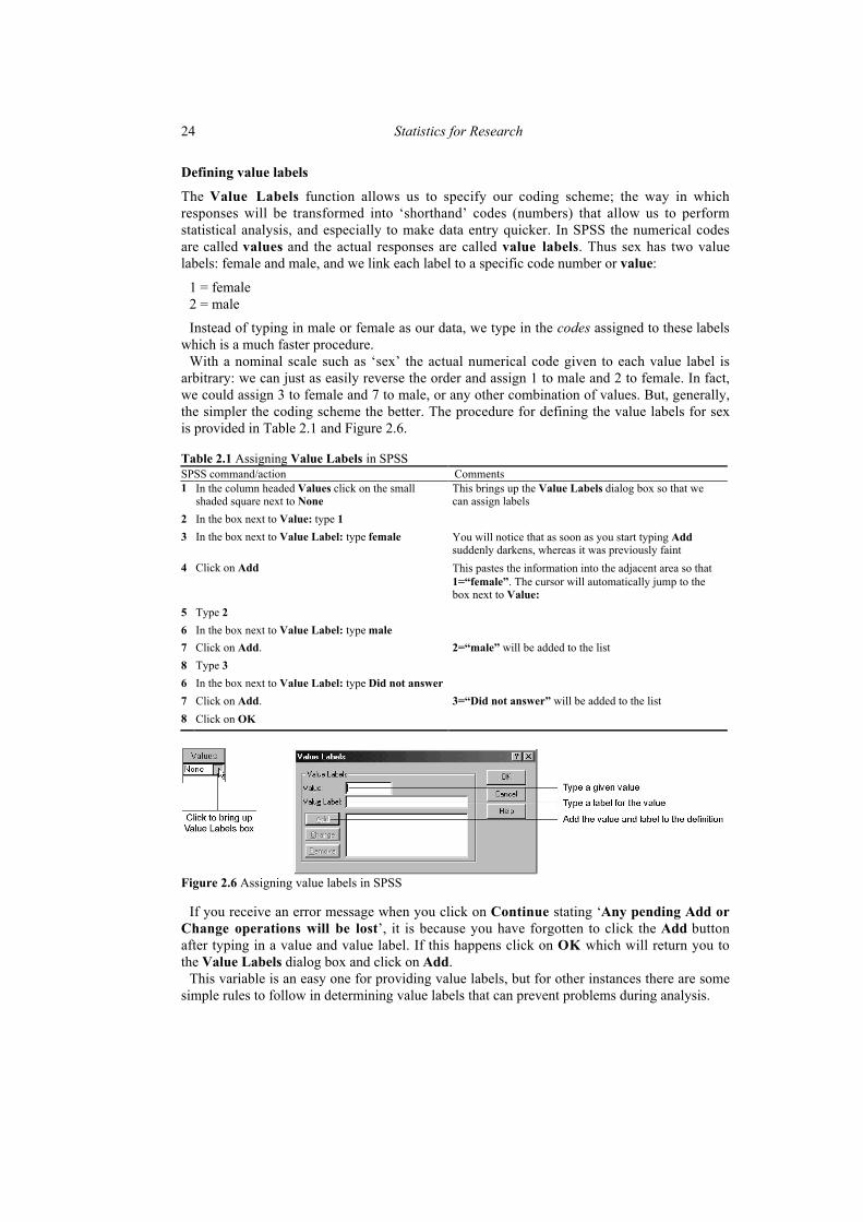
With a nominal scale such as ‘sex’ the actual numerical code given to each value label isarbitrary: we can just as easily reverse the order and assign 1 to male and 2 to female. In fact,we could assign 3 to female and 7 to male, or any other combination of values. But, generally,the simpler the coding scheme the better. The procedure for defining the value labels for sexis provided in Table 2.1 and Figure 2.6.

Table 2.1 Assigning Value Labels in SPSSSPSS command/action Comments1 In the column headed Values click on the small

shaded square next to NoneThis brings up the Value Labels dialog box so that wecan assign labels

2 In the box next to Value: type 1

3 In the box next to Value Label: type female You will notice that as soon as you start typing Addsuddenly darkens, whereas it was previously faint

4 Click on Add This pastes the information into the adjacent area so that1=“female”. The cursor will automatically jump to thebox next to Value:

5 Type 2

6 In the box next to Value Label: type male

7 Click on Add. 2=“male” will be added to the list

8 Type 3

6 In the box next to Value Label: type Did not answer

7 Click on Add. 3=“Did not answer” will be added to the list

8 Click on OK

Figure 2.6 Assigning value labels in SPSS

If you receive an error message when you click on Continue stating ‘Any pending Add orChange operations will be lost’, it is because you have forgotten to click the Add buttonafter typing in a value and value label. If this happens click on OK which will return you tothe Value Labels dialog box and click on Add.

This variable is an easy one for providing value labels, but for other instances there are somesimple rules to follow in determining value labels that can prevent problems during analysis.


1. Give separate codes for all possible types of ‘non-valid’ responses. In my hypotheticalsurvey of students, I asked students to rate their own health. The scale had three options,plus a ‘Don’t know’ option at the end of the scale for students who did not feel competentto answer. For this variable I would like to separate students that answered ‘Don’t know’and exclude them from analysis. In other words, I am treating ‘Don’t know’ as a non-validresponse. Some students, however, may simply not answer this question, and such casesalso represent non-valid responses. In other words, there are at least two reasons why astudent may not give ‘Unhealthy’, ‘Healthy’, or ‘Very healthy’ as the response; either theyresponded ‘Don’t know’ or they simply did not answer. In order to allow us to laterdistinguish between these types of non-valid responses, they are each assigned a uniquecode as follows:

1 = Unhealthy2 = Healthy3 = Very healthy4 = Don’t know5 = Did not answer

2. Give ‘null’ values a code of zero. We often encounter survey questions that have a No/Yesresponse set. In such instances we would code ‘0 = No’. The value of 0 is assigned to Nofor a deliberate reason; it is a type of response that indicates a null response: a case whereno quantity of the variable is present. Other examples of null responses are responses of‘Never’ and ‘Not at all’. Giving these responses a value of zero is very useful in lateranalysis, such as scale construction where values for a set of variables are added together.

3. For ordinal variables, make sure that the numeric scale reflects the measurement scale.Variables measured at the ordinal level have categories that indicate the relative strength inwhich the variable is present. Our scale for measuring the health of students is an example.We can say that a student who answers ‘Very healthy’ possesses more of the variable‘health’ than does a person who responds ‘Unhealthy’. This quantitative increase should bereflected in the numerical codes assigned to the categories: ‘Very healthy’ should get thebiggest number, and ‘Unhealthy’ the smallest. Our coding scheme might therefore be:

1 = Unhealthy2 = Healthy3 = Very healthy

This is particularly helpful in later data analysis, where correlations might be calculatedwith this variable.

4. Do not give interval/ratio scales complete value labels. With interval/ratio scales we do notneed to code the responses since the values ‘speak for themselves’, especially if we haveincluded the units of analysis in the Variable Label. Thus we don’t need to indicate thatcase number ‘1 = 1’, Case number ‘2 = 2’, and so on. Nor do we have to state for age that‘20 = 20 years of age’, ‘21 = 21 years of age’, and so on. The only situation in which wemight use the Value Labels function for interval/ratio data is where there are specificcategories of missing data that we want to identify (as is the cases with the age variable inour example of student survey responses).

Setting missing values

The next option in defining a variable is the Missing values option. A missing value is anumber that indicates to SPSS that the response is not valid (as we discussed in the previoussection) and should not be included in the analysis. Missing values can arise for many


reasons. For any survey question there is always the possibility that someone simply did notanswer the question, or else wrote with illegible handwriting. In another instance, a surveyquestion, such as the Health rating question in our student survey, may allow for ‘Don’tknow’ at the end of the scale and as such should not be used in analysis. A third type ofmissing data occurs where we have skip or filter questions that result in some questions beingnot applicable to all respondents. For whatever reason, when we do not have a useful datumfor an individual case for a specific variable we need to enter a missing value into the relevantcell, indicating that a valid response was not provided in that instance and therefore shouldnot be included in any analysis of that variable.

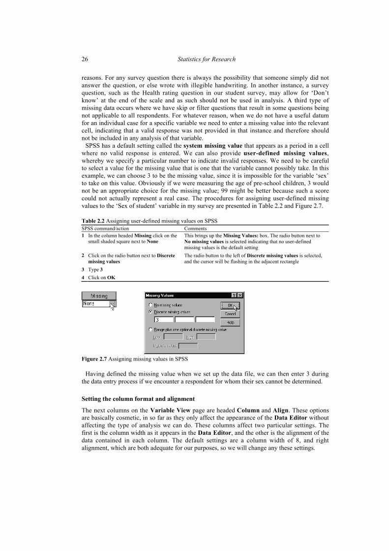
SPSS has a default setting called the system missing value that appears as a period in a cellwhere no valid response is entered. We can also provide user-defined missing values,whereby we specify a particular number to indicate invalid responses. We need to be carefulto select a value for the missing value that is one that the variable cannot possibly take. In thisexample, we can choose 3 to be the missing value, since it is impossible for the variable ‘sex’to take on this value. Obviously if we were measuring the age of pre-school children, 3 wouldnot be an appropriate choice for the missing value; 99 might be better because such a scorecould not actually represent a real case. The procedures for assigning user-defined missingvalues to the ‘Sex of student’ variable in my survey are presented in Table 2.2 and Figure 2.7.

Table 2.2 Assigning user-defined missing values on SPSSSPSS command/action Comments1 In the column headed Missing click on the

small shaded square next to NoneThis brings up the Missing Values: box. The radio button next toNo missing values is selected indicating that no user-definedmissing values is the default setting

2 Click on the radio button next to Discretemissing values

The radio button to the left of Discrete missing values is selected,and the cursor will be flashing in the adjacent rectangle

3 Type 3

4 Click on OK

Figure 2.7 Assigning missing values in SPSS

Having defined the missing value when we set up the data file, we can then enter 3 duringthe data entry process if we encounter a respondent for whom their sex cannot be determined.

Setting the column format and alignment

The next columns on the Variable View page are headed Column and Align. These optionsare basically cosmetic, in so far as they only affect the appearance of the Data Editor withoutaffecting the type of analysis we can do. These columns affect two particular settings. Thefirst is the column width as it appears in the Data Editor, and the other is the alignment of thedata contained in each column. The default settings are a column width of 8, and rightalignment, which are both adequate for our purposes, so we will change any these settings.


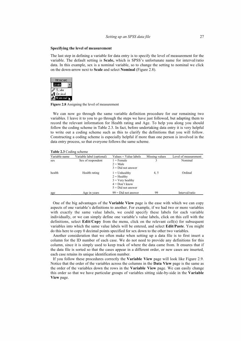
Specifying the level of measurement

The last step in defining a variable for data entry is to specify the level of measurement for thevariable. The default setting is Scale, which is SPSS’s unfortunate name for interval/ratiodata. In this example, sex is a nominal variable, so to change the setting to nominal we clickon the down-arrow next to Scale and select Nominal (Figure 2.8).

Figure 2.8 Assigning the level of measurement

We can now go through the same variable definition procedure for our remaining twovariables. I leave it to you to go through the steps we have just followed, but adapting them torecord the relevant information for Health rating and Age. To help you along you shouldfollow the coding scheme in Table 2.3. In fact, before undertaking data entry it is very helpfulto write out a coding scheme such as this to clarify the definitions that you will follow.Constructing a coding scheme is especially helpful if more than one person is involved in thedata entry process, so that everyone follows the same scheme.

Table 2.3 Coding schemeVariable name Variable label (optional) Values = Value labels Missing values Level of measurementsex Sex of respondent 1 = Female

2 = Male3 = Did not answer

3 Nominal

health Health rating 1 = Unhealthy2 = Healthy3 = Very healthy4 = Don’t know5 = Did not answer

4, 5 Ordinal

age Age in years 99 = Did not answer 99 Interval/ratio

One of the big advantages of the Variable View page is the ease with which we can copyaspects of one variable’s definitions to another. For example, if we had two or more variableswith exactly the same value labels, we could specify these labels for each variableindividually, or we can simply define one variable’s value labels, click on this cell with thedefinitions, select Edit/Copy from the menu, click on the relevant cell(s) for subsequentvariables into which the same value labels will be entered, and select Edit/Paste. You mightdo this here to copy 0 decimal points specified for sex down to the other two variables.

Another consideration that we often make when setting up a data file is to first insert acolumn for the ID number of each case. We do not need to provide any definitions for thiscolumn, since it is simply used to keep track of where the data came from. It ensures that ifthe data file is sorted so that the cases appear in a different order, or new cases are inserted,each case retains its unique identification number.

If you follow these procedures correctly the Variable View page will look like Figure 2.9.Notice that the order of the variables across the columns in the Data View page is the same asthe order of the variables down the rows in the Variable View page. We can easily changethis order so that we have particular groups of variables sitting side-by-side in the VariableView page.


Figure 2.9 Variable View with complete data definitions

For example, rather than have age appear as the last variable, we might want to have ageappear in the second column between id and sex. To move this variable, on the VariableView page, we follow these steps:

1. Click on the shaded, numbered cell that is the left-edge of the row containing the variabledefinition for age. The whole row should then be highlighted.

2. Click and hold on the same shaded, numbered cell.

3. Move the cursor up so that the red line that appears sits between the two variables whereyou want age to appear.

4. Release the mouse button.

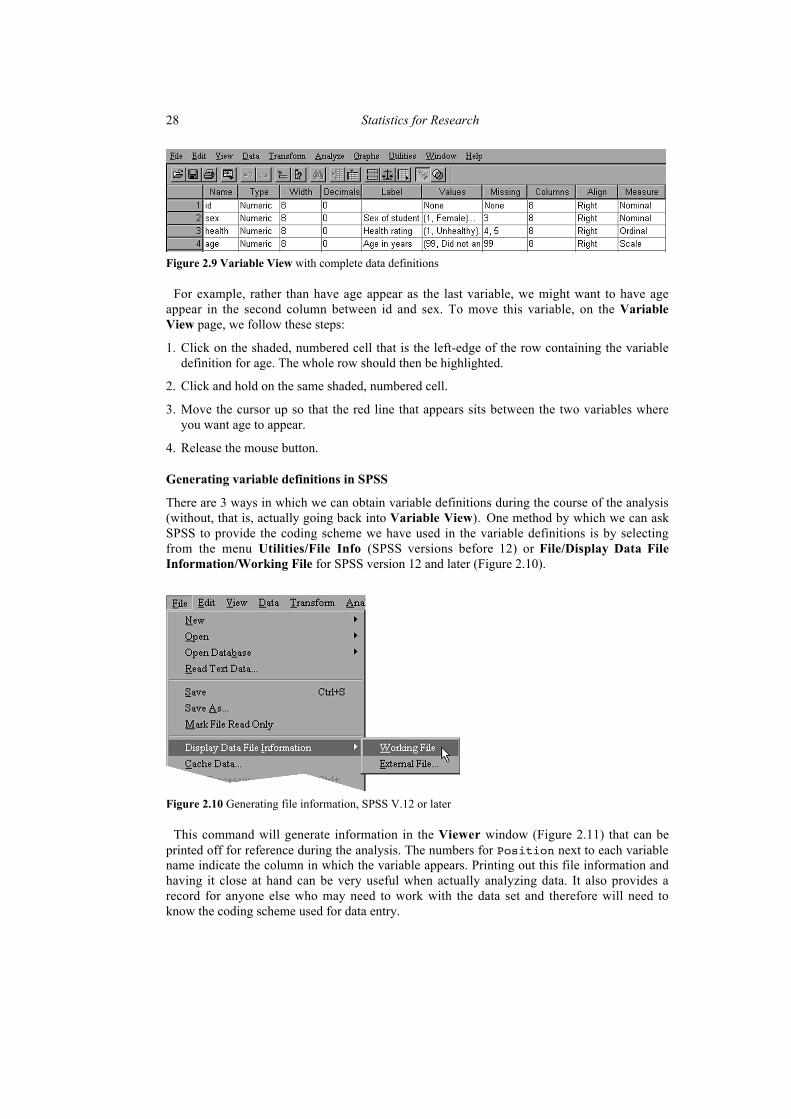
Generating variable definitions in SPSS

There are 3 ways in which we can obtain variable definitions during the course of the analysis(without, that is, actually going back into Variable View). One method by which we can askSPSS to provide the coding scheme we have used in the variable definitions is by selectingfrom the menu Utilities/File Info (SPSS versions before 12) or File/Display Data FileInformation/Working File for SPSS version 12 and later (Figure 2.10).

Figure 2.10 Generating file information, SPSS V.12 or later

This command will generate information in the Viewer window (Figure 2.11) that can beprinted off for reference during the analysis. The numbers for Position next to each variablename indicate the column in which the variable appears. Printing out this file information andhaving it close at hand can be very useful when actually analyzing data. It also provides arecord for anyone else who may need to work with the data set and therefore will need toknow the coding scheme used for data entry.


File Information

List of variables in the working file

Name (Position) Label

Id (1)Measurement Level: NominalColumn Width: Unknown Alignment: RightPrint Format: F8Write Format: F8

sex (2) Sex of studentMeasurement Level: NominalColumn Width: Unknown Alignment: RightPrint Format: F8Write Format: F8Missing Values: 3

Value Label1 Female2 Male3 M Did not answer

health (3) Health ratingMeasurement Level: OrdinalColumn Width: Unknown Alignment: RightPrint Format: F8Write Format: F8Missing Values: 4, 5

Value Label1 Unhealthy2 Healthy3 Very healthy4 M Don’t know5 M Did not answer

age (4) Age in yearsMeasurement Level: ScaleColumn Width: Unknown Alignment: RightPrint Format: F8Write Format: F8Missing Values: 99

Figure 2.11 SPSS File Info output

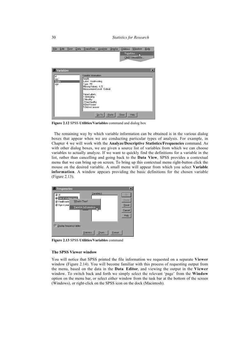
The File Info command allows you to obtain variable definitions for all your variables atonce. You may, however, occasionally want to quickly obtain the definition for one variableon the screen. This can be done through the Utilities/Variables command. This commandwill bring up the Variables dialog box, from which you can select the variable for whichdefinitions are required (Figure 2.12).

The Utilities/Variables command provides one additional function, which is speciallyuseful when working with large data files with lots of variables. Say I want to find out whatthe response to variable age is for case number 15 in a particular data set. If I select the rowcontaining the data for case number 15, and in the Variables dialog box then select age andclick on the Go To button, the active cell will jump to the one containing this particulardatum. This eliminates the need to scroll across and down a large file of numbers which caneasily blend into each other and make it difficult to find the particular entry we are trying tolocate.


Figure 2.12 SPSS Utilities/Variables command and dialog box

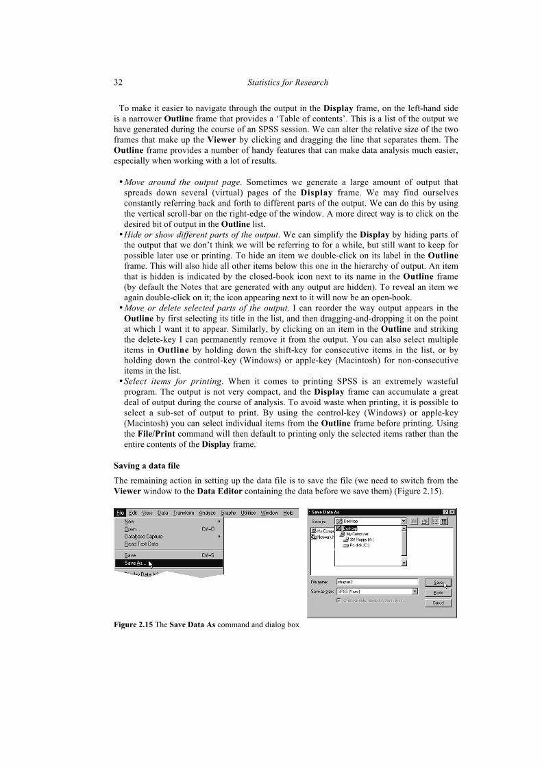
The remaining way by which variable information can be obtained is in the various dialogboxes that appear when we are conducting particular types of analysis. For example, inChapter 4 we will work with the Analyze/Descriptive Statistics/Frequencies command. Aswith other dialog boxes, we are given a source list of variables from which we can choosevariables to actually analyze. If we want to quickly find the definitions for a variable in thelist, rather than cancelling and going back to the Data View, SPSS provides a contextualmenu that we can bring up on screen. To bring up this contextual menu right-button click themouse on the desired variable. A small menu will appear from which you select Variableinformation. A window appears providing the basic definitions for the chosen variable(Figure 2.13).

Figure 2.13 SPSS Utilities/Variables command

The SPSS Viewer window

You will notice that SPSS printed the file information we requested on a separate Viewerwindow (Figure 2.14). You will become familiar with this process of requesting output fromthe menu, based on the data in the Data Editor, and viewing the output in the Viewerwindow. To switch back and forth we simply select the relevant ‘page’ from the Windowoption on the menu bar, or select either window from the task bar at the bottom of the screen(Windows), or right-click on the SPSS icon on the dock (Macintosh).


Figure 2.14 The SPSS Viewer window

The major part of the Viewer window is a Display frame that contains the information wehave requested. Two points are worth noting about the Display:

• SPSS does not print over existing output whenever we request new information. Instead itadds new output to the bottom of the existing output. When undertaking a lot of analysisthis can create a lengthy Display.• ‘Old’ output is not automatically updated whenever we change information on the Data

Editor window. For example, if we went back and changed the value labels for thevariables we are working with, the variable information we have just generated will nolonger apply, but will still be recorded on the Viewer window. We will need to again runthe File Info command to generate the information for the updated variable labels.

It is often very helpful to add text to explain the output listed in the Display. For example,the file information we generated just states File Information as a title. You can double-clickon this title (or any other text in the Display) and add/change the text, or also change theformatting. Thus you may add text to the title so that it reads File Information for Ch.02.savso that when you print this output you know to which data file it applies. Alternatively, youcan use the Insert command to insert particular types of preformatted text into the output. Theoptions available for adding new text (rather than editing existing text) are:

• New Heading. This appears in the navigator window and acts like a new heading in a Tableof Contents.• New Title. This is a first-level heading that normally appears in large, bold font.• New Page Title. A page-break is automatically inserted before a page title, and the typed

text appears at the top-center of the page.• New Text. This is small, plain text.


To make it easier to navigate through the output in the Display frame, on the left-hand sideis a narrower Outline frame that provides a ‘Table of contents’. This is a list of the output wehave generated during the course of an SPSS session. We can alter the relative size of the twoframes that make up the Viewer by clicking and dragging the line that separates them. TheOutline frame provides a number of handy features that can make data analysis much easier,especially when working with a lot of results.

• Move around the output page. Sometimes we generate a large amount of output thatspreads down several (virtual) pages of the Display frame. We may find ourselvesconstantly referring back and forth to different parts of the output. We can do this by usingthe vertical scroll-bar on the right-edge of the window. A more direct way is to click on thedesired bit of output in the Outline list.• Hide or show different parts of the output. We can simplify the Display by hiding parts of

the output that we don’t think we will be referring to for a while, but still want to keep forpossible later use or printing. To hide an item we double-click on its label in the Outlineframe. This will also hide all other items below this one in the hierarchy of output. An itemthat is hidden is indicated by the closed-book icon next to its name in the Outline frame(by default the Notes that are generated with any output are hidden). To reveal an item weagain double-click on it; the icon appearing next to it will now be an open-book.• Move or delete selected parts of the output. I can reorder the way output appears in the

Outline by first selecting its title in the list, and then dragging-and-dropping it on the pointat which I want it to appear. Similarly, by clicking on an item in the Outline and strikingthe delete-key I can permanently remove it from the output. You can also select multipleitems in Outline by holding down the shift-key for consecutive items in the list, or byholding down the control-key (Windows) or apple-key (Macintosh) for non-consecutiveitems in the list.• Select items for printing. When it comes to printing SPSS is an extremely wasteful

program. The output is not very compact, and the Display frame can accumulate a greatdeal of output during the course of analysis. To avoid waste when printing, it is possible toselect a sub-set of output to print. By using the control-key (Windows) or apple-key(Macintosh) you can select individual items from the Outline frame before printing. Usingthe File/Print command will then default to printing only the selected items rather than theentire contents of the Display frame.

Saving a data file

The remaining action in setting up the data file is to save the file (we need to switch from theViewer window to the Data Editor containing the data before we save them) (Figure 2.15).

Figure 2.15 The Save Data As command and dialog box


We need to decide where we want to store the file. This is usually a choice betweensomewhere on the computer’s hard drive, or on a disk that we place in the disk drive.Wherever you choose to store data it is very important to make a regular backup. No storagemedium is immune to errors. Get into the habit of making a copy of your data files to guardagainst any unforeseeable problems.

Once this has been done the name of the active data file will appear in the bar at the top ofthe Data Editor (Figure 2.16).

Figure 2.16 SPSS File name display

After using the File/Save As command, a file can be quickly resaved in the same location andwith the same name with the File/Save command instead of File/Save As. In fact, you shouldnot wait until the end of your data entry session to save the file. Mishaps can happen, often atthe worst time. Losing data, after spending a considerable amount of time entering them, canbe very demoralizing. We should get into the habit of saving work every 15 minutes or so(and also making a backup).

Data entry

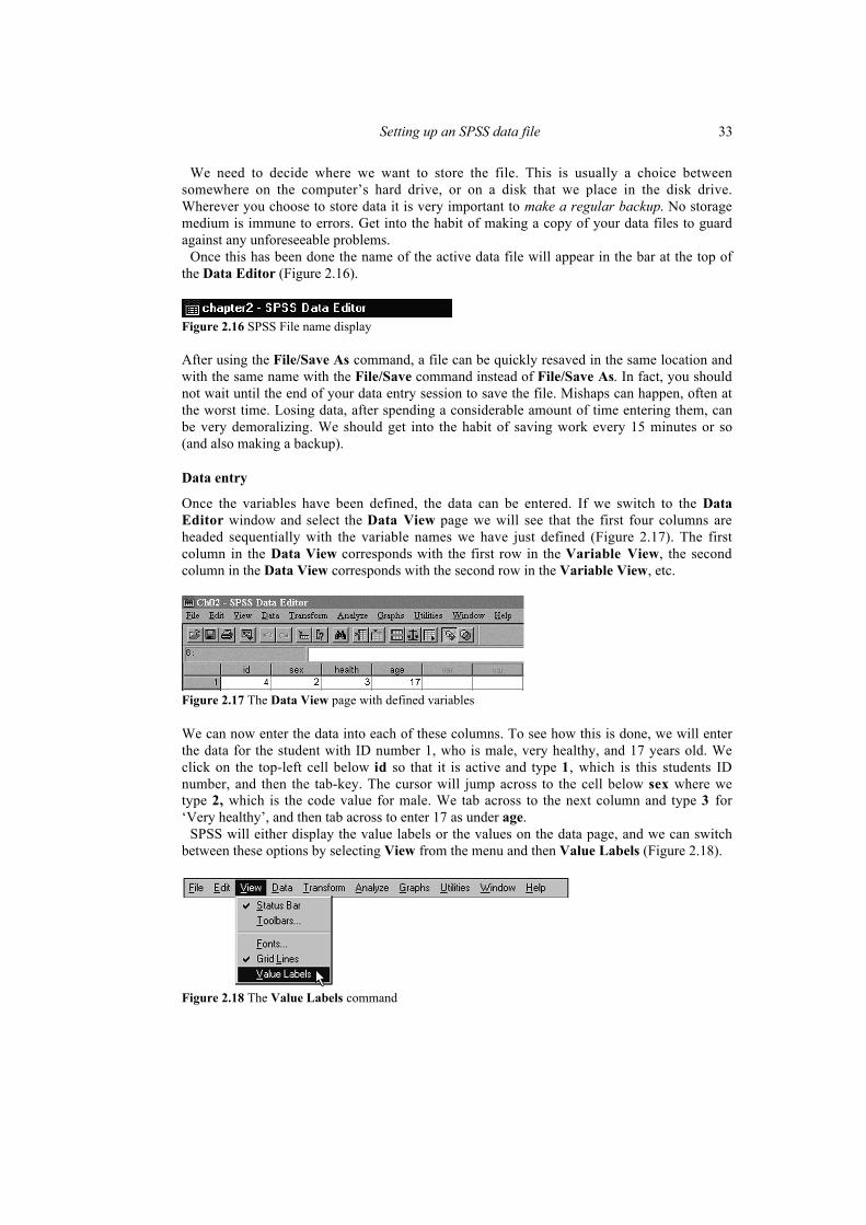
Once the variables have been defined, the data can be entered. If we switch to the DataEditor window and select the Data View page we will see that the first four columns areheaded sequentially with the variable names we have just defined (Figure 2.17). The firstcolumn in the Data View corresponds with the first row in the Variable View, the secondcolumn in the Data View corresponds with the second row in the Variable View, etc.

Figure 2.17 The Data View page with defined variables

We can now enter the data into each of these columns. To see how this is done, we will enterthe data for the student with ID number 1, who is male, very healthy, and 17 years old. Weclick on the top-left cell below id so that it is active and type 1, which is this students IDnumber, and then the tab-key. The cursor will jump across to the cell below sex where wetype 2, which is the code value for male. We tab across to the next column and type 3 for‘Very healthy’, and then tab across to enter 17 as under age.

SPSS will either display the value labels or the values on the data page, and we can switchbetween these options by selecting View from the menu and then Value Labels (Figure 2.18).

Figure 2.18 The Value Labels command


The advantage of viewing data as labels rather than numeric codes is that when we enterdata that have been assigned value labels into a cell, we are presented with a contextual menufrom which we can select the appropriate response. For example, to enter the fact that Case 1is male, we can either type 2, or click on the down-arrow in the cell and scroll to Male in thelist.

You may notice that, as you type, the data initially appear on the bar just above the datafields, called the Cell Editor (Figure 2.19).

Figure 2.19 The Cell Editor

This is where information is entered until you hit the tab key, which then enters the data intothe active cell. The ‘address’ of the active cell is indicated on the left of the Cell editor. Thisaddress is defined by the combination of the row number and column name that intersect atthe active cell. If at any point we make a mistake, or we need to change the information in anyparticular cell, we simply make that cell active and type in the new information. On hitting thereturn key the new value will replace the old.

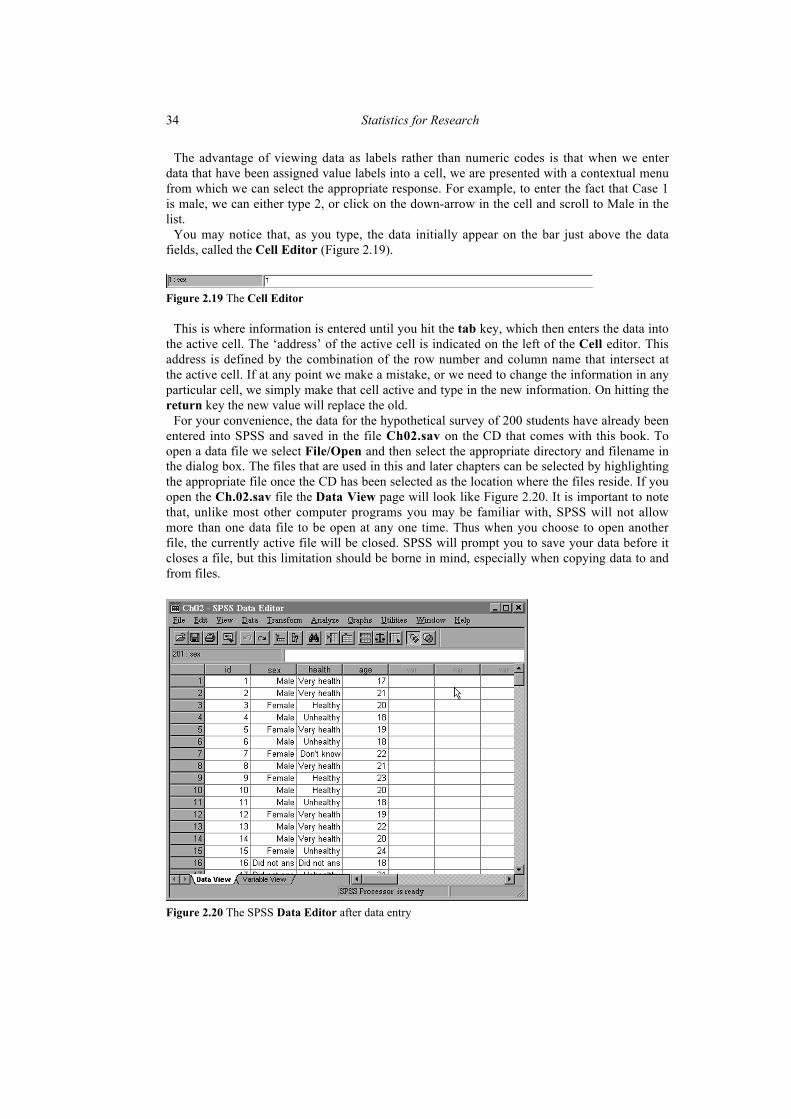
For your convenience, the data for the hypothetical survey of 200 students have already beenentered into SPSS and saved in the file Ch02.sav on the CD that comes with this book. Toopen a data file we select File/Open and then select the appropriate directory and filename inthe dialog box. The files that are used in this and later chapters can be selected by highlightingthe appropriate file once the CD has been selected as the location where the files reside. If youopen the Ch.02.sav file the Data View page will look like Figure 2.20. It is important to notethat, unlike most other computer programs you may be familiar with, SPSS will not allowmore than one data file to be open at any one time. Thus when you choose to open anotherfile, the currently active file will be closed. SPSS will prompt you to save your data before itcloses a file, but this limitation should be borne in mind, especially when copying data to andfrom files.

Figure 2.20 The SPSS Data Editor after data entry


Checking for incorrect values: Data cleaning

Whether we enter data into SPSS ourselves or receive data from other people, before weactually analyze the data, we need to check that the data are ‘clean’. Clean data are data thatdo not contain any invalid or nonsensical values e.g. we don’t have someone with an age of234 years, or someone coded 3 for sex, when we have coded ‘females = 1’ and ‘males = 2’.

We check data to see if they need cleaning by generating frequency tables on all thevariables (see Chapter 4). Frequency tables allow us to check to see that there are no valuesthat are outside the permissible range. We can also use more elaborate analysis such ascrosstabulations to assess whether particular groups within the data set only have values thatare valid for them.

If we discover unusual responses during the data cleaning process, we make either of thefollowing changes to the data set:

• if it is a data entry mistake, go back to the original data gathering instrument for that case,by cross-referencing the id number, and find the appropriate value to enter; or• if it is an invalid response, type in an assigned missing value.

Summary

We have worked through the process of setting up an SPSS data file. Needless to say we haveonly skimmed the surface with respect to the full range of options available. I leave it to thereader to play around with SPSS and learn the full range of features that it provides. Theprogram comes with its own tutorial and sample data files that will guide you through thevarious features. The program also comes with a very useful help facility, which is availablefrom the menu bar. In addition, the CD that accompanies this book includes a number of extrachapters that illustrate some of the more advanced functions available in SPSS. These includethe Recode command, the Multiple Response command, the Compute command, and theSelect Cases command.

One last point needs to be made about working with SPSS. Many of the default settings forentering, presenting, and analyzing data in SPSS are less than ideal. For example, displayingnumeric data by default to 2 decimal places is annoying when most data are entered in wholenumbers. This does not actually affect any results, but makes the Data View pageunnecessarily cluttered. The Decimals setting on the Variable View page can be changedwhenever we work with a new file as we described above. An alternative is to use theEdit/Options (Windows) or the SPSS/Preferences (Macintosh) command to change thedefault setting once and for all, so that when data are entered they appear with 0 decimalplaces (i.e. whole numbers). The settings that can be changed under this command are far toonumerous to even list here; you should explore these at your leisure, but with one word ofwarning: do not alter the default setting on someone else’s version of SPSS without theirpermission.

Exercises

2.1 A survey gathers the data for the weekly income of 20 people, and obtains thefollowing results:

$0, $0, $250, $300, $360, $375, $400, $400, $400, $420, $425, $450, $462, $470,$475, $502, $520, $560, $700, $1020

Create an SPSS data file and enter these data, entering all the necessary labels. Savethe file with an appropriate filename.


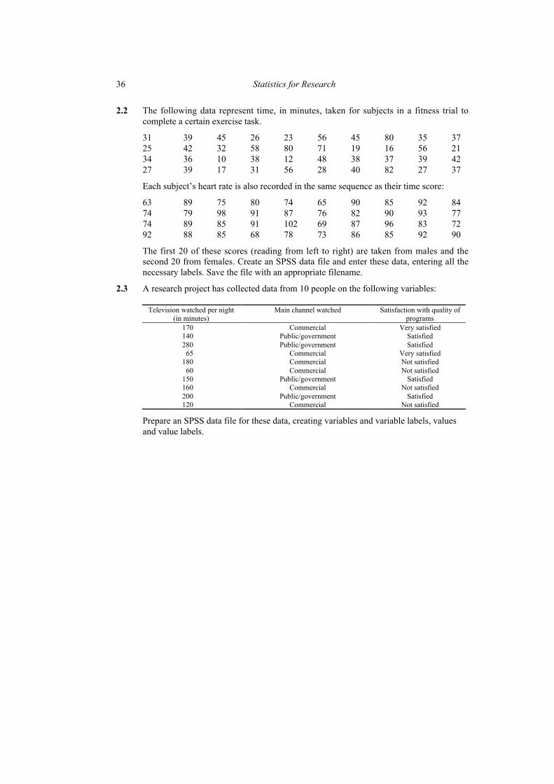
2.2 The following data represent time, in minutes, taken for subjects in a fitness trial tocomplete a certain exercise task.

31 39 45 26 23 56 45 80 35 3725 42 32 58 80 71 19 16 56 2134 36 10 38 12 48 38 37 39 4227 39 17 31 56 28 40 82 27 37

Each subject’s heart rate is also recorded in the same sequence as their time score:

63 89 75 80 74 65 90 85 92 8474 79 98 91 87 76 82 90 93 7774 89 85 91 102 69 87 96 83 7292 88 85 68 78 73 86 85 92 90

The first 20 of these scores (reading from left to right) are taken from males and thesecond 20 from females. Create an SPSS data file and enter these data, entering all thenecessary labels. Save the file with an appropriate filename.

2.3 A research project has collected data from 10 people on the following variables:

Television watched per night(in minutes)

Main channel watched Satisfaction with quality ofprograms

170 Commercial Very satisfied140 Public/government Satisfied280 Public/government Satisfied

65 Commercial Very satisfied180 Commercial Not satisfied

60 Commercial Not satisfied150 Public/government Satisfied160 Commercial Not satisfied200 Public/government Satisfied120 Commercial Not satisfied

Prepare an SPSS data file for these data, creating variables and variable labels, valuesand value labels.

Documents

Setting up an SPSS data file - SAGE Publications · Setting up an SPSS data file This chapter will introduce SPSS, ... statistics package (other than common spreadsheet programs such