1

Setting Parameters for Simulated

Annealing

• All heuristic algorithms (and many nonlinear

programming algorithms) are affected by

“algorithm parameters”

• For Simulated Annealing the algorithm

parameters are

• To, M, , , maxtime

• So how do we select these parameters to make

the algorithm efficient?

Handout for videotaped lecture labeled 9-2-11 (taped after regular lecture on 9-2-11)

22

Setting Parameters in Simulated

Annealing

• As we saw in the first simulated annealing

problem, the results can depend a great deal on

the values of the parameter T (“temperature”),

which depends upon To and upon α.

• How should we pick To and α?

• We can use some simple procedures to pick

estimate a reasonable value (not necessarily

optimal) of To .

– user decides on the probability of P1 of accepting

an uphill move initially and P2 the probability of

accepting an uphill move after G iterations.

3

Rough Estimates for Good Algorithm

Parameter Values

• Note that the best algorithm parameters cannot be determined exactly and that the results are probably not sensitive to small changes in algorithm parameter values.

• Recall in previous SA example there was a difference between a To of 100 and a To of 500 in the two examples. This is a difference of 500% in the algorithm parameter value-not a small change.

• Hence you are trying to get a rough estimate of what would be good algorithm parameter values .

BOARD : change in search over time

• (stop here)

0 G MaxTime

allow uphill moves(not greedy) (greedy)

Numbers of objective function evaluations

4

55

Simple Approach to Parameterizing SA

• Assume M=1

• Assume – you want to do Maxtime iterations and you want

Maxtime-G of these to be greedy. (Here greedy means having a probability of less than P2 for uphill move.)

– The estimated range of values of Cost(S) = R

– R= Max Cost (S)-Min Cost (S)

– Initially you want to accept P1 fraction of the moves.

– By the time you have done G iterations you want to have an essentially greedy search and accept P2 or fewer fraction of the moves.

– P2<<P1 (For example, P1=.95 and P2 = .01)

66

Selecting Algorithm Parameters

• So how do we select these parameters to make the algorithm efficient?

• Recall that the principle is that initially you want to accept a relatively high percentage of uphill moves (for a minimization problem), but the more iterations you have done, the less you want to accept uphill moves.

• Acceptance of uphill moves is determined by To, M, and . Assume M = 1, then Ti = i To

starting with T= To.

Let P1 be your goal for the average probability of accepting an UPHILL move initially and P2 be your goal for the probability of accepting an Uphill move after G iterations.

7

Simulated Annealing Morphs into What?

• Intially Simulated Annealing has a

significant probability of accepting an uphill

move.

• After many interations, Simulated

Annealing becomes similar to what

algorithm (Random Walk, Random

Sampling, or Greedy Search)? Why?

88

Given To,, Select α

• Once αi gets small enough after i iterations, then

SA operates like ________search. WHY?

• You have maxtime as the maximum number of

iterations.

• Decide what fraction of these you want to have

spent in greedy search.

• Let G= maxtime- number of iterations for greedy

search and let P2>0, be a small number that

allows very few uphill movements. (P2 selected

by user)

99

BOARD P is probability of acceptance of

uphill move

Number of iterations

maxiter

10

Effect of iteration number i on Probability

• After i iterations, T= αi To.(Decreasing)

• We know that P decreases as T

decreases. Thus,

P

Iteration i

Pick the number of iterations G when you

want the probability of acceptance to be a

low P2.

maxtime

1111

Simple Method for Setting To

• Estimate the average of ΔCost. (called avgΔCost) for uphill moves in the initial iteration.

We will discuss later ways to estimate this.

• Decide that you want initially to allow approximately Po percent of the uphill moves to Snew moves to be accepted. (User decision)

• Then given Po and avgΔCost, can you give an equation that includes To?

is approximately what you want, and you can solve for To. So To =(-avgCost)/(ln P1)

Estimate for α

• Recall that our estimates for To and α are rough estimates of what would be good values, i.e. within an order of magnitude.

• To estimate a good value for α, we need to consider how fast do we want the probability of accept an uphill move to decline.

• We define this by the user deciding what probability (P2) do you want after G iterations.

• Recall Simulated annealing becomes like Greedy Search if the probability of uphill moves gets small and this probability is determined by α g To after g iterations.

13

Selecting a value for α• The probability P in kth iteration of accepting uphill

move is

Pk = exp(-[COST(NewS)-COST(CurS)]/Tk

We also have

Tk= Tk-1 α = (Tk-2 α) α= ….=To αk

(The lower numbers are subscripts for iteration number. However the upper k on α is an exponential power). So the term that appears in the probability equation in the Gth iteration is

P2 = exp(-[COST(NewS)-COST(CurS)]/[αG To ])

P2 approximately =exp(-[avg ΔCOST)/[αG To ])

If we have already computed To, and we are given P2, G and avgΔCOST .

Hence we can compute α.

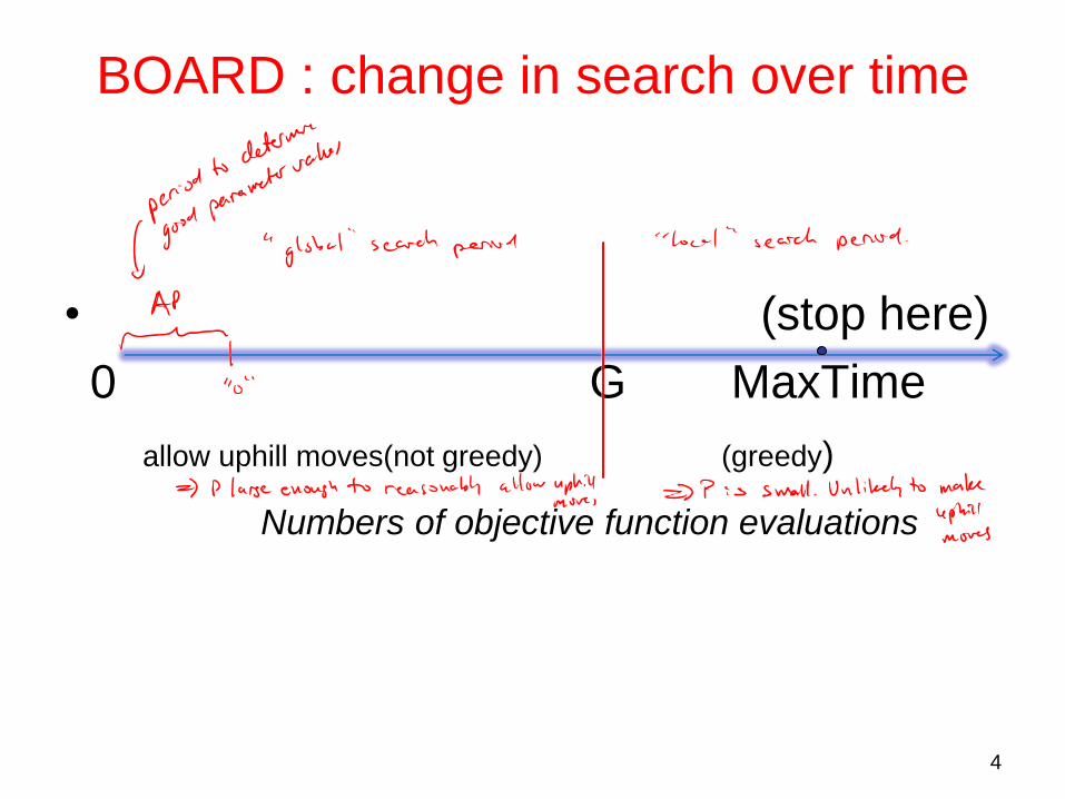
Selecting α

14

After G iterations and average ΔCost,

T=αG To,

so we compute the appropriate value of α

using the equations on the following slide.

Recall P2 is the probability of accepting an

uphil move after G interation. If we assume

average Δcost (=“avgCost” for short) then

15

2 exp( / )P avgCost T

02 exp( / )GP avgCost T

0ln 2 ln exp( / )GP avgCost T

0/ ln 2G avgCost T P

0ln 2 / GP avgCost T

1/

0( / ( ln 2)) GavgCost T P

Computing α , Given To , P2 and G

Previous handwritten slide in videotaped lecture erroneously had “log” instead of “ln”