Embed Size (px)
Citation preview

SETOFF Version 3.0
Ensoft, Inc. Engineering Software. 2011
3003 W. Howard Lane Austin, Texas 78728 Phone: (512) 244-6464 Fax: (512) 244-6067 www.ensoftinc.com
COPYRIGHT ENSOFT, INC 2011 NO REPRODUCTION OR DISTRIBUTION WITHOUT AUTHORIZATION FROM ENSOFT, INC

Contents CHAPTER 1. Introduction ................................................................................................................... 1-1
1.1 Introduction ............................................................................................................................... 1-2
1.2 Organization ............................................................................................................................... 1-2
1.3 Capabilities of Program Setoff ................................................................................................... 1-2
1.4 General Concepts ....................................................................................................................... 1-2
1.5 Use of the Program .................................................................................................................... 1-3
CHAPTER 2. Installation and Getting Started ..................................................................................... 2-1
2.1 Standard Installation Procedures ............................................................................................... 2-2
2.2 Network Versions ....................................................................................................................... 2-4
2.2.1 General Description ........................................................................................................... 2-4
2.2.2 Installation of Network Version ......................................................................................... 2-4
2.3 Software Updates on the Internet ............................................................................................. 2-6
2.4 Installation of Software Updates ............................................................................................... 2-6
2.5 Getting Started ........................................................................................................................... 2-7
2.5.1 Starting the Program .......................................................................................................... 2-7
2.5.2 File Management ............................................................................................................... 2-7
2.5.3 File Management ............................................................................................................... 2-9
2.5.4 Data Input of Application Problem .................................................................................... 2-9
2.5.5 Options Menu .................................................................................................................. 2-10
2.5.6 Computation Options ....................................................................................................... 2-10
2.5.7 View Options .................................................................................................................... 2-10
2.5.8 Show Options ................................................................................................................... 2-10
2.5.9 Arrangement of Windows ................................................................................................ 2-11
2.5.10 Help Files .......................................................................................................................... 2-11
CHAPTER 3. References for Data Input .............................................................................................. 3-1
3.1 File Menu ................................................................................................................................... 3-2
3.1.1 File - New ........................................................................................................................... 3-2
3.1.2 File - Open .......................................................................................................................... 3-2
3.1.3 File - Save ........................................................................................................................... 3-2
3.1.4 File - Save As ....................................................................................................................... 3-2
COPYRIGHT ENSOFT, INC 2011 NO REPRODUCTION OR DISTRIBUTION WITHOUT AUTHORIZATION FROM ENSOFT, INC

3.1.5 File - Save Bitmap ............................................................................................................... 3-2
3.1.6 File – Print .......................................................................................................................... 3-2
3.1.7 File - Exit ............................................................................................................................. 3-4
3.2 Data Menu ................................................................................................................................. 3-4
3.2.1 Numeric Data Entries ......................................................................................................... 3-4
3.2.2 System of Units .................................................................................................................. 3-5
3.2.3 Data - Title .......................................................................................................................... 3-5
3.2.4 Data - Soil Layer Data ......................................................................................................... 3-6
3.2.5 Types of Compressibility Curves ........................................................................................ 3-7
3.2.6 Data - Soil Compressibility Curves ................................................................................... 3-10
3.2.7 Data – Settlement Points Data ......................................................................................... 3-11
3.2.8 Data – Foundation Configuration .................................................................................... 3-12
3.2.9 Data – Loaded Shallow Footings Area data ..................................................................... 3-12
3.2.10 Data – Pile Foundation Data ............................................................................................ 3-14
CHAPTER 4. References for Program Execution and Output Reviews ............................................... 4-1
4.1 Introduction ............................................................................................................................... 4-2
4.2 Computation Menu .................................................................................................................... 4-2
4.2.1 Computation – Run Analysis .............................................................................................. 4-2
4.2.2 Computation- Edit Input Text ............................................................................................ 4-2
4.2.3 Computation- View Output Text ........................................................................................ 4-3
4.3 View Menu ................................................................................................................................. 4-4
4.3.1 View – Graphics .................................................................................................................. 4-5
4.3.2 View – 3D View .................................................................................................................. 4-5
4.4 Show Menu ................................................................................................................................ 4-5
CHAPTER 5. Example Problems .......................................................................................................... 5-1
5.1 Introduction ............................................................................................................................... 5-2
5.2 Description of Output Tables ..................................................................................................... 5-2
5.3 Example 1 ................................................................................................................................... 5-3
5.3.1 Input Data .......................................................................................................................... 5-7
5.3.2 Output Results ................................................................................................................. 5-10
5.4 Example 2 ................................................................................................................................. 5-19
5.4.1 Problem Description ........................................................................................................ 5-19
COPYRIGHT ENSOFT, INC 2011 NO REPRODUCTION OR DISTRIBUTION WITHOUT AUTHORIZATION FROM ENSOFT, INC

5.4.2 Data Input ........................................................................................................................ 5-20
5.4.3 Computation Menu .......................................................................................................... 5-24
COPYRIGHT ENSOFT, INC 2011 NO REPRODUCTION OR DISTRIBUTION WITHOUT AUTHORIZATION FROM ENSOFT, INC

CHAPTER 1. Introduction
COPYRIGHT ENSOFT, INC 2011 NO REPRODUCTION OR DISTRIBUTION WITHOUT AUTHORIZATION FROM ENSOFT, INC

CHAPTER 1 Introduction 1-2
1.1 Introduction Welcome to the foundation settlement analysis program SETOFF (SETtlement Of Footing Foundations). This document and associated computer program provide methods to compute consolidation settlements at selected points due to the loads from foundations consisting of one or more footings and/or mats. Version 3.0 now includes computations for settlement of deep foundations. This program uses generally-accepted procedures to compute consolidation settlement for footing foundations.
1.2 Organization This user’s manual is divided into five chapters. Chapter 2 contains information for installation and running SETOFF 3.0 for Windows. Chapter 3 contains a detailed guide to prepare the input data required by the program SETOFF, and Chapter 4 contains instructions for running the program and presenting computed settlement and graphics plots. Chapter 5 contains a description of the output from the program SETOFF and the input and output for an example problem. Chapter 6 contains a description of the computational procedures used by SETOFF in sufficient detail so users could make the computations manually.
1.3 Capabilities of Program Setoff The program can be used to compute settlements at as many as 25 points due to the loading from as many as 50 footings and pile foundations with pile caps, represented as loaded areas. The soil stratigraphy includes up to 25 soil layers and as many as 10 soil compressibilities.
The loaded areas may be rectangular or circular in shape, and they may be included in the foundation in any order or combination. A loaded area may be placed at the ground surface or at any depth below the ground surface. The pressure applied to the soil by a loaded area may be positive, as for structural loads, or negative, representing soil excavation. The effect of all loaded areas is included in computing settlements in all soil layers beneath all settlement points. ???Settlement results are considered to be the final settlement in regards to consolidation as a time-dependant function???.
Soil compressibility can be represented by typical data from laboratory consolidation tests, either directly as received from the laboratory or in a modified form. The compressibility data can be entered either as a series of points for a nonlinear curve or as the slope of a linear soil compressibility curve.
1.4 General Concepts Settlement of structures supported on footings and mats was a mystery to designers and constructors for a long time. In 1925 Karl Terzaghi published his book Erdbaumechanik where an explanation of the settlement phenomenon was given. This initiated increased activity in the observation of actual structure settlement and in the development of computational procedures to predict such settlement. The computation of settlement for structures supported on soil-supported footings or mats has become an accepted procedure in geotechnical engineering.
Total settlement of a foundation is generally considered to consist of two parts, elastic and consolidation settlement. Elastic settlement occurs because of the pseudo-elastic nature of most soils and it occurs immediately on application of the foundation load. Consolidation settlement takes place as
COPYRIGHT ENSOFT, INC 2011 NO REPRODUCTION OR DISTRIBUTION WITHOUT AUTHORIZATION FROM ENSOFT, INC

CHAPTER 1 Introduction 1-3
the pore space in the soil is reduced under the foundation loading and it may require a period of time to be fully developed. The elastic settlement may not be important because it takes place during construction as the structural loads are added. Because of this, some compensation for the elastic settlement may take place during construction. This does not mean, however, that elastic settlement should be overlooked.
1.5 Use of the Program Computation of consolidation settlement may be divided into three parts. The first part is the determination of the soil stratigraphy and the representative properties of the soil in each stratum. The second part is the computation of the stress increase at pertinent points in the subsurface soils due to the foundation loading. The third part is the computation of settlement using the data from the first two parts. The computer program SETOFF will perform the latter two parts: computation of the stress increase and settlement.
The settlements computed by the program SETOFF will be only as good as the input data. The soil stratigraphy and soil properties should be determined by an adequate soil investigation conducted by a competent geotechnical engineer.
Settlement is very specific. The actual settlement observed in the field will depend on actual foundation loads and soil conditions and not on values assumed for design. The foundation loading used should be the actual sustained loads and not the maximum design loads. If the rebound from an excavation is to be computed, the input soil compressibility should adequately represent the action of the soil under reducing stress as well as increasing stress; this may not be the unmodified results from consolidation tests. If the computed settlement is borderline, it may be necessary for further analysis and interpretation of the output from program SETOFF by a competent engineer.
Although this program will permit computation of settlement for complex foundations that would be too tedious for manual calculation, it should not be used without the input from a person familiar with all aspects of the settlement process.
COPYRIGHT ENSOFT, INC 2011 NO REPRODUCTION OR DISTRIBUTION WITHOUT AUTHORIZATION FROM ENSOFT, INC

CHAPTER 2. Installation and Getting Started
COPYRIGHT ENSOFT, INC 2011 NO REPRODUCTION OR DISTRIBUTION WITHOUT AUTHORIZATION FROM ENSOFT, INC

CHAPTER 2 Installation and Getting Started 2-2
2.1 Standard Installation Procedures Program SETOFF 3.0 is distributed in a CD ROM along with its User’s Manual, and a security device. The software will only be functional in computers that have the security device, or hardware lock, attached to their parallel port.
Besides SETOFF 3.0, the distribution CD ROM contains many other software programs that are produced by ENSOFT. However, these additional software programs will only run in evaluation mode unless the proper hardware lock is connected and operating.
The user is assumed to have a basic knowledge for running applications under Windows. The following steps are recommended for a successful installation of the software version for single users.
1.) The hardware lock must be attached to the computer before installing the software. To prevent problems to the electrical circuitry of the computer in use, the manufacturer of the hardware locks recommends the following optimum guidelines to install the devices:
• Turn off computer power to avoid any possibility of damage to the electrical circuitry of the computer in use.
• Make sure that the I/O card is firmly seated on the motherboard.
• Remove the printer cable from local computer, if attached.
• Install the hardware lock with its male end towards the computer.
• Reconnect the printer cable to the hardware lock, if the cable was previously attached to the local computer.
2.) Start Windows. 3.) Insert the Ensoft CD ROM in the appropriate tray and slide the tray back into the computer.
COPYRIGHT ENSOFT, INC 2011 NO REPRODUCTION OR DISTRIBUTION WITHOUT AUTHORIZATION FROM ENSOFT, INC

CHAPTER 2 Installation and Getting Started 2-3
Fig. 2.1 Main installation screen for ENSOFT software
4.) In most computers the main installation program will start automatically a few seconds after the CD tray is pushed back into the computer. If not started automatically, users should click on the Start button, select Run, and type x:\setup.exe, where x represents the drive which contains the Ensoft CD. Press e or click OK to execute the command and start the main installation program.
The graphics layout of the main installation interface for ENSOFT’s programs is shown in Figure 2.1. The actual layout during the user’s installation may be different than Fig. 2.1, since the installation interface is updated regularly and Fig. 2.1 only represents the screen at the time of writing of this manual.
5.) To install the standard (single user) version of SETOFF 3.0 users should click the SETOFF 3.0 icon and select the Install Standard button.
COPYRIGHT ENSOFT, INC 2011 NO REPRODUCTION OR DISTRIBUTION WITHOUT AUTHORIZATION FROM ENSOFT, INC

CHAPTER 2 Installation and Getting Started 2-4
6.) Users will be provided with an option to select a drive and directory for installing SETOFF 3.0; the default is c: \ensoft\setoff3. If the desired directory does not exist, the installation program will automatically create a new directory in the chosen hard drive.
7.) In some cases, users may be requested to reboot Windows before executing the program. Users may run the program by double-clicking its icon in the SETOFF3 folder.
A detailed description of the registry changes performed to the operating system is contained in the readme_???95-98. txt, and readme_nt. txt files installed in the chosen SETOFF 3 directory. The exact destination of system files and software drivers are also described in those installation files.
2.2 Network Versions Special network licenses and hardware locks are avail-able from ENSOFT, INC. if users desire to operate SETOFF 3.0 on a Windows network. The network version is limited to users with two or more licenses at the same physical site. Discounted rates apply for users purchasing multiple licenses for the same site.
2.2.1 General Description Network versions of SETOFF 3.0 have special subroutines written for installations in “software servers” and for installations of “individual clients.”
The “software server” is known as the computer that will be carrying the network lock provided by ENSOFT, INC. The software server is not necessarily the same as the existing network server. Any computer in the existing Windows network may be designated software server for SETOFF 3 as long as the network lock is attached to its parallel port and the “server” version of the software is installed in its hard drive.
Software “clients” may be all other computers of the network that have the program installed as clients. Software clients do not need any hardware lock attached to their parallel port. The program installed in “software clients” will be allowed to run as long as the computer designated as “software server” is running on the network with the proper operating system and with its network lock secured in place.
Users of the network version of SETOFF 3 are allowed to have the software installed in as many computers as they have on their Windows network. However, only a number of users equal to the total number of purchased licenses (minimum two for networks) will be able to operate the program at the same time.
2.2.2 Installation of Network Version To install this program, the user must have administrative privileges to modify the Windows registry. In large computer networks, this is usually only available to network administrators. They are the ones recommended to proceed with these installations.
COPYRIGHT ENSOFT, INC 2011 NO REPRODUCTION OR DISTRIBUTION WITHOUT AUTHORIZATION FROM ENSOFT, INC

CHAPTER 2 Installation and Getting Started 2-5
1.) The network administrator must first define the computer that will be carrying the network lock for this software. The computer carrying the network lock is known as the "server" for this particular computer program. Notice that the "server" may be any computer in the network, and not necessarily the existing file server or network server.
2.) INSTALLATION TO A "SERVER": Attach the network lock to any parallel port of the software server. The "server" computer must be turned on and logged into the network to enable other users (ie, "clients") to access this computer program. To prevent problems to the electrical circuitry of the computer in use, the manufacturer of the hardware locks recommends the following optimum guidelines to install the devices:
• Turn off the computer power to avoid any possibility of damage to the electrical circuitry. • Make sure that the I/O card is firmly seated on the motherboard. • Remove the printer cable from local computer, if attached. • Install the hardware lock with its male end towards the computer. • Reconnect the printer cable to the hardware lock, if the cable was previously attached to the local computer.
3.) INSTALLATION TO "CLIENTS": It is not necessary to connect the network lock to client computers during installation nor during program executions. Once the program is executed, the installed network protocols will automatically recognize the computer where the network lock is residing and the number of simultaneous users.
4.) Start Windows.
5.) Insert the Ensoft CD ROM in the appropriate tray and slide the tray back into the computer.
In most computers the main installation program will start automatically a few seconds after the CD tray is pushed back into the computer. If not started automatically, users should click on the Start button, select Run, and type x:\setup.exe, where x represents the drive which contains the Ensoft CD. Press e or simply click OK to execute the command and start the main installation program.
The graphics layout of the main installation interface for ENSOFT programs was previously shown in Figure 2.1. The actual layout during the user’s installation may be different than Fig. 2.1, since the installation interface is updated regularly and Fig. 2.1 only represents the screen at the time of writing of this manual.
To install the network version of SETOFF 3.0 users should click the SETOFF 3.0 icon and select the Install Network button.
6.) Users will be prompted to select an installation to a "Client" or to a "Server" computer. If desired, the network administrator may install the program to a single directory in a "file server.” In this case, the software must first be installed in the file server as a “software server”
COPYRIGHT ENSOFT, INC 2011 NO REPRODUCTION OR DISTRIBUTION WITHOUT AUTHORIZATION FROM ENSOFT, INC

CHAPTER 2 Installation and Getting Started 2-6
and icons pointing to the studio.exe file (residing in the server) can later be created in each individual client computer.
Users will also be provided with an option to select a drive and directory for installing SETOFF 3.0; the default is c: \ensoft\setoff3. If the desired directory does not exist, the installation program will automatically create a new directory in the chosen hard drive.
7.) In some cases, users may be requested to reboot Windows before executing the program. Users may run the program by double-clicking its icon in the SETOFF3 folder.
A detailed description of the registry changes performed to the operating system is contained in the readme_???95-98. txt, and readme_nt. txt files installed in the chosen SETOFF 3 directory. The exact destination of system files and software drivers are also described in those installation files.
2.3 Software Updates on the Internet Occasionally, ENSOFT will produce minor software improvements and/or fixes and place the latest software programs on ENSOFT’s internet site. Users may freely download the latest program updates while browsing ENSOFT’s websites (www.ensoftinc.com and/or www.ensoft.net).
Users may also directly access the latest version of SETOFF 3.0 typing the following direct links in their Internet browser of choice (notice that all letters must be in lowercase):
Single-User Versions:
http://www.ensoftinc.com/updates/so2-32s.exe
Network Versions:
http://www.ensoftinc.com/updates/so2-32n.exe
Once accessed with their browsers, users must select to save the file to their local hard drive before installation is started. Software updates available on ENSOFT’s websites are actually full versions of the programs that have been compressed into single files to speed up the file downloads.
2.4 Installation of Software Updates 1.) Download the single file containing the software update and save to a local hard drive. 2.) Double click the downloaded file using Windows Explorer or click on the Start button, select
Run, and select to Browse to the location in your hard drive where the downloaded file was stored. Press e or simply click OK to execute the command and start decompressing the downloaded file.
COPYRIGHT ENSOFT, INC 2011 NO REPRODUCTION OR DISTRIBUTION WITHOUT AUTHORIZATION FROM ENSOFT, INC

CHAPTER 2 Installation and Getting Started 2-7
3.) An introductory message explains that files will be decompressed to a temporary directory (\windows\temp) and later re-moved after installation is completed. Users should click OK in the introductory screen and also click on Setup in the following screen in order to start decompressing files.
4.) Installation is started automatically after all files are decompressed. Users will be provided with an option to select a drive and directory for installing SETOFF 3.0; the default is c:\ensoft\setoff3. If the desired directory does not exist, the installation program will automatically create a new directory in the chosen hard drive. If the desired directory already exists, only the distribution files of SETOFF 3 will be replaced (executables, drivers, and example files). Data files created by the users should be left unchanged.
5.) In some cases, users may be requested to reboot Windows before executing the program. Users may run the program by double-clicking its icon in the SETOFF 3 folder.
2.5 Getting Started A general diagram showing the menu choices and operational flow chart of program SETOFF 3.0 is presented in Fig. 2.2. The following paragraphs provide a short description of the operational features of SETOFF 3.0 and should quickly enable the user to get started with the program.
2.5.1 Starting the Program The program is started by double clicking the left mouse button anywhere in the SETOFF 3.0 icon. A new window will appear on the screen, with the following top-menu choices: File, Data, Options, Computation, View, Window, and Help.
2.5.2 File Management The File menu option contains several submenus, as shown in Fig. 2.3; they are:
• New: to create a new data file.
• Open: to open an existing data file.
• Save: to save input data under the current file name.
• Save As: to save input data under a different file name.
• Exit : to exit program SETOFF 3.0.
Several additional files are created in every new SETOFF 3.0 run. A general description of these files is presented in Table 2.1. In general, every successful run of SETOFF 3.0 generates four text files in the same drive and directory where the input-data file was saved or opened. Any of these files may be
COPYRIGHT ENSOFT, INC 2011 NO REPRODUCTION OR DISTRIBUTION WITHOUT AUTHORIZATION FROM ENSOFT, INC

CHAPTER 2 Installation and Getting Started 2-8
opened with standard text editors or word-processing programs.
Fig. 2.2 Sample organization and operational flow chart
COPYRIGHT ENSOFT, INC 2011 NO REPRODUCTION OR DISTRIBUTION WITHOUT AUTHORIZATION FROM ENSOFT, INC

CHAPTER 2 Installation and Getting Started 2-9
Table 2.1
File Name Usage Description File Format Example Files
filename.set Input Data Text file nsetex1.set nsetex2.set
filename(Input Report).txt Input Report Text file nsetex1 (Input Report).txt nsetex2 (Input Report).txt
filename (Output Report).txt Output Report Text file nsetex1 (Output Report).txt nsetex2 (Output Report).txt
filename (Plot Output).txt Plot Data Text file nsetex1 (Plot Output).txt nsetex2 (Plot Output).txt
2.5.3 File Management The Edit menu option allows users to Undo or Redo most of the previously-executed operations. Unlimited numbers of Undo/Redo operations may be performed by the user. However, not all operations may be recovered.
• Undo: to reverse the last command.
• Redo: to repeat the last command.
2.5.4 Data Input of Application Problem The Data menu contains several choices of submenus, as shown in Fig. 2.4. The choices are listed below, along with a general description of their use.
• Title: to enter a single line of text with a general description for the project.
• Soil Layer Data: The entry will define the depth, effective unit weight, soil compressibility curve, and height factor for each soil strata. The maximum number of soil layers is limited to 25.
• Soil Compressibility Curves: This submenu is used to input the data for soil-compressibility curves. Users can enter a linear or a nonlinear curve. Linear soil-compressibility curves require an input for the slope of a logarithmic or of an arithmetic curve. Nonlinear curves are inputted by specifying the points of the compressibility curve (vertical strain vs. vertical pressure).
• Settlement Point Data: This submenu is used to input the coordinates of the settlement points where settlement is desired to be computed. Users can also specify the particular soil layer where the settlement point is located (settlement is thus computed for all layers starting from the specified top soil layer). The maximum number of settlement points is 25.
• Foundation Configuration: This submenu is used to define the number of shallow footing foundations and pile foundations with pile caps. The combined number of shallow and deep foundations is limited 50. For deep foundations, 3 Pile-Capacity options can be selected for settlement computations. Only one Pile-Capacity option can be applied to computations for deep foundations.
COPYRIGHT ENSOFT, INC 2011 NO REPRODUCTION OR DISTRIBUTION WITHOUT AUTHORIZATION FROM ENSOFT, INC
CHAPTER 2 Installation and Getting Started 2-10
• Loaded Shallow Footing Areas: This submenu is used to input data for loading areas of shallow footing foundations. The shape of the loading areas can either be rectangular or circular.
• Pile Foundation Data: This submenu is used to input data for pile foundations. The input data includes the coordinates and depth of the pile cap; dimensions of the pile group; and loading.
2.5.5 Options Menu The Options menu allows the user to select the type of standardized unit: English (lbs, ft), SI (kN, m), or Other (F, L). If the standardized unit is changed after data input, the data input will automatically be converted.
The user can also choose the preferred text editor. The user should input in this box the complete path and command line for the preferred text editor or word processor that will be used to examine and print the input, output, and processor plain text files created by the program. As a default, the command line c: \windows\notepad.exe is used to operate the standard text editor.
2.5.6 Computation Options The Computation menu is provided to run the analytical computations after all data are entered and saved. After the computation is executed successfully, this menu also provides options for the reviews of plain-text files corresponding to input data and output results.
• Run Analysis: This option is chosen to run the analytical computations. This option should be selected after all data have been entered and saved.
• Edit Input Text: This option uses the Text Editor (selected under the Options – Text Editor) to observe and/or edit the analytical input data in plain-text format. The option becomes available after the input data has been saved to disk, or when opening an existing input-data file.
• View Output Text: This option uses the Text Editor (selected under the Options – Text Editor) to observe, format and/or print the analytical-output data. The option becomes available only after a successful run has been made.
2.5.7 View Options The View menu provides two windows for graphics display.
• Graphics: displays the plan layout of the loading areas and a settlement curve connecting all specified settlement points.
• 3D-View: displays a 3 dimensional view of the soil stratigraphy and foundations. The user can adjust the view of the foundation plan with view functions such as pan, rotate, and zoom in/out. Output results can also be displayed on the model with the options in the Show menu.
2.5.8 Show Options The Show menu provides options for viewing various properties in the 3D View window.
COPYRIGHT ENSOFT, INC 2011 NO REPRODUCTION OR DISTRIBUTION WITHOUT AUTHORIZATION FROM ENSOFT, INC

CHAPTER 2 Installation and Getting Started 2-11
• Soil Layers: displays soil layers
• Soil Layer Labels: displays the label for each soil layer
• Soil Layer Depth Labels: displays the depth of each soil layer
• Footing Areas: displays footing areas representing shallow foundations
• Footing Areas Labels: displays ID Code of Loaded Area for footing foundations
• Pile Cap Blocks: displays pile cap blocks representing deep foundations
• Settlement Points: displays location of settlement points o Settlement Results: opens Settlement Results window where graphical representation of
output results can be displayed in 3D View. Here the user can select to show bar plots, values and points of settlement.
o Show Bar Plot: displays a bar plot at each settlement point. This option is useful for comparing settlements at different points. The Bar Length and Width Factor can be adjusted to change the bar sizes for better viewing while maintaining the correct ratios for comparisons.
o Show Values: displays numerical values of settlement at each settlement point. The Only Maximums option displays only the maximum value.
2.5.9 Arrangement of Windows The Window menu provides two standard functions for organizing open-screen windows and/or minimized screen-window icons. Submenu options are briefly described below.
• Cascade: This option organizes all open-windowed menus so that all become visible with their tops cascading from the top left portion of the screen.
• Arrange Icons: This option organizes the icons of all minimized windowed menus so that all become visible and aligned at the bottom portion of the screen.
2.5.10 Help Files The Help menu provides an online help reference on topics such as: using the program, entering data, information about variables used in the program, and methods of analyses. Submenu options, shown in Fig. 2.7, are briefly described below. The Help menu may be accessed at any time while in SETOFF 3.0.
• Contents: The main reference files for help are accessed through this submenu option. Clicking on this option provides a screen with reference help for the following topics: File Menu, Data Menu, Computation Menu, Graphics Menu, and Help Menu. Under each topic are additional subtitles that correspond to data-entry headings. If the user selects one of these, a help screen on the topic is displayed.
• About: This provides a screen describing the program version, date, and methods for accessing technical support.
COPYRIGHT ENSOFT, INC 2011 NO REPRODUCTION OR DISTRIBUTION WITHOUT AUTHORIZATION FROM ENSOFT, INC
CHAPTER 3. References for Data Input
COPYRIGHT ENSOFT, INC 2011 NO REPRODUCTION OR DISTRIBUTION WITHOUT AUTHORIZATION FROM ENSOFT, INC

CHAPTER 3 References for Data Input 3-2
3.1 File Menu This menu contains options related to the management of input-data files and to exit the program. Input-data files created for SETOFF 3.0 are provided with a standard file-name extension in the form of filename.set (where filename represents any allowable file name). All input-data files are standard text files and may be edited with any text editor or word-processing program.
3.1.1 File - New Once the program is started, default values are used for certain operating parameters and a blank input-data file is created. Selecting New under the File menu resets all SETOFF 3.0 variables to either default or blank values, as a blank form. This menu option may also be accessed with the b+N keyboard combination.
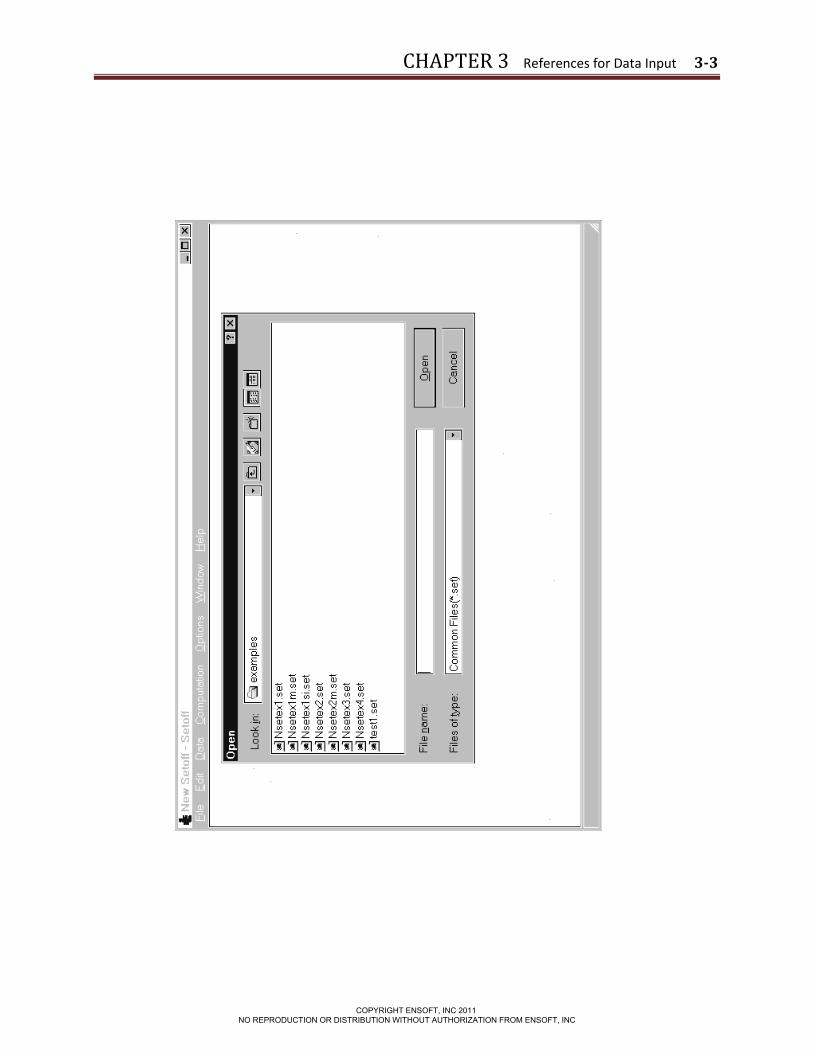
3.1.2 File - Open This is used to open a file that has been previously prepared and saved to disk. The File - Open window dialogis used to search for an existing input-data file. By default, the file is initially searched in the directory where SETOFF 3.0 was installed. Standard windows-navigation procedures may be used to locate the name and directory of the desired project file. This menu option may be accessed with the b+O keyboard combination.
Every analytical run of SETOFF 3.0 produces several additional files (as previously indicated in Table 2.1 of this manual). The name of the input-data file indicates the names of all related files produced by a successful execution (output and plot files). All the additional program files will be created in the same directory as the input file. Input-data files that are partially completed may be saved and later opened for completion, run, and view of results.
Opening some partially-completed SETOFF 3.0 input files or invalid data files may produce an information window reporting that an “invalid or incomplete” file is being opened. The user should click the OK button and all partial-input data that was previously prepared should become available.
3.1.3 File - Save This option is used to save input data under the current file name. With this method of storing data to disk, any input data that was previously saved with the same file name is replaced with the current parameters. Input-data files should be saved before proceeding with runs for analytical computation. This menu option may also be accessed with the b+S keyboard combination.
3.1.4 File - Save As This option allows the user to save any opened or new input-data file under a different file name or different directory. Any input-data file saved under an existing file name will replace the contents of the existing file.
3.1.5 File - Save Bitmap This option saves a screenshot of the 3D-View window as a bitmap.
3.1.6 File – Print This option prints the display in the 3D-View window.
COPYRIGHT ENSOFT, INC 2011 NO REPRODUCTION OR DISTRIBUTION WITHOUT AUTHORIZATION FROM ENSOFT, INC
CHAPTER 3 References for Data Input 3-3
COPYRIGHT ENSOFT, INC 2011 NO REPRODUCTION OR DISTRIBUTION WITHOUT AUTHORIZATION FROM ENSOFT, INC

CHAPTER 3 References for Data Input 3-4
3.1.7 File - Exit This is selected to exit SETOFF 3.0. Any input-data file that was modified and not yet saved to disk will produce a confirmation window before exiting the program (see Fig. 3.2).
3.2 Data Menu The input of specific parameters for an application is controlled under options contained within this menu (shown in Fig. 3.3). It is recommended that the user choose each submenu and enter parameters in a consecutive manner starting from the top option.
Selecting or clicking any of the submenu choices contained in the Data menu produces various types of windows. As a reminder of standard commands of Microsoft Windows®, open windows may be closed by all or some of the following methods:
• clicking the “OK” button (if available), or
• clicking the X box on the upper-right corner of the window, or
• double-clicking the SETOFF 3.0 icon on the upper-left corner of the window, or
• using the b+D keyboard combination, or
• clicking once on the SETOFF 3.0 icon on the upper-left corner of the window and then choosing Close.
Open Windows may optionally be left open on the screen. The selection of other menu options will then produce new windows on top of those that were left open.
Many sub-windows of the Data Menu will show an Add Row and/or Delete Row buttons. The Add Row button always adds new rows at the end after all existing rows. Clicking on the Delete Row button deletes the row where the cursor is located.
3.2.1 Numeric Data Entries Cells that require numeric data may accept entries of mathematical expressions in addition to simple numeric entries. Entering a mathematical expression works similarly to normal numeric data. The user types the expression that represents the data and presses the e key to calculate the entered expression and to display the numeric result in the same cell.
Table 3.1 below shows the list of supported operations and constants. The order of operations follows the order in the list of Table 3.1. Note that implicit multiplication (i.e. 2(4+6)) is not supported (instead, use 2*(4+6) for the previous example).
The two constants that are currently supported are PI and e. Implicit multiplications using constants is not supported (use 2*e instead of 2e). Negation of the constants PI or e is not allowed. For instance, instead of entering -PI the user must enter -(PI).
COPYRIGHT ENSOFT, INC 2011 NO REPRODUCTION OR DISTRIBUTION WITHOUT AUTHORIZATION FROM ENSOFT, INC

CHAPTER 3 References for Data Input 3-5
OPERATORS Symbol Description
() Parenthesis (may be nested) ^ Exponentiation * Multiplication / Division + Addition - Subtraction - Negation (same as subtraction)
CONSTANTS Symbol Value PI (or pi) 3.1415927 e (or E) 2.7182818
Table 3.1 Supported mathematical operations and constants
Scientific notation (i.e. 1 .65e8 or 1 .65e-8) may be used to input very large or very small numbers. After an expression is calculated, very large or very small numbers will be displayed using scientific notation.
3.2.2 System of Units The quantities used in program SETOFF v3.0 and the corresponding units are given in Table 3.2. Factors to make the internal conversions between English and SI systems are provided in Table 3.3. The English unit is multiplied by the pertinent factor to get the SI metric value. Conversely, the SI metric unit is divided by the factor to obtain the English unit.
3.2.3 Data - Title This option activates the window shown in Fig. 3.4, where the user can enter a line of text containing a general description for the application problem. Any combination of characters may be entered in the text box in order to describe a particular application. The user input will be restrained automatically once the maximum length of text is reached. This is done to prevent the user from going beyond the maximum permissible length of characters allowed for the title line.
Fig. 3.4 Window screen for sample Data – Title
COPYRIGHT ENSOFT, INC 2011 NO REPRODUCTION OR DISTRIBUTION WITHOUT AUTHORIZATION FROM ENSOFT, INC

CHAPTER 3 References for Data Input 3-6
3.2.4 Data - Soil Layer Data A sample of this window screen is shown in Fig. 3.5. In general, for the computation of settlement, the soil stratigraphy is initially used to divide the subsurface soils into a series of layers. These basic layers may have to be further divided so that a layer boundary is provided whenever any of the following occurs:
Fig. 3.5
(a) soil stratum boundary;
(b) groundwater level;
(c) change in effective unit weight;
(d) change in soil compressibility;
(e) depth for any foundation; and
(f) depth to any settlement point.
Particular care should be taken not to overlook item (e) and item (f) in the list above. The program will check for item (e) during data input and the run will terminate if the input depth for any foundation is not at an input-layer boundary. No such check, however, is made for item (f). If a settlement point is
COPYRIGHT ENSOFT, INC 2011 NO REPRODUCTION OR DISTRIBUTION WITHOUT AUTHORIZATION FROM ENSOFT, INC

CHAPTER 3 References for Data Input 3-7
located below the ground surface and not at a layer boundary, some error in the computed settlement may result. The magnitude of the error will depend on specific conditions and cannot be predicted. The entry will define the depth, effective unit weight, soil compressibility, and height factor for each soil strata. The number of soil layers is limited to 25.
This window entry will define the depth, effective unit weight, soil compressibility, and height factor for each soil strata. The maximum number of soil layers is limited to 25. General descriptions of the data needed in each column of the Soil Layer Data menu are the following:
• Soil Layer. This is a sequential number that is provided for each soil layer. This number is automatically provided by the program as new rows are added. The maximum number of rows of soil layers that may be used is limited to 25.
• Top Depth. This is the depth at the top of the soil layer being specified. The top of the first layer must always start at depth zero. Subsequent layers should start at the Bottom Depth of previous layers.
• Bottom Depth. This is the depth at the bottom of the soil layer being specified. The depth of the bottom of each layer should always be equal to the depth of the top of the immediately consecutive layer.
• Effective Unit Weight. Values of effective unit weight for each soil depth are entered in standard units of force per unit volume. Unit weight (mass density) is usually determined in the laboratory by direct measurements on undisturbed samples obtained from soil borings.
• Soil Compressibility Curve No. Users here specify the number (always an integer) of the compressibility curve that corresponds to each soil layer. Each curve number specified here is later defined under the menu Data - Soil Compressibility Curves.
• Soil Layer Thickness Factor, Hf. This is a number that may vary from 0 to 1.0, representing the relative portion of the soil-layer thickness to use in the settlement computation for that layer. Normally, this factor is 1.0. Suppose, however, that a soil layer is composed of alternating layers of clay and sand with the total layer thickness consisting of one-half clay and one-half sand. If compressibility data for the layer is based on a consolidation test on the clay portion, a computation using the full layer thickness would result in a computed settlement for this layer that would be too large. If a layer thickness factor of 0.5 is used, the computed settlement would be a better approximation for the layered soil.
3.2.5 Types of Compressibility Curves In program SETOFF, soil compressibility is entered using either data obtained from consolidation tests or taken as the slope of the linear compressibility curve. Three options are available for data input for soil compressibility. A sample window screen for this menu is shown on Fig. 3.6. After inputting the data, the soil compressibility curves can be applied to the corresponding soil layer in Data – Soil Layer Data.
COPYRIGHT ENSOFT, INC 2011 NO REPRODUCTION OR DISTRIBUTION WITHOUT AUTHORIZATION FROM ENSOFT, INC

CHAPTER 3 References for Data Input 3-8
Typically, the compressibility data are entered as curves of Percent Vertical Strain versus Applied Vertical Pressure. The applied vertical pressure is entered in kips/ft2 for English units and in kPa for SI metric units. Although the traditional method to present laboratory consolidation data has been to use Void Ratio, e, as the ordinate for the test curve, many laboratories now use Vertical Strain, frequently as a percent. For this program, vertical strain is entered as Percent Vertical Strain so that the input is in larger numbers. For example, a Percent Vertical Strain of 10.1, is a vertical strain pf 0.0101 in./in. or mm/mm. The input percent vertical strain is converted by the program internally to vertical strain for settlement computation. The simple relationship between Percent Vertical Strain, F, and Void Ratio, e, is as follows:
100)1()(
0
0 ×+−
=e
eeF (1)
where 0e = initial void ratio
Three options can be used to input the soil compressibility curves. ???Any input method can be used for any layer in any order or sequence???. However, only one option can be used per soil compressibility curve.
Option 1. The first input option is to define the semilog soil compressibility curve by a series of straight lines that best fit the curve. The curve to be input can be the actual laboratory test curve or one that has been modified by any method to produce a curve from the laboratory test results that is believed to better represent the actual field compressibility. The actual input are the coordinates, percent vertical strain and applied vertical pressure (on the log scale), of points that define the ends of the straight lines. A minimum of two points (one straight line) and a maximum of eight point (seven straight lines) must be used. The development of the data for input by Method 1 is illustrated on Fig. 3.7.
COPYRIGHT ENSOFT, INC 2011 NO REPRODUCTION OR DISTRIBUTION WITHOUT AUTHORIZATION FROM ENSOFT, INC

CHAPTER 3 References for Data Input 3-9
Fig. 3.7 Window screen for sample Data - Soil Compressibility Curves
Option 2. This option can be used where the semilog soil compressibility curve can be represented by a single straight line; this is a special case of Option 1 where there is only one line segment. The input is entered as the slope of the straight line and, for Option 2, is entered as a positive number, (+)CF. Examples of when this input method could be used are a normally-consolidated clay, a sand layer with small or zero compressibility, or an unloading, or rebounding, compressibility curve. The relationship between (+)CF and the coefficient of compressibility, Cc, (the slope of the semilog void ratio versus applied vertical pressure curve) is given by the following:
100)1(
)()(
0
×+
=+e
CCF C (2)
Option 3. The third option to enter soil compressibility is to enter the slope of an arithmetic Percent Vertical Strain versus Applied Vertical Pressure curve. To indicate that Method 3 is being used, ???the slope should be entered as a negative number???. This method is not used for routine settlement analyses. It has been used, for example, to develop influence values to use in iterative computations to obtain compatibility between computed soil consolidation settlement and computed structural deflections of large mat foundations. The slope to be input is related to the coefficient of volume compressibility, mv, and the coefficient of compressibility, av, in the Terzaghi Theory of Consolidation (Terzaghi 1943a) by the following:
100)( ×=− mvCF (3)
COPYRIGHT ENSOFT, INC 2011 NO REPRODUCTION OR DISTRIBUTION WITHOUT AUTHORIZATION FROM ENSOFT, INC
CHAPTER 3 References for Data Input 3-10
1001
)(0
×
+
=−e
aCF v (4)
3.2.6 Data - Soil Compressibility Curves A total of 10 different soil-compressibility curves can be specified on each SETOFF file. A general description for the data needed under each column for the submenu option Data – Soil Compressibility Curves is listed below.
• Curve No. This is a sequential number that is included for each soil compressibility curve. This number is automatically provided by the program as new rows are added. The maximum number of rows of soil-compressibility curves that may be used is limited to 10.
• Curve Description. Users may associate each compressibility curve with a textual description for each soil layer or for each consolidation test. Any letter or number may be used in this column.
• Option 1 - Data Points of Compressibility Curve. This button opens a new window where the user can input the points of the soil compressibility curve. As described in the previous section, this method defines a semilog soil compressibility curve by a series of straight lines that best fits the laboratory data from a consolidation test. The maximum number of points in each soil-compressibility curve is limited to 8 and the minimum limited to 2.
o The first column, % Change in Height, is the ordinate of points from the compressibility curve. They represent values of Percent Vertical Strain. For example, a Percent Vertical Strain of 10.1, represents a Vertical Strain of 0.0101 in./ in. or mm/mm. The values inputted for Percent Vertical Strain (% Change in Height) are internally converted by the program to Vertical Strain for the computations of settlement.
o The second column, Applied Vertical Pressure, represents the values of vertical pressure (in a log scale) applied during the consolidation test (usually in the horizontal axis).
• Option 2 – Slope of Semi-log Curves. The user can input the soil compressibility curve in this column as described as Option 2 in the previous section. The user must input a value computed from Equation 2 in Section 3.2.5. This is the standard consolidation curve where the vertical axis represents percent vertical strain (in arithmetic scale) and the horizontal axis represents applied vertical pressure (in logarithmic scale).
• Options 3 – Slope of Arithmetic Curves. The user can input the soil compressibility curve in this column as described as Option 3 in the previous section. The user must input a number with Equation 4 as shown in Section 3.2.5. This type of consolidation curve is not commonly used for routine settlement analysis. However, this method may be helpful to develop influence values used in iterative computations to obtain compatibility between computed soil consolidation settlement and computed structural deflections of large mat foundations. In these curves the vertical axis represents percent vertical strain (in arithmetic scale) and the horizontal axis represents applied vertical pressure (in arithmetic scale).
COPYRIGHT ENSOFT, INC 2011 NO REPRODUCTION OR DISTRIBUTION WITHOUT AUTHORIZATION FROM ENSOFT, INC

CHAPTER 3 References for Data Input 3-11
3.2.7 Data – Settlement Points Data The foundation plan consists of the arrangement of loaded areas comprising the foundation and the locations of the settlement points. The loaded areas may be footings, mats, and pile caps carrying structural loads or areas representing excavations that are not backfilled. A loaded area must be either rectangular or circular in shape. The loaded areas, however, may be entered in any order or combination desired.
The settlement points are the points where settlement is to be computed. They may be located anywhere in the foundation plan. They also may be located at or below the ground surface but, as indicated previously; they must be located on the surface of one of the soil layers established for the computation.
Locations of the loaded areas and the settlement points are defined by coordinates from a set of arbitrarily selected axes. The coordinates, however, must be positive; that is, the loaded areas and settlement points must be in the first quadrant of the coordinate system.
The location of each settlement point within the first quadrant of the established coordinate system is input by x-, and y-coordinate as shown in Fig. 3.9. Each point may be located at any depth provided it is located on the upper boundary of a soil layer established for the settlement computation. The soil layer number, on which the settlement point is located, is used to instruct the program at which the settlement computation begins. The maximum number of settlement points is limited to 25.
Fig. 3.9
COPYRIGHT ENSOFT, INC 2011 NO REPRODUCTION OR DISTRIBUTION WITHOUT AUTHORIZATION FROM ENSOFT, INC

CHAPTER 3 References for Data Input 3-12
3.2.8 Data – Foundation Configuration The number of shallow foundations (footings and mats) and deep foundations (pile foundations with pile caps) can be entered in the first two entries. A sample window is shown in Figure 3.10. The number of shallow and deep foundations that can be computed is limited to a combined total of 50.
The Pile-Capacity Options are used for pile foundations with pile caps. The option selected is applied to each pile foundation. The graphic on the right presents the details of each option:
• Friction piles with the fictitious footing located on the top of the friction zone-
• Friction piles with the fictitious footing located at the 1/3 depth of friction zone-
• End-bearing piles with the fictitious footing located at the top of the firm strata-
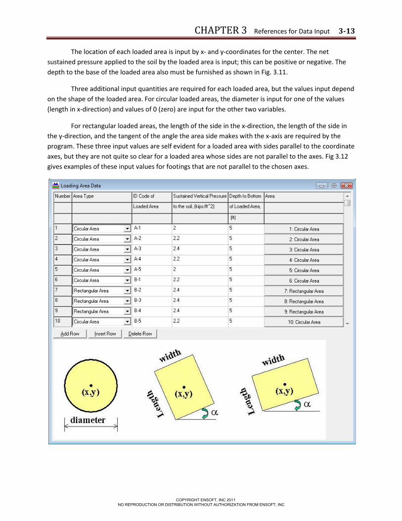
3.2.9 Data – Loaded Shallow Footings Area data Each shallow foundation loaded area is identified by a name with up to four alphanumeric characters. The shape of each loaded area is represented by an integer, 1 for rectangular or 2 for circular. ???The number of rows added should correspond to the number of shallow foundations entered in Data – Foundation Configuration.
COPYRIGHT ENSOFT, INC 2011 NO REPRODUCTION OR DISTRIBUTION WITHOUT AUTHORIZATION FROM ENSOFT, INC
CHAPTER 3 References for Data Input 3-13
The location of each loaded area is input by x- and y-coordinates for the center. The net sustained pressure applied to the soil by the loaded area is input; this can be positive or negative. The depth to the base of the loaded area also must be furnished as shown in Fig. 3.11.
Three additional input quantities are required for each loaded area, but the values input depend on the shape of the loaded area. For circular loaded areas, the diameter is input for one of the values (length in x-direction) and values of 0 (zero) are input for the other two variables.
For rectangular loaded areas, the length of the side in the x-direction, the length of the side in the y-direction, and the tangent of the angle the area side makes with the x-axis are required by the program. These three input values are self evident for a loaded area with sides parallel to the coordinate axes, but they are not quite so clear for a loaded area whose sides are not parallel to the axes. Fig 3.12 gives examples of these input values for footings that are not parallel to the chosen axes.
COPYRIGHT ENSOFT, INC 2011 NO REPRODUCTION OR DISTRIBUTION WITHOUT AUTHORIZATION FROM ENSOFT, INC

CHAPTER 3 References for Data Input 3-14
3.2.10 Data – Pile Foundation Data The coordinates and depth of the pile cap; dimensions of the pile group; area of zero friction and loading is entered in this window. A sample window is shown in Figure 3.xx. Each row corresponds to one deep foundation with a pile cap and pile group. The number of rows added should correspond to the number of pile foundations entered in Data – Foundation Configuration.
• X-Coord & Y-Coord at Center of Cap. Defines location of the center of pile foundation. It recommended to use only positive values for X and Y to avoid calculation errors in the program. The pile cap and pile group should avoid the negative regions of the XY plane.
• Length along X-direction. Defines the length of the pile group along the X direction.
• Length along Y-direction. Defines the length and width of the pile group along Y-direction. Areas in the negative region of the XY plane should be avoided. Check the X- and Y-coordinates
• Depth to the Base of the Pile Cap. Defines location of the bottom of the pile cap. This should be located at the surface of a soil layer.
• Depth of Zero Friction. Defines the zone of the zero friction zone. ???This value is taken from the top of the pile and then down along the length of the pile.
• Pile Length. Defines length of piles in pile group.
• Vertical Load at Pile Cap. Defines vertical load on the pile cap.
COPYRIGHT ENSOFT, INC 2011 NO REPRODUCTION OR DISTRIBUTION WITHOUT AUTHORIZATION FROM ENSOFT, INC

CHAPTER 4. References for Program Execution and Output Reviews
COPYRIGHT ENSOFT, INC 2011 NO REPRODUCTION OR DISTRIBUTION WITHOUT AUTHORIZATION FROM ENSOFT, INC

CHAPTER 4 References for Program Execution and Output Reviews 4-2
4.1 Introduction Chapter 4 presents options related to the execution of the program and includes methods of addressing run-time errors. This Chapter also includes suggestions for reviewing input, output, and processor text files. The final section of this Chapter includes descriptions of all the options that may be observed in graphical form. The commands covered in this chapter are contained in the top menu, under the Computation and the Graphics titles.
4.2 Computation Menu This menu option is selected to execute the program using the parameters that were saved in the input-data file. Other options contained under this menu are used to view the input data and output results. Detailed descriptions of the submenu options contained under the Computation menu are explained in the following topics.
4.2.1 Computation – Run Analysis An input file, after preparation or modification, must be saved to disk before selecting the Computation - Run Analysis, which executes the analytical module of program SETOFF 3.0. The module, a stand-alone program routine, is called for execution by the “shell” process of the environment in Microsoft Windows©
The user should remember to save the input data under a user-specified name before executing the analytical module. When saving data to disk, SETOFF 3.0 will automatically add an extension of the type *.set to the name of the input file.
A sub-window is usually produced during the execution of the module. When the module’s execution process is finished, the sub-window automatically disappears and the active command is returned to the Microsoft NotePad program which is used automatically to display the output in the text format.
At the beginning of the run, the analytical module will read the saved input data progressively. If an input-data format is incorrect during reading, the analytical module will stop immediately and in many cases it saves an error message and a status report in the output file. A detailed explanation of each error message is presented in Chapter 5. Once a successful run is produced, the user may proceed to the next items for observation of results.
4.2.2 Computation- Edit Input Text This submenu option is used to generate/edit the input-data file in plain-text mode as shown in Fig. 4.1. This command becomes active after new data files have been saved to disk or when opening existing data files. The command is helpful for experienced users who may just want to change one or two parameters quickly using the text editor, or for those users wishing to observe the prepared input data in text mode. A line-by-line description of the required-input data is included in Appendix of this manual.
This submenu automatically invokes the word processor or text editor specified in Options... under the Computation menu. The default setting uses the utility program named notepad. exe.
COPYRIGHT ENSOFT, INC 2011 NO REPRODUCTION OR DISTRIBUTION WITHOUT AUTHORIZATION FROM ENSOFT, INC

CHAPTER 4 References for Program Execution and Output Reviews 4-3
Input-data files are automatically saved to disk with the extension of *.set by program SETOFF 3.0. Use of the notepad for editing the input data for Example Problem 1 is shown in Fig. 4.3.
Fig. Input text
4.2.3 Computation- View Output Text This option displays the results of the analysis. The organization of results is displayed as a series of tables. The tables are listed as follows:
- Table 1: Problem Control Parameters - Table 2: Soil and Layer Information - Table 3: Soil Compressibility Source and Data
COPYRIGHT ENSOFT, INC 2011 NO REPRODUCTION OR DISTRIBUTION WITHOUT AUTHORIZATION FROM ENSOFT, INC

CHAPTER 4 References for Program Execution and Output Reviews 4-4
- Table 4: Settlement Point Data - Table 5: Loaded Area Information - Table 6: Average Stress Increase - Table 7: Computed Settlement
The default text editor is Microsoft NotePad. A sample output is shown in Fig. 4.4. Certain output files may be too large for the Microsoft Notepad editor, so other text editors may have to be used. (Microsoft WordPad should be able to open most text files.)
Fig. Output Text
4.3 View Menu This menu contains two options for displaying the settlement curve and 3-D model of the soil stratigraphy and foundations.
COPYRIGHT ENSOFT, INC 2011 NO REPRODUCTION OR DISTRIBUTION WITHOUT AUTHORIZATION FROM ENSOFT, INC

CHAPTER 4 References for Program Execution and Output Reviews 4-5
4.3.1 View – Graphics This option displays a plot of the computed settlement at selected settlement points. A graph will display a curve connecting the level of settlement at each settlement point.
4.3.2 View – 3D View This option displays a three dimensional model of the soil stratigraphy and foundations. A window of the 3D-View is shown in Fig. 4.5. This is a very useful view to check the locations and number of foundations and the soil stratigraphy. Selecting this option will enable a 3D viewing toolbar and the Show menu.
The 3D View toolbar allows you to manipulate the view of the soil and foundation model (Fig. 4.6). Placing the mouse cursor over the buttons will display the button’s function. A brief description of the toolbar is listed in the following:
4.4 Show Menu The Show menu provides various graphic options to view properties of the foundation plan in the 3D View window. Graphics screens contained under this menu are shown in Fig. 4.7. This menu is available only if the 3D View is selected in the View menu and as long as the 3D View window is open. The graphics options may be enabled or disabled for observation.
• Soil Layers: displays soil layers
• Soil Layer Labels: displays the label for each soil layer
• Soil Layer Depth Labels: displays the depth of each soil layer
• Footing Areas: displays footing areas representing shallow foundations
• Footing Areas Labels: displays ID Code of Loaded Area for footing foundations
• Pile Cap Blocks: displays pile cap blocks representing deep foundations
• Settlement Points: displays location of settlement points
• Settlement Results: opens Settlement Results window where graphical representation of output results can be displayed in 3D View. Here the user can select to show bar plots, values and points of settlement.
o Show Settlement Results: enables display for settlement results
COPYRIGHT ENSOFT, INC 2011 NO REPRODUCTION OR DISTRIBUTION WITHOUT AUTHORIZATION FROM ENSOFT, INC

CHAPTER 4 References for Program Execution and Output Reviews 4-6
o Show Bar Plot: displays a bar plot at each settlement point. This option is useful for comparing settlements at different points. The Bar Length and Width Factor can be adjusted to change the bar sizes for better viewing while maintaining the correct ratios for comparisons.
o Show Values: displays numerical values of settlement at each settlement point. The Only Maximums option displays only the maximum value.
o Show Settlement Points: same as Show – Settlement Points option
COPYRIGHT ENSOFT, INC 2011 NO REPRODUCTION OR DISTRIBUTION WITHOUT AUTHORIZATION FROM ENSOFT, INC
CHAPTER 5. Example Problems
COPYRIGHT ENSOFT, INC 2011 NO REPRODUCTION OR DISTRIBUTION WITHOUT AUTHORIZATION FROM ENSOFT, INC

CHAPTER 5 Example Problems 5-2
5.1 Introduction The output for the program SETOFF is presented in seven tables that are formatted to print on 8"”x1 1" sheets. Tables 1 and 2 are combined on one sheet and Tables 3-7 are “stand-alone” tables. A stand-alone table contains only one type of data and can be re-moved without materially affecting the continuity of the output. All of the output is considered important in verifying the input data and in aiding a manual check of the computed output. The user may elect, however, to remove and discard some of the output tables when retaining the computed results in a permanent job file.
5.2 Description of Output Tables The following paragraphs present brief descriptions of the information presented in the output tables
Table 1 - Units and Problem Parameters
This table shows the units selected for the settlement computation and the parameters that control the problem. These parameters include the number of soil layers, number of soil compressibilities, number of settlement points and number of loaded areas that define the scope of the computation.
Table 2 - Soil and Layer Information
This table is combined with Table 1 on the first sheet of the printout. The information in the table consists of input data and values computed from the input data. The input data presented are the soil layer number, the thickness factor for the layer, the effective unit weight of the soil in the layer, and the number of the soil compressibility for the layer. The computed values include the depth to the center of the layer, the thickness of the layer, the overburden pressure at the center of the layer, and the initial percent vertical strain for the soil in the layer.
Table 3 - Soil Compressibility Data
This is a stand-alone table and it can have up to 2 sheets with up to 7 soil compressibilities per sheet. The information presented for each soil compressibility is the compressibility number, a description and source for the soil compressibility, and the soil compressibility. For a semilog nonlinear curve, the soil compressibility data consists of a series of percent vertical strain and applied vertical pressure values representing points defining the nonlinear compressibility curve. For a linear curve, the soil compressibility data is the slope of the curve, a positive value for a semilog curve or a negative value for an arithmetic curve.
Table 4 - Settlement Point Data
This is a stand-alone table and it will consist of 1 sheet. The data presented for each settlement point are the x- and y-coordinate for the point and the number of the soil layer on which it is located.
Table 5 - Loaded Area Data
This is a stand-alone table and it can consist of up to 2 sheets with up to 36 loaded areas per sheet. The data for each loaded area consists of: an identification for the area; an indication of the shape (1 for
COPYRIGHT ENSOFT, INC 2011 NO REPRODUCTION OR DISTRIBUTION WITHOUT AUTHORIZATION FROM ENSOFT, INC
CHAPTER 5 Example Problems 5-3
rectangle or 2 for circle); the x- and y- coordinate for the center of the loaded area; the length in the x-direction, the length in the y-direction, and the slope with the x-axis for rectangular areas (diameter, zero and zero for circular areas); the sustained pressure applied to the soil by the area; and the depth to the base of the area.
Table 6 - Average Stress Increase
The is a stand-alone table, and it probable is the least important table to retain permanently. The information presented is the computed average stress increase at the center of each layer beneath each settlement point. The table can have 1 to 8 sheets with data for up to 7 settlement points and up to 18 layers on each sheet.
Table 7 - Computed Settlement
This is a stand-alone table, and it presents the computed settlements which are the primary reason for the use of the program SETOFF. The information presented is the computed settlement for each soil layer beneath each settlement point with a total settlement for each settlement point. The table can have 1 to 8 sheets with up to 7 settlement points and up to 18 layers on each sheet.
The computed settlement for each layer and the total settlement for each settlement point is presented so the user can make his own analysis of the settlement. The computer, being an unreasoning machine, can compute and total many small settlements that may not actually occur in the field. Many years ago Terzaghi (1941) advanced a hypothesis that consolidation of undisturbed clay does not occur unless the stress increase exceeds some “threshold” value. A rule-of-thumb for this “threshold” value is a stress increase of about ten percent of the effective overburden pressure. The user may elect to use a smaller number of layers for the settlement by manually totaling the computed settlements for this smaller number of layers. For consistency, however, the same number of layers should be used for all settlement points,
5.3 Example 1 The input and output for Example Problem 1 are presented in the following pages. The soil conditions for this example problem are shown in Fig. 5-1 with one of the soil compressibility curves shown in Fig. 5-2. The foundation and settlement plan for the example are shown in Fig. 5-3.
COPYRIGHT ENSOFT, INC 2011 NO REPRODUCTION OR DISTRIBUTION WITHOUT AUTHORIZATION FROM ENSOFT, INC

CHAPTER 5 Example Problems 5-4
Fig. 5.1 Soil conditions for Example Problem 1
COPYRIGHT ENSOFT, INC 2011 NO REPRODUCTION OR DISTRIBUTION WITHOUT AUTHORIZATION FROM ENSOFT, INC

CHAPTER 5 Example Problems 5-5
Fig. 5.2 Soil Compressibility curve for Example Problem 1
COPYRIGHT ENSOFT, INC 2011 NO REPRODUCTION OR DISTRIBUTION WITHOUT AUTHORIZATION FROM ENSOFT, INC

CHAPTER 5 Example Problems 5-6
Fig. 5.3 Foundation plan for Example Problem 1
COPYRIGHT ENSOFT, INC 2011 NO REPRODUCTION OR DISTRIBUTION WITHOUT AUTHORIZATION FROM ENSOFT, INC

CHAPTER 5 Example Problems 5-7
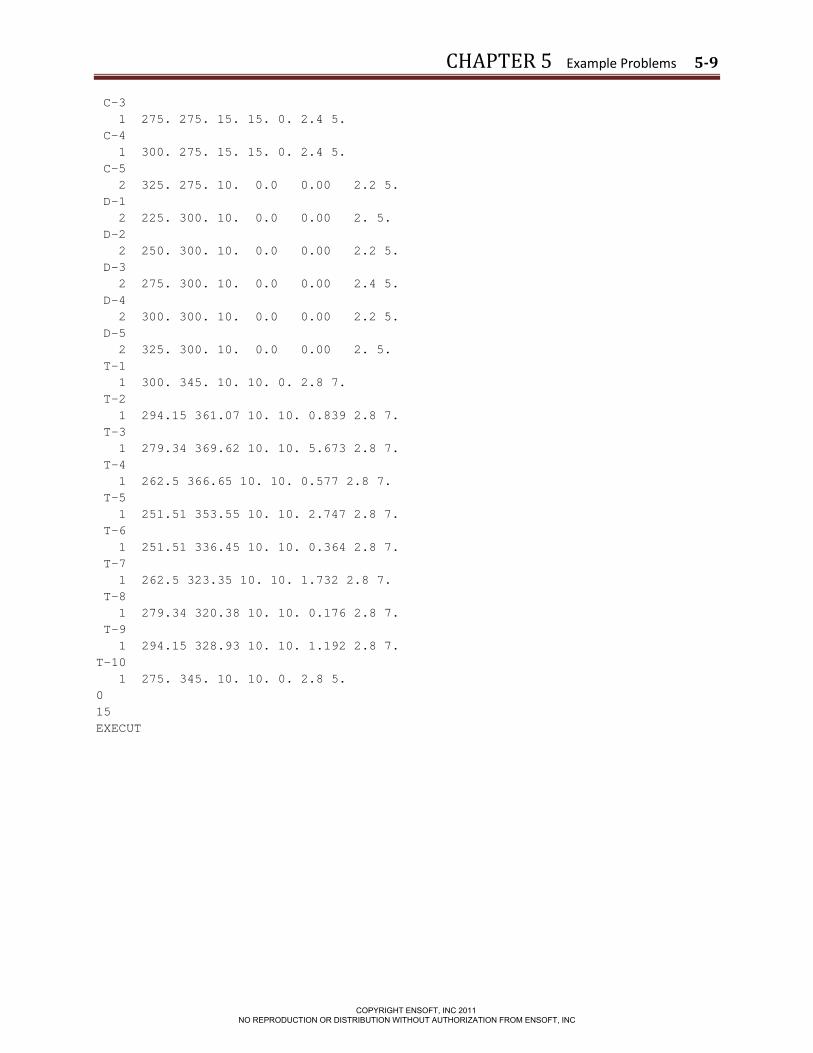
5.3.1 Input Data SETOFF Version 3.01 SETOFF EXAMPLE PROBLEM A - CWF - APRIL 24, 1990 1 17 6 13 30 1 5. 122. 1 1. 2 7. 122. 1 1. 3 9. 122. 1 1. 4 12. 120. 1 1. 5 15. 120. 1 1. 6 18. 58. 1 1. 7 21. 66. 2 1. 8 24. 68. 2 1. 9 28. 68. 2 1. 10 32. 70. 2 1. 11 37. 70. 3 1. 12 47. 70. 4 1. 13 57. 70. 4 1. 14 67. 68. 5 1. 15 77. 68. 5 1. 16 87. 64. 6 1. 17 100. 64. 6 1. 1 7 CONSOLIDATION TEST 70-053, BORING 2, 15 FT (MODIFIED) 0. 0.5 1.1 3. 1.5 4. 1.9 5. 2.65 6. 4.5 8. 13. 32. 2 7 CONSOLIDATION TEST 70-053, BORING 2, 35 FT (MODIFIED) 0. 0.7 0.7 3. 1. 4. 1.5 5. 2.1 6. 3.2 8. 9.5 32. 3 1 SAND LAYER, ASSUMED INCOMPRESSIBLE 0.001 4 5 CONSOLIDATION TEST 70-053, BORING 4, 50 FT 0. 1.88 0.6 4. 1.62 8. 2.85 16. 4.7 32. 5 5
COPYRIGHT ENSOFT, INC 2011 NO REPRODUCTION OR DISTRIBUTION WITHOUT AUTHORIZATION FROM ENSOFT, INC

CHAPTER 5 Example Problems 5-8
CONSOLIDATION TEST 70-053, BORING 2, 65 FT 0. 1.86 1.16 4. 2.64 8. 4.22 16. 6.36 32. 6 7 CONSOLIDATION TEST 70-053, BORING 4, 90 FT 0. 1.46 0.2 2. 1.06 4. 3.4 8. 4.1 16. 4.9 20. 7.2 32. 1 225. 225. 2 2 225. 250. 2 3 225. 275. 2 4 250. 275. 2 5 275. 275. 2 6 275. 300. 2 7 250. 300. 2 8 225. 300. 2 9 279.34 369.62 2 10 275. 345. 2 11 262.5 323.35 2 12 279.34 320.38 2 13 300. 300. 2 A-1 2 225. 225. 10. 0.0 0.00 2. 5. A-2 2 250. 225. 10. 0.0 0.00 2.2 5. A-3 2 275. 225. 10. 0.0 0.00 2.4 5. A-4 2 300. 225. 10. 0.0 0.00 2.2 5. A-5 2 325. 225. 10. 0.0 0.00 2. 5. B-1 2 225. 250. 10. 0.0 0.00 2.2 5. B-2 1 250. 250. 15. 15. 0. 2.4 5. B-3 1 275. 250. 15. 15. 0. 2.4 5. B-4 1 300. 250. 15. 15. 0. 2.4 5. B-5 2 325. 250. 10. 0.0 0.00 2.2 5. C-1 2 225. 275. 10. 0.0 0.00 2.2 5. C-2 1 250. 275. 15. 15. 0. 2.4 5.
COPYRIGHT ENSOFT, INC 2011 NO REPRODUCTION OR DISTRIBUTION WITHOUT AUTHORIZATION FROM ENSOFT, INC
CHAPTER 5 Example Problems 5-9
C-3 1 275. 275. 15. 15. 0. 2.4 5. C-4 1 300. 275. 15. 15. 0. 2.4 5. C-5 2 325. 275. 10. 0.0 0.00 2.2 5. D-1 2 225. 300. 10. 0.0 0.00 2. 5. D-2 2 250. 300. 10. 0.0 0.00 2.2 5. D-3 2 275. 300. 10. 0.0 0.00 2.4 5. D-4 2 300. 300. 10. 0.0 0.00 2.2 5. D-5 2 325. 300. 10. 0.0 0.00 2. 5. T-1 1 300. 345. 10. 10. 0. 2.8 7. T-2 1 294.15 361.07 10. 10. 0.839 2.8 7. T-3 1 279.34 369.62 10. 10. 5.673 2.8 7. T-4 1 262.5 366.65 10. 10. 0.577 2.8 7. T-5 1 251.51 353.55 10. 10. 2.747 2.8 7. T-6 1 251.51 336.45 10. 10. 0.364 2.8 7. T-7 1 262.5 323.35 10. 10. 1.732 2.8 7. T-8 1 279.34 320.38 10. 10. 0.176 2.8 7. T-9 1 294.15 328.93 10. 10. 1.192 2.8 7. T-10 1 275. 345. 10. 10. 0. 2.8 5. 0 15 EXECUT
COPYRIGHT ENSOFT, INC 2011 NO REPRODUCTION OR DISTRIBUTION WITHOUT AUTHORIZATION FROM ENSOFT, INC

CHAPTER 5 Example Problems 5-10
5.3.2 Output Results
******************************************
* * * FOUNDATION SETTLEMENT ANALYSIS * * * ****************************************** SETOFF Version 3.01 SETOFF EXAMPLE PROBLEM A - CWF - APRIL 24, 1990 TABLE 1 - PROBLEM CONTROL PARAMETERS COMPUTATION UNITS = 1 1 = U.S. GRAVITATIONAL SYSTEM 2 = S.I. ABSOLUTE SYSTEM NUMBER OF SOIL LAYERS = 17 NUMBER OF SOIL COMPRESSIBILITIES = 6 NUMBER OF SETTLEMENT POINTS = 13 NUMBER OF LOADED AREAS = 30 TABLE 2 - SOIL AND LAYER INFORMATION SOIL DEPTH TO LAYER LAYER UNIT SOIL OVERBURDEN INIT VERTICAL LAYER CENTER THICKNESS THICK. WEIGHT COMP PRESSURE STRAIN (F0) NO. FT FT FACTOR LB/FT**3 NO. KSF % 1 2.50 5.00 1.00 122.00 1 0.305 0.000 2 6.00 2.00 1.00 122.00 1 0.732 0.234 3 8.00 2.00 1.00 122.00 1 0.976 0.411 4 10.50 3.00 1.00 120.00 1 1.278 0.576 5 13.50 3.00 1.00 120.00 1 1.638 0.728 6 16.50 3.00 1.00 58.00 1 1.905 0.821 7 19.50 3.00 1.00 66.00 2 2.091 0.526 8 22.50 3.00 1.00 68.00 2 2.292 0.571 9 26.00 4.00 1.00 68.00 2 2.530 0.618 10 30.00 4.00 1.00 70.00 2 2.806 0.668 11 34.50 5.00 1.00 70.00 3 3.121 0.000 12 42.00 10.00 1.00 70.00 4 3.646 0.526 13 52.00 10.00 1.00 70.00 4 4.346 0.722 14 62.00 10.00 1.00 68.00 5 5.036 1.652 15 72.00 10.00 1.00 68.00 5 5.716 1.922 16 82.00 10.00 1.00 64.00 6 6.376 2.634 17 93.50 13.00 1.00 64.00 6 7.112 3.003
COPYRIGHT ENSOFT, INC 2011 NO REPRODUCTION OR DISTRIBUTION WITHOUT AUTHORIZATION FROM ENSOFT, INC

CHAPTER 5 Example Problems 5-11
****************************************** * * * FOUNDATION SETTLEMENT ANALYSIS * * * ****************************************** SETOFF Version 3.01 SETOFF EXAMPLE PROBLEM A - CWF - APRIL 24, 1990 TABLE 3 - SOIL COMPRESSIBILITY SOURCE AND DATA SOIL COMPRESSIBILITY NO. 1 CONSOLIDATION TEST 70-053, BORING 2, 15 FT (MODIFIED) F P (%) 0.000 0.500 0.011 3.000 0.015 4.000 0.019 5.000 0.026 6.000 0.045 8.000 0.130 32.000 SOIL COMPRESSIBILITY NO. 2 CONSOLIDATION TEST 70-053, BORING 2, 35 FT (MODIFIED) F P (%) 0.000 0.700 0.007 3.000 0.010 4.000 0.015 5.000 0.021 6.000 0.032 8.000 0.095 32.000 SOIL COMPRESSIBILITY NO. 3 SAND LAYER, ASSUMED INCOMPRESSIBLE THE SLOPE OF THE F(%)-LOG P CURVE IS 0.001 SOIL COMPRESSIBILITY NO. 4 CONSOLIDATION TEST 70-053, BORING 4, 50 FT
COPYRIGHT ENSOFT, INC 2011 NO REPRODUCTION OR DISTRIBUTION WITHOUT AUTHORIZATION FROM ENSOFT, INC

CHAPTER 5 Example Problems 5-12
F P (%) 0.000 1.880 0.006 4.000 0.016 8.000 0.028 16.000 0.047 32.000 SOIL COMPRESSIBILITY NO. 5 CONSOLIDATION TEST 70-053, BORING 2, 65 FT F P (%) 0.000 1.860 0.012 4.000 0.026 8.000 0.042 16.000 0.064 32.000 SOIL COMPRESSIBILITY NO. 6 CONSOLIDATION TEST 70-053, BORING 4, 90 FT F P (%) 0.000 1.460 0.002 2.000 0.011 4.000 0.034 8.000 0.041 16.000 0.049 20.000 0.072 32.000
COPYRIGHT ENSOFT, INC 2011 NO REPRODUCTION OR DISTRIBUTION WITHOUT AUTHORIZATION FROM ENSOFT, INC

CHAPTER 5 Example Problems 5-13
****************************************** * * * FOUNDATION SETTLEMENT ANALYSIS * * * ****************************************** SETOFF Version 3.01 SETOFF EXAMPLE PROBLEM A - CWF - APRIL 24, 1990 TABLE 4 - SETTLEMENT POINT DATA POINT POINT COORDINATES LAYER NO, X Y NO.* FT FT 1 225.00 225.00 2 2 225.00 250.00 2 3 225.00 275.00 2 4 250.00 275.00 2 5 275.00 275.00 2 6 275.00 300.00 2 7 250.00 300.00 2 8 225.00 300.00 2 9 279.34 369.62 2 10 275.00 345.00 2 11 262.50 323.35 2 12 279.34 320.38 2 13 300.00 300.00 2 * NUMBER OF SOIL LAYER AT WHICH SETTLEMENT COMPUTATION BEGINS
COPYRIGHT ENSOFT, INC 2011 NO REPRODUCTION OR DISTRIBUTION WITHOUT AUTHORIZATION FROM ENSOFT, INC
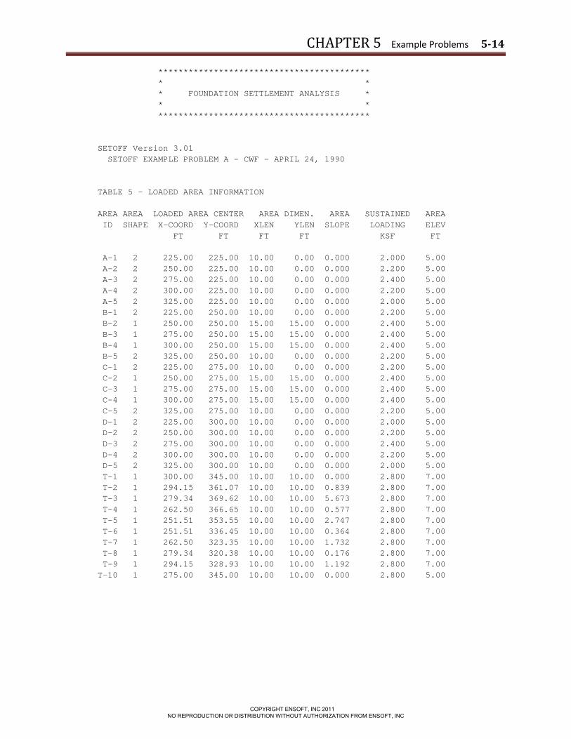
CHAPTER 5 Example Problems 5-14
****************************************** * * * FOUNDATION SETTLEMENT ANALYSIS * * * ****************************************** SETOFF Version 3.01 SETOFF EXAMPLE PROBLEM A - CWF - APRIL 24, 1990 TABLE 5 - LOADED AREA INFORMATION AREA AREA LOADED AREA CENTER AREA DIMEN. AREA SUSTAINED AREA ID SHAPE X-COORD Y-COORD XLEN YLEN SLOPE LOADING ELEV FT FT FT FT KSF FT A-1 2 225.00 225.00 10.00 0.00 0.000 2.000 5.00 A-2 2 250.00 225.00 10.00 0.00 0.000 2.200 5.00 A-3 2 275.00 225.00 10.00 0.00 0.000 2.400 5.00 A-4 2 300.00 225.00 10.00 0.00 0.000 2.200 5.00 A-5 2 325.00 225.00 10.00 0.00 0.000 2.000 5.00 B-1 2 225.00 250.00 10.00 0.00 0.000 2.200 5.00 B-2 1 250.00 250.00 15.00 15.00 0.000 2.400 5.00 B-3 1 275.00 250.00 15.00 15.00 0.000 2.400 5.00 B-4 1 300.00 250.00 15.00 15.00 0.000 2.400 5.00 B-5 2 325.00 250.00 10.00 0.00 0.000 2.200 5.00 C-1 2 225.00 275.00 10.00 0.00 0.000 2.200 5.00 C-2 1 250.00 275.00 15.00 15.00 0.000 2.400 5.00 C-3 1 275.00 275.00 15.00 15.00 0.000 2.400 5.00 C-4 1 300.00 275.00 15.00 15.00 0.000 2.400 5.00 C-5 2 325.00 275.00 10.00 0.00 0.000 2.200 5.00 D-1 2 225.00 300.00 10.00 0.00 0.000 2.000 5.00 D-2 2 250.00 300.00 10.00 0.00 0.000 2.200 5.00 D-3 2 275.00 300.00 10.00 0.00 0.000 2.400 5.00 D-4 2 300.00 300.00 10.00 0.00 0.000 2.200 5.00 D-5 2 325.00 300.00 10.00 0.00 0.000 2.000 5.00 T-1 1 300.00 345.00 10.00 10.00 0.000 2.800 7.00 T-2 1 294.15 361.07 10.00 10.00 0.839 2.800 7.00 T-3 1 279.34 369.62 10.00 10.00 5.673 2.800 7.00 T-4 1 262.50 366.65 10.00 10.00 0.577 2.800 7.00 T-5 1 251.51 353.55 10.00 10.00 2.747 2.800 7.00 T-6 1 251.51 336.45 10.00 10.00 0.364 2.800 7.00 T-7 1 262.50 323.35 10.00 10.00 1.732 2.800 7.00 T-8 1 279.34 320.38 10.00 10.00 0.176 2.800 7.00 T-9 1 294.15 328.93 10.00 10.00 1.192 2.800 7.00 T-10 1 275.00 345.00 10.00 10.00 0.000 2.800 5.00
COPYRIGHT ENSOFT, INC 2011 NO REPRODUCTION OR DISTRIBUTION WITHOUT AUTHORIZATION FROM ENSOFT, INC
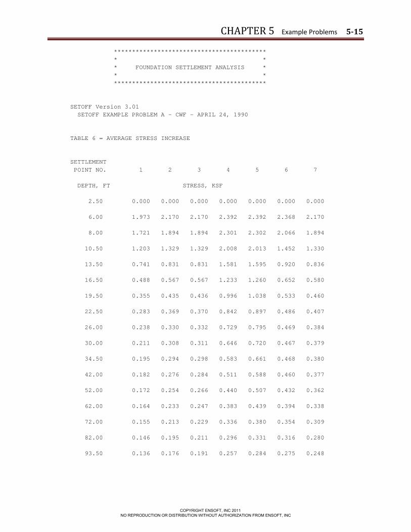
CHAPTER 5 Example Problems 5-15
****************************************** * * * FOUNDATION SETTLEMENT ANALYSIS * * * ****************************************** SETOFF Version 3.01 SETOFF EXAMPLE PROBLEM A - CWF - APRIL 24, 1990 TABLE 6 = AVERAGE STRESS INCREASE SETTLEMENT POINT NO. 1 2 3 4 5 6 7 DEPTH, FT STRESS, KSF 2.50 0.000 0.000 0.000 0.000 0.000 0.000 0.000 6.00 1.973 2.170 2.170 2.392 2.392 2.368 2.170 8.00 1.721 1.894 1.894 2.301 2.302 2.066 1.894 10.50 1.203 1.329 1.329 2.008 2.013 1.452 1.330 13.50 0.741 0.831 0.831 1.581 1.595 0.920 0.836 16.50 0.488 0.567 0.567 1.233 1.260 0.652 0.580 19.50 0.355 0.435 0.436 0.996 1.038 0.533 0.460 22.50 0.283 0.369 0.370 0.842 0.897 0.486 0.407 26.00 0.238 0.330 0.332 0.729 0.795 0.469 0.384 30.00 0.211 0.308 0.311 0.646 0.720 0.467 0.379 34.50 0.195 0.294 0.298 0.583 0.661 0.468 0.380 42.00 0.182 0.276 0.284 0.511 0.588 0.460 0.377 52.00 0.172 0.254 0.266 0.440 0.507 0.432 0.362 62.00 0.164 0.233 0.247 0.383 0.439 0.394 0.338 72.00 0.155 0.213 0.229 0.336 0.380 0.354 0.309 82.00 0.146 0.195 0.211 0.296 0.331 0.316 0.280 93.50 0.136 0.176 0.191 0.257 0.284 0.275 0.248
COPYRIGHT ENSOFT, INC 2011 NO REPRODUCTION OR DISTRIBUTION WITHOUT AUTHORIZATION FROM ENSOFT, INC

CHAPTER 5 Example Problems 5-16
****************************************** * * * FOUNDATION SETTLEMENT ANALYSIS * * * ****************************************** SETOFF Version 3.01 SETOFF EXAMPLE PROBLEM A - CWF - APRIL 24, 1990 TABLE 6 = AVERAGE STRESS INCREASE (CONT) SETTLEMENT POINT NO. 8 9 10 11 12 13 DEPTH, FT STRESS, KSF 2.50 0.000 0.000 0.000 0.000 0.000 0.000 6.00 1.973 0.467 2.771 0.467 0.467 2.170 8.00 1.721 2.772 2.486 2.772 2.773 1.894 10.50 1.203 2.371 1.842 2.374 2.377 1.330 13.50 0.741 1.644 1.214 1.653 1.660 0.836 16.50 0.490 1.138 0.861 1.156 1.168 0.580 19.50 0.359 0.855 0.689 0.886 0.902 0.459 22.50 0.289 0.695 0.611 0.738 0.758 0.406 26.00 0.249 0.584 0.572 0.641 0.663 0.384 30.00 0.227 0.501 0.550 0.573 0.596 0.378 34.50 0.218 0.438 0.528 0.523 0.545 0.379 42.00 0.216 0.366 0.480 0.465 0.486 0.377 52.00 0.216 0.299 0.411 0.406 0.426 0.362 62.00 0.214 0.252 0.348 0.358 0.375 0.338 72.00 0.206 0.218 0.298 0.317 0.332 0.309 82.00 0.196 0.191 0.258 0.282 0.293 0.280 93.50 0.183 0.167 0.221 0.246 0.256 0.248
COPYRIGHT ENSOFT, INC 2011 NO REPRODUCTION OR DISTRIBUTION WITHOUT AUTHORIZATION FROM ENSOFT, INC
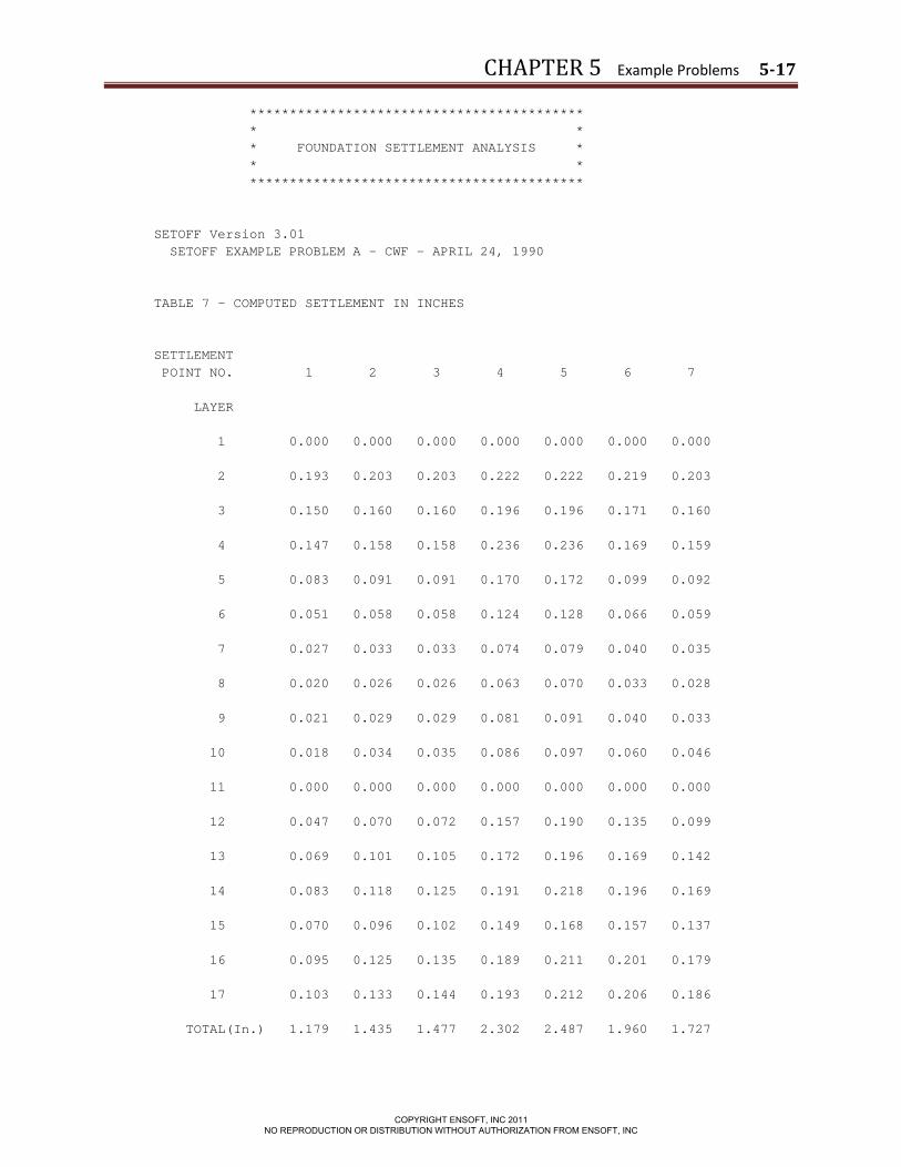
CHAPTER 5 Example Problems 5-17
****************************************** * * * FOUNDATION SETTLEMENT ANALYSIS * * * ****************************************** SETOFF Version 3.01 SETOFF EXAMPLE PROBLEM A - CWF - APRIL 24, 1990 TABLE 7 - COMPUTED SETTLEMENT IN INCHES SETTLEMENT POINT NO. 1 2 3 4 5 6 7 LAYER 1 0.000 0.000 0.000 0.000 0.000 0.000 0.000 2 0.193 0.203 0.203 0.222 0.222 0.219 0.203 3 0.150 0.160 0.160 0.196 0.196 0.171 0.160 4 0.147 0.158 0.158 0.236 0.236 0.169 0.159 5 0.083 0.091 0.091 0.170 0.172 0.099 0.092 6 0.051 0.058 0.058 0.124 0.128 0.066 0.059 7 0.027 0.033 0.033 0.074 0.079 0.040 0.035 8 0.020 0.026 0.026 0.063 0.070 0.033 0.028 9 0.021 0.029 0.029 0.081 0.091 0.040 0.033 10 0.018 0.034 0.035 0.086 0.097 0.060 0.046 11 0.000 0.000 0.000 0.000 0.000 0.000 0.000 12 0.047 0.070 0.072 0.157 0.190 0.135 0.099 13 0.069 0.101 0.105 0.172 0.196 0.169 0.142 14 0.083 0.118 0.125 0.191 0.218 0.196 0.169 15 0.070 0.096 0.102 0.149 0.168 0.157 0.137 16 0.095 0.125 0.135 0.189 0.211 0.201 0.179 17 0.103 0.133 0.144 0.193 0.212 0.206 0.186 TOTAL(In.) 1.179 1.435 1.477 2.302 2.487 1.960 1.727
COPYRIGHT ENSOFT, INC 2011 NO REPRODUCTION OR DISTRIBUTION WITHOUT AUTHORIZATION FROM ENSOFT, INC

CHAPTER 5 Example Problems 5-18
****************************************** * * * FOUNDATION SETTLEMENT ANALYSIS * * * ****************************************** SETOFF Version 3.01 SETOFF EXAMPLE PROBLEM A - CWF - APRIL 24, 1990 TABLE 7 - COMPUTED SETTLEMENT IN INCHES (CONT) SETTLEMENT POINT NO. 8 9 10 11 12 13 LAYER 1 0.000 0.000 0.000 0.000 0.000 0.000 2 0.193 0.073 0.260 0.073 0.073 0.203 3 0.150 0.241 0.214 0.241 0.241 0.160 4 0.147 0.288 0.209 0.289 0.289 0.159 5 0.083 0.180 0.123 0.181 0.183 0.092 6 0.051 0.108 0.083 0.111 0.113 0.059 7 0.028 0.060 0.050 0.061 0.062 0.035 8 0.021 0.046 0.041 0.051 0.053 0.028 9 0.022 0.058 0.056 0.068 0.071 0.033 10 0.021 0.065 0.072 0.076 0.079 0.046 11 0.000 0.000 0.000 0.000 0.000 0.000 12 0.055 0.094 0.144 0.137 0.147 0.099 13 0.086 0.118 0.161 0.159 0.166 0.142 14 0.108 0.127 0.174 0.179 0.187 0.169 15 0.093 0.098 0.133 0.141 0.147 0.137 16 0.126 0.123 0.165 0.180 0.187 0.179 17 0.138 0.126 0.166 0.185 0.192 0.186 TOTAL(In.) 1.322 1.805 2.052 2.131 2.190 1.726
COPYRIGHT ENSOFT, INC 2011 NO REPRODUCTION OR DISTRIBUTION WITHOUT AUTHORIZATION FROM ENSOFT, INC

CHAPTER 5 Example Problems 5-19
5.4 Example 2 The following example deals with settlement on a single deep foundation. The soil conditions and foundation parameters for this example problem are shown in Fig. 5.4. A guide through data input, analysis execution, and result review will be described in the following.
5.4.1 Problem Description A pile group 2.75m by 2.75m is placed in a deep clay stratum supporting a vertical load of 1335kN. The soil stratigraphy consists of a 6m sand layer and a 26m clay layer reaching bedrock. The soil stratum is divided into 5 layers with the respective properties of unit weight and soil compressibility. The unit weights and compressibilities of the soil is shown in Fig. 5.4. The sand can be assumed to be incompressible and the clay is provided with the void ratio and coefficient of compressibility.
COPYRIGHT ENSOFT, INC 2011 NO REPRODUCTION OR DISTRIBUTION WITHOUT AUTHORIZATION FROM ENSOFT, INC

CHAPTER 5 Example Problems 5-20
5.4.2 Data Input
5.4.2.1 Options – Units Before proceeding to data input it is a good idea to select the type of units you will be working with. By default, standardized units are set to English Units. For this example, information is provided in SI units so SI Units will be selected under the Options menu.
5.4.2.2 Data – Title Go to Data – Title to enter a description for the project.
5.4.2.3 Data – Soil Layer Data Go to Data – Soil Layer Data to define the soil layers.
COPYRIGHT ENSOFT, INC 2011 NO REPRODUCTION OR DISTRIBUTION WITHOUT AUTHORIZATION FROM ENSOFT, INC

CHAPTER 5 Example Problems 5-21
More rows can be added with the “Add Row” button or “A” hotkey to define the 5 layers. In the first column, enter the depths of the top of each layer. The first layer must be set to 0m at the top depth. Enter the depth to the bottom of the layer in the 2nd column. Note for the third column the value is only for the effective unit weight. For layers 2-5 the unit weight of water is subtracted from the saturated unit weight to obtain the effective unit weights. The soil compressibilities are defined in the next option Data – Soil Compressibilities. For now it is simply enumerated. Finally the layer thickness factor can be set to 1.
5.4.2.4 Data Soil Compressibility Data Go to Data – Soil Compressibility Data
The 1st column for identification has been set to the same values entered in Data – Soil Layer Data for convenience. Option 2 will be used for this case since the compressibility data shown in Fig. 5.4 is provided as coefficients of compressibility with a void ratio.
COPYRIGHT ENSOFT, INC 2011 NO REPRODUCTION OR DISTRIBUTION WITHOUT AUTHORIZATION FROM ENSOFT, INC
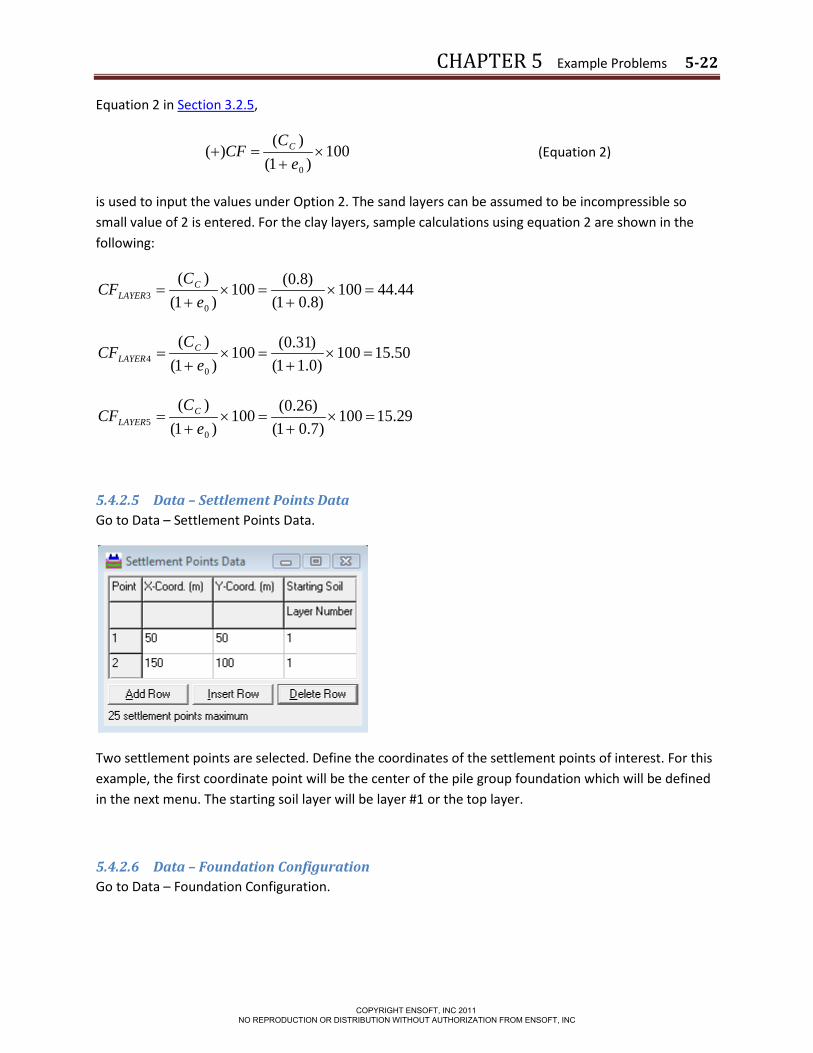
CHAPTER 5 Example Problems 5-22
Equation 2 in Section 3.2.5,
100)1(
)()(
0
×+
=+e
CCF C (Equation 2)
is used to input the values under Option 2. The sand layers can be assumed to be incompressible so small value of 2 is entered. For the clay layers, sample calculations using equation 2 are shown in the following:
44.44100)8.01(
)8.0(100)1(
)(
03 =×
+=×
+=
eC
CF CLAYER
50.15100)0.11(
)31.0(100)1(
)(
04 =×
+=×
+=
eC
CF CLAYER
29.15100)7.01(
)26.0(100)1(
)(
05 =×
+=×
+=
eC
CF CLAYER
5.4.2.5 Data – Settlement Points Data Go to Data – Settlement Points Data.
Two settlement points are selected. Define the coordinates of the settlement points of interest. For this example, the first coordinate point will be the center of the pile group foundation which will be defined in the next menu. The starting soil layer will be layer #1 or the top layer.
5.4.2.6 Data – Foundation Configuration Go to Data – Foundation Configuration.
COPYRIGHT ENSOFT, INC 2011 NO REPRODUCTION OR DISTRIBUTION WITHOUT AUTHORIZATION FROM ENSOFT, INC
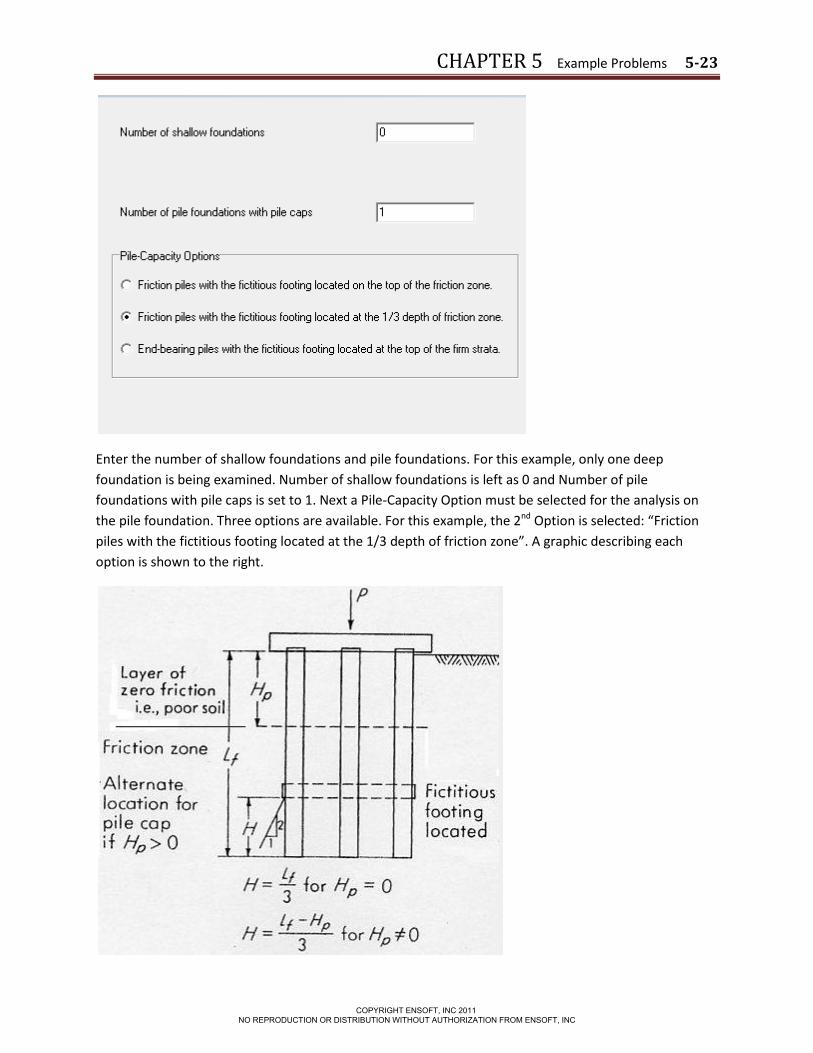
CHAPTER 5 Example Problems 5-23
Enter the number of shallow foundations and pile foundations. For this example, only one deep foundation is being examined. Number of shallow foundations is left as 0 and Number of pile foundations with pile caps is set to 1. Next a Pile-Capacity Option must be selected for the analysis on the pile foundation. Three options are available. For this example, the 2nd Option is selected: “Friction piles with the fictitious footing located at the 1/3 depth of friction zone”. A graphic describing each option is shown to the right.
COPYRIGHT ENSOFT, INC 2011 NO REPRODUCTION OR DISTRIBUTION WITHOUT AUTHORIZATION FROM ENSOFT, INC

CHAPTER 5 Example Problems 5-24
Sample graphic of Pile-Capacity Option 2.
5.4.2.7 Data – Pile Foundation Data Go to Data – Pile Foundation Data.
Enter the coordinates of the center of the pile group. The coordinates (50, 50) are entered to define the location of the pile group. It is recommended to keep the foundation in the positive XY plane region. The coordinates will also coincide with settlement #1 defined previously.
The pile group is 2.75m by 2.75m. These values are entered under “Length along X-direction” and “Width along Y-direction”. The “Depth to the Base of the Pile Cap” is set to 0 to set the bottom of the cap to the top of layer 1. The “Depth of Zero Friction near the Top” can be considered as 0. The “Pile Length” is 21m and “Vertical Load at Pile Cap” is 1335 kN.
5.4.3 Computation Menu
After data input is complete, the program is ready to execute an analysis.
5.4.3.1 Computation – Run Analysis Go to Computation – Run Analysis
SetOFF will perform the calculations and upon a successful run a confirmation window should appear.
After a successful run, the input data and output results can be reviewed. The follow two sections show the Edit Input Data text and Output Results text.
COPYRIGHT ENSOFT, INC 2011 NO REPRODUCTION OR DISTRIBUTION WITHOUT AUTHORIZATION FROM ENSOFT, INC
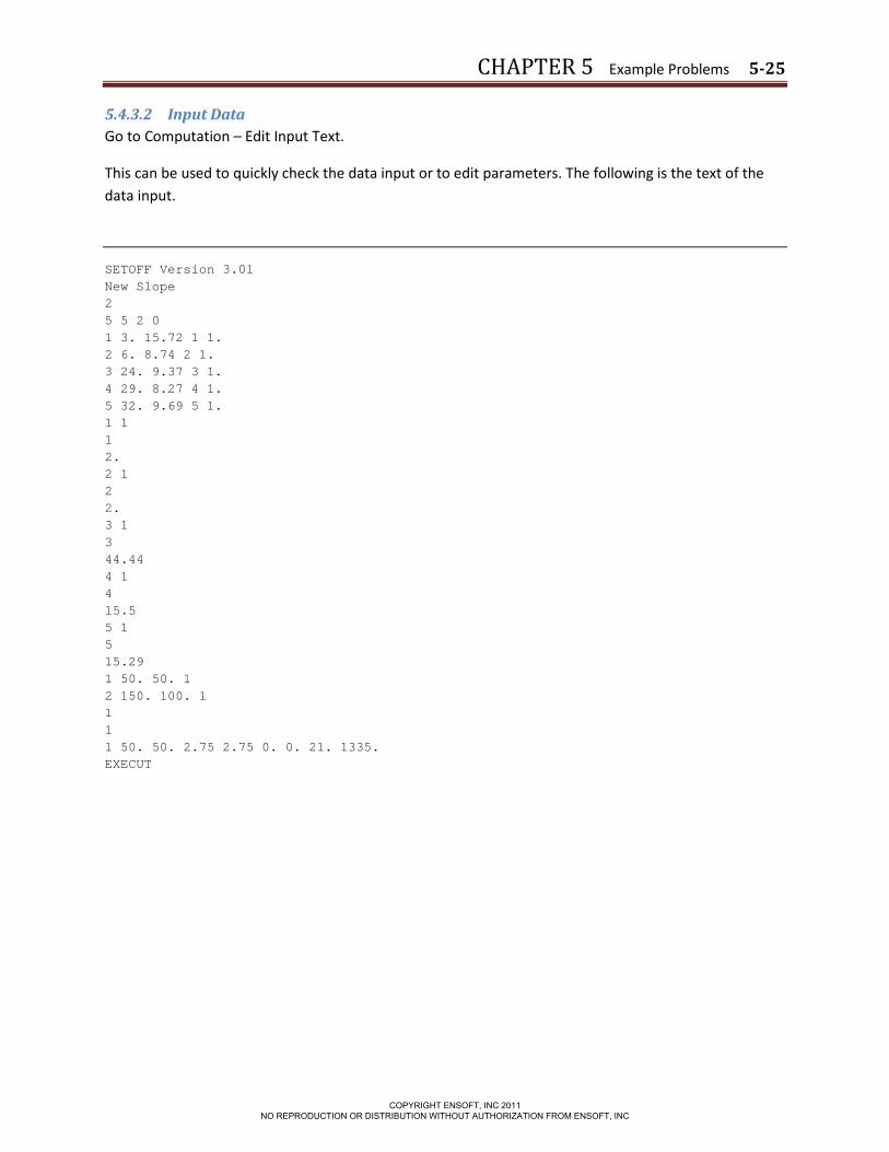
CHAPTER 5 Example Problems 5-25
5.4.3.2 Input Data Go to Computation – Edit Input Text.
This can be used to quickly check the data input or to edit parameters. The following is the text of the data input.
SETOFF Version 3.01 New Slope 2 5 5 2 0 1 3. 15.72 1 1. 2 6. 8.74 2 1. 3 24. 9.37 3 1. 4 29. 8.27 4 1. 5 32. 9.69 5 1. 1 1 1 2. 2 1 2 2. 3 1 3 44.44 4 1 4 15.5 5 1 5 15.29 1 50. 50. 1 2 150. 100. 1 1 1 1 50. 50. 2.75 2.75 0. 0. 21. 1335. EXECUT
COPYRIGHT ENSOFT, INC 2011 NO REPRODUCTION OR DISTRIBUTION WITHOUT AUTHORIZATION FROM ENSOFT, INC

CHAPTER 5 Example Problems 5-26
5.4.3.3 Output Results Go to Computation – View Output Text.
This is used to view the results of the analysis. The following is the text of the output results.
****************************************** * * * FOUNDATION SETTLEMENT ANALYSIS * * * ****************************************** SETOFF Version 3.01 New Slope TABLE 1 - PROBLEM CONTROL PARAMETERS COMPUTATION UNITS = 2 1 = U.S. GRAVITATIONAL SYSTEM 2 = S.I. ABSOLUTE SYSTEM NUMBER OF SOIL LAYERS = 5 NUMBER OF SOIL COMPRESSIBILITIES = 5 NUMBER OF SETTLEMENT POINTS = 2 NUMBER OF LOADED AREAS = 0 TABLE 2 - SOIL AND LAYER INFORMATION SOIL DEPTH TO LAYER LAYER MASS SOIL OVERBURDEN INIT VERTICAL SUBLAYER CENTER THICKNESS THICK. DENSITY COMP PRESSURE STRAIN (F0) NO. M M FACTOR KG/M**3 NO. KPA % 1 0.25 0.50 1.00 1603.00 1 3.930 0.000 2 0.75 0.50 1.00 1603.00 1 11.790 0.000 3 1.25 0.50 1.00 1603.00 1 19.650 0.000 4 1.75 0.50 1.00 1603.00 1 27.510 0.000 5 2.25 0.50 1.00 1603.00 1 35.370 0.000 6 2.75 0.50 1.00 1603.00 1 43.230 0.000 7 3.25 0.50 1.00 891.24 2 49.345 0.000 8 3.75 0.50 1.00 891.24 2 53.715 0.000 9 4.25 0.50 1.00 891.24 2 58.085 0.000 10 4.75 0.50 1.00 891.24 2 62.455 0.000 11 5.25 0.50 1.00 891.24 2 66.825 0.000 12 5.75 0.50 1.00 891.24 2 71.195 0.000 13 6.25 0.50 1.00 955.48 3 75.723 0.000 14 6.75 0.50 1.00 955.48 3 80.408 0.000 15 7.25 0.50 1.00 955.48 3 85.093 0.000 16 7.75 0.50 1.00 955.48 3 89.778 0.000 17 8.25 0.50 1.00 955.48 3 94.463 0.000
COPYRIGHT ENSOFT, INC 2011 NO REPRODUCTION OR DISTRIBUTION WITHOUT AUTHORIZATION FROM ENSOFT, INC

CHAPTER 5 Example Problems 5-27
18 8.75 0.50 1.00 955.48 3 99.148 0.000 19 9.25 0.50 1.00 955.48 3 103.833 0.000 20 9.75 0.50 1.00 955.48 3 108.518 0.000 21 10.25 0.50 1.00 955.48 3 113.203 0.000 22 10.75 0.50 1.00 955.48 3 117.888 0.000 23 11.25 0.50 1.00 955.48 3 122.573 0.000 24 11.75 0.50 1.00 955.48 3 127.258 0.000 25 12.25 0.50 1.00 955.48 3 131.943 0.000 26 12.75 0.50 1.00 955.48 3 136.628 0.000 27 13.25 0.50 1.00 955.48 3 141.313 0.000 28 13.75 0.50 1.00 955.48 3 145.998 0.000 29 14.25 0.50 1.00 955.48 3 150.683 0.000 30 14.75 0.50 1.00 955.48 3 155.368 0.000 31 15.25 0.50 1.00 955.48 3 160.053 0.000 32 15.75 0.50 1.00 955.48 3 164.738 0.000 33 16.25 0.50 1.00 955.48 3 169.423 0.000 34 16.75 0.50 1.00 955.48 3 174.108 0.000 35 17.25 0.50 1.00 955.48 3 178.793 0.000 36 17.75 0.50 1.00 955.48 3 183.478 0.000 37 18.25 0.50 1.00 955.48 3 188.163 0.000 38 18.75 0.50 1.00 955.48 3 192.848 0.000 39 19.25 0.50 1.00 955.48 3 197.533 0.000 40 19.75 0.50 1.00 955.48 3 202.218 0.000 41 20.25 0.50 1.00 955.48 3 206.903 0.000 42 20.75 0.50 1.00 955.48 3 211.588 0.000 43 21.25 0.50 1.00 955.48 3 216.273 0.000 44 21.75 0.50 1.00 955.48 3 220.958 0.000 45 22.25 0.50 1.00 955.48 3 225.643 0.000 46 22.75 0.50 1.00 955.48 3 230.328 0.000 47 23.25 0.50 1.00 955.48 3 235.013 0.000 48 23.75 0.50 1.00 955.48 3 239.698 0.000 49 24.25 0.50 1.00 843.31 4 244.108 0.000 50 24.75 0.50 1.00 843.31 4 248.243 0.000 51 25.25 0.50 1.00 843.31 4 252.378 0.000 52 25.75 0.50 1.00 843.31 4 256.513 0.000 53 26.25 0.50 1.00 843.31 4 260.648 0.000 54 26.75 0.50 1.00 843.31 4 264.783 0.000 55 27.25 0.50 1.00 843.31 4 268.918 0.000 56 27.75 0.50 1.00 843.31 4 273.053 0.000 57 28.25 0.50 1.00 843.31 4 277.189 0.000 58 28.75 0.50 1.00 843.31 4 281.324 0.000 59 29.25 0.50 1.00 988.11 5 285.814 0.000 60 29.75 0.50 1.00 988.11 5 290.659 0.000 61 30.25 0.50 1.00 988.11 5 295.504 0.000 62 30.75 0.50 1.00 988.11 5 300.349 0.000 63 31.25 0.50 1.00 988.11 5 305.194 0.000 64 31.75 0.50 1.00 988.11 5 310.039 0.000
COPYRIGHT ENSOFT, INC 2011 NO REPRODUCTION OR DISTRIBUTION WITHOUT AUTHORIZATION FROM ENSOFT, INC

CHAPTER 5 Example Problems 5-28
****************************************** * * * FOUNDATION SETTLEMENT ANALYSIS * * * ****************************************** SETOFF Version 3.01 New Slope TABLE 3 - SOIL COMPRESSIBILITY SOURCE AND DATA SOIL COMPRESSIBILITY NO. 1 1 THE SLOPE OF THE F(%)-LOG P CURVE IS 2.000 SOIL COMPRESSIBILITY NO. 2 2 THE SLOPE OF THE F(%)-LOG P CURVE IS 2.000 SOIL COMPRESSIBILITY NO. 3 3 THE SLOPE OF THE F(%)-LOG P CURVE IS 44.440 SOIL COMPRESSIBILITY NO. 4 4 THE SLOPE OF THE F(%)-LOG P CURVE IS 15.500 SOIL COMPRESSIBILITY NO. 5 5 THE SLOPE OF THE F(%)-LOG P CURVE IS 15.290
COPYRIGHT ENSOFT, INC 2011 NO REPRODUCTION OR DISTRIBUTION WITHOUT AUTHORIZATION FROM ENSOFT, INC

CHAPTER 5 Example Problems 5-29
****************************************** * * * FOUNDATION SETTLEMENT ANALYSIS * * * ****************************************** SETOFF Version 3.01 New Slope TABLE 4 - SETTLEMENT POINT DATA POINT POINT COORDINATES LAYER NO, X Y NO.* M M 1 50.00 50.00 1 2 150.00 100.00 1 * NUMBER OF SOIL LAYER AT WHICH SETTLEMENT COMPUTATION BEGINS 1 3 0 1
COPYRIGHT ENSOFT, INC 2011 NO REPRODUCTION OR DISTRIBUTION WITHOUT AUTHORIZATION FROM ENSOFT, INC

CHAPTER 5 Example Problems 5-30
1 ****************************************** * * * FOUNDATION SETTLEMENT ANALYSIS * * * ****************************************** SETOFF Version 3.01 New Slope TABLE 6 = AVERAGE STRESS INCREASE SETTLEMENT POINT NO. 1 2 DEPTH, M STRESS, KPA 0.25 21.064 0.000 0.75 109.537 0.000 1.25 83.765 0.000 1.75 66.127 0.000 2.25 53.525 0.000 2.75 44.215 0.000 3.25 37.137 0.000 3.75 31.633 0.000 4.25 27.270 0.000 4.75 23.750 0.000 5.25 20.873 0.000 5.75 18.492 0.000 6.25 16.487 0.000 6.75 14.798 0.000 7.25 13.346 0.000 7.75 12.113 0.000 8.25 11.034 0.000 8.75 10.097 0.000
COPYRIGHT ENSOFT, INC 2011 NO REPRODUCTION OR DISTRIBUTION WITHOUT AUTHORIZATION FROM ENSOFT, INC

CHAPTER 5 Example Problems 5-31
1 ****************************************** * * * FOUNDATION SETTLEMENT ANALYSIS * * * ****************************************** SETOFF Version 3.01 New Slope TABLE 6 = AVERAGE STRESS INCREASE (CONT) SETTLEMENT POINT NO. 1 2 DEPTH, M STRESS, KPA 9.25 9.269 0.000 9.75 8.537 0.000 10.25 7.894 0.000 10.75 7.318 0.000 11.25 6.808 0.000 11.75 6.343 0.000 12.25 5.927 0.000 12.75 5.554 0.000 13.25 5.209 0.000 13.75 4.899 0.000 14.25 4.619 0.000 14.75 4.354 0.000 15.25 4.114 0.000 15.75 3.898 0.000 16.25 3.696 0.000 16.75 3.500 0.000 17.25 3.326 0.000 17.75 3.166 0.000
COPYRIGHT ENSOFT, INC 2011 NO REPRODUCTION OR DISTRIBUTION WITHOUT AUTHORIZATION FROM ENSOFT, INC

CHAPTER 5 Example Problems 5-32
1 ****************************************** * * * FOUNDATION SETTLEMENT ANALYSIS * * * ****************************************** SETOFF Version 3.01 New Slope TABLE 6 = AVERAGE STRESS INCREASE (CONT) SETTLEMENT POINT NO. 1 2 DEPTH, M STRESS, KPA 18.25 3.019 0.000 18.75 2.884 0.000 19.25 2.750 0.000 19.75 2.630 0.000 20.25 2.521 0.000 20.75 2.414 0.000 21.25 2.312 0.000 21.75 2.218 0.000 22.25 2.125 0.000 22.75 2.043 0.000 23.25 1.965 0.000 23.75 1.896 0.000 24.25 1.827 0.000 24.75 1.760 0.000 25.25 1.695 0.000 25.75 1.640 0.000 26.25 1.575 0.000 26.75 1.522 0.000
COPYRIGHT ENSOFT, INC 2011 NO REPRODUCTION OR DISTRIBUTION WITHOUT AUTHORIZATION FROM ENSOFT, INC

CHAPTER 5 Example Problems 5-33
1 ****************************************** * * * FOUNDATION SETTLEMENT ANALYSIS * * * ****************************************** SETOFF Version 3.01 New Slope TABLE 6 = AVERAGE STRESS INCREASE (CONT) SETTLEMENT POINT NO. 1 2 DEPTH, M STRESS, KPA 27.25 1.480 0.000 27.75 1.428 0.000 28.25 1.386 0.000 28.75 1.337 0.000 29.25 1.297 0.000 29.75 1.257 0.000 30.25 1.217 0.000 30.75 1.186 0.000 31.25 1.148 0.000 31.75 1.119 0.000
COPYRIGHT ENSOFT, INC 2011 NO REPRODUCTION OR DISTRIBUTION WITHOUT AUTHORIZATION FROM ENSOFT, INC

CHAPTER 5 Example Problems 5-34
****************************************** * * * FOUNDATION SETTLEMENT ANALYSIS * * * ****************************************** SETOFF Version 3.01 New Slope TABLE 7 - COMPUTED SETTLEMENT IN MILLIMETRES SETTLEMENT POINT NO. 1 2 DEPTH, M 0.250 8.034 0.000 0.750 10.124 0.000 1.250 7.212 0.000 1.750 5.320 0.000 2.250 4.002 0.000 2.750 3.059 0.000 3.250 2.437 0.000 3.750 2.011 0.000 4.250 1.672 0.000 4.750 1.400 0.000 5.250 1.180 0.000 5.750 1.003 0.000 6.250 19.010 0.000 6.750 16.302 0.000 7.250 14.059 0.000 7.750 12.213 0.000 8.250 10.661 0.000 8.750 9.359 0.000
COPYRIGHT ENSOFT, INC 2011 NO REPRODUCTION OR DISTRIBUTION WITHOUT AUTHORIZATION FROM ENSOFT, INC

CHAPTER 5 Example Problems 5-35
****************************************** * * * FOUNDATION SETTLEMENT ANALYSIS * * * ****************************************** SETOFF Version 3.01 New Slope TABLE 7 - COMPUTED SETTLEMENT IN MILLIMETRES(CONT) SETTLEMENT POINT NO. 1 2 DEPTH, M 9.250 8.252 0.000 9.750 7.308 0.000 10.250 6.505 0.000 10.750 5.812 0.000 11.250 5.217 0.000 11.750 4.694 0.000 12.250 4.241 0.000 12.750 3.845 0.000 13.250 3.493 0.000 13.750 3.185 0.000 14.250 2.914 0.000 14.750 2.667 0.000 15.250 2.449 0.000 15.750 2.257 0.000 16.250 2.082 0.000 16.750 1.921 0.000 17.250 1.779 0.000 17.750 1.651 0.000
COPYRIGHT ENSOFT, INC 2011 NO REPRODUCTION OR DISTRIBUTION WITHOUT AUTHORIZATION FROM ENSOFT, INC

CHAPTER 5 Example Problems 5-36
****************************************** * * * FOUNDATION SETTLEMENT ANALYSIS * * * ****************************************** SETOFF Version 3.01 New Slope TABLE 7 - COMPUTED SETTLEMENT IN MILLIMETRES(CONT) SETTLEMENT POINT NO. 1 2 DEPTH, M 18.250 1.536 0.000 18.750 1.432 0.000 19.250 1.334 0.000 19.750 1.247 0.000 20.250 1.169 0.000 20.750 1.095 0.000 21.250 1.026 0.000 21.750 0.964 0.000 22.250 0.904 0.000 22.750 0.852 0.000 23.250 0.803 0.000 23.750 0.760 0.000 24.250 0.251 0.000 24.750 0.238 0.000 25.250 0.225 0.000 25.750 0.214 0.000 26.250 0.203 0.000 26.750 0.193 0.000
COPYRIGHT ENSOFT, INC 2011 NO REPRODUCTION OR DISTRIBUTION WITHOUT AUTHORIZATION FROM ENSOFT, INC

CHAPTER 5 Example Problems 5-37
****************************************** * * * FOUNDATION SETTLEMENT ANALYSIS * * * ****************************************** SETOFF Version 3.01 New Slope TABLE 7 - COMPUTED SETTLEMENT IN MILLIMETRES(CONT) SETTLEMENT POINT NO. 1 2 DEPTH, M 27.250 0.185 0.000 27.750 0.176 0.000 28.250 0.168 0.000 28.750 0.160 0.000 29.250 0.150 0.000 29.750 0.143 0.000 30.250 0.136 0.000 30.750 0.131 0.000 31.250 0.125 0.000 31.750 0.120 0.000 TOTAL(mm) 215.270 0.000
COPYRIGHT ENSOFT, INC 2011 NO REPRODUCTION OR DISTRIBUTION WITHOUT AUTHORIZATION FROM ENSOFT, INC