Copyright 2002, Society of Petroleum Engineers Inc. This paper was prepared for presentation at the 2002 SPE Electrical Submersible Pump Workshop held in Houston, Texas, May1 – May 3 2002. This paper was selected for presentation by an SPE Program Committee following review of information contained in an abstract submitted by the author(s). Contents of the paper, as presented, have not been reviewed by the Society of Petroleum Engineers and are subject to correction by the author(s). The material, as presented, does not necessarily reflect any position of the Society of Petroleum Engineers, its officers, or members. Papers presented at SPE meetings are subject to publication review by Editorial Committees of the Society of Petroleum Engineers. Electronic reproduction, distribution, or storage of any part of this paper for commercial purposes without the written consent of the Society of Petroleum Engineers is prohibited. Permission to reproduce in print is restricted to an abstract of not more than 300 words; illustrations may not be copied. The abstract must contain conspicuous acknowledgment of where and by whom the paper was presented. Write Librarian, SPE, P.O. Box 833836, Richardson, TX 75083-3836, U.S.A., fax 01-972-952-9435.

Abstract Electrical submersible pumps (ESP’s) are very successful

in pumping low viscosity fluids. For certain applications, production conditions may result in a gas-liquid flow inside the pump. This may be due to different reservoir and fluid properties as compared to design conditions or changes in the operational parameters of the system. The two-phase flow behavior of centrifugal impellers and diffusers is significantly different from the single-phase behavior. Knowledge of the two-phase flow behavior of ESP stages is then of paramount importance for the design, optimization and troubleshooting of this artificial lift method for those conditions.

It is well known that predicting the two-phase behavior of a centrifugal pump is a very complex task dependent on several variables such as the amount of gas, intake pressure and pump geometry. Modeling multiphase flow inside turbo machines is still an open problem with several unresolved issues related to numerical algorithms, closer and constitutive equations for interfacial transfer terms and turbulence behavior of multiphase flow in non-circular curved rotating channels.

Due to those complex difficulties currently no single model or general correlation is available to predict performance of pumps under multi-phase conditions. The homogeneous model currently used in the industry assumes that the two-phase flow performance of the stage is obtained by correcting the single-phase performance to account for the mixture density and total mixture volumetric flow rate. The predictions based on this simple approach are of limited

validity and applicable only for low intake gas void fractions. Extension of this model to higher gas void fractions may result in erroneous predictions. Moreover, this approach does not predict surging and gas locking conditions which are important two-phase flow phenomena that affects the pump performance.

Several investigators have addressed those problems experimentally seeking correlations to predict those phenomena. The correlations developed are based on an average performance of a certain specific pump with a fixed number of stages. As a consequence those correlations are not only limited to the specific impeller and stage design tested but are also influenced by the number of stages used.

As the two-phase flow mixture flows across stages in a multi-stage pump, pressure, temperature and gas liquid equilibrium changes. Progressively towards the final stages, the conditions will be considerably different from the conditions prevailing at the initial stages.

To understand this stage wise behavior, The University of Tulsa Artificial Lift Projects � TUALP is currently pursuing a research line both on the experimental and theoretical aspects of the problem. A new state of the art experimental setup was built in order to investigate the real multiphase performance of a commercial 22 stages mixed design pump.

This paper presents the experimental results of tests conducted at TUALP on a 22-stage pump at 100-psia intake pressure. A complete map of the two-phase flow behavior on stage wise basis including the head degradation, surging and gas locking is presented. The averaged efficiency of the pump under multiphase flow conditions has been mapped for that intake pressure. This paper also presents a comprehensive literature review of previous research on this topic.

Introduction

Centrifugal pumps are dynamic single or multistage devices that use kinetic energy to increase liquid pressure. Current impellers and diffuser designs are very successful in handling low viscous, single-phase incompressible fluids, but

SPE

Two-Phase Flow Performance of Electrical Submersible Pump Stages - Experimental Investigation and Literature Review of Predictive Methods Rui Pessoa, SPE, PDVSA-Intevep, Raghavan Beltur and Mauricio Prado, SPE, The University of Tulsa

2 RUI PESSOA, RAGHAVAN BELTUR AND MAURICIO PRADO SPE

are severely impacted by free gas, highly compressible or viscous fluids.

Each type of pump has a specific single-phase performance curve, which indicates the relationship between the head developed by the pump and the flow rate through the pump for a certain rotational speed. Traditionally this curve is experimentally determined using water as the working fluid. The head performance curves are valid then for any other low viscosity single-phase liquid independent of its density. Other curves such as the brake horsepower and efficiency are usually also presented on the same chart. In the case of multi-stage pumps handling incompressible fluids, the performance is presented on average per stage. An example of these performance curves is shown in Fig. 1. Two vertical lines define the lower and upper limits where it is recommended to operate the equipment. The point of maximum efficiency within the operating range is called the best efficiency point, usually abbreviated as BEP.

The sizing of a multi-stage ESP has shown good agreement for low viscosity oil wells with no free gas or very low volumetric free gas fractions (< 2%) at pump intake conditions based on the water performance curves supplied by the manufacturer.

While handling higher contents of free gas the centrifugal pump suffers head degradation and the manufacturer single-phase water performance curves cannot be used. Additionally, to performance degradation while handling free gas, submersible pumps also require prediction of surging and gas lock conditions. Surging is a phenomenon related to instability of the pump performance and has been observed in the lower flow rate region of the pump. Surging is a cyclic fluctuation of the system�s pressure and is associated with a positive slope of the head vs flow rate performance curve. It is also known in literature as heading. The term instability is also used in the technical literature in reference to this phenomenon. Studies from nuclear industry, states that surging appears as a discontinuity in the head performance and such discontinuity is a consequence of a continuous change in flow pattern from dispersed bubble or turbulent churned flow to stratified or plug flow of gas. This abrupt fluctuation in performance is observed for flow rates smaller than best efficiency point and changes with the amount of gas at the intake. The pressure fluctuation during surging with respect to time is shown in Fig. 2. Some authors refer it to reverse flow as during surging even the intake pressure begins to fluctuate. In the field surging can be observed as a wide band in power consumption chart as the motor load varies continuously.

The next deteriorating stage after surging is gas lock. This is the condition where a pump stops delivering head. Gas lock is related to the maximum free gas volume and liquid flow rate that a pump can handle under certain conditions where it suffers a sharp decrease on the head performance and stops generating head. Before the gas locking occurs there is one more phenomenon called gas blocking, during which gas

accumulates at the center of the impeller reducing the effective suction flow area for liquid, resulting in reduction of head performance. As the gas percentage increases more and more eye area of impeller is occupied by gas resulting in reduction of head performance of pump leading to gas locking. Once the pump gets locked, it could be brought to normal operating condition by either increasing intake pressure or by stopping the pump so that gas is pushed out of suction by liquid.

A comparison between the experimentally determined head performance for the pump used in this study and the predicted performance using the homogeneous model based is shown in Fig. 3. We can see that actual two-phase flow performance is considerably different from the single-phase and from the homogenous model prediction. In order to correctly design, analyze and troubleshoot ESP applications in gassy environments the performance of ESP under multiphase conditions must be known. In order to achieve this objective extensive theoretical and experimental research must be conducted to better understand this complex phenomenon.

The rest of this paper is organized in the flowing sections:

Basic Concepts. Presents the definition of single and two-phase head, pressure based on insitu and surface conditions. Also clarifies the terminology defined by different researches.

Homogeneous model. Presents in detail the homogeneous model procedure for predicting two-phase flow performance of ESP.

Literature Review. Presents a review of previous works related to multiphase performance of ESPs. In this paper a review of the experimental works of Dunbar (1989), Lea & Bearden (1982), Turpin (1986), Cirilo (1998) and Romero (1999) are presented.

Experimental Work. This section presents detail of the experimental work conducted in this research covering the experimental facilities, customization of the pump, experimental procedure and experiment matrix as well as the results.

Conclusion and Recommendations. Those two sections present a summary of the paper with its main important conclusions and lay out the necessary steps for further improvement of the experimental program.

Basic Concepts The Bernoulli�s equation states that for the fluid flowing through the frictionless pipe the fluid energy E , at any point in pipe remains constant and with the mass m and gravity acceleration g , equation can be expressed as:

constantVmPmgmgZ =++2

2

γ (1)

In Eq. 1, the first term is known as potential energy of the fluid and the third term is known as kinetic energy of the fluid.

SPE Two-Phase Flow Performance of Electrical Submersible Pump Stages - Experimental Investigation and Literature Review of Predictive Methods 3

It is the second term, pressure energy that is important to explain and evaluate the frictionless performance of centrifugal pumps.

The ideal performance of the centrifugal pumps considering no pre-rotation of fluids entering the impeller and no frictional losses along the impeller and diffuser channel is given by:

)tan(1

222

idc

llidlstage h

qrPβπ

ωρωρ −=∆ (2)

where stageP∆ is the average pressure increment per stage of

the pump, lρ is the liquid density, ω is the angular velocity

or rotational speed of impeller, lq is the liquid flow rate, idβ

is the angle at the discharge of impeller or discharge angle,

ch is the height of channel and idr is the impeller discharge radius.

It is evident from the Eq. 2 that the pressure increment developed is only function of the liquid density and flow rate. The other parameters are geometric and remain constant for a particular pump rotating at a given speed.

},{ llstagestage qPP ρ∆=∆ (3)

The ideal liquid head performance stageH of a centrifugal

pump is given as the ratio of pressure increment P∆ to the product of liquid density lρ and gravity acceleration g .

gPH

lstage ρ

∆= (4)

Re-writing Eq. 2 to calculate the pressure head stageH developed by one stage, we obtain:

)tan(1

2

22

idcl

idstage gh

qgrH

βπωω

−= (5)

From Eq. 5 we see that the ideal head becomes independent of fluid density and is function only of liquid flow rate.

}{ lstagestage qHH = (6)

For a fixed fluid flow rate, the pressure increment is only function of fluid density as shown in Eq. 3. In other words, pressure increment developed by the pump varies with fluid density but the head developed remains constant for a given flow rate. This concept of constant head is illustrated in Fig. 4.

Pressure performance for other low viscosity liquids is calculated by:

SGgqHqP wlstagellstage ρρ }{},{ =∆ , (7)

where wρ is the water density and SG is the fluid specific gravity.

Since head, stageH , developed for incompressible fluids is a

function only of liquid flow rate lq , Eq. 6 can be used for any single-phase incompressible, low viscosity fluid. For multi-stage pumps the pump head can be obtained by multiplying stage head by the number of stages, n .

}{}{ lstagelpump qHnqH = (8)

in a similar way the pump pressure increment is:

SGgqHnqP wlstagellpump ρρ }{},{ =∆ (9)

When pumping slightly compressible fluids with small number of stages, Eqs. 8 and 9 can be used to calculate head and pressure increments. This can be used as a good approximation since pressure raise across each stage is generally small and compressibility effects can be neglected inside the stage or across the pump.

For a pump with a larger number of stages, continuous increase in pressure will change the liquid flow rates and densities across the pump. Each stage still can be modeled using Eq. 6, since the pressure increment across each stage is small. On the other hand, as the intake conditions vary stage by stage, Eqs. 8 and 9 cannot be used to calculate overall pump performance.

Due to compressibility effects, the density lρ and flow

rate lq changes across each stage. The stage head must then take into account the actual insitu flow rate and can be expressed also as a function of the standard conditions flow rate sc

lq and the in situ pressure P:

},{ Pqqq sclll = (10)

},{}{ PqHqH sclstagelstage = (11)

The overall head developed by a pump with n stages can be obtained as summation of performance of each individual stage and is given by:

∑∑ ==n

sclstage

n

lstagelpump PqHqHqH11

},{}{}{ (12)

And similarly the total pressure developed by pump can be expressed as:

}{},{},{1

PgPqHqPn

sclstagelpump ρρ ∑=∆ (13)

Now we can draw attention to the problem of ESP performance when handling two-phase flow. The two-phase flow performance of ESP is considerably different than the single-phase performance. Not only the gas phase is a very

4 RUI PESSOA, RAGHAVAN BELTUR AND MAURICIO PRADO SPE

compressible phase, but also the mixture compressibility will be function of the actual slippage conditions and flow pattern inside the ESP impeller and diffuser channels. As a consequence we anticipate the multiphase performance of ESP to be function not only of the gas and liquid flow rates but also of all variables known to influence the flow field of multiphase mixtures, such as fluid densities, viscosity, interfacial tension, bubble or droplet size flow pattern, interfacial area concentration, turbulence density, etc�.

While designing or selecting a pump with large number of stages, the effect of pressure on density over each stage needs to be considered. The total pressure increment for a pump with n number of stages is expressed as summation of each stage pressure increment:

},,{1

iscg

scl

tpstage

ntppump PqqPP ∆=∆ ∑ (14)

And in terms of stage head and mixture density the total pressure developed by a pump can be expressed as:

gPqqHPn

slipnomi

scg

scl

tpstage

tppump ∑=∆

1

},,{ ρ (15)

The no slip mixture density is chosen for convenience and is a function of flow rates and intake pressure.

},,{ iscg

scl

slipnom

slipnom Pqqρρ = (16)

The mixture density in terms of gas void fraction can also be expressed as:

gglgslipno

m ρλρλρ +−= )1( (17)

where the no slip gas void fraction, which varies between 0 and 1, is given as:

lg

gg qq

q+

=λ (18)

Many authors have reported their work on free gas liquid ratio, FGLR, which is defined as the ratio of free gas flow rate to the liquid flow rate. Its value varies between 0 and infinity.

l

g

qq

FGLR = (19)

The no slip gas void fraction gλ can be related to the free gas liquid ratio by;

1+=

FGLRFGLR

gλ (20)

and in turn FGLR can be expressed as:

g

gFGLRλ

λ−

=1

(21)

The condition will be more complex in field application as gas is miscible in oil and the process of transient gas solubility inside the pump is not well understood yet.

As a conclusion, predicting the performance of ESP�s under two-phase conditions is a complex and challenging problem. It requires accurate data and good understanding of physical and chemical properties of the mixture in use.

Homogeneous Model The traditional method for predicting the two-phase

performance of ESP pump is based on the homogeneous model. In this model the two-phase mixture is assumed to behave as a homogeneous fluid. The total mixture flow rate is then the sum of the liquid flow rate and gas flow rate. The mixture flow rate mq is expressed as:

glm qqq += (22)

Considering these assumptions, the two-phase stage head developed can be expressed as head of single-phase at total mixture flow rate:

mqspstage

tpstage HH @= (23)

Similarly the two-phase stage pressure increment can be written as:

slipnom

qspstage

tpstage gHP m ρ@=∆ (24)

As per the homogeneous model, two-phase stage head is equal to single�phase head at total mixture flow rate. The two-phase stage head can be expressed as function of liquid flow rate and gas void fraction gλ .

mqspstagegl

tpstage

tpstage HqHH @},{ == λ (25)

The mixture flow rate can be expressed in terms of gas void fraction gλ as:

mg

llg q

qqq =

−=+

λ1 (26)

Now the two-phase stage head increment can be written as:

mqspstagegl

tpstage HqH @},{ =λ (27)

The two-phase head prediction based on single-phase head provided by manufacturer using Eq. 27 is demonstrated in Fig. 5. The Fig. 6 shows an example of the two-phase head based on single-phase head for different gas void fractions for a specific pump.

As said before, the stage head is related to a certain reference density; in this case it is the no slip mixture density. The stage pressure increment is obtained as:

SPE Two-Phase Flow Performance of Electrical Submersible Pump Stages - Experimental Investigation and Literature Review of Predictive Methods 5

slipnom

tpstage

tpstage gHP ρ=∆ (28)

It is useful to compare the stage head with the manufacturer single-phase water head based on the same density reference. If we use the water density as a reference for the stage two-phase flow head we obtain:

wtpwater

tpstage gHP ρ=∆ (29)

where tpwaterH is the two-phase head based on the water density.

The relationship between the two definitions of stage two-phase flow head becomes:

wtpwater

slipnom

tpstage HH ρρ = (30)

The above equation can be expressed also as:

mqspstage

w

slipnomtp

water HH @

=

ρρ (31)

Re-writing the equation we have two-phase water head as:

mqspstage

w

ggg

tpwater HH @)1(

+−=

ρρλ

λ (32)

The two-phase water head prediction based on single-phase head provided by manufacturer using Eq. 31 is demonstrated in Fig. 7. The Fig. 8 shows an example of the two-phase head based on single-phase head for different gas void fractions for a specific pump.

It appears from Fig. 8 that there is some head degradation using this method. In reality what Fig. 8 is showing is degradation in pressure due to the reduction in mixture density, which was expected, but remember that in the homogeneous model no degradation is accounted in the head performance as indicated by Eq. 27.

The head prediction based on homogeneous model provides a good approximation when the mixture is homogeneous inside the pump. Homogeneous flow can occur only at low gas void fractions. The effect of two-phase flow results in some head degradation and other complex two-phase flow phenomena at higher void fractions.

The comparison of two-phase experimental results with the homogeneous method head performance is shown in Fig. 3. This figure shows the considerable head degradation that exists for higher gas void fractions not captured by the homogeneous model and the difference between the experimental and predicted surging points. Literature Review

Dunbar (1989) presented a paper, focusing on the operational conditions of GLR and pump intake pressures where the homogeneous model could successfully be applied to design ESP�s.

Dunbar constructed a reference curve called �Dunbar Curve� shown in Fig. 9. This shows plot a for the minimum intake pressure that should be attained for a given gas liquid ratio, to apply homogeneous model or to account for no head degradation. The term �without correcting the pump performance� mentioned in Dunbar�s paper should not be confused with single-phase liquid performance of the pump. This term refers to the two-phase head prediction based on the homogeneous model presented.

The region above the Dunbar curve in Fig. 9, referred as �OK for Pumping� by the author is the region where the homogeneous model can be applied. Here in this region the minimum intake pressure condition for a specific vapor liquid ratio (V/L) is satisfied. The region below the Dunbar curve referred as �not OK for pumping� by the author is the region where the homogeneous model cannot be applied to predict pump performance. For the operating conditions below Dunbar curve head degradation should be accounted. To account for head degradation Dunbar defines two auxiliary factors ALIM and BLIM. ALIM is the value of vapor liquid ratio on the Dunbar curve for the operating intake pressure where no head degradation is expected. BLIM is the value of maximum vapor liquid ratio for the operating intake pressure where the pump generates no head. This point can also be referred to as gas locking. Unfortunately the author does not provide any correlation or criteria to determine the value of BLIM and advises to rely on the experimental data or experience. The head degradation below the Dunbar curve is given as a linear function from ALIM to BLIM. Just for didactic purpose an imaginary curve is shown in Fig. 9 to represent the zero performance or BLIM curve. (This imaginary curve is not part of the original plot).

The best curve fit equation for Dunbar curve or ALIM obtained in this work is given by:

( ) 724.1/1min 935 FGLRPi = (33)

where miniP is the minimum intake pressure that should be

attained for a given FGLR to apply the homogeneous model.

The graph in Fig. 9 presents the Dunbar curve superimposed with value of V/L ratio that might exists at the pump intake for certain application. The 10% GIP curve is shown with 90% efficiency of gas separation. The GIP or Gas Ingestion Percentage curves shown in Fig. 9 is calculated based on PVT data with an oil of 21 °API, gas specific gravity of 0.7, bottom hole temperature of 200 °F, GOR of 350 scf/stb and water cut of 50%. For the data plotted the bubble point pressure is 2600 psi. The GIP curves can be obtained for other fluids and separator efficiency.

The homogeneous model can be applied for the operating conditions in the shaded region above the Dunbar curve. Here in this region no head degradation is expected. For the operating condition below the Dunbar curve head degradation should be accounted as explained earlier. Below the BLIM no head is generated and requires a suitable gas separator to

6 RUI PESSOA, RAGHAVAN BELTUR AND MAURICIO PRADO SPE

modify the intake condition so that operating condition falls at least above the BLIM curve. Using a gas separator for operating conditions above Dunbar curve will help in increasing mixture density and in turn the pump will generate higher-pressure increment. Effect of separators on performance of ESP depends upon where the operating conditions fall into after gas separation. In the region between ALIM and BLIM, the effect of gas separators will reduce the head degradation.

As a practice Dunbar factor curve should not be considered as a precise curve but merely a trend curve to be used as a guide, as pointed by the author.

An important contribution of Dunbar approach is the general criteria for application of homogeneous model for head prediction in two-phase flow. But the validity of this approach for different types of pump must be investigated. More over no criteria or model is given to predict BLIM. Also, surging conditions were not considered.

Lea and Bearden (1982) conducted experiments on I-42B, C-72 radial flow type pumps and K-70 mixed flow type using air-water and diesel-CO2 as test fluids. Experiments were conducted to map the pump performance varying intake pressure and gas void fraction. The authors also compared the performance of axial flow type pumps with mixed flow type pumps.

Test results on I-42B radial pump with water-air, are shown in Fig. 10. The tests were conducted at only 25-psig intake pressure due equipment pressure rating restrictions. Results show the gradual decay of two-phase head performance with increase in gas void fraction. The head performance begins to departure severely from the water curve at 7% free gas fraction. Fluctuation of pressure increment was observed at 11% free gas void fraction.

The test results on I-42B radial pump with CO2 and Diesel are shown in Figs. 11, 12 and 13 based on mixture density at average pump pressure and temperature condition. It can be seen here that with the increase in intake pressure, the head performance improves and move towards the single-phase curve. Similar observation can also be made with the results of C-72 radial type pump shown in Fig. 14 and 15.

C-72 radial type and K-70 mixed flow type pump were selected to compare the results of different types of pumps, as the best efficiency point for both pumps is almost the same. Now comparing results shown in Fig. 16 and 17 of K-70 mixed type pump with the results of C-72 radial type pump shown in Fig. 14 and 15, it is clear that the average stage pressure increment is better with mixed flow type pump. With the mixed flow type pump, the stable operating range for liquid flow rate improves with the increase in intake pressure and also surging region moves towards smaller liquid flow rates. Similar trends were not observed with both models of radial type pumps.

At low gas fractions (10% at 50 and 100 psig intake pressure) the calculated head values are above the diesel base curve. This might be due to errors in calculation of mixture

density, as solubility of CO2 in diesel within short period of time due to turbulence inside the pump is not clearly understood. Though separate tests were conducted to study the solubility, the process was different, time consuming and over fixed gas liquid contact area.

This study provided the following conclusions:

For a constant gas fraction at pump intake, head degradation decreases as the intake pressure increases.

The flow conditions become unstable when the gas at the pump intake exceeds certain critical limits. For the air-water tests, the critical limit was approximately 10% gas by volume at 25-psig of intake pressure. For the Diesel-CO2 tests, the critical limit was found to be about 15% at 50 psig.

Pump performance also depends on the stage geometry and hydraulic design. The mixed flow impeller style pumps handle gaseous fluids better than the radial stage style pumps. Also, for similar intake pressures and gas fractions, pump operation was found to be more stable when operating to the right of the best efficiency point (BEP).

Turpin (1986) developed a correlation, which would predict the head capacity performance of the electrical submersible pump as a function of gas liquid ratio, suction pressure and liquid flow rate.

Experimental data used by Turpin to develop model were collected by Lea and Bearden (1982) presented in previous section. Turpin considers that the controlling factors for performance of pumps are the in-situ gas liquid ratio (FGLR) at the intake condition, the intake pressure and the liquid flow rate.

Turpin has obtained one correlation for both I-42B radial and K-70 mixed flow pump, which are of different geometric design and have different best efficiency points. The resulting correlation for I-42B and K-70 pumps is given as:

)/( lg qqasp

tp

eHH −= (34)

or

)(FGLRasp

tp

eHH −= (35)

where tpH is the two-phase head, spH is the single-phase liquid head at liquid flow rate lq , gq and lq are the in-situ volumetric flow rate of gas and liquid respectively, at the suction of the pump and iP is the absolute suction pressure at the intake.

The parameter a is given by:

il

g

i Pqq

Pa

4103464302 −

= (36)

SPE Two-Phase Flow Performance of Electrical Submersible Pump Stages - Experimental Investigation and Literature Review of Predictive Methods 7

A second correlation was developed to quantify the region of unacceptable pump performance. This was done by ploting the pump performance at various combinations of gas-liquid ratio and suction pressure. The quantity φ is given as;

=

i

lg

Pqq

3/

2000φ (37)

The plots in Fig. 18 and 19 for two-phase head prediction are based on the correlation developed for I-42B and K-70 pumps. It predicts and converges to maximum liquid flow rate contrary to maximum liquid flow rate decreases with increase in gas volume at intake. And also as the value of φ reduces the head prediction curve move towards and goes beyond the water curve which is not acceptable.

It is well doccumented that two-phase performance is always smaller than the single-phase performance. Referring back to Eq. 34, the two-phase head is predicted with the exponential term. To satisfy this condition the term )/( lg qqae− should be less than 1 and the exponential power term

)/( gl qqa− should be negative. Then with algebraic manipulation it can be shown that the correlation developed for radial pumps I-42B and C-72 is only valid for

17890.0 ≤< φ .

For C-72 mixed type pump similar correlations are given as:

])(0001.0

)(00275.0

)(0258.01[

3

2

)(2

Dl

Dl

Dlqqa

sp

tp

Qq

Qq

QqeHH

lg

−−

−+

−−= −

(38)

or it can be expressed as:

[ ]KeHH

lg qqasp

tp)(2−= (39)

where K is:

])(0001.0

)(00275.0

)(0258.01[

3

2

Dl

Dl

Dl

QqQq

QqK

−−

−+

−−= (40)

The relations for a2 and QD are given respectively by,

=

l

g

i qq

Pa 22

285340 (41)

and

φ3.333.98 −=DQ (42) The correlation for different values of φ and experimental

data for the C-72 mixed type of pump is shown in Fig. 20. As observed in earlier correlation for radial pumps the head prediction curve does not converge to maximum single-phase flow rate. As the value of φ increases the maximum liquid flow rate is reducing. While re-plotting correlations, shown in

Fig. 20 it was observed that the correlation does not reproduce the single-phase curve with φ zero.

For the values of φ smaller than 0.2545, the maximum liquid flow rate predicted is higher than the maximum single-phase liquid flow rate of 119.90 gpm and for the value of K>0.92 head prediction shows the weird behavior. Based on this K value, the minimum liquid flow rate to which correlation is valid can be expressed as:

φφ 3.3322.105min −== ll qq (43)

To conclude, the Turpin�s correlations for the radial type pump C-72 are valid only for values 12545.0 ≤< φ and for liquid flow rate exceeding φ

minlq .

Cirilo (1998) conducted experimental studies on the effect of two-phase pumping on ESP at TUALP experimental facility with three different pumps of 540 series using air-water as test fluid. The pump GN2000 was of radial type with 35 stages and pumps GN4000 and GN7000 were of mixed type having 18 and 13 stages respectively.

Experiments were carried out at different intake pressures up to 450 psig with varying gas fractions at inlet. Cirilo reported the mixture head at the average pressure and temperature condition of the pump against total flow rate at average conditions between pump inlet an outlet for different intake conditions.

The effect of pump rotational speed were studied with GN4000 at 45, 55 and 65 HZ corresponding to 2650, 3250 and 3850 rpm. To study the effect on average performance of the pump with number of stages, the pump GN4000 was tested with 18, 12 and 6 stages.

The performance of mixed type pump GN7000 and GN4000 at different intake conditions concludes that the two-phase head performance deteriorates with an increase in the amount of gas at the intake for a constant intake pressure. The range of liquid flow rate for stable operation also reduces.

Cirilo gave a simple correlation for maximum in-situ gas void fraction max

gλ that the pump can tolerate at given intake

pressure iP before pump gets gas locked. It is valid for gas void fractions greater than 15% and does not depend on pump speed or the number of pump stages.

4342.0max 187.0 ig P=λ (44)

The effect on the two-phase head performance with the increase in intake pressure for constant gas void fraction was studied with the GN7000 pump. As expected the head performance improved with increase in intake pressure up to certain pressure. Beyond certain critical intake pressure, no improvement was seen in the two-phase head performance. For 10.5% gas fraction, performance beyond 200 psig is the

8 RUI PESSOA, RAGHAVAN BELTUR AND MAURICIO PRADO SPE

same. Similarly for 15% gas the performance remains constant beyond 400 psig.

The effect of rotational speed on two-phase performance for the pump GN4000 with 18 stages was studied at 45, 55 and 65 Hz. The author reported little difference in pump�s performance and stability with change in speed.

Comparing the performance of GN7000, which is highly axial with the GN4000, the author states that the GN7000 pump exhibits less head deterioration than GN4000.

The effect on average performance of the pump with number of stages was studied. For higher gas void fractions, there is marked improvement in average performance with the increase in number of stages as upper stages handle fewer amounts of gas and higher density mixture.

Cirilo concludes that the gas handling capacity of radial pumps is much less than that of mixed type pumps. At 500 psig intake pressure radial pumps can handle only 18% gas. Beyond 18% gas void fraction pump gets gas locked and delivers no head. Whereas mixed type pumps delivers stable head performance up to 27% gas void fraction at 500 psig intake pressure.

Romero (1999) conducted experiments with Advanced Gas Handler (AGH) with 12 stages in down stream and 12 stages GN4000 pump in upstream. The outlet of AGH was directly connected to inlet of GN4000 pump. Only pressure and temperature were measured between AGH and GN4000. To compare the AGH with GN4000 Romero took Cirilo�s experimental data.

First Romero developed an empirical correlation for the two-phase head developed by GN4000 pump based on Cirilo�s experimental data. These correlations are given by the following expressions in a dimensionless way,

( ) ( )( )11 *2** ++−= qqaqH tpd

(45)

*q is a correlation factor calculated based on a factor b and

the dimensionless liquid flow rate dlq , and is given by:

dlq

bq 1* = (46)

finally, a and b are the correlation factors based on free gas volumetric fraction gλ ,

2751.0902.2 += ga λ (47)

gb λ0235.21 −= (48)

Another correlation was developed to determine the minimum limit for the liquid flowrate for stable performance. Surging was observed for the liquid flow rates smaller than minimum liquid flow rate. In a dimensionless form as a function of gas void fraction, it is given as:

32 10*4.55775.36465.6 −++−= ggsurgingdlq λλ (49)

The author also provides two-phase head correlation for tested AGH and is given as:

−= l

max

lspinshut

tp

qq

HH 1 (50)

where spinshutH = 49.03 ft/stage taken from experimental data.

The correlation for maximum liquid flow rate lqmax as a function of gas fraction is given as:

1068.57max 4106345 glq λ−= for 15.0<gλ (51)

and

2.55159.9144max +−= glq λ for 15.0>gλ (52)

A dimensionless correlation for minimum liquid flow rate required to avoid surging is given by:

419.752108637552 2 ++−= ggsurgingdlq λλ (53)

Romero provided a correlation for head performance for both GN4000 pump and AGH. Experimental studies on AGH provide a good insight on better gas handling capacity of AGH compared to conventional pump. However application of AGH alone or in combination is still not well defined. Basically the reference single-phase curve is still not available from the manufacturer for AGH and needs a lot more study for two-phase behavior.

Experimental Work Pump Modification, Facility Modifications and Data Acquisition System Development. The experimental tests were conducted at TUALP two-phase flow ESP test facility used by Cirilo (1998) and Romero (1999) in their earlier works. Modifications were performed to accommodate the 22 stage electric submersible pump and improve the accuracy and acquisition of the data. The pump was also modified to allow the pressure sensors connection and its communication with the fluid path. The modifications performed can be grouped in four categories:

1. Pump modification.

2. Upgrade of instrumentation.

3. Mechanical modifications of facility.

4. Development of Data Acquisition and Control System.

Pump modification. Two possible ways were considered to mount the sensors on the housing: directly threaded or welded taps. During the welding process the housing is heated, which could cause bending or a snake effect. For this reason the preferred choice was to directly thread the ports to the pump. Due to limitations imposed by the housing thickness (~0.33�),

SPE Two-Phase Flow Performance of Electrical Submersible Pump Stages - Experimental Investigation and Literature Review of Predictive Methods 9

this alternative required a sensor connector with a shallow thread. To overcome this problem, a 22 stages Centrilift mixed flow type GC6100 pump (series 513) was selected. This pump presents a groove or channel around the diffuser end of the stage that allows a deeper penetration of the sensor connector, as can be seen in Fig 22.

In order to avoid installation interference among the pressure transmitters, 3/8� holes were drilled on the housing alternating their location by 90 degrees. Fig. 23 shows an axial section of the pump through one of the two drilling planes.

To communicate the pressure sensor and the pumped fluid, two 1/8� inch holes were drilled diametrically opposite on each diffuser. The holes were drilled near the stage end (vanes region) and in the middle of the channel bounded by two consecutive vanes. This point was selected assuming that it is representative of the average conditions in the diffuser channels. The stage diffuser hole can be seen in Fig. 22.

Since holes were drilled on each diffuser, a seal was required to isolate the stages. This seal was obtained using o-rings on all diffusers. An annular space is created this way between two consecutive diffusers, their o-rings and the pump housing. When the pump was operating, this annular area was self-filled with the pumped mixture.

Upgrade of Instrumentation. The main purpose of this study was the measurement of the pressure in a considerable number of stages in an ESP under two-phase flow conditions. An efficient way to record all the information simultaneously was required.

For this reason, pressure and temperature electronic transmitters were used instead of manometers and local temperature indicators. Similar reasoning was applied to the flow meters installed, which were replaced by Micro Motions®

Due to budget limitations, a total of 17 pressure sensors were acquired instead of the 24 required to fully instrument the pump (22 stages plus pump intake and discharge). The final distribution of these 17 sensors was made as shown in Fig. 25. Special attention was given to the first 10 stages were the free gas has the highest effect.

In order to improve the resolution of the sensors scale, they were calibrated in accordance with the progressive pressure increment along the ESP.

For liquid and gas flow rate measurement, Coriolis mass flow meters were acquired.

The selection of these instruments was based on their accuracy, environmental conditions of work and operating range. The calibration span was adjusted to improve the resolution of the sensed variable.

Mechanical modifications of the facility. The TUALP existing facility was modified to accommodate the pump and the instruments acquired. The liquid sensor used to determine water mass flow rate was placed in the liquid line between the

booster pump and the ESP. At that location the injected water should be free of vapor bubbles. A Picture of the test bench after the modifications is shown in Fig. 24.

Development of Data Acquisition and Control System. A computer based Data Acquisition System (DAS) is the most efficient way to collect all the information simultaneously.

The hardware used to build this application was based in the SCXI architecture. Some special modules were required for conditioning of the signals. Depending on the signal type, an appropriate module was selected. These modules are mounted on a chassis. A computer is used to retrieve, monitor and store the required variables using adequate software for this purpose. A data acquisition card is inserted into the computer and works as the interface between the computer and the chassis. A PC computer was used to run the Data Acquisition and Control System.

A friendly graphical interface was developed using the software LabVIEW�. It made easier the control of the ESP pump, monitoring of the variables and their storage through the computer.

Facilities Description. A simplified diagram of the two-phase flow facility and ESP test bench used in this work is presented in Fig. 25.

The liquid phase, in this case water, is stored in a 500-barrel tank. It worked as a liquid reservoir feeding a centrifugal booster pump. Two manual valves, PCV-1 and PCV-2, were used to control the liquid pressure by recirculation through by-pass lines.

The pressurized liquid was conducted to the flow meter through a 3� pipe.

The gas phase, in this case air, was stored in high-pressure cylinders up to 1500 psig. A compressor was used to charge the cylindrical bottles. The PCV-3 valve worked as a pressure regulator, reducing the pressure and keeping it constant.

After the pressure regulator, the air travels a distance of about 250 feet through a 3� line until reaching the gas flow meter. Downstream of it, ½ inch stainless steel tubing was used to conduct the air to a needle valve (FCV-1) for injected airflow rate control.

Pipelines of gas and liquid merged approximately 7 feet from the pump intake.

A screen with ¼� holes was installed 10 inches upstream of the pump intake chamber to promote gas-liquid mixing although Cirilo (1998) experimentally demonstrated that changing the diameter holes of this screen had no influence on the pump performance.

The ESP test bench is a steel structure that accommodates the submersible pump in a horizontal position. The pump was driven by a 40 HP motor, which was controlled by a Variable Speed Drive (VSD). Through the VSD, remote control was implemented.

10 RUI PESSOA, RAGHAVAN BELTUR AND MAURICIO PRADO SPE

A combination of torque and speed sensors was coupled in between the motor and the submersible centrifugal pump. They sensed the shaft torque and angular speed, respectively.

The gas liquid mixture arrived to a thrust chamber capable of handling pressures up to 1000 psig. It seals the shaft, avoiding fluid leaks, and works as the intake section of the submersible pump. The first pressure sensor is located right above this chamber.

A manual valve globe (FCV-2) installed downstream of the ESP was used to apply backpressure controlling the flow that went through the pump. The exhaust fluid, either liquid or a mixture of gas and liquid depending on the tests, was sent to a horizontal separator. The liquid was sent back to the storage tank through the level control valve LCV-1, while the gas was vented to the atmosphere through the control valve PCV-4.

The pipelines in this loop are not thermally insulated.

Experimental Matrix. The fluids selected for this study were fresh water, as the liquid phase, and air as the gas phase. A mixture of these components has the following important advantages.

i. The dissolved amount of air in water is negligible, so the air injected can be considered all free gas.

ii. The physical properties are well known. iii. It is environmental friendly. iv. It is safe from the point of view of security risks. v. The cost of water and air is minimum with respect to

any other fluids.

Before running air-water experiments, single-phase (water) tests were initially considered for this study. Their objectives were to check the good seal between stages, to compare the pump performance with the manufacturer catalog curves, and to establish the maximum delivered pressure for each stage.

For the water tests, two pump intakes were analyzed, one low of 20 psig and another higher of 250 psig. The experimental matrix was designed varying the liquid flow rate to cover the range from the maximum allowed by the flow loop (FCV-2 full open) up to 0 bbl/d in steps of about 600 bbl/d for each of both pump intake pressures.

Since these tests were done with 100% liquid, the affinity laws can be used.

The definition of the tests to be carried out in two-phase flow was a more difficult task. In the earlier experimental studies, researchers kept constant the pump intake pressure and the free gas volume fraction. In this study, to make the experiments easier, an experimental matrix based in changing only one flow rate at a time was adopted.

The problems to design an experimental matrix under these assumptions arise from the uncertainty on the unknown limits of each variable. The maximum liquid flow rate that the pump can handle changes for each injected gas flow rate. The minimum liquid flow rate also depends on the injected amount

of gas and it must correspond to a surging or near gas lock condition.

Considering all these limitations, the experimental matrix was proposed with a variable step for the liquid and gas flow rates, instead of a constant step. A minimum of 8 points were measured for each gas flow rate and pump intake pressure between gas lock condition and maximum liquid flow rate.

Due to time limitations tests varying the spin direction, pump intake pressure and angular speed were not possible.

In summary, the air-water tests where done at a constant angular speed of 3208 RPM (55 Hz) and a clockwise spin direction (discharge view) within the following ranges.

· Pump Intake pressure: 100 psig. · Liquid flow rate: 900 - 8200 bbl/d · Gas flow rate: 5000 - 39000 scf/d

Test Procedure. Three common steps to all experiments were consistently accomplished every day prior to the tests running. They included warming up the instruments for 30 minutes, building up pressure to drive pneumatic control valves and checking the status of manual control valves.

Once these three steps were completed, the booster pump was manually started from its switchboard, followed by the submersible pump that was started from the data acquisition and control system. The running frequency was fixed at this point for the ESP, also by means of the remote control system.

Water Tests. Once the pumps were running, some time was required while the separator pressure stabilized.

The pressure sensors were bleeding off through the special plug located in the manifold valve for this purpose.

The next step was regulating the ESP intake pressure through the control valves PCV-1 and PCV-2. Depending on the required pressure, valve PCV-1 was left completely open (for 20 psig) or closed (for 250 psig), and control was executed with PCV-2 shown in Fig. 25.

The manual adjustment of PCV-2 valve to control the pump intake pressure, and FCV-2 to control the liquid flow rate handled, was a trial and error procedure. It required multiple steps while the intake pressure achieved for each step was monitored from the control room.

When the pump intake pressure and the liquid flow rate met the requirements and all conditions held stable for at least 10 minutes, the data were saved to a file for statistical analysis The information was stored in files of one minute with a sampling rate of two records per second.

The tests were carried out from the maximum to zero flow rate. The rpm were kept constant since they tend to increase as the liquid flow rate was being decreased for each test.

Air-Water Tests. A similar procedure to that for only liquid tests was followed for the air-water tests. In this case, the gas injection flow rate was set through the needle valve FCV-1

SPE Two-Phase Flow Performance of Electrical Submersible Pump Stages - Experimental Investigation and Literature Review of Predictive Methods 11

(Fig. 25). The air pressure upstream of this valve was set in 400 psig through the pneumatic valve PCV-3.

These tests were carried out keeping constant the pump intake pressure, the rpm and the gas flow rate in steps of 2500 scf/d. For each gas flow rate step, the liquid flow rate was varied from the maximum delivered by the pump and the minimum achieved just before gas locking condition.

A trial and error procedure was followed to get the expected conditions by positioning simultaneously the PCV-2 valve and the two-phase throttling valve FCV-2.

The same criterion of stable conditions for a period of at least 10 minutes was used before sending data to a file. As the liquid flow rate was decreasing for each test, high instability was found for the pump intake pressure and the liquid flow rate. The rpm increased considerably for these points of higher free gas-liquid ratio so the pertinent adjustments were done to keep it constant throughout the experimental liquid range.

Alike the water tests, data were stored in files of one minute long at a rate of two samples per second.

Experimental Data Analysis Single-Phase Tests. Single-phase characterization of centrifugal pumps is a must in experimental studies. It sets the base case for performance comparison with two-phase experimental results and allows matching with the manufacturer�s catalog specifications to certify that the tested pump meets the API standards 11S2 for ESP Testing. It is also useful to establish if the instruments used in the loop are calibrated and working properly.

Particularly for this study, the single-phase tests allowed to verify the good seal from stage to stage. Any communication from one stage to its neighbor is more likely at the maximum pressure difference that occurs when the ESP is handling 100% liquid and the discharge valve is fully closed (flow rate equal to 0 bbl/d).

The head performance was calculated per stage. It was also calculated as an average for the pump dividing by the number of stages. The water density required in this equation was assumed equal to that of fresh water and corrected by the average temperature across the stage or the pump. A linear gradient was assumed between the pump intake and discharge temperatures.

The density recorded from the Micro Motion flow meter was not used since it could be influenced by solid particles (mostly rust) present in the water. Additionally, the temperature and pressure at the pump intake and along it were different from those at the Micro Motion.

The average overall brake horsepower (BHP) was computed using Eq. 54. It was assumed no losses in the mechanical seal located at the pump intake chamber, so the power consumption was totally attributed to the pump stages.

nBHP

36.63025Γ

=ω

(54)

The efficiency of the pump stages was determined using Eq. 55:

SCw

ww

BHPHq

ρρ

ε43.135771

100= (55)

where qw, ρw are computed at average conditions between pump intake and discharge.

The experimental average head and brake horsepower results are shown in Fig. 26 for a pump intake pressure of 250 psig. It is important to highlight that the figures related to the experimental work performed in this study are shown based in dimensionless variables. The liquid flow rate was made dimensionless dividing by the maximum experimental single-phase flow rate (zero head). The shut in single-phase head (zero flow rate) was used to get the dimensionless head or pressure increment. In the case of brake and hydraulic horsepower, the results were made dimensionless dividing by the maximum single-phase brake or hydraulic horsepower, respectively. When comparing manufacturer and experimental pump performance those parameters were taken from the manufacturer catalog instead.

From figure 26 it can be concluded that the pump met the API requirements. However, both curves are close to the lower API limit. Since the pump was assembled with some used stages this could be an anticipated effect.

The head performance points across each stage are shown in Fig. 27. They are compared with the average performance that would be reported by investigators measuring only intake and discharge conditions, as done in the past.

From these figures it can be seen that each stage has a different behavior. Particularly noticeable is that corresponding to stage 1, whose head performance is far lower from the pump average. It did not develop any head after approximately 8,700 bbl/d. This bad performance could be probably due to an intake effect or because the stage used in the pump assembly is old and exhibits high wear.

Since each stage showed a different head performance, their head curves were made dimensionless to check if they reduced to the same curve. For each stage the head points were divided by the stage head at flow rate equal to 0 bbl/d. The flow rate points were divided by the maximum flow rate (head equal to 0 ft) for each respective stage. For those cases where no zero head was achieved, the maximum flow rate was determined by extrapolation of the curve.

The dimensionless head performance curves are shown in Fig. 28. It can be seen how the points describe basically the same curve, as was expected, since all stages are of the same type and geometry.

12 RUI PESSOA, RAGHAVAN BELTUR AND MAURICIO PRADO SPE

As mentioned previously, the water tests were also useful to check the good seal from stage to stage. For this purpose the pressure difference delivered per stage at 55 Hz was plotted at a flow rate equal to 14 bbl/d (minimum available close to 0 bbl/d). The results are shown in Fig. 29, where a medium and high flow rates are also included for comparison.

For the minimum flow rate of 14 bbl/d the pressure difference developed per stage is practically constant, so it can be concluded that the seal between stages was good.

Using the curves of higher flow rates in this figure, it is possible to look for low performance stages used in the pump assembly. They probably are old and present some wear. This is the case of stages 1, 5, 8 and 13 among others.

Two-Phase Tests. The presentation of the results for two-phase flow is a challenge in all-experimental studies due to the numerous possible combinations of variables. To simplify this task the graphs presented in this section are mainly function of the fundamental variables of liquid flow rate and gas flow rate.

The pressure increment was chosen in this study to present the pressure performance of the ESP instead of the head. One of the major limitations to implement this equation is the calculation of a representative mixture density as discussed previously.

The pressure difference delivered by the whole pump is shown in Fig. 30 for the gas flow rates between 5 and 35 Mscf/d. The single-phase curve (0 scf/d of gas) is included for reference. This figure gives a graphical idea of the experimental window that was covered. The smoothness of the lines can be taken as a visual index of the data quality.

Curiously at the left of the surging line (dashed line), a minimum in the curves appears for the higher gas flow rates before gas locking is reached. The pressure performance presents a sharp decreasing between surging and this minimum. At the left of the minimum, the curves change their slope from positive to negative again and less fluctuation in pressure and torque were observed in comparison with the surging surroundings. At this region, the pressure delivered is a small fraction of the pump capacity.

Similar curves were plotted per stage. The lines are not as smooth as the average ones for the pump, but the tendency to pressure degradation as gas flow rate increases is the same.

The first stage lost its pumping capacity for gas flow rates higher than 12.5 Mscf/d, as can be seen on Fig 31a. For gas flow rates above this value and in the range of high liquid flow rates, it creates a pressure drop at the pump intake.

Since each curve in a plot has a constant gas flow rate, the free gas fraction increases as the liquid flow rate decreases. The first stage pressure increment becomes positive at higher free gas fractions while it keeps negative for the lower ones.

This strange situation requires further investigation to determine if the pressure drop occurs in the pump suction

(before the stage impeller is reached), or if it really occurs in the first stage. In the later case, possibly the first stage would be only promoting mixing of the liquid and gas phases.

The second and later stages, shown in Figs. 31b to 31d, exhibit a better performance than the first stage. This can be observed comparing the wider range of liquid flow rates where the pressure increment is positive and higher. As the stage intake pressure increases along the pump, due to fluids compression, the surging points (absolute maximums) move upward and to the left. This means the curves become more close to the water curve due to the free gas fraction reduction.

In order to compare the stages behavior, the pressure increments for all of them were plotted for each gas flow rate. Type results are shown in Figs. 32a to 32c.

A dashed thicker line in all figures corresponds to the pump average and that would be the resultant line reported if pressure had been measured only at pump intake and discharge, as done in earlier studies.

For 5 Mscf/d, the pressure behavior per stage is similar to the average one for the pump until surging occurs. The curves are close except for the first stage that shows significant difference. After surging points for this gas flow rate are reached, the pressure increment decreases until gas lock occurs.

For the next gas flow rate of 7.5 Mscf/d, shown in Fig. 22b, the tendency changed and a depression or valley appears between the surging and the gas lock points for stages 1 and 2. The surging point for stage 3 moves to a higher liquid flow rate (at the right) while for all other stages it remains practically unaltered. As gas flow rate increases, the same phenomena progressively extend to all other stages.

In a 3D plot, the pressure increment for the pump or the stages can be plotted as a function of gas and liquid flow rates simultaneously, which were the variables controlled in this study. The result is shown in Fig. 33 for the pump. The dashed line in the top of the surface represents the surging condition.

An aerial view of this plot is shown in Fig. 34a. A plot of the free gas fraction at the pump intake has been superimposed in Fig 34b.

In this study the hydraulic horsepower delivered to the fluid was calculated as a sum of the water and gas contributions. For the water flow the hydraulic horsepower is expressed as:

14460 550

ww

w

mHP P xx ρ

= ∆&

(56)

Here the pressure increment is for each stage. The density was calculated at the average temperature between intake and discharge of each stage assuming a linear temperature gradient between the pump intake and its discharge.

SPE Two-Phase Flow Performance of Electrical Submersible Pump Stages - Experimental Investigation and Literature Review of Predictive Methods 13

For the gas phase, the calculations were made assuming two possible behaviors; isothermal and adiabatic, as described, respectively, by Eqs.57 and 58.

=

2

1ln55060

144PP

MTRm

xHP

g

gisothg

& (57)

−

−

=

−

g

g

kk

adbg M

TRmk

PP

xHP 1

1

1

2

1

1

55060144 &

(58)

The isothermal process delivers higher amounts of energy to the fluid than the adiabatic process. As gas flow rate increases it is also possible to see how the ratio of horsepower wasted to compress the gas becomes an important factor when compared with the one for water. This is more critical at low liquid flow rates where the free gas fraction turns higher. An example is given for stage 3 in Fig. 35.

The average total hydraulic horsepower curve for the pump with each gas flow rate is shown in Fig. 36. The information is also available per stage as shown in Fig. 37. In general, the hydraulic horsepower delivered to the fluids decreases as gas flow rate increases. On the other hand, it increases from stage to stage as the mixture passes through the pump. These plots also verified the mixing labor of first stage, which degrades faster than the others.

The brake horsepower for these tests was measured only for the total pump, since it is hard to measure stage by stage. A plot of the resultant performance for each gas flow rate is shown in Fig. 38.

Based on the total hydraulic horsepower and the brake horsepower measured for the pump, average efficiency curves were developed for each gas flow rate. The following expression was used:

BHPHPHP lg +

=100ε (59)

The results are shown in Fig. 39. The efficiency for gas flow rates up to 12,500 scf/d is very close to the one for water. Probably a worse scenario could be imposed by assuming an adiabatic compression for the gas rather than an isothermal, as was done here.

The best efficiency point of the pump moves to the right, as gas flow rate increases, exactly as the surging maximum does. The two areas mentioned earlier in between the surging and gas lock conditions are clearly defined for gas flow rates above 17.5 Mscf/d. The measurement of brake horsepower on each stage is a challenge but if possible the efficiency could be an interesting parameter of correlation.

Further investigation is also required to establish if the gas behaves isothermally, adiabatically or maybe polytropically.

Conclusions 1. The petroleum industry lacks a general model to predict

ESP�s performance under two-phase flow conditions.

2. Available correlations for predicting pump performance under two-phase flow condition are limited and are based on average pump performance. Previous correlations are pump specific and limited to the number of stages used in test set up.

3. The hydrodynamic conditions vary across each stage over the pump. This results in variation pump performance and also in horsepower consumption. Any prediction based on average performance may lead to erroneous results.

4. Dunbar (1989) developed a correlation for predicting the conditions where pump performance could be obtained using the homogeneous model. He also presented a procedure to account for head degradation when the homogeneous model cannot be applied. Critical parameters for application of this procedure were not presented.

5. The correlations developed by Turpin (1986) are valid only for the pumps tested. Numerical problems with the mathematical form of the correlation increased the constraints on its applicability.

6. Cirilo (1998) presented a simple correlation for gas locking as a function of intake pressure and GLR and also concludes that gas-handling capacity of radial pumps are much less than that of mixed type pumps.

7. From the experimental results of Cirilo (1998) it can be seen that for a constant gas fraction the pump performance increases with increase in intake pressure till a critical pressure beyond which any increase in intake pressure will not result in improvement in pump performance. This can be compared with the region above the ALIM curve of Dunbar (1989).

8. Romero (1999) developed correlations for head performance and minimum liquid flow rate at which surging occurs as a function of gas void fraction. The applicability of correlation was found to be limited to the pump with specific number of stages and intake pressure was not considered.

9. Current TUALP research program has concluded single and two-phase water-air stage wise performance data for a 22 stage pump at an intake pressure of 100 psig

10. Average single and two-phase performance data were obtained across 22 stages pump for intake pressure of 100 psig.

11. The average behavior of the pump is significantly different from the one observed for each stage.

12. The gas to liquid horsepower compression ratio was as much as 0.45 (assuming an isothermal gas compression).

14 RUI PESSOA, RAGHAVAN BELTUR AND MAURICIO PRADO SPE

13. The average best efficiency point in terms of liquid flow rate increases as gas flow rate increases.

14. A second region of slope change in the pressure-flow rate curve was observed for low liquid flow rates.

15. The behavior of the pressure increment and total hydraulic horsepower is different for each of the stages.

16. Current knowledge is not sufficient to develop a general and accurate model for predicting head degradation, gas lock and surging conditions.

17. The performance data obtained in this work is limited to air-water mixtures.

Recommendations 1. It is recommended to move the sensor installed at the

pump intake closer to the first stage or install an additional sensor at that location. This way the intake losses can be measured for the two-phase flow conditions with acceptable accuracy.

2. It is recommended to continue experiments for pump intake pressures higher and lower than 100 psig, to investigate the effect of this parameter on ESP stages performance.

3. As the hydrodynamic conditions vary across each stage over the pump resulting in variation of horsepower consumption, it is necessary to measure torque/ BHP across each stage to map the efficiency of each stage.

4. Extension of this work will be necessary to improve the knowledge of the multiphase performance of ESPs when handling crude-gas mixtures.

Acknowledgments The authors thank PDV-Intevep, Tulsa Artificial Lift Projects -TUALP and its 2001 member companies ENI-AGIP, PEMEX, BP, ONGC, INTEVEP and SHELL for sponsoring this work. Special thanks to CENTRILIFT staff for donation and customization of the submersible pump tested in this work. We are also grateful to TUALP and The University of Tulsa technicians and assistants for their help. Nomenclature

tpH Two-phase flow head, ft tpdH Two-phase flow dimensionless head, calculated as

the head developed by the pump and the maximum single-phase head, ft/ft

spinshutH Single-phase maximum or shut in head, ft

dlq Dimensionless liquid flow rate, calculated as the

volumetric liquid flow rate handled by the pump at

standard conditions and the maximum single-phase liquid flow rate, (STB/d)/ (STB/d)

q Volumetric flow rate at pump intake conditions, bbl/d P Pump pressure, psia ∆P Pressure rise, psi λg Volumetric free gas fraction ρ Density, lbm/ft3 B Formation volume factor BHP Brake Horsepower, HP g Gravitational constant, 32.17 ft/sec2 k Ratio of specific heats (1.4 for air as an ideal gas) m Mass flow rate, lbm/min M Air molecular weight, 28.97 lbm/lb-mol R Ideal gas constant, 10.7316 psi-ft3/(lb-mol °R) SG Specific gravity, dimensionless T Temperature, °R Γ Shaft Torque, lbf-in ω Angular speed, rpm Subscripts/ Superscripts tp Two-phase sp Single-Phase stage Across each stage m Mixture w Water SC At standard conditions l Liquid g Gas ave At average pressure of pump i At the intake of the pump 1 Initial condition 2 Final condition d Dimensionless dlim Dimensionless limit dmax Dimensionless maximum max maximum SC Standard Conditions (14.7 psia, 60 °F)

References 1. Cirilo, R.: Air-Water Flow Through Electric Submersible

Pumps, MS Thesis, The University of Tulsa, Oklahoma (1998).

2. Dunbar, C.E.: �Determination of Proper Type of Gas Separator,� Microcomputer Applications in Artificial Lift Workshop. SPE Los Angeles Basin Section (October 15-17. 1989).

3. Lea, J.F. and Bearden, J.L: �Effect of Gaseous Fluids on Submersible Pump Performance,� paper SPE 9218 published in the JPT, (December 1982) pp 2922-2930

4. Muravev, I.M. and Mishchenko, I.T.: �Experimental Investigation of the Operation of a Submerged Centrifugal Pump Under Arian Field Conditions,� Neft-Khoz. Vol. 43, No.12, (1965) pp 48-52.

5. Romero, M.: An Evaluation of an Electric Submersible Pumping System for High GOR Wells, MS Thesis, The University of Tulsa, Tulsa, Oklahoma (1999).

SPE Two-Phase Flow Performance of Electrical Submersible Pump Stages - Experimental Investigation and Literature Review of Predictive Methods 15

6. Sachdeva, R.: Two-Phase Flow Through Electric Submersible Pumps, MS Thesis, The University of Tulsa, Oklahoma (November 1998).

7. Sachdeva, R., Doty, D.R., and Schmidt, Z.: �Performance of Axial Electric Submersible Pumps in Gassy Well�, paper SPE 24328 presented at the SPE Rocky Mountain Regional Meeting held in Casper, Wyoming. (May 18-21, 1992).

8. Turpin, J.L., Lea, J.F. and Bearden, J.L.: �Gas-Liquid Flow Through Centrifugal Pumps-Correlation of Data,� 3rd Int�l Pump Symposium, Texas A&M University (May 1986).

9. Pessoa, R � Experimental Investigation of Two-Phase Flow Performance of Electrical Submersible Pump Stages,� MS Thesis, The University of Tulsa (2000).

10. Lea, J.F.: �Effect of Gaseous Fluids on Submersible Pump Performance�, SPE paper 9218. 55th AFTCE of the SPE. Dallas, TX (September 21-24, 1980).

11. Pessoa, R., Machado, M., Robles, J., Escalante, S. and Henry, J.: �Tapered pump experimental tests with light and heavy oil in PDV INTEVEP Field Laboratory�, SPE-ESP Workshop, (April 28-30, 1999).

12. Datong, S., Pessoa, R. and Prado, M.: �Single-Phase Model for Radial ESP�s Performance� TUALP ABM. Tulsa, OK (November 17, 2000).

13. Pessoa, R, Datong, S. and Prado, M.: �State of the Art: Experimental Work on ESP Performance under Two-Phase Flow Conditions�, TUALP ABM. Tulsa, OK (November 17, 2000).

14. Greitzer, E. M.: �Stability of Pumping System�, J. Fluids Eng. Vol 103, p. 193, (1981).

15. Greitzer, E. M.: �Flow Instabilities in Turbomachines�, Thermodynamics and Fluid Dynamics of turbomachinery. Vol 2 (A. S. Ucer et al., eds) Martinus Nijhoff, The Hague. (1985).

16. Pampreen, R. C.: �Compressor Stall and Surge�, Concepts, Inc. (Library of Congress card No.92-70348), (1993).

17. Day, I. J.: �Stall and Surge in Axial Flow Compressors�, VKI Lecture Series 1992-02. January 1992.

18. Budugur L. �Fluid Dynamics and Heat Transfer of turbomachinery�, Wiley-Interscience Publication. p. 809, (1996).

19. Wilson, B. L.: �ESP Gas Separator�s Affect on Run Life�, (1994). SPE paper #28526.

20. Sheth, K. and Bearden, J.: �Free gas and a submersible Centrifugal Pump - Application Guidelines�. ESP Workshop, Houston. (April 1995).

21. Furuya, O.: �An analytical Model for Prediction of Two-Phase (Non-Condensable) Flow Pump Performance�, Journal of Fluids Engineering, Vol 107, 139-147. (March 1985).

22. Creare, Inc.: �Two-Phase Performance of Scale Models of a Primary Coolant Pump�, EPRF NP-2578. (September 1982).

23. Murakami, M. and Minemura K.: �Effects of Entrained Air on the Performance of a Centrifugal Pump, First

report ─ Performance and Flow Conditions� Bulletin of JSME, Vol. 17, No. 110, 1047-1055. (August 1974).

24. Murakami, M. and Minemura K.: �Effects of Entrained Air on the Performance of a Centrifugal Pump, Second report ─ Effects of Number of Blades� Bulletin of JSME, Vol. 17, No. 112, 1286-1295. (October 1974).

25. Patel, B. and Runstadler, P.: �Investigations Into the Two-Phase Behavior of Centrifugal Pumps�, ASME Symposium on Polyphase flow in Turbomachinery. S. Francisco, (December 1979).

26. Zakem, S.: �Determination of Gas Accumulation and Two-Phase Slip Velocity in a Rotating Impeller�. ASME Cavitation Forum, (1981).

27. Karassik, I., Krutzsch, Fraser, W. and Messina, J.: �Pump Handbook�, McGraw-Hill. Second Edition (1986). ISBN 0-07-033302-5. pp. 1280.

28. Sulzer: �Centrifugal Pump Handbook�, UK Elsevier Advanced Technology. Second Edition (1998). ISBN 1-85617-346-1. pp 346.

29. Stepannoff, A.: �Centrifugal and Axial Flow Pumps: Theory, Design and Application�. Krieger Publishing Company. Second Edition (1993). ISBN 0-89464-723-7. pp. 462.

30. Wilson, D., Chan, T. and Manzano-Ruiz, J.: �Analytical Models and Experimental Studies of Centrifugal Pump Performance in Two-Phase Flow�. MIT, Cambridge, Massachusetts. EPRI NP-677. (May 1979).

31. Csanady, G.: �Theory of Turbomachines�, McGraw-Hill. (1964). pp. 378.

32. Gresh, T.: �Compressor Performance: Selection, Operation, and Testing of Axial and Centrifugal Compressors�. Butterworth-Heinemann. (1991). ISBN 0-409-90237-3. pp. 180.

33. Lakshminarayana, B.: �Fluid Dynamics and Heat Transfer of Turbomachinery� Jhon Wiley & Sons, Inc. (1996). ISBN 0-471-85546-4. pp. 809.

34. Lewis, R.: �Turbomachinery Performance Analysis� Jhon Wiley & Sons, Inc. (1996). ISBN 0-340-63191-0. pp. 329.

35. Comprehensive Product Catalog. Fisher Rosemount. 00805-0100-1025 English (1999 Edition).

36. The Measurement an Automation Catalog 2000. National Instruments. (Year 2000 Edition).

37. Electrical Submersible Pumping System Applications Course. Centrilift. (October 1994)

38. American Gas association: �Orifice Metering of Natural Gas,� Report No. 3, (December 1983).

39. API Practice 11S2: �Recommended Practice for Electric Submersible Pump Testing,� Second Edition, (August 1997).

40. Berry, Michael R.: �Applicability of Published Pump Performance Curves to Live Crude Mixtures�, SPE Electrical submersible pump work shop, (May 1-3, 1996).

41. Castro, M. et al: �Successful Test of New ESP Technology for Lake of Maracaibo Gassy Oil Wells�, SPE Electrical submersible pump workshop (1997).

16 RUI PESSOA, RAGHAVAN BELTUR AND MAURICIO PRADO SPE

42. Kallas, P. and Way, K.: �An Electrical Submersible Pumping System for High GOR Wells�, SPE Electrical submersible pump workshop, (April 26-28, 1995).

43. Mikielewicz, j. et al.: �A Method for Correlating Charactertics of Centrifugal Pumps in Two-phase Flow�, Journal of fluids Engineering, V100, 395-409, (December 1979).

44. U K Patent Application, 9B2193533A, Application number 9718564, (February 1988). Application filed by Nuovopignone-Industrie Meccaniche E fonderia, S.P.A, Italy.

45. Wilson, D.G. et al.: �Analytical Models and Experimental Studies of Centrifugal Pump Performance in TEO Flow�, M.I.T Research project 493, NP �677, (1979), prepared for EPRI.

46. Wilson, B.L.: �Gas handling centrifugal Pumps�, SPE electrical submersible pump Workshop, (1998).

47. Woon Y. Lee.: �Downhole Pumping system for Recovering liquids and Gas�, U.S patent no: 6,628,616 (1997).

48. Walter, J.F. and Blanch, H.W.: �Bubble Break-up in Gas-Liquid Bioreactors: Break-up in turbulent Flows�, The Chemical Engineering Journal, Vol.32 (1986) pp B7-B17

SPE Two-Phase Flow Performance of Electrical Submersible Pump Stages - Experimental Investigation and Literature Review of Predictive Methods 17

Fig. 1- Manufacturer pump performance curves example

210

215

220

225

230

235

240

0 1 2 3 4Time (seconds)

ESP

disc

harg

e Pr

essu

re (P

si

Fig 2- Pump discharge pressure fluctuation during surging condition

Dimensionless Performance curves at Air Flow rate 17500SCF (Average of 22 stages)

0.00

0.50

1.00

0.00 0.20 0.40 0.60 0.80 1.00 Liquid Flow rate

Pre

ssur

e in

crem

ent

w ater onlycurve

homogeneousmodel

experimentaldata

Fig. 3- Comparison of traditional method with experimental data

O ilS p. G r. 0 .8

4000

ft.

1 38 6 psi

W a te rS p. G r. 1 .0

400

0 ft

.

1 7 3 2 ps i

B rineS p. G r. 1 .2

400

0 ft

.

2 0 7 8 p si

O ilS p. G r. 0 .8

4000

ft.

1 38 6 psi

W a te rS p. G r. 1 .0

400

0 ft

.

1 7 3 2 ps i

B rineS p. G r. 1 .2

400

0 ft

.

2 0 7 8 p si

Fig. 4- Pump discharge pressure vs constant head for different fluids

0

0 .1

0 .2

0 .3

0 .4

0 .5

0 .6

0 .7

0 .8

0 .9

1

0 0 .2 0 .4 0 .6 0 .8 1D im en sio n less flo w rate

Dim

ensi

on

les

mix

ture

h

A t 15% gas

wate r curve

Head of m ix ture

Q l

Head at Q l+Qg

Q l+Qg

Fig. 5- Homogeneous model

0

0 .1

0 .2

0 .3

0 .4

0 .5

0 .6

0 .7

0 .8

0 .9

1

0 0 .2 0 .4 0 .6 0 .8 1D im en sio n less flow ra te

Dim

ensi

on

les

mix

ture

h

A t 15% gas

wate r curve

A t 25% gas

Fig. 6- Homogeneous model for different gas void fractions

0

10

20

30

40

50

60

0 2000 4000 6000 8000 10000 12000

Flow rate (Bbl/D)

Hea

d (ft

)

0

1

2

3

4

5

6

Bra

ke H

orse

Pow

er (H

P)

Effic

ienc

y (%

)

20

40

60

80

100Head

Horse Power

Efficiency

Operating Range

Pump GC6100. 60 Hz (3500 RPM). One stage. Water (SG 1.0)

18 RUI PESSOA, RAGHAVAN BELTUR AND MAURICIO PRADO SPE

0

0 .1

0 .2

0 .3

0 .4

0 .5

0 .6

0 .7

0 .8

0 .9

1

0 0 .2 0 .4 0 .6 0 .8 1D im en sio n less flow ra te

Dim

ensi

on

les

mix

ture

h

A t 15% gas

wate r curve

W ater head curve a t 15 % gas

Fig. 7- Homogeneous model based on water density

0

0 .1

0 .2

0 .3

0 .4

0 .5

0 .6

0 .7

0 .8

0 .9

1

0 0 .2 0 .4 0 .6 0 .8 1D im en sio nless liqu id flo w ra te

Dim

ensi

on

les

mix

ture

hb

ased

on

wat

er d

ensi

t

water only curve

W ater head curve a t 15 % gas

W ater head curve at 25% gas

Fig. 8- Homogeneous model for different gas fractions based on water density

0

500

1000

1500

2000

0 0.5 1 1.5 2 2.5VLR

inta

ke p

r. ps

i

ALIM at 500psi=0.34BLIM at 500psi=0.61

10%GIP

100% GIP

imaginary curve for zero perfomance

no degradation region based on production data

not suitable for pumpingDUNBAR CURVE

OK for pumping

region with degradation

Fig. 9- Acceptable free gas correlatioi for ESP (After Dunbar)

Fig. 10- Deterioration of water head curves with air for I-42B pump

Fig. 11- Diesel-CO2, 50 psig intake pressure, I-42B pump

Fig. 12- Diesel-CO2, 100 psig itake pressure, I-42B pmp

SPE Two-Phase Flow Performance of Electrical Submersible Pump Stages - Experimental Investigation and Literature Review of Predictive Methods 19

Fig. 13- Diesel-CO2, 400 psig intake pressure, I-42B pump

Fig. 14- Diesel-CO2, 10 Vol% CO2, C-72 pump

Fig. 15- Diesel-CO2, 15 Vol % CO2, C-72 pump

Fig. 16- Diesel-CO2, 10 Vol % CO2, K-70 pmp

Fig. 17- Diesel-CO2, 15 Vol % CO2, K-70 pump

Fig. 18- Performance deterioration for I-42B pump

20 RUI PESSOA, RAGHAVAN BELTUR AND MAURICIO PRADO SPE

Fig. 19- Pump performance deterioration for K-70 pump

Fig. 20- Pump performance deterioration for C-72 pump

-60

-20

20

60

0 40 80 120

flow rate gpm

Hea

d of

Mix

ture

( ft

phi=0.1phi = .546

phi =1.0phi = 1.42

phi =3.36

Head at Minimum Liquid F low Rate

Fig. 21- Reproduced plot of correlation for C-72 pump

Fig. 22- Diffuser stage of tested pump

Diffuser O - Ring Housing

Sensor connection Ports (threaded)

Pressure Sensing Holes

Fig. 23- Axial section of the pump through one of the sensor holes plane

Fig. 24- ESP test bench after modifications

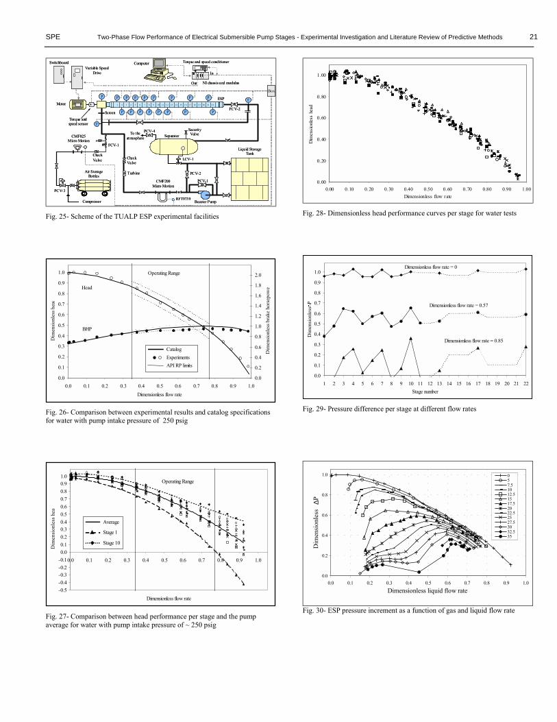
SPE Two-Phase Flow Performance of Electrical Submersible Pump Stages - Experimental Investigation and Literature Review of Predictive Methods 21

Booster Pump

Variable Speed Drive

Torque and speed sensor

Motor

Liquid Storage Tank

Separator

PCV-1CMF200Micro Motion

FCV-2

ESPP

T

TP

P

10

P P P P P P P

P P P P P P P

2 211 1 2 13 1 4 15 1 6 1 7 18 211 2 3 4 5 6 7 8 9

Compressor

Air Storage Bottles

FCV-1

1 9 20

CMF025Micro Motion

Torque and speed conditioner

NI chassis and modulus

Box

Check Valve

Turbine

Check Valve

Screen

Computer

In

Out

PCV-3

LCV-1

PCV-2

RFT9739

PCV-4To theatmosphere

SecurityValve

Switchboard

Booster Pump

Variable Speed Drive

Torque and speed sensor

Motor

Liquid Storage Tank

Separator

PCV-1CMF200Micro Motion

FCV-2

ESPP

T

TP

P

10

P P P P P P P

P P P P P P P

2 211 1 2 13 1 4 15 1 6 1 7 18 211 2 3 4 5 6 7 8 9

Compressor

Air Storage Bottles

FCV-1

1 9 20

CMF025Micro Motion

Torque and speed conditioner

NI chassis and modulus

Box

Check Valve

Turbine

Check Valve

Screen

Computer

In

Out

PCV-3

LCV-1

PCV-2

RFT9739

PCV-4To theatmosphere

SecurityValve

Switchboard

Fig. 25- Scheme of the TUALP ESP experimental facilities

0.0

0.1

0.2

0.3

0.4

0.5

0.6

0.7

0.8

0.9

1.0

0.0 0.1 0.2 0.3 0.4 0.5 0.6 0.7 0.8 0.9 1.0Dimensionless flow rate

Dim

ensio

nles

s hea

d

0.0

0.2

0.4

0.6

0.8

1.0

1.2

1.4

1.6

1.8

2.0D

imen

sionl

ess b

rake

hor

sepo

wer

Operating Range

API RP limits

CatalogExperiments

Head

BHP

Fig. 26- Comparison between experimental results and catalog specifications for water with pump intake pressure of 250 psig

-0.5-0.4-0.3-0.2-0.10.00.10.20.30.40.50.60.70.80.91.0

0.0 0.1 0.2 0.3 0.4 0.5 0.6 0.7 0.8 0.9 1.0

Dimensionless flow rate

Dim

ensi

onle

ss h

ea

Average

Stage 1

Stage 10

Operating Range

Fig. 27- Comparison between head performance per stage and the pump average for water with pump intake pressure of ~ 250 psig

0.00

0.20

0.40

0.60

0.80

1.00

0.00 0.10 0.20 0.30 0.40 0.50 0.60 0.70 0.80 0.90 1.00Dimensionless flow rate

Dim

ensio

nless

hea

d

Fig. 28- Dimensionless head performance curves per stage for water tests

0.0

0.1

0.2

0.3

0.4

0.5

0.6

0.7

0.8

0.9

1.0

1 2 3 4 5 6 7 8 9 10 11 12 13 14 15 16 17 18 19 20 21 22Stage number

Dim

ensio

nles

s P

Dimensionless flow rate = 0

Dimensionless flow rate = 0.57

Dimensionless flow rate = 0.85

Fig. 29- Pressure difference per stage at different flow rates

0.0

0.2

0.4

0.6

0.8

1.0

0.0 0.1 0.2 0.3 0.4 0.5 0.6 0.7 0.8 0.9 1.0Dimensionless liquid flow rate

Dim

ensi

onle

ss

∆P

057.51012.51517.52022.52527.53032.535

Fig. 30- ESP pressure increment as a function of gas and liquid flow rate

22 RUI PESSOA, RAGHAVAN BELTUR AND MAURICIO PRADO SPE

-0.6

-0.4

-0.2

0.0

0.2

0.4

0.6

0.8

1.0

0.00 0.20 0.40 0.60 0.80 1.00

Dimensionless liquid flow rate

Dim

ensio

nles

sP

-0.2

0.0

0.2

0.4

0.6

0.8

1.0

0.0 0.2 0.4 0.6 0.8 1.0

Dimensionless liquid flow rate

Dim

ensio

nles

s P

0.0

0.2

0.4

0.6

0.8

1.0

0.0 0.2 0.4 0.6 0.8 1.0Dimensionless liquid flow rate

Dim

ensi

onle

ss P

0.0

0.2

0.4

0.6

0.8

1.0

0.0 0.2 0.4 0.6 0.8 1.0Dimensionless liquid flow rate

Dim

ensio

nles

s P

Fig. 31- Pressure increment for stages #1 (a. upper left), #2 (b. upper right), #10 (c. lower left) and #22 (d. lower right) at different gas flow rates

0.0

0.2

0.4

0.6

0.8

1.0

0.0 0.1 0.2 0.3 0.4 0.5 0.6 0.7 0.8

Dimensionless liquid flow rate

Dim

ensio

nles

s P

-0.2

0.0

0.2

0.4

0.6

0.8

1.0

0.0 0.1 0.2 0.3 0.4 0.5 0.6 0.7 0.8

Dimensionless liquid flow rate

Dim

ensio

nles

s P -0.2

0.0

0.2

0.4

0.6

0.8

1.0

0.0 0.1 0.2 0.3 0.4 0.5 0.6 0.7 0.8

Dimensionless liquid flow rate

Dim

ensio

nles

s P

stage 1stage 2stage 3stage 4stage 5stage 6stage 7stage 8stage 9stage 10stage 13stage 17stage 22

Fig. 32- Pressure increment for all stages at 5 Mscf/d (a. upper left), 7.5 Mscf/d (b. lower left) and 15 Mscf/d (c. Right)

Fig. 33- ESP pressure increment as a function of gas and liquid flow rate - 3D view

Fig. 34- ESP pressure increment behavior � gas and liquid flow rates and free gas fraction effect

0.000.050.100.150.200.250.300.350.400.450.50

0.0 0.1 0.2 0.3 0.4 0.5 0.6 0.7 0.8 0.9

Dimensionless liquid flow rate

HPg

/ H

P5 7.510 12.515 17.520 22.525 27.530 32.535

Fig. 35- Gas to liquid hydraulic horsepower ratio for stage 3

0.0

0.2

0.4

0.6

0.8

1.0

1.2

0.0 0.2 0.4 0.6 0.8 1.0

Dimensionless liquid flow rate

Hyd

raul

ic ho

rsep

ower

(HP

0 57.5 1012.5 1517.5 2022.5 2527.5 3032.5 35

Fig. 36- Average hydraulic horsepower for the pump (isothermal gas compression)

SPE Two-Phase Flow Performance of Electrical Submersible Pump Stages - Experimental Investigation and Literature Review of Predictive Methods 23

0.00.10.20.30.40.50.60.70.80.91.0

0.0 0.2 0.4 0.6 0.8 1.0

Dimensionless liquid flow rate

Hyd

raul

ic ho

rsep

ower

(HP

Fig. 37- Total Hydraulic horsepower for stage 1 at different gas flow rates

0.0

0.2

0.4

0.6

0.8

1.0

1.2

1.4

1.6

1.8

2.0

0.0 0.1 0.2 0.3 0.4 0.5 0.6 0.7 0.8 0.9 1.0

Dimensionless liquid flow rate

Bra

ke h

orse

pow

er (H

P)

Water 5.0 MSCF/D 7.5 MSCF/D 10.0 MSCF/D 12.5 MSCF/D 15.0 MSCF/D 17.5 MSCF/D20.0 MSCF/D 22.5 MSCF/D 25.0 MSCF/D 27.5 MSCF/D 30.0 MSCF/D 32.5 MSCF/D 35.0 MSCF/D

Fig. 38- Average brake horsepower for the pump

0

10

20

30

40

50

60

70

0.0 0.1 0.2 0.3 0.4 0.5 0.6 0.7 0.8 0.9 1.0Dimensionless liquid flow rate

Eff

icie

ncy

(%)

Water 5.0 MSCF/D 7.5 MSCF/D 10.0 MSCF/D 12.5 MSCF/D 15.0 MSCF/D 17.5 MSCF/D20.0 MSCF/D 22.5 MSCF/D 25.0 MSCF/D 27.5 MSCF/D 30.0 MSCF/D 32.5 MSCF/D 35.0 MSCF/D

Fig. 39- Average efficiency for the pump (isothermal gas compression)