Série des Documents de Travail

n° 2014-48

A Long-Term Evaluation of the First Generation of the

French Urban Enterprise Zones

P.GIVORD 1 S.QUANTIN2 C.TREVIEN3

Les documents de travail ne reflètent pas la position du CREST et n'engagent que leurs auteurs. Working papers do not reflect the position of CREST but only the views of the authors.

1 CREST, INSEE.E-mail: Pauline.givord@insee.fr

2 INSEE.E-mail: simon.quantin@insee.fr

3 CREST,INSEE, SciencesPo.E-mail: corentin.trevien@insee.fr

A Long-Term Evaluation of the First Generation of the

French Urban Enterprise Zones ∗

Pauline Givord†

Simon Quantin‡

Corentin Trevien§

March 9, 2015

Abstract

This paper provides new empirical assessment on the long-term efficiency oflocally-targeted tax incentives in revitalizing distressed areas, and on the impact onlocal population. We focus on the first generation of the French “Enterprise Zone”initiative, implemented in 1997 in France. On the opposite to previous results ofsimilar program in France, we observe strong positive impact of EZ on economicactivity in the short-run, robust to several identification strategy. However, long-run estimates suggest that this program fails to impulse self-sustaining economicdevelopment. After five years, the early positive results are reduced as the increasein business locations is partially offset by more frequent business discontinuations.Besides, the small impact on resident employment and on local services suggests alack of accurate targeting.

Keywords: Enterprise Zones, Local Employment, Propensity Score Matching, Evalua-tion.JEL: C23, H71, R5

∗We thank participants of INSEE, Economic Department of Sciences Po and CREST seminars as wellas French Applied Microeconomics Conference, European Economic Association congress and EuropeanRegional Science Association congress. We thank more specifically Luc Behaghel, Didier Blanchet,Anthony Briant, Xavier D’Haulfœuille, Laurent Gobillon and Thierry Mayer for useful comments anddiscussions. Any opinions expressed in this paper are those of the author and not of any institution.†INSEE-CREST, pauline.givord@insee.fr‡INSEE, simon.quantin@insee.fr§INSEE-SciencesPo.-CREST, corentin.trevien@insee.fr

1 Introduction

The provision of locally-targeted tax credits and subsidies to kickstart sustainableeconomic development has become a widely used policy tool. Indeed, the first so-called“Enterprise Zone” programs were implemented in the UK in the 1980s, and others fol-lowed in several US states and elsewhere. In France, the EZ (”Zones Franches Urbaines”)program first came into existence in 1997. This program grants temporary but remark-ably generous tax incentives to small firms which choose to locate in economically dis-tressed areas. The rationale guiding policy makers when opting for an EZ program isquite simple: reductions in tax are meant to offset the numerous disadvantages associ-ated with deprived areas, such as the shortage of a skilled labor force, the lack of publicservices, a dearth of inputs, and poor market potential. The EZ initiative may stim-ulate local economic activity, by attracting firms that will employ the locally residentworkforce, and may “revitalize” these neighborhoods by improving the local amenities(health services, convenience stores...). The spinoff effects ought to include increasedlocal demand, and greater incentive for other new firms to choose the same locationbecause of agglomeration economies. Once this initial boost had been delivered, the EZinitiative was expected to terminate.

However, as stressed by Neumark and Simpson (2014) in a critical review of thealready large economic literature on place-based policies, the theoretical foundations ofthese policies have not been well established (see also Kline and Moretti 2014). As well,these programs may have potential adverse effects such as inducing firms to hire workerswho are already involved in work-based networks, instead of targeting local unemployedpeople for their hires; and they may have negative externalities on neighboring localitieswhich are often not much better off than the EZ itself. The variety of empirical evalu-ations of these policies, which mostly focus on their impact on employment, reflects theambiguity of the theoretical mechanisms. Although most evaluations find no significantincrease in employment (see for instance Bondonio and Greenbaum, 2007 or Neumarkand Kolko, 2010 for the US enterprise Zones, or Accetturo and de Blasio, 2011 for theItalian “Patti Territoriali”), a significant minority do (see for instance Ham, Swenson,Imrohoroglu, and Song 2011, Busso and Kline 2008). For France, several papers focuson the second wave of the EZ program, implemented in 2002. They obtain a significantbut small impact on firm locations and related employment (see for instance Givord,Rathelot, and Sillard, 2013 or Mayer, Mayneris, and Py, 2012). Still, the breadth ofthe empirical literature on place-based programs notwithstanding, many questions re-main unanswered. Neumark and Simpson (2014) identify a research agenda, suggestingseveral areas where evidence capable of guiding policy is still lacking. Investigating thelong-term effect of these programs is the first of them, as one of the main challenges ofplace-based policy is to generate self-sustaining economic gains. The other open ques-tions include: a more precise identification of “what the effects are” and who gains andwho loses from the policy-based question; and “isolating features of policies that makethem effective”.

1

This paper derives from this research agenda. More specifically, we focus on the firstwave of French EZ created in 1997, to evaluate whether this initiative was able to yieldlong-term economic activity. We try to assess whether the program has had a positiveimpact on the living conditions of the inhabitants of these disadvantaged neighborhoods.More specifically, while most previous related studies focus on overall firm employment,we analyze resident employment separately from non-resident employment. We alsofocus on firms engaged in providing local services, as one stated objective of the EZinitiative was to give the local population better access to the sort of “basic” services(physicians, convenience stores, independent retailers like bakers, and tradesmen likeplumbers...) that are more likely to suffer hardship from being located in distressedurban areas (small market potential in low-income neighborhoods, low accessibility fornon-local employees, high rates of criminality).

Interestingly, while we use similar geolocalized data and the same propensity scoremethod as previous empirical evaluations, which focused on the second wave of thisinitiative, the results we obtain for the first wave of the French EZ initiative are verydifferent from their findings. While Givord, Rathelot, and Sillard (2013) observe verylittle impact on the number of plants and employment, we observe on the contrary thatthe first EZ initiative caused these outcomes to respectively double and triple over afive-year period, compared to the baseline level that would have been achieved withouttax rebates. These surprising results are robust to an alternative identification strategyrelying on a regression discontinuity design method, for the 44 EZ included in the firstwave of the program were indeed selected (out of a previously compiled long list of 450deprived areas) by relying on a discontinuity rule (only the most populated areas wereselected).

Apart from this short-term comparison, our results, covering as they do a muchlonger period (twelve years) than previous studies, highlight the fact that the short-termassessment of the French EZ initiative may differ sharply from the medium and long-term ones. We observe that the number of firms newly located in EZ increases the firstyear, and stays at a high level for the next four years. But during this period, the paceof firm closures progressively grows and finally overtakes the pace of new firm locations.This suggests that firms that do choose to locate in an EZ may be non-economicallyviable ones, likely to fail when they are not subsidized anymore. Besides, firms arefree to relocate outside the EZ after the end of the program : the tax cuts are grantedto a given firm for only five years. Indeed, a significant part of the EZ effect flowsfrom firm relocations, suggesting the presence of a windfall effect. This result challengesthe intuition that an EZ can induce a change in the economic spatial equilibrium, bycreating a “virtuous circle.” And the fact of the matter is that, while the EZ initiativewas originally planned to be temporary, its lifespan has been prolonged repeatedly.

Concerning the situation of the inhabitants of these disadvantaged areas, our resultssuggest that the EZ initiative achieves its objectives, but only on a limited scale. This inturn suggests a lack of clear targeting of the EZ initiative. Overall, the employment leveldoes increase in the EZ thanks to tax cuts: it is 3 times higher than its counterfactual

2

level after five years, and a portion of the employees concerned do live in the munici-palities including the disadvantaged areas. However, while the EZ initiative explicitlyincludes a clause favoring local hiring, in practice the share of local residents employedin firms located in EZs tends to decrease over the period. As regards local amenities,we do observe a positive effect on location decisions by firms in the corresponding sector(trade, health or community services), as the number of these firms increases by 50%after ten years. But this figure is much smaller than the corresponding one for the “foot-loose” firms of the business services sector (office cleaning, security, IT services...). Thenumber of these firms who do operate locally and may easily leave the areas when taxbreaks end, increases by 300% after ten years thanks to the EZ initiative.

The paper is organized as follows. Section 2 presents the French EZ program, theEZ areas, and estimates of the magnitude of the financial incentives provided by theprogram. The data are briefly presented in the following Section. Identification issuesare discussed in Section 4. Section 5 displays the results and Section 6 concludes.

2 The French Enterprise Zones

2.1 Selection of the Enterprise Zones

Urban decay has become a main topic of French public debate since the 1980s. Arange of policies have been implemented in response to social and economic problemsexperienced in the deprived outskirts of France’s cities. Indeed, the so-called ”socialfracture” (”fracture sociale”) was an important theme of the 1995 presidential campaign,with the social and economic circumstances in deprived urban areas being identified asthe main causes. The ”stimulus for cities” law (”Pacte de relance de la ville”), passedin 1996 by the newly elected Government, aimed at addressing the issue of urban decayand reducing inequalities between urban neighborhoods.

This law resulted in the implementation of tax cuts for businesses located in thosedeprived areas. More precisely, this policy instituted a three-tier classification schemefor disadvantaged urban areas. The first tier is known as ZUS (”Deprived Urban Ar-eas”). They correspond to the 757 most deprived areas in France,1 according to variousindicators of socio-economic development (in particular, high concentrations of socialhousing and high unemployment rates). The second tier, the ZRU (”Urban RenewalAreas”), contains the most disadvantaged ZUS ranked by a global index of their socialand economic position. This index takes into account the unemployment rate, the pop-ulation size, the proportion of unskilled people, the proportion of young people and thepotential tax revenue (product of the tax base by the medium tax rate) of the city. Itcorresponds to the product of the four first indicators divided by the fifth one. 436 ZRUwere designated in 1996.2 Finally, the third tier is constituted by ZFU (”Urban En-

1717 in continental France and 40 ZUS in French overseas departments. 4.73 millions of people livedin ZUS according to 1990 census data.

2416 in continental France and 20 in French overseas departments in 1996.

3

terprise Zones”), hereafter EZ. These zones are chosen in a two-stage process: only themost populous ZRU are eligible, the official threshold being 10,000 inhabitants, and outof that set the most deprived ZRU, as defined by the same global rating, are designatedas Enterprise Zones. In 1997, during the first phase of this initiative, 44 areas receivedthe EZ designation, followed by an additional 41 in 2004 and 15 more in 2007.

Figure 1 illustrates, in the case of the Paris metropolitan region, the uneven localdistribution of the unemployment rate, as well as the location of some EZ. This region isthe wealthiest in France, but the unemployment rate varies markedly amongst municipal-ities. The inner northeast suburbs of Paris are a site of concentrated economic difficulty.This large sector apart, municipalities characterized by high rates of unemployment arespread throughout the region. The EZ are located in such economically distressed mu-nicipalities, but not always. This is explained by the fact that the unemployment rate insome neighborhoods (the relevant geographical level for EZ) may largely exceed the oneestimated at the municipality level. Besides, due to the political bargaining involved,hence the need to disperse targeted areas across France, the designation of EZ doesn’trely on a deterministic way on the index indicating the social and economic position.The upshot is that the EZ are uniformly spatially distributed across France, while urbandeprived areas are mostly concentrated in a limited number of municipalities.

2.2 Advantages granted by the EZ policy

Enterprise Zones offer remarkably generous incentives (deep tax cuts on property,labor and business taxes). They target only small firms (establishments with less than50 employees, with an additional condition on the volume of sales), whether located inthe area prior the introduction of EZ policy or not (see Table 1 and Appendix A fordetails). Full exemption is granted for a minimum of five years. In comparison to thetax relief available in EZ, the ZRU and ZUS designations provide much shallower taxcredits. The ZRU program provides limited tax cuts, for newly created firms only andover a shorter period (one or two years after startup, depending on the tax). Payrolltax exemption applies to all employees in EZ, while it remains limited to newly hiredemployees in ZRU. Finally, the ZUS program merely allows local authorities to exemptfirms from local business taxes, nor is this tax break mandatory.

The first generation EZ were implemented in 1997 and scheduled for five year. Asinitially planned, the policy ended in 2001: businesses had to locate in a Enterprise Zonebefore December 31 to benefit from the tax exemptions. However, the EZ policy wasreactivated in 2003 and has been kept alive continuously since then. New areas weredesignated successively in 2004 and 2007, for a total number of 100 EZ today.

The financial incentives depend on the actual financial burden for small firms, and onthe structure of their revenues and costs. To assess the actual generosity of this program,we simulate the benefit using individual databases that provide accurate information (seeAppendix B). According to these simulations, payroll tax exemptions account for thelargest share of tax reductions. In 1997, the median cut in payroll taxes associated

4

with EZ was 6,000 euros and this cut accounted for about 15% of the median wage bill(see Table B.1). This relative advantage was slightly reduced after the introduction ofnational payroll scheme changes in 2003 but EZ remain attractive. Under the schemeof payroll taxes in use since this date, the median gain for firms from being located inan EZ still accounts for about 12% of the median labor cost (with an amount of 4,500euros).

Eligible firms also benefit from a full exemption from corporate income tax, up to alimit that cannot exceed 20,000 euros per year. In practice, a closer look at real data sug-gests that this exemption is not as appealing as it may seem. Before the implementationof EZ, more than three quarters of small firms did not pay any corporate income tax.For those which did pay a strictly positive corporate income tax, the median amountpaid was 3,700 euros (see Table B.2).

3 Data

We exploit two exhaustive administrative datasets to gather rich information on firmdemography (number of plants) as well as employment (see details in the appendix C).

The French business register (SIRENE) follows all French firms and plants. Every1 January, it displays the location of each plant, its firm’s legal status, its industry andyear of creation. This register also tracks plant creations and relocations from 1 Januaryto 31 December each year. It thus enables us to specify whether a new plant location isan actual creation or a relocation of an existing plant. It also allows us to identify whenbusinesses cease activity. Above all, SIRENE locates precisely all plants in continentalFrance. Thus, we can accurately identify which plants have settled in an EZ and thosewhich have not, which is crucial as EZ do not correspond to administrative boundaries(see also Givord, Rathelot, and Sillard 2013). Indeed, using data even at the level ofthe smallest French administrative subdivision (the municipality, or commune) wouldhave yielded an underestimation of the impact of tax exemptions, because plants whichbenefit from EZ tax breaks would have been grouped with plants which do not.

The second dataset (DADS) is an exhaustive administrative employer-employee databasewith information on the workforce of plants. Employment can be measured in variousways at plant level: full-time equivalents over a year, number of employees at any pointof time or as of 1 January. We use this latter measure, which is consistent across yearsand consistent with the French business register. The DADS thus provides a measure oflocal employment, meaning employment in plants located in the area. Moreover, DADSallows us to split our employment measure into low-skilled, skilled and high-skilled em-ployment, and also into resident and non-resident employment.

These data allow us to probe the long-run effects of Enterprise Zones, as well astemporal delays or extenuations. SIRENE and DADS are available from 1995 to 2007.This means that we observe data at least 2 years before the introduction of the EZ tax

5

exemptions and up to 10 years after.

Finally, the 1990 Population Census allows us to measure socio-demographic variablesused for the designation of an area as an Enterprise Zone. For this evaluation, the datahave been aggregated at the three-tier classification levels presented in section 2: EZ,ZRU and ZUS.

4 Identification issue and empirical strategy

4.1 Identification issue and process of selection to EZ system

We restrict our estimation sample to the comparison set of non-beneficiary areas (i.e.the control group) to ZRU, which are areas most similar to EZ. Panel data allow us toeliminate the potential fixed effect specific to each area. More precisely, our main vari-ables of interest are (log-) outcome-level differentiated based on data from 1995, meaningtwo years prior to the introduction of the tax exemptions (the aim of using such a lag isto avoid capturing potential anticipation effects of the measure, for instance).Time-differentiation is not sufficient to accurately estimate the causal impact of the EZsystem. Indeed, the EZ were chosen from among ZRU suffering from multiple economichandicaps that may also have had an impact on the economic perspective. However, thetwo-step assignment process does provide us with an identification strategy.

First, the eligibility condition based on the size of the areas (in terms of inhabitantsestimated in the 1990 population census) ensures that non-EZ areas comparable to EZin terms of socio-economic development can be found. Indeed, almost all EZ have morethan 10,000 inhabitants (see Figure 2).3 This assumption is supported by descriptivestatistics on socio-economic characteristics (see Table 2). For each criterion (unemploy-ment rate, percentage of social housing, percentage of young people, foreign people andunskilled people in the area, and potential tax revenue in the municipality in 1996),average figures in small ZRU (meaning those populated by less than 10,000 inhabitants)appear close to the EZ; in some cases they are worse. For instance, the average unem-ployment rate is 22% in EZ while it is “only” 18% in big ZRU but 24% in small ZRU.The proportion of unskilled people is 43% in EZ, while it is 36% (respectively 46%) inbig (respectively small) ZRU.

Second, as we know and measure the characteristics used in the EZ designation, wecan accurately control for differences arising from this selection process. This suggests thechoice, common in this literature, of an estimation based on the propensity score method.However, we adapt the estimation to take into account the discontinuity introducedby the eligibility threshold. Moreover, this eligibility condition provides an alternativeidentification strategy based on regression discontinuity that we will use as a robustness

3With the exception of four areas: two very small zones that were merged to bigger EZs, and twoareas that are just below the threshold, with 9,538 and 9,927 inhabitants, respectively.

6

check of our results.

4.2 Estimator based on the propensity score

4.2.1 Subclassification on the propensity score and Regression

In practice, we compare the evolution of outcomes in EZ by using areas that do notbenefit from the EZ initiative, but are similar in terms of socio-economic characteristics.More specifically, our main assumption is the standard “conditional independence as-sumption” (CIA) (or unconfoundedness assumption) which states that, in the absence ofthe policy, no difference would have been observed in the evolution of outcomes in zoneswith comparable observable characteristics. As we use outcomes in temporal differences,this method is often named “conditional difference in differences”.

As shown by Rosenbaum and Rubin (1983a), if the CIA holds for observables X, italso holds for the propensity score P (Ti = 1|X) (i.e. the probability of an area beingdesignated as an EZ, conditional on observables). In practice, we use as control variablesthe indicators formally used for the designation of EZ, but also other indicators that mayhave an impact on both designation and economic outcomes, namely the proportion offoreigners and executives in the area, as well as the proportion of stable households andthe amount of social housing.

However, as our sample size is small, simple propensity-score matching might lead usto compare units with different observable characteristics (as areas with close propensityscores may still have different observable characteristics). To address this issue, we adopta strategy that combines regression and propensity score methods for the final estimateof the impact of the EZ. More precisely, we define four strata corresponding to the levelof the propensity score, and perform a linear regression using observable covariates X.As discussed by Imbens and Wooldridge (2009), the linear regression (originally sug-gested by Rosenbaum and Rubin 1983b) helps to eliminate potential remaining bias andto improve precision. Within each block, the propensity score does not vary much, andcovariate distributions are on average similar between both groups. This insures thatthe regression function will not extrapolate, perhaps erroneously, into regions outside thedata range. The estimate of average treatment effect on the treated (ATT) correspondsto the weighted average of these local estimates.

Formally, and using notation posited by Imbens and Wooldridge (2009), we performthe linear regression in each stratum j:

∆1995log(Yit) = Xiβj + δjTi + uij (1)

If we denote J the number of strata (four in our estimates), the final estimate of theimpact of the tax subsidies on the EZ δATT corresponds to:

7

δATT =

J∑j=1

NjEZ

NEZδj

and an estimate for its variance is:

V =J∑

j=1

(NjEZ

NEZ

)2

Vj

where (Vj)j=1,...,J corresponds to the estimated variances of (δj)j=1,...,J (assuming thatthe residuals for different strata are independently distributed, which is a standard as-sumption in this kind of method) and NjEZ and NEZ respectively denote the numberof EZ in strata j and in the whole sample. We introduce the number of inhabitantsof the area as an additional covariate in (1), as an informal test of the assumption ofconditional independence of outcome and size. It is never significant.

4.2.2 Propensity score estimation

Because of the eligibility condition based on the number of inhabitants in the area,we adapt the estimation of the propensity score to this specific setting. This size condi-tion reinforces the credibility of our identifying assumption (as it ensures that we havecontrol with close characteristics), but it can impact the estimation of the propensityscore. Indeed, it leads to a censoring for the observed status (EZ or not) of an area. Ifsome observable characteristics used for the score are correlated with the size of the area(or, to put it differently, if the distribution of observables is not the same in small andlarge areas as shown in Table 2 for instance), a “naive” estimation of the propensity scoremay lead to biased estimates of the correlation between observed covariates and the score.

Formally, we can assume that the fact of being selected as an EZ, Ti, depends on co-variates X, but an area is selected as an EZ if Ti = 1 and Si > S. As we wish to evaluatethe impact of being selected as an EZ, we are interested in estimating the propensity scoreP (Ti = 1, Si > S|X), which may be decomposed as P (Ti = 1|Xi, Si > S)P (Si > S|X).Under mild assumptions,4 we can estimate both components separately.

In practice, this means that we estimate as a function of the covariates both the prob-ability of being an EZ (restricting the sample to areas with more than 10,000 inhabitants)and the fact of having more than 10,000 inhabitants. The second estimation has no causalinterpretation, but corrects for misspecification due to differences in the distributions ofthe covariates in large and small areas. In both cases, we rely on logistic specifications.

4Meaning that in the absence of this eligibility condition, the fact of being EZ Ti is independentof being a “big” area Di conditional on the characteristics X, where the dummy Di = 1Si>S indicateswhether the size is higher than 10,000 inhabitants or not. Indeed one may easily show that the likelihoodof the observations (Di, TiDi) is separable in both components.

8

These estimations are provided in Table 3. The first column displays the estimated im-pacts, for a ZRU with more than 10,000 inhabitants of various socio-economic criteria,on the probability to be included in the EZ program (i.e. P (Ti = 1|Xi, Si > S)). Asexpected, this probability is an increasing function of the unemployment rate and theproportion of young and unskilled people, and a decreasing function of the potential taxrevenue of the municipality, as it corresponds to the criteria in the selection process.EZ are also characterized by a higher proportion of social housing and foreigners, anda lower proportion of executives and stable households. We now turn to the estimatesof the impact of the same range of criteria on the probability for a ZRU to have morethan 10,000 inhabitants (i.e. P (Si > S|X)); the results are displayed in the second col-umn. They suggest that the distribution of these variables (in particular, proportion ofexecutives, potential tax revenue and proportion of unskilled people) are not the samein small and in large ZRUs.

Finally, the estimated propensity score for one ZRU corresponds to the product ofthe two predicted probabilities, given the observed covariates of this area. Figure 3 showsthe density of the propensity score for both the treated and control groups. The treatedgroup contains 45 areas, and the control group contains 331 areas. As expected, weobserve two distinct modes, meaning that the distributions of the covariates are differentin both groups. However, the common support is large, meaning that comparable areasmay be found for most EZ.

4.3 Regression Discontinuity Design

We also use the eligibility threshold to propose an alternative strategy. Indeed, theprobability that a given ZRU will be chosen to benefit from the EZ program increasessharply at the 10,000 inhabitants threshold (see Figure D.1). The design is only “fuzzy,”as the EZ selection process is not a deterministic function of population size : numerouslarge ZRU have not become EZ, and a few small ZRU have become EZ. Our settingis very similar to that of Battistin and Rettore (2008), where endogenous selection oc-curred amongst a pool of eligible units. One threat to the validity of this approach ariseswhen the selection variable can be manipulated by economic agents in order to be on the“favorable” side of the threshold. In our case, this selection variable was measured in the1990 population census, meaning five years before the selection process, so manipulationappears very unlikely.

The fuzzy estimator can be obtained using a two-stage-least-square on the linearregression (for details see Imbens and Lemieux 2008), restricting the estimation sampleto units in a small neighborhood to the left and right of a threshold S, defined with abandwidth h by [S − h;S + h].

Formally, we estimate

∆1995log(Yit) = α+ δTi + β(Si − S)1Si>S + γ(S − Si)1Si<S + γXi + ui (2)

9

by two-stage least squares using the indicator 1Si>S as an excluded instrument.

A common tradeoff has to be made between increasing precision using a large band-width at the risk of using non-comparable units, and a small bandwidth that shrinks theestimation sample. In our case the tradeoff is constrained by the initial small samplesize : for instance considering the rather narrow window [9,000;11,000] inhabitants leftus with only 34 areas (including 5 EZ) that compromise statistical analysis. We havetested several sizes of the window around the threshold and have verified that only theprecision is altered by this choice. As is commonly done, we correct for potential de-pendency in the selection variable by a linear specification. Because of the small samplesize, it appears difficult to control for more complex dependence of outcomes on sizeareas using a polynomial specification of higher order. For the same reason, it is notpossible to include variables used in the selection process of EZ, in contrast to a moreflexible method such as the propensity score method. For this reason, and also becauseit makes our results more directly comparable to the results obtained by previous studiesthat evaluate the (second wave of) the EZ initiatives, we thus keep the propensity scorematching method as our main specification.

5 Results

5.1 Short-term effects

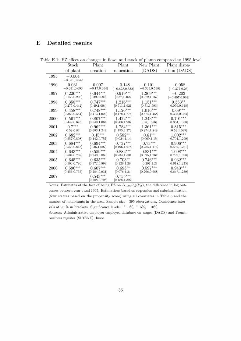
According to our results, Enterprise Zones have a strong impact on economic ac-tivity in targeted areas. Figure 4 displays the cumulative impact of the EZ programover time on number of plants and (salaried) employment (detailed results are presentedTable E.1 and Table E.2 in Appendix E). Tax exemptions result in a steady rise in thenumber of firms over the first five years. In 2001, the estimate of the impact of EZson the time-differentiated log number of plants located in Enterprise Zones is 0.7. Thismeans that the level reached in 2001 is e0.7 ≈ 2 times higher than the level that wouldhave prevailed without the policy. The estimated impact of EZs on salaried employmentis similar. From 2001, the number of salaried employees in EZ firms is 3 times higherthan its counterfactual level, according to our estimates. More concretely, a back-of-the-envelope estimate derived from our results suggests that the whole program wouldhave resulted during the first five years in the location of around 11,000 firms employing50,500 workers. 5 It is worth stressing that this effect strongly exceeds the findings ofprevious studies that evaluate the second-generation of the French Enterprise Zones (seeRathelot and Sillard 2008, Givord, Rathelot, and Sillard 2013). We discuss this point insection 6.As illustrated by Figures 4 and 5, our estimates also confirm that prior to the imple-mentation of the EZ program, the trend of economic activity was similar in future EZand in those zones used as a control group. Indeed, when applying the same estimationmethod to periods before the introduction of the EZ initiative (corresponding a“placebo”

5The impact of the EZ in the outcome in level corresponds to (1 − e−δt)Yi,t.

10

or “falsification” test), we cannot reject the null hypothesis of a null impact of the EZbefore the implementation of tax exemptions in 1997 (see precise estimates in Tables E.1to E.3 in Appendix D).

5.2 Long-term effects

Despite a promising start, several points cast doubt on the ability of the EZ programto impart a long-lasting momentum to economic activity. First, the impact appears tostabilize for both employment and firm location after 2001. This can be explained bythe fact that in-zone business locations are now canceled out by relocations outside theEZ, and business closures. Between 1997 and 2001, EZ had a notably higher impact onthe creation than on the shutdown of companies with salaried employees. From 2002,the two levels are no longer significantly different (see left panel in Figure 5 and TableE.1 in Appendix E). Interestingly, this realignment coincides with the termination of theprogram for the firms which entered it in 1997.

Besides, an increasing part of business location is due to relocation. The EZ impactgrows between 1997 and 2001, which are respectively the first year out and the fifthyear out from the policy implementation. This trend is greater for relocations than foractual creations. More precisely, the estimated impact with respect to plant relocationrises from 0.9 in 1997 to 1.8 in 2001 whereas it only increases from 0.6 to 1 for realcreations (see right panel in Figure 5 and Table E.1). To put it another way, in 2001 thenumber of firm relocations in EZ was 6 times higher than the level that would have pre-vailed without tax exemptions, while the number of true business creations was 2.7 timeshigher than its counterfactual level. Firm creations are still predominant among firm lo-cations (at its highest, the share of relocations is 35% in 2001 while it was 19% in 1995).6

Furthermore, whereas both newly located and existing plants benefit from tax ex-emptions, the EZ initiative has no impact on employment in existing plants (see TableE.2 in Appendix E). The higher level of employment (compared to the level that wouldhave prevailed in the absence of the EZ policy) appears to be solely due to plants estab-lished in EZ after 1995.

Finally, the number of plant locations, and especially relocations, increases sharply inEZ in 2001 but this impact declines in the subsequent year. This suggests that firms doanticipate the end of tax exemptions scheduled for 2001, the terminal date for the policywhen it was first announced. Businesses were required to locate in a EZ before December31, 2001 to benefit from tax exemptions. The return of the conservative party to powerin 2002 led to the reactivation of the EZ program after 2003 and firm creation almostrecovered to the initial level. This temporal profile suggests that EZ would not havecreated economic momentum in targeted areas that outlives the (costly) tax incentives.

6In 1995, 35 firms were created and 8 firms were relocated per EZ on average. Using our estimates for1997 (resp. 2001), we find that 74 (resp. 92) firms were created and 26 (resp. 48) firms were relocatedper EZ.

11

5.3 Impact on EZ residents

The original purpose of EZ was to contribute to urban renewal: the rise in economicactivity of firms was viewed as a way to improve the situations of local residents. Con-cerning this primary objective, our estimates suggest that the EZ program suffers froma lack of accurate targeting. Indeed, low priority outcomes are much more affected bythe EZ program than the hiring of residents and the development of local services.

Our data allow us to distinguish between resident employees (i.e. employees wholive in the municipality surrounding the EZ and who work in the EZ) with non-residentones. Indeed, local employment may increase both because more residents are hired,and also because of the hiring of commuters who live further afield. We observe thatresident employment does increase at a steady pace between 1997 and 2002 thanks tothe EZ initiative (see Table E.3 in Appendix E). However, this pace is slower thanthe one observed for non-resident employment. Thus, the share of resident employmentgoes down from 43% in 1995 before the program to 35% ten years later (estimates on thecausal impact of EZ on this rate are never significant at the usual level). The finding is inline with Gobillon, Magnac, and Selod (2012) who focus on the Paris metropolitan regionspecifically, and show that the EZ initiative has only a small and non-persistent effecton the unemployment rates of people living in the cities targeted by the EZ program.However, resident employment can be defined at a municipality level, as the place ofresidence of workers is not as precisely known as firm location. The impact of EZ onresident inhabitants may be consequently even smaller, as we include employees who donot live in the EZ.

Additionally, we decompose the impact of EZ on local employment by skill (see TableE.2). As low-skilled residents are over-represented in EZ and low-paid workers benefitfrom higher subsidies, a positive effect on low-skilled workers could be counted as anachievement of the EZ program. We observe that the program does have a positiveimpact on unskilled workers: after five years, our estimates reveal that the quantity ofunskilled employment in the areas is up to 3.2 times the level we should have expectedin the absence of the policy. However, these figures are not significantly different fromthose observed for skilled employment and high skilled employment. Interestingly, wefind a positive gap when comparing point estimates for low skilled and higher skilledemployment after 2002, that is to say, after the tax cuts were made conditional on localhirings. However, these differences are never statistically significant.

Finally, we break down results at the industry level, in order to evaluate whether ornot the EZ program helps to improve local services. Policy makers originally intendedto support local amenities, for instance small retail shops such as bakeries, and profes-sional services such as physicians. These correspond to the industrial sectors definedrespectively as ”trade” and “health, education and community services.” According toour results, the EZ initiative has a positive impact on both sectors (see Table E.4).However, the impact is smaller than the overall effect estimated. Indeed the number oftrade plants is 1.5 time higher than its counterfactual, whereas the overall effect estimatesuggests that the number of plants should have doubled thanks to the EZ program. As

12

well, a closer look suggests that the industrial sector most responsive to tax breaks isbusiness services. The impact of EZ is impressive here, as the estimated impact for thenumber of business service plants in the area peaks at 1.5 in 2001, meaning that theobserved level is 4.6 times higher than the counterfactual level. These plants correspondfor instance to IT services or office cleaning services, meaning companies whose activitiesare not necessarily carried out in the neighborhood, but whose legal address can easilybe located within the EZ. Such companies may also relocate easily when they no longerbenefit from tax exemptions.

5.4 Regression discontinuities design results and other robustness checks

We perform several robustness checks. First, as described earlier, we use an alterna-tive empirical strategy using RDD estimates that yield similar results. Second, we checkthat our control group provides an accurate counterfactual of a situation without localtaxes.

As discussed above in section 4, the selection process for EZ also suggests adoptinga fuzzy regression discontinuity design approach. Indeed, Figures D.2 and D.3 suggest adiscontinuous jump in the number of plants and the employment growth rate at aroundthe 10,000 inhabitants threshold. Table 4 provides estimates for the number of plants7

using the fuzzy RDD. The first column corresponds to the method based on propensityscore and subclassification, the results of which have already been discussed. The nexttwo columns both correspond to fuzzy RDD estimates. The first one, column (2), is basedon a regression on the whole sample correcting for dependence on size, corresponding tomodel (2). Column (3) is a two-stage least squares regression using a smaller windowaround the threshold.

The main conclusions remain unchanged. Using RDD estimates leads to the con-clusion that there was a non-significant impact of the EZ program for the first two tothree years, but the effect is similar and even higher in magnitude subsequently. Forinstance, in the fifth year after the implementation of the EZ program, its estimatedimpact on the growth in the number of plants ranges from 0.82 using RDD estimates(using a bandwidth of 3, 000 inhabitants, column (3)) to 0.91 (whole sample of 395 areas,controlling for size effect by a linear specification, column (2)), while it is 0.70 in ourmain estimations relying on the propensity score method. However, running such RDDestimates entails a loss of precision; this is partly due to the small sample size, as thesample size is limited to 103 areas with 12 EZ when restricting to a close bandwidth.

Finally, we check whether using ZRU as a control group does not lead to underesti-mating the impact of the EZ policy. The counterfactual situation we want to measureis a total absence of any tax exemptions. However, as firms located in this type of areado benefit from some (limited) tax exemptions, our results may underestimate the total

7For the sake of clarity, we present the estimates only for the stock of plants, but similar conclusionsare obtained for all outcomes. Results available upon request.

13

effect of EZs on economic activity, if the ZRU exemptions also have a positive impact.We thus estimate the impact of the ZRU program, applying the same methodology as forEZs. ZRUs are now considered as the treated group. We use disadvantaged urban areasthat do not benefit from tax breaks as a control group (i.e. ZUS, the first tier of Frenchurban policy, see section 2). According to our estimates, the tax exemptions providedby the ZRU program are inefficient at fostering economic activity (Table 4, column (4)).The evolutions of the stock of plants in ZRUs are never significantly different from thecase in ZUS over the whole 12-year period.8 The ZRU program thus has no significantimpact on economic activity, and we may be confident that our results do not under-estimate the impact of the EZ initiative. Indeed, compared to EZ, ZRU provide muchless generous tax breaks to firms, which moreover apply only to new firms (corporate andlocal business taxes) or new hires (payroll tax). Recent studies suggest that this specifictax scheme is less likely to attract firms. Duranton, Gobillon, and Overman (2010) findno impact of local taxation on non-residential property, on entry by English manufactur-ing establishments, and Rathelot and Sillard (2008) find significant but negligible impactfor French firms.

6 Discussion and conclusion

All in all, our results provide new evidence on the efficiency of the place-based pro-gram. The overall assessments are mixed, however. To the question “can such a programattract firms into disadvantaged areas,” the answer is clearly yes. French firms appearto be strongly reactive to tax breaks proposed by the EZ initiative. The change in stockof firms and local employment are impressive. Five years out from the introductionof the policy, the number of firms doubles compared to the level that would have pre-vailed without the tax exemptions. On the resident population, the consequences arealso positive if not as impressive. We observe a sharp increase in resident and unskilledemployment, as well as a clear but weaker rise in industries that provide local services.

However, analysis of the long term impacts mitigates these positive results. Indeed,the initial goal of the EZ policy was not to subsidize local economies endlessly. The firstfinancial impulse was expected to create self-sustaining economic activity, and was thusplanned to be temporary. Gauged in this light, the EZ initiative is less successful. Afterthe first five-year period of tax exemptions, the flow of new firms, while still steady,does not lead to an increase in employment: the reason is a higher firm closure rate (orrelocation of these firms outsize the areas). In other words, once firms cease to benefitfrom the tax rebates, they appear to be replaced by new firms which enter the program

8We observe a small impact on employment in 2005 and 2006, and on firm creations in 2007 (theresults are not reported here). This may reflect the fact that some ZRU became EZ in 2004 and 2007.Givord, Rathelot, and Sillard (2013) exhibit a significant impact (but much smaller than for the firstwave) of the policy on employment and business demography. As our control group includes some treatedareas, it might be “contaminated”: our main results could have been underestimated for the very end ofthe period. We have checked that we obtain similar conclusions when excluding areas selected for thesecond and third waves of Enterprise Zones from the control group (the results not reported here).

14

for the first time and can thus benefit from full tax exemption. Indeed, the program waseventually restarted in 2003, meaning that the stabilization in employment level and firmstock observed since this date has been achieved at substantial cost. The brief attempt tohalt the program in 2002 results in a significant decrease of new firm location for this year,highlighting the fact that the economic attractiveness of EZ remains largely dependenton tax rebates. Besides, as already noted by previous research on the French EZ, a largepart of the inflow of new firms is due to relocation. Subventions do not create genuinenew economic activity, and may have negative externalities on the not-so-advantagedneighborhoods close to the EZs, as observed by Givord, Rathelot, and Sillard (2013).Another drawback of the program may lie in its lack of clear targeting. The programhas certainly achieved one of its main objectives, that of increasing resident employmentand revitalizing the neighborhoods. But the impact appears relatively modest comparedto the overall cost of the program (estimated at 300 million euros in 2001 according toan official report by the French Parliament). Besides, Gregoir and Maury (2012) forinstance observe a negative impact on house prices in some French EZs of the secondwave, which they interpret as a negative signaling effect of EZ status on the population.

Many questions still remain open, about why and where the EZ work. The optimalsettings of such a place-based policy need to be evaluated, for EZ programs may proposea wide range of services, tax rebates and subsidies on certain inputs. Recent papersemphasize strong discrepancies linked to the variety of tax cuts (Lynch and Zax 2008),the services provided (Bondonio and Greenbaum 2007), the manner in which the zone ismanaged (Neumark and Kolko 2010), or the industrial sector in which firm is operating(Hanson and Rohlin 2011, Burnes, Neumark, and White 2012). For France, Briant,Lafourcade, and Schmutz (2012) highlight the importance of geographic context in thesuccess of the second wave of EZ.

The mixed success of French place-based policy also raises some questions. In theshort run, the impact of the first wave of the EZ was much higher than that obtainedin the second wave by Givord, Rathelot, and Sillard (2013) with similar data and closeidentification strategy (see also Mayer, Mayneris, and Py 2012). Several explanationscan be adduced to explain the apparent decline in the attractiveness of EZ. First, a largeprogram of payroll tax cuts has been implemented on a national scale and has reducedthe tax gap between EZs and the rest of the country. Second, after 2003 the subsidieswere more strictly contingent on hiring local workers. This so-called local employmentstipulation (“clause d’emploi local” in French) was already in effect between 1997 and2001, but there is evidence to suggest that it was not strictly enforced (see AppendixA). Real or supposed difficulties in hiring adequately skilled workers from among thepopulation of the area may have discouraged new firms from locating there.9 Finally,there are grounds for thinking that the number of plants that choose to relocate withinan EZ is bounded, either because of limited space, or because of a competition with the

9In 2008, according to a qualitative survey in the EZs, companies in these zones declare majordifficulties in hiring employees inside the area (and minor difficulties in hiring outside the area), asreported in Givord, Rathelot, and Sillard (2013).

15

second wave of EZ to attract plants that are likely to locate in deprived urban areas. Amore complete analysis of these issues in the future may supply useful elements aboutthe optimal settings of such a place-based policy.

16

References

Accetturo, A., and G. de Blasio (2011): “Policies for local development: an evalua-tion of Italy’s &quot;Patti Territoriali&quot;,” Temi di discussione (Economic workingpapers) 789, Bank of Italy, Economic Research and International Relations Area.

Battistin, E., and E. Rettore (2008): “Ineligibles and eligible non-participants as adouble comparison group in regression-discontinuity designs,” Journal of Economet-rics, 142(2), 715–730.

Bondonio, D., and R. T. Greenbaum (2007): “Do Local Taxes Incentives AffectEconomic Growth? What Mean Impacts Miss in the Analysis of Enterprise ZonesPolicies,” Regional Science and Urban Economics, 37, 121–136.

Briant, A., M. Lafourcade, and B. Schmutz (2012): “Can Tax Breaks Beat Geog-raphy? Lessons from the French Enterprise Zone Experience,” PSE Working Papershalshs-00695225, HAL.

Burnes, D., D. Neumark, and M. J. White (2012): “Fiscal Zoning, Sales Taxes, andEmployment: Do Higher Sales Taxes Lead to More Jobs in Retailing and Fewer Jobsin Manufacturing?,” IZA Discussion Papers 6383, Institute for the Study of Labor(IZA).

Busso, M., and P. Kline (2008): “Do Local Economic Development Programs Work?Evidence from the Federal Empowerment Zone Program,” Cowles Foundation Discus-sion Paper 1638.

Duranton, G., L. Gobillon, and H. G. Overman (2010): “Assessing the Effectsof Local Taxation using Microgeographic Data,” Working Papers 2010-47, Centre deRecherche en Economie et Statistique.

Givord, P., R. Rathelot, and P. Sillard (2013): “Place-based tax exemptionsand displacement effects: An evaluation of the Zones Franches Urbaines program,”Regional Science and Urban Economics, 43(1), 151–163.

Gobillon, L., T. Magnac, and H. Selod (2012): “Do unemployed workers benefitfrom enterprise zones? The French experience,” Journal of Public Economics, 96(9-10), 881–892.

Gregoir, S., and T.-P. Maury (2012): “Quel a ete l’effet de l’instauration de ZonesFranches Urbaines sur les marches immobiliers locaux ? Le cas de la Seine-Saint-Denis.,” Position paper, EDHEC.

Ham, J. C., C. Swenson, A. Imrohoroglu, and H. Song (2011): “Governmentprograms can improve local labor markets: Evidence from State Enterprise Zones,Federal Empowerment Zones and Federal Enterprise Community,” Journal of PublicEconomics, 95(7), 779–797.

17

Hanson, A., and S. Rohlin (2011): “The Effect of Location-Based Tax Incentiveson Establishment Location and Employment across Industry Sectors,”Public FinanceReview, 39(2), 195–225.

Imbens, G. W., and T. Lemieux (2008): “Regression discontinuity designs: A guideto practice,” Journal of Econometrics, 142(2), 615–635.

Imbens, G. W., and J. M. Wooldridge (2009): “Recent Developments in the Econo-metrics of Program Evaluation,” Journal of Economic Literature, 47(1), 5–86.

Kline, P., and E. Moretti (2014): “People, Places, and Public Policy: Some SimpleWelfare Economics of Local Economic Development Programs,” Annual Review ofEconomics, 6(1), 629–662.

Lynch, D., and J. Zax (2008): “Incidence and substitution in Enterprise Zone Pro-grams: The case of Colorado,” mimeo.

Mayer, T., F. Mayneris, and L. Py (2012): “The Impact of Urban Enterprise Zoneson Establishments’ Location Decisions: Evidence from French ZFUs,” CEPR Discus-sion Papers 9074, C.E.P.R. Discussion Papers.

Neumark, D., and J. Kolko (2010): “Do enterprise zones create jobs? Evidence fromCalifornia’s enterprise zone program,” Journal of Urban Economics, 68(1), 1–19.

Neumark, D., and H. Simpson (2014): “Place-Based Policies,” NBER Working Papers20049, National Bureau of Economic Research, Inc.

Rathelot, R., and P. Sillard (2008): “The Importance of Local Corporate Taxes inBusiness Location Decisions: Evidence From French Micro Data,”Economic Journal,118(527), 499–514.

Rosenbaum, P., and D. Rubin (1983a): “The Central Role of the Propensity Score inObservational Studies for Causal Effects,” Biometrika, 70, 41–55.

Rosenbaum, P. R., and D. B. Rubin (1983b): “Assessing Sensitivity to an UnobservedBinary Covariate in an Observational Study with Binary Outcome,” Journal of theRoyal Statistical Society. Series B (Methodological), 45(2), pp. 212–218.

18

●

●

●

●

●

●

●

●

●●●

●

●●

●

●

●

●

●●

●●

●●●

●

●● ●

●

●●

●●

●● ●

●

●

●●

● ●●●

●●

●

●●●

●●

●

●

●

●

● ●●

●●

●●●

●

●

EZZRUUnemployment rate<7.5%7.5%−10%7.5%−12.5%>12.5%

Figure 1: EZ location and unemployment rate in 1990 in the Paris metropolitan region.

0 10000 20000 30000 40000 50000

0

10

20

30

40

50 All ZRUEnterprise Zones

Figure 2: Distribution of EZs and ZRUs according to the number of inhabitants.

19

0

1

2

3

4

5

6

ZRUEnterprise Zones

Figure 3: Score density for the treated and control groups

1995 1996 1997 1998 1999 2000 2001 2002 2003 2004 2005 2006

0.0

0.2

0.4

0.6

0.8

1995 1996 1997 1998 1999 2000 2001 2002 2003 2004 2005 2006

0.0

0.5

1.0

Figure 4: Impact of EZs on the (log) stock of plants and (log) employment.

20

1996 1997 1998 1999 2000 2001 2002 2003 2004 2005 2006

−0.5

0.0

0.5

1.0

1.5

Plant locationPlant closure

1996 1997 1998 1999 2000 2001 2002 2003 2004 2005 2006 2007

−0.5

0.0

0.5

1.0

1.5

2.0

CreationRelocation

Figure 5: Impact of EZs on the (log) number of plant location and closure (left panel)and plant relocations and creations (right panel).

21

Table 1: French Enterprise Zone Tax Cuts

ZRU (1996-2004) ZFU (1996-2001)

Payroll tax exemptions

Plant eligibility with up to 50 employees

Employee eligibility new hires all employeesopen-ended contracts

fixed-term employment contract of more 12 months

Exemption fraction of salary ≤ 1.5 times the minimum wage

Duration 1 year 5 years

Corporate income tax exemptions

Eligibility newly created all (created, existing, relocating)(only in manufacturing, trade or craft in-dustry)

Exemption 100 % the first 2 years, and decreasing thenext 3 years

100 % during 5 years

Local business tax exemptions

Eligibility newly created all (created, existing, relocating)with up to 150 employees with up to 50 employees

Exemption 100 % during 2 years 100 % during 5 years

Local property tax exemption

Eligibility None all (created, existing, relocating)

Exemption 100 % during 5 years

Source: Legislative texts (Journal officiel, 1995).

22

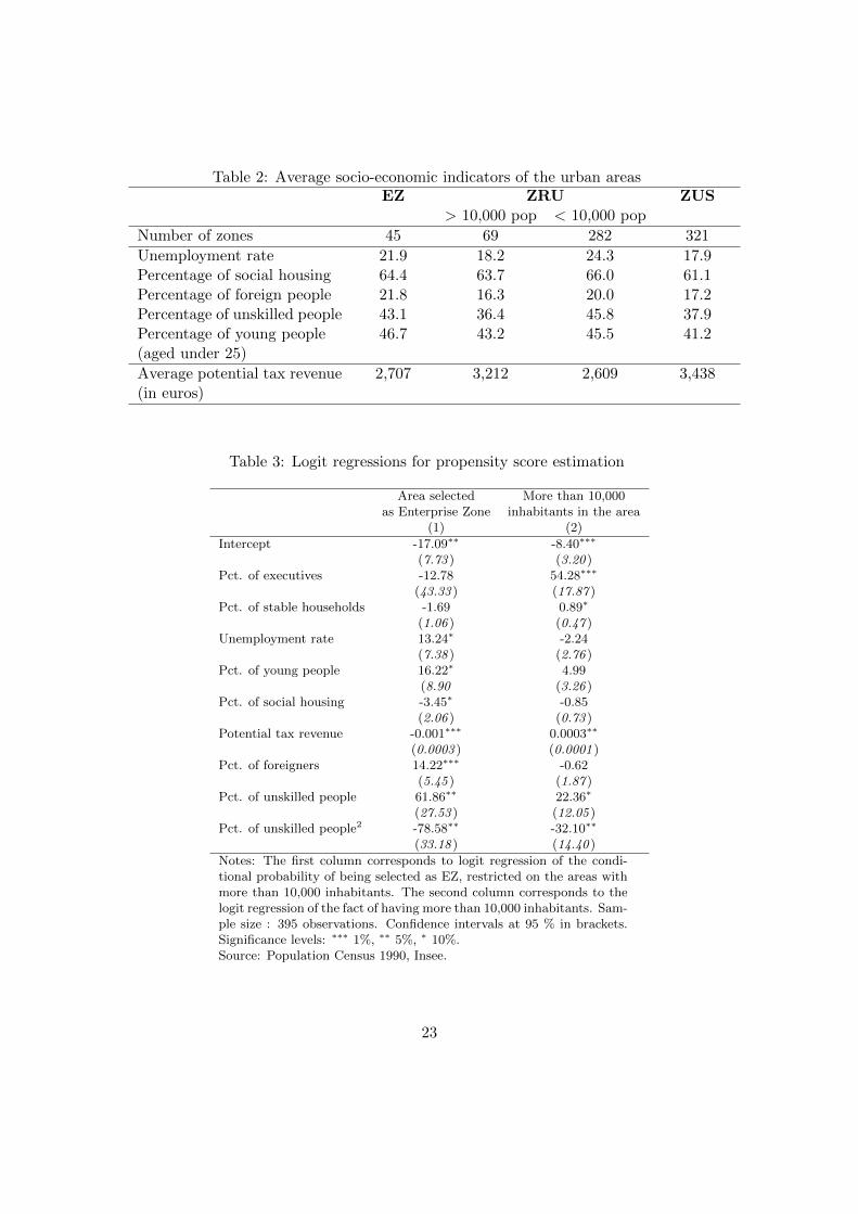
Table 2: Average socio-economic indicators of the urban areasEZ ZRU ZUS

> 10,000 pop < 10,000 pop

Number of zones 45 69 282 321

Unemployment rate 21.9 18.2 24.3 17.9Percentage of social housing 64.4 63.7 66.0 61.1Percentage of foreign people 21.8 16.3 20.0 17.2Percentage of unskilled people 43.1 36.4 45.8 37.9Percentage of young people 46.7 43.2 45.5 41.2(aged under 25)

Average potential tax revenue(in euros)

2,707 3,212 2,609 3,438

Table 3: Logit regressions for propensity score estimation

Area selected More than 10,000as Enterprise Zone inhabitants in the area

(1) (2)

Intercept -17.09∗∗ -8.40∗∗∗

(7.73 ) (3.20 )Pct. of executives -12.78 54.28∗∗∗

(43.33 ) (17.87 )Pct. of stable households -1.69 0.89∗

(1.06 ) (0.47 )Unemployment rate 13.24∗ -2.24

(7.38 ) (2.76 )Pct. of young people 16.22∗ 4.99

(8.90 (3.26 )Pct. of social housing -3.45∗ -0.85

(2.06 ) (0.73 )Potential tax revenue -0.001∗∗∗ 0.0003∗∗

(0.0003 ) (0.0001 )Pct. of foreigners 14.22∗∗∗ -0.62

(5.45 ) (1.87 )Pct. of unskilled people 61.86∗∗ 22.36∗

(27.53 ) (12.05 )Pct. of unskilled people2 -78.58∗∗ -32.10∗∗

(33.18 ) (14.40 )

Notes: The first column corresponds to logit regression of the condi-tional probability of being selected as EZ, restricted on the areas withmore than 10,000 inhabitants. The second column corresponds to thelogit regression of the fact of having more than 10,000 inhabitants. Sam-ple size : 395 observations. Confidence intervals at 95 % in brackets.Significance levels: ∗∗∗ 1%, ∗∗ 5%, ∗ 10%.Source: Population Census 1990, Insee.

23

Table 4: EZ effect on changes in the number of plants compared to 1995 level - robustnesstests

Propensity score RDD ZRU/ZUS(1) (2) (3) (4)

1995 −0.004[−0.051,0.042]

−0.066[−0.311,0.178]

−0.055[−0.179,0.068]

−0.01[−0.053,0.033]

1996 0.031[−0.031,0.093]

−0.193[−0.519,0.134]

−0.131[−0.293,0.032]

−0.013[−0.069,0.042]

1997 0.226∗∗∗[0.156,0.296]

−0.066[−0.438,0.306]

0.038[−0.143,0.219]

−0.017[−0.078,0.045]

1998 0.358∗∗∗[0.275,0.442]

0.186[−0.173,0.545]

0.219∗[−0.003,0.442]

−0.009[−0.07,0.052]

1999 0.458∗∗∗[0.363,0.554]

0.374∗[−0.014,0.761]

0.351∗∗[0.06,0.642]

0.004[−0.062,0.071]

2000 0.561∗∗∗[0.449,0.673]

0.519∗∗[0.092,0.946]

0.544∗∗∗[0.203,0.886]

−0.002[−0.074,0.069]

2001 0.7∗∗∗[0.58,0.82]

0.906∗∗∗[0.42,1.392]

0.815∗∗∗[0.347,1.282]

0.009[−0.069,0.086]

2002 0.682∗∗∗[0.557,0.808]

0.853∗∗∗[0.338,1.368]

0.806∗∗∗[0.331,1.281]

0.004[−0.082,0.09]

2003 0.684∗∗∗[0.555,0.813]

0.769∗∗∗[0.223,1.315]

0.785∗∗∗[0.3,1.27]

−0.031[−0.118,0.055]

2004 0.643∗∗∗[0.504,0.782]

0.73∗∗[0.168,1.293]

0.803∗∗∗[0.299,1.308]

−0.041[−0.131,0.048]

2005 0.645∗∗∗[0.503,0.786]

0.816∗∗∗[0.252,1.38]

0.843∗∗∗[0.393,1.293]

0.01[−0.089,0.109]

2006 0.596∗∗∗[0.456,0.735]

0.8∗∗∗[0.242,1.358]

0.797∗∗∗[0.248,1.346]

0.02[−0.072,0.111]

Nb obs. 395 395 103 667

1st stage F-stat 22.95 14.93

Sample all ZRUs all ZRUs ZRUs and EZs all ZUSsand EZs and EZs pop. between and ZRUs

7,000 and 13,000

Control Score and Score and No Score andVariables trend var. trend var. trend var.

Notes: Estimates of the fact of being treated on ∆1995log(Yit), the difference in log outcomes be-

tween year t and 1995. Column (1) corresponds to the method based on propensity score and

subclassification; columns (2) and (3) both correspond to a regression discontinuity design method

(respectively regression on the whole sample correcting for dependance on size and 2sls local re-

gression on a small window around the threshold); column (4) corresponds to the estimation of

being ZRU by a method based on propensity score and subclassification using the sample of ZUS

(excluding EZs) as control group. Confidence intervals at 95 % in brackets. Significance levels: ∗∗∗

1%, ∗∗ 5%, ∗ 10%.

Sources: Administrative employer-employee database on wages (DADS) and French business register(SIRENE), Insee.

24

A A brief description of the French EZ tax cuts system

Plants located in EZ as well as plants in ZRU benefit from several tax exemptions,the extent of which varies from EZ to ZRU in terms of the amount concerned and theduration of the relief (see Table 1). The amounts and the eligibility conditions are mod-ified yearly, but the main elements may be summarized as follows :

First, plants located in EZ and ZRU benefit from exemptions for employer payrolltaxes (occupational injury, transportation, housing, family benefit and social insurancecontributions). Employees with open-ended or fixed-term employment contracts of morethan 12 months are exempt from employer payroll taxes, on the fraction of their salarylying beneath 1.5 times the minimum wage (Smic). In 2006, the ceiling was lowered to 1.4times the minimum wage. Tradesmen and shopkeepers benefit from a total exemptionfrom health insurance contributions until the salary reaches a level of 1.5 times minimumwage. The duration of this exemption is only one year in ZRU, while in EZ it comesfrom 5 years of completed exemption completed by decreasing exemption. Besides, theexemptions concern only new hires in ZRU while they benefit all salaried workers inEZ, conditional upon the fact that the plant hired 20% of its labor force locally (“claused’embauche locale”). This condition was not applied in practice in the first years of theEZ, so in December 2000 a new law reinforced the firms’ obligations in this respect (aspecific declaration is required to benefit from tax cuts, and their amounts were reducedfor transferred jobs). In December 2002, the needed proportion of local hiring was in-creased from 20% to 33%.

All plants in EZ benefit from a full exemption from corporate income tax for fiveyears starting from the date they locate in the zone. However, this tax cut is restricted toprofit below a certain amount, which implies a maximum gain limited to around 20,000euros per year. In ZRU the exemption is limited to newly created plants in the area,which benefit from full exemption for 2 years and decreasing exemption for the next 3.

All plants in EZ with less than 50 employees on 1 January 1997 (or at the time of thefirst location in the EZ) also benefit from a full exemption from local business tax forfive years. In ZRU the exemption concerns plants with less than 150 employees at thecurrent date. This exemption is limited, however, and in EZ the ceiling is much higherthan in ZRU: FF3,000,000 (around 460,000 euros) per year in 2001 while it was onlyFF920,000 (around 139,000 euros) per year for companies created after 1997 in ZRU(and FF410,000 - around 62,000 euros- for companies present prior this date).

Finally, all buildings located in EZ belonging to plants liable for the property taxon buildings are exempt for 5 years. No such exemption exists in ZRU. Companies inEZ also benefit from additional exemptions on specific taxes, such as the tax on propertytransfer for shops (to a maximum FF700,000, i.e. around 107,000 euros), fees for thecreation of new office buildings in Ile-de-France (Paris metropolitan region), or total

25

exemption from local land tax for 5 years.

26

B A simulation of the amount of tax cuts at the firm level

In order to assess the magnitude of the incentives at the firm level, we use theindividual tax returns database prior to the implementation of the program, and simulatetax cuts using the precise program tax cuts scheme. More specifically, we apply theprecise scheme of the EZ program, as described in Table 1, to the distribution of wagesand sales in the firm observed in 1995 and compared it to the common tax scheme thatapplied to all French firms. Using the year 1995 also allows us to avoid having to reckonwith any potential changes in the financial structure or wage distribution due to theimplementation of EZs. We perform the simulation on all French firms with less thanfifty employees, meaning those eligible for the EZ program.The main components are payroll and corporate income tax exemptions. For the former,we use the DADS database that provides gross wages for each employee. We thus applyboth national and EZ payroll tax rates at the worker level, and consolidate these datato simulate the gain a firm derives from locating in EZ (see Table B.1). The nationalpayroll tax rates have sharply decreased since 2003 (loi Fillon) for the lowest wages(Figure B.1), and this change may have reduced the attractiveness of the EZ somewhat.We thus apply both the tax scheme prevailing in 1997, and the one in force after theimplementation of the loi Fillon. For corporate income tax exemptions, we observe theprecise amount of corporate income tax paid by firms in 1995. At this date, most of thesmall firms were not paying corporate income tax (for instance because their yearly saleswere too low). So instead of an average amount, we provide the proportion of these firms(meaning those for whom the exemption from tax cuts is not expected to have a directincentive effect) as well as the median of the corporate income tax paid, conditionallyupon having paid a strictly positive amount (see Table B.2).

27

Table B.1: Simulation of labor cost in French small firms and EZ payroll tax cuts, 1997and 2005 tax schemes. (thousand of euros)

1997 payroll tax scheme 2005 payroll tax schemeLabor cost(national

rate)

EZ payrolltax cuts

Labor cost(national

rate)

EZ payrolltax cuts

Total 40.4 5.9 38.3 4.5

Food industry 37.7 6 35.1 3.8Final good industry 68.2 9.5 65.7 7.7Car industry 148.5 22.1 145.8 18.6Capital good industry 111.8 15.8 109.2 13.5Intermediate good industry 136.0 19.2 131.8 15.5Construction 44.6 7.3 42.3 4.9Energy 63.6 9.1 63.1 8.5Trade 44.6 6.6 42.5 4.7Transportation 70.5 10.6 67.8 8.4Finance 42.4 5.8 41.3 4.7Real estate 19.4 2.9 18.1 1.8Business services 60.0 7.7 58.5 6Household services 23.1 3.6 21.1 1.7Health, education, community work 23.5 3.8 21.9 1.8

Reading note: Using 1997 tax schemes (respectively 2005 tax scheme), the estimated median labor cost in

French small companies is 40.4 thousand of euros (resp. 38.3). The estimated median payroll tax cuts for

being in EZ is 5.9 thousand of euros (resp. 4.5).

Source: Administrative employer-employee database on wages (DADS) 1995, restriction to small plants

eligible (less than 50 employees), Insee.

28

Table B.2: Summary statistics on corporate income tax (1995)

Share of non-taxedfirms (%)

Median tax paid (fortaxed firms –

thousand of euros)

Total 76.2 3.7

Food industry 84.9 3.8Final good industry 68.5 3.5Car industry 52.0 6.1Capital good industry 62.5 5.5Intermediate good industry 55.1 7.2Construction 83.7 3.2Energy 58.9 7.5Trade 73.9 3.8Transportation 79.5 4.1Finance 51.7 8.2Real estate 83.0 2.6Business services 60.5 3.8Household services 85.4 2.0Health, education, community work 57.0 3.8

Reading note: for all French firms present in 1995, we estimate the proportion that did not pay any

corporate income tax and estimate the median corporate income tax paid for those having a strict positive

corporate income tax.

Sources: Fiscal database (BRN-RSI) 1995, Insee.

29

0.00

0.05

0.10

0.15

0.20

0.25

0.30

1996 1998 2000 2002 2004 2006

1.4 * minimal wage1.3 * minimal wage1.2 * minimal wage1.1 * minimal wageminimal wage

Figure B.1: Gap between national payroll tax rate and EZ payroll tax rate according toearning level.

30

C Database construction

Two administrative database from INSEE have been merged. The DADS databaseprovides yearly employment for each company. The SIRENE database follows all Frenchfirms. It contents several files which provides the stock of companies on January 1st,each year, as well as firm relocation (the number of new firms created from the 1st ofJanuary to the 31st of December of each year). Each company is identified by a regis-tration number. In case of relocation of the company, this registration number changes(in this case, the file corresponding to the flow of companies relates the new and the oldregistration number). More important, firms are precisely georeferenced. It is crucial forour study as the enterprise zone boundaries do not correspond to the usual administra-tive borders. The SIRENE database indicates whether the company is located withinthese boundaries or not, each year from 1995 to 2007.

As a convention, in the text the year t corresponds at a measure at January 1st, t+1for data on employment and number of firm (which are stock data), while it correspondsto the year t for data on business creation and relocation (which are flow data). Thismakes the reading of the results easier, as the EZ effects are expected in 1997 for all data.

The data have been modified for the needs of the study. First, georeferenced creationand relocation data are yearly available over the whole period 1995-2007 while the pre-cise location is missing for some years in the data providing the “stock” of firms recordedon January the 1st of each year. More precisely, the geolocation are not available inthis database in 1996, 1998, 2000 and 2001. This information can be extrapolated fromothers year, however : we indeed have access to the precise identification number of eachfirm. This identification number change in case of a relocation : the presence of thesame identification number in year t1 and t2 means that the firm have not moved overthe period. To be more specific, consider the case of 1998 stock data, where all firmsare registered, but without precise location. If this very same firm is already registeredon database of the previous years, we can use the location variable available in thesedatabase. Otherwise, it means that the firm has just located in 1998: in this case we finda record in the database for creation and relocation, that contains a location variable forall years. All in all, geolocation, and more precisely EZ location, can be retrieved for allfirms.

Second, the geolocation is not always time-consistent: a company may be registeredwithin an EZ one year and not the other, even if it is located at the exact same address,and even if EZ boundaries are not modified. This is due to some inaccuracies in theGIS. If rare, this missclassification can introduce noise in the estimation. When it is thecase, we use, by convention, the first location.

Third, we take into account a subtlety of the enterprise zone boundaries. Recall thatenterprise zones are selected among most disadvantaged urban areas (ZUSs). In some

31

rare cases, an EZ merges more than one ZUS. As propensity score variables are availableat the ZUS scale and the EZ scale, our study unit is the ZUS. That is why our treatedgroup contains 44 areas whereas only 38 EZs where implemented in continental Francein 1997. In addition, EZ boundaries and ZUS boundaries may not exactly match. Forthe sake of consistency, we choose to restrict to companies located within both a ZUSand a ZFU.

Finally, using the DADS database we define a measure of business closure rate.Indeed, as we know precisely the level of employment for each firm and each year, weare able to know when a firm dismisses its last employee. More concretely, a companywith employees closes in year t− 1 if it declares at least one employee on year t and zeroemployee on year t+ 1. This measure captures potential relocations outside the area asthe identification number of the companies changes in this case. This measure is preferredto this provided directly by administrative data on bankruptcies (due to insolvency, i.e.when a company is no longer able to repay its debts), as it is not a reliable measureof discontinuance in business. Not all legal decisions to open bankruptcy proceedings(company filing for bankruptcy as part of legal proceedings) lead to liquidation. Besides,this captures only a little part of discontinuance of business. A plant can, for instance,put a stop to its activity because its owner decides to retire and his assets are nottaken over. For the sake of comparison we also define an alternative measure for plantcreation. The creation of business with salaried employees corresponds to plants whichdeclare salaried employees for the first time.

32

D Supplementary Figures

-0.20

0.00

0.20

0.40

0.60

0.00 10000.00 20000.00Number of inhabitants

Upper and Lower 95% interval Predicted Within bin mean

Binsize: 1000, Number of observation: 377

Eligibility EZ program

Figure D.1: Share of EZ areas amongst ZRUs as a function of the number of inhabitants

33

0.00

0.10

0.20

0.30

0.40

0.50

0.00 10000.00 20000.00Number of inhabitants

Upper and Lower 95% interval Predicted Within bin mean

Binsize: 1000, Number of observation: 377

Stock of plants - growth rate (95-01)

Figure D.2: Stock of plants - grow rate (95-01) - linear fit

34

0.00

0.10

0.20

0.30

0.40

0.50

0.00 10000.00 20000.00Number of inhabitants

Upper and Lower 95% interval Predicted Within bin mean

Binsize: 1000, Number of observation: 377

Employment - growth rate (95-01)

Figure D.3: Employment - grow rate (95-01) - linear fit

35

E Detailed results

Table E.1: EZ effect on changes in flows and stock of plants compared to 1995 levelStock Plant Plant New Plant Plant dispa-

of plant creation relocation (DADS) rition (DADS)

1995 −0.004[−0.051,0.042]

1996 0.031[−0.031,0.093]

0.097[−0.17,0.364]

−0.148[−0.628,0.332]

0.101[−0.335,0.538]

−0.058[−0.377,0.26]

1997 0.226∗∗∗[0.156,0.296]

0.644∗∗∗[0.399,0.89]

0.919∗∗∗[0.37,1.468]

1.369∗∗∗[0.972,1.767]

−0.203[−0.497,0.092]

1998 0.358∗∗∗[0.275,0.442]

0.747∗∗∗[0.49,1.004]

1.216∗∗∗[0.511,1.921]

1.151∗∗∗[0.71,1.593]

0.353∗∗[0.059,0.648]

1999 0.458∗∗∗[0.363,0.554]

0.748∗∗∗[0.473,1.023]

1.126∗∗∗[0.478,1.775]

1.016∗∗∗[0.574,1.458]

0.69∗∗∗[0.395,0.984]

2000 0.561∗∗∗[0.449,0.673]

0.807∗∗∗[0.549,1.064]

1.422∗∗∗[0.906,1.937]

1.243∗∗∗[0.8,1.686]

0.701∗∗∗[0.364,1.038]

2001 0.7∗∗∗[0.58,0.82]

0.962∗∗∗[0.683,1.242]

1.784∗∗∗[1.195,2.373]

1.361∗∗∗[0.874,1.848]

0.815∗∗∗[0.53,1.099]

2002 0.682∗∗∗[0.557,0.808]

0.45∗∗∗[0.142,0.757]

0.582∗∗[0.024,1.14]

0.61∗∗[0.069,1.15]

1.002∗∗∗[0.704,1.299]

2003 0.684∗∗∗[0.555,0.813]

0.694∗∗∗[0.36,1.027]

0.737∗∗∗[0.196,1.278]

0.73∗∗∗[0.285,1.176]

0.906∗∗∗[0.552,1.261]

2004 0.643∗∗∗[0.504,0.782]

0.559∗∗∗[0.249,0.869]

0.882∗∗∗[0.234,1.531]

0.831∗∗∗[0.395,1.267]

1.098∗∗∗[0.799,1.398]

2005 0.645∗∗∗[0.503,0.786]

0.635∗∗∗[0.372,0.899]

0.703∗∗[0.126,1.28]

0.746∗∗∗[0.291,1.2]

0.932∗∗∗[0.618,1.245]

2006 0.596∗∗∗[0.456,0.735]

0.607∗∗∗[0.284,0.931]

0.693∗∗[0.076,1.31]

0.597∗∗∗[0.206,0.988]

0.943∗∗∗[0.647,1.239]

2007 0.543∗∗∗[0.288,0.798]

0.755∗∗∗[0.188,1.322]

Notes: Estimates of the fact of being EZ on ∆1995log(Yit), the difference in log out-

comes between year t and 1995. Estimations based on regression and subclassification

(four stratas based on the propensity score) using all covariates in Table 3 and the

number of inhabitants in the area. Sample size : 395 observations. Confidence inter-

vals at 95 % in brackets. Significance levels: ∗∗∗ 1%, ∗∗ 5%, ∗ 10%.

Sources: Administrative employer-employee database on wages (DADS) and French

business register (SIRENE), Insee.

36

Table E.2: EZ effect on changes in the employment compared to 1995 level

Employment Low-skilled Skilled High-skilled Employment Employmentemployment employment employment in firms in firms

established establishedbefore 1995 after 1995

1995 0.011[−0.148,0.169]

0.033[−0.158,0.224]

0.015[−0.159,0.19]

0.019[−0.162,0.199]

−0.068[−0.176,0.04]

1996 0.075[−0.129,0.279]

0.144[−0.138,0.427]

0.097[−0.155,0.35]

−0.012[−0.248,0.224]

0.029[−0.117,0.175]

−0.06[−0.534,0.414]

1997 0.375∗∗∗[0.148,0.602]

0.457∗∗∗[0.173,0.742]

0.454∗∗∗[0.191,0.716]

0.292∗∗[0.021,0.563]

0.065[−0.104,0.234]

0.714∗∗∗[0.197,1.231]

1998 0.602∗∗∗[0.358,0.847]

0.602∗∗∗[0.277,0.927]

0.717∗∗∗[0.442,0.992]

0.522∗∗∗[0.235,0.809]

0.107[−0.083,0.296]

0.984∗∗∗[0.456,1.512]

1999 0.804∗∗∗[0.527,1.08]

0.903∗∗∗[0.56,1.246]

0.867∗∗∗[0.537,1.196]

0.752∗∗∗[0.458,1.046]

0.077[−0.161,0.315]

1.134∗∗∗[0.604,1.663]

2000 0.947∗∗∗[0.65,1.244]

1.06∗∗∗[0.688,1.431]

1.032∗∗∗[0.684,1.38]

0.876∗∗∗[0.567,1.186]

−0.02[−0.269,0.229]

1.246∗∗∗[0.708,1.784]

2001 1.098∗∗∗[0.798,1.398]

1.153∗∗∗[0.753,1.553]

1.13∗∗∗[0.786,1.475]

1.12∗∗∗[0.783,1.456]

0.028[−0.282,0.338]

1.332∗∗∗[0.772,1.891]

2002 1.123∗∗∗[0.822,1.424]

1.255∗∗∗[0.869,1.642]

1.198∗∗∗[0.851,1.545]

1.054∗∗∗[0.701,1.406]

0.05[−0.272,0.372]

1.328∗∗∗[0.771,1.884]

2003 1.114∗∗∗[0.799,1.43]

1.325∗∗∗[0.922,1.728]

1.144∗∗∗[0.766,1.522]

1.067∗∗∗[0.723,1.41]

0.091[−0.264,0.447]

1.273∗∗∗[0.708,1.839]

2004 1.076∗∗∗[0.748,1.403]

1.385∗∗∗[0.967,1.802]

1.127∗∗∗[0.732,1.521]

0.911∗∗∗[0.554,1.268]

0.071[−0.292,0.433]

1.219∗∗∗[0.655,1.783]

2005 1.067∗∗∗[0.734,1.399]

1.318∗∗∗[0.913,1.723]

1.095∗∗∗[0.675,1.515]

0.988∗∗∗[0.638,1.337]

0.137[−0.227,0.502]

1.148∗∗∗[0.599,1.698]

2006 0.926∗∗∗[0.582,1.269]

1.092∗∗∗[0.697,1.487]

0.97∗∗∗[0.576,1.363]

0.892∗∗∗[0.539,1.246]

0.173[−0.211,0.557]

0.866∗∗∗[0.324,1.408]

Notes: Estimates of the fact of being EZ on ∆1995log(Yit), the difference in log outcomes between year t and 1995.

Estimations are based on propensity score and subclassification (five strata based on the propensity score) using

all covariates in Table 3 and the number of inhabitants in the area. Sample size : 395 observations. Confidence

intervals at 95 % in brackets. Significance levels: ∗∗∗ 1%, ∗∗ 5%, ∗ 10%.

Sources: Administrative employer-employee database on wages (DADS) and French business register (SIRENE),

Insee.

37

Table E.3: EZ effect on changes in the resident on non resident employment, comparedto 1995 level

Resident Non Resident Rate of Resident

1995 0.01[−0.144,0.165]

−0.031[−0.204,0.143]

0.015[−0.091,0.122]

1996 0.048[−0.147,0.242]

0.048[−0.176,0.272]

−0.008[−0.13,0.115]

1997 0.289∗∗∗[0.073,0.505]

0.398∗∗∗[0.151,0.645]

−0.059[−0.186,0.069]

1998 0.519∗∗∗[0.288,0.749]

0.624∗∗∗[0.349,0.899]

−0.065[−0.199,0.07]

1999 0.694∗∗∗[0.427,0.961]

0.835∗∗∗[0.533,1.138]

−0.084[−0.211,0.042]

2000 0.858∗∗∗[0.591,1.126]

0.982∗∗∗[0.645,1.319]

−0.07[−0.201,0.062]

2001 1.01∗∗∗[0.745,1.274]

1.127∗∗∗[0.777,1.477]

−0.057[−0.204,0.09]

2002 1.066∗∗∗[0.794,1.339]

1.147∗∗∗[0.801,1.494]

−0.047[−0.199,0.104]

2003 1.065∗∗∗[0.78,1.35]

1.129∗∗∗[0.772,1.485]

−0.032[−0.182,0.119]

2004 1.033∗∗∗[0.731,1.335]

1.11∗∗∗[0.745,1.474]

−0.025[−0.174,0.124]

2005 0.994∗∗∗[0.683,1.305]

1.106∗∗∗[0.736,1.477]

−0.061[−0.219,0.097]

2006 0.839∗∗∗[0.515,1.163]

0.984∗∗∗[0.618,1.35]

−0.071[−0.229,0.088]

Note : Estimates of the fact of being EZ on ∆1995log(Yit), the difference in log

outcomes between year t and 1995. Estimations are based on propensity score

and subclassification (four strata based on the propensity score) and using all

covariates in Table 3 and the number of inhabitants in the area. Sample size :

395 observations. Confidence intervals at 95 % in brackets. Significance levels:∗∗∗ 1%, ∗∗ 5%, ∗ 10%.

Sources: Administrative employer-employee database on wages (DADS) and

French business register (SIRENE), Insee.

38

Table E.4: EZ effect on changes in the number of plants compared to 1995 level by sectorof activity

Business Trade Health, Construction Manufacturingservices education,

communitywork

1995 −0.029[−0.187,0.128]

−0.026[−0.096,0.044]

−0.003[−0.061,0.056]

0.008[−0.119,0.134]

0.01[−0.109,0.129]

1996 0.072[−0.133,0.277]

0.024[−0.07,0.119]

−0.028[−0.125,0.069]

−0.02[−0.205,0.165]

0.068[−0.1,0.236]

1997 0.555∗∗∗[0.332,0.779]

0.174∗∗∗[0.064,0.283]

0.038[−0.092,0.168]

0.271∗∗∗[0.067,0.476]

0.253∗∗[0.054,0.453]

1998 0.895∗∗∗[0.628,1.162]

0.221∗∗∗[0.099,0.342]

0.154∗[−0.007,0.316]

0.502∗∗∗[0.288,0.715]

0.439∗∗∗[0.225,0.652]

1999 1.031∗∗∗[0.768,1.293]

0.296∗∗∗[0.156,0.435]

0.228∗∗[0.044,0.412]

0.643∗∗∗[0.412,0.874]

0.462∗∗∗[0.218,0.706]

2000 1.235∗∗∗[0.953,1.517]

0.355∗∗∗[0.208,0.502]

0.273∗∗∗[0.081,0.465]

0.737∗∗∗[0.473,1.001]

0.626∗∗∗[0.359,0.893]

2001 1.529∗∗∗[1.24,1.817]

0.435∗∗∗[0.282,0.588]

0.402∗∗∗[0.206,0.598]

0.833∗∗∗[0.554,1.112]

0.732∗∗∗[0.442,1.022]

2002 1.46∗∗∗[1.183,1.737]

0.417∗∗∗[0.253,0.581]

0.402∗∗∗[0.189,0.614]

0.869∗∗∗[0.584,1.154]

0.78∗∗∗[0.508,1.053]

2003 1.362∗∗∗[1.082,1.642]

0.432∗∗∗[0.262,0.602]

0.426∗∗∗[0.213,0.64]

0.771∗∗∗[0.489,1.053]

0.855∗∗∗[0.588,1.123]

2004 1.253∗∗∗[0.967,1.539]

0.387∗∗∗[0.204,0.57]

0.387∗∗∗[0.175,0.6]

0.684∗∗∗[0.387,0.981]

0.899∗∗∗[0.63,1.167]

2005 1.274∗∗∗[0.975,1.573]

0.401∗∗∗[0.226,0.577]

0.416∗∗∗[0.206,0.626]

0.678∗∗∗[0.38,0.976]

0.862∗∗∗[0.58,1.145]

2006 1.146∗∗∗[0.839,1.454]

0.366∗∗∗[0.195,0.536]

0.465∗∗∗[0.244,0.686]

0.655∗∗∗[0.362,0.948]

0.849∗∗∗[0.57,1.128]

Notes: Estimate of the fact of being EZ on ∆1995log(Yit), the difference in log out-

comes between year t and 1995. Estimations based on propensity score and sub-

classification (four strata based on the propensity score) and using all covariates in

Table 3 and the number of inhabitants in the area. Sample size : 395 observations.

Confidence intervals at 95 % in brackets. Significance levels: ∗∗∗ 1%, ∗∗ 5%, ∗ 10%.

Sources: Administrative employer-employee database on wages (DADS) and French

business register (SIRENE), Insee.

39