Embed Size (px)
Citation preview
DEPARTMENT OF CHEMICAL ENGINEERING
SEPARATION PROCESSES FOR
HIGH PURITY ETHANOL
PRODUCTION
P. T. NGEMA
ii
SEPARATION PROCESSES FOR
HIGH PURITY ETHANOL
PRODUCTION
By
Peterson Thokozani Ngema
(March 2010)
Research project submitted in fulfillment of the academic requirements for the Master’s
Degree in Technology: Chemical Engineering at Durban University of Technology
(DUT).
iii
DECLARATION
I, Peterson Thokozani Ngema, hereby declare that this project has been completed
entirely by myself and this work has not submitted in whole or in part for a degree at
another University
DUT 11/03/10
P.T Ngema PLACE DATE
APPROVAL BY SUPERVISORS (DUT)
Name Mr Suresh Ramsuroop Prof V. L Pillay
Signature
Contact 031 373 2362 031 373 2646
APPROVAL BY CO-SUPERVISOR (UKZN)
Name Prof Deresh Ramjugernath
Signature
Contact 031 260 3128
iv
ABSTRACT
Globally there is renewed interest in the production of alternate fuels in the form of
bioethanol and biodiesel. This is mainly due to the realization that crude oil stocks are
limited hence the swing towards more renewable sources of energy. Bioethanol and
biodiesel have received increasing attention as excellent alternative fuels and have
virtually limitless potential for growth. One of the key processing challenges in the
manufacturing of biofuels is the production of high purity products. As bioethanol is the
part of biofuels, the main challenge facing bioethanol production is the separation of high
purity ethanol. The separation of ethanol from water is difficult because of the existence
of an azeotrope in the mixture. However, the separation of the ethanol/water azeotropic
system could be achieved by the addition of a suitable solvent, which influences the
activity coefficient, relative volatility, flux and the separation factor or by physical
separation based on molecular size. In this study, two methods of high purity ethanol
separation are investigated: extractive distillation and pervaporation.
The objective of this project was to optimize and compare the performance of
pervaporation and extraction distillation in order to produce high purity ethanol. The
scopes of the investigation include:
Study of effect of various parameters (i) operating pressure, (ii) operating
temperature, and (iii) feed composition on the separation of ethanol-water system
using pervaporation.
Study the effect of using salt as a separating agent and the operating pressure in
the extractive distillation process.
The pervaporation unit using a composite flat sheet membrane (hydrophilic membrane)
produced a high purity ethanol, and also achieved an increase in water flux with
increasing pressure and feed temperature. The pervaporation unit facilitated separation
beyond the ethanol – water system azeotropic point. It is concluded that varying the feed
temperature and the operating pressure, the performance of the pervaporation membrane
can be optimised.
v
The extractive distillation study using salt as an extractive agent was performed using the
low pressure vapour-liquid equilibrium (LPVLE) still, which was developed by (Raal and
Mühlbauer, 1998) and later modified by (Joseph et al. 2001). The VLE study indicated an
increase in relative volatility with increase in salt concentration and increase in pressure
operating pressure. Salt concentration at 0.2 g/ml and 0.3 g/ml showed complete
elimination of the azeotrope in ethanol-water system. The experimental VLE data were
regressed using the combined method and Gibbs excess energy models, particular Wilson
and NRTL. Both models have shown the best fit for the ethanol/water system with
average absolute deviation (AAD) below 0.005.
The VLE data were subjected to consistency test and according to the Point test, were of
high consistency with average absolute deviations between experimental and calculated
vapour composition below 0.005.
Both extractive distillation using salt as an extractive agent and pervaporation are
potential technologies that could be utilized for the production of high purity ethanol in
boiethanol-production.
vi
PREFACE
This project was carried out at the Durban University of Technology (DUT), Department
of Chemical Engineering. The vapour liquid equilibrium (VLE) experiments were
conducted at University of KwaZulu-Natal in the Chemical Engineering
Thermodynamics Laboratory and pervaporation experiments were conducted at Durban
University of Technology in Chemical Engineering Thermodynamics Laboratory. This
project was supervised by Mr Suresh Ramsuroop and Professor V. L Pillay (DUT
Supervisors) and Professor Deresh Ramjugernath (University of KwaZulu-Natal). The
project was completed over a period of 24 months from January 2008 to December 2009.
vii
ACKNOWLEDGEMENTS
I would like to acknowledge the following people for their support to this project:
Project supervisors Mr Suresh Ramsuroop and Professor V. L Pillay at Durban
University of Technology (DUT), Chemical Engineering Department
Project co-supervisor Professor Deresh Ramjugernath at University of KwaZulu-
Natal in the School Chemical Engineering.
My family for their support and their passion for me to complete this project
The supporters Zamandaba Ndaba, Manti Radiongoana, Nomaweza Mkhize and
Londeka Nzimande
The Laboratory Assistance Ayanda Khanyile and Linda Mkhize (University of
KwaZulu-Natal in the Chemical Engineering Department)
My friends Siyabonga Buthelezi and Patros Malusi Zwane
My colleagues, Kumnandi Phikwa, Thulani Dlamini, Zwelidinga Regnald Fuzani
and Mohammed Jaffar Bux (Masters students)
The workshop Patrick Mncwabe (Durban University of Technology)
The Master‟s student in the School of Chemistry who contributed to my project
viii
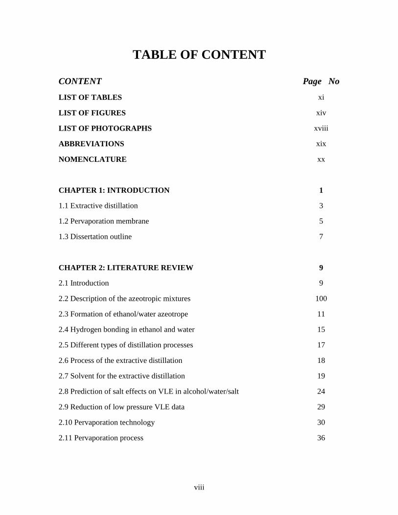
TABLE OF CONTENT
CONTENT Page No
LIST OF TABLES xi
LIST OF FIGURES xiv
LIST OF PHOTOGRAPHS xviii
ABBREVIATIONS xix
NOMENCLATURE xx
CHAPTER 1: INTRODUCTION 1
1.1 Extractive distillation 3
1.2 Pervaporation membrane 5
1.3 Dissertation outline 7
CHAPTER 2: LITERATURE REVIEW 9
2.1 Introduction 9
2.2 Description of the azeotropic mixtures 100
2.3 Formation of ethanol/water azeotrope 11
2.4 Hydrogen bonding in ethanol and water 15
2.5 Different types of distillation processes 17
2.6 Process of the extractive distillation 18
2.7 Solvent for the extractive distillation 19
2.8 Prediction of salt effects on VLE in alcohol/water/salt 24
2.9 Reduction of low pressure VLE data 29
2.10 Pervaporation technology 30
2.11 Pervaporation process 36
ix
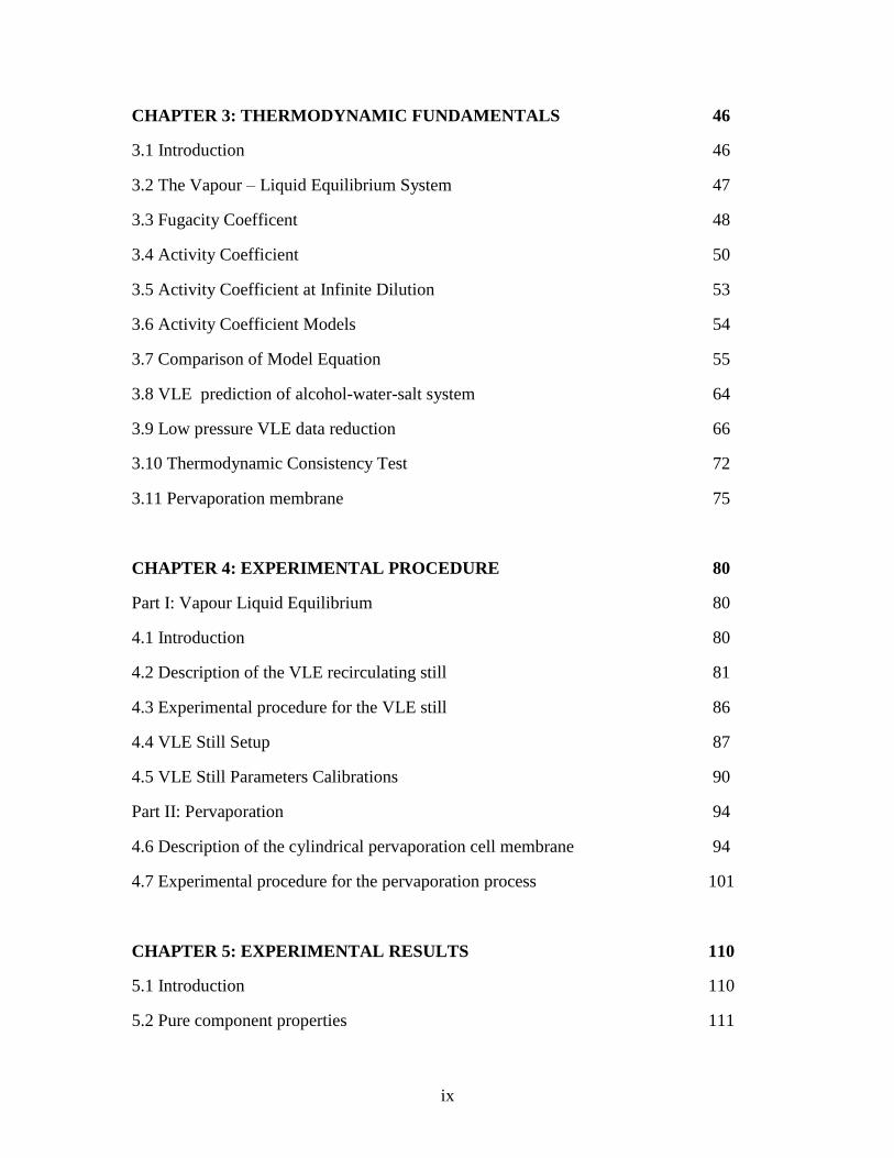
CHAPTER 3: THERMODYNAMIC FUNDAMENTALS 46
3.1 Introduction 46
3.2 The Vapour – Liquid Equilibrium System 47
3.3 Fugacity Coefficent 48
3.4 Activity Coefficient 50
3.5 Activity Coefficient at Infinite Dilution 53
3.6 Activity Coefficient Models 54
3.7 Comparison of Model Equation 55
3.8 VLE prediction of alcohol-water-salt system 64
3.9 Low pressure VLE data reduction 66
3.10 Thermodynamic Consistency Test 72
3.11 Pervaporation membrane 75
CHAPTER 4: EXPERIMENTAL PROCEDURE 80
Part I: Vapour Liquid Equilibrium 80
4.1 Introduction 80
4.2 Description of the VLE recirculating still 81
4.3 Experimental procedure for the VLE still 86
4.4 VLE Still Setup 87
4.5 VLE Still Parameters Calibrations 90
Part II: Pervaporation 94
4.6 Description of the cylindrical pervaporation cell membrane 94
4.7 Experimental procedure for the pervaporation process 101
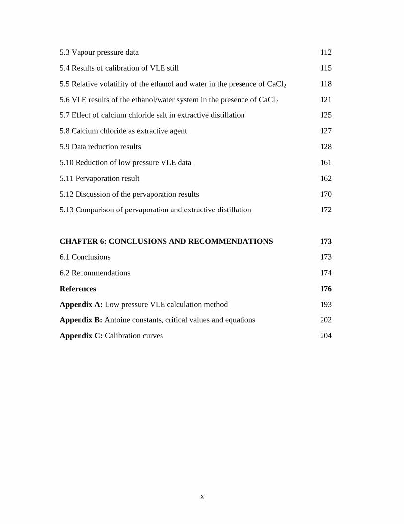
CHAPTER 5: EXPERIMENTAL RESULTS 110
5.1 Introduction 110
5.2 Pure component properties 111
x
5.3 Vapour pressure data 112
5.4 Results of calibration of VLE still 115
5.5 Relative volatility of the ethanol and water in the presence of CaCl2 118
5.6 VLE results of the ethanol/water system in the presence of CaCl2 121
5.7 Effect of calcium chloride salt in extractive distillation 125
5.8 Calcium chloride as extractive agent 127
5.9 Data reduction results 128
5.10 Reduction of low pressure VLE data 161
5.11 Pervaporation result 162
5.12 Discussion of the pervaporation results 170
5.13 Comparison of pervaporation and extractive distillation 172
CHAPTER 6: CONCLUSIONS AND RECOMMENDATIONS 173
6.1 Conclusions 173
6.2 Recommendations 174
References 176
Appendix A: Low pressure VLE calculation method 193
Appendix B: Antoine constants, critical values and equations 202
Appendix C: Calibration curves 204
xi
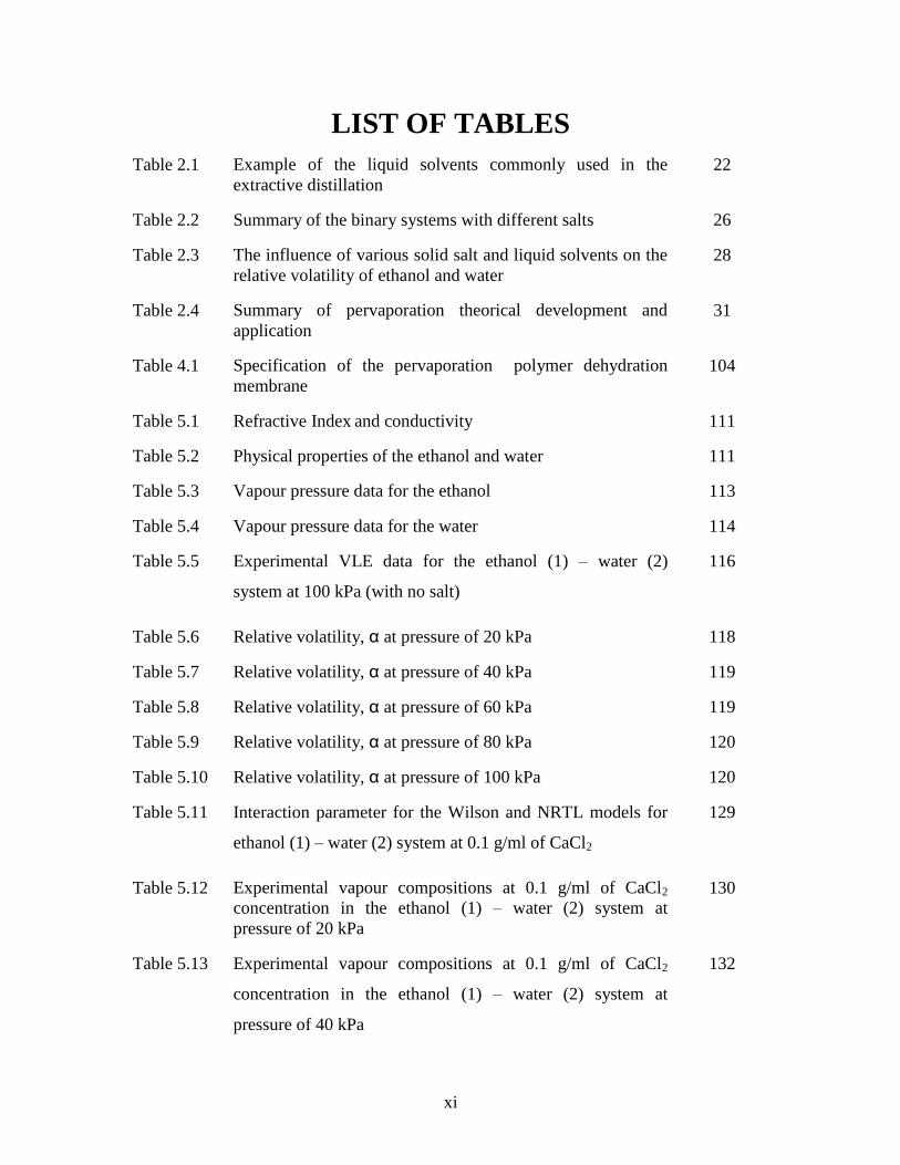
LIST OF TABLES
Table 2.1 Example of the liquid solvents commonly used in the
extractive distillation
22
Table 2.2 Summary of the binary systems with different salts 26
Table 2.3 The influence of various solid salt and liquid solvents on the
relative volatility of ethanol and water
28
Table 2.4 Summary of pervaporation theorical development and
application
31
Table 4.1 Specification of the pervaporation polymer dehydration
membrane
104
Table 5.1 Refractive Index and conductivity 111
Table 5.2 Physical properties of the ethanol and water 111
Table 5.3 Vapour pressure data for the ethanol 113
Table 5.4 Vapour pressure data for the water 114
Table 5.5 Experimental VLE data for the ethanol (1) – water (2)
system at 100 kPa (with no salt)
116
Table 5.6 Relative volatility, α at pressure of 20 kPa 118
Table 5.7 Relative volatility, α at pressure of 40 kPa 119
Table 5.8 Relative volatility, α at pressure of 60 kPa 119
Table 5.9 Relative volatility, α at pressure of 80 kPa 120
Table 5.10 Relative volatility, α at pressure of 100 kPa 120
Table 5.11 Interaction parameter for the Wilson and NRTL models for
ethanol (1) – water (2) system at 0.1 g/ml of CaCl2
129
Table 5.12 Experimental vapour compositions at 0.1 g/ml of CaCl2
concentration in the ethanol (1) – water (2) system at
pressure of 20 kPa
130
Table 5.13 Experimental vapour compositions at 0.1 g/ml of CaCl2
concentration in the ethanol (1) – water (2) system at
pressure of 40 kPa
132
xii
Table 5.14 Experimental vapour compositions at 0.1 g/ml of CaCl2
concentration in the ethanol (1) – water (2) system at
pressure of 60 kPa 136
134
Table 5.15 Experimental vapour compositions at 0.1 g/ml of CaCl2
concentration in the ethanol (1) – water (2) system at
pressure of 80 kPa
136
Table 5.16 Experimental vapour compositions at 0.1 g/ml of CaCl2
concentration in the ethanol (1) – water (2) system at
pressure of 100 kPa
138
Table 5.17 Interaction parameter for the Wilson and NRTL models for
ethanol (1) – water (2) system at 0.2 g/ml of CaCl2
140
Table 5.18 Experimental vapour compositions at 0.2 g/ml of CaCl2
concentration in the ethanol (1) – water (2) system at
pressure of 20 kPa
141
Table 5.19 Experimental vapour compositions at 0.2 g/ml of CaCl2
concentration in the ethanol (1) – water (2) system at
pressure of 40 kPa
143
Table 5.20 Experimental vapour compositions at 0.2 g/ml of CaCl2
concentration in the ethanol (1) – water (2) system at
pressure of 60 kPa
145
Table 5.21 Experimental vapour compositions at 0.2 g/ml of CaCl2
concentration in the ethanol (1) – water (2) system at
pressure of 80 kPa
147
Table 5.22 Experimental vapour compositions at 0.2 g/ml of CaCl2
concentration in the ethanol (1) – water (2) system at
pressure of 100 kPa
149
Table 5.23 Interaction parameter for the Wilson and NRTL models for
ethanol (1) – water (2) system at 0.3 g/ml of CaCl2
151
Table 5.24 Experimental vapour compositions at 0.3 g/ml of CaCl2
concentration in the ethanol (1) – water (2) system at
pressure of 20 kPa
152
xiii
Table 5.25 Experimental vapour compositions at 0.3 g/ml of CaCl2
concentration in the ethanol (1) – water (2) system at
pressure of 40 kPa
154
Table 5.26 Experimental vapour compositions at 0.3 g/ml of CaCl2
concentration in the ethanol (1) – water (2) system at
pressure of 60 kPa
156
Table 5.27 Experimental vapour compositions at 0.3 g/ml of CaCl2
concentration in the ethanol (1) – water (2) system at
pressure of 80 kPa
158
Table 5.28 Experimental vapour compositions at 0.3 g/ml of CaCl2
concentration in the ethanol (1) – water (2) system at
pressure of 100 kPa
160
Table 5.29 Refractive index at different temperatures 99% wt% ethanol 163
Table 5.30 Refractive index at different temperature for 95% wt%
ethanol
163
Table 5.31 Refractive index at different temperature for 90% wt%
ethanol
163
Table 5.32 Separation factor at feed composition of 1% water and 99%
ethanol
167
Table 5.33 Separation factor at feed composition of 5% water and 95%
ethanol
167
Table 5.34 Separation factor at feed composition of 5% water and 95%
ethanol
167
Table B1 Antoine coefficients 202
Table B2 Pure component liquid molar volumes 202
Table B3 Critical values and acentric factors for selected component 203
Table C1 GC HP 5890 series II operating parameters 205

xiv
LIST OF FIGURES
Figure 2.1 Example of an azeotropic diagram for the
ethanol/cyclohexane system at 40 kPa (a) x-y diagram and
(b) T-x-y diagram
11
Figure 2.2 Ethanol (1)-water (2) composition curve 12
Figure 2.3 VLE plot for ethanol (1)/water (2) system showing
composition curve for ethanol (1) and water (2)
13
Figure 2.4 VLE plot for the ethanol (1)/water (2) system showing liquid
composition C1 produces and vapour composition C2
14
Figure 2.5 VLE plot for the ethanol (1)/water (2) system showing liquid
composition C2 produces and vapour composition C3
15
Figure 2.6 Ethanol-water hydrogen bonding 16
Figure 2.7 Two column for extractive distillation process 18
Figure 2.8 The process of the extractive distillation with salt 21
Figure 2.9 Vacuum pervaporation process 34
Figure 2.10 Sweep gas pervaporation process 34
Figure 2.11 Schematic diagram of the pervaporation set-up 42
Figure 3.1 Block diagram for the bubble point pressure iteration for the
combined method
70
Figure 3.2 Block diagram for the bubble point temperature iteration for
the combined method
71
Figure 3.3 Pervaporation Process 76
Figure 4.1 Schematic diagram of vapour–liquid equilibrium still. 85
Figure 4.2 Schematic of the equipment layout 88
Figure 4.3 Plateau region for pure ethanol at 40 kPa 91
Figure 4.4 Cross-sectional of the cylindrical pervaporation cell 95
Figure 4.5 Top view of the cylindrical pervaporation cell 95
Figure 4.6 Cylindrical pervaporation cell 97
Figure 4.7 Schematic diagram for the pervapoartion process set-up 98
Figure 4.8 Polymer pervaporation membrane 101
xv
Figure 4.9 The pervaporation test of ethanol/water system at
temperature of 343.15 K and pressure of 80 kPa
103
Figure 5.1 Vapour pressure data of ethanol 113
Figure 5.2 Vapour pressure data of water 114
Figure 5.3 Experimental data for the ethanol (1) – water (2) system at
100 kPa with no salt
117
Figure 5.4 T-x-y diagram for the ethanol (1) – water (2) system at 100
kPa with no salt
117
Figure 5.5 Effect of CaCl2 concentration in ethanol (1) – water (2)
system at pressure of 20 kPa
121
Figure 5.6 Effect of CaCl2 concentration in ethanol (1) – water (2)
system at pressure of 40 kPa
122
Figure 5.7 Effect of CaCl2 concentration in ethanol (1) – water (2)
system at pressure of 60 kPa
122
Figure 5.8 Effect of CaCl2 concentration in ethanol (1) – water (2)
system at pressure of 80 kPa
123
Figure 5.9 Effect of CaCl2 concentration in ethanol (1) – water (2)
system at 100 kPa
123
Figure 5.10 Comparison of the CaCl2 concentration for the ethanol (1) –
water (2) system at 100 kPa 124
Figure 5.11 Comparison of the CaCl2 concentration of 0.3 g/ml for the
ethanol (1) – water (2) system at 100 kPa
124
Figure 5.12 NRTL and Wilson model fit for the ethanol (1) – water (2)
system at 0.1 g/ml CaCl2 concentration at 20 kPa
131
Figure 5.13 NRTL and Wilson model fit for the ethanol (1) – water (2)
system at 0.1 g/ml CaCl2 concentration at 40 kPa
133
Figure 5.14 NRTL and Wilson model fit for the ethanol (1) – water (2)
system at 0.1 g/ml CaCl2 concentration at 60 kPa
135
Figure 5.15 NRTL and Wilson model fit for the ethanol (1) – water (2)
system at 0.1 g/ml CaCl2 concentration at 80 kPa
137
Figure 5.16 NRTL and Wilson model fit for the ethanol (1) – water (2)
system at 0.1 g/ml CaCl2 concentration at 100 kPa
139
Figure 5.17 NRTL and Wilson model fit for the ethanol (1) – water (2) 142
xvi
system at 0.2 g/ml CaCl2 concentration at 20 kPa
Figure 5.18 NRTL and Wilson model fit for the ethanol (1) – water (2)
system at 0.2 g/ml CaCl2 concentration at 40 kPa
144
Figure 5.19 NRTL and Wilson model fit for the ethanol (1) – water (2)
system at 0.2 g/ml CaCl2 concentration at 60 kPa
146
Figure 5.20 NRTL and Wilson model fit for the ethanol (1) – water (2)
system at 0.2 g/ml CaCl2 concentration at 80 kPa
148
Figure 5.21 NRTL and Wilson model fit for the ethanol (1) – water (2)
system at 0.2 g/ml CaCl2 concentration at 100 kPa
150
Figure 5.22 NRTL and Wilson model fit for the ethanol (1) – water (2)
system at 0.3 g/ml CaCl2 concentration at 20 kPa
153
Figure 5.23 NRTL and Wilson model fit for the ethanol (1) – water (2)
system at 0.3 g/ml CaCl2 concentration at 40 kPa
155
Figure 5.24 NRTL and Wilson model fit for the ethanol (1) – water (2)
system at 0.3 g/ml CaCl2 concentration at 60 kPa
157
Figure 5.25 NRTL and Wilson model fit for the ethanol (1) – water (2)
system at 0.3 g/ml CaCl2 concentration at 80 kPa
159
Figure 5.26 NRTL and Wilson model fit for the ethanol (1) – water (2)
system at 0.3 g/ml CaCl2 concentration at 100 kPa
161
Figure 5.27 Water flux at different temperatures 164
Figure 5.28 Water flux at different pressures 164
Figure 5.29 Product purity for feed composition of 10% water and 90%
ethanol
165
Figure 5.30 Product purity for feed composition of 5% water and 95%
ethanol
165
Figure 5.31 Product purity for feed composition of 1% water and 99%
ethanol
166
Figure 5.32 Separation factor achieved for ethanol-water at feed
composition of 1%, 5% and 10% water at 313.15 K
168
Figure 5.33 Separation factor achieved for ethanol-water at feed
composition of 1%, 5% and 10% water at 323.15 K
168
Figure 5.34 Separation factor achieved for ethanol-water at feed
composition of 1%, 5% and 10% water at 333.15 K
169
xvii
Figure 5.35 Separation factor achieved for ethanol-water at feed
composition of 1%, 5% and 10% water at 343.15 K
169
Figure C1 VLE still calibration with ethanol (1) –water (2) system at
100 kPa with no salt
204
Figure C2 Temperature probe calibration for the VLE still 204
Figure C3 Pressure transducer calibration for the VLE still 205
Figure C4 GC HP 5890 series II calibration with concentrated ethanol
(1) and water (2) system
206
Figure C5 Inverse GC HP 5890 series II calibration with dilute ethanol
(1) and water (2) system
206

xviii
LIST OF PHOTOGRAPHS
Photograph 4.1 Vapour-liquid equilibrium still set-up 89
Photograph 4.2 The HP 5890 series II (TCD) gas chromatography 93
Photograph 4.3 Karl-Firscher instrument 100
xix
ABBREVIATIONS
ACN Acetonitrile
AD Azeotropic Distillation
ASOG Analytical Solution Of Group
DMF Dimethethylformanide
ED Extractive Distillation
EOS Equation Of State
FID Flame Ionization Detector
GC Gas Chromatograph
GE Excess molar Gibbs free energy
HP Hewlett Packard
LPVLE Low Pressure Vapour Liquid Equilibrium
NFM N-Formylmorpholine
NMP N-Methylpyrrolidone
NRTL Non-Random Two Liquids
TCD Thermal Conductivity Detector
THF Tetrahydrofuran
T-K Wilson Tsuboka-Katayama Wilson activity coefficient model
UNIQUAC UNIversal QUAsi-Chemical
UNIFAC Universal quasi-chemical Functionally Group of Activity Coefficient
VLE Vapour Liquid Equilibrium
xx
NOMENCLATURE
A Adjustable parameter in correlating equations, GC peak area,
cubic EOS constant
-
B Second viral coefficient -
f Fugacity -
F Difference between the number of variables -
G Gibbs energy kJ/kg
G Gibbs energy kJ/kg
H Enthalpy kJ/kg
K Distribution coefficient for component i -
l Membrane thickness m
N Number of component -
P Pressure kPa
q Parameter of the pure component molecular structure constants -
r Parameter of the pure component molecular structure constants -
R Universal gas constant kJ/kg.K
T Temperature K
v Specific volume m3/kg
V Molar volume m3
x Mole fraction of component i in liquid phase -
y Mole fraction of component i in vapour phase -
Z Compressibility -
xxi
Greek symbols
Vapour pressure correlation for cubic EOS, parameter mixing rules,
adjustable parameter in correlating equations
Constant or function in the T-K Wilson equations
Activity coefficient
Chemical potential
Fugacity coefficient
Nonideality term in the LPVLE gamma-phi method, constant or function in
the UNIQUAC equation, polarity factor in the Tarakad-Danner method
Adjustable interaction parameter in the Wilson and T-K Wilson equations
Parameter in the cubic EOS (TR, ) correlation
Constant or function in the Wilson and T-K Wilson equations
Constant or function in the UNIQUAC and UNIFAC equations
Density
Constant or function in the UNIQUAC and NRTL equations
Chemical species distributed at equilibrium
Acentric factor
UNIFAC group interaction parameter
∞ Infinite dilution
Superscripts
calc Calculated quantity
E Excess quantity
G Gas permeability
L Liquid phase
sat Saturation state pure component quantity
xxii
V Vapour phase
Subscripts
c Critical
i Component identity
j Component identity
l Liquid through the membrane
1
CHAPTER 1
INTRODUCTION
Fuel grade bioethanol production has gained attention recently because of two main
reasons. First, it is gradually/frequently being used as a fuel oxygenate in place of methyl
t-butyl ether (MTBE). The second reason relates to its potential to be used as an alternate
fuel. Bioethanol fuel is mainly produced by the sugar fermentation process; although it
can also be manufactured by the chemical process or as a byproduct of some chemical
processes (Vane, 2005a). The main sources of ethanol are sugar and crops. Crops are
grown specifically for energy use and include corn, maize and wheat crops, waste straw,
willow and popular tress, sawdust, reed canary grass, cord grasses, jerusalem artichoke,
myscanthus and sorghum plants (O‟Brien and Craig, 1996). There is also ongoing
research into the use of municipal solid waste to produce ethanol fuel.
Ethanol or ethyl alcohol (C2H5OH) is a clear colourless liquid, which is biodegradable,
low in toxicity and causes little environmental pollution if spilt (O‟Brien and Craig,
1996). Ethanol burns to produce carbon dioxide and water. It reduces pollution associated
2
with petroleum products such as SOx and NOx. Ethanol is a high octane fuel and has
replaced lead as an octane enhancer in petrol (Vane 2005a).
Bioethanol and biodiesel are the alternative fuels that can be used. The production of
alternative fuel is due to the realization that crude oil stocks are limited, hence the swing
towards more renewable sources of energy. Bioethanol and biodiesel have received
increasing attention as excellent alternative fuels and have virtually limitless potential for
growth. However, the main challenge facing bioethanol production is the separation of
high purity bioethanol, because bioethanol contains water. The separation of ethanol from
water is difficult because of the existence of an azeotrope in the mixture. The two
traditional methods of high purity ethanol separation are:
Extractive distillation
Azeotropic distillation
Other three emerging techniques are:
Salt distillation
Pressure swing distillation
Pervaporation
The purpose of this study is to explore the application of emerging technologies for the
extractive distillation and pervaporation for high purity ethanol production manipulating
the operation pressure and temperature to influence azeotropic point. In extractive
distillation, salt is added as the third component and pervaporation is the direct
separation, without salt addition.
The objective of this project was to optimize and compare the performance of
pervaporation and extraction distillation in order to produce high purity ethanol:
Study the effect of various parameters (i) operating pressure, (ii) operating
temperature, and feed composition on pervaporation.
Study the effect of salt as a separating agent and operating pressure in extractive
distillation.
3
The research was undertaken in the Department of Chemical Engineering at the Durban
University of Technology. The application of (CaCl2) salt in the extractive distillation
was investigated using the dynamic low pressure vapour-liquid equilibrium (VLE) still,
which was designed by Raal (Raal and Mühlbauer, 1998). The application of
pervaporation was investigated using a test unit built specifically for this study. In this
study, high purity ethanol was diluted with distil water and used to represent the
properties of bioethanol.
1.1 Extractive distillation
Extractive distillation is commonly applied in industry, and is becoming an important
separation method in chemical engineering. In this study, extractive distillation was
considered as a separation technique for ethanol-water system using a dissolved salt as a
separating agent. The salt used was calcium chloride which has a high boiling point.
Extractive distillation is the distillation in the presence of a component/solvent which is
not volatile when compared to the separated components. The solvent is charged
continuously near the top of the distilling column so that the concentration is maintained
on all plates of the column (Hilmen, 2000). The main characteristic of extractive
distillation is that the solvent with a high boiling point is charged to the components to be
separated so as to increase the relative volatility of one component. The experimental
vapour-liquid equilibrium (VLE) data obtained using the salt as a separating agent plays
an important role in the design of extractive distillation columns.
Separation sequence of the columns combination with other separation processes, tray
configuration and operation policy are described in full by Hilal et al., (2002). Since the
solvent plays an important role in design of extractive distillation, such conventional and
novel separating agents as solid salt, liquid solvent, the combination of liquid and solid
salt, and ionic liquids are covered in this chapter. Selection of a suitable solvent/salt is
fundamental to ensure an effective and economical design (Zhigang et al., 2005).
Ethanol forms minimum-boiling azeotropes with water at about 90 mol% ethanol.
Extractive distillation is a technique used for the separation of minimum boiling binary
4
azeotropes by the use of a solvent/salt that has the heaviest species in the mixture and
does not form any azeotropes with the original components. The solvent should be
completely miscible with the original components.
A small concentration of salt is capable of increasing the relative volatility of the more
volatile component of the solvent mixture to be distilled (Mario and Jamie, 2003). This is
known as the salt effect which is due to preferential solvation of the ions (formed when
the salt dissociates in solution) by the less volatile component of the solvent mixture
(Mario and Jamie, 2003). Ethanol is a more volatile component. Ethanol is “salted out”
from the liquid phase to the vapour phase.
Salt effects on vapour-liquid equilibria are important in extractive distillation (Lei et al.,
2002 and 2003) when the salt is used as a separating agent. However, the complex
molecule-molecule, ion-molecule and ion-ion interactions in salt-water-alcohol systems
pose a significant challenge to the development of a theoretical description of the system
(Mario and Jamie, 2003). The effect of different salts on the relative volatility of ethanol
and water was investigated (Duan et al., 1980 and Zhigang et al., 2005). It was found that
some salts produce the large salt effect on the system and the results are tabulated in
Table 2.2 Zhigang et al. (2005) arranged the order of salt effect: AlCl3 > CaCl2 > NaCl2,
Al(NO3)3 > Cu(NO3)2 > KNO3. In this study, the choice of calcium chloride was reported
by previous work such as that cited above, which indicates that calcium chloride provides
the largest salting out effect on ethanol. In addition, it is also a cheap and common salt. In
this study, calcium chloride is the salt chosen for further investigation because it has the
large salting out effect, it is a common salt and it is cheap.
It was found that calcium chloride could completely eliminate the azeotrope at the high
concentrations and increase the relative volatility. The system of ethanol/water/calcium
chloride was generally regressed using Gibbs excess energy models in particular Wilson
and NRTL. The benefits of the Wilson and NRTL parameters and consistent VLE data
are indispensable to the process industry. In light of the current environmental regulations
and given that energy efficiency and optimisation are the focus of the process industry,
experimental VLE data and ongoing research in the analysis of the data are critical to
both the improvement of current processes and the efficient design of future processes.
5
1.2 Pervaporation membrane
Pervaporation is a membrane separation process for liquid mixtures in which the initial
solution comes in contact with the internal surface of a membrane module, permeate in
the form of vapours with a low partial pressure was removed from its outer surface
(Belyaev et al., 2003). Pervaporation membrane separation can be considered as one
effective method and energy-saving process for the separation of the ethanol/water
azeotropic system (Huang et al., 2008; Huang, 1991; Shao and Huang, 2006 and Wang et
al., 2007). Pervaporation through hydrophobic membranes is potentially economically
competitive with distillation, especially for small to medium scale application (Vane,
2005a). In general, separation by pervaporation can be perfomed using membranes based
on the solution-diffusion mechanism of transport. The mass transport through the
permselective membranes involves three steps: (i) sorption of the penetrant from the feed
to the membrane, (ii) diffusion of the penetrant in the membrane, and (iii) desorption of
the penetrant from the membranes on the downstream side of the membrane (Xu et al.,
2006). The pervaporation membrane has the added advantage in that it facilitates the
direct separation of the azeotrope without the addition of the third component. Hence it
reduces the capital and operating cost that may be associated with solvent recovery.
Pervaporation theory has advanced greatly since its introduction in the early 1950‟s,
however it was only in recent years that research in this field have intensified. There has
been a noticeable increase in the number of publications concerning membrane
separation yet the technology is still far from perfect (Yampolskii and Volkov, 1991;
Neel, 1991; Binning et al., 1961 and Mulder et al., 1985) are all prominent names in
pervaporation and have written many papers of great significance. Pervaporation‟s
potential versatility ensures its place in separation technology. It is only due to a lack of
familiarity and poor knowledge of the weakness of pervaporation that inhibits its growth
industrially. This should not be a problem in the future as new and improved membranes
are constantly being produced, offering better selectivity and better resistance
(chemically and thermally). Most of the liquid mixtures could be separated using
pervaporation, yet research has concentrated on the separation of azeotropic and close
6
boiling mixtures due to difficulty in separating these mixture via conventional means
(Driolli et al., 1993).
By definition, the separation factor is equal to the ratio of the concentration of the
permeant in the permeate to the concentration of the permeant in the feed, where the
permeant is the component that is preferentially transported through the membrane. The
separation of the ethanol/water system obtained by the researchers on the pervaporation is
comparable to that obtainable in distillation systems though the transport rate of one
kg.m-2
.h-1
is far too low for industrial throughputs.
In this study, the recovery of pure ethanol from a feed stream of 90 – 99% wt% ethanol
was studied. The pervaporation operating pressure and operating temperature were varied
from 20 kPa to 80 kPa and 313.15 K to 343.15 K respectively.
7
1.3 Dissertation outline
Chapter 1
The introduction outlines the purpose of this study. It provides the background
information on the utility of the extraction distillation using calcium chloride salt as a
separating agent and the pervaporation process in order to recover high purity ethanol.
Chapter 2
This chapter reviews literature which deals with the application of emerging technologies
of extractive distillation and pervaporation process for high purity ethanol production.
Some concepts to understand and formation of destruction of azoetropes are also
presented.
Chapter 3
Chapter 3 represents information about the thermodynamic fundamentals of the
extractive distillation and pervaporation process. Data reduction schemes to predict the
effect of salt on the behavior of the ethanol-water system are also presented.
Chapter 4
This chapter is devoted to the experimental and analysis procedures and methods used for
the evaluation of salts as an extractive agent and the pervaporation studies. The analytical
techniques used for both these studies are also presented in this chapter.
Chapter 5
This chapter contains the results and discussion obtained from:
The study of the effect of salt in the separation of ethanol-water mixture.
The pervaporation studies of ethanol and water mixture.
The data reduction methods used in the vapour-liquid equilibrium studies.
8
Chapter 6
In chapter 6, conclusions and recommendations related to the effect of salt in the
extractive distillation process, and direct separation of ethanol-water system using
pervaporation to achieve high purity ethanol production are made.
9
CHAPTER 2
LITERATURE REVIEW
2.1 Introduction
To understand the separation difficulties associated with the ethanol-water system, it is
necessary to outline the phenomenon that contributes to non-ideal VLE behavior, and
how the non-ideal VLE behavior may be overcome. In this chapter a review is presented
on:
Azeotropy and its formation in the ethanol-water system.
Brief overviews of methods to employ overcome the azeotropic behavior.
Review of the use of salt as an extraction agent in extractive distillation and the
use of pervaporation technology for high purity ethanol separation.
10
2.2 Description of azeotropic mixtures
The term azeotrope means “nonboiling by any means/way” (Greek: a – non, zeo – boil,
tropos – means/way), and denotes a mixture of two components that at equilibrium, the
vapour and liquid composition are equal at a given pressure and temperature. Azeotropic
mixtures require special methods to facilitate their separation. There was a need to search
for a separating agent other than different method that consumes a lot of energy. The
separating agent might be a membrane material for pervaporation and either solvent or
addition of salt in the extractive distillation. An introduction to the phenomena of
azeotropy and non-ideal vapour-liquid equilibrium behavior will be given before
considering the various methods to separate azeotropic mixtures. Separation of
homogenous liquid mixtures (bioethanol and water) requires the creation or addition of
another phase within the system (Smith, 1995). Separation of a liquid mixture by
distillation is dependent on the partial vaporization of the liquid into a liquid and vapour
samples in which their composition may differ. The vapour phase becomes enriched in
the more volatile component. It was depleted in the less volatile components with respect
to its equilibrium, liquid phase. An azeotrope could not be separated by ordinary
distillation since no further enrichment of the vapour phase occurs. In most cases,
azeotropic mixtures require special methods to facilitate their separation such method
utilizes a mass separating agent other than energy that causes or enhances a selective
mass transfer of the azeotropic forming component.
11
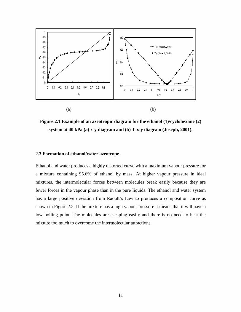
(a) (b)
Figure 2.1 Example of an azeotropic diagram for the ethanol (1)/cyclohexane (2)
system at 40 kPa (a) x-y diagram and (b) T-x-y diagram (Joseph, 2001).
2.3 Formation of ethanol/water azeotrope
Ethanol and water produces a highly distorted curve with a maximum vapour pressure for
a mixture containing 95.6% of ethanol by mass. At higher vapour pressure in ideal
mixtures, the intermolecular forces between molecules break easily because they are
fewer forces in the vapour phase than in the pure liquids. The ethanol and water system
has a large positive deviation from Raoult‟s Law to produces a composition curve as
shown in Figure 2.2. If the mixture has a high vapour pressure it means that it will have a
low boiling point. The molecules are escaping easily and there is no need to heat the
mixture too much to overcome the intermolecular attractions.
12
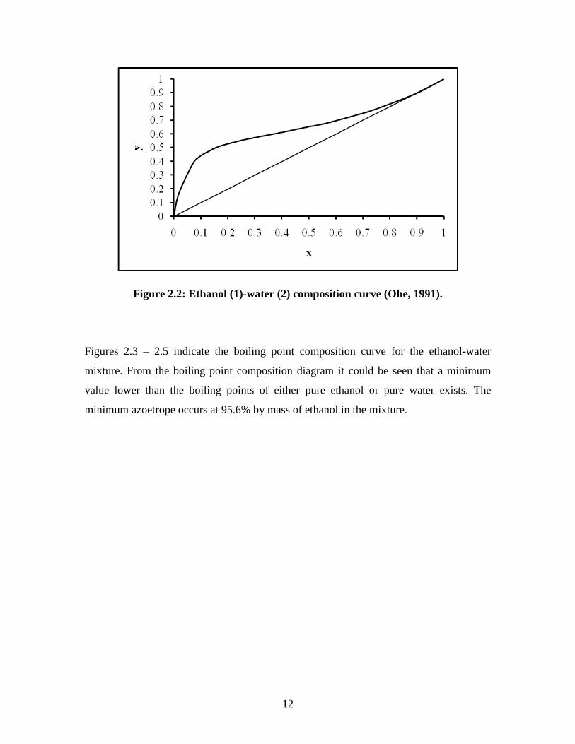
Figure 2.2: Ethanol (1)-water (2) composition curve (Ohe, 1991).
Figures 2.3 – 2.5 indicate the boiling point composition curve for the ethanol-water
mixture. From the boiling point composition diagram it could be seen that a minimum
value lower than the boiling points of either pure ethanol or pure water exists. The
minimum azoetrope occurs at 95.6% by mass of ethanol in the mixture.

13
Figure 2.3: VLE plot for ethanol (1)/water (2) system showing composition curve for
ethanol (1) and water (2) (Ohe, 1991).
By distilling a mixture of ethanol and water with composition C1 as shown in Figure 2.4,
it boils at certain temperature by the liquid curve and produces vapour with composition
C2.
14
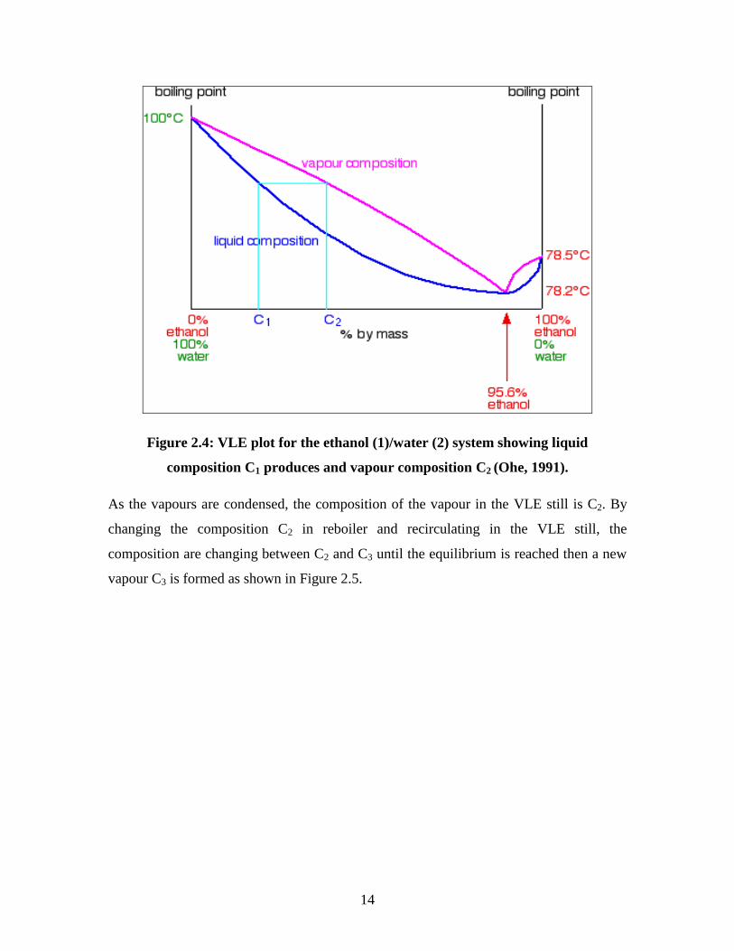
Figure 2.4: VLE plot for the ethanol (1)/water (2) system showing liquid
composition C1 produces and vapour composition C2 (Ohe, 1991).
As the vapours are condensed, the composition of the vapour in the VLE still is C2. By
changing the composition C2 in reboiler and recirculating in the VLE still, the
composition are changing between C2 and C3 until the equilibrium is reached then a new
vapour C3 is formed as shown in Figure 2.5.
15
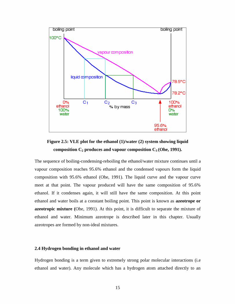
Figure 2.5: VLE plot for the ethanol (1)/water (2) system showing liquid
composition C2 produces and vapour composition C3 (Ohe, 1991).
The sequence of boiling-condensing-reboiling the ethanol/water mixture continues until a
vapour composition reaches 95.6% ethanol and the condensed vapours form the liquid
composition with 95.6% ethanol (Ohe, 1991). The liquid curve and the vapour curve
meet at that point. The vapour produced will have the same composition of 95.6%
ethanol. If it condenses again, it will still have the same composition. At this point
ethanol and water boils at a constant boiling point. This point is known as azeotrope or
azeotropic mixture (Ohe, 1991). At this point, it is difficult to separate the mixture of
ethanol and water. Minimum azeotrope is described later in this chapter. Usually
azeotropes are formed by non-ideal mixtures.
2.4 Hydrogen bonding in ethanol and water
Hydrogen bonding is a term given to extremely strong polar molecular interactions (i.e
ethanol and water). Any molecule which has a hydrogen atom attached directly to an
16
oxygen or nitrogen is capable of hydrogen bonding. These molecules have higher boiling
points when compared to similar size of molecules which not have an –O-H or an –N-H
group. The hydrogen bonding makes the molecules “stickier” and more heat is necessary
to separate them (Ophardt, 2003). Solutions that exhibit hydrogen bonding generally
exhibit azeotropic behavior. In this study of the ethanol/water mixture, ethanol has a
hydrogen atom attached directly to oxygen and this oxygen still has exactly the same two
lone pairs as in a water molecule. Hydrogen bonding can occur between ethanol
molecules although not as effectively as in water (Ophardt, 2003). Mixing involves
breaking hydrogen bonds between water molecules. Breaking hydrogen bonds between
ethanol molecules makes a strong stickier hydrogen bond between water and ethanol
molecules. This increases with increasing ethanol concentration hence the mixture
becomes difficult to separate beyond a certain concentration (i.e at 90 mol% ethanol and
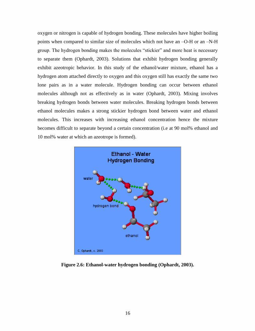
10 mol% water at which an azeotrope is formed).
Figure 2.6: Ethanol-water hydrogen bonding (Ophardt, 2003).
17
2.5 Different types of distillation processes
The separation of azeotropic systems can be achieved by the addition of a suitable
solvent, which influences the activity coefficient and relative volatility. Six methods for
separating azeotropic mixtures as described by Stichimar et al. (1989) follow:
Extractive distillation – a high boiling solvent is added near the top of the column to
favourably alter the relative volatility in order to separate the components. A second
column separates the bottom in order to recycle the solvent.
Homogeneous azeotropic distillation – the liquid separating agent is completely
miscible.
Heterogeneous azeotropic distillation, more commonly, Azeotropic Distillation –
where the liquid separating agent, called the entrainer or solvent, forms one or more
azeotropes with the other components in the mixture and causes two liquid phases to
exit over a wide range of compositions. This immiscibility is the key to making the
distillation sequence work.
Distillation using salts – the salts dissociates in the liquid mixture and alters the
relative volatilities sufficiently that the separation becomes possible.
Pressure swing distillation – a series of columns operating at different pressures are
used to separate binary azeotropes which change appreciably in composition over a
moderate pressure range or where a separating agent which forms a pressure-sensitive
azeotrope is added to separate a pressure-insensitive azeotrope.
Reactive distillation – the separating agent reacts preferentially and reversibly with
one of the azeotropic constituents. The reaction product is then distilled from the non-
reacting components and the reaction is reversed to recover the initial component.
Since the project focuses on two separation techniques namely extractive distillation with
salt and pervaporation, both technologies are reviewed.
18
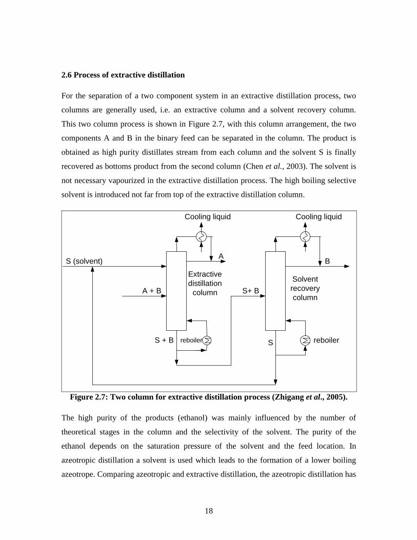
2.6 Process of extractive distillation
For the separation of a two component system in an extractive distillation process, two
columns are generally used, i.e. an extractive column and a solvent recovery column.
This two column process is shown in Figure 2.7, with this column arrangement, the two
components A and B in the binary feed can be separated in the column. The product is
obtained as high purity distillates stream from each column and the solvent S is finally
recovered as bottoms product from the second column (Chen et al., 2003). The solvent is
not necessary vapourized in the extractive distillation process. The high boiling selective
solvent is introduced not far from top of the extractive distillation column.
S (solvent)
A + B
A
S+ B
S + B S
B
Cooling liquid Cooling liquid
reboilerreboiler
Solvent
recovery
column
Extractive
distillation
column
Figure 2.7: Two column for extractive distillation process (Zhigang et al., 2005).
The high purity of the products (ethanol) was mainly influenced by the number of
theoretical stages in the column and the selectivity of the solvent. The purity of the
ethanol depends on the saturation pressure of the solvent and the feed location. In
azeotropic distillation a solvent is used which leads to the formation of a lower boiling
azeotrope. Comparing azeotropic and extractive distillation, the azeotropic distillation has
19
the disadvantage that in contrast to solvents used for extractive distillation, the solvent
has to be vaporized, which results in the higher energy consumption.
Liquid/solid as a separation agent in extractive distillation
In general organic compounds are used as selective solvents. For a safe and efficient
operation, all selective solvents for separation process should have the following desired
properties (Zhigang et al., 2005):
High selectivity
High capacity
No separation problems in the required regeneration step
High thermal and chemical stability
Low melting point
Non-toxic
Low viscosity
Negligible corrosivity
Low price
Simple purification
A high selectivity means a pure product and a higher distribution coefficient requires a
lower solvent to feed ratio. In order to have little or no impurities in the distillate of the
extractive distillation column and also to avoid separation problems in the regeneration
column, the selective solvent for extractive distillation should have a higher boiling point
than the components. High boiling point of solvent or separating agent means that at the
top distillation column, only one component is more volatile.
2.7 Solvent for extractive distillation
Separation process and solvent selection (separation agent) are factors that influence the
extractive distillation process. When a basic solvent is found, this solvent should be
further optimized to improve the separation ability and decrease the solvent ratio and
20
liquid load of the extractive distillation column (Zhigang et al., 2005). The solvent is the
core of extractive distillation. It is well known that selection of the most suitable solvent
plays an important role in the economical design of extractive distillation. To date there
are four kinds of solvents used in extractive distillation, i.e. solid salt, liquid solvent, the
combination of liquid and solid salt, and ionic liquid (Zhigang et al., 2005).
Extractive distillation with solid salt
In the systems were solubility permits, it is feasible to use a solid salt dissolved in the
liquid phase, rather than a liquid additive, as the separating agent for extractive
distillation (Zhigang et al., 2005). The extractive distillation process in which the solid
salt is used as the separating agent is called extractive distillation with solid salt. Ionic
liquids are not included as solid salts although they are a kind of salt (Zhigang et al.,
2005). Ionic liquids are described later in this chapter. Salt effect in the vapour liquid
equilibrium (VLE) refer to the ability of a solid salt which has been dissolved in a liquid
phase consisting of two or more volatile components to alter the composition of the
equilibrium vapour without salt being present in the vapour. The feed component in
which the equilibrium vapour is enhanced, is referred as “salting-out” by the salt,
otherwise, if the equilibrium vapour is not reached then the component is known as
“salting-in”.
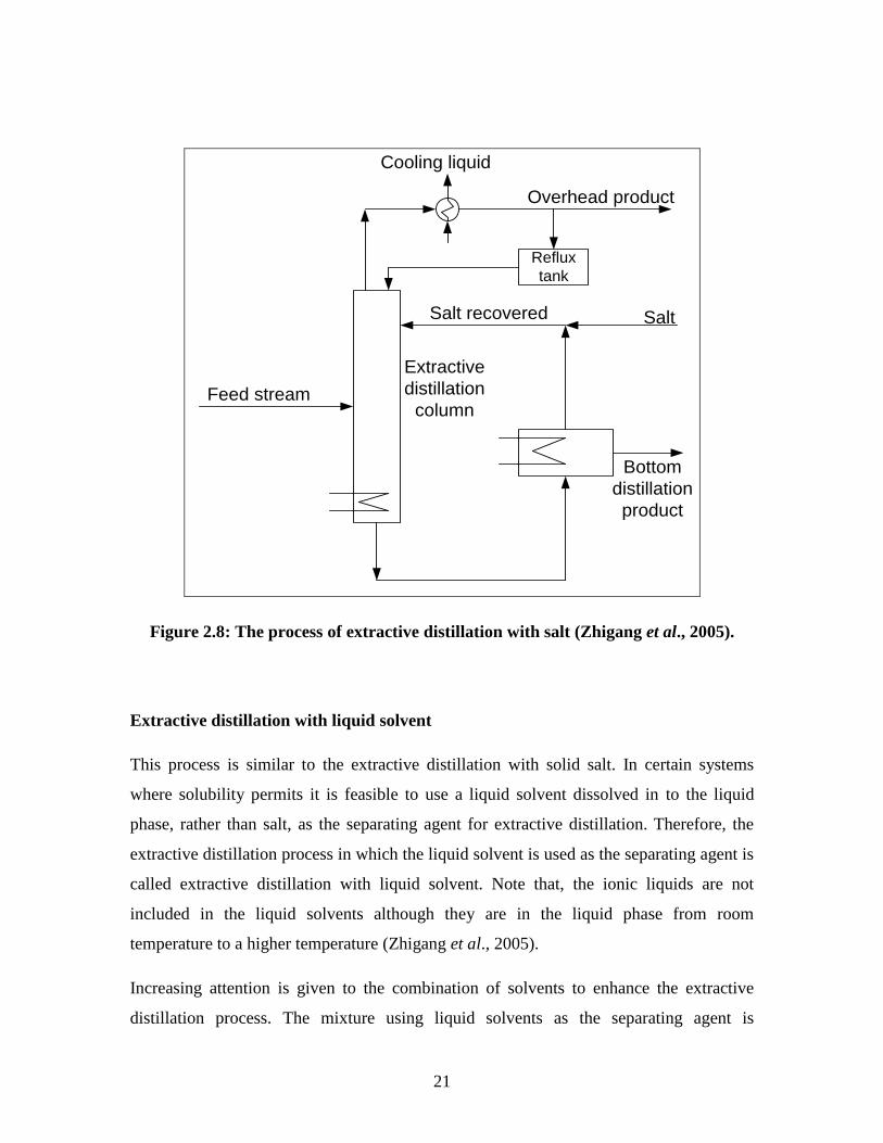
The process of extractive distillation with salt is different from the process shown in
Figure 2.7, in that the salt is not recovered by means of distillation. The extractive
distillation process can be taken as consisting of one extractive distillation column and
one solvent recovery equipment. Figure 2.8 demonstrates a typical flow sheet for salt-
effect extractive distillation. The solid salt which must be soluble to some extent in both
feed components is fed at the top of the column by dissolving it at a steady state into the
boiling reflux just prior to entering the column (Zhigang et al., 2005). The solid salt being
non-volatile flows downwards in the column. One advantage of the process of extractive
distillation with salt is that the salt is not difficult to recover, it is recovered by
evaporation.
21
Overhead product
Feed stream
Salt recovered
Reflux
tank
Cooling liquid
Extractive
distillation
column
Salt
Bottom
distillation
product
Figure 2.8: The process of extractive distillation with salt (Zhigang et al., 2005).
Extractive distillation with liquid solvent
This process is similar to the extractive distillation with solid salt. In certain systems
where solubility permits it is feasible to use a liquid solvent dissolved in to the liquid
phase, rather than salt, as the separating agent for extractive distillation. Therefore, the
extractive distillation process in which the liquid solvent is used as the separating agent is
called extractive distillation with liquid solvent. Note that, the ionic liquids are not
included in the liquid solvents although they are in the liquid phase from room
temperature to a higher temperature (Zhigang et al., 2005).
Increasing attention is given to the combination of solvents to enhance the extractive
distillation process. The mixture using liquid solvents as the separating agent is
22
complicated and interesting. According to the aims of adding one solvent to another, it
can be divided into two categories: increasing separation ability and decreasing the
boiling point of the mixture (Zhigang et al., 2005).The most important factor in selecting
the solvents is to improve the relative volatility. As a result, when one basic solvent is
given, the key objective of adding a co-solvent to the mixture is to improve the relative
volatility and to decreases the solvent ratio and liquid load of the extractive distillation
column (Zhigang et al., 2005).
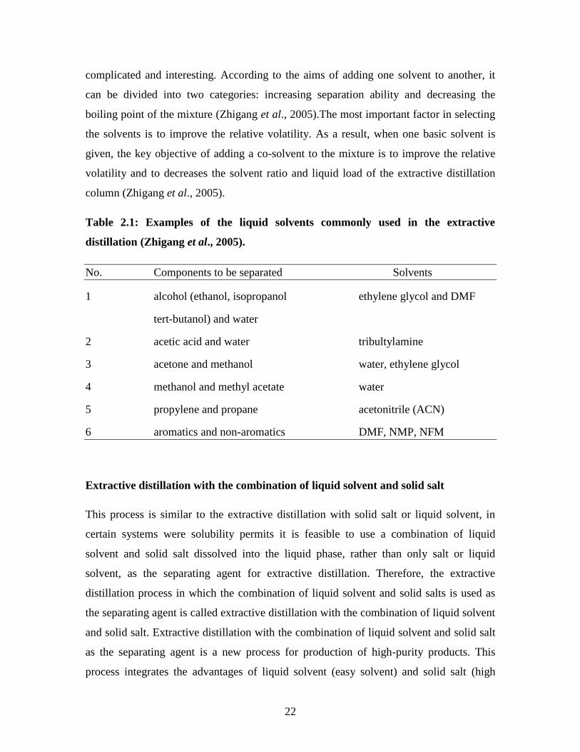
Table 2.1: Examples of the liquid solvents commonly used in the extractive
distillation (Zhigang et al., 2005).
No. Components to be separated Solvents
1 alcohol (ethanol, isopropanol ethylene glycol and DMF
tert-butanol) and water
2 acetic acid and water tribultylamine
3 acetone and methanol water, ethylene glycol
4 methanol and methyl acetate water
5 propylene and propane acetonitrile (ACN)
6 aromatics and non-aromatics DMF, NMP, NFM
Extractive distillation with the combination of liquid solvent and solid salt
This process is similar to the extractive distillation with solid salt or liquid solvent, in
certain systems were solubility permits it is feasible to use a combination of liquid
solvent and solid salt dissolved into the liquid phase, rather than only salt or liquid
solvent, as the separating agent for extractive distillation. Therefore, the extractive
distillation process in which the combination of liquid solvent and solid salts is used as
the separating agent is called extractive distillation with the combination of liquid solvent
and solid salt. Extractive distillation with the combination of liquid solvent and solid salt
as the separating agent is a new process for production of high-purity products. This
process integrates the advantages of liquid solvent (easy solvent) and solid salt (high
23
separation ability). The extractive distillation with the combination of liquid solvent and
solid salt can be suitable either for the separation of polar systems or for the separation of
non-polar systems respectively (Zhigang et al., 2005).
Extractive distillation with ionic liquid
This process is similar to the extractive distillation with solid salt or liquid solvent or the
combination, in certain systems where solubility permits it is feasible to use an ionic
liquid dissolved into the liquid phase, rather than only salt or liquid solvents, as the
separating agent for extractive distillation. Therefore, the extractive distillation process
where ionic liquid is used as the separating agent is called extractive distillation with
ionic liquid. Ionic liquids are salts consisting entirely of ions. Ionic liquid are called
“green” solvents. Most ionic liquids exhibit high thermal and chemical stability when
compared to some of the commonly used high rated solvents such as acetonitrile (ACN),
dimethethylformanide (DMF) and N-methyl-pyrrolidone (NMP), these solvents can
decompose under their separation operating conditions (Zhigang et al., 2005).
Extractive distillation with ionic liquids can be suitable either for the separation of polar
systems or for the separation of non-polar systems. According to Zhigang et al., (2005),
the following polar and non-polar systems ethanol/water, acetone/methanol, water/ acetic
acid, tetrahydrofuran (THF)/water and cyclohexane/benzene have been measured by
Seiler et al. (2001). It was found that the separation effect was very apparent for these
systems when certain ionic liquids were used. The challenge was to identify a suitable
ionic liquid which displayed good solubility for the specific components of interest to be
separated.
Some investigations on the use of ionic liquids as a solvent to separate ethanol-water
have been done. Calvar et al. (2007) have conducted the study on isobaric vapour liquid
equilibria for the ternary system of the ethanol + water + 1-hexyl-3-methylimidazolium
chloride ([C6mim][Cl]) and the binary systems containing the ionic liquid. These binary
systems were ethanol + [C6mim][Cl] and water + [C6mim][Cl] carried out at 101.3 kPa.
The VLE experimental data of binary and ternary systems were correlated using the
NTRL equation. It was found that by adding different concentrations of ionic liquid from
24
10% (wt) to 50% (wt), [C6mim][Cl] showed the negative effect in the system and it was
difficult to eliminate the azeotrope of the ethanol/water mixture. In previous work of
Calvar et al. (2006), the VLE of the ternary system of ethanol + water + 1-butyl-3-
methylimidazolium chloride [C4mim][Cl] was measured at 101.3 kPa. The study of
[C4mim][Cl] showed a positive effect and it was capable of eliminating the azeotrope of
the ethanol/water mixture with the concentration of ionic solvent between 10% (wt%)
and 50% (wt%).
2.8 Prediction of salt effects on VLE in alcohol/water/salt
Salt effect on the vapour-liquid equilibria is very important in extractive distillation
(Furter, 1976) when the salt was used as a separating agent. However, the complex
molecule-molecule, ion-molecule and ion-ion interactions in salt-water-alcohol systems
pose a significant challenge to the development of the theoretical stages of extractive
distillation. Many semi-empirical methods have been proposed to calculate VLE behavior
in such system (Ohe, 1998). Most of these methods describe ternary VLE by
extrapolation of constituent binary system data using binary interaction parameters.
Binary salt-water and salt-alcohol systems are then described using methods such as
those proposed by Pitzer (1973) and Chen et al. (2003) or using methods based on the
mean spherical approximation (MSA). Binary alcohol-water systems are described using
local composition models such as Wilson (1964); NRTL (Renon and Prausnitz, 1968)
and UNIQUAC (Abrams and Prausnitz, 1975) models or by use of Equations of State.
A method for the prediction of the salting effecting effect on the vapour liquid equilibria
of ternary alcohol-water-salt systems is proposed by Chou and Tanioka (1999). In this
method, the nonidealities of the liquid phase were consider by employing Tan‟s modified
Wilson model to describe the solvent-solvent interaction which can be obtained from the
original Wilson model, and the solvent-salt interaction which could be obtained by the
contribution of ion-ion and solvent-ion interaction. The estimation of the salt effect on the
vapour-liquid equilibrium data of alcohol solutions plays an important role in the
distillation process. The following models: Wilson, NRTL and UNIQUAC were verified
and are successful in predicting VLE of non-electrolyte solution.
25
Tan (1987) modified the Wilson model to predict the salting effect on the VLE of alcohol
aqueous solutions. More details will be presented in section 3.8. Tan (1987) measured
two binary solvent-solvent interaction parameters and two binary solvent-salt interaction
parameters; the solvent-solvent parameters were the same as those of the original Wilson
model, and the solvent-salt parameter could be calculated from the vapour pressure data
of the solvent-salt systems.
Kumar (1993) provides a review of theoretical and predictive models and correlation for
estimating the salt effect. The models were classified into two categories depending
whether the model is based on excess free energy or not. It was found that the models
based on excess free energy were more realistic because of the pertinent interactions in
the solution.
26
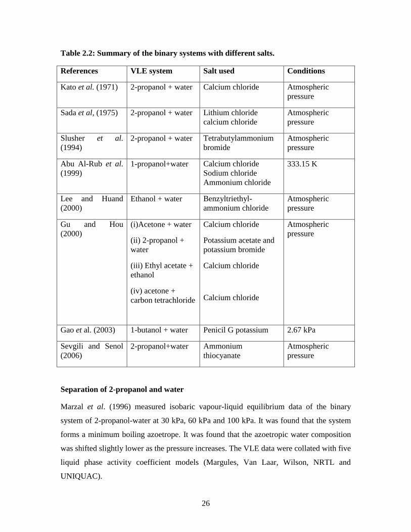
Table 2.2: Summary of the binary systems with different salts.
References VLE system Salt used Conditions
Kato et al. (1971) 2-propanol + water Calcium chloride Atmospheric
pressure
Sada et al, (1975) 2-propanol + water Lithium chloride
calcium chloride
Atmospheric
pressure
Slusher et al.
(1994)
2-propanol + water Tetrabutylammonium
bromide
Atmospheric
pressure
Abu Al-Rub et al.
(1999)
1-propanol+water Calcium chloride
Sodium chloride
Ammonium chloride
333.15 K
Lee and Huand
(2000)
Ethanol + water Benzyltriethyl-
ammonium chloride
Atmospheric
pressure
Gu and Hou
(2000)
(i)Acetone + water
(ii) 2-propanol +
water
(iii) Ethyl acetate +
ethanol
(iv) acetone +
carbon tetrachloride
Calcium chloride
Potassium acetate and
potassium bromide
Calcium chloride
Calcium chloride
Atmospheric
pressure
Gao et al. (2003) 1-butanol + water Penicil G potassium 2.67 kPa
Sevgili and Senol
(2006)
2-propanol+water Ammonium
thiocyanate
Atmospheric
pressure
Separation of 2-propanol and water
Marzal et al. (1996) measured isobaric vapour-liquid equilibrium data of the binary
system of 2-propanol-water at 30 kPa, 60 kPa and 100 kPa. It was found that the system
forms a minimum boiling azoetrope. It was found that the azoetropic water composition
was shifted slightly lower as the pressure increases. The VLE data were collated with five
liquid phase activity coefficient models (Margules, Van Laar, Wilson, NRTL and
UNIQUAC).
27
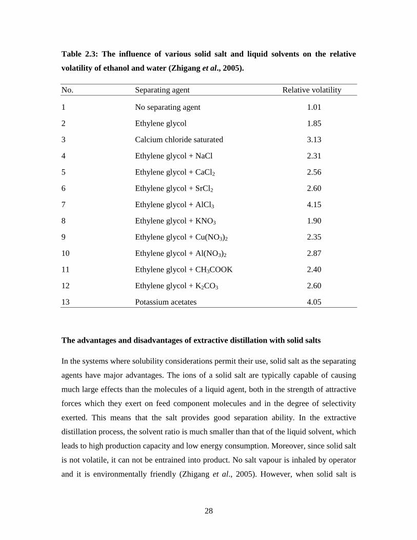
Separation of ethanol and water
Ethanol is a basic chemical material and solvent used in the production of many
chemicals and intermediates. Especially in the recent year, ethanol is paid more attention
because it is an excellent alternative fuel and has a virtually limitless potential for growth.
However, ethanol is usually diluted and required to be separated from water. It is known
that ethanol forms azeotrope with water and can not be extracted to a high concentration
from the aqueous solutions by ordinary distillation methods (Lei et al., 2002). Extractive
distillation using a 70/30 mixture of potassium and sodium acetate as the separating agent
produces < 99.8% ethanol completely free of separating agent directly from the top of the
column (Furter, 1992 and 1993). The separation of ethanol and water is the most
important application of extractive distillation with solid salt. The influence of various
salts on the relative volatility of ethanol and water was investigated (Duan et al., 1980)
and Zhigang et al., 2005) and the results are tabulated in Table 2.3 where the volume
ratio of the azetropic ethanol-water solution and the separating is 1.0 and the
concentration of salt is 0.2 g/ml. Zhigang et al., (2005) arranged the order of salt effect:
AlCl3 > CaCl2 > NaCl2, Al(NO3)3 > Cu(NO3)2 > KNO3. It was concluded that the results
in Table 2.3 revealed that the higher the valence of metal ion, the more salt effect.
28
Table 2.3: The influence of various solid salt and liquid solvents on the relative
volatility of ethanol and water (Zhigang et al., 2005).
No. Separating agent Relative volatility
1 No separating agent 1.01
2 Ethylene glycol 1.85
3 Calcium chloride saturated 3.13
4 Ethylene glycol + NaCl 2.31
5 Ethylene glycol + CaCl2 2.56
6 Ethylene glycol + SrCl2 2.60
7 Ethylene glycol + AlCl3 4.15
8 Ethylene glycol + KNO3 1.90
9 Ethylene glycol + Cu(NO3)2 2.35
10 Ethylene glycol + Al(NO3)2 2.87
11 Ethylene glycol + CH3COOK 2.40
12 Ethylene glycol + K2CO3 2.60
13 Potassium acetates 4.05
The advantages and disadvantages of extractive distillation with solid salts
In the systems where solubility considerations permit their use, solid salt as the separating
agents have major advantages. The ions of a solid salt are typically capable of causing
much large effects than the molecules of a liquid agent, both in the strength of attractive
forces which they exert on feed component molecules and in the degree of selectivity
exerted. This means that the salt provides good separation ability. In the extractive
distillation process, the solvent ratio is much smaller than that of the liquid solvent, which
leads to high production capacity and low energy consumption. Moreover, since solid salt
is not volatile, it can not be entrained into product. No salt vapour is inhaled by operator
and it is environmentally friendly (Zhigang et al., 2005). However, when solid salt is
29
used in industrial operation, dissolution reuse and transport of salt is a problem. The
concurrent blockage and erosion limit the industrial value of extractive distillation with
solid salt. That is why extractive distillation with solid salt is not widely used in industry.
2.9 Reduction of low pressure VLE data
It is very important to test experimental equilibrium data for thermodynamic consistency.
According to Prausnitz et al. (1999) the Gibbs-Duhem equation could be used to
interrelate activity coefficient of all components in a mixture. The experimental data
should obey the Gibbs-Duhem equation, if they do not, the data cannot be correct. If they
do obey the Gibbs-Duhem equation, the data is probably correct and can be used for
designing distillation column (Prausnitz et al., 1999). There are simple models for VLE
data reduction developed from excess Gibbs free energy. The choice of a correlating
equation for the excess Gibbs free energy is an important decision in data reduction, and
systems with complex behavior may require the testing of several equations before a
suitable experimental fit is found (Raal and Mühlbauer, 1998). The search for an
appropriate equation is complicated if there is much scatter in the data or if the data set is
thermodynamically inconsistent. In that case it may be necessary to re-measure the data
or to compute variables (for example, vapour composition) for which the accuracy is
suspect.
All the calculations are based on modified Raoult‟s law described in Chapter 3. In this
study, the gamma/phi method of VLE is used and includes the activity coefficient to
account for liquid-phase nonidealities, but is limited by the assumption of vapour-phase
ideality (Smith et al., 2001). Gamma/phi method of VLE, reduces to Raoult‟s law when
Фi = γi = 1, and to modified Raoult‟s law when Фi = 1.
Dewpoint and Bubblepoint calculations
When a liquid at constant pressure is heated, at the certain temperature, the first bubble of
vapour will form. This temperature in the bubble-point and it will have associated with it
an equilibrium vapour composition, yi. When the total pressure above a liquid
composition xi at constant temperature is reduced, a vapour bubble will form at a pressure
equal to the bubble-point pressure. The dew-point is the temperature at which the first
30
droplet of liquid will condense when a vapour of composition yi is cooled at constant
pressure, or when the pressure is increased at constant temperature. In addition, dew-
point and bubble point calculations may be required for process equipment design.
Bubble-point and dew-point calculations find greatest application in multi-component
distillation, since for a known or specified liquid composition it is usually necessary to
find the vapour composition and equilibrium temperature on each plate of the distillation
column (Raal and Mühlbauer, 1998). The nature of dew-point and bubble-point
calculation is evident of correct experimental data by applying Raoult‟s law and modified
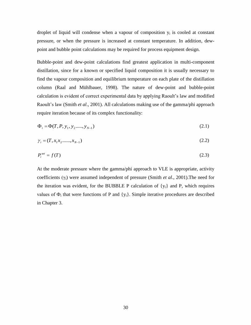
Raoult‟s law (Smith et al., 2001). All calculations making use of the gamma/phi approach
require iteration because of its complex functionality:
).....,,,,( 121 Ni yyyPT (2.1)
)......,,( 121 Ni xxxT (2.2)
)(TfP sat
i (2.3)
At the moderate pressure where the gamma/phi approach to VLE is appropriate, activity
coefficients (γi) were assumed independent of pressure (Smith et al., 2001).The need for
the iteration was evident, for the BUBBLE P calculation of {yi} and P, which requires
values of Фi that were functions of P and {yi}. Simple iterative procedures are described
in Chapter 3.
31
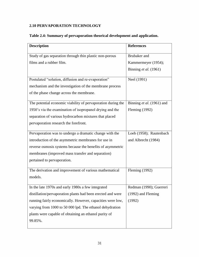
2.10 PERVAPORATION TECHNOLOGY
Table 2.4: Summary of pervaporation theorical development and application.
Description References
Study of gas separation through thin plastic non-porous
films and a rubber film.
Brubaker and
Kammermeyer (1954);
Binning et al. (1961)
Postulated “solution, diffusion and re-evaporation”
mechanism and the investigation of the membrane process
of the phase change across the membrane.
Neel (1991)
The potential economic viability of pervaporation during the
1950‟s via the examination of isopropanol drying and the
separation of various hydrocarbon mixtures that placed
pervaporation research the forefront.
Binning et al. (1961) and
Fleming (1992)
Pervaporation was to undergo a dramatic change with the
introduction of the asymmetric membranes for use in
reverse osmosis systems because the benefits of asymmetric
membranes (improved mass transfer and separation)
pertained to pervaporation.
Loeb (1958); Rautenbach
and Albrecht (1984)
The derivation and improvement of various mathematical
models.
Fleming (1992)
In the late 1970s and early 1980s a few integrated
distillation/pervaporation plants had been erected and were
running fairly economically. However, capacities were low,
varying from 1000 to 50 000 lpd. The ethanol dehydration
plants were capable of obtaining an ethanol purity of
99.85%.
Redman (1990); Guerreri
(1992) and Fleming
(1992)
32
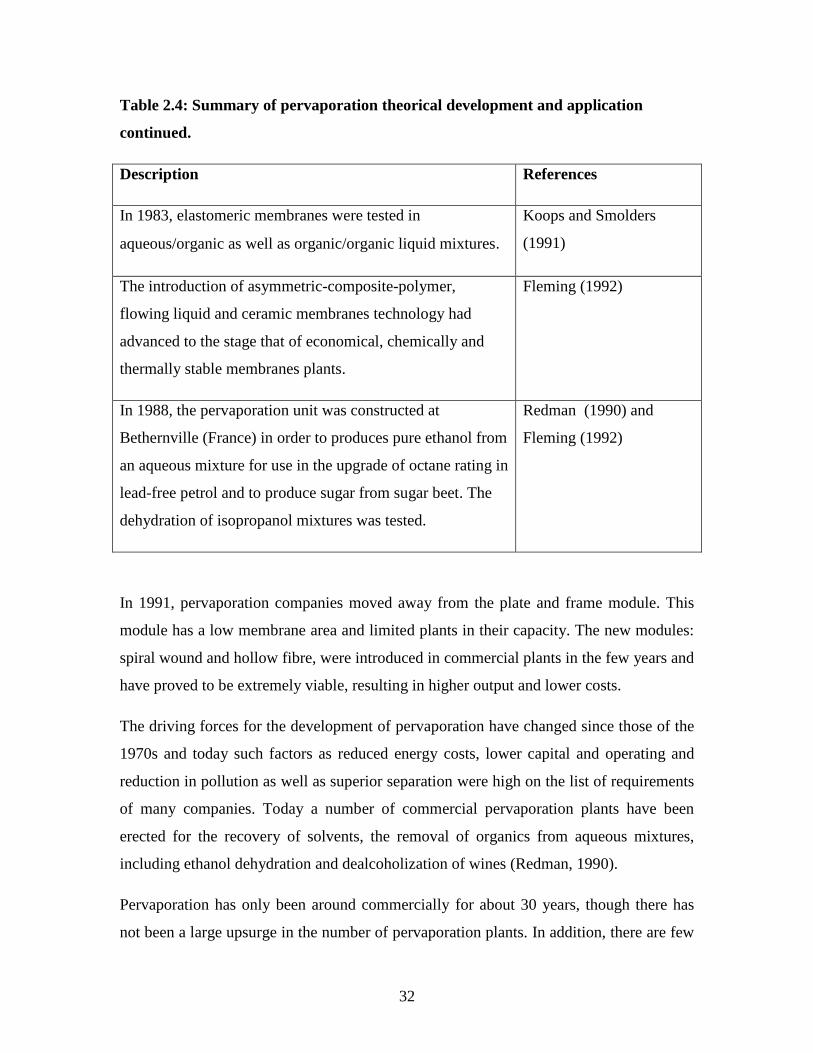
Table 2.4: Summary of pervaporation theorical development and application
continued.
Description References
In 1983, elastomeric membranes were tested in
aqueous/organic as well as organic/organic liquid mixtures.
Koops and Smolders
(1991)
The introduction of asymmetric-composite-polymer,
flowing liquid and ceramic membranes technology had
advanced to the stage that of economical, chemically and
thermally stable membranes plants.
Fleming (1992)
In 1988, the pervaporation unit was constructed at
Bethernville (France) in order to produces pure ethanol from
an aqueous mixture for use in the upgrade of octane rating in
lead-free petrol and to produce sugar from sugar beet. The
dehydration of isopropanol mixtures was tested.
Redman (1990) and
Fleming (1992)
In 1991, pervaporation companies moved away from the plate and frame module. This
module has a low membrane area and limited plants in their capacity. The new modules:
spiral wound and hollow fibre, were introduced in commercial plants in the few years and
have proved to be extremely viable, resulting in higher output and lower costs.
The driving forces for the development of pervaporation have changed since those of the
1970s and today such factors as reduced energy costs, lower capital and operating and
reduction in pollution as well as superior separation were high on the list of requirements
of many companies. Today a number of commercial pervaporation plants have been
erected for the recovery of solvents, the removal of organics from aqueous mixtures,
including ethanol dehydration and dealcoholization of wines (Redman, 1990).
Pervaporation has only been around commercially for about 30 years, though there has
not been a large upsurge in the number of pervaporation plants. In addition, there are few
33
companies involved in the production of the membranes themselves, but this will
hopefully change in the future as the demand increases. Haggin (1988) predicted that
membrane growth will be somewhere in the region of 12 to 14% annually as from 1990,
however, the growth may be stifled if the technical and economic problems concerning
membrane systems are not reduced. A factor affecting the successful introduction of
pervaporation into industry is the low fluxes which are presently achieved. The low flux
does not compare favourably with mass flow rates that alternative unit operations can
produce. However, with the advent of high area/module volume ratio (high packing
density) systems, pervaporation should find an increased usage within industrial
applications. Generally industrial pervaporation plants require hollow fibre pervaporation
modules for increased mass flow rate while laboratory scale units use plate and frame
modules because of their ease of operation on a small scale.
The most advances in pervaporation researches have been done in the past 20 to 30 years
as new polymers have been synthesized and as the theory of sorption and diffusion in
polymers has been improved (Yamposki and Volkov, 1991). Improvement in both
hydrophobic and hydrophilic membranes (Driolli, 1992) via cross linking using
composite membranes makes pervaporation more inviting as time progresses. The future
prospects for pervaporation, as well as with other membrane processes, rely on continued
research into the chemistry of the polymer. The separation of organic mixtures and
ethanol-water mixture using pervaporation looks set to be an important field of the future.
The United States Department of Energy (DoE) ranks this particular pervaporation area
as its top research priority (Haggin, 1990). Though there have been numerous
investigations conducted on the pervaporative separations of organic/organic mixtures
and liquid mixtures, there are no large scale pervaporation plants dealing with the
separation of alcohol and water, only medium scale plants are in operation. It would
appear that the current application of pervaporation industrially, that is the dehydration of
alcohols, will continue increasing, using different types of pervaporation membranes.
Theory of pervaporation membrane
In principle, pervaporation is based on the solution-diffusion mechanism. Its driving
force is the gradient of the chemical potential between the feed and the permeate sides of
34
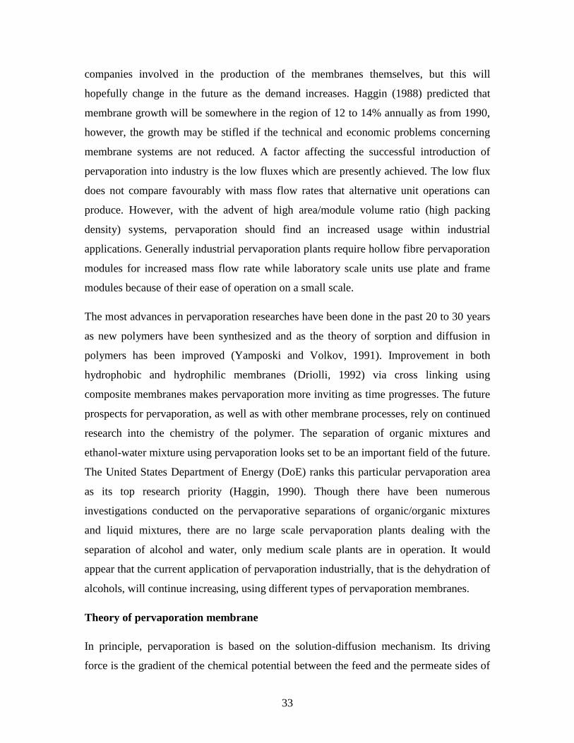
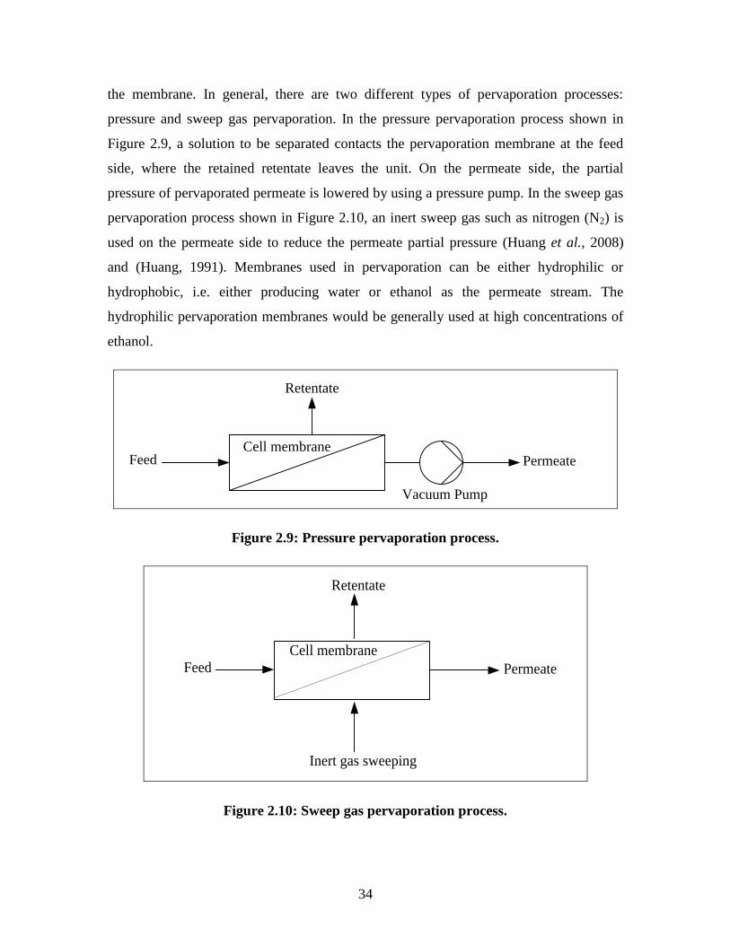
the membrane. In general, there are two different types of pervaporation processes:
pressure and sweep gas pervaporation. In the pressure pervaporation process shown in
Figure 2.9, a solution to be separated contacts the pervaporation membrane at the feed
side, where the retained retentate leaves the unit. On the permeate side, the partial
pressure of pervaporated permeate is lowered by using a pressure pump. In the sweep gas
pervaporation process shown in Figure 2.10, an inert sweep gas such as nitrogen (N2) is
used on the permeate side to reduce the permeate partial pressure (Huang et al., 2008)
and (Huang, 1991). Membranes used in pervaporation can be either hydrophilic or
hydrophobic, i.e. either producing water or ethanol as the permeate stream. The
hydrophilic pervaporation membranes would be generally used at high concentrations of
ethanol.
Feed
Retentate
Vacuum Pump
PermeateCell membrane
Figure 2.9: Pressure pervaporation process.
Permeate
Retentate
Inert gas sweeping
Cell membrane
Feed
Figure 2.10: Sweep gas pervaporation process.
35
The hydrophilic membranes are available as inorganic membrane or polymeric
membranes. Inorganic membranes exhibit greater temperature stability and mechanical
strength and they are expensive. An expensive type of inorganic pervaporation
membranes are tubular zeolite NaA and silica membrane. The tubular zeolite NaA
membrane module, has a pervaporation flux of 2.35 kg/m2h and the separation factor of
above 5000 for the solution of 95 wt% ethanol at 368.15 K (Busca et al., 2008). The NaA
zeolite membrane showed high water selectivity permeation and high permeation flux
(Busca et al., 2008 and Huang et al., 2008).
The polymeric membranes are commonly used materials for membranes. The advantages
of polymeric pervaporation membranes are low energy and material consumption, the
continuous character of the processes simplicity, and flexibility of control. However,
upon wetting, they swell altering the structure of the membrane (Verhoef et al., 2008).
Swelling occurs because a solvent enters and passes through the membrane, due to a
chemical potential gradient. This increases the permeability. The advantage of combining
inorganic membrane and polymeric membrane is to obtain the high ratio of membrane
performance. A large number of polymeric pervaporation membranes, for example
cellulose acetate butyrate membrane, polydimethylsiloxane (PDMS) membrane,
polydimethysiloxane-polystyrene interpenetrating polymer network (PDMS-PS IPN)
supported membranes, aromatic polyetherimide membranes have been investigated.
According to Busca et al. (2008) and Huang et al. (2008) the preferable membrane is a
PDMS membrane as a continuous fermentation/membrane pervaporation system to
produce ethanol resulting in permeates of 20 – 23 wt% while 4 – 6 wt% level was
retained in stirred tank fermentor. The selectivity ranged from 1.8 to 4.1 when using
polydimethysiloxane-polystyrene interpenetrating polymer network supported
membranes for pervaporation separation of ethanol from aqueous solutions (Huang et al.,
2008). For the feed having low ethanol concentration the membrane was more selective
for ethanol, at high ethanol concentrations it was more selective for water. Huang et al.
(2008) investigated the sorption, diffusion and pervaporation of ethanol solution in
homogeneous and composite aromatic polyetherimide membranes. The performance of
these membranes was found dependent on the permeate diffusivity rather than its
solubility.
36
2.11 PERVAPORATION PROCESS
Characteristics of the pervaporation membrane
The pervaporation process offers several distinguishing characteristics:
Direct separation of azeotropic and close boiling mixtures
It has low energy consumption when compared to other liquid mixture separation
techniques
No solvent required, no contamination
Permeate must be volatile at operating conditions
Its functioning is independent of vapour-liquid equilibrium
Although pervaporation and vapour permeation are attractive membrane separation
technologies, they are quite often combined with distillation, leading to unrivalled
performance when compared to each respective technology alone.
Pervaporation membranes used for ethanol mixture
Based on the materials used for membrane production, there are three categories of
membranes: inorganic, polymeric and composite membrane.
Inorganic membrane
Inorganic pervaporation membranes have more popular applications in chemical reaction,
because of their superior temperature stability and mechanical strength (Sommer and
Melin, 2000). For example, tubular zeolite NaA and silica membranes are still stable at
temperature of above 573.15 K and feed pressures above 100 bar.
Polymeric membrane
According to O‟Brien and Craig, (1996), the preferable membrane is PDMS membrane
as a continuous fermentation/membrane pervaporation system to produce ethanol. It
results in permeates of 20 – 23 wt% while 4 – 6 wt% level were retained in stirred tank
fermentor. The selectivity ranged from 1.8 to 4.1. Schue et al. (1999) investigated the
sorption, diffusion and pervaporation of the ethanol solution in homogeneous and
37
composite aromatic polyetherimide membranes. The performance of these membranes
was found dependent on the permeate diffusivity rather than its solubility.
Composite or mixed membrane
To combine the advantages of inorganic membrane and polymeric membranes and obtain
high ratio of membrane performance, various inorganic-polymer or polymer-polymer
composite membranes such as polystyrenesulfonate/alumina, poly-electrolytes multi-
layer mixed matrix membranes and poly-sodium alginate blend membranes have been
studied for pervaporation separation of the ethanol/water mixture (Dong et al., 2006).
They prepare a hollow fiber composite membrane PVA-SA blend, supported by a
polysulfone (PS) hollow-fiber ultrafiltration membrane for pervaporation ethanol
dehydration. With ethanol concentration at 90 wt% in the feed at 318.15 K the separation
factors of 384 and permeation fluxes of 384 g.m-2
.h-1
were obtained (Dong et al., 2006).
Pervaporation of aqueous organic mixtures
Pervaporation of aqueous mixtures is an extremely important research area in
pervaporation technology as it is the most widely researched field (Dutta and Sikdar,
1991) and the only field to date that has been scaled successfully to industrial scale. Most
of the mathematical models have been derived using these particular mixtures, and the
mathematical models hold for under trial scale organic/organic pervaporation as well.
The system of ethanol/water dehydration system has gained more attention in research.
The ethanol/water mixture was tested for its solubility and permeability characteristics in
different membranes (Mulder et al., 1985). One common feature, except in the
water/ethanol/polysulfone data, is that sorption into the membrane is a rate controlling
factor in the mechanism of these particular pervaporations. However, the polysulfone
membrane shows the diffusion through the membrane to be rate controlling.
An integrated pervaporation/fractional distillation system was explored as a possible
avenue for the purification of ethyl alcohol (Guerreri, 1992). It was found that
pervaporation with a PVA/PAN composite membrane provided a high driving force for
ethanol dehydration and that separation purities after the pervaporation step were well
38
above that of the azeotropic concentration of 95.57 wt% (at atmosphere pressure). In fact
purities of 99.85 wt% were attainable. Guerreri (1992) believed that using an integrated
pervaporation/distillation system, one could reduce capital and operating costs by
approximately 25%. Guerreri (1992) also proposed a mathematical model similar to that
derived by Rautenbach and Albrecht (1980).
Separation factors as high as 900 and flux of 1 kg/m2.h were reported (Nakane and
Yanagishita, 1992) when using an asymmetric polyimide membrane to concentrate
aqueous ethanol mixtures. The separation factor is an expression defined in a similar
manner to the selectivity that describes the performance of the system in separating
mixtures.
Four different membranes: silicone composite; polydimethylsiloxane (PDMS);
polymethyoxysilone (PMS) and polyether block amide (PEBA), were used to
concentrated acetone-water mixtures using the pervaporation process (Hollein et al.,
1993). Fluxes were generally low (less than one kg/m2.h and selectivities were higher
(greater than 30) – expect for the PMS and PEBA membranes, where selectivities were
below ten. The PEBA membrane, tested by Hollein et al. (1993), was inefficient for their
particular system while the silicone composite gave the best results and was then used to
test temperature and pressure effects.
Raghunath and Hwang (1992) looked at aqueous toluene and aqueous phenol separation
through PDMS and PEBA membranes. Increasing membrane thickness had a pronounced
effect on decreasing the flux of both aqueous mixtures as is expected when using Fick‟s
law to describe the mass transport. Increases in membrane thickness also resulted in
decreases in the selectivity of the organic component from water, though from the
definition of selectivities, it is not obvious why there should be any effect of the
membrane thickness on the selectivity.
Rautenbach and Albrecth (1984) studied the water/isopropanol/cellulose system. Both
asymmetric and symmetric membranes were modeled mathematically. Flux increased
with increasing water content in the feed while separation was achieved. The reduction in
flux with increasing membrane thickness was also noted (Rautenbach and Albrecht,
39
1984). They also noted the presence of a temperature drop across the membrane and
recorded the drops until the temperature reach 278.15 K. This temperature drop is often
assumed negligible, yet for accurate modeling, it should be taken into account. The
temperature drop cannot be predicted by the model unless heat transfer effects describing
the loss of energy in vapourising component are included within the model.
Rautenbach et al. (1988) measured the water/isopropanol system using PVA/PAN
membrane. Flux varied linearly with water concentration and followed Arrhenius law
with respect to temperature. Excellent separation was achieved, decreasing with
increasing water content and unaffected by temperature changes. These results were in
agreement with those found by Mulder et al. (1985). `
Boddeker et al. (1990) selected the polyether-polyamide block copolymer (PEBA) via a
screening process conducted with three different membranes, for separating various
aqueous butanol isomers. Organic flux density through the PEBA membranes increased
dramatically after 3 wt% butanol in the feed had been reached, however, for the butanol
isomer, 2-methyl-2-propanol, a small increase in flux with increasing feed concentrated
was noted. Increasing permeate pressure (downstream pressure) resulted in a decrease in
flux as the saturation pressure had been reached.
Separation of alcohol and water by pervaporation membrane
Pervaporation is the recent technology used as the removal of organic from water (Peng
et al., 2003). Pervaporation membranes separate water at the feed side and a vapour at the
permeate side, simultaneously evaporating the permeating compound. The polyether-
polyamide block copolymer (PEBA) membrane is used for the separation of aromatics,
and it was found that it was suitable for the separation of phenol and water (Kondo and
Sato, 1994).
The separation of a phenol/water mixture using a polyurethane membrane by a
pervaporation method was investigated by Hoshi et al. (1997). The polyurethane layer
was sandwiched within a porous polypropylene membrane. Pervaporation measurement
was carried out under pressure on the permeate side and the permeate vapour was
collected with a liquid nitrogen trap. The phenol concentration in the permeate solution
40
increased from 0 to 65 wt% with increasing the feed concentration of phenol from 0 to 7
wt%. The total flux increased up to 930 g/m2.h with increasing phenol partial flux. In the
sorption membrane at 333.15 K, the concentration of phenol in the membrane was 68
wt% which was higher than that of the permeate solution. Therefore, it was considered
that the phenol selectivity was based on high solubility in the polyurethane membranes.
Application of the pervaporation for the removal of phenol from water solutions
modeling wastewater was investigated (Kujawski and Pozniak, 2004) using the following
composite membranes: PEBA, polydimethylsiloxane (PDMS) and zeolite –filled PDMS
pervaporation. It was found that the PEBA membrane achieved the best selectivity.
Field and Lobo (2002) have reported that the pollution control was achieved and waste
minimised. It was found that pervaporation is more viable when operated as a
pervaporation-decanter hybrid process than in a stand-alone mode.
Xu et al. (2006) studied twelve kinds of polyimide membranes for separation of ethanol
and water mixtures for pervaporation properties. Twelve kinds of polyimide membranes
using three dianhydrided (including 2,2-bis[4-(3,4-dicarbonxyphenoxy)phenyl]propane
dianhydride (BPADA), 3,3,4,4-benzophenonetetracarboxylic dianhydride (BTDA), and
3,3,4,4-biphenyltetracarboxylic dianhdride (ODPA) and four diamines (including
benzidine (BZD), bis(4-aminophenyl)phenyl phosphate (BAPP), 4,4-
diaminodiphenylmethane (MDA), and 4,4- diaminodiphenylether (ODA) consist of two
steps. The permeation experiments of water + ethanol mixtures through 12 polyimide
membranes were carried out at 333.15 K. The temperature dependence of pervaporation
performances on ODA-based polyimide membranes were investigated. The flux of
ethanol + water mixtures through the polyimide membranes with the same dianhydrides
increased following the order of BZD < ODA < MDA < BAPP. The permeation flux
increases with an increase in temperature and the relationship between the flux and
temperature can be described by the Arrhenius equation.
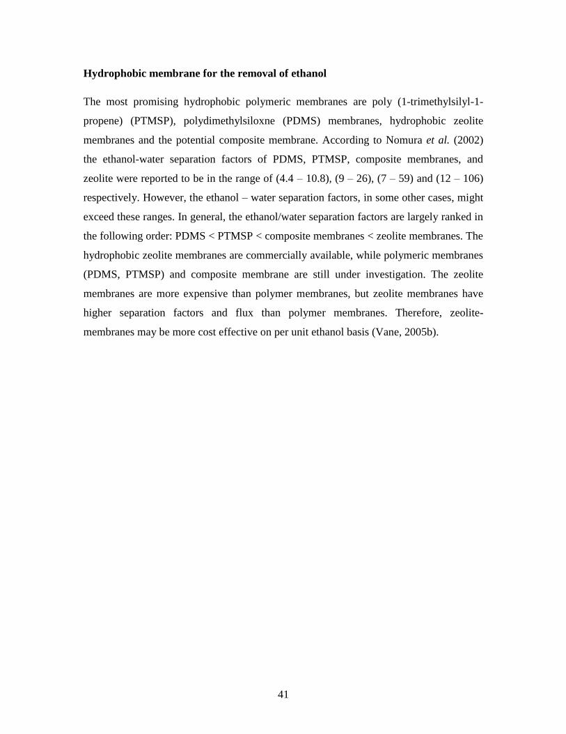
41
Hydrophobic membrane for the removal of ethanol
The most promising hydrophobic polymeric membranes are poly (1-trimethylsilyl-1-
propene) (PTMSP), polydimethylsiloxne (PDMS) membranes, hydrophobic zeolite
membranes and the potential composite membrane. According to Nomura et al. (2002)
the ethanol-water separation factors of PDMS, PTMSP, composite membranes, and
zeolite were reported to be in the range of (4.4 – 10.8), (9 – 26), (7 – 59) and (12 – 106)
respectively. However, the ethanol – water separation factors, in some other cases, might
exceed these ranges. In general, the ethanol/water separation factors are largely ranked in
the following order: PDMS < PTMSP < composite membranes < zeolite membranes. The
hydrophobic zeolite membranes are commercially available, while polymeric membranes
(PDMS, PTMSP) and composite membrane are still under investigation. The zeolite
membranes are more expensive than polymer membranes, but zeolite membranes have
higher separation factors and flux than polymer membranes. Therefore, zeolite-
membranes may be more cost effective on per unit ethanol basis (Vane, 2005b).
42
Membrane Cell
Retentate
Flow meter
P2
Chilling water in
Vacuum
Flask
Vacuum
pump
Permeate Storage
Tank
T2
Chilling water out
Cooler
Feed pump
Filter
Storage Feed
Tank
Heating
coil
T1
P1
Tank
feeder
Figure 2.11: Schematic diagram of the pervaporation set-up.
P = Pressure
T = Temperature
43
Testing of the various parameters
The testing of the various parameters are important in determining the optimal operating
conditions for pervaporation. Watson and Payne (1990) concluded in their study on the
dehydration of dilute alcohol through PDMS films. Their observations include:
As the number of carbon atoms is increased separation becomes more effective for
aqueous/organic mixtures. A similar phenomenon was discovered by (Huang and
Jarvis, 1970) with their study on low carbon aqueous alcohol pervaporation through
cellophane and PVA. Huang and Jarvis (1970) also noted that permeation rates
decreased for increasing molecular length. Lee et al. (1994) have showed similar
tested results in tests conducted on the same systems, but also noted that sorption
increased with increasing carbon content.
The selectivity declines exponentially with increasing alcohol feed content.
Separation is not always independent of membrane thickness (Raghunath and Huang,
1992).
Temperature effects might be expected due to the temperature dependent terms
solubility and diffusivity, however, the effect of temperature on separation is little or
non-existent.
Finally, sorption or solubility is the salient feature in the separation performance of
pervaporation, often dominating the diffusion process completely. Yuzhong et al.
(1993), conclude that diffusion is as important as sorption in affecting the flux but
agrees that sorption is the dominating mechanism when it comes to selectivity. Lee et
al. (1994) found that smaller alcohols were diffusivity dominant while larger alcohols
were preferentially sorbed.

44
Effect of parameters
Temperature:
Flux
With increases in temperature there is a corresponding increase in the permeate
rate. Most researchers have found that this relationship follows an Arrhenius
pattern, confirming the predictions obtained from the conceptual model (Lund,
1995).
Selectivity
The research has been conflicting. Most investigators found that there was either
no effect or the selectivity decreased slightly with increased temperature.
Increased temperature causes the membrane to become more plasticized, thus its
ability to distinguish between molecules of similar size and shape is diminished.
However, McCandless (1973) has reported a contradictory increase in selectivity
with increasing temperature and attributed it to increases in sorption with
temperature increases. Therefore, it is clear that the selectivity is not an intrinsic
property, but rather one which depends on the interaction between the
components themselves and the interaction between the components in the feed
and the membrane.
Concentration:
Flux
Most articles found that flux increase with increase concentrations of the
permeant in the feed, yet there are a few reports which have shown the opposite
relationship (McCandless et al., 1974 and Wessling et al., 1991).
Selectivity
From the literature it is apparent that selectivity decreases with increased
permeant feed concentration. Wesslein et al. (1990) however, showed that this is

45
not a “hard and fast rule” as it depends on the feed mixture and
component/membrane interactions.
Permeate pressure:
Flux
Flux was found to decrease with increased permeate pressure although if the
permeate pressure is maintained far below that of the saturation pressure, no
effect was found (Dutta and Sikdar, 1991 and Binning et al., 1961).
Selectivity
Most researchers found decreases in selectivity with increased permeate pressure.
Dutta and Sikdar (1991) found no effectof such behaviour in their investigations.
46
CHAPTER 3
THERMODYNAMIC FUNDAMENTALS
3.1 Introduction
The thermodynamic fundamentals are described and a discussion on extractive
distillation and pervaporation processes are presented. Chou and Tanioka (1999)
modified the Wilson model (1964) for data reduction schemes to predict the effect of salt
on the behavior of alcohol/water system. The VLE data reduction using the liquid phase
activity coefficient models such as Margules, Wilson, NRTL, Van Laar, UNIQUAC are
also presented. Many references such as (Wilson, 1964); (Renon and Prausnitz, 1968);
(Abrams and Prausnitz, 1975); (Smith and Van Ness, 1987); (Prausnitz et al., 1986);
(Malanowski and Anderko, 1992); (Walas, 1985); (Raal and Mühlbauer, 1998) gives
excellent and detailed coverage of thermodynamic fundamentals, and it is not the purpose
of this report to provide details coverage of the above thermodynamic fundamentals. The
pervaporation equations developed by Baker (2004) was presented in order to understand
the pervaporation principles.
47
3.2 Vapour Liquid Equilibrium System
The application of fundamental thermodynamic concepts to the problem of describing
and interpreting multicomponent phase equilibria is particularly impressive (Smith et al.,
2001). The vapour-liquid equilibrium (VLE) relations as well as other interphase
equilibrium relationships are needed in the solution of many engineering problems. The
required data can be found by experiment but such measurements are seldom easy, even
for binary systems and they become rapidly more difficult as the number of constituent
species increase. This is the incentitive for application of thermodynamics to the
calculation of phase equilibrium relationships (Smith et al., 2001)The general VLE
problem involves a multicomponent system of N constituent species for which the
independent variable are temperature, pressure and N – 1 liquid phase mole fractions and
N – 1 vapour phase mole fraction. (Note that i ix 1and i iy 1 , where xi and yi
represent liquid and vapour mole fractions respectively). There are 2N independent
variable, and applications of the phase rule shows exactly N of these variable must be
fixed to establish the intensive state of the system. The fundamental equation of phase
equilibrium based on the chemical potentials (μi) for phases and :
i i i N ( , , ...... )1 2 3 (3.1)
One can write the general expression for VLE by applying the defining relations. At
equilibrium the fugacity of the species i in the vapour and liquid phase are equal:
f fi i
(3.2)
or
f fi
v
i
l (3.3)
where: v is vapour phase and l is liquid phase
48
The definition of fugacity is completed by setting the ideal gas state fugacity of pure
species i equal to its pressure. Consider the liquid and vapour phases and their fugacity
can be expressed as follows:
f y Pi
v
i i (3.4)
dPv
RTpxf l
j
sat
i
sat
iii
l
i
1expˆ (3.5)
at equilibrium leads to
dPv
RTpxPy l
j
sat
i
sat
iiiii
1expˆ (3.6)
3.3 Fugacity Coefficient
The fugacity coefficient may be evaluated from the compressibility factor (Z) and can be
evaluated in two ways either from PVT data or obtained analytically from equations of
state (EoS).
The two term virial equation of state is given by
RT
BPZ 1 (3.7)
where B is the second virial coefficient.
The generalised correlation of the compressibility factor given by Pitzer et al., (1955) is
applicable to all gases and is given below
10 ZZZ (3.8)
Where Z0 and Z
1are both function of Tr and Pr and ω is the acentric factor.
49
The virial equation of state was used in the determination of the fugacity coefficients for
isobaric data presented in this investigation. The details and derivation of this equation of
state are presented in Smith et al. (2001). Presented below are the final equations and the
Pitzer correlation. The fugacity coefficient for a binary mixture is given by
RT
PyPPVB ijj
sat
i
l
iii
i
2
exp (3.9)
where
jjiiijj BBBi 2 (3.10)
The fugacity coefficient can also be evaluated for a multi-component mixture. The two
term virial equation of state is applicable to pressures up to 5 bar. There are various
methods to calculate the second virial coefficients in Equation (3.7) including the Pitzer
and Curl (1957) correlation, correlation of Tsonopolous (1974); Hayden and O‟Connell
method (1975). The method described in this section is the Pitzer-type correlation as it
was employed in the calculations of second virial coefficients for isobaric data. The virial
coefficients for the Pitzer-Curl correlation can be obtained from Equation (3.7) and
Equation (3.8)
10
,
,BB
P
RTB ij
ijc
ijc
ij (3.11)
The values of B0 and B
1 are obtain from
6.1
0 422.0083.0
rTB (3.12)
and
2.4
1 172.0139.0
rTB (3.13)

50
The cross coefficient parameters Tc,ij , Pc,ij P and ωij can be calculated from the empirical
mixing rules suggested by Prausnitz et al. (1999):
)1(,,, ijjcicijc kTTT (3.14)
ijc
ijcijc
ijcV
RTZP
,
,,
, (3.15)
and
2
ji
ij
(3.16)
where
2
,,
,
jcic
ijc
ZZZ
(3.17)
and
3
3/13/1
,2
ji
ijc
VcVcV (3.18)
The parameter kij in Equation (3.14) is an empirical binary interaction parameter. When
species i and j are very similar in size and chemical nature, kij is set to a value of zero.
Tarakad and Danner (1977) provide guidelines for the estimation of kij when species i and
j are not similar in size or chemical nature.
3.4 Activity Coefficient
The definition was given by the relation between the activity coefficient and the liquid
phase fugacity which is:
i
i
l
i i
f
x f
(3.19)

51
According to Gess et al. (1991), in order to obtain some physical sense of the activity
coefficient, the concept of the properties which describe the behavior of the liquid phase,
must be introduced. Excess properties express the differences between actual property
values of a solution and the values that would be exhibited by an ideal solution at the
same temperature, pressure and composition. The significance of these excess
thermodynamic properties was summarized by Wisniak and Tamir (1978) as the excess
properties
Provide key values for calculation of multicomponent mixture properties from pure
component data.
Used to define the various kinds of solutions.
Used in testing solution theories.
Provide data for evaluation of parameters characterizing interactions between unlike
species in a mixture.
The excess Gibbs energy, GE, is one of the most useful thermodynamic concepts for
expressing non-ideality of liquid mixture.
GE is the most useful quantity for determining phase stability and phase separation.
The excess enthalpy or heat of mixing, HE, is a very useful quantity in predicting
isothermal VLE and testing the thermodynamic consistency of isobaric VLE data.
The equation inter-relating these properties is known as the fundamental excess property
relation, which was derived by Van Ness (1959):
d nG
RT
nV
RTdP
nH
RTdT dn
E E E
j j
2 ln (3.20)
GE is the molar excess Gibbs energy, V
E is the molar excess volume and H
E is the molar
excess enthalpy or the heat of mixing. The implicit in equation (3.20) is the relation:
ln
, ,
i
i
T P n
GERT
n
j i
(3.21)
52
The relationship between the excess Gibbs energy and the activity coefficient can also be
expressed as:
G
RTx
E
i i ln (3.22)
Based on equations (3.22) and (3.20) the following equations can be obtained for the
activity coefficients in binary system:
1 2
1
exp
G
RTx
d GRT
dx
E
E
(3.23)
2 1
1
exp
G
RTx
d GRT
dx
E
E
(3.24)
The molar excess Gibbs energy is function of the measurable quantities temperature,
pressure and composition. Thus, it is through this excess property that the activity
coefficient can be related to these experimental quantities. According to Prausnitz et al.
(1986), at low to moderate pressures, activity coefficients are weakly dependent on
pressure and therefore their dependence is primary on temperature and composition.
Another thermodynamically important relation, which clearly shows the dependence of
the activity coefficient on the excess properties is the Gibbs-Duhem equation is:
x dV
RTdP
H
RTdTi i
E E
ln 2 (3.25)
Equation 3.25 also forms the basis of thermodynamic consistency tests. It is interesting to
note that at constant temperature and constant pressure, equation (3.25) reduces to:
x di iln 0 (3.26)
The Gibbs-Duhem equation finds an important application in thermodynamic consistency
testing of VLE data, (refer to section 3.10).
53
3.5 Activity Coefficient at Infinite Dilution
In the dilute regions some of the greatest departures from ideality are frequently observed
and consequently activity coefficients at infinite dilution are significant importance. This
can be summed up in a statement by Raal and Mühlbauer (1998) that infinite dilution
activity coefficients almost always represent the most accurate characterization of system
behavior in the dilute regions. Additional uses of activity coefficients at infinite dilution
include:
Screening for potential azeotropes (Palmer, 2000)
Screening of solvents for solvent extraction (Palmer, 2000) and extractive
distillation (Perry and Green, 2004)
Prediction of binary VLE data, which in turn are used to predict multi-component
VLE data (Howell et al., 1989)
These activity coefficients at infinite dilution can be determined experimentally by
various techniques, each having their own benefits and drawbacks. Raal and Muhlbauer
(1998), list following principal techniques:
Different ebulliometry
Use of a different dynamic or static apparatus
Gas chromatographic methods
Inert gas stripping
The prediction of activity coefficient at infinite dilution are usually performed with group
contribution models such as UNIFAC and ASOG and some correlation such as the
Margules model, Van Laar model, Wilson model, T-K-Wilson model or modified Wilson
model, NRTL model, UNIQUAC model (Walas, 1985).
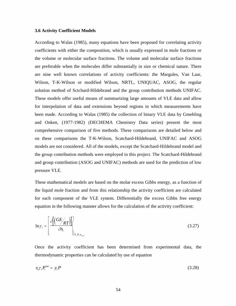
54
3.6 Activity Coefficient Models
According to Walas (1985), many equations have been proposed for correlating activity
coefficients with either the composition, which is usually expressed in mole fractions or
the volume or molecular surface fractions. The volume and molecular surface fractions
are preferable when the molecules differ substantially in size or chemical nature. There
are nine well known correlations of activity coefficients: the Margules, Van Laar,
Wilson, T-K-Wilson or modified Wilson, NRTL, UNIQUAC, ASOG, the regular
solution method of Sctchard-Hildebrand and the group contribution methods UNIFAC.
These models offer useful means of summarizing large amounts of VLE data and allow
for interpolation of data and extensions beyond regions in which measurements have
been made. According to Walas (1985) the collection of binary VLE data by Gmehling
and Onken, (1977-1982) (DECHEMA Chemistry Data series) present the most
comprehensive comparison of five methods. These comparisons are detailed below and
on these comparisons the T-K-Wilson, Scatchard-Hildebrand, UNIFAC and ASOG
models are not considered. All of the models, except the Scatchard-Hildebrand model and
the group contribution methods were employed in this project. The Scatchard-Hildebrand
and group contribution (ASOG and UNIFAC) methods are used for the prediction of low
pressure VLE.
These mathematical models are based on the molar excess Gibbs energy, as a function of
the liquid mole fraction and from this relationship the activity coefficient are calculated
for each component of the VLE system. Differentially the excess Gibbs free energy
equation in the following manner allows for the calculation of the activity coefficient:
ln
, ,
i
i
T P n
GERT
n
j i
(3.27)
Once the activity coefficient has been determined from experimental data, the
thermodynamic properties can be calculated by use of equation
x P y Pi i i
sat
i (3.28)
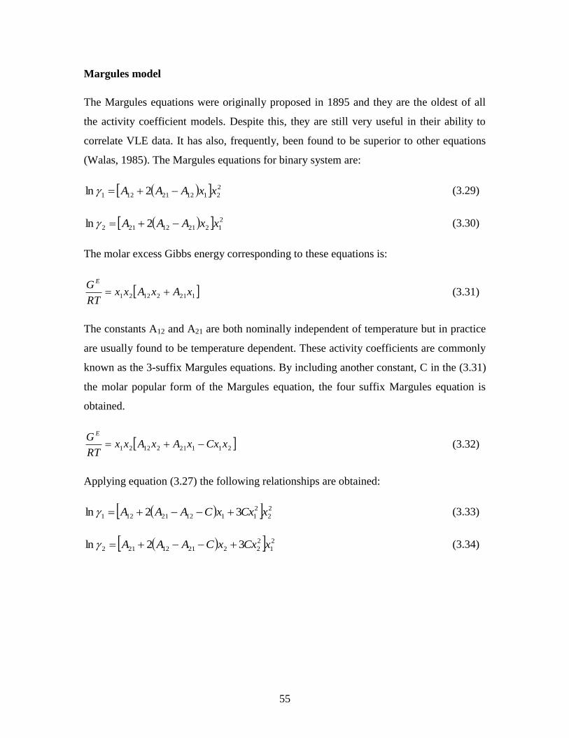
55
Margules model
The Margules equations were originally proposed in 1895 and they are the oldest of all
the activity coefficient models. Despite this, they are still very useful in their ability to
correlate VLE data. It has also, frequently, been found to be superior to other equations
(Walas, 1985). The Margules equations for binary system are:
2
211221121 2ln xxAAA (3.29)
2
122112212 2ln xxAAA (3.30)
The molar excess Gibbs energy corresponding to these equations is:
12121221 xAxAxxRT
G E
(3.31)
The constants A12 and A21 are both nominally independent of temperature but in practice
are usually found to be temperature dependent. These activity coefficients are commonly
known as the 3-suffix Margules equations. By including another constant, C in the (3.31)
the molar popular form of the Margules equation, the four suffix Margules equation is
obtained.
2112121221 xCxxAxAxxRT
G E
(3.32)
Applying equation (3.27) the following relationships are obtained:
2
2
2
111221121 32ln xCxxCAAA (3.33)
2
1
2
222112212 32ln xCxxCAAA (3.34)

56
Van Laar model: (Prausnitz et al., 1986)
This model is suitable for constituents in a binary system that are similar chemically and
have differing molar volumes. All interaction parameters except a12 are ignored. This
model has been found to represent some complex systems despite its derivation which
suggests that it is suitable for simple, non-polar liquids. The advantage of this model is
that it is mathematically simple, yet flexible. The Gibbs excess expression is as follows:
G
RT
A A x x
x A x A
E
12 21 1 2
1 12 2 21
(3.35)
ln 1 12
21 2
1 12 2 21
2
A
A x
x A x A (3.36)
ln 2 21
12 1
1 12 2 21
2
A
A x
x A x A (3.37)
The above equations take into account the size difference between molecules. However,
according to Gess et al. (1991), the Van Laar equations do not represent highly non-ideal
system well. This indicates that the interactions between molecules are not properly
characterized by this activity coefficient model. Prausnitz et al. (1986) recommend the
use of the Van Laar equations for relatively simple non-polar solutions. However, these
equations have been found to be capable of represent the activity coefficient of some
complex mixtures (Walas, 1985). According to Smith and Van Ness (1987) the Margules
and Van Laar equations are special cases of a very general treatment based on rational
functions, i.e on equation for GE given by ratios of polynomials. They have the merit of
mathematical simplicity and they provide great flexibility in the of VLE data for binary
systems. However, they have no sound theoretical foundation and there is no rational
basis for extension to multicomponent systems.
Wilson model
Wilson (1964) developed a model which was based on the concept of local composition.
Local compositions which occur within a liquid solution are different from the overall
mixture composition and are presumed to account for the short range order and non-
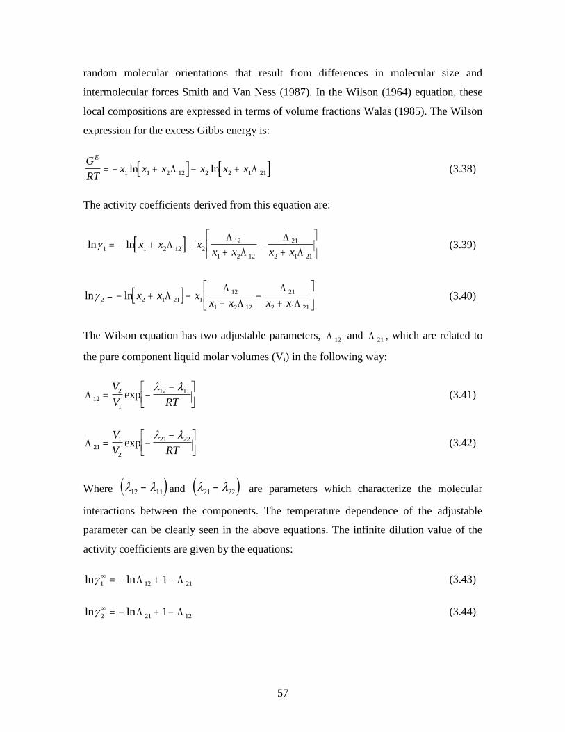
57
random molecular orientations that result from differences in molecular size and
intermolecular forces Smith and Van Ness (1987). In the Wilson (1964) equation, these
local compositions are expressed in terms of volume fractions Walas (1985). The Wilson
expression for the excess Gibbs energy is:
G
RTx x x x x x
E
1 1 2 12 2 2 1 21ln ln (3.38)
The activity coefficients derived from this equation are:
ln ln 1 1 2 12 2
12
1 2 12
21
2 1 21
x x x
x x x x
(3.39)
ln ln 2 2 1 21 1
12
1 2 12
21
2 1 21
x x x
x x x x
(3.40)
The Wilson equation has two adjustable parameters, 12 and 21 , which are related to
the pure component liquid molar volumes (Vi) in the following way:
12
2
1
12 11
V
V RTexp
(3.41)
21
1
2
21 22
V
V RTexp
(3.42)
Where 12 11 and 21 22 are parameters which characterize the molecular
interactions between the components. The temperature dependence of the adjustable
parameter can be clearly seen in the above equations. The infinite dilution value of the
activity coefficients are given by the equations:
ln ln 1 12 211 (3.43)
ln ln 2 21 121 (3.44)
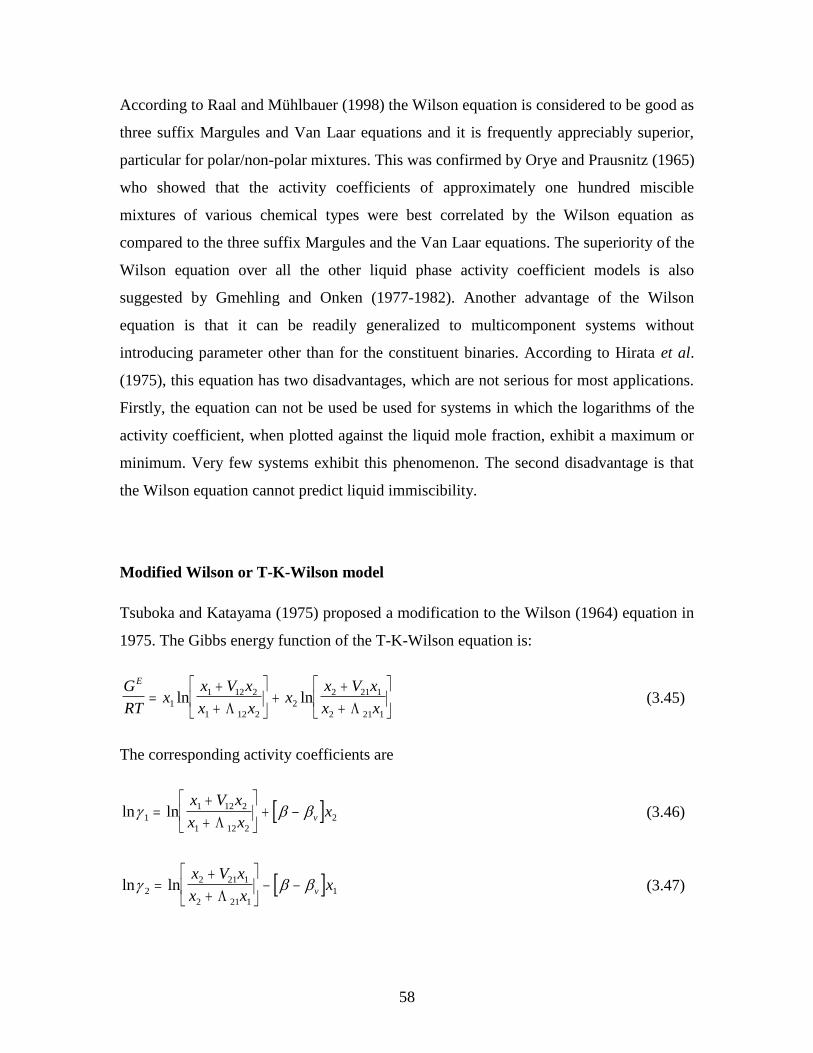
58
According to Raal and Mühlbauer (1998) the Wilson equation is considered to be good as
three suffix Margules and Van Laar equations and it is frequently appreciably superior,
particular for polar/non-polar mixtures. This was confirmed by Orye and Prausnitz (1965)
who showed that the activity coefficients of approximately one hundred miscible
mixtures of various chemical types were best correlated by the Wilson equation as
compared to the three suffix Margules and the Van Laar equations. The superiority of the
Wilson equation over all the other liquid phase activity coefficient models is also
suggested by Gmehling and Onken (1977-1982). Another advantage of the Wilson
equation is that it can be readily generalized to multicomponent systems without
introducing parameter other than for the constituent binaries. According to Hirata et al.
(1975), this equation has two disadvantages, which are not serious for most applications.
Firstly, the equation can not be used be used for systems in which the logarithms of the
activity coefficient, when plotted against the liquid mole fraction, exhibit a maximum or
minimum. Very few systems exhibit this phenomenon. The second disadvantage is that
the Wilson equation cannot predict liquid immiscibility.
Modified Wilson or T-K-Wilson model
Tsuboka and Katayama (1975) proposed a modification to the Wilson (1964) equation in
1975. The Gibbs energy function of the T-K-Wilson equation is:
G
RTx
x V x
x xx
x V x
x x
E
1
1 12 2
1 12 2
2
2 21 1
2 21 1
ln ln
(3.45)
The corresponding activity coefficients are
ln ln 1
1 12 2
1 12 2
2
x V x
x xxv
(3.46)
ln ln 2
2 21 1
2 21 1
1
x V x
x xxv
(3.47)
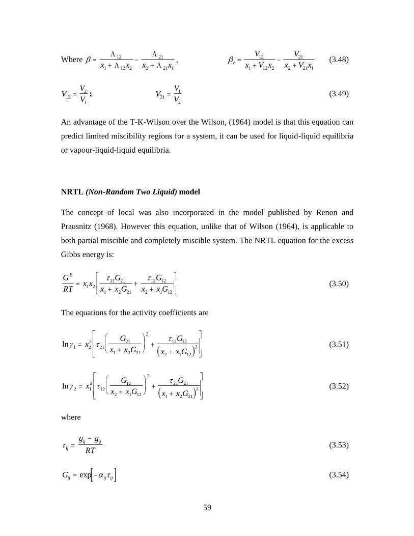
59
Where
12
1 12 2
21
2 21 1x x x x, v
V
x V x
V
x V x
12
1 12 2
21
2 21 1
(3.48)
VV
V12
2
1
; VV
V21
1
2
(3.49)
An advantage of the T-K-Wilson over the Wilson, (1964) model is that this equation can
predict limited miscibility regions for a system, it can be used for liquid-liquid equilibria
or vapour-liquid-liquid equilibria.
NRTL (Non-Random Two Liquid) model
The concept of local was also incorporated in the model published by Renon and
Prausnitz (1968). However this equation, unlike that of Wilson (1964), is applicable to
both partial miscible and completely miscible system. The NRTL equation for the excess
Gibbs energy is:
G
RTx x
G
x x G
G
x x G
E
1 2
21 21
1 2 21
12 12
2 1 12
(3.50)
The equations for the activity coefficients are
ln
1 2
2
21
21
1 2 21
2
12 12
2 1 12
2
xG
x x G
G
x x G (3.51)
ln
2 1
2
12
12
2 1 12
2
21 21
1 2 21
2
xG
x x G
G
x x G (3.52)
where
ij
ij ijg g
RT
(3.53)
Gij ij ij exp (3.54)
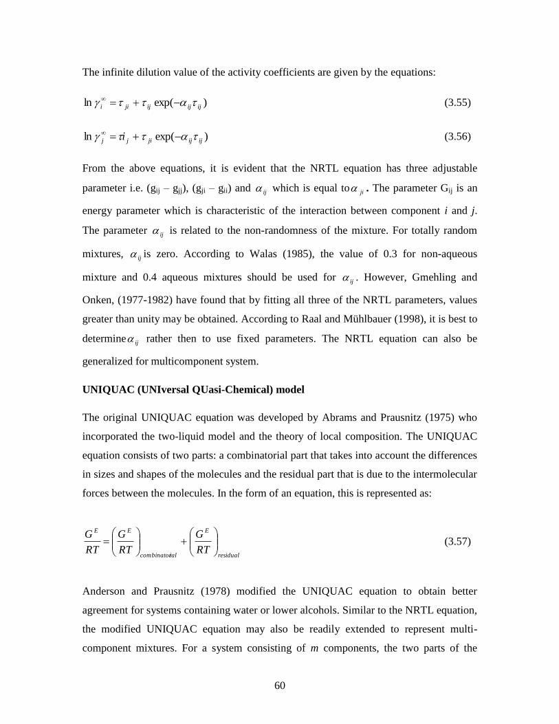
60
The infinite dilution value of the activity coefficients are given by the equations:
)exp(ln ijijijjii (3.55)
)exp(ln ijijjijj i (3.56)
From the above equations, it is evident that the NRTL equation has three adjustable
parameter i.e. (gij – gjj), (gji – gii) and ij which is equal to ji . The parameter Gij is an
energy parameter which is characteristic of the interaction between component i and j.
The parameter ij is related to the non-randomness of the mixture. For totally random
mixtures, ij is zero. According to Walas (1985), the value of 0.3 for non-aqueous
mixture and 0.4 aqueous mixtures should be used for ij . However, Gmehling and
Onken, (1977-1982) have found that by fitting all three of the NRTL parameters, values
greater than unity may be obtained. According to Raal and Mühlbauer (1998), it is best to
determine ij rather then to use fixed parameters. The NRTL equation can also be
generalized for multicomponent system.
UNIQUAC (UNIversal QUasi-Chemical) model
The original UNIQUAC equation was developed by Abrams and Prausnitz (1975) who
incorporated the two-liquid model and the theory of local composition. The UNIQUAC
equation consists of two parts: a combinatorial part that takes into account the differences
in sizes and shapes of the molecules and the residual part that is due to the intermolecular
forces between the molecules. In the form of an equation, this is represented as:
residual
E
ialcombinator
EE
RT
G
RT
G
RT
G
(3.57)
Anderson and Prausnitz (1978) modified the UNIQUAC equation to obtain better
agreement for systems containing water or lower alcohols. Similar to the NRTL equation,
the modified UNIQUAC equation may also be readily extended to represent multi-
component mixtures. For a system consisting of m components, the two parts of the
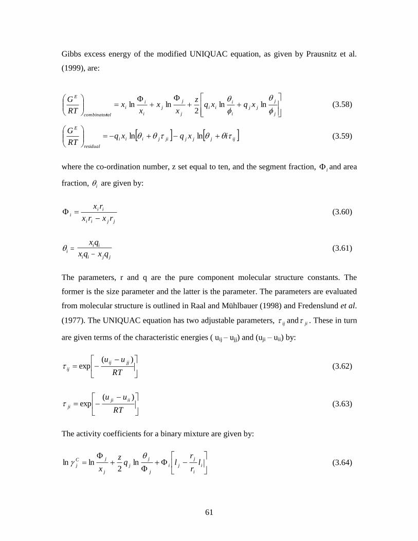
61
Gibbs excess energy of the modified UNIQUAC equation, as given by Prausnitz et al.
(1999), are:
j
j
jj
i
i
ii
j
j
j
i
i
i
ialcombinator
E
xqxqz
xx
xx
RT
G
lnln
2lnln (3.58)
ijjjjjijiii
residual
E
ixqxqRT
G
lnln (3.59)
where the co-ordination number, z set equal to ten, and the segment fraction, i and area
fraction, i are given by:
jjii
ii
irxrx
rx
(3.60)
i
i i
i i j j
x q
x q x q
(3.61)
The parameters, r and q are the pure component molecular structure constants. The
former is the size parameter and the latter is the parameter. The parameters are evaluated
from molecular structure is outlined in Raal and Mühlbauer (1998) and Fredenslund et al.
(1977). The UNIQUAC equation has two adjustable parameters, ij and ji . These in turn
are given terms of the characteristic energies ( uij – ujj) and (uji – uii) by:
RT
uu jjij
ij
)(exp (3.62)
RT
uu iiji
ji
)(exp (3.63)
The activity coefficients for a binary mixture are given by:
i
i
j
ji
j
j
j
j
jC
j lr
rlq
z
x
ln
2lnln (3.64)
62
ln ln
j
R
j i ij i j
ji
i j ji
ij
i ij
q j qj
(3.65)
where
lz
r q ri i i i 2
1 (3.66)
Abrams and Prausnitz (1975) defined the size and area parameters as the following:
rV
i
wi
0 01517. (3.67)
qA
i
wi
25 108. * (3.68)
where Vwi (m3/kmol) and Awi (m
3/kmol) are the Van der Waals volumes and areas,
respectively. A much simpler approach for the evaluation of the ri and the surface qi
parameters is achieved by obtain the parameter as the sum of the molecular structure
contributions (r and q, respectively) of the various functional groups that are present in
the molecule i.e the group contribution method (Sandler, 1999). In this method, the r and
q values of a relatively small number of functional groups or subgroups can be used to
obtain the molecular structural parameters of a huge collection of different molecular
structures involved in phase equilibrium studies.
The UNIQUAC equation is applicable to a various of liquid mixtures containing polar or
non-polar fluids. It can also be applied to multicomponent and partially miscible
mixtures. The UNIQUAC equation was slightly modified by Anderson and Prausnitz,
(1978). The aim of their modification was to improve the performance of the UNIQUAC
equation with systems containing lower alcohols or water. Anderson and Prausnitz (1978)
recommended the use of empirically adjusted values of q1 for water and lower alcohols in
the calculation of the residual term.
63
3.7 Comparison of Models Equations
According to Walas (1985) the merits of the individual activity coefficient correlation
methods have been cited locally. The comparisons of equation are summarized;
The Margules, Van Laar equations and related algebraic forms have the merit of
mathematical simplicity, ease of evaluation of the parameter from activity coefficient
data and often adequate representation of even fairly nonideal binary mixture,
including partially miscible liquid system. They are not applicable to multicomponent
system without ternary or higher interaction parameter.
The Wilson equation represents vapour liquid equilibria (VLE) of binary and
multicomponent mixtures very well with only binary parameters, because of its greater
simplicity it may be preferable to the NRTL and UNIQUAC equations for this
purpose. Although it is not directly applicable to liquid-liquid equilibria (LLE), the
equally simple T-K-Wilson equation probably is satisfactory, though it has not been
tested as thoroughly as some others. The Wilson equation is the basis of the ASOG
group contribution method for the activity coefficients.
The NRTL equation represents vapour-liquid equilibria and liquid-liquid equilibria of
the binary and multicomponent system quite well and its often superior of binary
others for aqueous systems. It is simpler in the form than the UNIQUAC method but
has the disadvantage of involving three parameters for each pair of constituents.
The UNIQUAC equation is algebraically the most complex one, although it employs
only two parameters per pairs of components. It utilizes knowledge of molecular
surfaces and volume the pure components, which can be estimated from structural
contributions and for this reason the method may be particular applicable to mixture of
widely different molecular sizes. It is applicable to vapour-liquid equilibria and liquid-
liquid equilibria of multicomponent data only. UNIQUAC is the basis of the UNIFAC
group contribution methods for activity coefficients from structure and receives much
support in the literature.

64
3.8 VLE PREDICTION OF THE ALCOHOL-WATER-SALT SYSTEM
The proposed model based on solvation between pure solvent and salt, for the prediction
of salt effect on vapour-liquid equilibria was presented by using only the vapour pressure
data of pure solvent and salt systems that compose the mixed solvent with salt system
(Ohe, 1998). The proposed models predicts thermodynamically the salt effect by
solvation number between each pure solvent and salt determined from vapour pressure
data (Ohe, 1976). In this study, the modified Wilson model was used to predict
interaction parameters for the ternary system of ethanol-water-salt (calcium chloride salt).
Modified Wilson model
According to Chou and Tanioka (1999) at low pressure, it can be assumed that the vapour
phase is ideal ( 1i ) and the activity coefficient of solvent n, n in the mixed solvent-
salt system can be expressed by
sat
nn
n
nPx
Py
(3.69)
Where yn is the mole fraction of solvent n in the vapour phase, P is the total pressure, xn
is the salt-free mole fraction of solvent n the liquid phase, and sat
nP is the saturation
vapour pressure of pure solvent n at the given system temperature.
For the binary mixture containing a dissolved salt system, the activity coefficients of the
solvents can be calculated using the modified Wilson model
2212111 lnln xxxs (3.70)
1121222 lnln xxxs (3.71)
Where
12122
21
21211
12
xxxx ss
(3.72)
65
12 and 21 are the solvent-solvent interaction parameters which are the same as those
for the original Wilson model, and 1s and 2s are the solvent-salt interaction parameter
which can be estimated by considering the ion-ion and solvent-ion interactions describe
the salting effect on the VLE (Chou and Tanioka, 1999).
For binary system of solvent-salt solution, x1 1and x2 0
Therefore equations (3.69) and (3.70) reduces to
ln ln 1 1 s (3.73)
ln ln 2 2 s (3.74)
It can also shown that at the system temperature, T, the equation (3.70) becomes
satP
P
1
1 (3.75)
Similarly for the solvent-salt solution, Ps
1
sat
s
P
P
1
1
1 (3.76)
Substituting equation (3.73) into (3.76), the solvent-salt interaction parameter is derived
as
),(
)(
11
1
1mTP
TPs
sat
s (3.79)
where m1 is the salt motility distributed in the solvent. The distribution of salt in the
mixed solvent is estimated by a simple mixing rule based on the solubility of the salt
(Chou and Tanioka, 1999).
ms x
s xm
n nn
1
1 1
(3.80)
66
where sn is the solubility of salt in solvent n, and m is the total salt molality in the ternary
system. Similarly, 2s could be obtained by the same method. At low pressures, the
vapour pressure of the alcohol-salt and water-salt solutions, Ps
1 and Ps
2 is determined
from
sat
n
bi
nn
s
n PxP (3.81)
where n = 1 or 2 and n
bi is the activity coefficient of solvent n in the binary mixture.
3.9 Low pressure VLE data reduction
There are different methods available for the regression of isothermal and isobaric VLE
data. However, only the two well-known methods were used to study the VLE data
measured for this project. The first method is known as the gamma/phi (γ-Ф) formulation
of VLE or more commonly known as the combined method, while the second method is
known as the phi/phi (Ф-Ф) method or the direct method. The combined method was
used in this work to regress the VLE data. The combined method uses an equation of
state to calculate the fugacity coefficients that describe the vapour phase nonidealities,
while an activity coefficient model is used to calculate the activity coefficients that
describe the liquid phase non-idealities. In the direct method, the fugacity coefficients are
used to describe the non-idealities in both the vapour and liquid phases and are calculated
using an equation of state.
There are different calculation procedures for each method which depend on the nature of
the VLE data. For isothermal VLE data, the pressure and vapour composition are
calculated (bubble point pressure computation), whereas for isobaric VLE data, the
temperature and vapour composition are calculated (bubble point temperature
computation) for each experimental point. Therefore, a set of data points comprising of
P-x values at a specified temperature or T-x values at a specified pressure are sufficient to
allow determination of the activity coefficient model parameters. However, (Smith et al.,
2001) encourages the measurement of the vapour phase mole fractions to allow
67
thermodynamic consistency testing, which is discussed in section 3.10. It should be noted
that the activity coefficient model parameters are temperature dependent (Walas, 1985).
The data reduction for isothermal VLE data is simple as the temperature dependence of
the model parameters can be considered insignificant and thus the model parameters can
be treated as constants. However, the temperature dependence of the model parameters is
significant for the reduction of isobaric VLE data and must therefore be taken into
account. The direct method was not used for the data regression and it is not describe in
this study, (refer to Smith et al. 2001 for the details).
The Combined (gamma/phi) method
The gamma/phi method relies upon liquid phase activity coefficient models to represent
VLE data. The model has been proposed to correlate the activity coefficients from a
relationship of the molar excess Gibbs energy, the liquid composition and temperature,
with the liquid composition expressed as a mole fraction (xi). Usually, more than one
model is used for VLE data regression, as one can determine which model provides a
better fit of the experimental data for a particular system. In this study, two well-known
models were used: the Wilson and NRTL models. In order to obtain the model
parameters, a suitable algorithm must be used for VLE regression.
The following steps were used for the regression of an isothermal set of experimental
binary VLE data using the gamma/phi method follows from Smith et al. (2001)
1. The temperature, liquid phase compositions and the pure component properties are
used as inputs for the regression. A suitable expression for the excess Gibbs energy, as a
function of composition, is then selected.
2. The parameters corresponding to the GE expression from step 1 are assigned with
reasonable estimates. The activity coefficients that correspond to the GE expression from
step 1 are then determined from Equation (3.21). The vapour phase is initially assumed
ideal and therefore the fugacity coefficients (Фi) are initially set to unity to allow an
initial calculation of the overall system pressure. The saturated pressures ( sat
iP ) are then
evaluated from a suitable vapour pressure correlation (such as the Antoine equation).
68
3. According to the law of mass conservation, Σxi = Σyi = 1, the overall system pressure
is therefore obtained from the equations
sat
iiiii PxPy (3.82)
2
222
1
111
satsat PxPxP (3.83)
4. The vapour mole fractions are then found from:
P
Pxy
i
sat
iii
i
(3.84)
5. Once the vapour mole fractions have been calculated, the fugacity coefficients are then
evaluated using a suitable equation of state for the second virial coefficients from
equation (3.85)
RT
PyPPVB ijj
sat
i
l
iii
i
2
exp (3.85)
6. The system pressure is then recalculated using Equation (3.83). The model parameters
are then optimised by employing a regression technique with a suitable objective function
that yields the best fit to the experimental P-x data for the entire composition range.
The regression procedure outlined above is the same for isobaric data with the exception
that the temperature is constant. The following equations were used:
2
PS (3.86)
where the difference between the model and experimental values is commonly termed a
residual and symbolised as δ. Other objective functions may also be used such as δy1, δγ1,
δγ2 and δ(GE/RT). However, according to Van Ness et al. (1978), equation (3.86) is at
least as good as any other and is the most simplest and direct objective function.
Furthermore, Van Ness and Abbott (1982) state that the objective function of equation
(3.86) is successful in reducing isothermal VLE data and may even be superior to any
other maximum likelihood method. Van Ness and Abbott (1982) also mention that
replacing the pressure with temperature in equation (3.86), provides the best objective
69
function for regressing isobaric VLE data. Therefore, equation (3.86) was chosen as the
objective function for regressing isothermal VLE data measured in this project.
According to Narasigadu (2006) the following researchers Marquardt (1963) and Gess et
al. (1991) have developed methods that use the objective function of equation (3.86) in
the above mentioned algorithm. However, computer software programmes such as
MATLAB (employed in this project) have built in functions that allow such calculations
to be performed with much ease. The regression procedure for isobaric and isothermal
data are summarised in Figures 3.1 and 3.2 respectively.
The vapour pressure of component j gives:
isat
j
sat
i
i
ii
sat
j
P
Px
PP
(3.87)
The summations are over all species including j, which is an arbitrarily selected species.
Once sat
iP is known, the corresponding value of T is obtained from the following
equation:
CPA
BT
sat
jj
j
ln or i
i
isat
i CPA
BT
ln (3.88)
where Ai, Bi, and Ci are Antoine constants.
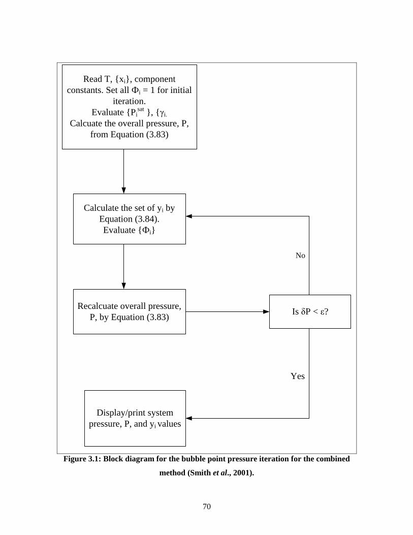
70
Read T, {xi}, component
constants. Set all Фi = 1 for initial
iteration.
Evaluate {Pisat }, {γi.
Calcuate the overall pressure, P,
from Equation (3.83)
Calculate the set of yi by
Equation (3.84).
Evaluate {Фi}
Recalcuate overall pressure,
P, by Equation (3.83)Is δP < ε?
Yes
No
Display/print system
pressure, P, and yi values
Figure 3.1: Block diagram for the bubble point pressure iteration for the combined
method (Smith et al., 2001).
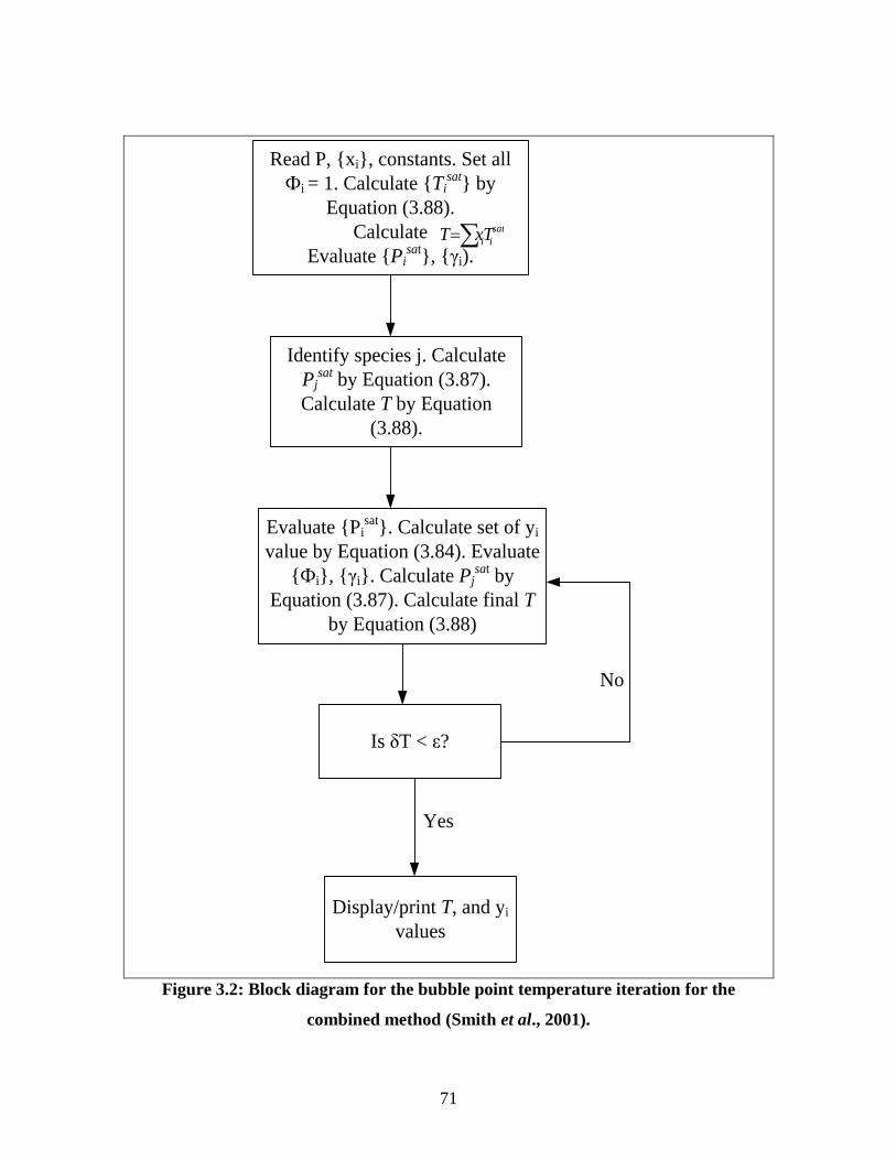
71
Read P, {xi}, constants. Set all
Фi = 1. Calculate {Tisat} by
Equation (3.88).
Calculate
Evaluate {Pisat}, {γi).
Identify species j. Calculate
Pjsat by Equation (3.87).
Calculate T by Equation
(3.88).
Evaluate {Pisat}. Calculate set of yi
value by Equation (3.84). Evaluate
{Фi}, {γi}. Calculate Pjsat by
Equation (3.87). Calculate final T
by Equation (3.88)
Display/print T, and yi
values
sat
iiTxT
Is δT < ε?
Yes
No
Figure 3.2: Block diagram for the bubble point temperature iteration for the
combined method (Smith et al., 2001).

72
3.10 Thermodynamic Consistency Test
The measurement of temperature, pressure and both liquid and vapour compositions for a
binary VLE system, results in an “over-specification” of the system. Nevertheless, this
allows one of the four measured variables to be used to test for thermodynamic
consistency. According to Smith et al. (2001), the vapour compositions usually display
the greatest error and thus the thermodynamic consistency tests usually focus on the
vapour compositions (y-data) to determine the thermodynamic consistency of the VLE
data. The Gibbs-Duhem equation forms the basis of all thermodynamic consistency tests.
dTRT
HdP
RT
Vdx
EE
ii 2ln (3.89)
At constant temperature and pressure equation (3.89) becomes
0ln ii dx (3.90)
VLE data is said to be thermodynamically consistent if it conforms to the Gibbs-Duhem
equation. Over the years, the evaluation of thermodynamic consistency of VLE data has
received a great deal of attention in the literature with many adaptations of the Gibbs-
Duhem equation being introduced. The slope test, which compared slopes of curves
drawn to fit lnγ1 and lnγ2 vs x1 graphs, was one of the earliest tests used but according to
Van Ness (1995), this test proved to be tedious and led to uncertainty. However, Walas
(1985) mentions that the area test is a necessary but insufficient condition as individual
data may be off in ways that compensate each other. For instance, the pressure is
cancelled off and hence one of the most accurately measured system properties is lost.
This means that the test would sometimes pass data sets that were inconsistent while
failing data sets that actually were consistent. Therefore, the area test was not considered
for this project but two thermodynamic consistency tests were employed: the point test of
Van Ness et al. (1973) and the direct test of Van Ness (1995). The direct test is not
discussed in this work because it was not used to test the thermodynamic consistent of
this work. A more detailed description of the direct test is provided in Van Ness (1995).
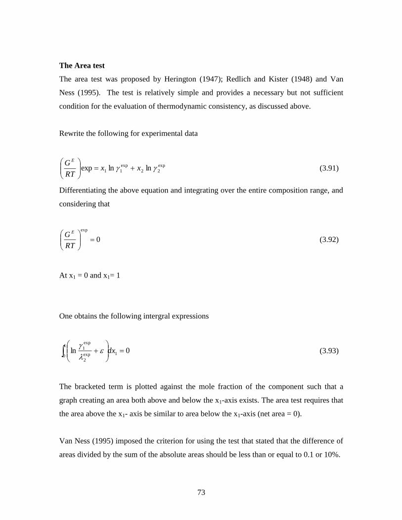
73
The Area test
The area test was proposed by Herington (1947); Redlich and Kister (1948) and Van
Ness (1995). The test is relatively simple and provides a necessary but not sufficient
condition for the evaluation of thermodynamic consistency, as discussed above.
Rewrite the following for experimental data
exp
22
exp
11 lnlnexp xxRT
G E
(3.91)
Differentiating the above equation and integrating over the entire composition range, and
considering that
0
exp
RT
G E
(3.92)
At x1 = 0 and x1= 1
One obtains the following intergral expressions
0ln 1
1
0 exp
2
exp
1
dx
(3.93)
The bracketed term is plotted against the mole fraction of the component such that a
graph creating an area both above and below the x1-axis exists. The area test requires that
the area above the x1- axis be similar to area below the x1-axis (net area = 0).
Van Ness (1995) imposed the criterion for using the test that stated that the difference of
areas divided by the sum of the absolute areas should be less than or equal to 0.1 or 10%.

74
%1021
21
aa
aa (3.94)
This is a necessary but not sufficient condition because the most important and accurately
measured variable pressure is ignored in the test due to the ratio of activity coefficients,
given below. Van Ness, 1995 also states that while the pressure can be ignored it does
however enter into the calculation of the minor factor Фi
sat
sat
sat
sat
Pxy
Pxy
Px
Py
Px
Py
1122
2211
22
22
11
11
2
1
(3.95)
According to Van Ness (1995), the area test only checks the appropriateness of the
vapour pressure ratio,
sat
sat
P
P
1
2 to the x-y data of an isothermal system.
The Point Test
Van Ness et al. (1973) introduced the point test as an improvement to the area test. Four
variables are measured for a complete binary VLE data set such as T, P, x and y. Any
three experimentally determined variables can be used to obtain the fourth variable by
employing a suitable correlation. As mentioned above, the vapour compositions introduce
the most error and are thus used to test for thermodynamic consistency. The point test
compares the measured vapour compositions (yexp) to the calculated values (ycalc), the
calculated values are found from data regression using the combined method. This
comparison generates residuals, Δy, which provides a good indication of the consistency
of the VLE data. Danner and Gess (1990) provide a quantitative criterion for the
consistency of VLE data by proposing that the absolute average deviation, Δyad, should
be less than 0.03 for the data to be thermodynamically consistent:
calcyyN
AADy exp
1)( (3.96)
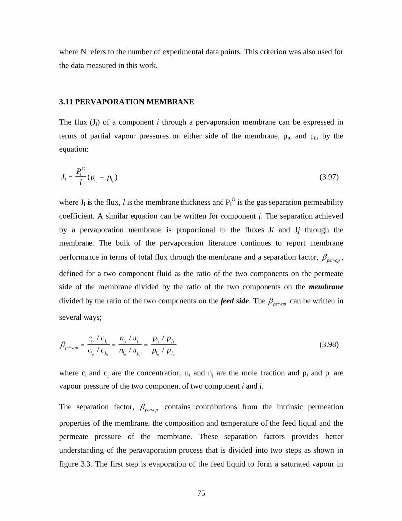
75
where N refers to the number of experimental data points. This criterion was also used for
the data measured in this work.
3.11 PERVAPORATION MEMBRANE
The flux (Ji) of a component i through a pervaporation membrane can be expressed in
terms of partial vapour pressures on either side of the membrane, pio and pil, by the
equation:
JP
lp pi
i
G
i io l ( ) (3.97)
where Ji is the flux, l is the membrane thickness and PiG is the gas separation permeability
coefficient. A similar equation can be written for component j. The separation achieved
by a pervaporation membrane is proportional to the fluxes Ji and Jj through the
membrane. The bulk of the pervaporation literature continues to report membrane
performance in terms of total flux through the membrane and a separation factor, pervap ,
defined for a two component fluid as the ratio of the two components on the permeate
side of the membrane divided by the ratio of the two components on the membrane
divided by the ratio of the two components on the feed side. The pervap can be written in
several ways;
pervap
i j
i j
i l j
i j
i j
i j
c c
c c
n n
n n
p p
p pl l
o o
l
o o
l l
o o
/
/
/
/
/
/ (3.98)
where ci and cj are the concentration, ni and nj are the mole fraction and pi and pj are
vapour pressure of the two component of two component i and j.
The separation factor, pervap contains contributions from the intrinsic permeation
properties of the membrane, the composition and temperature of the feed liquid and the
permeate pressure of the membrane. These separation factors provides better
understanding of the peravaporation process that is divided into two steps as shown in
figure 3.3. The first step is evaporation of the feed liquid to form a saturated vapour in
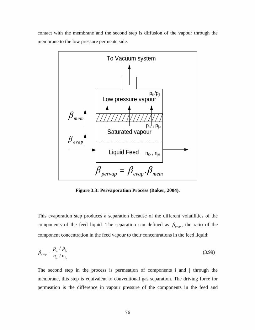
76
contact with the membrane and the second step is diffusion of the vapour through the
membrane to the low pressure permeate side.
mem
evap
pervap evap mem .
Liquid Feed
Saturated vapour
Low pressure vapour
To Vacuum system
nio , njo
pio , pjo
pil /pjl
Figure 3.3: Pervaporation Process (Baker, 2004).
This evaporation step produces a separation because of the different volatilities of the
components of the feed liquid. The separation can defined as evap , the ratio of the
component concentration in the feed vapour to their concentrations in the feed liquid:
evap
i j
i j
p p
n no o
o o
/
/ (3.99)
The second step in the process is permeation of components i and j through the
membrane, this step is equivalent to conventional gas separation. The driving force for
permeation is the difference in vapour pressure of the components in the feed and
77
permeates vapours (Baker, 2004). The separation factor defined as mem , is the ratio of the
components in the permeate vapour to the ratio of the components in the feed vapour:
mem
i j
i j
p p
p pl l
o o
/
/ (3.100)
Therefore, the separation factor achieved in pervaporation is equal to the product of the
separation achieved by evaporation of the liquid and the separation achieved by selective
permeation through the membrane:
pervap evap mem ( )( ) (3.101)
The evaporation separation factor, evap for the azeotropic mixture is 1 because, at the
azeotropic concentration of the vapour and liquid phases have the same composition and
is equal 1 again in the closely boiling point mixture, but a substantial separation is
achieved due to the greater permeability of the membrane for the aromatic components.
The membrane fluxes can be written as
JP p p
li
i
G
io i l( )
(3.102)
JP p p
lj
j
G
jo j l( )
(3.103)
Dividing equation 3.102 by equation 3.103
J
J
P p p
P p p
i
j
i
G
io i l
j
G
jo j l
( )
( ) (3.104)
The fluxes Ji and Jj in equation 3.102 and 3.103 are weight fluxes (g/cm2.s), similarly the
permabilities Pi
G and Pj
G are weight based (g.cm/cm
2.s.cmHg). The equation 3.97 is
more conveniently written in molar terms as
j
j
P p p
p p
i
j
i
G
io i l
j
G
jo j l
( )
( ) , (3.105)
78
In these case ji and jj are molar fluxes with unit (mol/cm2) or cm
3 (STP)/cm
2.s , Pi
G and
Pj
Gand molar permeabilities with units mol.cm/cm
2.s unit pressure or
cm3(STP).cm/cm
2.s.cmHg). The ratio of the molar membrane permeability coefficient
Pi
G / Pj
G is the conventional gas membrane selectivity,mem .
The ratio of the molar fluxes is also similar as the ratio of the permeate partial pressures
j
j
p
p
i
j
i l
j l
(3.106)
Combining Equations 3.99, 3.100, 3.105 and 3.106
pervap
evap mem io i l
jo j l io jo
p p
p p p p
( )
( )( / ) (3.107)
Equation 3.107 identifies the three factors that determine the performance of a
pervaporation system. The first factor, evap , is the vapour-liquid equilibrium, determined
mainly by the feed liquid composition and temperature. The second in the membrane
selectivity, mem , an intrinsic permeability property of the membrane material and the
third includes the feed and permeate vapour pressure, reflecting the effect of operating
parameters on membrane performance,mem .
According to Teng et al. (2000) the separation factor of ethanol/water is given by
Equation (3.108)
ethanolwater
ethanolwater
XX
YY
/
/ (3.108)
Where Yethanol and Ywater are represents the weight fractions of ethanol and water in the
permeate. Xethanol and Xwater are representing the weight fractions of ethanol and water in
the feed.
In this study, pervaporation membrane flux was calculated using the following equations
79
sm
kgdensity
areasurface
flowrateVolumetricJ
.*
2 (3.109)
Or TA
QJ
* (3.110)
Where Q is the total mass of permeate collected through the effective area of membrane
(A) during time, T is the temperature after the steady state has been reached.
80
CHAPTER 4
EXPERIMENTAL PROCEDURE
PART I: VAPOUR-LIQUID EQUILIBRUIM
4.1 Introduction
In this chapter, the experimental equipment and procedures are presented. The equipment
used for the assessment of salt as an extractive agent was a low pressure VLE still of
Joseph (2001) and associated chemicals analysis equipment. The equipment used for the
pervaporation studies was a unit constructed and tested specifically for this study. Details
of the constructed unit and the associated analysis equipment are presented.
The criteria used for choosing the test system were:
The system must be non-ideal (the classification of Danner and Gess, 1990) for
ideal and non-ideal system was used)
The literature data for the binary system must be consistent
The chemicals of the binary system must be available at a high purity (>99% pure)
The chemical must be available at a reasonable cost
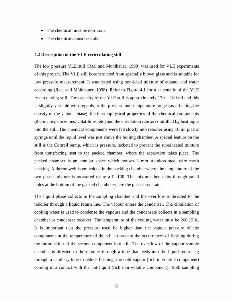
81
The chemical must be non-toxic
The chemicals must be stable
4.2 Description of the VLE recirculating still
The low pressure VLE still (Raal and Mühlbauer, 1998) was used for VLE experiments
of this project. The VLE still is constructed from specially blown glass and is suitable for
low pressure measurement. It was tested using non-ideal mixture of ethanol and water
according (Raal and Mühlbauer, 1998). Refer to Figure 4.1 for a schematic of the VLE
re-circulating still. The capacity of the VLE still is approximately 170 – 180 ml and this
is slightly variable with regards to the pressure and temperature range (as affecting the
density of the vapour phase), the thermophysical properties of the chemical components
(thermal expansivities, volatilities, etc) and the circulation rate as controlled by heat input
into the still. The chemical components were fed slowly into reboiler using 10 ml plastic
syringe until the liquid level was just above the boiling chamber. A special feature on the
still is the Cottrell pump, which is pressure, jacketed to prevent the superheated mixture
from transferring heat to the packed chamber, where the separation takes place. The
packed chamber is an annular space which houses 3 mm stainless steel wire mesh
packing. A thermowell is embedded in the packing chamber where the temperature of the
two phase mixture is measured using a Pt-100. The mixture then exits through small
holes at the bottom of the packed chamber where the phases separate.
The liquid phase collects in the sampling chamber and the overflow is directed to the
reboiler through a liquid return line. The vapour enters the condenser. The circulation of
cooling water is used to condense the vapours and the condensate collects in a sampling
chamber or condenser receiver. The temperature of the cooling water must be 268.15 K.
It is important that the pressure used be higher than the vapour pressure of the
components at the temperature of the still to prevent the occurrences of flashing during
the introduction of the second component into still. The overflow of the vapour sample
chamber is directed to the reboiler through a tube that feeds into the liquid return leg
through a capillary tube to reduce flashing, the cold vapour (rich in volatile component)
coming into contact with the hot liquid (rich non volatile component). Both sampling
82
chambers contain magnetic stirrers to reduce flashing and uniform composition. These
chambers allows for sampling through septa without interrupting the boiling.
Heating supplied in the boiling chamber
There are two heaters connected in the boiling chamber or reboiler. These are internal
and external heaters. The external heater of the equilibrium chamber was then turned on
and initial heating was at a low voltage input (usually 20V) from the respective Chuan
HSIN (model: SRV – 10) variable voltage transformers (0 – 240V). This compensates for
heat loss to the surroundings. The internal heater is used to directly control boiling or
smooth boiling of the mixture. Increasing the voltage the internal heater with the small
increment until the plateau region is reached. The mixture was heated in the boiling
chamber or the reboiler via a cartridge heater, which heats the inside of the chamber,
while a nichrome wire wrapped around the chamber heats the outer surface of the
chamber. The cartridge sits in a glass sheath which has the surface exposed to the liquid
activated with powered glass in order to promote vapour bubble formation.
The Limitations of LPVLE dynamic still
The greatest limitations in the operation of LPVLE dynamic recirculation apparatus are:
The attainment of a true equilibrium (Marsh, 1989).
The partial condensation of the vapour phase in the equilibrium chamber.
The inability to achieve smooth boiling and an equilibrium state with minimal
fluctuations in pressure and temperature.
Avoid superheating of the mixture.
The determination of the true values of equilibrium temperature and vapour
compositions (Abbott, 1986).
83
Experimental requirement
In order to obtain the isobaric VLE data, certain parameters need to be determined
experimentally or controlled:
Pressure in the still must be controlled and maintained steady
Equilibrium temperature of the vapour and liquid must be measured
The vapour and liquid sample must be taken at time intervals and must be
analyzed using a gas chromatograph for mole fractions of the respective
components
Chemicals
The non-ideal mixtures ethanol-water system was used in the VLE still. Distilled water,
high purity acetone (99.2%), high purity ethanol (99.5%) and calcium chloride salt were
used. Ethanol and acetone were purchased from Merck Chemicals Laboratories and
calcium chloride was purchased from DLD Scientific. The acetone was used for cleaning
purposes. The chilling water from Labcon low temperature water bath CPM 50 was used
as a coolant in the shell of the condenser at the temperature of 268.15 K.
Equipment
The precision class A Pt-100 temperature probe was used to measure equilibrium
temperature with a minimum error of ±0.01 K. The Pt-100 temperature probe was
calibrated using bath oil WIKA CTB 9100 and WIKA temperature probe which was
connected to WIKA CTH 6500 multi-meter. The uncertainty in the temperature reading
was ± 0.03 K. Measured equilibrium temperature was interpreted and display in ohms by
the Agilent digital multi-meter.
The pressure was controlled below atmospheric using a KNF vacuum pump controller
(type NC800). The system pressure was monitored with the aid of a Sensotec Super TJE
pressure transducer. The pressure was set using BÜCHI vacuum controller B-721 and the
signal from the transducer was interpreted and displayed in „kPa‟ by a Sensotec Model
84
HM display. The pressure display was calibrated with WIKA CPH 6000 unit. The
uncertainty in the pressure reading was ± 0.05 kPa.
The thermodynamic equilibrium was estimated to be reached when the pressure
measured remained constant for at least 45 minutes. Thereafter, vapour and liquid
samples were withdrawn for composition analysis. The analytical tool used was a gas
chromatograph Shimadzu, type HP 5890 series II. Each vapour and liquid was analysed
three times in the GC to determine vapour and liquid composition, with the average of the
three being taken as the final value. The separation was performed using a LANGET
column, 3 m length, 2.2 mm i.d., o.d 3.2 mm, column material S/S and support was
carbosieve S-11 using the helium as the carrier gas at a pressure of 150 kPa. The
maximum column temperature was 523.15 K. The analysis was realized using a thermal
conductivity detector (TCD) kept at column temperature of 453.15 K with a current set at
70 mA. The procedure for calibrating the GC was the area ratio method, as discussed by
Raal and Mühlbauer (1998).
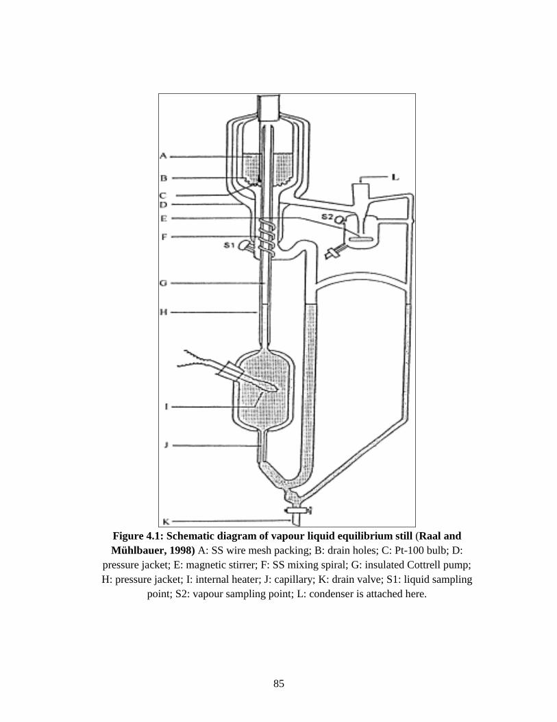
85
Figure 4.1: Schematic diagram of vapour liquid equilibrium still (Raal and
Mühlbauer, 1998) A: SS wire mesh packing; B: drain holes; C: Pt-100 bulb; D:
pressure jacket; E: magnetic stirrer; F: SS mixing spiral; G: insulated Cottrell pump;
H: pressure jacket; I: internal heater; J: capillary; K: drain valve; S1: liquid sampling
point; S2: vapour sampling point; L: condenser is attached here.
86
4.3 Experimental procedure for the VLE still
Air Leaks
An air leak test was performed by drawing a vacuum in the dry still, using a vacuum
pump at low pressure of 20 kPa. When pressure was reached 20 kPa, the pressure pump
was switch off. Air leak in the system can be identified by the increase in pressure or the
controller is not reached the set point. Then check all drain valves that are fully closed
and joins, fittings and septa in the VLE still. A very small air leak in the system causes
one of the components in the VLE still to evaporate.
Start-Up Procedure
Check that all the drain valves that are closed
Add approximately 80ml of component one through the liquid sampling septum
into the reboiler. Allow for the capillary tube to raise at least 3 – 4 cm above
reboiler.
Close both liquid and vapour sampling septum points
Switch on Pt-100 temperature sensor
Set pressure at 40 kPa and switch on pressure pump
Set chilling water temperature at 268.15 K and allow chilling water to circulate in
the condenser
Wait for chilling water temperature and the pressure to reached the set points
Switch on internal and external heaters
Set external heater at 40 Volts
Switch on both magnetic stirrers
Find the plateau* region by increasing the voltage of the internal heater with a
small increment (5 Volts).
Record temperature and pressure
Switch off internal and external heaters
Add component two in 3ml increments into the liquid sampling port; switch on
internal and external heaters and find the plateau region for each mixture
composition
87
Take 1µL liquid and vapour samples, at regular intervals, through their respective
sampling septa for analysis in the GC
Normally the equilibrium is attained in 60 minutes.
Shut down Procedure
Turn off heaters, magnetic stirrer and vacuum pump
Set atmospheric pressure by opening both liquid and vapour sampling septum
(slowly)
Stop cooling water circulation in the condenser
Open drain valve to empty the VLE still
Cleaning the VLE Still
This is done by circulating acetone in the VLE still under atmospheric pressure
Add 80ml of acetone into the still via the liquid sampling septum
Set atmospheric pressure
Find plateau*region. Allow the acetone to boil for 45 minutes and collect liquid
and vapour samples for GC analysis. If the samples showing more than one peak
on a gas chromatograph then repeat acetone wash until the gas chromatograph
reveals one acetone peak.
Drain out acetone by opening drain valves.
Set the pressure at 20 kPa and switch on the vacuum pump for 10 minutes to dry
the acetone residue from still.
4.4 VLE Still Setup
The condenser of the VLE still is connected to the ballast flask, which serves to reduce
pressure fluctuations and to trap condensable chemicals if the condenser fails. A vacuum
pump controller unit was used to evacuate the still and to maintain a constant pressure.
The vacuum pump draws incondensable gases from the VLE still. Once the set point
pressure has been achieved the controller shuts off the vacuum pump. If and when this set
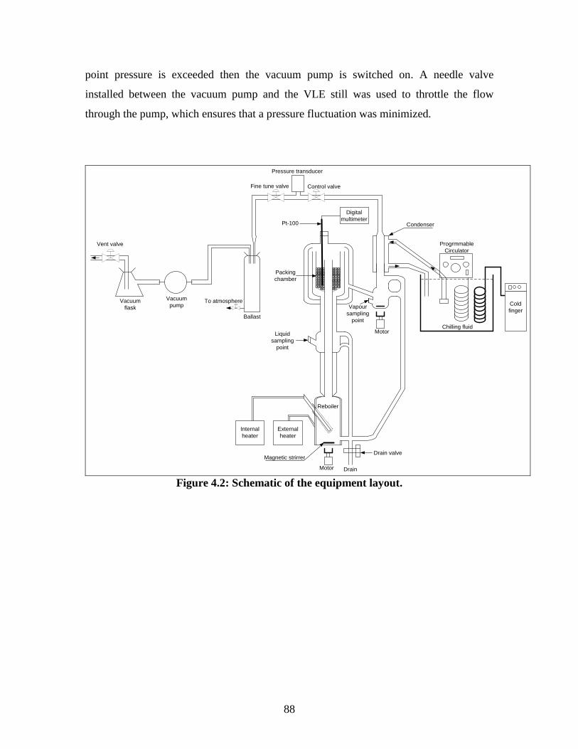
88
point pressure is exceeded then the vacuum pump is switched on. A needle valve
installed between the vacuum pump and the VLE still was used to throttle the flow
through the pump, which ensures that a pressure fluctuation was minimized.
Chilling fluid
Cold
finger
Progrmmable
Circulator
External
heater
Internal
heater
Control valveFine tune valve
Vent valve
Vacuum
pumpVacuum
flask
Ballast
To atmosphere
Pressure transducer
Digital
multimeterCondenserPt-100
Packing
chamber
Magnetic strirrer
Motor Drain
Drain valve
Reboiler
Motor
Vapour
sampling
point
Liquid
sampling
point
Figure 4.2: Schematic of the equipment layout.
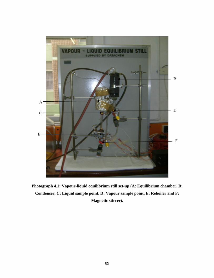
89
Photograph 4.1: Vapour-liquid equilibrium still set-up (A: Equilibrium chamber, B:
Condenser, C: Liquid sample point, D: Vapour sample point, E: Reboiler and F:
Magnetic stirrer).
B
A
A
C
E
F
D
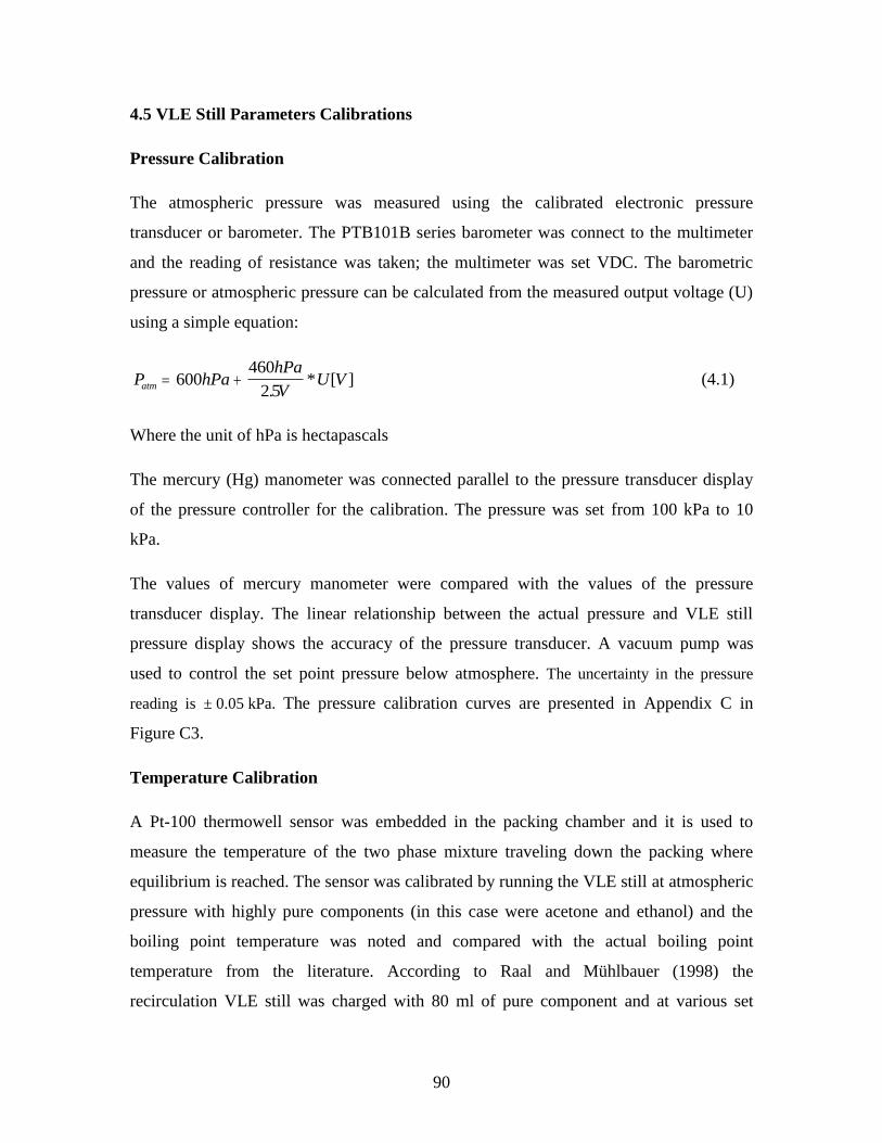
90
4.5 VLE Still Parameters Calibrations
Pressure Calibration
The atmospheric pressure was measured using the calibrated electronic pressure
transducer or barometer. The PTB101B series barometer was connect to the multimeter
and the reading of resistance was taken; the multimeter was set VDC. The barometric
pressure or atmospheric pressure can be calculated from the measured output voltage (U)
using a simple equation:
P hPahPa
VU Vatm 600
460
25.* [ ] (4.1)
Where the unit of hPa is hectapascals
The mercury (Hg) manometer was connected parallel to the pressure transducer display
of the pressure controller for the calibration. The pressure was set from 100 kPa to 10
kPa.
The values of mercury manometer were compared with the values of the pressure
transducer display. The linear relationship between the actual pressure and VLE still
pressure display shows the accuracy of the pressure transducer. A vacuum pump was
used to control the set point pressure below atmosphere. The uncertainty in the pressure
reading is ± 0.05 kPa. The pressure calibration curves are presented in Appendix C in
Figure C3.
Temperature Calibration
A Pt-100 thermowell sensor was embedded in the packing chamber and it is used to
measure the temperature of the two phase mixture traveling down the packing where
equilibrium is reached. The sensor was calibrated by running the VLE still at atmospheric
pressure with highly pure components (in this case were acetone and ethanol) and the
boiling point temperature was noted and compared with the actual boiling point
temperature from the literature. According to Raal and Mühlbauer (1998) the
recirculation VLE still was charged with 80 ml of pure component and at various set
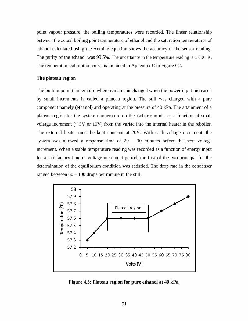
91
point vapour pressure, the boiling temperatures were recorded. The linear relationship
between the actual boiling point temperature of ethanol and the saturation temperatures of
ethanol calculated using the Antoine equation shows the accuracy of the sensor reading.
The purity of the ethanol was 99.5%. The uncertainty in the temperature reading is ± 0.01 K.
The temperature calibration curve is included in Appendix C in Figure C2.
The plateau region
The boiling point temperature where remains unchanged when the power input increased
by small increments is called a plateau region. The still was charged with a pure
component namely (ethanol) and operating at the pressure of 40 kPa. The attainment of a
plateau region for the system temperature on the isobaric mode, as a function of small
voltage increment (~ 5V or 10V) from the variac into the internal heater in the reboiler.
The external heater must be kept constant at 20V. With each voltage increment, the
system was allowed a response time of 20 – 30 minutes before the next voltage
increment. When a stable temperature reading was recorded as a function of energy input
for a satisfactory time or voltage increment period, the first of the two principal for the
determination of the equilibrium condition was satisfied. The drop rate in the condenser
ranged between 60 – 100 drops per minute in the still.
Figure 4.3: Plateau region for pure ethanol at 40 kPa.
Plateau region

92
Gas chromatography (GC) Calibration
It is important to calibrate the GC detector (Raal and Mühlbauer, 1998) as the percentage
composition given by the integrator may not be a true representation of component mole
fraction. Binary systems exhibit the following relationship in the dilute regions.
x
x G
A
A
n
n
1
2
1
2
1
2
1 (4.2)
where: x = mole fraction in the sample
A = is the produced by the GC integrator or GC peak area
G = is the response factor
The determination of vapour and liquid sample composition of the binary mixture are
gravimetrically produced and analysed by the GC. As ternary measurements were all on a
solvent-free basis binary calibrations were sufficient. The prepared samples covered the
composition range of mole ratios equal to 0 up to 1.2.. Six or more samples are usually
necessary for calibration. Two plots are produced from the calibration data. The first is a
plot of x1/x2 vs A1/A2 and the x1/x2 values range from 0 to 1.5. The second plot is x2/x1 vs
A2/A1 with the range values of 0 to 1.2. Both plots are linear and the gradient of plot 1 is
compared to the inverse of the gradient of plot 2. The gradient is equated to the response
factor (Raal and Mühlbauer, 1998). The uncertainty in the GC detector for the composition
analysis for the systems investigated is ± 0.005.
To solve for the individual mole fractions or compositiona, using the GC Areas obtained
from the chromatograph, if x2/x1 = a and for ternary measurements x3/x1 = b, x4/x1 = c,
etc, then:
for a binary system
11 1
1
2
1x
x
xa (4.3)
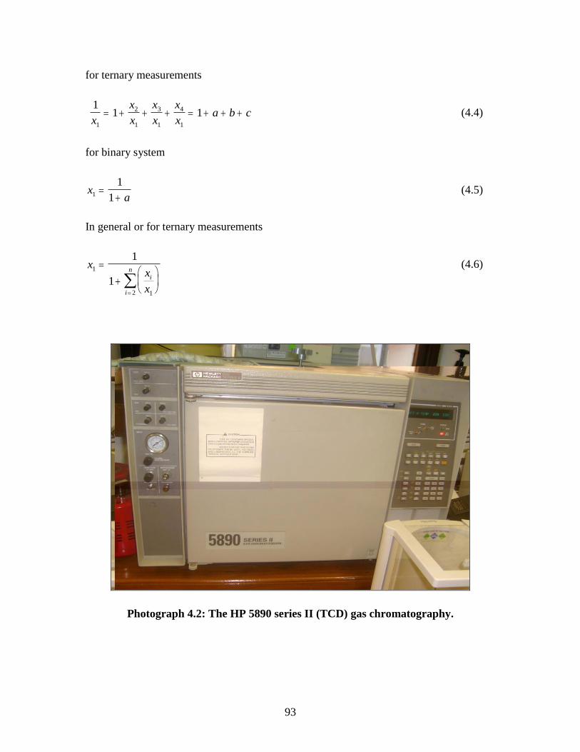
93
for ternary measurements
1
1 11
2
1
3
1
4
1x
x
x
x
x
x
xa b c (4.4)
for binary system
xa1
1
1
(4.5)
In general or for ternary measurements
xx
x
i
i
n1
12
1
1
(4.6)
Photograph 4.2: The HP 5890 series II (TCD) gas chromatography.
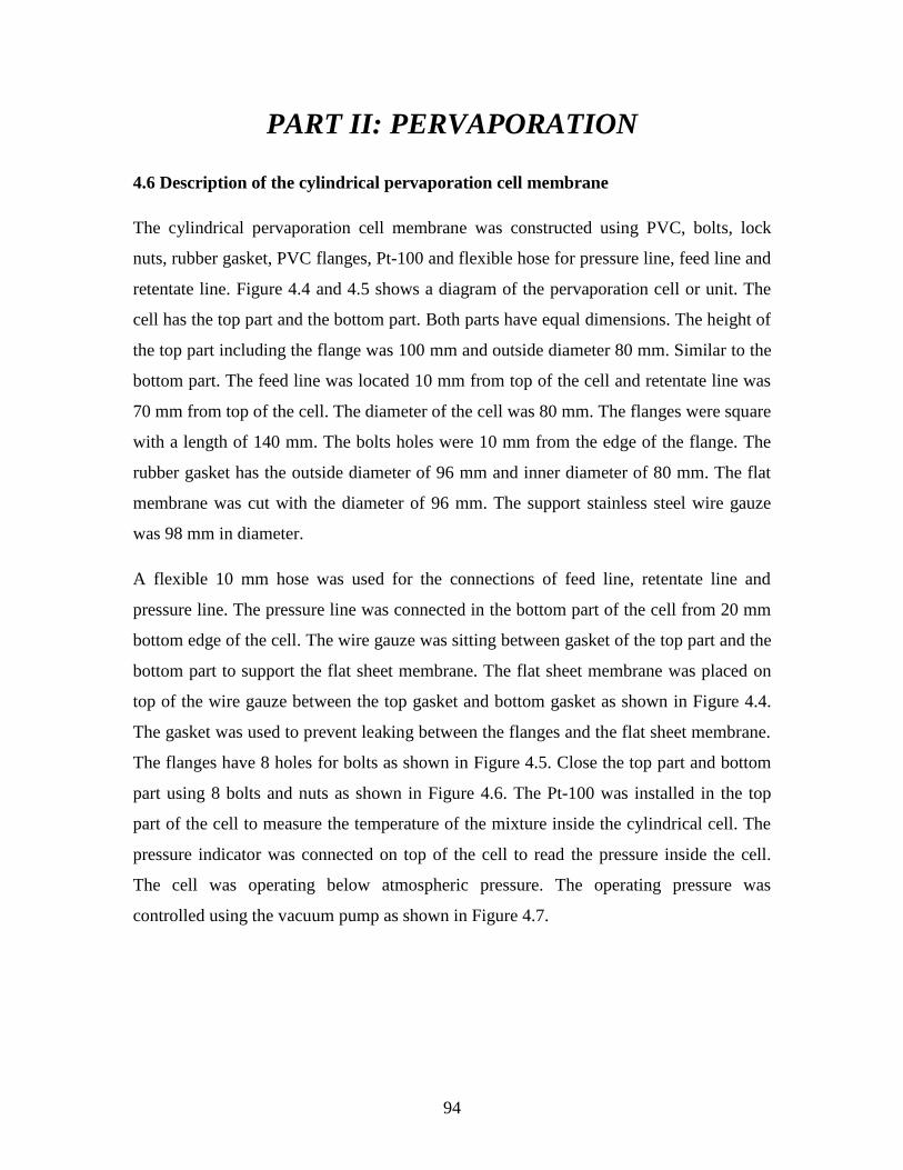
94
PART II: PERVAPORATION
4.6 Description of the cylindrical pervaporation cell membrane
The cylindrical pervaporation cell membrane was constructed using PVC, bolts, lock
nuts, rubber gasket, PVC flanges, Pt-100 and flexible hose for pressure line, feed line and
retentate line. Figure 4.4 and 4.5 shows a diagram of the pervaporation cell or unit. The
cell has the top part and the bottom part. Both parts have equal dimensions. The height of
the top part including the flange was 100 mm and outside diameter 80 mm. Similar to the
bottom part. The feed line was located 10 mm from top of the cell and retentate line was
70 mm from top of the cell. The diameter of the cell was 80 mm. The flanges were square
with a length of 140 mm. The bolts holes were 10 mm from the edge of the flange. The
rubber gasket has the outside diameter of 96 mm and inner diameter of 80 mm. The flat
membrane was cut with the diameter of 96 mm. The support stainless steel wire gauze
was 98 mm in diameter.
A flexible 10 mm hose was used for the connections of feed line, retentate line and
pressure line. The pressure line was connected in the bottom part of the cell from 20 mm
bottom edge of the cell. The wire gauze was sitting between gasket of the top part and the
bottom part to support the flat sheet membrane. The flat sheet membrane was placed on
top of the wire gauze between the top gasket and bottom gasket as shown in Figure 4.4.
The gasket was used to prevent leaking between the flanges and the flat sheet membrane.
The flanges have 8 holes for bolts as shown in Figure 4.5. Close the top part and bottom
part using 8 bolts and nuts as shown in Figure 4.6. The Pt-100 was installed in the top
part of the cell to measure the temperature of the mixture inside the cylindrical cell. The
pressure indicator was connected on top of the cell to read the pressure inside the cell.
The cell was operating below atmospheric pressure. The operating pressure was
controlled using the vacuum pump as shown in Figure 4.7.
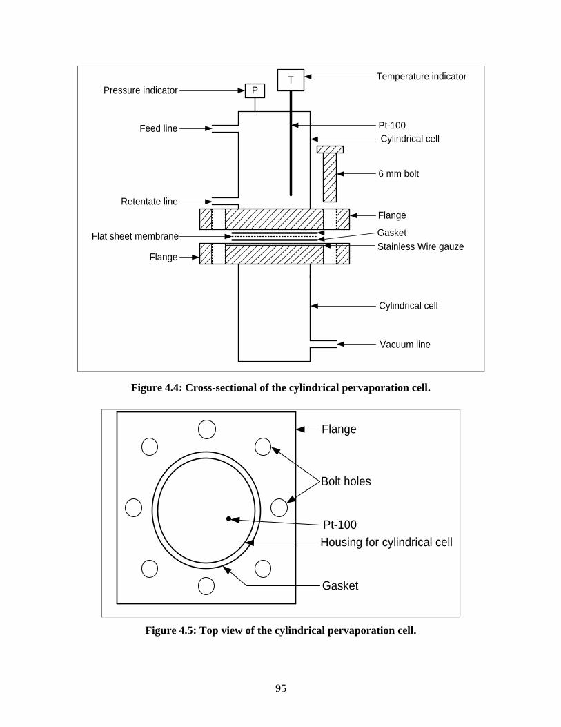
95
Pt-100
Vacuum line
6 mm bolt
Flat sheet membrane
Feed line
Pressure indicator
Retentate line
Flange
Temperature indicator
Cylindrical cell
Gasket
Flange
Cylindrical cell
TP
Stainless Wire gauze
Figure 4.4: Cross-sectional of the cylindrical pervaporation cell.
Gasket
Bolt holes
Housing for cylindrical cell
Pt-100
Flange
Figure 4.5: Top view of the cylindrical pervaporation cell.

96
Check air leak
In order to check for air leaks, the cylindrical cell was closed tightly and connected to a
vacuum pump. The feed and retentate valves were closed. The vacuum pump was
switched on and set at a low pressure of 20 kPa. Once a pressure of 20 kPa was reached,
Snoop® was used to check for leaks in the pipe connections, flanges and lock nuts.
Before switching on the system, the pressure was set at 20 kPa and one had to wait for 15
minutes. If the set pressure was not reached or there were fluctuates, then there was a
possibility of leaks somewhere in the system. The air leaks could cause the ethanol to
evaporate or water vapour to escape.
Description of the pervaporation process
The heated mixture of ethanol and water in the storage feed tank was pumped using an
adjustable centrifugal pump to the filter. The mixture from the filter was passed through
the flow meter and entered at the top of the cylindrical membrane cell. The pump was run
at the different speeds to change the flow rates. The separation of the ethanol/water
mixture took place inside the cylindrical membrane cell. The vacuum pump was
connected to the top of the condenser using vacuum tubing. The vacuum in the cell was
drawn through the vacuum line attached to the bottom part of the cell via the condenser.
The condenser was connected at the top of the permeate tank. The chilling water was
circulated in the shell of the condenser at the temperature of 268.15 K. As the vacuum
pump drew the water vapour from the membrane from the cell, the water vapour
condensed. The liquid was collected in the permeate tank. The vacuum flask was used to
collect excess gas and it was connected in line with the vacuum pump as shown in Figure
4.7. The samples were taken from the collected volume in the permeate tank and in the
feed tank for analysis. The refractometer and Karl-Firscher apparatus were used for
analyses.
Ethanol of 99.5% purity was diluted with distill water to the concentration of 90 wt%
ethanol and 10 wt% water. The acetone was used for cleaning. The separation of ethanol-
water system at concentrations of 90% ethanol and 10% water to 99% ethanol to 1%
water was studied using pervaporation at different operating pressure from 20 kPa to 80
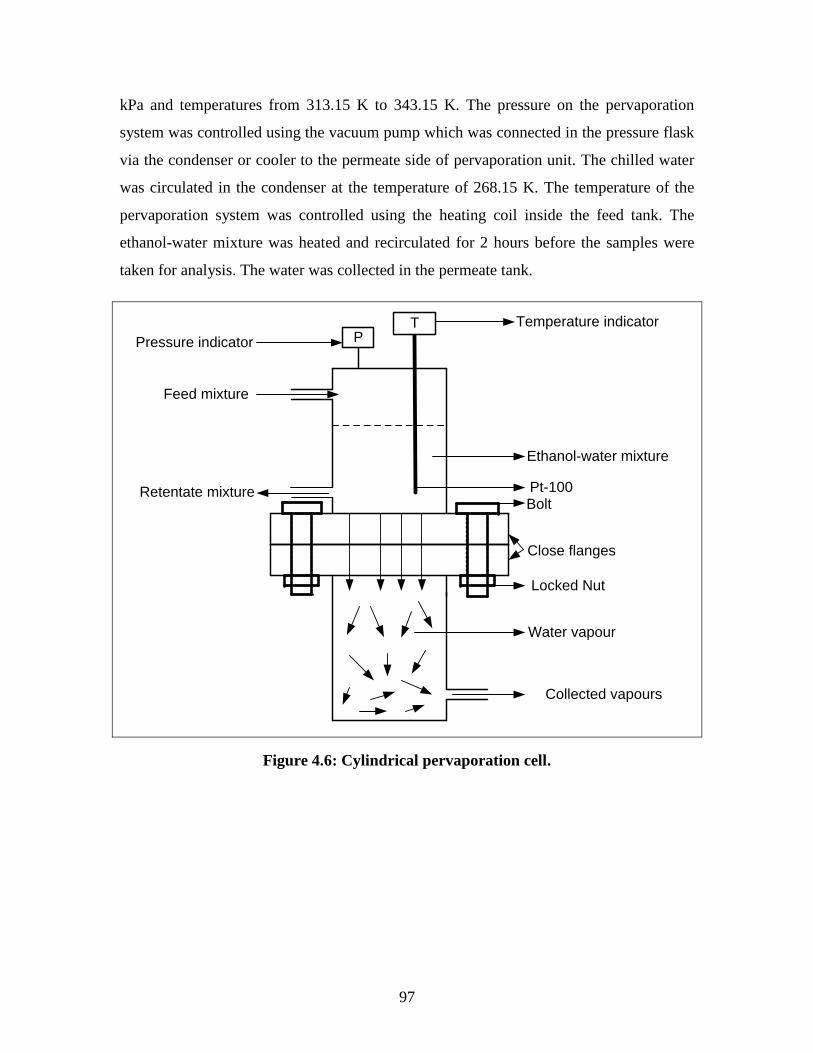
97
kPa and temperatures from 313.15 K to 343.15 K. The pressure on the pervaporation
system was controlled using the vacuum pump which was connected in the pressure flask
via the condenser or cooler to the permeate side of pervaporation unit. The chilled water
was circulated in the condenser at the temperature of 268.15 K. The temperature of the
pervaporation system was controlled using the heating coil inside the feed tank. The
ethanol-water mixture was heated and recirculated for 2 hours before the samples were
taken for analysis. The water was collected in the permeate tank.
Temperature indicator
Pressure indicator
Feed mixture
Ethanol-water mixture
BoltPt-100
Locked Nut
Water vapour
Collected vapours
Close flanges
Retentate mixture
TP
Figure 4.6: Cylindrical pervaporation cell.
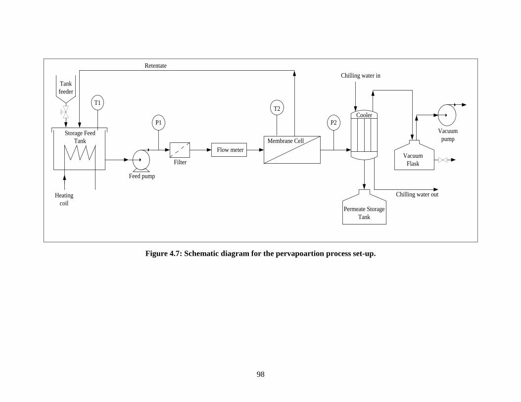
98
Membrane Cell
Retentate
Flow meter
P2
Chilling water in
Vacuum
Flask
Vacuum
pump
Permeate Storage
Tank
T2
Chilling water out
Cooler
Feed pump
Filter
Storage Feed
Tank
Heating
coil
T1
P1
Tank
feeder
Figure 4.7: Schematic diagram for the pervapoartion process set-up.
99
Chemicals and materials
Distilled water, high purity acetone (99.2%) and high purity ethanol (99.5%) were used.
Ethanol and acetone were purchased from Merck Chemical Laboratories. The low
pressure pervaporation membrane cell was design and constructed at the School of
Chemical Engineering, Durban University of Technology. The pervaporation polymer
dehydration membrane was purchased from Sulzer Chemtech in Germany and this
membrane was a composite membrane consisting of a very thin separation layer on top of
a porous support, coated on a polymer fleece. The type of the pervaporation membrane
used in this study was composite flat sheet membrane 1210 and the specification is listed
in Table 4.2. The active area of the pervaporation membrane used in the cell was 0.0055
m2 and the membrane was supported by wire gauze. In this study, the pervaporation
membrane used was a hydrophilic membrane; which is a membrane that removes water.
The chilling water from the Labcon low temperature water bath CPM 50 was used as a
coolant in the shell of the condenser at the temperature of 268.15K.
Equipment
A precision class A Pt-100 temperature probe was used to measure the temperature inside
the pervaporation cell with a minimum error of 0.01K. The Pt-100 temperature probe was
calibrated using bath oil WIKA CTB 9100 and WIKA temperature probe which was
connected to WIKA CTH 6500 multi-meter. The measured equilibrium temperature was
interpreted and display by a Sensotec Model HM display.
The pressure was controlled below atmospheric using a KNF vacuum pump controller
(Model NSE 800). The system pressure was monitored with the aid of a WIKA pressure
transducer (Model D – 10 – P) and it range from 0 – 1.6 bar absolute. The pressure was
set using BÜCHI vacuum controller V–800 and the signal from the transducer was
interpreted and displayed in „kPa‟ by a Sensotec Model HM display. The pressure
transducer was calibrated using WIKA instrument CPH 6000 unit. A Watson Marlow
(peristaltic pump 323 or centrifugal pump) was used to pump the ethanol/water mixture
from the storage feed tank to the pervaporation cell. Polyscience circulator temperature
controller was used to heat the water in the water bath in order to heat the mixture to the
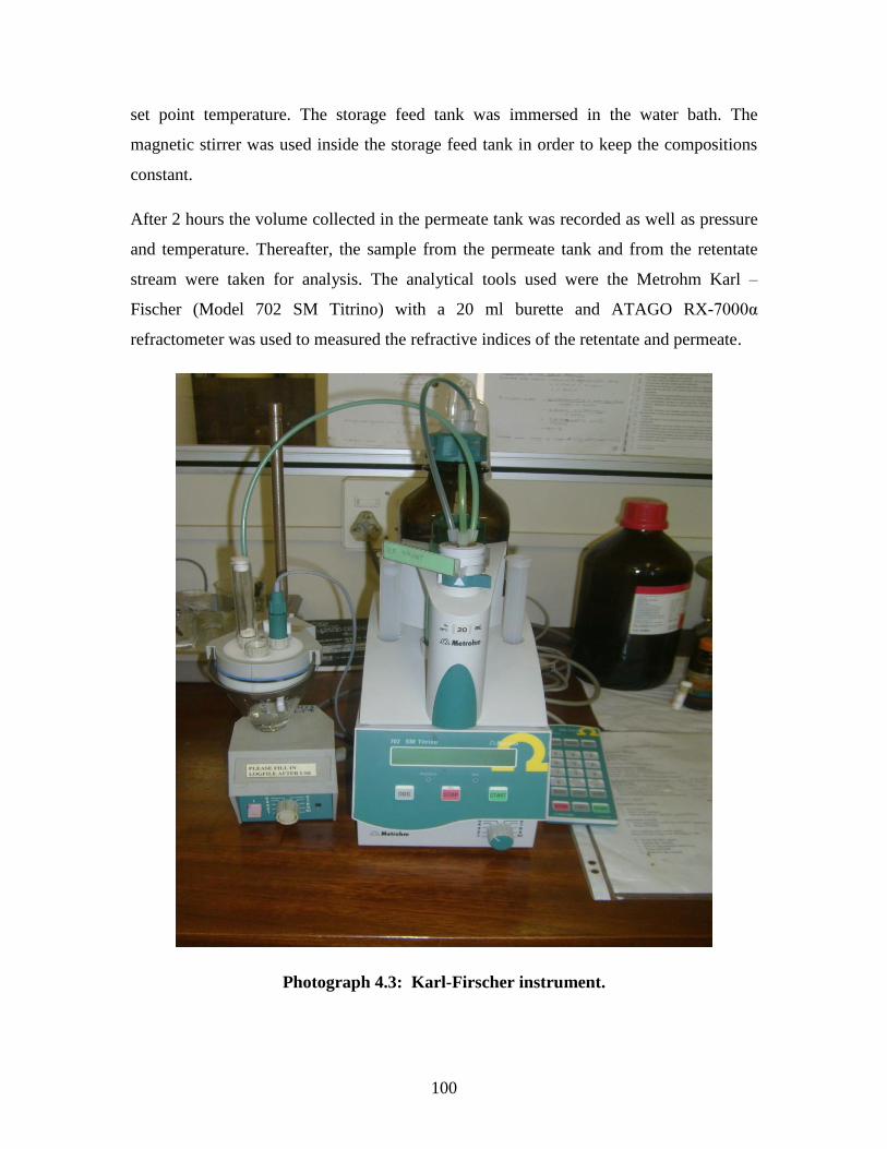
100
set point temperature. The storage feed tank was immersed in the water bath. The
magnetic stirrer was used inside the storage feed tank in order to keep the compositions
constant.
After 2 hours the volume collected in the permeate tank was recorded as well as pressure
and temperature. Thereafter, the sample from the permeate tank and from the retentate
stream were taken for analysis. The analytical tools used were the Metrohm Karl –
Fischer (Model 702 SM Titrino) with a 20 ml burette and ATAGO RX-7000α
refractometer was used to measured the refractive indices of the retentate and permeate.
Photograph 4.3: Karl-Firscher instrument.
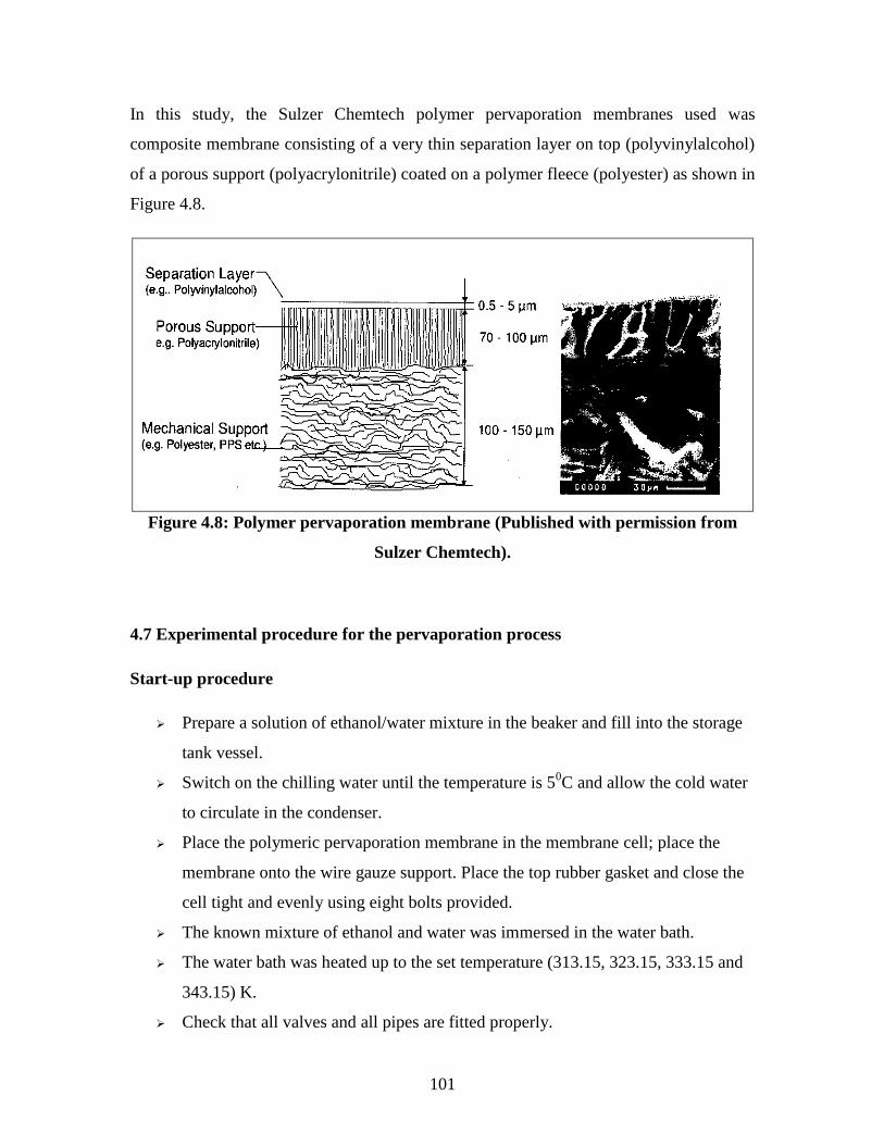
101
In this study, the Sulzer Chemtech polymer pervaporation membranes used was
composite membrane consisting of a very thin separation layer on top (polyvinylalcohol)
of a porous support (polyacrylonitrile) coated on a polymer fleece (polyester) as shown in
Figure 4.8.
Figure 4.8: Polymer pervaporation membrane (Published with permission from
Sulzer Chemtech).
4.7 Experimental procedure for the pervaporation process
Start-up procedure
Prepare a solution of ethanol/water mixture in the beaker and fill into the storage
tank vessel.
Switch on the chilling water until the temperature is 50C and allow the cold water
to circulate in the condenser.
Place the polymeric pervaporation membrane in the membrane cell; place the
membrane onto the wire gauze support. Place the top rubber gasket and close the
cell tight and evenly using eight bolts provided.
The known mixture of ethanol and water was immersed in the water bath.
The water bath was heated up to the set temperature (313.15, 323.15, 333.15 and
343.15) K.
Check that all valves and all pipes are fitted properly.
102
Set the operating pressure and start the pressure pump..
Wait for the system to stabilize.
Circulate the mixture in the feed tank until set temperature is reached.
Switch on the feed pump, then the mixture enters the pervaporation membrane
cell unit and re-circulate back into the feed tank.
Start the stop watch.
Wait for 2 hours to collect the volume of permeate (water).
Take a sample from the permeate tank and the retentate line for analysis
The sample must be taken every 2 hours.
Experimental run
This consisted of letting the run continue with sampling of the retentate and permeate
taken every two hours to verify that the composition was reproducible. When this was
satisfied then the composition of the feed was changed accordingly (after the refractive
index and hence the composition was known).
Shutdown procedure
Stop the pressure pump
Stop the feed pump
Switch off heaters in water bath
Wait for 5 minutes in order to collect all the condensed vapours
Open membrane cell unit
Remove the pervaporation membrane from the cell unit
Place the membrane on the clean flat surface.
Drain the feed tank
.
Cleaning procedure
Clean top and bottom the cylindrical cell with soft brush using acetone.
Clean the gasket, wire gauze support and bolts.

103
Close the cell and dry it under vacuum.
Open the cell to check that there is no black stain or black spot in the
pervaporation cell.
Rinse the feed tank with acetone and dry it.
Pervaporation test cell or calibration
The pervaporation method was tested at the high temperature and low pressure in order to
make sure that the pervaporation unit provides consistent results. The ethanol-water
mixture was prepared and run at the temperature of 343.15 K and pressure of 80 kPa. The
mixture was run at constant temperature and pressure for 10 hours, during the first 1-2
hours the water flux was increasing and from two hours to ten hours the water flux
obtained was constant and it showed that the volume collect every two hours was
constant. The volume collected during this period showed that the pervaporation cell
provides accurate results. This calibration was repeated twice for consistency. Figure 4.9
confirms that cell can be used to perform the ethanol-water system.
Figure 4.9: The pervaporation test of ethanol/water system at temperature of 343.15
K and pressure of 80 kPa.
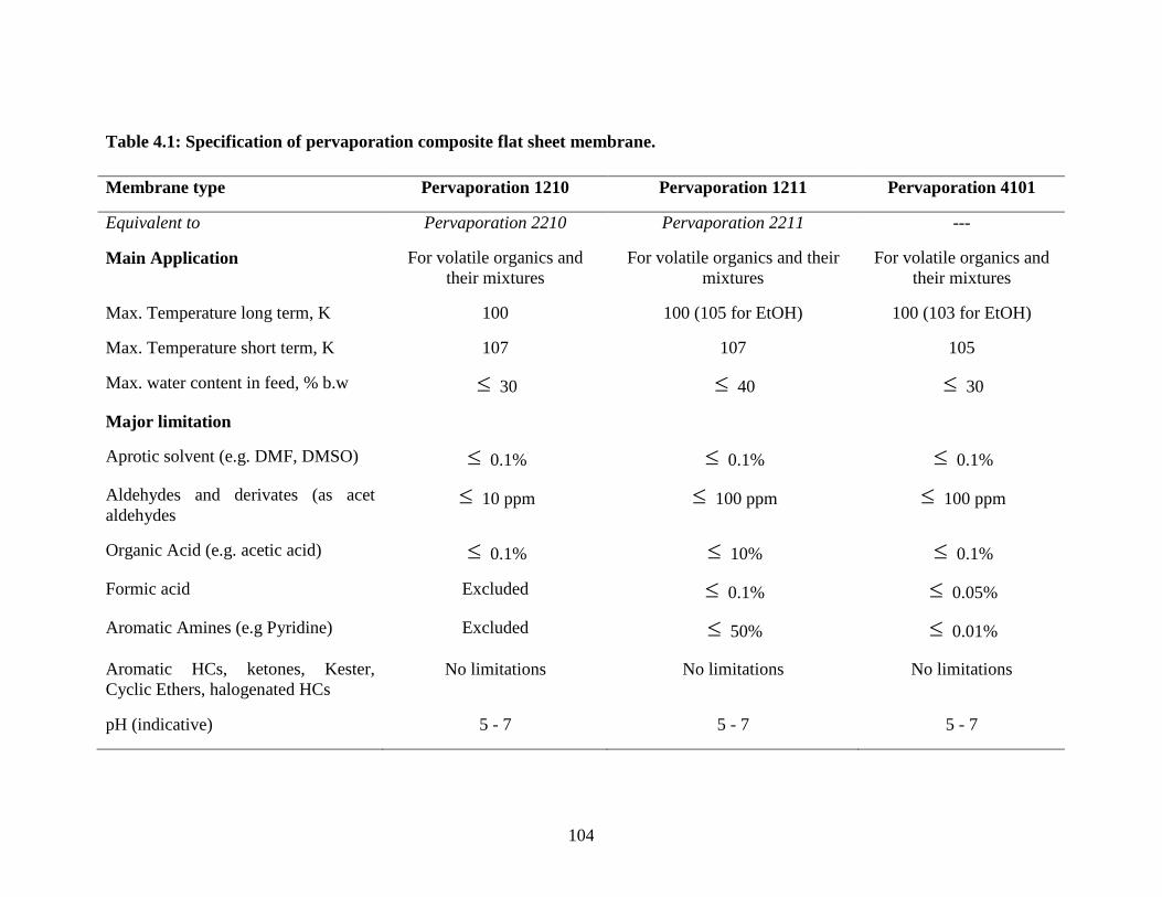
104
Table 4.1: Specification of pervaporation composite flat sheet membrane.
Membrane type Pervaporation 1210 Pervaporation 1211 Pervaporation 4101
Equivalent to Pervaporation 2210 Pervaporation 2211 ---
Main Application For volatile organics and
their mixtures
For volatile organics and their
mixtures
For volatile organics and
their mixtures
Max. Temperature long term, K 100 100 (105 for EtOH) 100 (103 for EtOH)
Max. Temperature short term, K 107 107 105
Max. water content in feed, % b.w 30 40 30
Major limitation
Aprotic solvent (e.g. DMF, DMSO) 0.1% 0.1% 0.1%
Aldehydes and derivates (as acet
aldehydes 10 ppm 100 ppm 100 ppm
Organic Acid (e.g. acetic acid) 0.1% 10% 0.1%
Formic acid Excluded 0.1% 0.05%
Aromatic Amines (e.g Pyridine) Excluded 50% 0.01%
Aromatic HCs, ketones, Kester,
Cyclic Ethers, halogenated HCs
No limitations No limitations No limitations
pH (indicative) 5 - 7 5 - 7 5 - 7
110
CHAPTER 5
RESULTS AND DISCUSSIONS
5.1 Introduction
The experimental and computational results for the salt assessment study and
pervaporation investigation are presented in this chapter. The ethanol-water system at 100
kPa was used as a test system and the baseline to see the effect of salt in the system at
different pressures and salt concentrations. The relative volatility has the value of unity at
the azeotropic point, and hence an increase in relative volatility value from unity will
mean an elimination of the azeotrope in the ethanol-water system. The experimental
vapour pressure data for ethanol and water were measured. The Wilson and NRTL
models were used for the data reduction of the salt experimental VLE data. Salt was not
used in the pervaporation because pervaporation has the advantage of direct separation.
The objectives of this study was met and are discussed in this Chapter (i) the effect of
operating pressure and operating temperature on the pervaporation process in order to
produce high purity ethanol and (ii) the effect of separating agent (calcium chloride salt)

111
and operating pressure in extractive distillation (VLE still) in order to produce high purity
ethanol.
5.2 Pure component properties
Ethanol and water purity were checked before use for this study to ensure that they were
not contaminated. The refractive index and conductivity of pure ethanol and distilled
water were measured and compared with the literature as shown in Table 5.1. The
deviation between literature and experimental values within uncetainties, and hence the
chemicals were not contaminated. Table 5.2 shows the physical properties of ethanol,
water and calcium chloride salt. The critical properties of ethanol and water play an
important role in the data reduction and data analysis.
Table 5.1: Refractive Index nD and conductivity.
Component Refractive Index at 293.15 K Conductivity
nD µS
Experimental Literaturea Experimental Literature
b
Ethanol 1.3605 1.3612 1.41 1.5
Water 1.334 1.336 4.98 2 - 5
a and b were literature values (Weast, 1983-1984)
Table 5.2: Physical properties of ethanol and water.
Component Boiling
point
Molecular
weight
Density Liquid
molar
volume
Purity
K g/mol kg/m3 cm
3/g.mol wt%
Ethanol 351.15 46 760.02 58.68 99.5
Water 373.15 18.02 1000.00 18.07 98.5
CaCl2 1873.15 110.98 2150.12 - 98
All these data were taken from Weast (1983-1984)
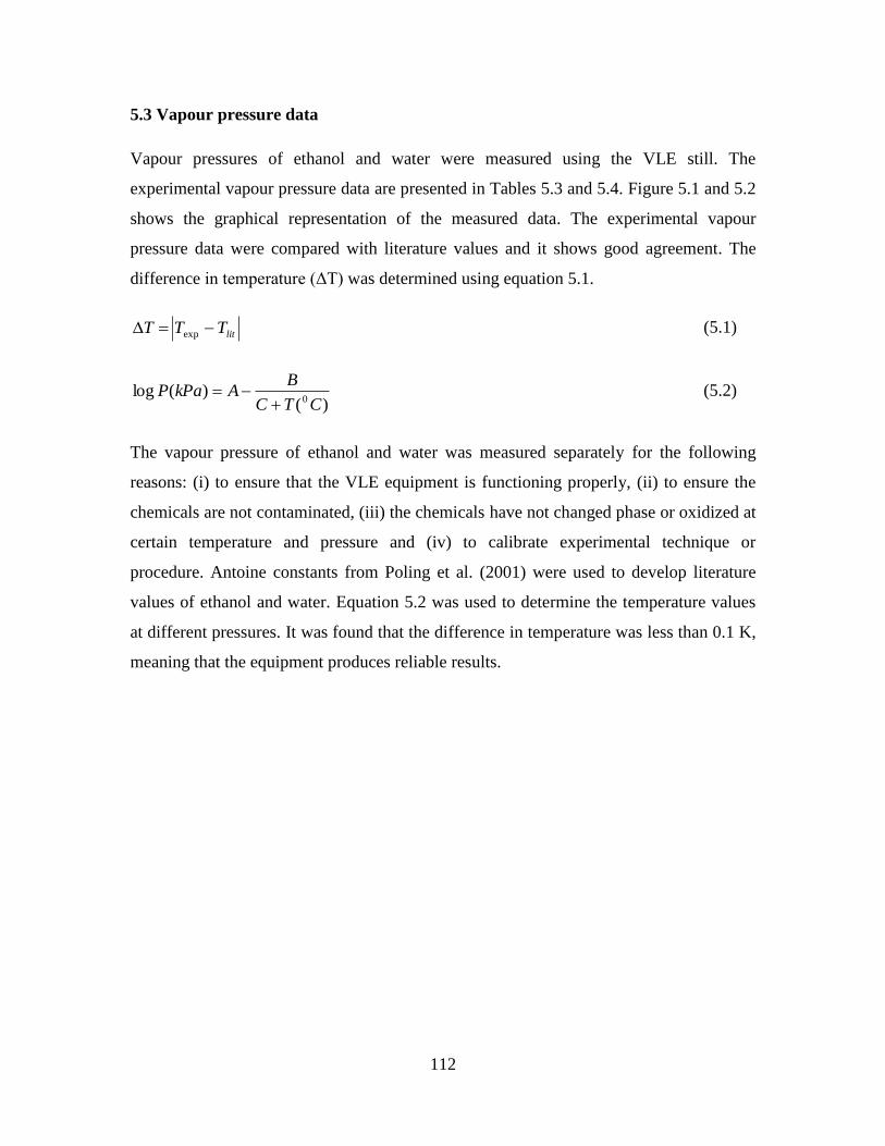
112
5.3 Vapour pressure data
Vapour pressures of ethanol and water were measured using the VLE still. The
experimental vapour pressure data are presented in Tables 5.3 and 5.4. Figure 5.1 and 5.2
shows the graphical representation of the measured data. The experimental vapour
pressure data were compared with literature values and it shows good agreement. The
difference in temperature (ΔT) was determined using equation 5.1.
litTTT exp (5.1)
)()(log
0 CTC
BAkPaP
(5.2)
The vapour pressure of ethanol and water was measured separately for the following
reasons: (i) to ensure that the VLE equipment is functioning properly, (ii) to ensure the
chemicals are not contaminated, (iii) the chemicals have not changed phase or oxidized at
certain temperature and pressure and (iv) to calibrate experimental technique or
procedure. Antoine constants from Poling et al. (2001) were used to develop literature
values of ethanol and water. Equation 5.2 was used to determine the temperature values
at different pressures. It was found that the difference in temperature was less than 0.1 K,
meaning that the equipment produces reliable results.
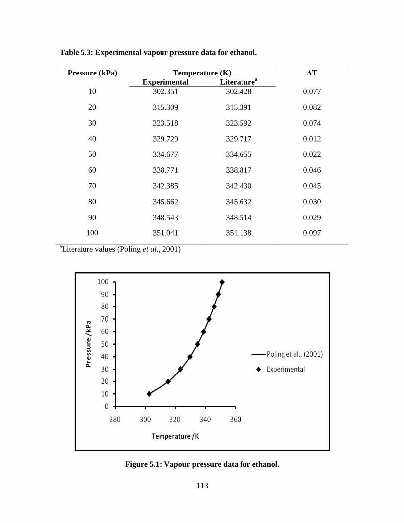
113
Table 5.3: Experimental vapour pressure data for ethanol.
Pressure (kPa) Temperature (K) ΔT
Experimental Literaturea
10 302.351 302.428 0.077
20 315.309 315.391 0.082
30 323.518 323.592 0.074
40 329.729 329.717 0.012
50 334.677 334.655 0.022
60 338.771 338.817 0.046
70 342.385 342.430 0.045
80 345.662 345.632 0.030
90 348.543 348.514 0.029
100 351.041 351.138 0.097
aLiterature values (Poling et al., 2001)
Figure 5.1: Vapour pressure data for ethanol.
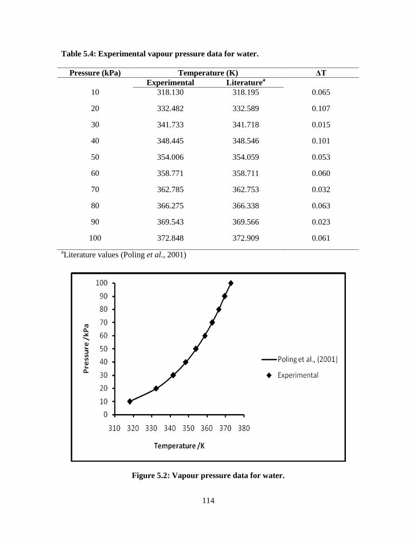
114
Table 5.4: Experimental vapour pressure data for water.
Pressure (kPa) Temperature (K) ΔT
Experimental Literaturea
10 318.130 318.195 0.065
20 332.482 332.589 0.107
30 341.733 341.718 0.015
40 348.445 348.546 0.101
50 354.006 354.059 0.053
60 358.771 358.711 0.060
70 362.785 362.753 0.032
80 366.275 366.338 0.063
90 369.543 369.566 0.023
100 372.848 372.909 0.061
aLiterature values (Poling et al., 2001)
Figure 5.2: Vapour pressure data for water.
115
5.4 Results of calibration of VLE still
Experimental VLE data for the ethanol-water system in the absence of salt at 100 kPa
was used to verify and test experimental technique and procedure of the dynamic VLE
still. The objectives for studying the VLE for this system in the absence of salt were: (i)
to check the practical feasibility of using the VLE still, (ii) to study the effect of having
active packing material on the VLE of binary mixtures, and (iii) to establish the baseline
for the ethanol-water system in order to see the effect of calcium chloride salt in the
system. This was done by comparing the results obtained using this still with published
results for the given system under same the conditions. Comparison of the measured
results was done with those published in literature (Ohe, 1991; Perry and Green, 1997). If
the data correspond with the literature values, a high degree of confidence can be placed
in the correct functioning of the equipment. Table 5.5 shows the experimental VLE data
for ethanol and water system without salt addition. Figure 5.3 indicates the ethanol-water
system without salt and Figure 5.4 represents the temperature vapour-liquid diagram.
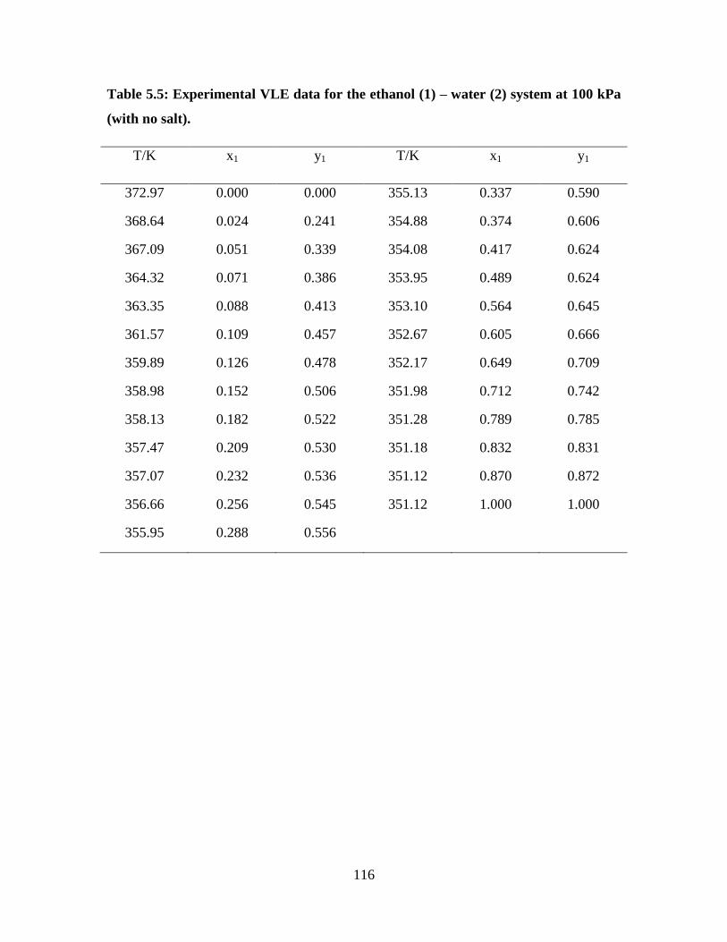
116
Table 5.5: Experimental VLE data for the ethanol (1) – water (2) system at 100 kPa
(with no salt).
T/K x1 y1 T/K x1 y1
372.97 0.000 0.000 355.13 0.337 0.590
368.64 0.024 0.241 354.88 0.374 0.606
367.09 0.051 0.339 354.08 0.417 0.624
364.32 0.071 0.386 353.95 0.489 0.624
363.35 0.088 0.413 353.10 0.564 0.645
361.57 0.109 0.457 352.67 0.605 0.666
359.89 0.126 0.478 352.17 0.649 0.709
358.98 0.152 0.506 351.98 0.712 0.742
358.13 0.182 0.522 351.28 0.789 0.785
357.47 0.209 0.530 351.18 0.832 0.831
357.07 0.232 0.536 351.12 0.870 0.872
356.66 0.256 0.545 351.12 1.000 1.000
355.95 0.288 0.556
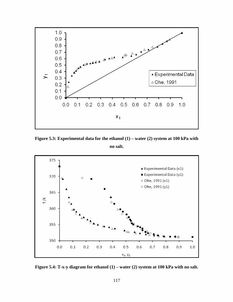
117
Figure 5.3: Experimental data for the ethanol (1) – water (2) system at 100 kPa with
no salt.
Figure 5.4: T-x-y diagram for ethanol (1) – water (2) system at 100 kPa with no salt.
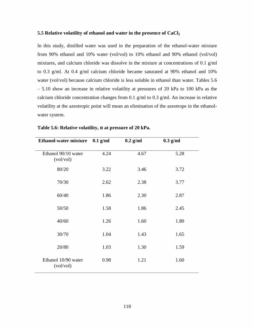
118
5.5 Relative volatility of ethanol and water in the presence of CaCl2
In this study, distilled water was used in the preparation of the ethanol-water mixture
from 90% ethanol and 10% water (vol/vol) to 10% ethanol and 90% ethanol (vol/vol)
mixtures, and calcium chloride was dissolve in the mixture at concentrations of 0.1 g/ml
to 0.3 g/ml. At 0.4 g/ml calcium chloride became saturated at 90% ethanol and 10%
water (vol/vol) because calcium chloride is less soluble in ethanol than water. Tables 5.6
– 5.10 show an increase in relative volatility at pressures of 20 kPa to 100 kPa as the
calcium chloride concentration changes from 0.1 g/ml to 0.3 g/ml. An increase in relative
volatility at the azeotropic point will mean an elimination of the azeotrope in the ethanol-
water system.
Table 5.6: Relative volatility, α at pressure of 20 kPa.
Ethanol-water mixture 0.1 g/ml 0.2 g/ml 0.3 g/ml
Ethanol 90/10 water
(vol/vol)
4.24 4.67 5.28
80/20 3.22 3.46 3.72
70/30 2.62 2.38 3.77
60/40 1.86 2.30 2.87
50/50 1.58 1.86 2.45
40/60 1.26 1.60 1.80
30/70 1.04 1.43 1.65
20/80 1.03 1.30 1.59
Ethanol 10/90 water
(vol/vol)
0.98 1.21 1.60
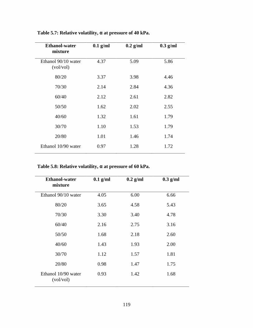
119
Table 5.7: Relative volatility, α at pressure of 40 kPa.
Ethanol-water
mixture
0.1 g/ml 0.2 g/ml 0.3 g/ml
Ethanol 90/10 water
(vol/vol)
4.37 5.09 5.86
80/20 3.37 3.98 4.46
70/30 2.14 2.84 4.36
60/40 2.12 2.61 2.82
50/50 1.62 2.02 2.55
40/60 1.32 1.61 1.79
30/70 1.10 1.53 1.79
20/80 1.01 1.46 1.74
Ethanol 10/90 water 0.97 1.28 1.72
Table 5.8: Relative volatility, α at pressure of 60 kPa.
Ethanol-water
mixture
0.1 g/ml 0.2 g/ml 0.3 g/ml
Ethanol 90/10 water 4.05 6.00 6.66
80/20 3.65 4.58 5.43
70/30 3.30 3.40 4.78
60/40 2.16 2.75 3.16
50/50 1.68 2.18 2.60
40/60 1.43 1.93 2.00
30/70 1.12 1.57 1.81
20/80 0.98 1.47 1.75
Ethanol 10/90 water
(vol/vol)
0.93 1.42 1.68
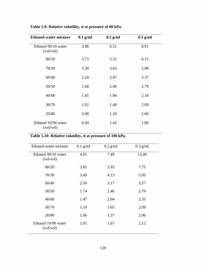
120
Table 5.9: Relative volatility, α at pressure of 80 kPa.
Ethanol-water mixture 0.1 g/ml 0.2 g/ml 0.3 g/ml
Ethanol 90/10 water
(vol/vol)
3.98 6.51 8.91
80/20 3.73 5.32 6.15
70/30 3.39 3.63 5.08
60/40 2.24 2.87 3.37
50/50 1.68 2.40 2.79
40/60 1.45 1.94 2.18
30/70 1.02 1.49 2.09
20/80 0.98 1.59 2.00
Ethanol 10/90 water
(vol/vol)
0.94 1.42 1.89
Table 5.10: Relative volatility, α at pressure of 100 kPa.
Ethanol-water mixture 0.1 g/ml 0.2 g/ml 0.3 g/ml
Ethanol 90/10 water
(vol/vol)
4.01 7.49 13.40
80/20 3.81 5.93 7.75
70/30 3.49 4.13 5.95
60/40 2.50 3.17 3.57
50/50 1.74 2.46 2.79
40/60 1.47 2.04 2.33
30/70 1.10 1.65 2.09
20/80 1.06 1.57 2.06
Ethanol 10/90 water
(vol/vol)
1.01 1.67 2.12
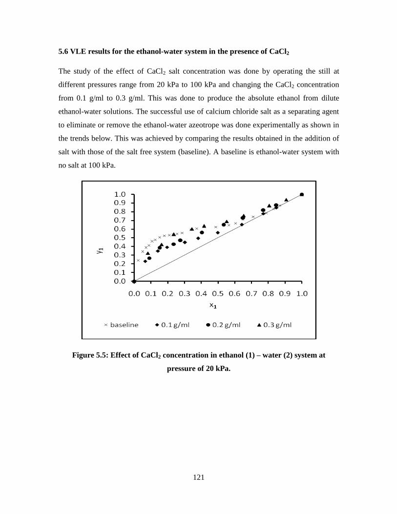
121
5.6 VLE results for the ethanol-water system in the presence of CaCl2
The study of the effect of CaCl2 salt concentration was done by operating the still at
different pressures range from 20 kPa to 100 kPa and changing the CaCl2 concentration
from 0.1 g/ml to 0.3 g/ml. This was done to produce the absolute ethanol from dilute
ethanol-water solutions. The successful use of calcium chloride salt as a separating agent
to eliminate or remove the ethanol-water azeotrope was done experimentally as shown in
the trends below. This was achieved by comparing the results obtained in the addition of
salt with those of the salt free system (baseline). A baseline is ethanol-water system with
no salt at 100 kPa.
Figure 5.5: Effect of CaCl2 concentration in ethanol (1) – water (2) system at
pressure of 20 kPa.

122
Figure 5.6: Effect of CaCl2 concentration in ethanol (1) – water (2) system at
pressure of 40 kPa.
Figure 5.7: Effect of CaCl2 concentration in ethanol (1) – water (2) system at
pressure of 60 kPa.
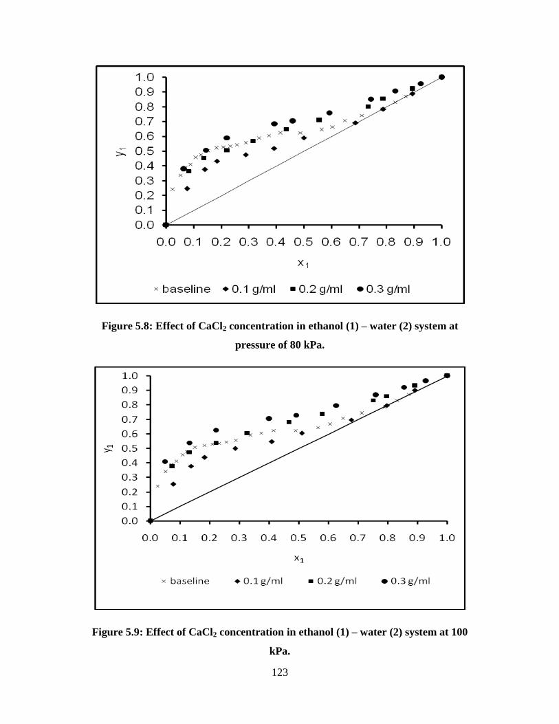
123
Figure 5.8: Effect of CaCl2 concentration in ethanol (1) – water (2) system at
pressure of 80 kPa.
Figure 5.9: Effect of CaCl2 concentration in ethanol (1) – water (2) system at 100
kPa.
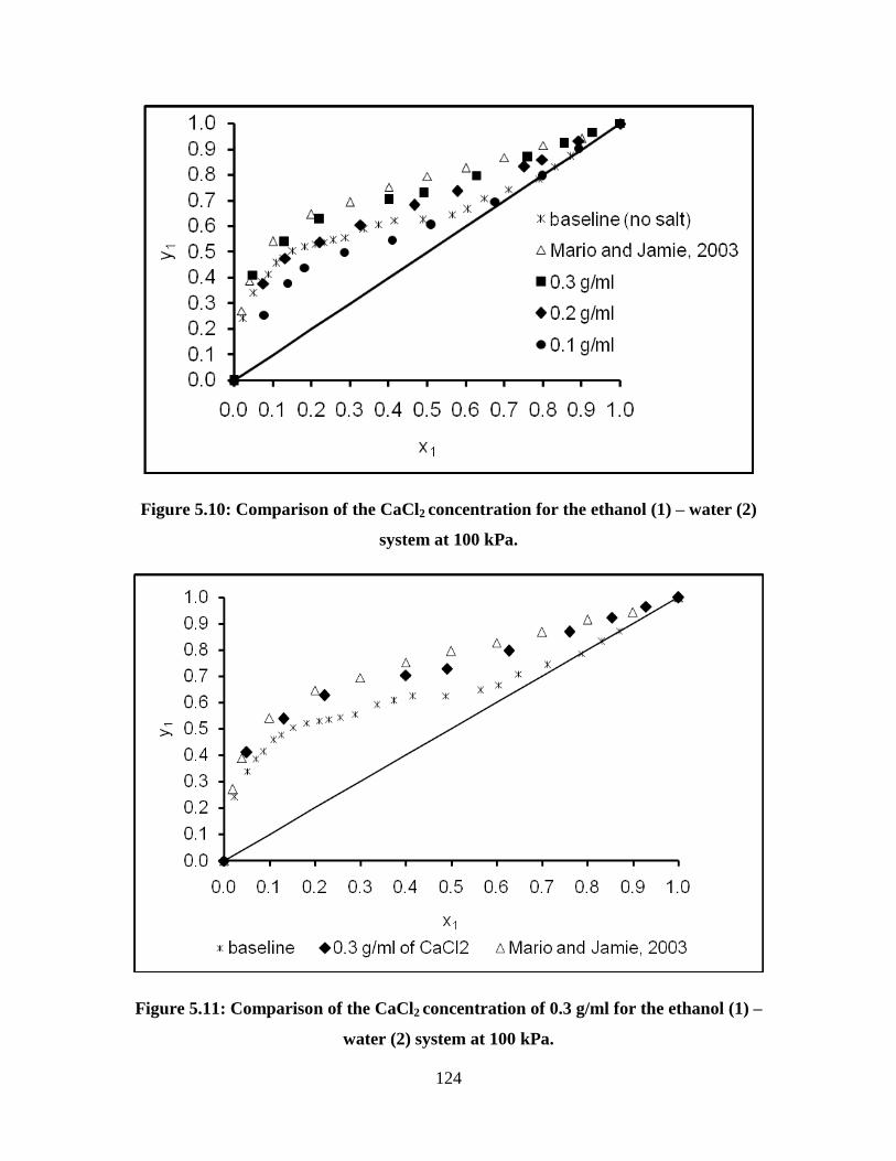
124
Figure 5.10: Comparison of the CaCl2 concentration for the ethanol (1) – water (2)
system at 100 kPa.
Figure 5.11: Comparison of the CaCl2 concentration of 0.3 g/ml for the ethanol (1) –
water (2) system at 100 kPa.
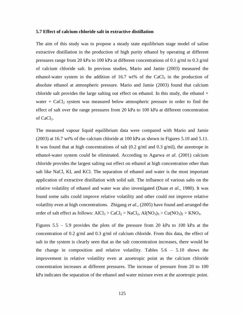
125
5.7 Effect of calcium chloride salt in extractive distillation
The aim of this study was to propose a steady state equilibrium stage model of saline
extractive distillation in the production of high purity ethanol by operating at different
pressures range from 20 kPa to 100 kPa at different concentrations of 0.1 g/ml to 0.3 g/ml
of calcium chloride salt. In previous studies, Mario and Jamie (2003) measured the
ethanol-water system in the addition of 16.7 wt% of the CaCl2 in the production of
absolute ethanol at atmospheric pressure. Mario and Jamie (2003) found that calcium
chloride salt provides the large salting out effect on ethanol. In this study, the ethanol +
water + CaCl2 system was measured below atmospheric pressure in order to find the
effect of salt over the range pressures from 20 kPa to 100 kPa at different concentration
of CaCl2.
The measured vapour liquid equilibrium data were compared with Mario and Jamie
(2003) at 16.7 wt% of the calcium chloride at 100 kPa as shown in Figures 5.10 and 5.11.
It was found that at high concentrations of salt (0.2 g/ml and 0.3 g/ml), the azeotrope in
ethanol-water system could be eliminated. According to Agarwa et al. (2001) calcium
chloride provides the largest salting out effect on ethanol at high concentration other than
salt like NaCl, KI, and KCl. The separation of ethanol and water is the most important
application of extractive distillation with solid salt. The influence of various salts on the
relative volatility of ethanol and water was also investigated (Duan et al., 1980). It was
found some salts could improve relative volatility and other could not improve relative
volatility even at high concentrations. Zhigang et al., (2005) have found and arranged the
order of salt effect as follows: AlCl3 > CaCl2 > NaCl2, Al(NO3)3 > Cu(NO3)2 > KNO3.
Figures 5.5 – 5.9 provides the plots of the pressure from 20 kPa to 100 kPa at the
concentration of 0.2 g/ml and 0.3 g/ml of calcium chloride. From this data, the effect of
salt in the system is clearly seen that as the salt concentration increases, there would be
the change in composition and relative volatility. Tables 5.6 – 5.10 shows the
improvement in relative volatility even at azoetropic point as the calcium chloride
concentration increases at different pressures. The increase of pressure from 20 to 100
kPa indicates the separation of the ethanol and water mixture even at the azoetropic point.
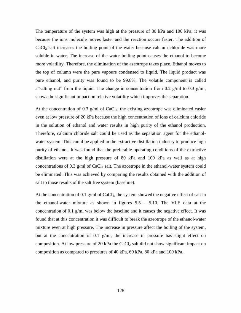
126
The temperature of the system was high at the pressure of 80 kPa and 100 kPa; it was
because the ions molecule moves faster and the reaction occurs faster. The addition of
CaCl2 salt increases the boiling point of the water because calcium chloride was more
soluble in water. The increase of the water boiling point causes the ethanol to become
more volatility. Therefore, the elimination of the azeotrope takes place. Ethanol moves to
the top of column were the pure vapours condensed to liquid. The liquid product was
pure ethanol, and purity was found to be 99.8%. The volatile component is called
a“salting out” from the liquid. The change in concentration from 0.2 g/ml to 0.3 g/ml,
shows the significant impact on relative volatility which improves the separation.
At the concentration of 0.3 g/ml of CaCl2, the existing azeotrope was eliminated easier
even at low pressure of 20 kPa because the high concentration of ions of calcium chloride
in the solution of ethanol and water results in high purity of the ethanol production.
Therefore, calcium chloride salt could be used as the separation agent for the ethanol-
water system. This could be applied in the extractive distillation industry to produce high
purity of ethanol. It was found that the preferable operating conditions of the extractive
distillation were at the high pressure of 80 kPa and 100 kPa as well as at high
concentrations of 0.3 g/ml of CaCl2 salt. The azoetrope in the ethanol-water system could
be eliminated. This was achieved by comparing the results obtained with the addition of
salt to those results of the salt free system (baseline).
At the concentration of 0.1 g/ml of CaCl2, the system showed the negative effect of salt in
the ethanol-water mixture as shown in figures 5.5 – 5.10. The VLE data at the
concentration of 0.1 g/ml was below the baseline and it causes the negative effect. It was
found that at this concentration it was difficult to break the azeotrope of the ethanol-water
mixture even at high pressure. The increase in pressure affect the boiling of the system,
but at the concentration of 0.1 g/ml, the increase in pressure has slight effect on
composition. At low pressure of 20 kPa the CaCl2 salt did not show significant impact on
composition as compared to pressures of 40 kPa, 60 kPa, 80 kPa and 100 kPa.
127
5.8 Calcium chloride as an extractive agent
Calcium chloride salt is a molecular solid, in which the individual molecules are held
together by relatively weak intermolecular forces. When calcium chloride dissolves in the
ethanol-water mixture, the weak bonds between the individual CaCl2 molecules are
broken and these molecules are released into the solution. It takes energy to beak the
bonds between the CaCl2 molecules, as well as the hydrogen bonds in ethanol-water
mixture. Hydrogen bonds in ethanol and water were disrupted by the addition of calcium
chloride. As calcium chloride salt dissolves in the ethanol-water mixture, energy is given
off. The slightly polar calcium chloride molecules form intermolecular bonds with polar
ethanol and water molecules. The weak bonds formed between the solute and the solvent
compensate for the energy needed to disrupt the structure of both the pure solute and the
solvent. Calcium chloride salt completely dissolved in the ethanol-water mixture at the
concentrations of 0.1 g/ml to 0.3 g/ml and it became saturated at the concentration of 0.4
g/ml.
To overcome the difficulty of eliminating existing azeotrope in the ethanol-water system,
the use of solid salts instead of liquid separating agents has been gaining more attention
in the past few years (Zhigang et al., 2005). By using salt as an extractive agent, the
extractive distillation has the advantages of producing a solvent-free extract at the top of
the column and requires no additional separating column. This consumes less energy
when compared to conventional methods of extractive distillation. In addition, the
calcium chloride salt is a common salt, which is much cheaper than liquid solvents. Thus,
it is unnecessary to recover the salt (CaCl2) at the bottom of distillation column.
It is known that when a salt is dissolved in a solution, it dissociates into ions so as to
exhibit preferential salvation by one of the solvents (usually less volatile) and salting-out
of the other solvent (usually more volatile), as shown in experimental behavior of the
ethanol-water system in the presence of calcium chloride salt. It may also happen that
only a part of it dissociates leaving some un-dissociated molecules in the solution.
Consequently the interaction forces between un-dissociates salt molecules, ion-molecules
and ion-ion can coexist (Mario and Jamie, 2003). The strength of interaction forces
depends on the configuration of ions and molecules, polarities of molecules, ionic
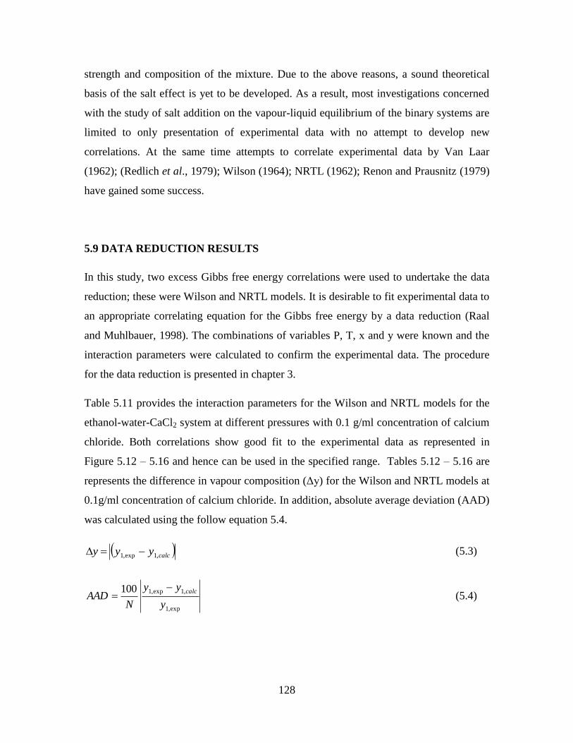
128
strength and composition of the mixture. Due to the above reasons, a sound theoretical
basis of the salt effect is yet to be developed. As a result, most investigations concerned
with the study of salt addition on the vapour-liquid equilibrium of the binary systems are
limited to only presentation of experimental data with no attempt to develop new
correlations. At the same time attempts to correlate experimental data by Van Laar
(1962); (Redlich et al., 1979); Wilson (1964); NRTL (1962); Renon and Prausnitz (1979)
have gained some success.
5.9 DATA REDUCTION RESULTS
In this study, two excess Gibbs free energy correlations were used to undertake the data
reduction; these were Wilson and NRTL models. It is desirable to fit experimental data to
an appropriate correlating equation for the Gibbs free energy by a data reduction (Raal
and Muhlbauer, 1998). The combinations of variables P, T, x and y were known and the
interaction parameters were calculated to confirm the experimental data. The procedure
for the data reduction is presented in chapter 3.
Table 5.11 provides the interaction parameters for the Wilson and NRTL models for the
ethanol-water-CaCl2 system at different pressures with 0.1 g/ml concentration of calcium
chloride. Both correlations show good fit to the experimental data as represented in
Figure 5.12 – 5.16 and hence can be used in the specified range. Tables 5.12 – 5.16 are
represents the difference in vapour composition (Δy) for the Wilson and NRTL models at
0.1g/ml concentration of calcium chloride. In addition, absolute average deviation (AAD)
was calculated using the follow equation 5.4.
calcyyy ,1exp,1 (5.3)
exp,1
,1exp,1100
y
yy
NAAD
calc (5.4)

129
Table 5.11: Interaction parameter for the Wilson and NRTL models for ethanol (1)
– water (2) system at 0.1 g/ml of CaCl2.
Pressure/ kPa 20 40 60 80 100
Wilson
(12- 11)/J.mol-1
942.20 1137.28 1498.27 1724.17 1943.65
( 21- 22)/J.mol-1
3198.26 3488.61 3811.26 3712.91 3878.13
AAD 0.473 0.37 0.33 0.284 0.422
NRTL
(g12-g11)/J.mol-1
263.28 786.98 1444.32 1886.54 2118.89
(g21-g22)/J.mol-1
4123.32 3163.32 4466.28 4583.63 4095.86
Α 0.45 0.46 0.47 0.46 0.45
AAD 0.279 0.328 0.312 0.285 0.283
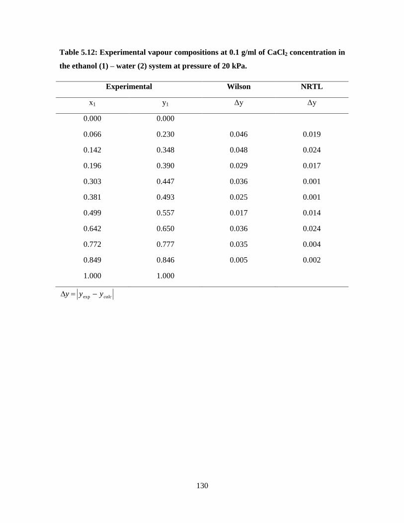
130
Table 5.12: Experimental vapour compositions at 0.1 g/ml of CaCl2 concentration in
the ethanol (1) – water (2) system at pressure of 20 kPa.
Experimental Wilson NRTL
x1 y1 Δy Δy
0.000 0.000
0.066 0.230 0.046 0.019
0.142 0.348 0.048 0.024
0.196 0.390 0.029 0.017
0.303 0.447 0.036 0.001
0.381 0.493 0.025 0.001
0.499 0.557 0.017 0.014
0.642 0.650 0.036 0.024
0.772 0.777 0.035 0.004
0.849 0.846 0.005 0.002
1.000 1.000
calcyyy exp
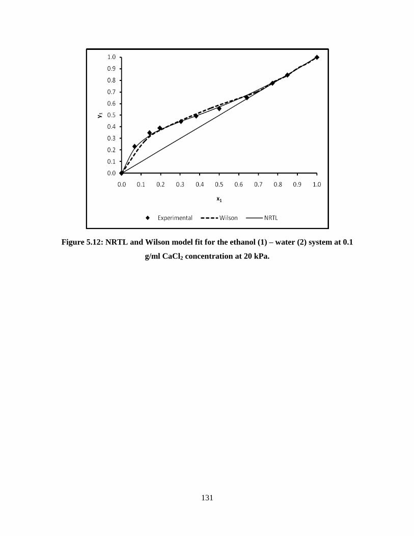
131
Figure 5.12: NRTL and Wilson model fit for the ethanol (1) – water (2) system at 0.1
g/ml CaCl2 concentration at 20 kPa.

132
Table 5.13: Experimental vapour compositions at 0.1 g/ml of CaCl2 concentration in
the ethanol (1) – water (2) system at pressure of 40 kPa.
Experimental Wilson NRTL
x1 y1 Δy Δy
0.000 0.000
0.068 0.241 0.035 0.030
0.142 0.357 0.039 0.033
0.191 0.426 0.015 0.027
0.296 0.472 0.021 0.026
0.398 0.518 0.010 0.023
0.494 0.564 0.014 0.007
0.631 0.652 0.029 0.022
0.781 0.782 0.030 0.002
0.874 0.870 0.009 0.022
1.000 1.000
calcyyy exp

133
Figure 5.13: NRTL and Wilson model fit for the ethanol (1) – water (2) system at 0.1
g/ml CaCl2 concentration at 40 kPa.

134
Table 5.14: Experimental vapour compositions at 0.1 g/ml of CaCl2 concentration in
the ethanol (1) – water (2) system at pressure of 60 kPa.
Experimental Wilson NRTL
x1 y1 Δy Δy
0.000 0.000
0.074 0.246 0.033 0.025
0.141 0.375 0.024 0.030
0.187 0.432 0.030 0.033
0.294 0.473 0.018 0.017
0.391 0.519 0.011 0.021
0.491 0.580 0.011 0.027
0.628 0.654 0.011 0.003
0.789 0.785 0.016 0.004
0.877 0.877 0.017 0.009
1.000 1.000
calcyyy exp
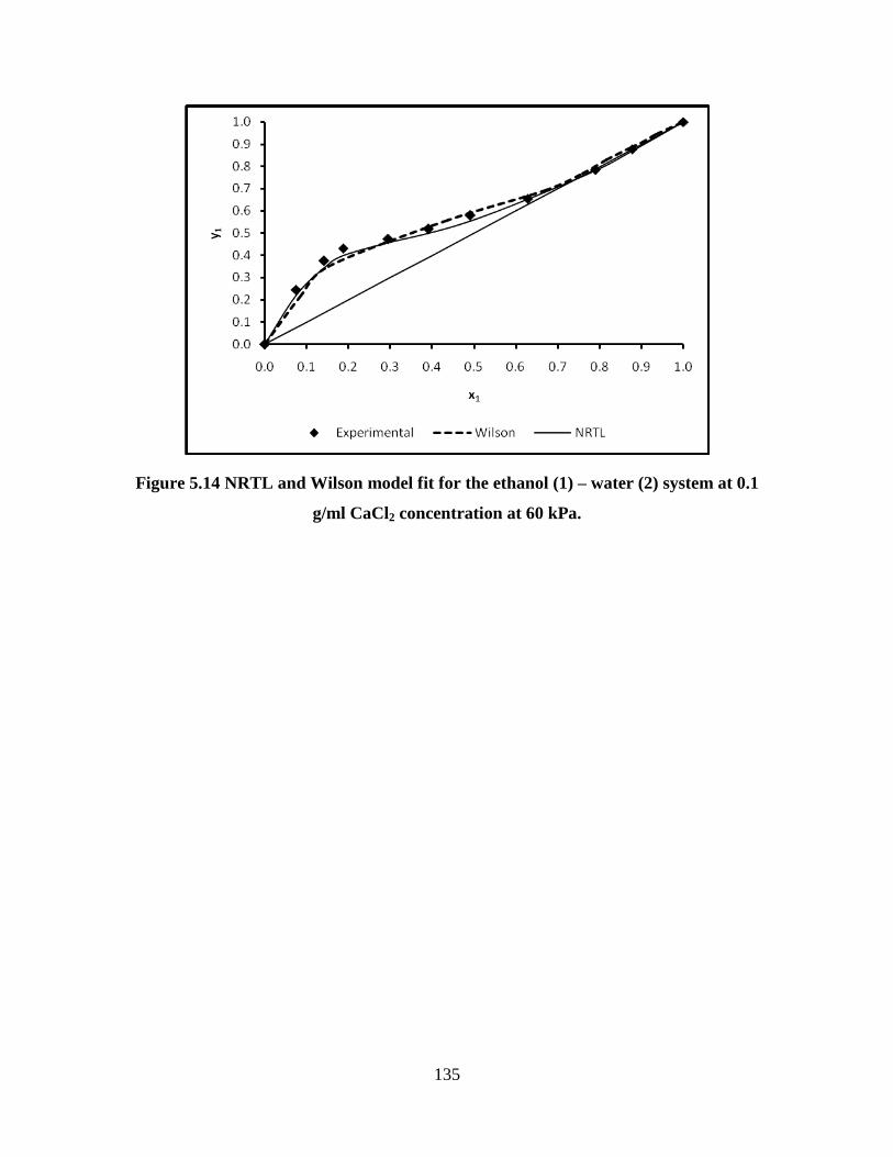
135
Figure 5.14 NRTL and Wilson model fit for the ethanol (1) – water (2) system at 0.1
g/ml CaCl2 concentration at 60 kPa.

136
Table 5.15: Experimental vapour compositions at 0.1 g/ml of CaCl2 concentration in
the ethanol (1) – water (2) system at pressure of 80 kPa.
Experimental Wilson NRTL
x1 y1 Δy Δy
0.000 0.000
0.076 0.247 0.017 0.016
0.140 0.377 0.001 0.034
0.184 0.433 0.048 0.035
0.289 0.477 0.002 0.029
0.392 0.520 0.023 0.024
0.500 0.591 0.030 0.024
0.688 0.693 0.029 0.012
0.788 0.785 0.017 0.002
0.894 0.888 0.015 0.007
1.000 1.000
calcyyy exp

137
Figure 5.15: NRTL and Wilson model fit for the ethanol (1) – water (2) system at 0.1
g/ml CaCl2 concentration at 80 kPa.
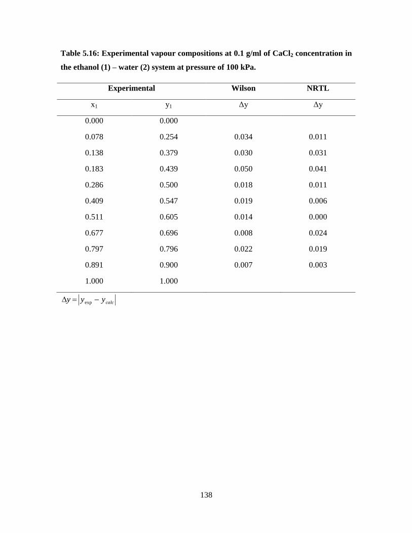
138
Table 5.16: Experimental vapour compositions at 0.1 g/ml of CaCl2 concentration in
the ethanol (1) – water (2) system at pressure of 100 kPa.
Experimental Wilson NRTL
x1 y1 Δy Δy
0.000 0.000
0.078 0.254 0.034 0.011
0.138 0.379 0.030 0.031
0.183 0.439 0.050 0.041
0.286 0.500 0.018 0.011
0.409 0.547 0.019 0.006
0.511 0.605 0.014 0.000
0.677 0.696 0.008 0.024
0.797 0.796 0.022 0.019
0.891 0.900 0.007 0.003
1.000 1.000
calcyyy exp
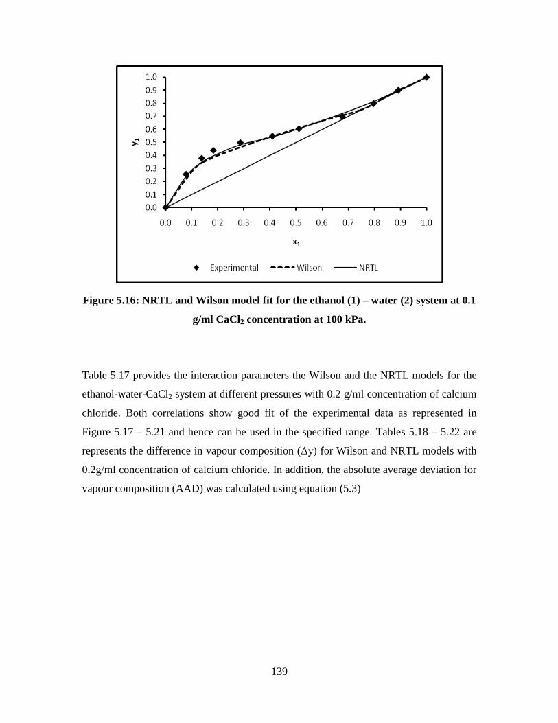
139
Figure 5.16: NRTL and Wilson model fit for the ethanol (1) – water (2) system at 0.1
g/ml CaCl2 concentration at 100 kPa.
Table 5.17 provides the interaction parameters the Wilson and the NRTL models for the
ethanol-water-CaCl2 system at different pressures with 0.2 g/ml concentration of calcium
chloride. Both correlations show good fit of the experimental data as represented in
Figure 5.17 – 5.21 and hence can be used in the specified range. Tables 5.18 – 5.22 are
represents the difference in vapour composition (Δy) for Wilson and NRTL models with
0.2g/ml concentration of calcium chloride. In addition, the absolute average deviation for
vapour composition (AAD) was calculated using equation (5.3)
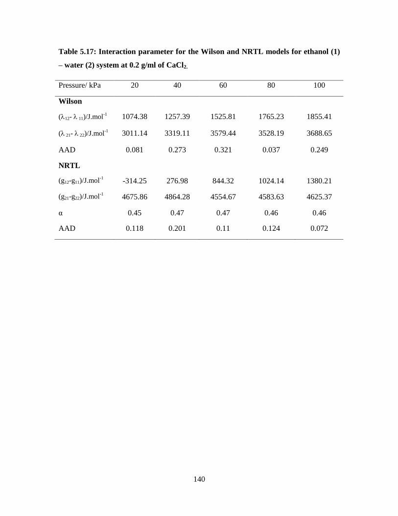
140
Table 5.17: Interaction parameter for the Wilson and NRTL models for ethanol (1)
– water (2) system at 0.2 g/ml of CaCl2.
Pressure/ kPa 20 40 60 80 100
Wilson
(12- 11)/J.mol-1
1074.38 1257.39 1525.81 1765.23 1855.41
( 21- 22)/J.mol-1
3011.14 3319.11 3579.44 3528.19 3688.65
AAD 0.081 0.273 0.321 0.037 0.249
NRTL
(g12-g11)/J.mol-1
-314.25 276.98 844.32 1024.14 1380.21
(g21-g22)/J.mol-1
4675.86 4864.28 4554.67 4583.63 4625.37
α 0.45 0.47 0.47 0.46 0.46
AAD 0.118 0.201 0.11 0.124 0.072

141
Table 5.18: Experimental vapour compositions at 0.2 g/ml of CaCl2 concentration in
the ethanol (1) – water (2) system at pressure of 20 kPa.
Experimental Wilson NRTL
x1 y1 Δy Δy
0.000 0.000
0.090 0.266 0.005 0.010
0.152 0.382 0.001 0.023
0.237 0.426 0.011 0.008
0.277 0.469 0.002 0.015
0.404 0.558 0.005 0.014
0.534 0.646 0.007 0.015
0.650 0.725 0.012 0.002
0.772 0.815 0.011 0.016
0.849 0.872 0.026 0.024
1.000 1.000
calcyyy exp
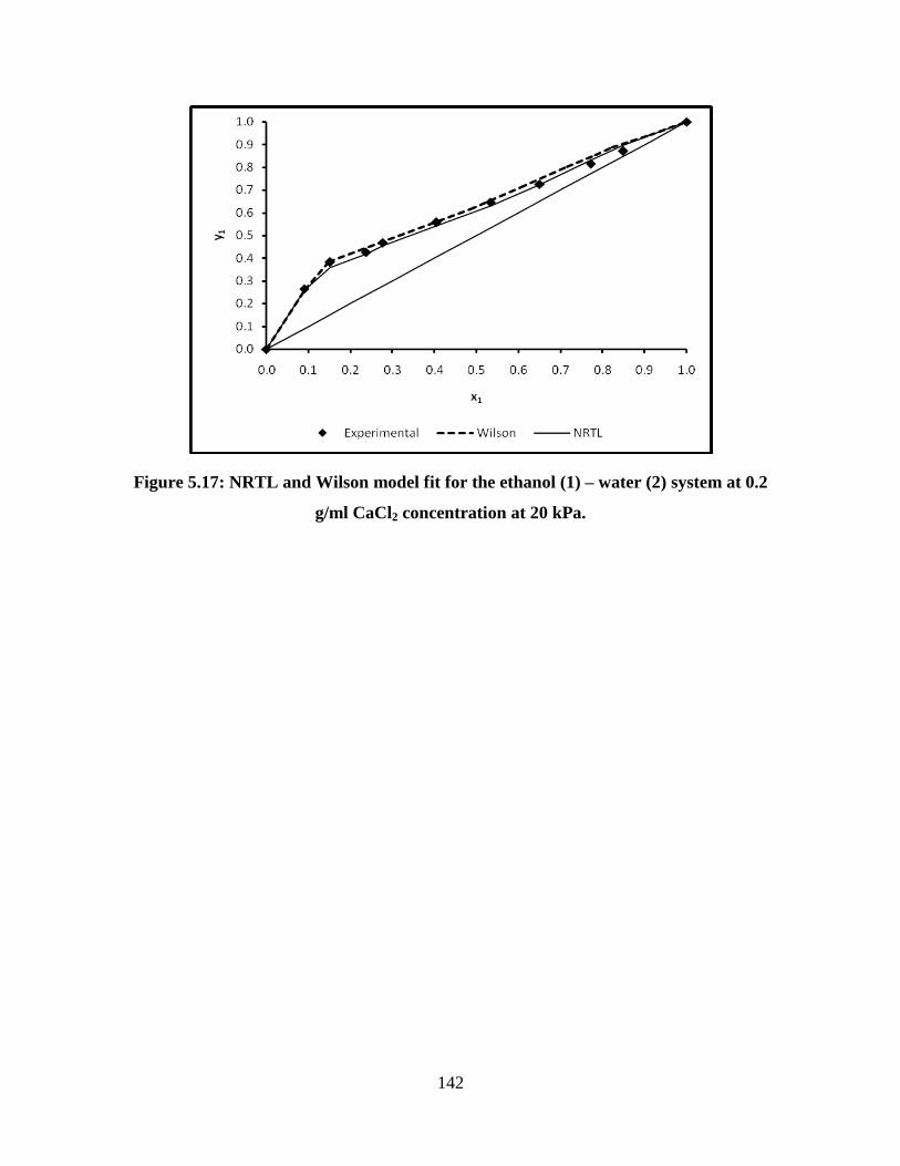
142
Figure 5.17: NRTL and Wilson model fit for the ethanol (1) – water (2) system at 0.2
g/ml CaCl2 concentration at 20 kPa.
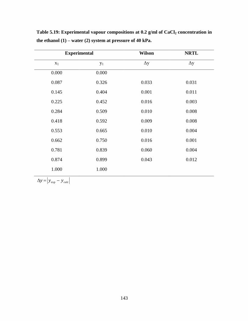
143
Table 5.19: Experimental vapour compositions at 0.2 g/ml of CaCl2 concentration in
the ethanol (1) – water (2) system at pressure of 40 kPa.
Experimental Wilson NRTL
x1 y1 Δy Δy
0.000 0.000
0.087 0.326 0.033 0.031
0.145 0.404 0.001 0.011
0.225 0.452 0.016 0.003
0.284 0.509 0.010 0.008
0.418 0.592 0.009 0.008
0.553 0.665 0.010 0.004
0.662 0.750 0.016 0.001
0.781 0.839 0.060 0.004
0.874 0.899 0.043 0.012
1.000 1.000
calcyyy exp
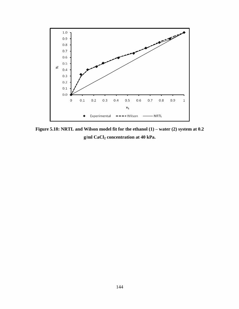
144
Figure 5.18: NRTL and Wilson model fit for the ethanol (1) – water (2) system at 0.2
g/ml CaCl2 concentration at 40 kPa.

145
Table 5.20: Experimental vapour compositions at 0.2 g/ml of CaCl2 concentration in
the ethanol (1) – water (2) system at pressure of 60 kPa.
Experimental Wilson NRTL
x1 y1 Δy Δy
0.000 0.000
0.085 0.359 0.001 0.014
0.140 0.427 0.002 0.003
0.219 0.488 0.053 0.008
0.301 0.542 0.037 0.002
0.431 0.623 0.024 0.013
0.523 0.680 0.018 0.021
0.694 0.781 0.016 0.018
0.789 0.846 0.060 0.015
0.877 0.910 0.011 0.007
1.000 1.000
calcyyy exp
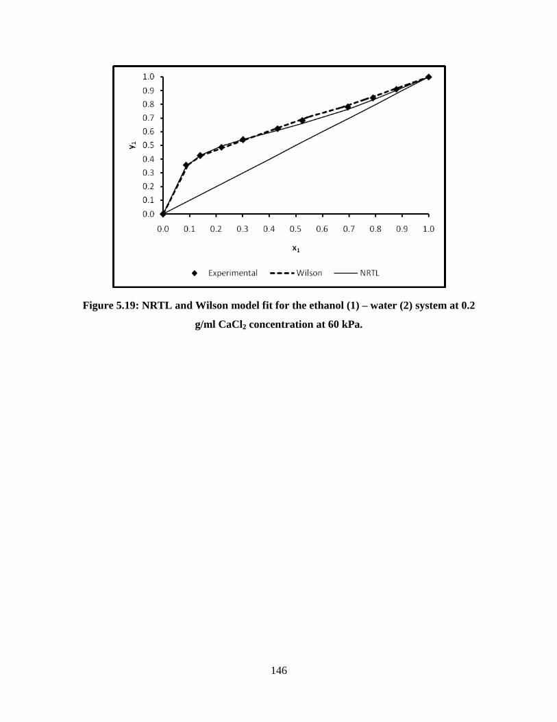
146
Figure 5.19: NRTL and Wilson model fit for the ethanol (1) – water (2) system at 0.2
g/ml CaCl2 concentration at 60 kPa.

147
Table 5.21: Experimental vapour compositions at 0.2 g/ml of CaCl2 concentration in
the ethanol (1) – water (2) system at pressure of 80 kPa.
Experimental Wilson NRTL
x1 y1 Δy Δy
0.000 0.000
0.081 0.366 0.003 0.017
0.136 0.456 0.025 0.018
0.222 0.508 0.003 0.001
0.315 0.569 0.099 0.006
0.436 0.649 0.010 0.018
0.557 0.710 0.026 0.016
0.733 0.804 0.027 0.012
0.788 0.855 0.037 0.025
0.894 0.903 0.039 0.013
1.000 1.000
calcyyy exp
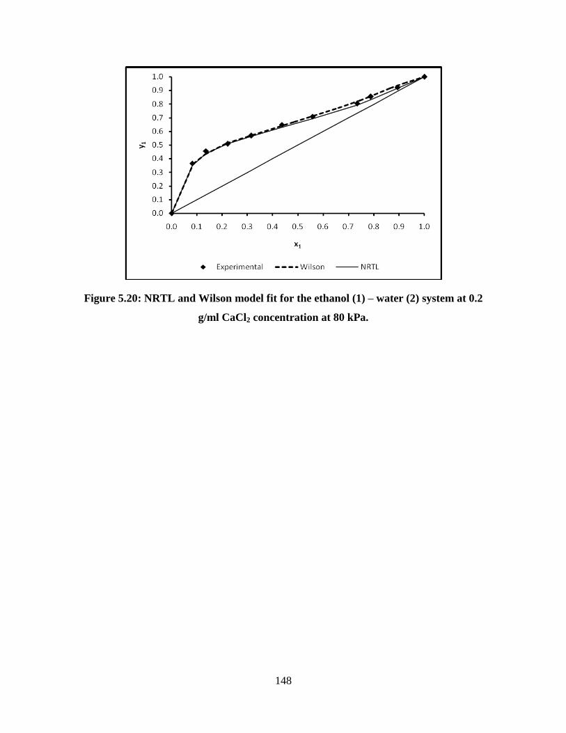
148
Figure 5.20: NRTL and Wilson model fit for the ethanol (1) – water (2) system at 0.2
g/ml CaCl2 concentration at 80 kPa.

149
Table 5.22: Experimental vapour compositions at 0.2 g/ml of CaCl2 concentration in
the ethanol (1) – water (2) system at pressure of 100 kPa.
Experimental Wilson NRTL
x1 y1 Δy Δy
0.000 0.000
0.075 0.377 0.045 0.012
0.132 0.475 0.027 0.005
0.221 0.540 0.009 0.010
0.327 0.606 0.038 0.004
0.467 0.683 0.029 0.009
0.578 0.737 0.027 0.008
0.750 0.832 0.030 0.001
0.797 0.860 0.028 0.004
0.891 0.932 0.010 0.007
1.000 1.000
calcyyy exp

150
Figure 5.21: NRTL and Wilson model fit for the ethanol (1) – water (2) system at 0.2
g/ml CaCl2 concentration at 100 kPa.
Table 5.23 provides the interaction parameters of the Wilson and the NRTL models for
the ethanol-water-CaCl2 system at different pressures with 0.3 g/ml concentration of
calcium chloride. Both correlations show good fit to the experimental data as represented
in Figures 5.22 – 5.26 and hence can be used in the specified range. Tables 5.24 – 5.28
are represents the difference in vapour composition (Δy) for Wilson and NRTL models
with 0.3 g/ml concentration of calcium chloride. In addition, the absolute average
deviation for vapour composition (AAD) was calculated using equation (5.3)
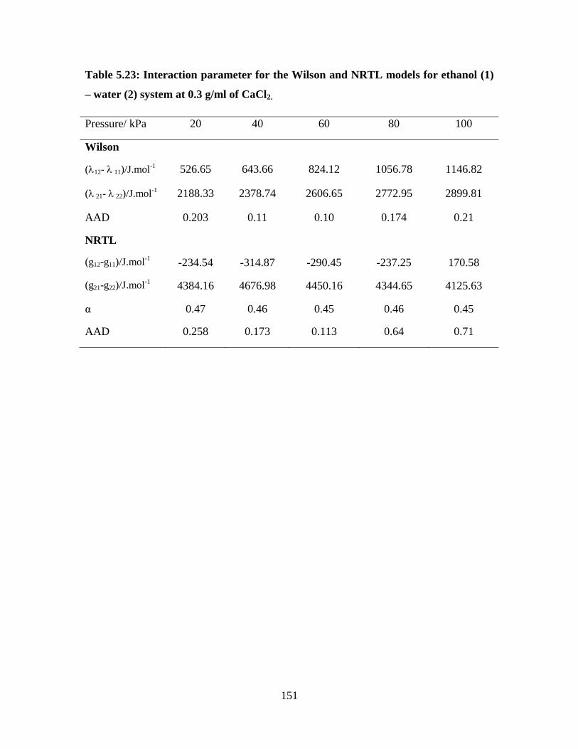
151
Table 5.23: Interaction parameter for the Wilson and NRTL models for ethanol (1)
– water (2) system at 0.3 g/ml of CaCl2.
Pressure/ kPa 20 40 60 80 100
Wilson
(12- 11)/J.mol-1
526.65 643.66 824.12 1056.78 1146.82
( 21- 22)/J.mol-1
2188.33 2378.74 2606.65 2772.95 2899.81
AAD 0.203 0.11 0.10 0.174 0.21
NRTL
(g12-g11)/J.mol-1
-234.54 -314.87 -290.45 -237.25 170.58
(g21-g22)/J.mol-1
4384.16 4676.98 4450.16 4344.65 4125.63
α 0.47 0.46 0.45 0.46 0.45
AAD 0.258 0.173 0.113 0.64 0.71

152
Table 5.24: Experimental vapour compositions at 0.3 g/ml of CaCl2 concentration in
the ethanol (1) – water (2) system at pressure of 20 kPa.
Experimental Wilson NRTL
x1 y1 Δy Δy
0.000 0.000
0.083 0.322 0.001 0.013
0.164 0.422 0.021 0.043
0.237 0.540 0.007 0.014
0.345 0.602 0.039 0.007
0.417 0.637 0.024 0.004
0.552 0.689 0.012 0.001
0.653 0.756 0.025 0.002
0.807 0.869 0.009 0.000
0.907 0.940 0.003 0.001
1.000 1.000
calcyyy exp

153
Figure 5.22: NRTL and Wilson model fit for the ethanol (1) – water (2) system at 0.3
g/ml CaCl2 concentration at 20 kPa.
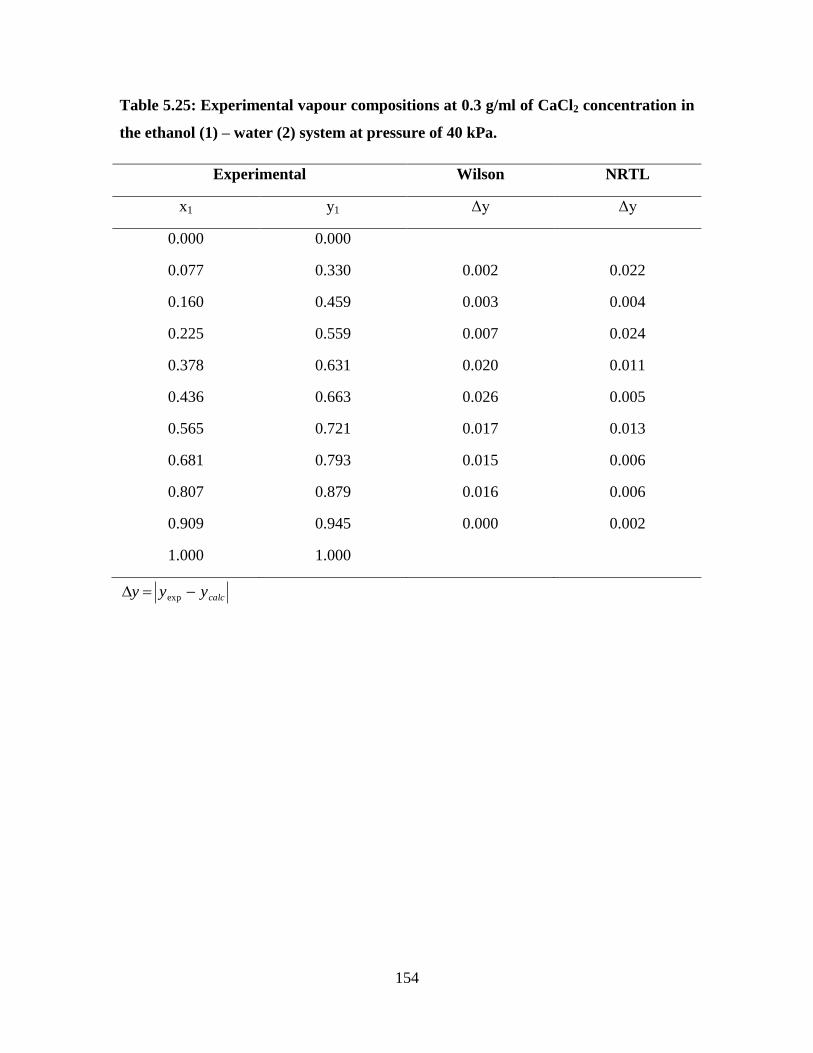
154
Table 5.25: Experimental vapour compositions at 0.3 g/ml of CaCl2 concentration in
the ethanol (1) – water (2) system at pressure of 40 kPa.
Experimental Wilson NRTL
x1 y1 Δy Δy
0.000 0.000
0.077 0.330 0.002 0.022
0.160 0.459 0.003 0.004
0.225 0.559 0.007 0.024
0.378 0.631 0.020 0.011
0.436 0.663 0.026 0.005
0.565 0.721 0.017 0.013
0.681 0.793 0.015 0.006
0.807 0.879 0.016 0.006
0.909 0.945 0.000 0.002
1.000 1.000
calcyyy exp
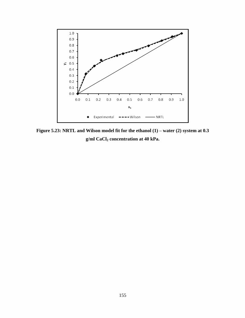
155
Figure 5.23: NRTL and Wilson model fit for the ethanol (1) – water (2) system at 0.3
g/ml CaCl2 concentration at 40 kPa.

156
Table 5.26: Experimental vapour compositions at 0.3 g/ml of CaCl2 concentration in
the ethanol (1) – water (2) system at pressure of 60 kPa.
Experimental Wilson NRTL
x1 y1 Δy Δy
0.000 0.000
0.071 0.337 0.005 0.006
0.145 0.480 0.006 0.024
0.219 0.573 0.005 0.009
0.382 0.662 0.017 0.007
0.449 0.679 0.018 0.000
0.578 0.732 0.027 0.005
0.715 0.819 0.026 0.021
0.826 0.893 0.019 0.021
0.923 0.952 0.004 0.010
1.000 1.000
calcyyy exp

157
Figure 5.24: NRTL and Wilson model fit for the ethanol (1) – water (2) system at 0.3
g/ml CaCl2 concentration at 60 kPa.

158
Table 5.27: Experimental vapour compositions at 0.3 g/ml of CaCl2 concentration in
the ethanol (1) – water (2) system at pressure of 80 kPa.
Experimental Wilson NRTL
x1 y1 Δy Δy
0.000 0.000
0.064 0.379 0.004 0.011
0.144 0.508 0.020 0.007
0.222 0.591 0.005 0.018
0.395 0.687 0.004 0.012
0.460 0.704 0.043 0.016
0.592 0.760 0.022 0.005
0.743 0.853 0.009 0.018
0.832 0.908 0.005 0.019
0.924 0.958 0.006 0.014
1.000 1.000
calcyyy exp
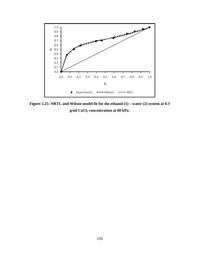
159
Figure 5.25: NRTL and Wilson model fit for the ethanol (1) – water (2) system at 0.3
g/ml CaCl2 concentration at 80 kPa.

160
Table 5.28: Experimental vapour compositions at 0.3 g/ml of CaCl2 concentration in
the ethanol (1) – water (2) system at pressure of 100 kPa.
Experimental Wilson NRTL
x1 y1 Δy Δy
0.000 0.000
0.049 0.411 0.019 0.007
0.131 0.539 0.008 0.011
0.221 0.628 0.006 0.006
0.400 0.704 0.047 0.010
0.491 0.729 0.015 0.016
0.627 0.797 0.004 0.002
0.760 0.869 0.013 0.011
0.854 0.923 0.005 0.006
1.000 1.000
calcyyy exp
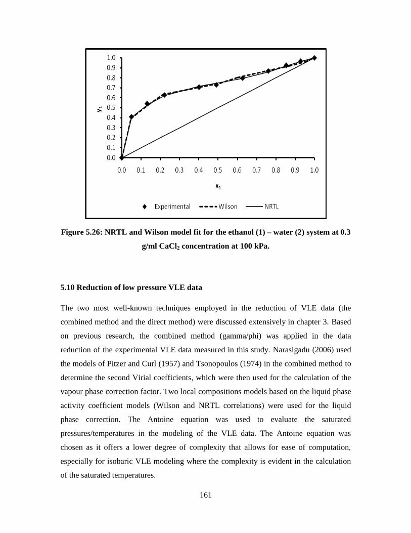
161
Figure 5.26: NRTL and Wilson model fit for the ethanol (1) – water (2) system at 0.3
g/ml CaCl2 concentration at 100 kPa.
5.10 Reduction of low pressure VLE data
The two most well-known techniques employed in the reduction of VLE data (the
combined method and the direct method) were discussed extensively in chapter 3. Based
on previous research, the combined method (gamma/phi) was applied in the data
reduction of the experimental VLE data measured in this study. Narasigadu (2006) used
the models of Pitzer and Curl (1957) and Tsonopoulos (1974) in the combined method to
determine the second Virial coefficients, which were then used for the calculation of the
vapour phase correction factor. Two local compositions models based on the liquid phase
activity coefficient models (Wilson and NRTL correlations) were used for the liquid
phase correction. The Antoine equation was used to evaluate the saturated
pressures/temperatures in the modeling of the VLE data. The Antoine equation was
chosen as it offers a lower degree of complexity that allows for ease of computation,
especially for isobaric VLE modeling where the complexity is evident in the calculation
of the saturated temperatures.
162
In this study, the salt containing liquid mixture was treated as pseudo-binary system with
Wilson and NRTL correlation. Tables 5.11, 5.17 and 5.23 were shows interaction
parameters of the Wilson and NRTL models for the ethanol-water-CaCl2 systemat
different pressures and different concentrations. The MATLAB program was used to
determine the interaction parameters. The data regression program was written in
MATLAB, which offered a variety of built-in optimisation functions. For this work the
fminsearch function was chosen, which finds the minimum of an unconstrained
multivariable function. These models were used at different pressures of 20 kPa to 100
kPa and at the different concentrations of 0.1 g/ml to 0.3 g/ml of calcium chloride salt.
The successful use of these two models is shown from Figures 5.12 – 5.26. Figures 5.12 –
5.16 were shows the result of the models at low concentration of 0.1 g/ml, and from
figure 5.17 to figure 5.21 shows the result of the models at medium concentration of 0.2
g/ml and final from figure 5.22 to figure 5.26 shows the result of the models at high
concentration of 0.3 g/ml.
5.11 PERVAPORATION RESULTS
The cylindrical pervaporation cell was constructed, commission and used to perform the
separation of the ethanol-water system at different temperature and different pressures to
produce high purity ethanol. The pervaporation membrane has the advantage for the
direct separation and it does not need the third component to shift or break the azoetrope.
The pervaporation cell produced the following results confirming that the composite flat
sheet membrane can be used for the production of high purity ethanol. The optimum
temperature and pressure was found.
Ethanol purity
Ethanol purity was tested on the retentate stream for the refractive index after it was
diluted with distilled water. This was done at different temperatures and compared with
literature values taken from Weast (1983-1984). The water was collected from the
permeate tank and the refractive index was tested and compared with literature values
from Weast (1983-1984). The desired product (ethanol) was found at retentate stream,
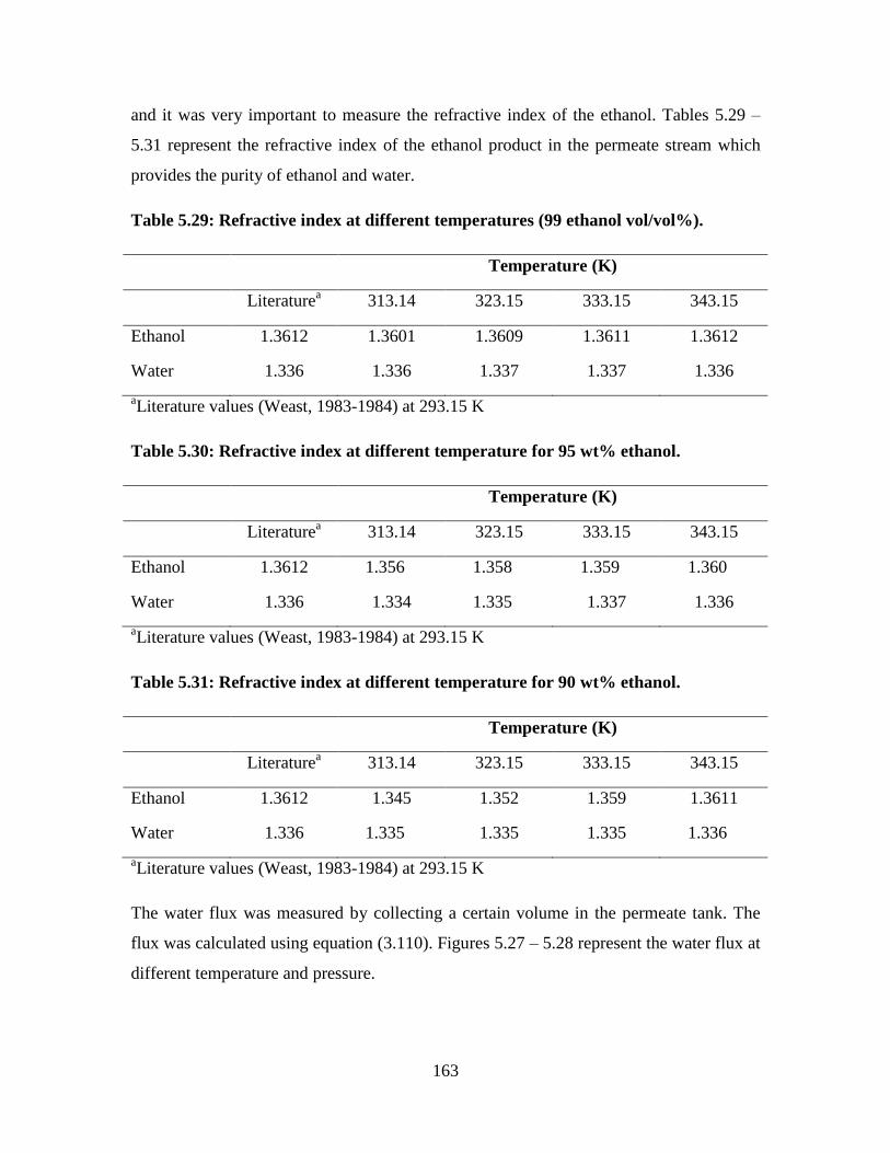
163
and it was very important to measure the refractive index of the ethanol. Tables 5.29 –
5.31 represent the refractive index of the ethanol product in the permeate stream which
provides the purity of ethanol and water.
Table 5.29: Refractive index at different temperatures (99 ethanol vol/vol%).
Temperature (K)
Literaturea 313.14 323.15 333.15 343.15
Ethanol 1.3612 1.3601 1.3609 1.3611 1.3612
Water 1.336 1.336 1.337 1.337 1.336
aLiterature values (Weast, 1983-1984) at 293.15 K
Table 5.30: Refractive index at different temperature for 95 wt% ethanol.
Temperature (K)
Literaturea 313.14 323.15 333.15 343.15
Ethanol 1.3612 1.356 1.358 1.359 1.360
Water 1.336 1.334 1.335 1.337 1.336
aLiterature values (Weast, 1983-1984) at 293.15 K
Table 5.31: Refractive index at different temperature for 90 wt% ethanol.
Temperature (K)
Literaturea 313.14 323.15 333.15 343.15
Ethanol 1.3612 1.345 1.352 1.359 1.3611
Water 1.336 1.335 1.335 1.335 1.336
aLiterature values (Weast, 1983-1984) at 293.15 K
The water flux was measured by collecting a certain volume in the permeate tank. The
flux was calculated using equation (3.110). Figures 5.27 – 5.28 represent the water flux at
different temperature and pressure.
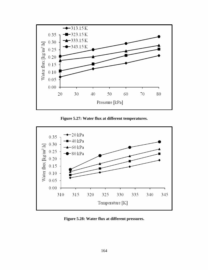
164
Figure 5.27: Water flux at different temperatures.
Figure 5.28: Water flux at different pressures.
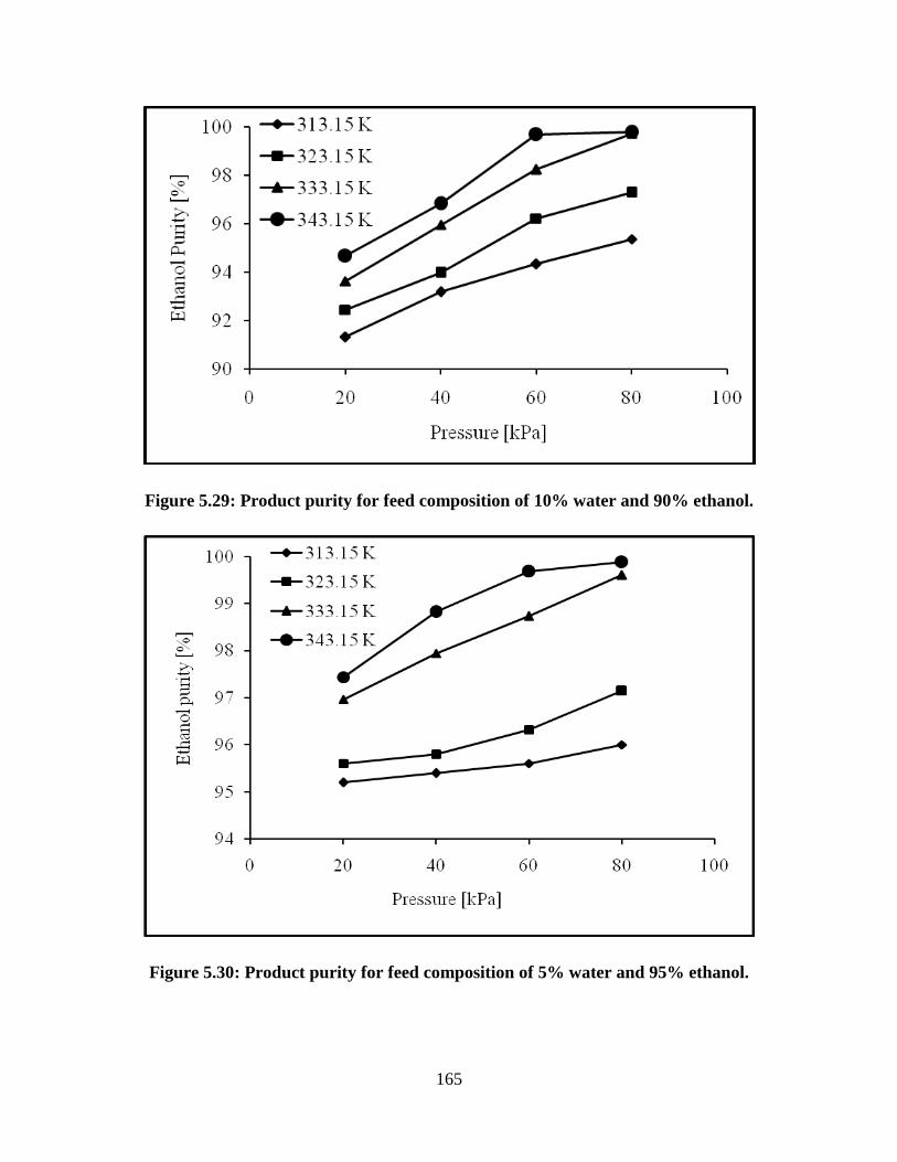
165
Figure 5.29: Product purity for feed composition of 10% water and 90% ethanol.
Figure 5.30: Product purity for feed composition of 5% water and 95% ethanol.
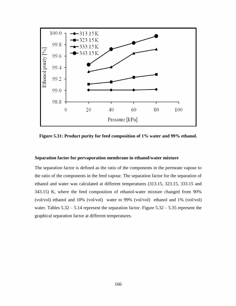
166
Figure 5.31: Product purity for feed composition of 1% water and 99% ethanol.
Separation factor for pervaporation membrane in ethanol/water mixture
The separation factor is defined as the ratio of the components in the permeate vapour to
the ratio of the components in the feed vapour. The separation factor for the separation of
ethanol and water was calculated at different temperatures (313.15, 323.15, 333.15 and
343.15) K, where the feed composition of ethanol-water mixture changed from 90%
(vol/vol) ethanol and 10% (vol/vol) water to 99% (vol/vol) ethanol and 1% (vol/vol)
water. Tables 5.32 – 5.14 represent the separation factor. Figure 5.32 – 5.35 represent the
graphical separation factor at different temperatures.
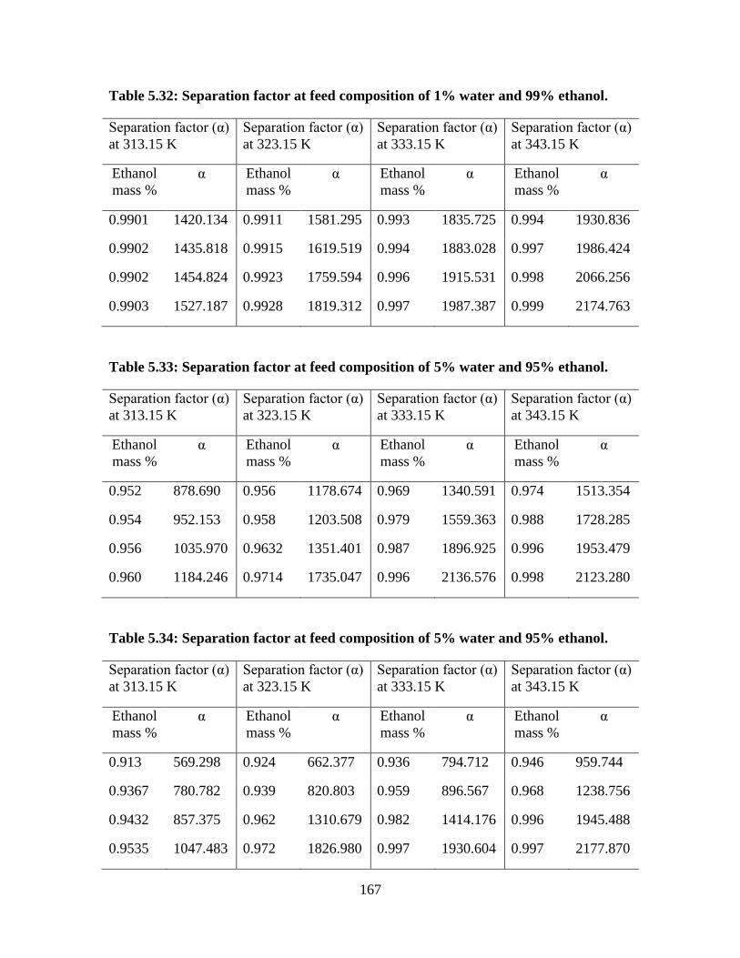
167
Table 5.32: Separation factor at feed composition of 1% water and 99% ethanol.
Separation factor (α)
at 313.15 K
Separation factor (α)
at 323.15 K
Separation factor (α)
at 333.15 K
Separation factor (α)
at 343.15 K
Ethanol
mass %
α Ethanol
mass %
α Ethanol
mass %
α Ethanol
mass %
α
0.9901 1420.134 0.9911 1581.295 0.993 1835.725 0.994 1930.836
0.9902 1435.818 0.9915 1619.519 0.994 1883.028 0.997 1986.424
0.9902 1454.824 0.9923 1759.594 0.996 1915.531 0.998 2066.256
0.9903 1527.187 0.9928 1819.312 0.997 1987.387 0.999 2174.763
Table 5.33: Separation factor at feed composition of 5% water and 95% ethanol.
Separation factor (α)
at 313.15 K
Separation factor (α)
at 323.15 K
Separation factor (α)
at 333.15 K
Separation factor (α)
at 343.15 K
Ethanol
mass %
α Ethanol
mass %
α Ethanol
mass %
α Ethanol
mass %
α
0.952 878.690 0.956 1178.674 0.969 1340.591 0.974 1513.354
0.954 952.153 0.958 1203.508 0.979 1559.363 0.988 1728.285
0.956 1035.970 0.9632 1351.401 0.987 1896.925 0.996 1953.479
0.960 1184.246 0.9714 1735.047 0.996 2136.576 0.998 2123.280
Table 5.34: Separation factor at feed composition of 5% water and 95% ethanol.
Separation factor (α)
at 313.15 K
Separation factor (α)
at 323.15 K
Separation factor (α)
at 333.15 K
Separation factor (α)
at 343.15 K
Ethanol
mass %
α Ethanol
mass %
α Ethanol
mass %
α Ethanol
mass %
α
0.913 569.298 0.924 662.377 0.936 794.712 0.946 959.744
0.9367 780.782 0.939 820.803 0.959 896.567 0.968 1238.756
0.9432 857.375 0.962 1310.679 0.982 1414.176 0.996 1945.488
0.9535 1047.483 0.972 1826.980 0.997 1930.604 0.997 2177.870
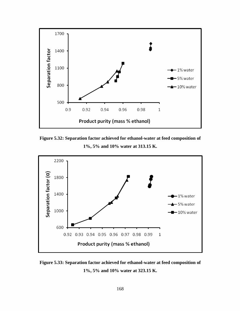
168
Figure 5.32: Separation factor achieved for ethanol-water at feed composition of
1%, 5% and 10% water at 313.15 K.
Figure 5.33: Separation factor achieved for ethanol-water at feed composition of
1%, 5% and 10% water at 323.15 K.
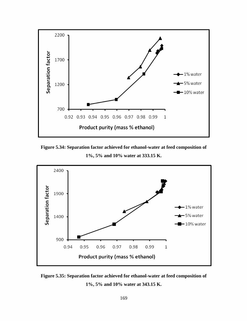
169
Figure 5.34: Separation factor achieved for ethanol-water at feed composition of
1%, 5% and 10% water at 333.15 K.
Figure 5.35: Separation factor achieved for ethanol-water at feed composition of
1%, 5% and 10% water at 343.15 K.
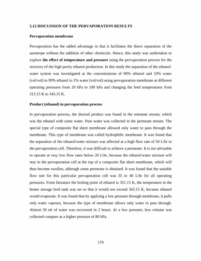
170
5.12 DISCUSSION OF THE PERVAPORATION RESULTS
Pervaporation membrane
Pervaporation has the added advantage in that it facilitates the direct separation of the
azeotrope without the addition of other chemicals. Hence, this study was undertaken to
explore the effect of temperature and pressure using the pervaporation process for the
recovery of the high purity ethanol production. In this study the separation of the ethanol-
water system was investigated at the concentrations of 90% ethanol and 10% water
(vol/vol) to 99% ethanol to 1% water (vol/vol) using pervaporation membrane at different
operating pressures from 20 kPa to 100 kPa and changing the feed temperatures from
313.15 K to 343.15 K.
Product (ethanol) in pervaporation process
In pervaporation process, the desired product was found in the retentate stream, which
was the ethanol with some water. Pure water was collected in the permeate stream. The
special type of composite flat sheet membrane allowed only water to pass through the
membrane. This type of membrane was called hydrophilic membrane. It was found that
the separation of the ethanol/water mixture was affected at a high flow rate of 50 L/hr in
the pervaporation cell. Therefore, it was difficult to achieve a permeate. It is not advisable
to operate at very low flow rates below 20 L/hr, because the ethanol/water mixture will
stay in the pervaporation cell at the top of a composite flat sheet membrane, which will
then become swollen, although some permeate is obtained. It was found that the suitable
flow rate for this particular pervaporation cell was 35 to 40 L/hr for all operating
pressures. From literature the boiling point of ethanol is 351.15 K, the temperature in the
heater storage feed tank was set so that it would not exceed 343.15 K, because ethanol
would evaporate. It was found that by applying a low pressure through membrane, it pulls
only water vapours, because the type of membrane allows only water to pass through.
Almost 50 ml of water was recovered in 2 hours. At a low pressure, less volume was
collected compare at a higher pressure of 80 kPa.
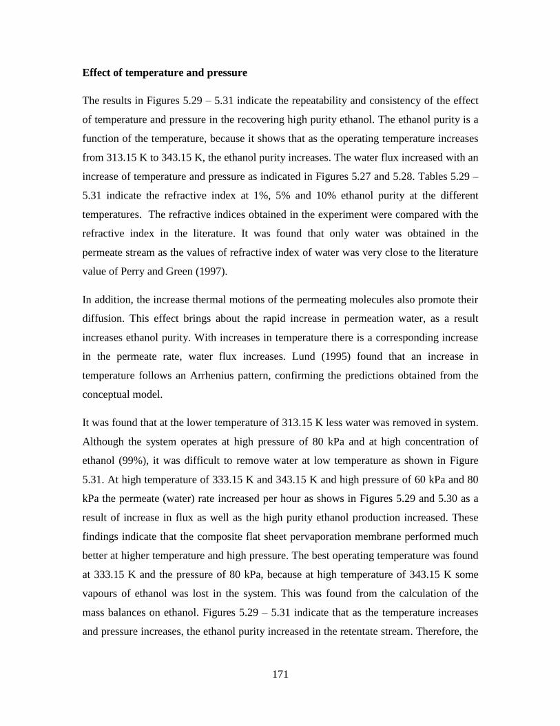
171
Effect of temperature and pressure
The results in Figures 5.29 – 5.31 indicate the repeatability and consistency of the effect
of temperature and pressure in the recovering high purity ethanol. The ethanol purity is a
function of the temperature, because it shows that as the operating temperature increases
from 313.15 K to 343.15 K, the ethanol purity increases. The water flux increased with an
increase of temperature and pressure as indicated in Figures 5.27 and 5.28. Tables 5.29 –
5.31 indicate the refractive index at 1%, 5% and 10% ethanol purity at the different
temperatures. The refractive indices obtained in the experiment were compared with the
refractive index in the literature. It was found that only water was obtained in the
permeate stream as the values of refractive index of water was very close to the literature
value of Perry and Green (1997).
In addition, the increase thermal motions of the permeating molecules also promote their
diffusion. This effect brings about the rapid increase in permeation water, as a result
increases ethanol purity. With increases in temperature there is a corresponding increase
in the permeate rate, water flux increases. Lund (1995) found that an increase in
temperature follows an Arrhenius pattern, confirming the predictions obtained from the
conceptual model.
It was found that at the lower temperature of 313.15 K less water was removed in system.
Although the system operates at high pressure of 80 kPa and at high concentration of
ethanol (99%), it was difficult to remove water at low temperature as shown in Figure
5.31. At high temperature of 333.15 K and 343.15 K and high pressure of 60 kPa and 80
kPa the permeate (water) rate increased per hour as shows in Figures 5.29 and 5.30 as a
result of increase in flux as well as the high purity ethanol production increased. These
findings indicate that the composite flat sheet pervaporation membrane performed much
better at higher temperature and high pressure. The best operating temperature was found
at 333.15 K and the pressure of 80 kPa, because at high temperature of 343.15 K some
vapours of ethanol was lost in the system. This was found from the calculation of the
mass balances on ethanol. Figures 5.29 – 5.31 indicate that as the temperature increases
and pressure increases, the ethanol purity increased in the retentate stream. Therefore, the
172
effect of pressure and temperature increases the performance of the pervaporation using
the hydrophilic membrane.
Figure 5.32 – 5.35 shows the separation factor at 99% ethanol and 1% water (vol/vol),
95% ethanol and 5% water (vol/vol), 90% ethanol and 10% water (vol/vol). The increase
in temperature from 313.15 K to 343.15 K led to the increased of the separation factors.
Results for the separation are tabulated from Tables 5.32 – 5.34. The pervaporation
system operating at low flow rate of 35 l/hr leads to high separation factor but lower flux
as confirmed by Huang et al. (2001).
5.13 Comparison of pervaporation and extractive distillation
When comparing the pervaporation process and extractive distillation, one finds that in
the extractive distillation a third component must be added to the system as a separating
agent, either salt or liquid. In extractive distillation, salt is more effective because it
increases the relative volatility of the ethanol and increases the boiling point of water.
Therefore, calcium chloride salt could be used in the extractive distillation to eliminate
the azeotrope of the ethanol-water system and the high purity ethanol production could be
achieved. These could be achieved using the concentration of 0.3 g/ml of CaCl2 at higher
temperature and pressure. The advantage of extractive distillation using salt is that it does
not need the second column to remove the salt. Alternatively, the pervaporation process
has the advantage of facilitating the direct separation of ethanol-water system as a result
of shifting or eliminating the azeotrope completely from the ethanol-water mixture
without adding the third component as a separating agent. The elimination of the
azeotrope from ethanol-water mixture leads to the recovery of high purity ethanol
production. In addition, pervaporation membrane separation could be considered as one
effective method and energy-saving process for this azeotropic system.
173
CHAPTER 6
CONCLUSIONS AND RECOMMEMDATIONS
6.1 Conclusions
Effect of salt in extractive distillation
A vapour-liquid equilibrium recirculation still was used for the measurement of VLE
data. In this study calcium chloride was chosen because it provides the largest salting out
effect on ethanol. VLE experimentation was performed to assess the ability of calcium
chloride as a separating agent in the extractive distillation. The success of calcium
chloride salt as a separating agent to eliminate or remove the ethanol-water azeotrope,
was achieved at the concentration of 0.2 g/ml and 0.3 g/ml. It shows that at these
concentrations an increase in the relative volatility, results in the recovery of the high
purity ethanol production at the top of the column. The low concentration of 0.1 g/ml did
not eliminate the azeotrope in the ethanol-water system. The interaction parameters were
determined for the excess Gibbs energy models: Wilson and NRTL. The fit of these
models to the experimental data gave low deviations between the calculated and
experimental data. Salt became saturated at the high concentration of 0.4 g/ml.
174
Pervaporation
This study has shown that the composite flat sheet pervaporation membrane could
separate ethanol and water. The increase of water flow rate in the permeate increased the
water flux, as a results of increasing the concentration of the ethanol in the retentate
stream, this leads to the high purity ethanol production. The effects of temperature and
pressure on the pervaporation process increased the performance of the pervaporation
membrane. In additional, pervaporation membrane separation could be considered as one
effective method and energy-saving process for the separation of the azeotropic system.
The pervaporation membrane facilitates the direct separation of ethanol-water system.
6.2 Recommendations
The following recommendations are suggested for use of salt (calcium chloride) in the
extractive distillation process and pervaporation process for the ethanol-water system in
order to achieve high purity ethanol.
Salt in extractive distillation
Further research could be conducted to assess the potential use of the calcium chloride
salt in separation of the ethanol/water system in the extractive distillation above
atmospheric pressure with the concentrations below 0.4 g/ml. It is recommended that
calcium chloride could be recovered at the bottom of the extractive distillation because it
could be used for another purpose. Most researchers presented the experimental VLE data
with no attempt to develop correlations for the binary systems or ternary system. It is
recommended to use the Wilson, NRTL and UNIQUAC models to regress the systems
with salts.
Pervaporation
The pervaporation technique can be considered for commercial applications as it is clear
more investigation need to be done on this particular system as it not applicable for large

175
scale. It is recommended that other processes be employed in the separation of ethanol
and water in the industrial separation. An improvement in developing the mathematical
model is also recommended, as the existing solution procedure involves the fitting of
fluxes. It is suggested to develop a model so that the fluxes and selectivities may be
predicted simultaneously. In addition, it is recommended that the cooling system must be
at least 268.15 K, so that all vapours would condense resulting in more permeate
collected. A hydrophobic membrane could be evaluated with the addition of salt.
176
References
Abbott, M. M., 1986. Low-pressure phase equilibria: Measurement of VLE. Fluid Phase
Equilibria, Vol. 29, (193 – 207)
Abrams, D. S., and Prausnitz, J. M., 1975. Statistical thermodynamics of liquid mixtures:
a new expression for the excess Gibbs energy of partly or completely miscible systems,
American Institute of Chemical Engineers Journal, Vol. 21, p. (116 – 128)
Abu Al-Rub, F. A., Banat, F. A., and Simandl, J., 1999. Isothermal vapour-liquid
equilibria of 1-propanol-water mixtures, Chemical Engineering Journal, Vol. 74, p. (205
– 210)
Anderson, T. F., Prausnitz, J. M., 1978. Application of the UNIQUAC equation to
calculation of multicomponent phase equilibria. 1: VLE; 2. LLE, Industrial and
Engineering Chemistry, Process Design and Development, Vol. 17, p. (552 – 567)
Baker, R. W., 2004. Membrane Technology and Applications, 2nd
Edition, Chichester,
England, Wiley
Belyaev, A. S., Trifonov S. A., and Mushtaev V. I., 2003. Separation of a Propanol-
Water mixture by Membrane Pervaporation, Chemical and Petroleum Engineering, Vol.
39, p. (583 – 587).
Binning, R. C., Lee, R. J., Jennings, J. F., Martin, E. C., 1961. Separation of liquid
mixtures by permeation, Industrial and Engineering Chemistry, Vol. 53, No.1, p. (45 –
50)
Boddeker, K. W., Bengston, G., Pingel, H., 1990. Pervaporation of isomeric butanols,
Journal of Membrane Science, Vol. 54, p. (1 – 12)
Bowen, T. C., Meier, R. G., Vane, L. M., 2007. Stability of MFI zeolite-filled PDMS
membranes during pervaporative ethanol recovery from aqueous mixtures containing
acetic acid, Journal of Membrane Science, Vol. 298, p. (117 – 125)
177
Brubaker, D. W., and Kammermeyer, K., 1954. Separation of gases by plastic
membrane: Permeation rates and extent of separation, Industrial and Engineering
Chemistry, Vol. 46, No.4, p. (733 – 742)
Busca, G., Berardinelli, S., Resini, C., Arriighi, L., 2008. Technologies for the removal of
phenol from fluid streams: A short review of recent development, Journal of Hazardous
Material, Vol. 113, p. (1 – 24)
Calvar, N., Gonzalez, B., Gomez, E., Dominguez, A., 2006. Vapor−liquid equilibria for
the ternary system ethanol + water + 1-butyl-3-methylimidazolium chloride and the
corresponding binary systems at 101.3 kPa, Journal of Chemical Engineering Data, Vol
51, p. (2178 – 2181)
Calvar, N., Gonzalez, B., Gomez, E., Dominguez, A., 2007. Study of the behavior of the
azeotrope ethanol and water with imidazolium based ionic liquids, Fluid Phase
Equilibria, Vol. 259, p. (51 – 56)
Chen, B. H., Lei, Z. G., and Li, J. W., 2003. Effect of salt in the extractive distillation,
Journal Chemical Engineering, Vol. 36, p. (20 – 24)
Chou, T. J., and Tanioka., 1999. Predicting the effect of dissolved salt on the vapour-
liquid equilibria for alcohol-water-salt systems, Trans IChemE, Vol. 77, Part A, p. (329 –
334)
Danner, R. P., and Gess, M. A., 1990. A data base standard for the evaluation of Vapour-
liquid equilibrium models, Fluid Phase Equilibria, Vol. 56, p. (285 – 301)
Dekker, M., 1999. Alcohol/Ether separation by pervaporation. High performance
membrane design, Separation Science and Technology, Vol. 34, No. 3, p. (369 – 390)
Doghier, F., Nardella, A., Sarti, G. C., Valentini, C., 1994. Pervaporation of methanol
MTBE mixtures through modified poly(phenylene oxide) membrane, Journal of
Membrane Science, Vol. 91, p. (283 – 291)
178
Dong, Y. Q., Zhang, L., Shen, J. N., Song, M. Y., Chen, H. L., 2006. Preparation of
poly(vinyl alcohol) sodium algimat hollow-fiber composite membranes and
pervaporation dehydration characterization of aqueous alcohol mixture, Desalination,
Vol. 193, p. (202 – 210)
Driolli, E., 1992. Emerging membrane processes, Recent Progress En Genie Des
Proceeds, Vol. 6, No. 21, p.(339 – 348)
Driolli, E., Zhang, S., and Basile A., 1993. On the coupling effect in pervaporation,
Journal of Membrane Science, Vol. 81, p. (43 – 55)
Duan, Z. T., Lei, L. H., Zhou, R. Q., 1980. Salt effect on vapour-liquid equlibria for
binary systems of propanol/CaCl2 and butanol/CaCl2, Petrochemical Technology
(China), Vol. 9, p. (350 – 353)
Dutta, B. K., and Sikdar, S. K., 1991. Separation of azeotropic organic liquid mixtures by
pervaporation, AICHE, Vol. 37, No. 4, p. (581 – 588)
Fahmi, A., Abu, A-R., Fawzi, A. B., Rami, J., 1999. Vapour-Liquid Equilibrium of
ethanol-water system in the presence of molecular sieves, Separation Science and
Technology, Vol. 34, No. 12, p. (2355 – 2368)
Farve, E., and Vallieres, C., 2004. Pressure versus sweeping gas operation for binary
mixtures separation by dense membrane processes, Journal of Membrane Science, Vol.
244, p. (17 – 23)
Field, R. W., and Lipniziki, F., 2001. Integration of pressure and sweep gas
pervaporation to recover organic compounds from wastewater, Separation and
Purification Technology, Vol. 22 – 23, p. (347 – 360)
Fileti, E. E., Chaudhuri, P., Canuto, S., 2004. Relative strength of hydrogen bond
interaction in alcohol and water complexes, Chemical Physics Letters, Vol. 400, p. (494 -
499)
Fleming, H. L., 1992. Consider membrane pervaporation, Chemical Engineering
Progress, Vol. 5, p. (46 – 52)
179
Fredunslund, A., Gmehling, J., Rasmussen, P., 1977. Vapour-Liquid Equilibrium using
UNIFAC, Elsevier, Amsterdam
Furter, W. F., 1992. Extractive distillation by salt effect, Chemical Engineering
Communication, Vol. 116, p. (35 – 40)
Furter, W. F., 1993. Production of fuel-grade ethanol by extractive distillation employing
the salt effect, Separation and Purification Technology, Vol. 22, No. 1, p. (1 – 21)
Gao, Z., Wang, S., Sun, Q., and Zhang, F., 2003. Isobaric phase equilibria of the system
1-butanol + water containing penicillin G potassium salt at low pressures, Fluid Phase
Equilibria, Vol. 214, p. (137 – 149)
Gess, M. A., Danner, R. P., Nagvekar, M., 1991. Thermodynamics analysis of vapour-
liquid equilibria: Recommended models and a standard data base, Design Institute for
Physical Property Data, American Institute of Chemical Engineers
Gil, I. D., Uyazan, A. M., Aguilar, J. L., Rodriguez, G., Caicedo, L. A., 1996.
Dehydration of azeotrope ethanol by extractive distillation with salt and solvent as an
entrainer, Chemical Engineering Science, Vol. 51, p. (11 – 20)
Gmehling, J and Oken, U., 1977-1982. Vapour-liquid equilibrium data collection,
DECHEMA Chemistry data series, Frankfurt/Main
Gmehling, J., Oken, U., Arlt, W., 1984. Vapour-liquid equilibrium data collection:
Chemistry data series, Vol. 1, Part 8, DECHEMA
Gu, F and Hou, Y., 2000. Salt effects on the Isobaric vapour-liquid equilibrium for four
binary systems, Journal of Chemical Engineering Data, Vol. 45, p. (467 – 470)
Guerreri, G., 1992. Membrane alcohol separation process: Integrated pervaporation and
fractional distillation, Transaction of Institute Chemical Electronics, Part A, Vol. 70, p.
(501 – 508)
180
Haggin, J., 1988. New generation of membranes developed for industrial separations,
Chemical and Engineering News, Vol. 66, p. (7 – 16)
Harris, R. A., 2004. Monoethanolamine: Suitability as an Extraction Solvent, Master of
Science in Engineering (Chemical Engineering) Thesis, University of KwaZulu-Natal,
South Africa
Hayden, J. D., and O'Connell, J. P., 1975. Generalized Method for Predicting Second
Virial Coefficients, Industrial and Engineering Chemistry. Process Design and
Development, Vol.14, p. (209 – 216).
Herington, E. F. G., 1947. A Thermodynamic consistency test for the internal consistency
of experimental data of volatility ratios, Nature, Vol. 160, p. (610 – 611)
Hilal, N., Yousef, G., Anabtawi, M. Z., 2002. Operating parameters effect on methanol-
acetone separation by extractive distillation, Separation Science Technology, Vol. 37, p.
(3291 – 3303)
Hilmen, E.-K., 2000. Separation of Azeotropic Mixtures: Tools for Analysis and Studies
on Batch Distillation Operation, Phd Thesis (Chemical Engineering) University of
Science and Technology, Norwegian
Hirata, M. S., Ohe, S., Nagahama, K., 1975. Computer aided data book of vapour-liquid
equilibria, Kodansha Elsevier, Tokyo
Hollein, M. E., Hammond, M., Slater, C. S., 1993. Concentration of dilute acetone-water
solutions using pervaporation, Separation Science and Technology, Vol. 28, No. 4, p.
(1043 – 1061)
Hoshi, M., Kogure, M., Saitoh, T., Nakagawa, T., 1997. Separation of aqueous phenol
through polyurethane membranes by pervaporation, Journal Applied Polymer Science,
Vol. 65, p. (469 – 479)
181
Howell, D., Coutinho, P., Macedo, E. A., 1989. Infinite-dilution activity coefficients by
comparative ebulliometry. Binary systems containing chloroform and diethylamine, Fluid
Phase Equilibria, Vol. 95 , p. (149 – 162)
Huang, H-J., Ramaswamy, S., Tshirner, U.W., Ramardo, B.V., 2008. A review of
separation technologies in current and future biorefiners, Separation and purification
Technology, Vol 62, p.(1 – 21)
Huang, R. Y. M., 1991. Pervaporation membrane separation processes, Membrane
Science and Technology Series, Elsevier
Huang, R. Y. M., and Jarvis, N. R., 1970.Separation of liquid mixtures by using polymer
membrane II. Permeation of aqueous alcohol solutions through cellophane and poly
(vinyl alcohol), Journal of Applied Polymer Science, vol. 14, p. (2341 – 2356)
Izadifar, M., and Baik, O. D., 2008. An optimum ethanol-water solvent system for
extraction of podophyllotoxin: Experimental study, diffusivity determination and
modeling, Separation and Purification Technology, Vol. 63, No. 1, pp. (53 – 60)
Joseph, A. M., 2001. Computer-aided Measurement of Vapour Liquid Equilibria in a
Dynamic Still at Sub-Atmospheric Pressures, Master of Science in Engineering
(Chemical Engineering) Thesis, University of KwaZulu-Natal, South Africa
Kato, M., Sato, T., Hirata, M., 1971. Measurement of salt effect on vapour-liquid
equilibria by bubble and condensation point method, Journal of Chemical Engineering of
Japan, Vol. 4, p. (308 – 311)
Knight, K. F., Duggal, A., Shelden, R. A., Thompson, E. V., 1986. Dependence of
diffusive permeation rates and selectivities on upstream and downstream pressures, Part
V. Experimental results for the hexane/heptanes (ideal) and toluene/ethanol (non-ideal)
system, Journal of Membrane Science, Vol. 26, p.(31 – 50)
182
Kujawski, W., Pozniak, G., 2004. Swelling properties of ion-exchange membranes in
contact with water-alcohol mixtures, Separation Science and Technology, Vol. 39, p.
(2137 – 3154)
Kumar, A., 1993. Salt effect on vapour-liquid equilibria: A review of correlations and
predictive models, Separation Science and Technology, Vol. 10, No. 10, p. (1799 – 1818)
Kondo, M., and Sato, H., 1994. Treatment of wastewater from phenolic resin process by
pervaporation, Desalination, Vol. 98, p. (147 – 154)
Koops, G. H., and Smolders, C. A., 1991. Estimation and evaluation of polymeric
materials for pervaporation membranes, Elsevier Science Publishers, p. (253 – 278)
Koretsky, D. M., 2003. Engineering and Chemical Thermodynamics, New York, Wiley
Krafczyk, J., Fischer, K, Gmehling. J., Menke, J., 2004. Azeotropic Data, Second,
Completely Revised and Extended Edition, Part 1, Weinheim, Wiley-VCH
Kreiter, R., Wolfs, D. P., Engelen, C. W. R., van Veen, H. M., Vente, J. F., 2008. High-
temperature pervaporation performance of ceramic-supported polyimide membranes in
the dehydration of alcohols, Journal of Membrane Science, Vol. 29, p.(13 – 20)
Letcher, T. M., 2004. Chemical Thermodynamics for Industry, Cambridge, Royal Society
of Chemistry
Lee, L-S., and Huang, M-Y., 2000. The vapour-liquid equilibrium of ethanol-water
mixture in the presence of benzyltriethylammonium chloride salt at atmospheric pressure,
Chemical Engineering Communication, Vol. 180, No. 1, p. (19 – 38)
Lee, K-R., Liu, M-J., Lai, J-Y., 1994. Pervaporation separation of aqueous alcohol
solution through asymmetric polycarbonate membrane, Separation Science and
Technology, Vol. 29. No. 1, p. (119 – 134)
Lei, Z., Wang, H., Zhou, R., Duan, Z., 2002. Solvent improvement for separating C4 with
ACN , Separation Science and Technology, Vol 26, p. (1213 – 1221)
183
Lei, Z., Wang, H., Zhou, R., Duan, Z., 2002.Influence of salt added to solvent on
extractive distillation, Chemical Engineering Journal, Vol. 87, p. (149 – 156)
Lei, Z., Li, C., Chen, B., 2003. Extractive distillation: A review, Separation and
Purification reviews, Vol. 32, No. 2, p. (121 – 213)
Lightning Africa, May 2005. Chemical Technology, Features: Design and Construction of
Chemical Plant, Water treatment, Material and Chemical product design and Solids
Handling
Lipnizik, F., Field, R. W., 2001. Integration of pressure and sweep gas pervaporation to
recover organic compounds from wastewater, Separation and Purification technology,
Vol. 22-23, p. (347 – 360)
Liu, X., Sun, Y., Deng, X., 2008. Studies on the pervaporation membrane of permeation
water from methanol/water mixture, Journal of membrane Science, Vol. 325, p. (192 –
198)
Loeb, Y. C., 1958. Study of the asymmetric pervaporation membrane, Journal of
Membrane Science, Vol. 343, p. (176 – 179)
Lund, J. G., 1995. Pervaporative separation of oleinic/oxygenate hydrocarbon mixtures,
Master of Science in Engineering (Chemical Engineering) Thesis, University of
KwaZulu-Natal, South Africa
Ma, Y., Wang, J., Tsuru, T., 2009. Pervaporation of water/ethanol mixtures through
microporous silica membranes, Separation and Purification Technology, Vol. 42, p. (33 –
39)
Malanowski, S., Anderko, A., 1992. Modelling phase equilibria – Thermodynamic
background and practical tools, Wiley Series in Chemical Engineering, John Wiley &
Sons, New York, Chichester,
Malasinksi, W., 1965. Azeotropy and other theoretical problems of vapour-liquid
equilibrium, Interscience, New York
184
Mariah, L., 2006. Membrane distillation of concentrated brines, Phd Thesis (Chemical
Engineering), University of KwaZulu-Natal, South Africa
Mario, L-R., and Jamie, A-A., 2003. Modeling and simulation of saline extractive
distillation columns for the production of absolute ethanol, Computer & Chemical
Engineering, Vol. 27, Issue 12, p. (527 – 549)
Marsh, K. N., 1989. New methods for vapor-liquid-equilibria measurements, Fluid Phase
Equilibria, Vol. 52, p. (169 – 184)
Marquardt, D. W., 1963. An algorithm for least-squares estimation of non-linear
parameters, Journal. Society of Industrial and Applied Mathematics, Vol. 11, p. (431 –
441)
Marzal, P., Monton, J. B., Rodrigo, A., 1996. Isobaric vapour –liquid equilibria of the
water + 2-propanol system at 30, 60 and 100 kPa, Journal of Chemical Engineering
Data, Vol. 41, p. (608 – 611)
McCandless, F. P., Alzheimer, D. P., Hartman, R. B., 1974. Solvent membrane
separation of benzene and cyclohexane, Process Design and development, Vol. 12, No. 3,
p. (310 – 312)
Mohammad, S., and Taghi, Z-A., 1996. A modified solution-diffusion model for
separation of ethanol-water azeotrope mixtures in pervaporation, Chemical Engineering
Communication, Vol.152, p. (405 – 412)
Mulder, M. H. V., Franken, T., Smolders, C. A., 1985. Preferential sorption versus
preferential permeability in pervaporation, Journal of Membrane Science, Vol. 22, p.
(155 – 173)
Nakane, T., and Yanagishita, H., 1992. Preparation of asymmetric polyimide membranes
by the phase inversion process, Koubunshi Ronbunshu, Vol. 49, p. (1015 – 1021)
185
Namboodiri, V. V., Bowen, T. C., Vane, L. M., 2006. Selective of Ethanol from water by
pervaporation: Zeolite-silicone rubber mixed matrix membranes, Separation and
Purification Technology, Vol. 125, p. (305-308)
Narasigadu, C., 2006. Phase equilibrium investigation of the water and acetonitrile
solvent with heavy hydrocarbons, Master of Science in Engineering (Chemical
Engineering) Thesis, University of KwaZulu-Natal, South Africa
Neel, J., 1991. Introduction to pervaporation, In: “Pervaporation membrane separation
processes” Elsevier Science Publishers, p. (1 – 109)
Nomura, M., Bin, T., Nakao, S. I., 2002. Selective ethanol extraction from fermentation
broth using a silicate membrane, Separation Science and Technology, Vol. 27, p. (59 –
66)
O‟Brien, D. J. and Craig, J. C., 1996. Ethanol production in a continuous
fermentation/membrane pervaporation system, Applied Microbiology Biotechnology,
Vol. 44, p. (699 – 704)
Ohe, S., 1979. Correlation and prediction of salt effects on vapor–liquid equilibrium in
alcohol–water–salt systems, Advances in Chemistry Series, No. 155
Ohe, S., 1991. Computer Aided Data book of vapour pressure (Liquid-Vapour
Equilibrium in Binary Systems), Tokyo, Kodansha
Ohe, S., 1998. Prediction of salt effect on vapour-liquid equilibria, Fluid Phase
Equilibria, Vol. 144, p. (119 – 129)
Ophardt, P., 2003. Chemistry of hydrogen bond, Journal of Applied Chemisrty, Vol. 73,
p. (18 – 24)
Orye, R. V., and Prausnitz, J. M., 1965. Multicomponent equilibria with the Wilson
equation, Industrial and Engineering Chemistry, Vol. 57, p. (18 – 26)
Palmer, D. A., 2000. Handbook of Applied Thermodynamics, 2nd
Edition, McGraw-Hill.
186
Parke, S. A., and Birch, G. G., 1999. Solution properties of ethanol in water, Food
Chemistry, Vol. 67, p. (241 – 246)
Paulsen, V. S., 2002. Use a spreadsheet to fit vapour-liquid equilibrium data, Chemical
Engineering, No. 3, p. (78 – 81)
Peinemann, K. V. and Nunes, S. P., 2001. Membrane Technology in the chemical
industry, Weinheim, New York, Wiley-VCH
Pereiro, A. B., Rodriguez, A., 2007. Mixing properties of binary mixture presenting
azeotropes at several temperatures, Chemical Engineering Journal, Vol 39, p. (1219 –
1230)
Peng, M., Vane, L. M., Liu, S. X., 2003. Recent advances in VOCs removal from water
by pervaporation, Journal of Hazardous Material, B98 p. (69 – 90)
Perry, R. H., and Green, D. W., 2004. Perry’s Chemical Engineers Handbook, McGraw
Hill Handbook, New York
Pitzer, K. S., and Curl., R. F., 1957. Emperical Equation for the Second Virial
Coefficient, Journal of the American Chemical Society, Vol. 79, p. (2369 – 2370).
Pitzer, K. S., Lippmann, D. Z., Curl, R. F., Huggins, C. M., Petersen, D. E., 1955, The
Volumetric and Thermodynamic Properties of Fluids. II. Compressibility Factor, Vapour
Pressure and Entropy of Vapourization, Journal of the American Chemical Society, Vol.
77, p. (3433 – 3440)
Prausnitz, J. M., Lichtenthaler, R. N., de Azevedo, E. G., 1978. Molecular
Thermodynamics of Fluid – Phase Equilibria, 3rd
Edition, Prentice-Hall, Upper Saddle
River, New Jersey
Prausnitz, J. M., Lichtenthaler, R. N .,and de Azevedo, E. G., 1999. Molecular
Thermodynamics of Fluid-Phase Equilibria, 3rd
Edition, Prentice-Hall, Upper Saddle
River, New Jersey
187
Poling, B. E., Prausnitz, J. M., O‟Connel, J. P., 2001. The Properties of Gas and Liquids,
5th
Edition, McGraw-Hill
Raal, J. D., Mühlbauer A. L., 1998. Phase Equilibria: Measurement and Computation,
Taylor & Francis, Briston PA
Raghunath, B., Hwang, S. T., 1992. Effect of boundary layer mass transfer resistance in
the pervaporation of dilute organics, Journal of Membrane Science, Vol. 65, p. (147 –
161)
Rakshit, S. K., Ghosh, P., Bisaria, V. S., 1993. Ethanol separation by selective
adsorption of water, Bioprocess Engineering,Vol. 8, pp. (279 – 282)
Rath, P., Naik, S. C., 2004. Prediction of salt effect in vapour-liquid equilibria of system
ethyl acetate-ethanol at atmospheric pressure, Vol. 84, p. (71 – 76)
Rautenbach, R., Albrecht, R., 1980. Separation of organic binary mixtures by
pervaporation, Journal of Membrane Science, Vol. 7, p. (203 – 223)
Rautenbach, R., Albrecht, R., 1984. On the behavior of asymmetric membranes in
pervaporation, Journal of Membrane Science, Vol. 19, p. (1 – 22)
Rautenbach, R., Herion, C., Franke, M., Asfour, A-F. A., Bemquerer-Costa, A., 1988.
Investigation of mass transport in asymmetric pervaporation membranes, Journal of
Membrane Science, Vol. 36, p. (445 – 462)
Reddy, P., 2006. Development of a novel apparatus for VLE measurement at moderate
pressures, Phd Thesis (Chemical Engineering) University of KwaZulu-Natal, South
Africa
Redlich, O., Kister, A. T., 1948. Algebraic Representation of Thermodynamic Properties
and the Classification of Solutions, Industrial and Engineering Chemistry, Vol. 40, p.
(345 – 348)
188
Redman, J., 1990. Pervaporation heading for new horizons, Chemical Engineer, Vol.
469, p. (46 – 49)
Renon, H., and Prausnitz, J. M., 1968. Local Compositions in Thermodynamic Excess
Functions for Liquid Mixtures, American Institute of Chemical Engineers Journal, Vol.
14, p. (135 – 144)
Roizard, D., Jonquieres, A., Leger, C., Noezar, I., and Nee, J., 1999. Alcohol/Ether
Separation by pervaporation: High Performance Membrane Design, Separation Science
and Technology, Vol. 34, No. 3, p. (369 – 390)
Rongqi, Z., and Zhanting, D., 1998. Extractive Distillation with salt in solvent, Journal of
Chemical Engineering of Japan, Vol. 22, p. (1 – 6)
Sada, E., Morisue, T., and Yamaji, H., 1975. Salt effect on isobaric vapour-liquid
equilibrium of isopropanol-water system, The Canadian of Chemical Engineering, Vol.
53, p. (350 – 353)
Sandler, S.I., 1999. Chemical and Engineering Thermodynamics, third ed., John Wiley
and Sons, New York
Seiler, M., Jork, C., Kavarnon, A., Arlt, W., Hiresh, R., 2001. Separation azeotorpic
mixtures using ionic liquids, AIChE Journal, Vol. 50, No. 10, p. (2439 – 2454)
Sevgili, L. M and Senol, A., 2006. Isobaric (vapour + liquid) equilibrium for (2-
propanol + water + ammonium thiocyanate): Fitting the data by an empirical, Journal
Chemical Thermodynamics, Vol. 38, p. (1539 – 1545)
Shao, P., and Huang, R.Y.M., 2006. Review of polymeric membrane pervaporation,
Journal of Membrane Science, Vol. 143, P. (1 – 18)
Slusher, J. T., Decker, K. J., Liu, H., Vega, C. A., Cummings, P. T., O‟Connell, J. P.,
1994. Vapour-liquid equilibria and salt apparent molar volumes of the water + 2-
189
propanol + tetrabutylammonium bromide system, Journal of Chemical Engineering Data,
Vol. 39, p. (506 – 509)
Smith, R., 1995. Chemical Process Design, McGraw-Hill, Inc
Smith, J. M., Van Ness, H. C., Abbott, M. M., 2001. Introduction to Chemical
Engineering Thermodynamics, Sixth Edition, McGraw-Hill International Edition
Sommer, S., Melin, T., 2000. Zeolite membranes in chemical industry, in the 2000 18th
Annual Membrane Technology/Separation Planning Conference, Boston, Massachusetts,
USA.
Sun, R. Y., 1999. Molecular thermodynamics of salt effect in vapour-liquid equilibrium
of ethanol-water system, Fluid Phase Equilibria, Vol. 157, p. (29 – 40)
Sun, T., Bullock, K. R., and Teja, A. S., 2004. Correlation and prediction of salt effects
on vapour-liquid equilibrium in alcohol-salt-salt systems, Fluid Phase Equilibria, Vol.
219, p. (257 – 264)
Swietoslawski, W., 1963. Azeotropy and polyazeotropy, Oxford Pergamon Press
Tan, T. C., 1987. Model for predicting the effect of dissolved salt on the vapour liquid
equilibrium of solvent mixtures, Chemical Engineering Residence Desilation, Vol. 65, p.
(355 – 367)
Tarakad, R. R., Danner, R. P., 1977. An improved corresponding states method for polar
fluids: Correlations of Second Virial Coefficients, American Institute of Chemical
Engineers Journal, Vol. 23, p. (685 – 695)
Teplyakov, V.,1991. Membrane gas separation in petrochemistry: Problem of the
polymeric membrane selection, In: “Effective Industrial membrane Processes: Benefits
and Opportunities” Elsevier Science Publishers, p. (401 – 415)
Teng, M-Y., Lee, K-R., Liaw, D-J., Lai, J-Y., 2000. Preparation and pervaporation
performance of poly(3-alkylthiophene) membrane, Polymer, Vol. 41, p. (2047 – 2052)
190
Thoma, S., Resch, A., Voelz., 1998. Pervaporation: Case Study, p. (1 – 11)
Thongsukmak, A., Sirkar, K. K., 2008. Extractive pervaporation to separate ethanol
from its dilute aqueous solutions characteristics of ethanol-producing fermentation
processes, Journal of Membrane Science, Vol. 28, p. (1 – 44)
Tsonopoulos, C., 1974. An Emperical Correlation of Second Virial Coefficients,
American Institute of Chemical Engineers Journal, Vol. 20, p. (263 – 272)
Tsuboka, T., Katayama, T., 1975. Modified Wilson Equation for Vapour-Liquid and
Liquid-Liquid Equilibria, Journal of Chemical Engineering of Japan, Vol. 8, p. (181 –
187)
Vane, L. M., 2005a. Pervaporation-Membrane process for bioethanol recovery, solvent
dehydration and contaminant removal, Case study, p. (1 – 5)
Vane, L. M., 2005b. A review of pervaporation for product recovery from recovery from
biomass fermentation processes, Journal Chemical Technology. Biotechnology, Vol. 80,
p. (603 – 629)
Van Ness, H. C., 1959. Exact forms of the coexistence equation for binary vapour-liquid
equilibrium, American Institute of Chemical Engineers. Journal, Vol. 16, p. (18 – 22)
Van Ness, H. C., 1995. Thermodynamics in the treatment of vapour/liquid equilibrium
(VLE) data, Pure and Applied Chemistry, Vol. 67, p. (859 – 872)
Van Ness, H. C., Abbott, M. M, 1982. Classical Thermodynamics of nonelectrolyte
solutions: With Applications to Phase Equilibria, McGraw-Hill, New York.
Van Ness, H. C., Byer, S. M., Gibbs, R. E., 1973. Vapour-liquid equilibrium: Part I. An
appraisal of data reduction methods, American Institute of Chemical Engineers Journal,
Vol. 19, p. (238 – 244)
191
Verhoef, A., Figoli, A., Leen, B., Bettens, B., Drioli, E., Van der Bruggen, B., 2008.
Perfomance of a nanofiltration membrane for removal of ethanol from aqueous solutions
by pervapoaration, Separation and Purification Technology, Vol. 60, p. (54 – 63)
Volkov, V. V., 1994. Reviews separation of liquids by pervaporation through polymeric
membranes, Russian Chemical Bulletin, Vol. 43, No. 2, p. (208 – 219)
Walas, S. M., 1985. Phase Equilibrium in Chemical Engineering, Butterworth, Boston
Wang, X-P., Feng, Y-F., Shen, Z-Q., 2000. Pervaporation properties of a three-layer
structure composite membrane, Journal of Applied Polymer Science, Vol. 75, No. 6, p.
(740 – 745)
Wang, L., Li, J., Lin, Y., Chen, C 2007. Separation of dimethyl carbonate/methanol
mixtures by pervaporation with poly(acrylic acid)/poly (vinyl alcohol) blend membranes,
Journal of Membrane Science, Vol. 305, p. (283 – 246)
Watson, J. M., and Payne, P. A., 1990. A study of organic compound pervaporation
through silicone rubber, Journal of Membrane Science, Vol. 49, p. (171 – 205)
Weast, R. C., 1983-1984. CRC Handbook of chemistry and physics, CRC Press
Wesslein, M., Heintz, A., Lichtenthaler, R. N., 1990. Pervaporation of liquid mixtures
through poly (vinyl alcohol) (PVA) membranes II. The binary systems methanol/1-
propanol and methanol/dioxane and the ternary system water/methanol/1-propanol,
Journal of Membrane Science, Vol. 51, p. (181 – 188)
Wessling, M., Werner U., Hwang, S-T., 1991. Pervaporation of aromatic C8- isomers,
Journal of Membrane Science, Vol. 57, p. (257 – 270)
Wilson, G. M., 1964. Vapour-Liquid Equilibrium. XI: A New Expression for the Excess
Free Energy of Mixing, Journal of the American Chemical Society, Vol. 86, p. (127 –
130)
192
Wisniak, J., Tamir, A., 1978. Mixing and excess thermodynamic properties. A literature
source book, Elsevier Scientific Publishing Company, Amsterdam
Xu, y., Chen, C., Zhang, P., Sun, B., Li, J., 2006. Pervaporation properties of polyimide
membranes for separation of ethanol + water mixtures, Journal of Chemical Engineering
data, Vol. 51, p. (1841 – 1845)
Yampolskii, Y. P., Volkov, V. V., 1991. Studies in gas permeability and membrane gas
separation in the Soviet Union, Journal of Membrane Science, Vol. 64, p. (191 – 228)
Yuzhong, Z., Keda, Z., Jiping, X., 1993. Preferential sorption of modified PVA
membrane in pervaporation, Journal of Membrane Science, Vol. 80, p. (297 – 308)
Zhigang, L., Biaohua, C., Zhongwei, D., 2005. Special distillation process, British
Library, ELSEVIER
Zhigang, L., Chengyne, L., Biashua, C., 2003. Extractive distillation: A review,
Separation and Purification reviews, Vol. 32, No. 2, p. (121 – 213)
Zhigang, L., Hongyou, W., Rongqi, Z., Zhanting, D., 2002.Influence of salt added to
solvent on extractive distillation, Chemical Engineering Journal, Vol. 87, p. (149 – 156)

193
Appendix A
LOW PRESSURE VLE CALCULATION METHODS
Ideal system or ideal solution
The assumption of ideal systems i.e. ideal gas and ideal solution provide useful models
that serve as a standard to which real systems can be compared. Ideal solution is a
solution that obeys Raoult‟s law. An ideal gas is a model gas comprising imaginary
molecules of zero volume that were not interact. Consider at a low pressure (pressure
below 1 bar) all the intermolecular forces are approximately the same. Treat the vapour as
an ideal gas and liquid as an ideal solution. The fugacity coefficient in the liquid phase is
approximately equal to the fugacity coefficient in the vapour phase, from the
Lewis/Randall reference state;
i i
o (A.1)
and as the vapour is treated as ideal the Poynting factor exp1
RTv dPi
l
is
approximately unity at lower pressure and the equation can be simplified as:
y P x fi i i (A.2)
Applying equation for the pure species fugacity, it becomes:
y P x Pi i i
sat (A.3)
this equation is known as Raoult‟s law
Non ideal system or liquids
Real system follow Raoult‟s law, if there is form of chemical interaction between the
component a and b (e.g., a-ethanol and b-water). Since it unlikely that a-a interaction is
identical to the a-b interaction. Consider the behavior of some real binary systems for low
pressure for the vapour phase to be ideal gas. The case where the like (a-a and b-b)
194
interaction is stronger than the unlike (a-d) interaction ( i > 1) as well as when the like
interaction is weaker ( i < 1). If the vapour phase is non ideal then use fugacity
coefficient and if the liquid phase is nonideal then use activity coefficient. The following
equation applies:
y P x fi i
v
i i
l
i
o (A.4)
and, from the Lewis/Randall reference state;
f fi
o
i (A.5)
Assume that the vapour phase can be represented as an ideal gas and the fugacity of the
pure liquid is given by Pi
sat . Therefore, the VLE behavior for weakly associating systems
can be described with the required accuracy by the following simplified equation:
x P y Pi i i
sat
i (A.6)
The vapour pressure of pure component i at the system is calculated from Antoine
equation which is:
)()(log
0 CTC
BAkPaP sat
(A.7)
The binary system that has low volatile is known as azeotropic mixture and the
composition are reversible. Azeotropic occurs where the composition of vapour and
liquid are equal. The relationship for the partition coefficient, Kj or VLE ratio is defined
by: Ky
x
P
Pi
i
i
i i
sat
(A.8)
The separation factor or the ratio of the K-value of two species is called the relative
volatility, ij . It can be derived by:
ij
i
j
i i
sat
j j
sat
K
K
P
P (A.9)
195
In the case of azeotropic system, no separation of ethanol/water could be achieved
therefore ij 1. The systems where the difference ij 1 the separation factor is close
to unity, then a large number of theoretical stages are required and a special distillation
process has to be used.
Liquid mixture
For liquid mixture in equilibrium with its vapour, the following three conditions must be
met:
The temperature of liquid and vapour must be equal for there to be thermal
equilibrium
The pressure must be equal for there to be mechanical equilibrium.
The Gibbs free energy must be at a minimum with respect to a transfer of any
component from liquid to gas or gas to liquid.
Phase rule
The conditions for there to be equilibrium between two or more phases are the pressure P,
the temperature T, and chemical potential or fugacity of each substance i shall have the
same value in every phase or the intensive state of PVT system is established when its
temperature, pressure and the compositions of all phases are fixed. However, for
equilibrium state these variables are not all independent and fixing a limited number of
them automatically establishes the others. This number of independent variable is given
by phase rule and its called the number of degrees of freedom of the system. It is the
number of variable which may be arbitrarily specified and which must be specified in
order to fix the intensive state of a system at equilibrium. This number is the difference
between the number of variables needed to characterize the system and the number of
equations that may be written connecting these variables. For a system containing N
chemical species distributed at equilibrium among phases. The phase rule variable are
temperature, pressure, presumed uniform throughtout the system and N – 1 mole
fractions in each phase. The number of these variables is 2 + (N – 1) . The masses of the
196
phase are not phase rule variable because they have nothing to do with the intensive state
of the system. The Duhem‟s theorem is another rule similar to the phase rule, but less
celebrated. It applies to closed systems at equilibrium for which the extensive state as
well as the intensive state of the system is fixed. Duhem‟s theorem is stated as follows:
for any closed system formed initially from given masses of prescribed chemical species,
the equilibrium state is completely determined when any two independent variables are
fixed. The equations that may be written connecting the phase rule variables are:
iii ....... (A.10)
for each species, i giving ( ) 1 N phase equilibrium state
i ii
dn 0 (A.11)
for each independent chemical reaction, giving r equations. The total number if
independent equations are therefore ( ) 1 N r . In their fundamental forms these
equations relate chemical potentials which are functions of temperature, pressure and
composition of the phase rule variable. Since the degree of freedom of the system, F is
the difference between the number of variable and the number of equations:
F N N r 2 1 1( ) ( ) (A.12)
or
F N r 2 (A.13)
The number of independent chemical reactions r can be determined as follows:
Write formation reactions from the elements for each chemical compound present in
the system.
Combine these reaction equations so as to eliminate from the set all elements not
present as elements in the system.

197
The Phase Equilibrium Computation
The fundamental principles of phase equilibrium so far discussed can be applied in some
important VLE calculations. These can be applied to both ideal and nonideal chemical
system involving binary or multi-component mixture. The basic equation for VLE:
f
PP y Px
i
i i i i
. . (A.14)
These are applicable to in all case.
Ideal system
Ideal systems have both fugacity and activity coefficient equal to unity or equal to
1,f
Pi
i
1. The general expression for VLE simplifies down to: Pyi = Pixi, this is
known as Raoult‟s Law. This relationship is used in the calculation of bubble point and
dew point.
The Bubble Point Calculations
Bubble point calculations were performed when the liquid phase composition (all the
xi‟s) is known and the vapour composition (the yi‟s) are required to calculate as well as
bubble point temperature or pressure. The steps in the trial and error procedure are as
follows according to Smith and Van Ness (1987). There are two types of bubble point
calculations
Bubble point temperature calculations: when the liquid composition and system
pressure (P) are known.
The bubble point pressure calculations: when the liquid composition and system
temperature (T) are known
The bubble point temperature calculations: for an ideal system of known liquid
composition (the xi‟s) and at given pressure, P, the bubble point temperature (TB) can be
determined graphically from T-x-y diagram (TB is read off the T vs x curve at the
specified P) or analytically by using the equation: Pyi = Pixi
198
Rearranging equation to: yP
Pxi
i
i
(A.15)
Since the sum of the Pisat
entire component in the vapour phase is unity or equal to 1.
N
i
i
iN
i
i xP
Py
11
1 (A.16)
where: N = number of components
P = pressure being constant
N
i
ii xPP1
(A.17)
This equation has only one unknown parameter and that one is the temperature – since
the vapour pressure of pure component are functions only of temperatures (T). These
equations equation can be solved analytically for T provided and the Antoine type
expression correlating vapour pressure with temperature.
The routine calculation follows the steps outlined belows by Smith et al. (2001):
Assume a suitable temperature (T).
Calculate the vapour pressure Pi of each component at the assumed temperature (T) or
look up at the vapour pressure vs temperature plot to find the Pj of each component.
Calculate the total pressure: P Pxcal
i ii
NC
1
which depends only on temperature.
Check whether the calculated value of total pressure (Pcal
) is sufficiently close to the
actual system pressure. If the margin is small enough then assume another temperature
is the acceptable. If Pcal
is greater than P, then a second set of approximation (with
lower value of T) is required and the procedure is to repeat.

199
The Dew Point Calculations
The dew point temperature calculations: when the vapour composition (the yi‟s) and
system pressure (P) are known.
The dew point pressure calculations: when the vapour composition (the yi‟s) and
system temperature (T) are known
Both calculations are based on the equation: xP
Pyi
i
i
. Since sum of all mole fraction
term is liquid phase is unity or equal to 1.
N
i i
i
i
N
i i
N
i
iP
yPy
P
Px
111
1 (A.18)
Therefore
N
i i
i
P
yP
1
1 (A.19)
This equation has only one unknown variable and that one is either pressure (if the
system temperature is given) or temperature (if the system pressure is given). Dew point
temperature calculations: this is to be done by trail and error method converging on the
correct temperature. The system pressure, P, is given and all the yj‟s are known.
The working procedure follows
Assume a suitable temperature value of temperature.
Determine the vapour pressure of the components at this temperature.
Put these vapour pressure data in the
N
i i
i
P
yP
1
1 to calculate the total pressure, P
cal
Check whether Pcal
is sufficient close to P. if the Pcal
is too far from P, switch over to
second set of approximation, assume T again and repeat the process all over again.
200
Nonideal System
The equation: Pyi = Pixi does not work well for nonideal systems, as they do not obey
Raoult‟s Law. The equation f
PP y Px
i
i i i i
. . can still be use for bubble point and dew
point calculations, provided the activity coefficients are available.
Bubble Point Calculations
The above equation can be rearranged to: yf
P
P
Pxi
i
i
i i
. Assuming the gas phase
behavior is close to ideality | f/P|j = 1 and hence the equation becomes yx P
Pi
i i
i
. The
values of activity coefficient of individual components must be available. The working
procedure for bubble point calculation for nonideal system is similar to that used in the
ideal case.
Since
N
i
N
i
i
ii
iP
Pxandy
1 1
1,1 (A.20)
Therefore
N
i
iii xPP1
(A.21)
The working procedure follows
Assume a suitable temperature (T).
Calculate the vapour pressure Pi of each component at the assumed temperature (T)
from Antoine type equation or look up at the vapour pressure vs temperature plot.
Calculate the total pressure:
N
i
iii
calc xPP1
(A.22)
Check whether the calculated value of total pressure (Pcal
) is sufficiently close to the
actual system pressure. If not, then assume another temperature unit converged.
201
If K – values are used the bubble point calculation can be made on basis of following
equation: yi = Kixi
Therefore:
N
i
ii
N
i
i xKy11
1 (A.23)
Where Ki = distribution coefficient for component i
It is function of temperature, pressure and compositions
Working Procedure as follows
Assume a suitable temperature (T).
Determine the K – values of all component (De Priest chart)
Check whether the
N
i
ii xK1
1 . If sum of Kixi term is unity or 1, the correct
temperature has been assumed, if not repeat the procedure by assuming another
temperature.
The Dew Point Calculations
The dew point calculation is more difficult than bubble point calculations. It is requires
the process of iteration to determine the activity coefficient for the components as much
as the liquid compositions of the components are known.
The working procedure follows
Assume a suitable temperature (T).
Calculate the vapour pressure Pi of each component at the assumed temperature (T)
from Antoine type equation or look up at the vapour pressure vs temperature plot.
Determines the xi‟s
Use the valves of xi through the process of iteration to calculate new activity
coefficients
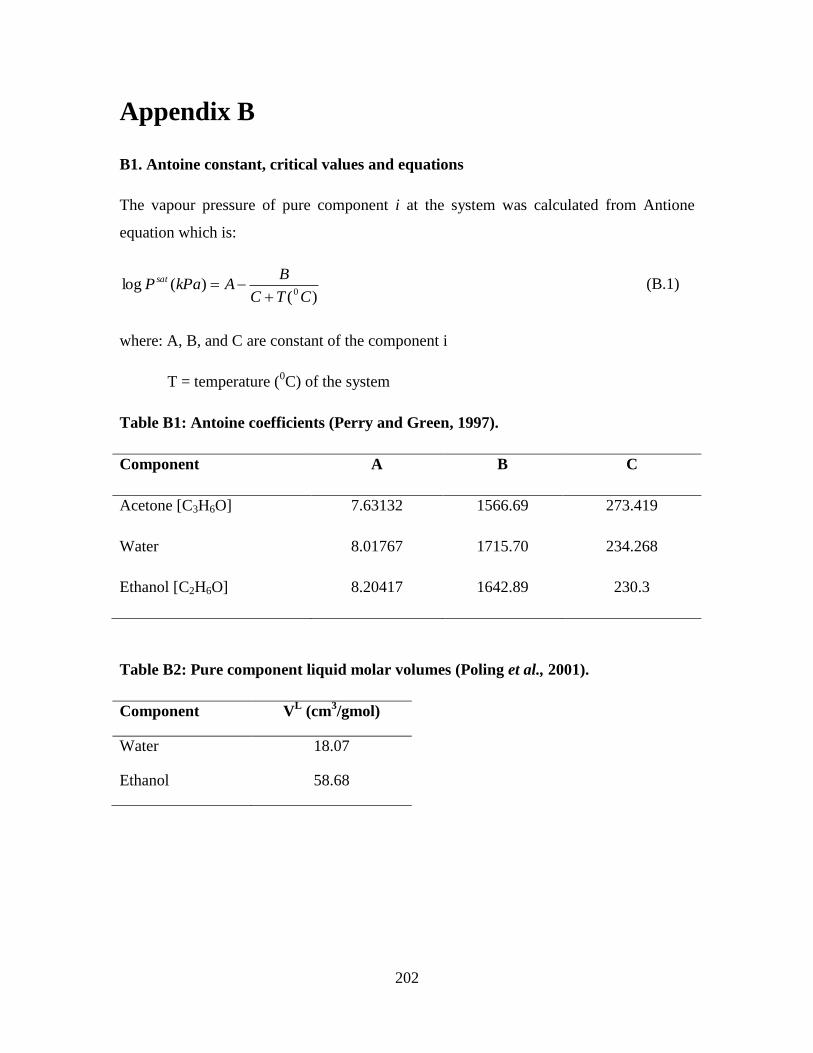
202
Appendix B
B1. Antoine constant, critical values and equations
The vapour pressure of pure component i at the system was calculated from Antione
equation which is:
)()(log
0 CTC
BAkPaP sat
(B.1)
where: A, B, and C are constant of the component i
T = temperature (0C) of the system
Table B1: Antoine coefficients (Perry and Green, 1997).
Component A B C
Acetone [C3H6O] 7.63132 1566.69 273.419
Water 8.01767 1715.70 234.268
Ethanol [C2H6O] 8.20417 1642.89 230.3
Table B2: Pure component liquid molar volumes (Poling et al., 2001).
Component VL (cm
3/gmol)
Water 18.07
Ethanol 58.68

203
Table B3: Critical values and acentric factors for selected component (Poling et al.,
2001).
Component Tc (K) Pc (kPa) Vc (cm3/gmol) zc ω
Water 647.3 22120 57.1 0.235 0.344
Ethanol 513.9 6140 167.1 0.240 0.644
Where: Ji = is the permeation flux through the membrane
L = is the membrane thickness
Pi
G = is the separation permeability coefficient.
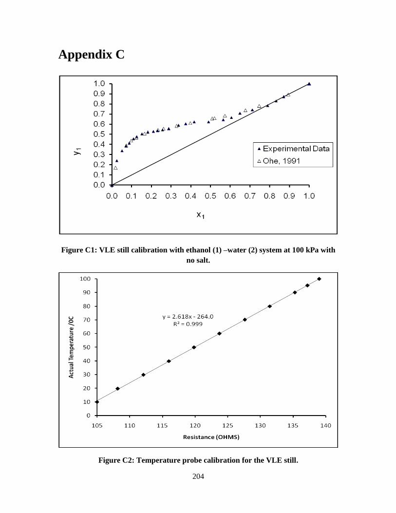
204
Appendix C
Figure C1: VLE still calibration with ethanol (1) –water (2) system at 100 kPa with
no salt.
Figure C2: Temperature probe calibration for the VLE still.
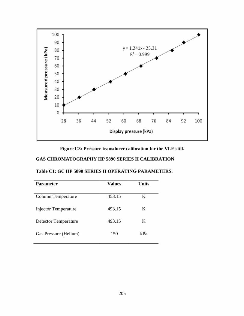
205
Figure C3: Pressure transducer calibration for the VLE still.
GAS CHROMATOGRAPHY HP 5890 SERIES II CALIBRATION
Table C1: GC HP 5890 SERIES II OPERATING PARAMETERS.
Parameter Values Units
Column Temperature 453.15 K
Injector Temperature 493.15 K
Detector Temperature 493.15 K
Gas Pressure (Helium) 150 kPa
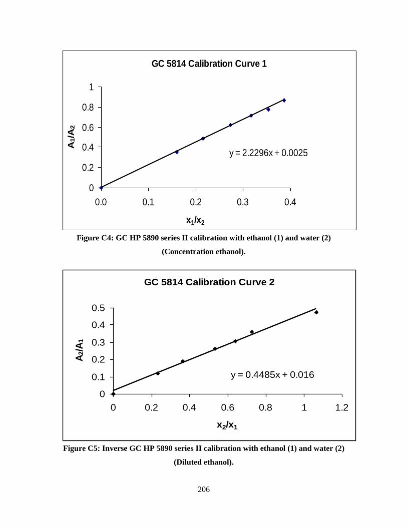
206
GC 5814 Calibration Curve 1
y = 2.2296x + 0.0025
0
0.2
0.4
0.6
0.8
1
0.0 0.1 0.2 0.3 0.4
x1/x2
A1/A
2
Figure C4: GC HP 5890 series II calibration with ethanol (1) and water (2)
(Concentration ethanol).
GC 5814 Calibration Curve 2
y = 0.4485x + 0.016
0
0.1
0.2
0.3
0.4
0.5
0 0.2 0.4 0.6 0.8 1 1.2
x2/x1
A2/A
1
Figure C5: Inverse GC HP 5890 series II calibration with ethanol (1) and water (2)
(Diluted ethanol).