Embed Size (px)
Citation preview
ARTICLE Communicated by John Platt
Separating Style and Content with Bilinear Models
Joshua B. Tenenbaum∗Department of Brain and Cognitive Sciences, Massachusetts Institute of Technology,Cambridge, MA 02139, U.S.A.
William T. FreemanMERL, a Mitsubishi Electric Research Lab, 201 Broadway, Cambridge, MA 02139,U.S.A.
Perceptual systems routinely separate “content” from “style,” classify-ing familiar words spoken in an unfamiliar accent, identifying a font orhandwriting style across letters, or recognizing a familiar face or objectseen under unfamiliar viewing conditions. Yet a general and tractablecomputational model of this ability to untangle the underlying factors ofperceptual observations remains elusive (Hofstadter, 1985). Existing fac-tor models (Mardia, Kent, & Bibby, 1979; Hinton & Zemel, 1994; Ghahra-mani, 1995; Bell & Sejnowski, 1995; Hinton, Dayan, Frey, & Neal, 1995;Dayan, Hinton, Neal, & Zemel, 1995; Hinton & Ghahramani, 1997) areeither insufficiently rich to capture the complex interactions of perceptu-ally meaningful factors such as phoneme and speaker accent or letter andfont, or do not allow efficient learning algorithms. We present a generalframework for learning to solve two-factor tasks using bilinear models,which provide sufficiently expressive representations of factor interac-tions but can nonetheless be fit to data using efficient algorithms basedon the singular value decomposition and expectation-maximization. Wereport promising results on three different tasks in three different per-ceptual domains: spoken vowel classification with a benchmark multi-speaker database, extrapolation of fonts to unseen letters, and translationof faces to novel illuminants.
1 Introduction
Perceptual systems routinely separate the “content” and “style” factors oftheir observations, classifying familiar words spoken in an unfamiliar ac-cent, identifying a font or handwriting style across letters, or recognizinga familiar face or object seen under unfamiliar viewing conditions. Theseand many other basic perceptual tasks have in common the need to pro-
∗ Current address: Department of Psychology, Stanford University, Stanford, CA 94305,U.S.A.
Neural Computation 12, 1247–1283 (2000) c© 2000 Massachusetts Institute of Technology
1248 Joshua B. Tenenbaum and William T. Freeman
cess separately two independent factors that underlie a set of observations.This article shows how perceptual systems may learn to solve these crucialtwo-factor tasks using simple and tractable bilinear models. By fitting suchmodels to a training set of observations, the influences of style and contentfactors can be efficiently separated in a flexible representation that naturallysupports generalization to unfamiliar styles or content classes.
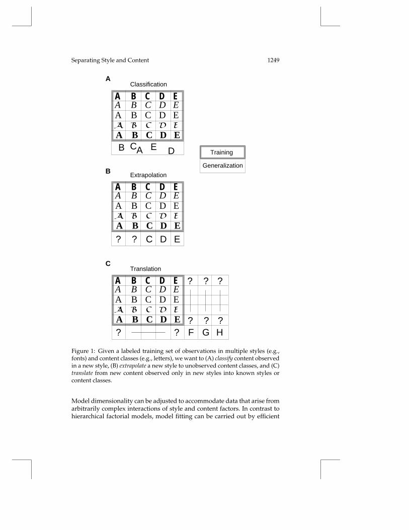
Figure 1 illustrates three abstract tasks that fall under this framework:classification, extrapolation, and translation. Examples of these abstract tasksin the domain of typography include classifying known characters in anovel font, extrapolating the missing characters of an incomplete novel font,or translating novel characters from a novel font into a familiar font. Theessential challenge in all of these tasks is the same. A perceptual systemobserves a training set of data in multiple styles and content classes and isthen presented with incomplete data in an unfamiliar style, missing eithercontent labels (see Figure 1A) or whole observations (see Figure 1B) or both(see Figure 1C). The system must generate the missing labels or observationsusing only the available data in the new style and what it can learn about theinteracting roles of style and content from the training set of complete data.
We describe a unified approach to the learning problems of Figure 1based on fitting models that discover explicit parameterized representationsof what the training data of each row have in common independent ofcolumn, what the data of each column have in common independent ofrow, and what all data have in common independent of row and column—the interaction of row and column factors. Such a modular representationnaturally supports generalization to new styles or content. For example, wecan extrapolate a new style to unobserved content classes (see Figure 1B)by combining content and interaction parameters learned during trainingwith style parameters estimated from available data in the new style.
Several models for the underlying factors of observations have recentlybeen proposed in the literature on unsupervised learning. These includeessentially additive factor models, as used in principal component analysis(Mardia et al., 1979), independent component analysis (Bell & Sejnowski,1995), and cooperative vector quantization (Hinton & Zemel, 1994; Ghahra-mani, 1995), and hierarchical factorial models, as used in the Helmholtz ma-chine and its descendants (Hinton et al., 1995; Dayan et al., 1995; Hinton &Ghahramani, 1997).
We model the mapping from style and content parameters to observa-tions as a bilinear mapping. Bilinear models are two-factor models with themathematical property of separability: their outputs are linear in either fac-tor when the other is held constant. Their combination of representationalexpressiveness and efficient learning procedures enables bilinear modelsto overcome two principal drawbacks of existing factor models that mightbe applied to learning the tasks in Figure 1. In contrast to additive factormodels, bilinear models provide for rich factor interactions by allowing fac-tors to modulate each other’s contributions multiplicatively (see section 2).
Separating Style and Content 1249
? ? C D E
Extrapolation
A B C D EA B C D EA B C D EA B C D EA B C D E
? ? F G H
? ? ?Translation
A B C D EA B C D EA B C D EA B C D EA B C D E ? ? ?
AB C DE
Classification
A B C D EA B C D EA B C D EA B C D EA B C D E
A
C
BGeneralization
Training
Figure 1: Given a labeled training set of observations in multiple styles (e.g.,fonts) and content classes (e.g., letters), we want to (A) classify content observedin a new style, (B) extrapolate a new style to unobserved content classes, and (C)translate from new content observed only in new styles into known styles orcontent classes.
Model dimensionality can be adjusted to accommodate data that arise fromarbitrarily complex interactions of style and content factors. In contrast tohierarchical factorial models, model fitting can be carried out by efficient
1250 Joshua B. Tenenbaum and William T. Freeman
techniques well known from the study of linear models, such as the singularvalue decomposition (SVD) and the expectation-maximization (EM) algo-rithm, without having to invoke extensive stochastic (Hinton et al., 1995) ordeterministic (Dayan et al., 1995) approximations.
Our approach is also related to the “learning-to-learn” research program(Thrun & Pratt, 1998)—also known as task transfer or multitask learning(Caruana, 1998). The central insight of “learning to learn” is that learningproblems often come in clusters of related tasks, and thus learners mayautomatically acquire useful biases for a novel learning task by trainingon many related ones. Rather than families of related tasks, we focus onhow learners can exploit the structure in families of related observations,bound together by their common styles, content classes, or style × contentinteraction, to acquire general biases useful for carrying out tasks on novelobservations from the same family. Thus, our work is closest in spirit tothe family discovery approach of Omohundro (1995), differing primarily inour focus on bilinear models to parameterize the style × content interac-tion.
Section 2 explains and motivates our bilinear modeling approach. Sec-tion 3 describes how these models are fit to a training set of observations.Sections 4, 5, and 6 present specific applications of these techniques to thethree tasks of classification, extrapolation, and translation, using realisticdata from three different perceptual domains. Section 7 suggests directionsfor future work, and section 8 offers some concluding comments.
We will use the terms style and content generically to refer to any twoindependent factors underlying a set of perceptual observations. For tasksthat require generalization to novel classes of only one factor (see Figures 1Aand 1B), we will refer to the variable factor (which changes during gener-alization) as style and the invariant factor (with a fixed set of classes) ascontent. For example, in a task of recognizing familiar words spoken in anunfamiliar accent, we would think of the words as content and the accentas style. For tasks that require generalization across both factors (see Fig-ure 1C), the labels style and content are arbitrary, and we will use them asseems most natural.
2 Bilinear Models
We have explored two bilinear models, closely related to each other, whichwe distinguish by the labels symmetric and asymmetric. This section describesthe two models and illustrates them on a simple data set of face images.
2.1 Symmetric Model. In the symmetric model, we represent both styles and content c with vectors of parameters, denoted as and bc and withdimensionalities I and J, respectively. Let ysc denote a K-dimensional obser-vation vector in style s and content class c. We assume that ysc is a bilinear

Separating Style and Content 1251
function of as and bc given most generally by the form
ysck =
I∑i=1
J∑j=1
wijkasi b
cj . (2.1)
Here i, j, and k denote the components of style, content, and observationvectors, respectively.1 The wijk terms are independent of style and contentand characterize the interaction of these two factors. Their meaning becomesclearer when we rewrite equation 2.1 in vector form. Letting Wk denote theI × J matrix with entries {wijk}, equation 2.1 can be written as
ysck = asT
Wkbc. (2.2)
In equation 2.2, the K matrices Wk describe a bilinear map from the styleand content vector spaces to the K-dimensional observation space.
The interaction terms have another interpretation, which can be seenby writing the symmetric model in a different vector form. Letting wij de-note the K-dimensional vector with components {wijk}, equation 2.1 can bewritten as
ysc =∑
i,j
wijasi b
cj . (2.3)
In equation 2.3, the wijk terms represent I × J basis vectors of dimension K,and the observation ysc is generated by mixing these basis vectors withcoefficients given by the tensor product of as and bc.
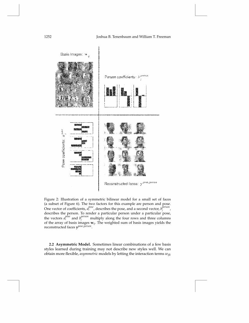
Of course, all of these interpretations are formally equivalent, but theysuggest different intuitions which we will exploit later. As a concrete exam-ple, Figure 2 illustrates a symmetric model of face images of different peoplein different poses (sampled from the complete data in Figure 6). Here thebasis vector interpretation of the wijk terms is most natural, by analogy to thewell-known work on eigenfaces (Kirby & Sirovich, 1990; Turk & Pentland,1991). Each pose is represented by a vector of I parameters, apose
i , and eachperson by a vector of J parameters, bperson
j . To render an image of a particularperson in a particular pose, a set of I × J basis images wij is linearly mixedwith coefficients given by the tensor product of these two parameter vectors(see equation 2.3). The symmetric model can exactly reproduce the obser-vations when I and J equal the numbers of observed styles S and contentclasses C, respectively, as is the case in Figure 2. The model provides coarserbut more compact representations as these dimensionalities are decreased.
1 The model in equation 2.1 may appear trilinear, but we view the wijk terms as de-scribing a fixed bilinear mapping from as and bc to ysc.
1252 Joshua B. Tenenbaum and William T. Freeman
Figure 2: Illustration of a symmetric bilinear model for a small set of faces(a subset of Figure 6). The two factors for this example are person and pose.One vector of coefficients, apose
i , describes the pose, and a second vector, bpersonj ,
describes the person. To render a particular person under a particular pose,the vectors apose
i and bpersonj multiply along the four rows and three columns
of the array of basis images wij. The weighted sum of basis images yields thereconstructed faces ypose,person.
2.2 Asymmetric Model. Sometimes linear combinations of a few basisstyles learned during training may not describe new styles well. We canobtain more flexible, asymmetric models by letting the interaction terms wijk

Separating Style and Content 1253
themselves vary with style. Then equation 2.1 becomes ysck =
∑i,j ws
ijkasi b
cj .
Without loss of generality, we can combine the style-specific terms of equa-tion 2.1 into
asjk =
∑i
wsijkas
i , (2.4)
giving
ysck =
∑j
asjkbc
j . (2.5)
Again, there are two interpretations of the model, corresponding to differentvector forms of equation 2.5. First, letting As denote the K × J matrix withentries {as
jk}, equation 2.5 can be written as
ysc = Asbc. (2.6)
Here, we can think of the asjk terms as describing a style-specific linear map
from content space to observation space. Alternatively, letting asj denote the
K-dimensional vector with components {asjk}, equation 2.5 can be written as
ysc =∑
j
asj bc
j . (2.7)
Now we can think of the asjk terms as describing a set of J style-specific
basis vectors that are mixed according to content-specific coefficients bcj
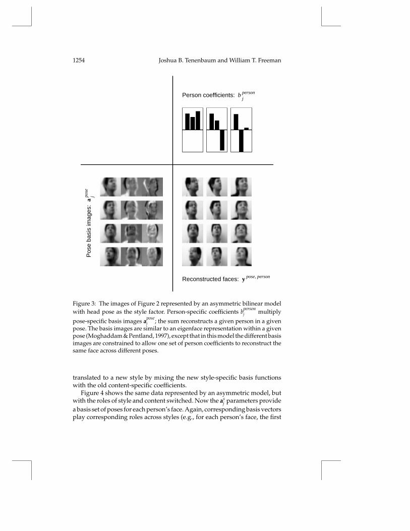
(independent of style) to produce the observations.Figure 3 illustrates an asymmetric bilinear model applied to the face
database, with head pose as the style factor. Each pose is represented bya set of J basis images apose
j and each person by a vector of J parameters
bpersonj . To render an image of a particular person in a particular pose, the
pose-specific basis images are linearly mixed with coefficients given by theperson-specific parameter vector.
Note that the basis images for each pose look like eigenfaces (Turk &Pentland, 1991) in the appropriate style of each pose. However, they do notprovide a true orthogonal basis for any one pose, as in Moghaddam andPentland (1997), where a distinct set of eigenfaces is computed for each ofseveral poses. Instead, the factorized structure of the model ensures thatcorresponding basis vectors play corresponding roles across poses (e.g., thefirst vector holds roughly the mean face for that pose, the second seemsto modulate hair distribution, and the third seems to modulate head size),which is crucial for adapting to new styles. Familiar content can be easily
1254 Joshua B. Tenenbaum and William T. Freeman
Reconstructed faces: y pose, person
Pos
e ba
sis
imag
es:
a po
se j
Person coefficients: b person j
Figure 3: The images of Figure 2 represented by an asymmetric bilinear modelwith head pose as the style factor. Person-specific coefficients bperson
j multiply
pose-specific basis images aposej ; the sum reconstructs a given person in a given
pose. The basis images are similar to an eigenface representation within a givenpose (Moghaddam & Pentland, 1997), except that in this model the different basisimages are constrained to allow one set of person coefficients to reconstruct thesame face across different poses.
translated to a new style by mixing the new style-specific basis functionswith the old content-specific coefficients.
Figure 4 shows the same data represented by an asymmetric model, butwith the roles of style and content switched. Now the as
j parameters providea basis set of poses for each person’s face. Again, corresponding basis vectorsplay corresponding roles across styles (e.g., for each person’s face, the first

Separating Style and Content 1255
Pose coefficients: b pose j
Reconstructed faces: y person, posePer
son
basi
s im
ages
: a
pe
rso
n j
Figure 4: Asymmetric bilinear model applied to the data of Figure 2, treatingidentity as the style factor. Now pose-specific coefficients bpose
j weight person-
specific basis images apersonj to reconstruct the face data. Across different faces,
corresponding basis images play corresponding roles in rotating head position.
vector holds roughly the mean pose, the second modulates head orientation,the third modulates amount of hair showing, and the fourth adds in facialdetail), allowing ready stylistic translation.
Finally, we note that because the asymmetric model can be obtained bysumming out redundant degrees of freedom in the symmetric model (seeequation 2.4),2 the three sets of basis images in Figures 2 through 4 arenot at all independent. Both the pose- and person-specific basis images inFigures 3 and 4 can be expressed as linear combinations of the symmetricmodel basis images in Figure 2, mixed according to the pose- or person-specific coefficients (respectively) from Figure 2.
The asymmetric model’s high-dimensional matrix representation of stylemay be too flexible in adapting to data in new styles and cannot support
2 This holds exactly only when the dimensionalities of style and content vectors areequal to the number of observed styles and content classes, respectively.
1256 Joshua B. Tenenbaum and William T. Freeman
translation tasks (see Figure 1C) because it does not explicitly model thestructure of observations that is independent of both style and content (rep-resented by wijk in equation 2.1). However, if overfitting can be controlledby limiting the model dimensionality J or imposing some additional con-straint, asymmetric models may solve classification and extrapolation tasks(see Figures 1A and 1B) that could not be solved using symmetric modelswith a realistic number of training styles.
3 Model Fitting
In conventional supervised learning situations, the data are divided intocomplete training patterns and incomplete (e.g., unlabeled) test patterns,which are assumed to be sampled randomly from the same distribution(Bishop, 1995). Learning then consists of fitting a model to the training datathat allows the missing aspects of the test patterns (e.g., class labels in aclassification task) to be filled in given the available information. The tasksin Figure 1, however, require that the learner generalize from training datasampled according to one distribution (i.e., in one set of styles and contentclasses) to test data drawn from a different but related distribution (i.e., ina different set of styles or content classes).
Because of the need to adapt to a different but related distribution ofdata during testing, our approach to these tasks involves model fitting dur-ing both training and testing phases. In the training phase, we learn aboutthe interaction of style and content factors by fitting a bilinear model to acomplete array of observations of C content classes in S styles. In the test-ing or generalization phase, we adapt the same model to new observationsthat have something in common with the training set, in either content orstyle or in their interaction. The model parameters corresponding to the as-sumed commonalities are fixed at the values learned during training, andnew parameters are estimated for the new styles or content using algorithmssimilar to those used in training. New and old parameters are then com-bined to accomplish the desired classification, extrapolation, or translationtask.
This section presents the basic algorithms for model fitting during train-ing. The algorithms for model fitting during testing are essentially variantsof these training algorithms but are task-specific; they will be presented inthe appropriate sections below.
The goal of model fitting during training is to minimize the total squarederror over the training set for the symmetric or asymmetric models. Thisgoal is equivalent to maximum likelihood estimation of the style and contentparameters given the training data, under the assumption that the data weregenerated from the models plus independently and identically distributedgaussian noise.
Separating Style and Content 1257
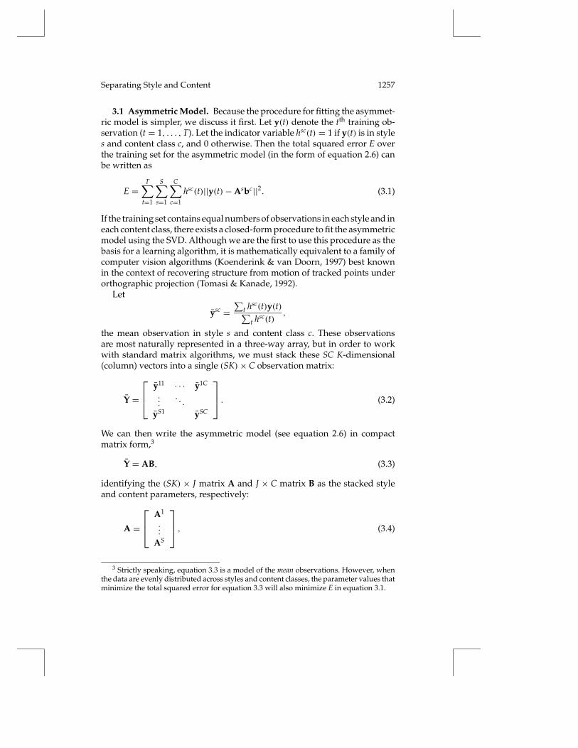
3.1 Asymmetric Model. Because the procedure for fitting the asymmet-ric model is simpler, we discuss it first. Let y(t) denote the tth training ob-servation (t = 1, . . . ,T). Let the indicator variable hsc(t) = 1 if y(t) is in styles and content class c, and 0 otherwise. Then the total squared error E overthe training set for the asymmetric model (in the form of equation 2.6) canbe written as
E =T∑
t=1
S∑s=1
C∑c=1
hsc(t)||y(t)−Asbc||2. (3.1)
If the training set contains equal numbers of observations in each style and ineach content class, there exists a closed-form procedure to fit the asymmetricmodel using the SVD. Although we are the first to use this procedure as thebasis for a learning algorithm, it is mathematically equivalent to a family ofcomputer vision algorithms (Koenderink & van Doorn, 1997) best knownin the context of recovering structure from motion of tracked points underorthographic projection (Tomasi & Kanade, 1992).
Let
ysc =∑
t hsc(t)y(t)∑t hsc(t)
,
the mean observation in style s and content class c. These observationsare most naturally represented in a three-way array, but in order to workwith standard matrix algorithms, we must stack these SC K-dimensional(column) vectors into a single (SK)× C observation matrix:
Y =
y11 · · · y1C
.... . .
yS1 ySC
. (3.2)
We can then write the asymmetric model (see equation 2.6) in compactmatrix form,3
Y = AB, (3.3)
identifying the (SK) × J matrix A and J × C matrix B as the stacked styleand content parameters, respectively:
A =
A1
...
AS
, (3.4)
3 Strictly speaking, equation 3.3 is a model of the mean observations. However, whenthe data are evenly distributed across styles and content classes, the parameter values thatminimize the total squared error for equation 3.3 will also minimize E in equation 3.1.
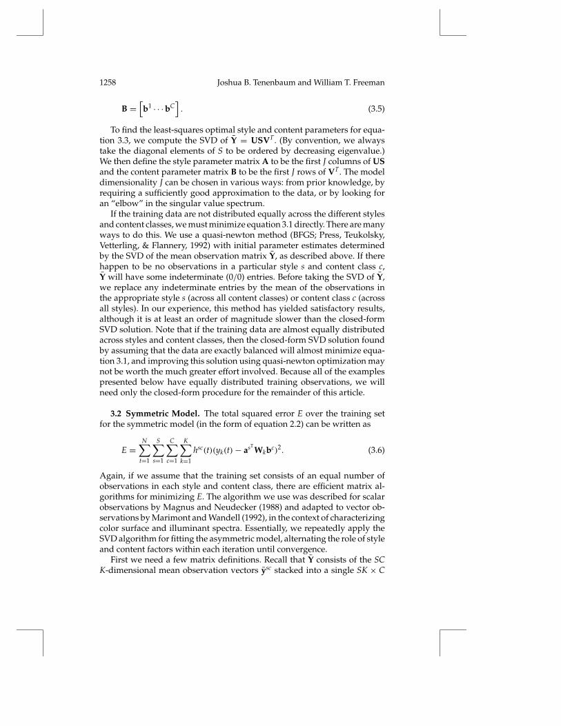
1258 Joshua B. Tenenbaum and William T. Freeman
B =[b1 · · ·bC
]. (3.5)
To find the least-squares optimal style and content parameters for equa-tion 3.3, we compute the SVD of Y = USVT. (By convention, we alwaystake the diagonal elements of S to be ordered by decreasing eigenvalue.)We then define the style parameter matrix A to be the first J columns of USand the content parameter matrix B to be the first J rows of VT. The modeldimensionality J can be chosen in various ways: from prior knowledge, byrequiring a sufficiently good approximation to the data, or by looking foran “elbow” in the singular value spectrum.
If the training data are not distributed equally across the different stylesand content classes, we must minimize equation 3.1 directly. There are manyways to do this. We use a quasi-newton method (BFGS; Press, Teukolsky,Vetterling, & Flannery, 1992) with initial parameter estimates determinedby the SVD of the mean observation matrix Y, as described above. If therehappen to be no observations in a particular style s and content class c,Y will have some indeterminate (0/0) entries. Before taking the SVD of Y,we replace any indeterminate entries by the mean of the observations inthe appropriate style s (across all content classes) or content class c (acrossall styles). In our experience, this method has yielded satisfactory results,although it is at least an order of magnitude slower than the closed-formSVD solution. Note that if the training data are almost equally distributedacross styles and content classes, then the closed-form SVD solution foundby assuming that the data are exactly balanced will almost minimize equa-tion 3.1, and improving this solution using quasi-newton optimization maynot be worth the much greater effort involved. Because all of the examplespresented below have equally distributed training observations, we willneed only the closed-form procedure for the remainder of this article.
3.2 Symmetric Model. The total squared error E over the training setfor the symmetric model (in the form of equation 2.2) can be written as
E =N∑
t=1
S∑s=1
C∑c=1
K∑k=1
hsc(t)(yk(t)− asTWkbc)2. (3.6)
Again, if we assume that the training set consists of an equal number ofobservations in each style and content class, there are efficient matrix al-gorithms for minimizing E. The algorithm we use was described for scalarobservations by Magnus and Neudecker (1988) and adapted to vector ob-servations by Marimont and Wandell (1992), in the context of characterizingcolor surface and illuminant spectra. Essentially, we repeatedly apply theSVD algorithm for fitting the asymmetric model, alternating the role of styleand content factors within each iteration until convergence.
First we need a few matrix definitions. Recall that Y consists of the SCK-dimensional mean observation vectors ysc stacked into a single SK × C

Separating Style and Content 1259
A B
Figure 5: Schematic illustration of the vector transpose (following Marimont &Wandell, 1992). For a matrix Y considered as a two-dimensional array of stackedvectors (A), its vector-transpose YVT is defined to be the same stacked vectorswith their row and column positions in the array transposed (B).
matrix (see equation 3.2). In general, for any AK × B matrix X constructedby stacking AB K-dimensional vectors A down and B across, we can defineits vector transpose XVT to be the BK × A matrix consisting of the same K-dimensional vectors stacked B down and A across, where the vector a acrossand b down in X becomes the vector b across and a down of XVT (see Figure 5).In particular, YVT consists of the means ysc stacked into a single (KC) × Smatrix:
YVT =
y11 · · · y1S
.... . .
yC1 yCS
. (3.7)
Finally, we define the IK × J stacked weight matrix W, consisting of theIJ K-dimensional basis functions wij (see equation 2.3) in the form
W =
w11 · · · w1J...
. . .
wI1 wIJ
. (3.8)
Its vector transpose WVT is also defined accordingly.

1260 Joshua B. Tenenbaum and William T. Freeman
We can then write the symmetric model (see equation 2.6) in either ofthese two equivalent matrix forms,4
Y =[WVTA
]VTB, (3.9)
YVT = [WB]VT A, (3.10)
identifying the I × S matrix A and the J × C matrix B as the stacked styleand content parameter vectors, respectively:
A =[a1 · · · aS
],B =
[b1 · · ·bC
]. (3.11)
The iterative procedure for estimating least-squares optimal values of Aand B proceeds as follows. We initialize B using the closed-form SVD pro-cedure described above for the asymmetric model (see equation 3.5). Notethat this initial B is an orthogonal matrix (BBT is the J × J identity matrix),so that [YBT]VT = WVTA (from equation 3.9). Thus, given this initial esti-mate for B, we can compute the SVD of [YBT]VT = USVT and update ourestimate of A to be the first I rows of VT. This A is also orthogonal, so that[YVTAT]VT = WB (from equation 3.10). Thus, given this estimate of A, wecan compute the SVD of [YVTAT]VT = USVT and update our estimate of Bto be the first J rows of VT. This completes one iteration of the algorithm.Typically, convergence occurs within five iterations (around 10 SVD opera-tions). Convergence is also guaranteed. (See Magnus & Neudecker, 1988, fora proof for the scalar case, K = 1, which can be extended to the vector caseconsidered here.) Upon convergence, we solve for W = [[YBT]VTAT]VT toobtain the basis vectors independent of both style and content. As with theasymmetric model, if the training data are not distributed equally across thedifferent styles and content classes, we minimize equation 3.1 starting fromthe same initial estimates for A and B but using a more costly quasi-Newtonmethod.
4 Classification
Many common classification problems involve multiple observations likelyto be in one style, for example, recognizing the handwritten characters onan envelope or the accented speech of a telephone voice. People are sig-nificantly better at recognizing a familiar word spoken in an unfamiliarvoice or a familiar letter character written in an unfamiliar font when it isembedded in the context of other words or letters in the same novel style
4 As with the asymmetric model, when the data are evenly distributed across stylesand content classes, the parameter values that minimize the total squared error for themean observations in equations 3.9 and 3.10 will also minimize E in Equation 3.6.

Separating Style and Content 1261
(van Bergem, Pols, & van Beinum, 1988; Sanocki, 1992; Nygaard & Pisoni,1998), presumably because the added context allows the perceptual systemto build a model of the new style and factor out its influence.
In this section, we show how a perceptual system may use bilinear mod-els and assumptions of style consistency to factor out the effects of style incontent classification and thereby significantly improve classification per-formance on data in novel styles. We first describe the two concrete tasksinvestigated. We then present the general classification algorithm and theresults of several experiments comparing this algorithm to standard tech-niques from the pattern recognition literature, such as nearest neighborclassification, which do not explicitly model the effects of style on contentclassification.
4.1 Task Specifics. We report experiments with two data sets: a bench-mark speech data set and a face data set that we collected ourselves. Thespeech data consist of six samples of each of 11 vowels (content classes) ut-tered by 15 speakers (styles) of British English.5 Each data vector consists ofK = 10 log area parameters, a standard vocal tract representation computedfrom a linear predictive coding analysis of the digitized speech. The specifictask we must learn to perform is classification of spoken vowels (content)for new speakers (styles).
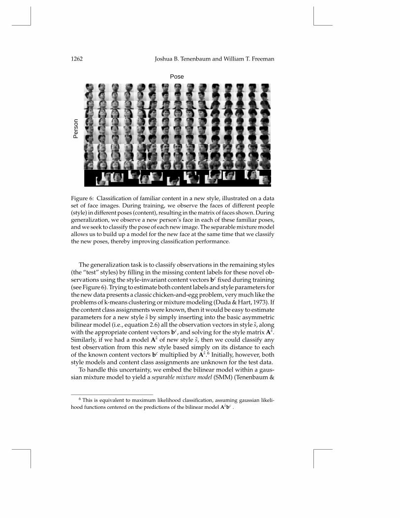
The face data were introduced in section 2 (see Figures 2–4). Figure 6shows the complete data set, consisting of images of 11 people’s faces (styles)viewed under 15 different poses (content classes). The poses span a grid ofthree vertical positions (up, level, down) and five horizontal positions (farleft, left, straight ahead, right, far right). The pictures were shifted to alignthe nose tip position, found manually. The images were then blurred andcropped to 22×32 pixels, and represented simply as vectors of K = 704 pixelvalues each. The specific task we must learn to perform is classification ofhead pose (content) for new people’s faces (styles).
4.2 Algorithm. For both speech and face data sets, we train on observa-tions in all content classes but in a subset of the available styles (the “train-ing” styles). We fit asymmetric bilinear models (see equation 3.3) to thesetraining data using the closed-form SVD procedure described in section 3.1.This yields a K × J matrix As representing each style s and a J-dimensionalvector bc representing each content class c. The model dimensionality J is afree parameter, which we discuss in depth at the end of this section. Fittingthese asymmetric models to either data set required less than 1 second. Thisand all other execution times reported below were obtained for nonopti-mized MATLAB code running on a Silicon Graphics O2 workstation.
5 The data were originally collected by David Deterding and are now available onlinefrom the UC Irvine machine learning repository (http://www.ics.uci.edu/∼mlearn).
1262 Joshua B. Tenenbaum and William T. Freeman
PoseP
erso
n
Figure 6: Classification of familiar content in a new style, illustrated on a dataset of face images. During training, we observe the faces of different people(style) in different poses (content), resulting in the matrix of faces shown. Duringgeneralization, we observe a new person’s face in each of these familiar poses,and we seek to classify the pose of each new image. The separable mixture modelallows us to build up a model for the new face at the same time that we classifythe new poses, thereby improving classification performance.
The generalization task is to classify observations in the remaining styles(the “test” styles) by filling in the missing content labels for these novel ob-servations using the style-invariant content vectors bc fixed during training(see Figure 6). Trying to estimate both content labels and style parameters forthe new data presents a classic chicken-and-egg problem, very much like theproblems of k-means clustering or mixture modeling (Duda & Hart, 1973). Ifthe content class assignments were known, then it would be easy to estimateparameters for a new style s by simply inserting into the basic asymmetricbilinear model (i.e., equation 2.6) all the observation vectors in style s, alongwith the appropriate content vectors bc, and solving for the style matrix As.Similarly, if we had a model As of new style s, then we could classify anytest observation from this new style based simply on its distance to eachof the known content vectors bc multiplied by As.6 Initially, however, bothstyle models and content class assignments are unknown for the test data.
To handle this uncertainty, we embed the bilinear model within a gaus-sian mixture model to yield a separable mixture model (SMM) (Tenenbaum &
6 This is equivalent to maximum likelihood classification, assuming gaussian likeli-hood functions centered on the predictions of the bilinear model Asbc .
Separating Style and Content 1263
Freeman, 1997), which can then be fit efficiently to new data using the EMalgorithm (Dempster, Laird, & Rubin, 1977). The mixture model has S × Cgaussian components—one for each pair of S styles and C content classes—with means given by the predictions of the bilinear model. However, onlyon the order of (S + C) parameters are needed to represent the means ofthese S × C gaussians, because of the bilinear model’s separable structure.To classify known content in new styles and estimate new style parame-ters simultaneously, the EM algorithm alternates between calculating theprobabilities of all content labels given current style parameter estimates(E-step) and estimating the most likely style parameters given current con-tent label probabilities (M-step), with likelihood determined by the gaussianmixture model. If, in addition, the test data are not segmented according tostyle, style label probabilities can be calculated simultaneously as part ofthe E-step.
More formally, after training on labeled data from S styles and C contentclasses, we are given test data from the same C content classes and S newstyles, with labels for content (and possibly also style) missing. The newstyle matrices As are also unknown, but the content vectors bc are known,having been fixed in the training phase. We assume that the probabilityof a new unlabeled observation y being generated in new style s and oldcontent c is given by a gaussian distribution with variance σ 2 centered atthe prediction of the bilinear model: p(y|s, c) ∝ exp{−‖y − Asbc‖2/(2σ 2)}.The total probability of y is then given by the mixture distribution p(y) =∑
s,c p(y|s, c)p(s, c). Here we assume equal prior probabilities p(s, c), unlessthe observations are otherwise labeled.7 The EM algorithm (Dempster et al.,1977) alternates between two steps in order to find new style matrices As
and style-content labels p(s, c|y) that best explain the test data. In the E-step,we compute the probabilities p(s, c|y) = p(y|s, c)p(s, c)/p(y) that each testvector y belongs to style s and content class c, given the current style matrixestimates. In the M-step, we estimate new style matrices by setting As tomaximize the total log-likelihood of the test data, L∗ =∑y log p(y). The M-step can be computed in closed form by solving the equations ∂L∗/∂As = 0,which are linear in As given the probability estimates from the E-step andthe quantities msc =∑y p(s, c|y)y and nsc =∑y p(s, c|y):
As =[∑
cmscbcT
][∑c
nscbcbcT
]−1
. (4.1)
The EM algorithm is guaranteed to converge to a local maximum of L∗,and this typically takes around 20 iterations for our problems. After each
7 That is, if the style identity s∗ of y is labeled but the content class is unknown, welet p(s, c) = 1/C if s = s∗ and 0 if s 6= s∗. If both the style and content identities of y areunlabeled, we let p(s, c) = 1/(SC) for all s and c.

1264 Joshua B. Tenenbaum and William T. Freeman
E-step, test vectors in new styles can be classified by selecting the contentclass c that maximizes p(c|y) = ∑
s p(s, c|y).8 Classification performanceis determined by the percentage of test data for which the probability ofcontent class c, as given by EM, is greatest for the actual content class.Note that because content classification is determined as a by-product ofthe E-step, the standard practice of running EM until convergence to a localmaximum in likelihood will not necessarily lead to optimal classificationperformance. In fact, we have often observed overfitting behavior, in whichoptimal classification is obtained after only two or three iterations of EM, butthe likelihood continues to increase in subsequent iterations as observationsare assigned to incorrect content classes.
This classification algorithm thus has three free parameters for whichgood values must somehow be determined. In addition to the model dimen-sionality J mentioned above, these parameters include the model varianceσ 2 and the maximum number of iterations for which EM is run, tmax. In gen-eral, we set these parameters using a leave-one-style-out cross-validationprocedure with the training data. That is, given S complete training styles,we train separate bilinear models on each of the S subsets of S − 1 stylesand evaluate these models’ classification performance on the one style thateach was not trained on. For each of these S training set splits, we try arange of values for the parameters J, σ 2, and tmax. Those values that yieldthe best average performance over the S training set splits are then used infitting a new bilinear model to the full training data and generalizing to thedesignated test set. The main drawback of this cross-validation procedureis that it can be time-consuming. Although each run of EM is quite fast—onthe order of seconds—an exhaustive search of the full parameter space ina leave-one-out design may take hours. In real applications, such a searchwould hopefully need to be done only once in a given domain, if at all, andmight also be guided by domain-specific knowledge that could narrow thesearch space significantly.
Initialization is an important factor in determining the success of the EMalgorithm. Because we are primarily interested in good classification, weinitialize EM in the E-step, using the results of a simple 1-nearest-neighborclassifier to set the content-class assignments p(c|x). That is, we initiallyassign each test observation to the content class of the most similar trainingobservation (for which the content labels are known).
4.3 Results. We conducted four experiments: three using the benchmarkspeech data to investigate different aspects of the algorithm’s behavior andone using the face data to provide evidence from a separate domain. Ineach case, we report results with all three free parameters set using the
8 If the style s∗ of y is known, then p(s, c|y) = 0 for all s 6= s∗ (see previous note). Inthat case, p(c|y) is simply equal to p(s∗, c|y).

Separating Style and Content 1265
Table 1: Accuracy of Classifying Spoken Vowels from a Benchmark Multi-speaker Database.
Classifier Percentage Correcton Test Data
Multilayer perceptron (MLP) 51%Radial basis function network (RBF) 53%1-nearest neighbor (1-NN) 56%Discriminant adaptive nearest neighbor (DANN)
Generic parameter settings 59.7%Optimal parameter settings 61.7%
Separable mixture models (SMM)—test speakers labeledAll parameters set by CV (J = 3, σ 2 = 1/64, tmax = 2) 75.8%tmax = ∞; J, σ 2 set by CV (J = 3, σ 2 = 1/32) 68.2%tmax = ∞; optimal J, σ 2 (J = 4, σ 2 = 1/16) 77.3%
Separable mixture models (SMM)—test speakers not labeledAll parameters set by CV (J = 3, σ 2 = 1/64, tmax = 2) 69.8%± .3%tmax = ∞; J, σ 2 set by CV (J = 3, σ 2 = 1/32) 59.9%± 1.1%tmax = ∞; optimal J, σ 2 (J = 3, σ 2 = 1/64) 63.2%± 1.5%
Notes: MLP, RBF, and 1-NN results were obtained by Robinson (1989). The DANNclassifier (Hastie & Tibshirani, 1996) achieves the best performance we know of for anapproach that does not adapt to new speakers. The SMM classifiers perform signif-icantly better vowel classification by simultaneously modeling speaker style. “CV”denotes the cross-validation procedure for parameter setting described in the text.
cross-validation procedure described above, as well as for two conditionsin which EM was run until convergence (tmax = ∞): both J and σ 2 deter-mined by cross validation and both J and σ 2 set to their optimal values (asan indicator of best in-principle performance for the maximum likelihoodsolution).
4.3.1 Train 8, Test 7 on Speech Data—Speakers Labeled. The first experi-ment with the speech data was the standard benchmark task described inRobinson (1989). Robinson compared many learning algorithms trained tocategorize vowels from the first eight speakers (four male and four female)and tested on samples from the remaining seven speakers (four male andthree female). The variety and the small number of styles make this a diffi-cult task. Table 1 shows the best results we know of for standard approachesthat do not adapt to new speakers. Of the many techniques that Robinson(1989) tested, 1-nearest neighbor (1-NN) performs the best, with 56.3% cor-rect; chance is approximately 9% correct. The discriminant adaptive nearestneighbor (DANN) classifier (Hastie & Tibshirani, 1996) slightly outperforms1-NN, obtaining 59.7% correct with its generic parameter settings and 61.7%correct for optimal parameter settings.

1266 Joshua B. Tenenbaum and William T. Freeman
After fitting an asymmetric bilinear model to the training data, we testedclassification performance using our SMM on the seven new speakers’ data.We first assumed that style labels were available for the test data (indicatingonly a change of speaker, but no information about the new speaker’s style).Running EM until convergence (tmax = ∞), our best results of 77.3% correctwere obtained with J = 4 and σ 2 = 1/16. Almost comparable results of75.8% correct were obtained using cross-validation to set all parameters(J, σ 2, tmax) automatically (see Table 1). The SMM clearly outperforms themany nonadaptive techniques tested, exploiting extra information availablein the speaker labels that nonadaptive techniques make no use of.
4.3.2 Train 8, Test 7 on Speech Data—Speakers Not Labeled. We next re-peated the benchmark experiment without the assumption that any stylelabels were available during testing. Thus, our SMM algorithm and the non-adaptive techniques had exactly the same information available for each testobservation (although the SMM had style labels available during training).We used EM to figure out both the speaker assignments and the vowel classassignments for the test data. EM requires that the number of style compo-nents S in the mixture model be set in advance; we chose S = 7 (the actualnumber of distinct speakers) for consistency with the previous experiment.In initializing EM in the E-step, we assigned each test observation equallyto each new style component, plus or minus 10% random noise to breaksymmetry and allow each style component to adapt to a distinct subset ofthe new data. Using cross-validation to set J, σ 2, and tmax automatically, weobtained 69.8%± 0.3% correct. Table 1 presents results for other parametersettings. These scores reflect average performance over 10 random initial-izations. Not surprisingly, SMM performance here was worse than in theprevious section, where the correct style labels were assumed to be known.Nonetheless, the SMM still provided a significant improvement over thebest nonadaptive approaches tested.
4.3.3 Train 14, Test 1 on Speech Data. We noticed that the performance ofthe SMM on the speech data varied widely across different test speakers andalso depended significantly on the particular speakers chosen for trainingand testing. In some cases, the SMM did not perform much better than 1-NN, and in other cases the SMM actually did worse. Thus, we decided toconduct a more systematic study of the effects of individual speaker styleon generalization. Specifically, we tested the SMM’s ability to classify thespeech of each of the 15 speakers in the database individually when the other14 speakers were used for training. Because only one speaker was presentedduring testing, we used only a single style model in EM, and thus there wasno distinction between the “speakers labeled” and “speakers not labeled”conditions investigated in the previous two sections.
Averaged over all 15 possible test speakers, 1-NN obtained 63.9%±3.4%correct. Using cross-validation to set J, σ 2, and tmax automatically, our SMM
Separating Style and Content 1267
obtained 74.3%± 4.2% correct. Running EM until convergence (tmax = ∞),we obtained 75.6% ± 4.0% using the best parameter settings of J = 11,σ 2 = .01, and 73.5%± 4.4% correct using cross-validation to select J and σ 2
automatically. These SMM scores are not significantly different from eachother but are all significantly higher than 1-NN as measured by paired t-tests (p < .01 in all cases). The results suggest that the superior performanceof SMM over nonadaptive classifiers such as nearest neighbor will hold ingeneral over a range of different test styles.
This experiment also provided an opportunity to assess systematicallythe performance details of EM on the task of speech classification. For all15 possible test speakers, EM converged within 30 iterations, taking lessthan 5 seconds. The optimal number of iterations for EM as determined bycross-validation was always between 1 and 10 iterations, with a mean of3.2 iterations. We can assess the chance of falling into a bad local minimumwith EM by comparing the classification performance of the SMM fit usingEM with the performance of 1-NN on a speaker-by-speaker basis. For 14 of15 test speakers, the SMM consistently obtained better classification ratesthan 1-NN, regardless of which of the three parameter-setting proceduresdescribed above was used. The remaining speaker was always classifiedbetter by 1-NN. Evidently the vast majority of stylistic variations in thisdomain can be successfully modeled by the SMM and separated from therelevant content to be classified using the EM algorithm.
4.3.4 Train 10, Test 1 on Face Data. To provide further support for thegeneral advantage of SMM over nonadaptive approaches, we replicatedthe previous experiment using the face database instead of the speech data.Although the two databases are of roughly comparable size, the nature ofthe observations is quite different: 704-dimensional vectors of pixel valuesversus 10-dimensional vectors of vocal tract log area coefficients. Specifi-cally, we tested the SMM’s ability to classify head pose for each of the 11faces in the database individually when the other 10 people’s faces wereused for training. There were 15 possible poses, with one image of each facein each pose.
Averaged over all 11 possible test faces, 1-NN obtained 53.9%±4.3% cor-rect. Using cross-validation to set J, σ 2, and tmax automatically, our SMM ob-tained 73.9%±6.7% correct. Running EM until convergence (tmax = ∞), weobtained 80.6%± 7.5% using the best parameter settings of J = 6, σ 2 = 105,and 75.8%±6.4% correct using cross-validation to select J and σ 2 automati-cally. As on the speech data, these SMM scores are not significantly differentfrom each other but do represent significant improvements over 1-NN asmeasured by paired t-tests (p < .05 in all cases).
The performance details of EM on this face classification task were quitesimilar to those on the speech classification task reported above. For all 11possible test faces, EM converged within 30 iterations, taking less than 20seconds. (The longer convergence times here reflect the higher-dimensional
1268 Joshua B. Tenenbaum and William T. Freeman
vectors involved.) The optimal number of iterations for EM as determinedby cross-validation was between 9 and 20 iterations, with a mean of 12.6iterations. For 9 of 11 test faces, the SMM consistently obtained better clas-sification rates than 1-NN over all three parameter-setting procedures weused, indicating that local minima do not prevent the EM algorithm fromfactoring out the majority of stylistic variations in this domain.
4.4 Discussion. Our approach to style-adaptive content classificationinvolves two significant modeling choices: the use of a bilinear model of themean observations and the use of a gaussian mixture model—centered onthe predictions of the bilinear model—for observations whose content orstyle assignments are unknown. The mixture model provides a principledprobabilistic framework, allowing us to use the EM algorithm to solve thechicken-and-egg problem of simultaneously estimating style parameters forthe new data and labeling the data according to content class (and possiblystyle as well). The bilinear structure of the model allows the M-step to becomputed in closed form by solving systems of linear equations. In thissense, bilinear models represent the content of observations independentof their style in a form that can be generalized easily to model data innew styles. To summarize our results, we found that separating style andcontent with bilinear models improves content classification in new stylessubstantially over the best nonadaptive approaches to classification, evenwhen no style information is available during testing, and dramaticallyso when style demarcation is available. Although our SMM classifier hasseveral free parameters that must be chosen a priori, we showed that near-optimal values can be determined automatically using a cross-validationtraining procedure. We obtained good results on two very different datasets, low-dimensional speech data and high-dimensional face image data,suggesting that our approach may be widely applicable to many two-factorclassification tasks that can be thought of in terms of recognizing invariantcontent elements under variable style.
5 Extrapolation
The ability to draw analogies across observations in different contexts is ahallmark of human perception and cognition (Hofstadter, 1995; Holyoak& Barnden, 1994). In particular, the ability to produce analogous contentin a novel style—and not just recognize it, as in the previous section—hasbeen taken as a severe test of perceptual abstraction (Hofstadter, 1995; Gre-bert, Stork, Keesing, & Mims, 1992). The domain of typography providesa natural place to explore these issues of analogy and production. Indeed,Hofstadter (1995) has argued that the question, “What is the letter ‘a’?” maybe “the central problem of AI” (p. 633). Following Hofstadter, we study thetask of extrapolating a novel font from an incomplete set of letter observa-tions in that font to the remaining unobserved letters. We first describe the

Separating Style and Content 1269
task specifics and our shape representation for letter observations. We thenpresent our algorithm for stylistic extrapolation based on bilinear modelsand show results on extrapolating a natural font.
5.1 Task Specifics. Given a training set of C = 62 characters (content)in S = 5 standard fonts (style), the task is to generate characters that arestylistically consistent with letters in a novel sixth font. The initial datawere obtained by digitizing the uppercase letters, lowercase letters, anddigits 0–9 of the six fonts at 38× 38 pixels using Adobe Photoshop. Success-ful shape modeling often depends on having an image representation thatmakes explicit the appropriate structure that is only implicit in raw pixelvalues. Specifically, the need to represent shapes of different topologies incomparable forms motivates using a particle-based representation (Szeliski& Tonnesen, 1992). We also want the letters in our representation to behavelike a linear vector space, where linear combinations of letters also look likeletters. Beymer and Poggio (1996) advocate a dense warp map for relatedproblems. Combining these two ideas, we chose to represent each lettershape by a 2× 38× 38 = 2888-dimensional vector of (horizontal and verti-cal) displacements that a set of 38 × 38 = 1444 ink particles must undergoto form the target shape from a reference grid.
With identical particles, there are many possible such warp maps. Toensure that similarly shaped letters are represented by similar warps, weuse a physical model. We give each particle of the reference shape (takento be the full rectangular bitmap) unit positive charge, and each pixel ofthe target letter negative charge proportional to its gray level intensity. Thetotal charge of the target letter is set equal to the total charge of the referenceshape. We track the electrostatic force lines from each particle of the referenceshape to where they intersect the plane of the target letter (see Figure 7A).The target shape is positioned opposite the reference shape, 100 pixel unitsaway in depth. The force lines land in a uniform density over the target letter,creating a correspondence between each ink particle of the reference shapeand a position on the target letter. The result is a smooth, dense warp mapspecifying a translation that each ink particle of the reference shape mustundergo to reassemble the collection of particles into the target letter shape(see Figure 7B). The electrostatic forces used to find the correspondences areeasily calculated from Coulomb’s law (Jackson, 1975). We call this a Coulombwarp representation. To render a warp map representation of a shape, we firsttranslate each particle of the reference shape by its warp map value, usinga grid at four times the linear pixel resolution. We then blur with a gaussian(standard deviation equal to five pixels) threshold the ink densities at 60% oftheir maximum and subsample to the original font resolution. By allowingnoninteger charge values and subpixel translations, we can preserve fontantialiasing information.
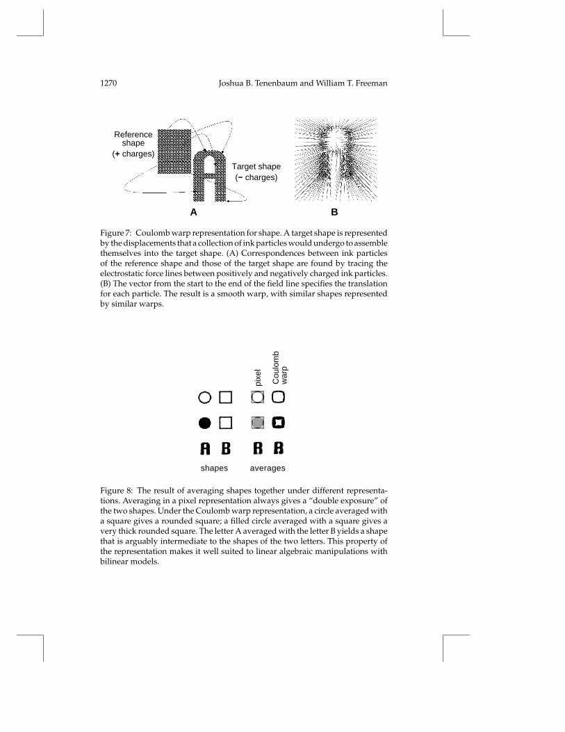
Figure 8 shows three pairs of shapes of different topologies, and theaverage of each pair in a pixel representation and in a Coulomb warp rep-
1270 Joshua B. Tenenbaum and William T. Freeman
Referenceshape
(+ charges)
A B
Target shape(− charges)
Figure 7: Coulomb warp representation for shape. A target shape is representedby the displacements that a collection of ink particles would undergo to assemblethemselves into the target shape. (A) Correspondences between ink particlesof the reference shape and those of the target shape are found by tracing theelectrostatic force lines between positively and negatively charged ink particles.(B) The vector from the start to the end of the field line specifies the translationfor each particle. The result is a smooth warp, with similar shapes representedby similar warps.
shapes
Cou
lom
bw
arp
pixe
l
averages
Figure 8: The result of averaging shapes together under different representa-tions. Averaging in a pixel representation always gives a “double exposure” ofthe two shapes. Under the Coulomb warp representation, a circle averaged witha square gives a rounded square; a filled circle averaged with a square gives avery thick rounded square. The letter A averaged with the letter B yields a shapethat is arguably intermediate to the shapes of the two letters. This property ofthe representation makes it well suited to linear algebraic manipulations withbilinear models.
Separating Style and Content 1271
resentation. Averaging the shapes in a pixel representation simply yields a“double exposure” of the two images; averaging in a Coulomb warp repre-sentation results in a shape intermediate to the two being averaged.
5.2 Algorithm. During training, we fit the asymmetric bilinear model(see equation 3.3) to five full fonts using the closed-form SVD procedure de-scribed in section 3.1. This yields a K× J matrix As representing each font sand a J-dimensional vector bc representing each letter class c, with the obser-vation dimensionality K = 2888. Training on this task took approximately48 seconds.
Adapting the model to an incomplete new style s can be carried out inclosed form using the content vectors bc learned during training. Supposewe observe M samples of style s, in content classes C = {c1, . . . , cM}. We findthe style matrix As that minimizes the total squared error over the test data,
E∗ =∑c∈C
‖ysc −Asbc‖2. (5.1)
The minimum of E∗ is found by solving the linear system ∂E∗/∂As = 0.Missing observations in the test style s and known content class c can thenbe synthesized from ysc = Asbc.
In order to allow the model sufficient expressive range to produce natural-looking letter shapes, we set the model dimensionality J as high as possible.However, such a flexible model led to overfitting on the available letters ofthe test font and consequently poor synthesis of the missing letters in thatfont. To regularize the style fit to the test data and thereby avoid overfitting,we add a prior term to the squared-error cost of equation 5.1 that encour-ages As to be close to the linear combination of training style parametersA1, . . . ,AS, that best fits the test font. Specifically, let AOLC be the value ofAs that minimizes equation 5.1 subject to the constraint that AOLC is a linearcombination of the training style parameters As, that is, AOLC =∑S
s=1 αsAs
for some values of αs. (OLC stands for “optimal linear combination.”) With-out loss of generality, we can think of the αs coefficients as the best-fittingstyle parameters of a symmetric bilinear model with dimensionality I equalto the number of styles S. We then redefine E∗ to include this new cost,
E∗ =∑c∈C
‖ysc −Asbc‖2 + λ‖As −AOLC‖2, (5.2)
and again minimize E∗ by solving the linear system ∂E∗/∂As = 0. The trade-off between these two costs is determined by the free parameter λ, whichwe set by eye to yield results with the best appearance. For this example,we used a model dimensionality of 60 and λ = 2 × 104.9 All model fittingduring this testing phase took less than 10 seconds.
9 This large value of λwas necessary to compensate for the differences in scale between
1272 Joshua B. Tenenbaum and William T. Freeman
synthetic
actual
? ?
A
B
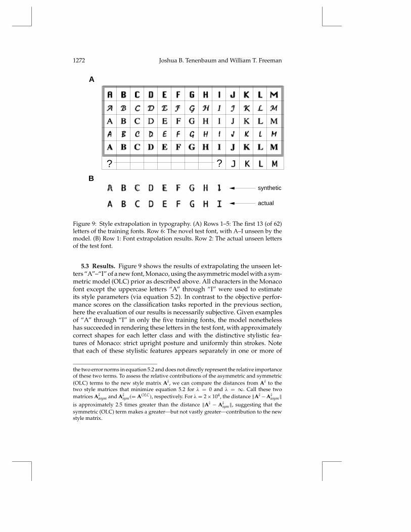
Figure 9: Style extrapolation in typography. (A) Rows 1–5: The first 13 (of 62)letters of the training fonts. Row 6: The novel test font, with A–I unseen by themodel. (B) Row 1: Font extrapolation results. Row 2: The actual unseen lettersof the test font.
5.3 Results. Figure 9 shows the results of extrapolating the unseen let-ters “A”–“I” of a new font, Monaco, using the asymmetric model with a sym-metric model (OLC) prior as described above. All characters in the Monacofont except the uppercase letters “A” through “I” were used to estimateits style parameters (via equation 5.2). In contrast to the objective perfor-mance scores on the classification tasks reported in the previous section,here the evaluation of our results is necessarily subjective. Given examplesof “A” through “I” in only the five training fonts, the model nonethelesshas succeeded in rendering these letters in the test font, with approximatelycorrect shapes for each letter class and with the distinctive stylistic fea-tures of Monaco: strict upright posture and uniformly thin strokes. Notethat each of these stylistic features appears separately in one or more of
the two error norms in equation 5.2 and does not directly represent the relative importanceof these two terms. To assess the relative contributions of the asymmetric and symmetric(OLC) terms to the new style matrix As, we can compare the distances from As to thetwo style matrices that minimize equation 5.2 for λ = 0 and λ = ∞. Call these twomatrices As
asym and Assym(= AOLC), respectively. For λ = 2× 10⁴, the distance ‖As−As
asym‖is approximately 2.5 times greater than the distance ‖As − As
sym‖, suggesting that thesymmetric (OLC) term makes a greater—but not vastly greater—contribution to the newstyle matrix.

Separating Style and Content 1273
pixel
rep.
asym
met
ric
sym
met
ric
asym
met
ric w
ith
sym
met
ric p
rior
actu
al
Figure 10: Result of different methods applied to the font extrapolation problem(Figure 9), where unseen letters in a new font are synthesized. The asymmetricbilinear model has too many parameters to fit, and generalization to new lettersis poor (second column). The symmetric bilinear model has only 5 degrees offreedom for our data and fails to represent the characteristics of the new font(third column). We used the symmetric model result as a prior to constrainthe flexibility of the asymmetric model, yielding the results shown here (fourthcolumn) and in Figure 9. All of these methods used the Coulomb warp repre-sentation for shape. Performing the same calculations in a pixel representationrequires blurring the letters so that linear combinations can modify shape, andyields barely passable results (first column). The far right column shows theactual letters of the new font.
the training fonts, but they do not appear together in any one trainingfont.
5.4 Discussion. We have shown that it is possible to learn the style ofa font from observations and extrapolate that style to unseen letters, us-ing a hybrid of asymmetric and symmetric bilinear models. Note that theasymmetric model uses 173,280 degrees of freedom (the 2888 × 60 matrixAs) to describe the test style, while the optimal linear combination stylemodel AOLC uses only five degrees of freedom (the coefficients αs of the fivetraining styles). Results using only the high-dimensional asymmetric modelwithout the low-dimensional OLC term are far too unconstrained and failto look like recognizable letters (see Figure 10, second column).
Results using only the low-dimensional OLC model without the high-dimensional asymmetric model are clearly recognizable as the correct let-ters, but fail to capture the distinctive style of Monaco (see Figure 10,third column). The combination of these two terms, with a flexible high-
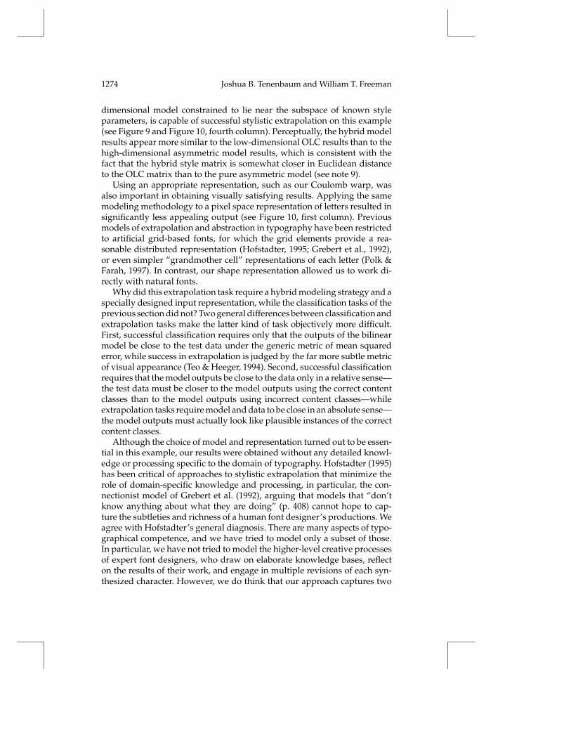
1274 Joshua B. Tenenbaum and William T. Freeman
dimensional model constrained to lie near the subspace of known styleparameters, is capable of successful stylistic extrapolation on this example(see Figure 9 and Figure 10, fourth column). Perceptually, the hybrid modelresults appear more similar to the low-dimensional OLC results than to thehigh-dimensional asymmetric model results, which is consistent with thefact that the hybrid style matrix is somewhat closer in Euclidean distanceto the OLC matrix than to the pure asymmetric model (see note 9).
Using an appropriate representation, such as our Coulomb warp, wasalso important in obtaining visually satisfying results. Applying the samemodeling methodology to a pixel space representation of letters resulted insignificantly less appealing output (see Figure 10, first column). Previousmodels of extrapolation and abstraction in typography have been restrictedto artificial grid-based fonts, for which the grid elements provide a rea-sonable distributed representation (Hofstadter, 1995; Grebert et al., 1992),or even simpler “grandmother cell” representations of each letter (Polk &Farah, 1997). In contrast, our shape representation allowed us to work di-rectly with natural fonts.
Why did this extrapolation task require a hybrid modeling strategy and aspecially designed input representation, while the classification tasks of theprevious section did not? Two general differences between classification andextrapolation tasks make the latter kind of task objectively more difficult.First, successful classification requires only that the outputs of the bilinearmodel be close to the test data under the generic metric of mean squarederror, while success in extrapolation is judged by the far more subtle metricof visual appearance (Teo & Heeger, 1994). Second, successful classificationrequires that the model outputs be close to the data only in a relative sense—the test data must be closer to the model outputs using the correct contentclasses than to the model outputs using incorrect content classes—whileextrapolation tasks require model and data to be close in an absolute sense—the model outputs must actually look like plausible instances of the correctcontent classes.
Although the choice of model and representation turned out to be essen-tial in this example, our results were obtained without any detailed knowl-edge or processing specific to the domain of typography. Hofstadter (1995)has been critical of approaches to stylistic extrapolation that minimize therole of domain-specific knowledge and processing, in particular, the con-nectionist model of Grebert et al. (1992), arguing that models that “don’tknow anything about what they are doing” (p. 408) cannot hope to cap-ture the subtleties and richness of a human font designer’s productions. Weagree with Hofstadter’s general diagnosis. There are many aspects of typo-graphical competence, and we have tried to model only a subset of those.In particular, we have not tried to model the higher-level creative processesof expert font designers, who draw on elaborate knowledge bases, reflecton the results of their work, and engage in multiple revisions of each syn-thesized character. However, we do think that our approach captures two

Separating Style and Content 1275
essential aspects of the human competence in font extrapolation: people’srepresentations of letter and font characteristics are modular and indepen-dent of each other, and people’s knowledge of letters and fonts is abstractedfrom the ability to perform the particular task of character synthesis. Genericconnectionist approaches to font extrapolation such as Grebert et al. (1992)do not satisfy these constraints. Letter and font information is mixed to-gether inextricably in the extrapolation network’s weights, and an entirelydifferent network would be needed to perform recognition or classificationtasks with the same stimuli. Our bilinear modeling approach, in contrast,captures the perceptual modularity of style and content in terms of the math-ematical property of separability that characterizes equations 2.1 through2.7. Knowledge of style s (in equation 2.6, for example) is localized to thematrix parameter As, while knowledge of content class c is localized to thevector parameter bc, and both can be freely combined with other contentor style parameters, respectively. Moreover, during training, our modelsacquire knowledge about the interaction of style and content factors thatis truly abstracted from any particular behavior, and thus can support notonly extrapolation of a novel style, but also a range of other synthesis andrecognition tasks as shown in Figure 1.
6 Translation
Many important perceptual tasks require the perceiver to recover simul-taneously two unknown pieces of information from a single stimulus inwhich these variables are confounded. A canonical example is the problemof separating the intrinsic shape and texture characteristics of a face fromthe extrinsic lighting conditions, which are confounded in any one imageof that face. In this section, we show how a perceptual system may, usinga bilinear model, learn to solve this problem from a training set of faceslabeled according to identity and lighting condition. The bilinear model al-lows a novel face viewed under a novel illuminant to be translated to itsappearance under known lighting conditions, and the known faces to betranslated to the new lighting condition. Such translation tasks are the mostdifficult kind of two-factor learning task, because they require generaliza-tion across both factors at once. That is, what is common across both trainingand test data sets is not any particular style or any particular content class,but only the manner in which these two factors interact. Thus, only a sym-metric bilinear model (see equations 2.1–2.3) is appropriate, because onlyit represents explicitly the interaction between style and content factors, inthe Wk parameters.
6.1 Task Specifics. Given a training set of S = 23 faces (content) viewedunder C = 3 different lighting conditions (style) and a novel face viewedunder a novel light source, the task is to translate the new face to knownlighting conditions and the known faces to the new lighting condition. The

1276 Joshua B. Tenenbaum and William T. Freeman
face images, provided by Y. Moses of the Weizmann Institute, were croppedto remove nonfacial features and blurred and subsampled to 48× 80 pixels.Because these faces were aligned and lacked sharp edge features (unlikethe typographical characters of the previous section), we could representthe images directly as 3840-dimensional vectors of pixel brightness values.
6.2 Algorithm. We first fit the symmetric model (see equation 2.2) tothe training data using the iterated SVD procedure described in section 3.2.This yields vector representations as and bc of each face c and illuminants, and a matrix of interaction parameters W (defined in equation 3.8). Thedimensionalities for as and bc were set equal to S and C, respectively, allow-ing the bilinear model maximum expressivity while still ensuring a uniquesolution. Because these dimensionalities were set to their maximal values,only one iteration of the fitting algorithm (taking approximately 10 seconds)was required for complete training.
For generalization from a single test image y, we adapt the model si-multaneously to both the new face identity c and the new illuminant s,while holding fixed the face × illuminant interaction term W learned dur-ing training. Specifically, we first make an initial guess for the new faceidentity vector bc (e.g., the mean of the training set style vectors) and solvefor the least-squares optimal estimate of the illuminant vector as:
as =[[
Wbc]VT
]−1
y. (6.1)
Here [. . .]−1 denotes the pseudoinverse function. Given this new value foras, we then reestimate bc from
bc =[[
WVTas]VT
]−1
y, (6.2)
and iterate equations 6.1 and 6.2 until both as and bc converge. In the ex-ample presented in Figure 11, convergence occurred after 14 iterations (ap-proximately 16 seconds). We can then generate images of the new face underknown illuminant s (from ysc
k = asTWkbc) and of known face c under the new
illuminant (from ysck = asT
Wkbc).
6.3 Results. Figure 11 shows results, with both the old faces translatedto the new illuminant and the new face translated to the old illuminants. Forcomparison, the true images are shown next to the synthetic ones. Again,evaluation of these results must necessarily be subjective. The lighting andshadows for each synthesized image appear approximately correct, as dothe facial features of the old faces translated to the new illuminant. The fa-cial features of the new face translated to the old illuminants appear slightly

Separating Style and Content 1277
? ?
?
?
synthetic
actual
A B
C
Figure 11: Translation across style and content in shape-from-shading. (A) Row1–3: The first 13 (of 24) faces viewed under the three illuminants used for training.Row 4: The single test image of a new face viewed under a new light source.(B) Column 1: Translation of the new face to known illuminants. Column 2:The actual (unseen) images. (C) Row 1: Translation of known faces to the newilluminant. Row 2: The actual (unseen) images.
blurred, but otherwise resemble the new face more than any of the old faces.One reason the synthesized images of the new face are not as sharp as thesynthesized images of the old faces is that the latter are produced by averag-ing images of a single face under several lighting conditions—across whichall the facial features are precisely aligned—while the former are producedby averaging images of many faces under a single lighting condition—acrosswhich the facial features vary significantly in their positions.
6.4 Discussion. A history of applying linear models to face images mo-tivates our bilinear modeling approach. The original work on eigenfaces(Kirby & Sirovich, 1990; Turk & Pentland, 1991) showed that images ofmany different faces taken under fixed lighting and viewpoint conditionsoccupy a low-dimensional linear subspace of pixel space. Subsequent workby Hallinan (1994) established the complementary result that images of asingle face taken under many different lighting conditions also occupy alow-dimensional linear subspace. Thus, the factors of facial identity andillumination have already been shown to satisfy approximately the defini-tion of bilinearity—the effects of one factor are linear when the other is heldconstant—so it is natural to integrate them into a bilinear model.
1278 Joshua B. Tenenbaum and William T. Freeman
While the general problem of separating shape, texture, and illumina-tion features in an image is underdetermined (Barrow & Tenenbaum, 1978),here the bilinear model learned during training provides sufficient con-straint to approximately recover both face and illumination parametersfrom a single novel image. Atick, Griffin, & Redlich (1996) proposed a re-lated approach to learning shape-from-shading for face images, based ona linear model of head shape in three dimensions and a nonlinear physi-cal model of the image formation process. In contrast, our bilinear modeluses only two-dimensional (i.e., image-based) information and requires noprior knowledge about the physics of image formation. Of course, we havenot solved the general shape-from-shading recovery problem for arbitraryobjects under arbitrary illumination. Our solution (as well as that of At-ick et al., 1996) depends critically on the assumption that the new image,like the images in the training set, depicts an upright face under reasonablelighting conditions. In fact, there is evidence that the brain often does notsolve the shape-from-shading problem in its most general form, but ratherhas learned (or evolved) solutions to important special cases such as faceimages (Cavanagh, 1991). So-called Mooney faces—brightness-thresholdedface images in which shading is the only cue to shape—can be easily rec-ognized as images of three-dimensional surfaces when viewed in uprightposition, but cannot be discriminated from two-dimensional ink blotcheswhen viewed upside down so that the shading conventions are atypical(Shepard, 1990), or when the underlying three-dimensional structure hasbeen distorted away from a globally facelike shape (Moore & Cavanagh,1998). More generally, the ability to learn constrained solutions to a prioriunderconstrained inference problems may turn out to be essential for per-ception (Poggio & Hurlbert, 1994; Nayar & Poggio, 1996). Bilinear modelsoffer one simple and general framework for how biological and artificialperceptual systems may learn to solve a wide range of such tasks.
7 Directions for Future Work
The most obvious extension of our work is to observations and tasks withmore than two underlying factors, via multilinear models (Magnus & Neu-decker, 1988). For example, a symmetric trilinear model in three factors q, r,and s would take the form:
yqrsl =
∑i,j,k
wijklaqi br
j csk. (7.1)
The procedures for fitting these models are direct generalizations of thelearning algorithms for two-factor models that we describe here. As in thetwo-factor case, we iteratively apply linear matrix techniques to solve for theparameters of each factor given parameter estimates for the other factors,until all parameter estimates converge (Magnus & Neudecker, 1988).
Separating Style and Content 1279
As with any other learning framework, the success of bilinear models de-pends on having suitable input representations. Further research is neededto determine what kinds of representations will endow specific kinds ofobservations with the most nearly bilinear structure. In particular, the fontextrapolation task might benefit from a representation that is better tai-lored to the important features of letter shapes. Also, it would be of interestto develop general procedures for incorporating available domain-specificknowledge into bilinear models, for example, via a priori constraints on themodel parameters (Simard, LeCun, & Denker, 1993).
Finally, we would like to explore the relevance of bilinear models forresearch in neuroscience and psychophysics. The essential representationalfeature of bilinear models is their multiplicative factor interactions. At thephysiological level, multiplicative neuronal interactions (Andersen, Essick,& Siegel, 1985; Olshausen, Anderson, & van Essen, 1993; Riesenhuber &Dayan, 1997), arising from nonlinear synaptic (Koch, 1997) or population-level (Salinas & Abbott, 1993) mechanisms, have been proposed for visualcomputations that require the synergistic combination of two inputs, suchas modulating spatial attention (Andersen et al., 1985; Olshausen et al.,1993; Riesenhuber & Dayan, 1997; Salinas & Abbott, 1993) or estimatingmotion (Koch, 1997). May these same kinds of circuits be co-opted to per-form some of the tasks we study here? It has been suggested that SVD, theessential computational procedure for learning in our framework, can beimplemented naturally in neural networks using Hebb-like learning rules(Sanger, 1989, 1994; Oja, 1989). Could these or similar mechanisms supporta biologically plausible learning algorithm for bilinear models? At the levelof psychophysics, many studies have demonstrated that the ability of thehuman visual and auditory systems to factor out contextually irrelevantdimensions of variation, such as lighting conditions or speaker accent, isneither perfect nor instantaneous. Observations in unusual styles are fre-quently more time-consuming to process and more likely to be processedincorrectly (van Bergem et al., 1988; Sanocki, 1992; Nygaard & Pisoni, 1998;Moore & Cavanagh, 1998). Do bilinear models have difficulty on the samekinds of stimuli that people do? Do the dynamics of adaptation in bilinearmodels (e.g., EM for classification, or the iterative SVD-based procedure fortranslation) take longer to converge on stimuli that people are slower toprocess? Can our approach provide a framework for designing and mod-eling perceptual learning experiments, in which subjects learn to separatethe effects of style and content factors in a novel stimulus domain? Theseare just a few of the empirical questions motivated by a bilinear modelingapproach to studying perceptual inference.
8 Conclusions
In one sense, bilinear models are not new to perceptual research. It has pre-viously been shown that several core vision problems, such as the recovery
1280 Joshua B. Tenenbaum and William T. Freeman
of structure from motion under orthographic projection (Tomasi & Kanade,1992) and color constancy under multiple illuminants (Brainard & Wandell,1991; Marimont & Wandell, 1992; D’Zmura, 1992) are solvable efficientlybecause they are fundamentally bilinear at the level of geometry or physics(Koenderink & van Doorn, 1997). These results are important but of limitedusefulness, because many two-factor problems in perception do not havethis true bilinear character. More commonly, perceptual inferences basedon accurate physical models of factor interactions are either very complex(as in speech recognition), underdetermined (as in shape-from-shading), orsimply inappropriate (as in typography).
Here we have proposed that perceptual systems may often solve suchchallenging two-factor tasks without detailed domain knowledge, using bi-linear models to learn approximate solutions rather than to describe explic-itly the intrinsic geometry or physics of the problem. We presented a suiteof simple and efficient learning algorithms for bilinear models, based onthe familiar techniques of SVD and EM. We then demonstrated the scope ofthis approach with applications to three two-factor tasks—classsification,extrapolation, and translation—using three kinds of signals—speech, ty-pography, and face images. With their combination of broad applicabilityand ready learning algorithms, bilinear models may prove to be a generallyuseful component in the tool kits of engineers and brains alike.
Acknowledgments
We thank E. Adelson, B. Anderson, M. Bernstein, D. Brainard, P. Dayan, W.Richards, and Y. Weiss for helpful discussions. Joshua Tenenbaum was aHoward Hughes Medical Institute predoctoral fellow. Preliminary reportsof this material appeared in Tenenbaum and Freeman (1997) and Freemanand Tenenbaum (1997).
References
Andersen, R., Essick, G., & Siegel, R. (1985). The encoding of spatial location byposterior parietal neurons. Science, 230, 456–458.
Atick, J. J., Griffin, P. A., & Redlich, A. N. (1996). Statistical approach to shapefrom shading: Reconstruction of 3d face surfaces from single 2d images.Neural Computation, 8, 1321–1340.
Barrow, H. G., & Tenenbaum, J. M. (1978). Recovering intrinsic scene character-istics from images. In A. R. Hanson & E. M. Riseman (Eds.), Computer visionsystems (pp. 3–26). New York: Academic Press.
Bell, A., & Sejnowski, T. (1995). An information–maximization approach toblind separation and blind deconvolution. Neural Computation, 7(6), 1129–1159.
Beymer, D., & Poggio, T. (1996). Image representations for visual learning. Sci-ence, 272, 1905–1909.
Separating Style and Content 1281
Bishop, C. M. (1995). Neural networks for pattern recognition. New York: OxfordUniversity Press.
Brainard, D., & Wandell, B. (1991). A bilinear model of the illuminant’s effecton color appearance. In M. S. Landy and J. A. Movshon (Eds.), Computationalmodels of visual processing (chap. 13). Cambridge, MA: MIT Press.
Caruana, R. (1998). Multitask learning. In S. Thrun and L. Pratt (Eds.), Learningto learn (pp. 95–134). Norwell, MA: Kluwer.
Cavanagh, P. (1991). What’s up in top-down processing? In A. Gorea (Ed.),Representations of vision: Trends and tacit assumptions in vision research (pp. 295–304). Cambridge: Cambridge University Press.
Dayan, P., Hinton, G., Neal, R., & Zemel, R. (1995). The Helmholtz machine.Neural Computation, 7(5), 889–904.
Dempster, A. P., Laird, N. M., & Rubin, D. B. (1977). Maximum likelihood fromincomplete data via the EM algorithm. Journal of Royal Statist. Soc. B, 39,1–38.
Duda, R. O., & Hart, P. E. (1973). Pattern classification and scene analysis. NewYork: Wiley-Interscience.
D’Zmura, M. (1992). Color constancy: Surface color from changing illumination.Journal of the Optical Society of America A, 9, 490–493.
Freeman, W. T., & Tenenbaum, J. B. (1997). Learning bilinear models for two-factor problems in vision. In Proc. IEEE Conference on Computer Vision andPattern Recognition (pp. 554–560). San Juan, PR.
Ghahramani, Z. (1995). Factorial learning and the EM algorithm. In G. Tesauro,D. Touretzky, and T. Leen (Eds.), Advances in neural information processingsystems (Vol. 7, pp. 617–624). Cambridge, MA: MIT Press.
Grebert, I., Stork, D. G., Keesing, R., & Mims, S. (1992). Connectionist general-ization for production: An example from gridfont. Neural Networks, 5, 699–710.
Hallinan, P. W. (1994). A low-dimensional representation of human faces forarbitrary lighting conditions. In Proc. IEEE Conference on Computer Vision andPattern Recognition (pp. 995–999).
Hastie, T., & Tibshirani, R. (1996). Discriminant adaptive nearest neighbor clas-sification. IEEE Transactions on Pattern Analysis and Machine Intelligence, 18,607–616.
Hinton, G., Dayan, P., Frey, B., & Neal, R. (1995). The wake-sleep algorithm forunsupervised neural networks. Science, 268, 1158–1161.
Hinton, G., & Ghahramani, Z. (1997). Generative models for discovering sparsedistributed representations. Phil. Trans. Royal Soc. B, 352, 1177–1190.
Hinton, G. E., & Zemel, R. (1994). Autoencoders, minimum description length,and Helmholtz free energy. In J. Cowan, G. Tesauro, and J. Alspector (Eds.),Advances in neural information processing systems, 6 (pp. 3–10). San Mateo, CA:Morgan Kauffman.
Hofstadter, D. (1985). Metamagical themas. New York: Basic Books.Hofstadter, D. (1995). Fluid concepts and creative analogies. New York: Basic Books.Holyoak, K., & Barnden, J. (Eds.). (1994). Advances in connectionist and neural
computation theory. Norwood, NJ: Ablex.Jackson, J. D. (Ed.). (1975). Classical electrodynamics (2nd ed.). New York: Wiley.
1282 Joshua B. Tenenbaum and William T. Freeman
Kirby, M., & Sirovich, L. (1990). Application of the Karhunen-Loeve procedurefor the characterization of human faces. IEEE Transactions on Pattern Analysisand Machine Intelligence, 12(1), 103–108.
Koch, C. (1997). Computation and the single neuron. Nature, 385, 207–211.Koenderink, J. J., & van Doorn, A. J. (1997). The generic bilinear calibration–
estimation problem. International Journal of Computer Vision, 23(3), 217–234.Magnus, J. R., & Neudecker, H. (1988). Matrix differential calculus with applications
in statistics and econometrics. New York: Wiley.Mardia, K., Kent, J., & Bibby, J. (1979). Multivariate analysis. London: Academic
Press.Marimont, D. H., & Wandell, B. A. (1992). Linear models of surface and illumi-
nant spectra. Journal of the Optical Society of America A, 9(11), 1905–1913.Moghaddam, B., & Pentland, A. P. (1997). Probabilistic visual learning for object
representation. IEEE Transactions on Pattern Analysis and Machine Intelligence,19(7), 696–710.
Moore, C., & Cavanagh, P. (1998). Recovery of 3d volume from 2-tone imagesof novel objects. Cognition, 67 (1,2), 45–71.
Nayar, S., & Poggio, T. (Eds.). (1996). Early visual learning. New York: OxfordUniversity Press.
Nygaard, L. C., & Pisoni, D. B. (1998). Talker-specific learning in speech percep-tion. Perception and Psychophysics, 60(3), 355–376.
Oja, E. (1989). Neural networks, principal components, and subspaces. Interna-tional Journal of Neural Systems, 1, 61–68.
Olshausen, B., Anderson, C., & van Essen, D. (1993). A neural model of visualattention and invariant pattern recognition. Journal of Neuroscience, 13, 4700–4719.
Omohundro, S. M. (1995). Family discovery. In D. Touretzky, M. Moser, & M.Hasselmo (Eds.), Advances in neural information processing systems, 8 (pp. 402–408). Cambridge, MA: MIT Press.
Poggio, T., & Hurlbert, A. (1994). Observations on cortical mechanisms for objectrecognition and learning. In C. Koch & J. Davis (Eds.), Large scale neuronaltheories of the brain (pp. 152–182). Cambridge, MA: MIT Press.
Polk, T. A., & Farah, M. J. (1997). A simple common contexts explanation for thedevelopment of abstract letter identities. Neural Computation, 9(6), 1277–1289.
Press, W. H., Teukolsky, S. A., Vetterling, W. T., & Flannery, B. P. (1992). Numericalrecipes in C. New York: Cambridge University Press.
Riesenhuber, M., & Dayan, P. (1997). Neural models for part-whole hierarchies.In M. Mozer, M. Jordan, & T. Petsche (Eds.), Advances in neural informationprocessing systems, 9 (pp. 17–23). Cambridge, MA: MIT Press.
Robinson, A. (1989). Dynamic error propagation networks. Unpublished doctoraldissertation, Cambridge University.
Salinas, E., & Abbott, L. (1993). A model of multiplicative neural responses inparietal cortex. In Proc. Nat. Acad. Sci. USA (pp. 11956–11961).
Sanger, T. D. (1989). Optimal unsupervised learning in a single-layer linear feed-forward neural network. Neural Networks, 2, 459–473.
Sanger, T. (1994). Two algorithms for iterative computation of the singularvalue decomposition from input/output samples. In J. Cowan, G. Tesauro, &
Separating Style and Content 1283
J. Alspector (Eds.), Advances in neural information processing systems, 6 (pp. 144–151). San Mateo, CA: Morgan Kauffman.
Sanocki, T. (1992). Effects of font- and letter-specific experience on the perceptualprocessing of letters. American Journal of Psychology, 105(3), 435–458.
Shepard, R. N. (1990). Mind sights. New York: Freeman.Simard, P. Y., LeCun, Y., & Denker, J. (1993). Efficient pattern recognition using
a new transformation distance. In S. Hanson, J. Cowan, & L. Giles (Eds.),Advances in neural information processing systems, 5. San Mateo, CA: MorganKaufman.
Szeliski, R., & Tonnesen, D. (1992). Surface modeling with oriented particlesystems. In Proc. SIGGRAPH 92 (Vol. 26, pp. 185–194).
Tenenbaum, J. B., & Freeman, W. T. (1997). Separating style and content. InM. Mozer, M. Jordan, & T. Petsche (Eds.), Advances in neural information pro-cessing systems, 9 (pp. 662–668). Cambridge, MA: MIT Press.
Teo, P., & Heeger, D. (1994). Perceptual image distortion. In First IEEE Interna-tional Conference on Image Processing (Vol. 2, pp. 982–986). New York: IEEE.
Thrun, S., & Pratt, L. (Eds). (1998). Learning to learn. Norwell, MA: Kluwer.Tomasi, C., & Kanade, T. (1992). Shape and motion from image streams under
orthography: A factorization method. International Journal of Computer Vision,9(2), 137–154.
Turk, M., & Pentland, A. (1991). Eigenfaces for recognition. Journal of CognitiveNeuroscience, 3(1), 71–86.
van Bergem, D. R., Pols, L. C., & van Beinum, F. J. K. (1988). Perceptual nor-malization of the vowels of a man and a child in various contexts. SpeechCommunication, 7(1), 1–20.
Received October 27, 1998; accepted June 8, 1999.