Sensors, Transducers and TransmittersThe definition of a sensor, a transducer, and a transmitter has been a topic of debate since at least the late 1980's. The problems with specific definitions become one of semantics. These devices were defined in the introduction, but rather than entering the debate, let's use the following definitions for these terms for purposes of this module.

●Sensor – A device that responds to [a] stimulus and provides a measurable output but does not provide any processing of that output

●Transducer – A sensor on a mount with some basic signal processing to get uncalibrated mV or other signal. The signal processing is generally a conversion from one signal form to another.

●Transmitter – Sensor on a mount with signal processing to get calibrated output to a standard output range such as 2-10 Vdc, 4-20 mA, 3-15 psi, etc.

A couple of examples are in order. Consider the pneumatic temperature transmitter shown in Figure 1. This unit is comprised of a brass tube that is inserted into the fluid of which temperature we wish to measure. As the brass tube changes temperature, it also changes length. The brass tube can be considered the sensing element. Within the tube is a rod, which is attached at the other end to a flap. This flap works against a spring to cover an air port. As the brass tube (sensing element) changes length, the rod/flap assembly acts as a valve to allow more or less air to flow through the port. This is the transducer portion of the unit. It converts one signal, the change in length of the brass tube, into another, a pneumatic signal. The entire unit can be considered a transmitter. As defined above the transmitter assembly is comprised of a sensor (brass tube) with signal processing (the opening/closing of the air valve) to output a standard pneumatic signal to the controller of 3-15 psi over its sensing range.

On the other hand, Figures 3, 4 and 5 represent electronic temperature detection through the use of an RTD (Resistance Temperature Detector). The RTD device is one that changes resistance with a change in temperature. It constitutes the sensor. The resistance of the RTD is measured and converted to an electrical current or voltage by

Figure 1 Pneumatic Type Temperature Transmitter

means of a Wheatstone bridge. The Wheatstone bridge would constitute the transducer. The signal from the transducer is converted to a standard 4-20 ma output. The entire assembly can be considered a temperature transmitter. However, in practice, the electronic board to which the sensor is attached is usually referred to as the transmitter.

As you can see, the terminology is rather arbitrary and very semantic. In the example above, one could consider the RTD a transducer since it converts heat intensity into an electrical resistance. Although such semantic differentiation is probably quite important to some, it is not critical for our purposes. For our discussions, we will use the definitions outlined above.

Single Variable vs. Multi-variable Sensing

Measurement sensing can be classified as mechanical, electrical or analytical. Common mechanical measurements include pressure, temperature, humidity, flow rate, liquid level, force, velocity, acceleration, and position to name but a few. Electrical measurements are generally voltage, resistance and current, but can also include capacitance, inductance, charge, etc. Measurements of analytical properties may include electrical conductivity, thermal conductivity, chromatography, turbidity, density, pH, etc. As one may surmise, if a property exists it can probably be measured.

Single variable sensing is debatably the most common. Just as it sounds, we are sensing the value of a single property of a body or substance. It is important to note most measurements cannot be taken directly. For example, temperature is a measurement of heat intensity; which, in turn, is directly related to the average velocity of the molecules comprising the substance being measured. Obviously, the direct measurement of molecular velocity is not practical; we must find a different way to measure temperature. To that end, the pneumatic temperature transmitter described above is designed based upon a well-known relationship between temperature and the thermal expansion of brass. Thus, this unit provides temperature indication by measuring the change in length of the brass tube. This change in length is converted to an air pressure as described above.

Another example of indirect measurement is that of fluid flow. One of the most common methods of measuring fluid flow is to detect the pressure difference across a restriction. This differential pressure has a direct relationship to volume flow rate by means of a mathematical equation developed by the manufacturer of the device.

Multi-variable sensing is used to provide information regarding properties that also cannot be measured directly. For example, we may wish to measure the heat flow rate in a reboiler for purposes of controlling the flow of steam to a distillation column. From a course in thermodynamics, we know that heat flow is defined as:

( )2 1pq m xc x T T= −&

where:

2

1

p

q heat flowrate

m mass flowrate

c specific heat

T outlet temperature

T inlet temperature

===

=

=

&

The specific heat is a material property that can usually be considered a constant. If it does vary widely with temperature, this variation is predictable and can also be mathematically defined. If we measure both temperatures and the mass flow rate of fluid, we can send this information to a central processor. The processor is programmed with the above equation(s) to provide the controller a value representing heat flow rate. The controller then responds to this value based on its tuning parameters.

Types of Sensors

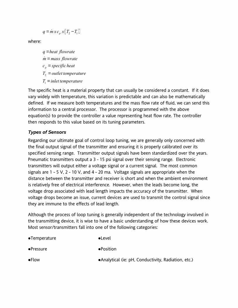
Regarding our ultimate goal of control loop tuning, we are generally only concerned with the final output signal of the transmitter and ensuring it is properly calibrated over its specified sensing range. Transmitter output signals have been standardized over the years. Pneumatic transmitters output a 3 - 15 psi signal over their sensing range. Electronic transmitters will output either a voltage signal or a current signal. The most common signals are 1 - 5 V, 2 - 10 V, and 4 - 20 ma. Voltage signals are appropriate when the distance between the transmitter and receiver is short and when the ambient environment is relatively free of electrical interference. However, when the leads become long, the voltage drop associated with lead length impacts the accuracy of the transmitter. When voltage drops become an issue, current devices are used to transmit the control signal since they are immune to the effects of lead length.

Although the process of loop tuning is generally independent of the technology involved in the transmitting device, it is wise to have a basic understanding of how these devices work. Most sensor/transmitters fall into one of the following categories:

●Temperature

●Pressure

●Flow

●Level

●Position

●Analytical (ie: pH, Conductivity, Radiation, etc.)

Temperature Sensors

Electronic temperature sensors come in two basic varieties: resistance devices and voltage devices. A resistance device is one in which the resistance varies with temperature. Resistance devices can be further classified as a PTC (Positive Temperature Coefficient) device, or an NTC (Negative Temperature Coefficient) device. The resistance of a PTC increases with an increase in temperature; the most common being the RTD. Conversely, the resistance of an NTC decreases with an increase in temperature. The most common NTC is a thermistor.

The RTD is a very stable, highly accurate and very precise. It exhibits nearly linear characteristics. These characteristics allow for very simple replacement of a damaged RTD without having to retune the control loop. The characteristic of a typical RTD is shown as a graph in Figure 2. Note the linearity. An RTD may be constructed of 1000 ohm platinum wire (or film), a 100 ohm platinum wire (or film), nickel-iron (balco), or copper. Except for the 1000 ohm unit, all sensors must be used with a transmitter. Although the use of a transmitter on 1000 ohm units is common, it is not required. RTD's are available as two-wire, three-wire, or four-wire devices. The basic device used to measure the resistance of the RTD is a Wheatstone bridge. As depicted in Figure 3, the basic device only requires two-wires in order to provide a signal to a transducer. However, if the leads are very long,

--25 0 25 50 75 100 125 150 175 200 225 250

600

800

1000

1200

1400

1600

1800

Johnson ControlsTypical RTD Performance

1,000 Ohm at 70 FRange: -40 to 250 F

Temperature

Res

ista

nce

Figure 2 Typical RTD characteristics

S i g n a lP o w e r

R T D

T r a n s m i t t e r

Figure 4 Four-Wire RTD

Figure 3: Two-wire RTD

S i g n a lP o w e r a n d T r a n s d u c e r

C i r c u i t sR T D

T r a n s m i t t e r

S i g n a lP o w e r a n d T r a n s d u c e r

C i r c u i t sR T D

T r a n s m i t t e r

Figure 5 Three-Wire RTD

wire resistance becomes a large percentage of the measured resistance and introduces significant error. Typically, we can compensate for this by using a three-wire RTD. The three-wire RTD is connected as shown in Figure 4. In this arrangement, the two outer wires are of the same length and necessarily connected on opposing terminals of the Wheatstone bridge. This allows effects of lead resistance to cancel. The third wire is used to carry the actual signal. Since the signal is a current measured in terms of micro-amps, the error inherent in the two-wire RTD is nearly eliminated.

A four wire RTD is used where high degree of accuracy is required. However, the transducer/transmitter assembly is quite different. Instead of using a Wheatstone bridge, a four-wire RTD is connected across a power supply and some form of voltage meter. This is illustrated in Figure 5. The advantage of this arrangement is the ability to read the voltage drop across the RTD for any given temperature. As long as the lead wires are of the same length, this voltage drop is not affected by line length. Since we know the temperature sensed by an RTD is proportional to the resistance of the RTD, and since we know resistance is directly related to voltage drop, we can relate temperature directly to voltage drop in a very accurate manner.

There are several downsides to an RTD. First, if local indication is required, one will need to either install a mechanical thermometer or will have to retransmit the temperature signal back to an electronic indicator. Second, a voltage must be provided to induce a current so that resistance can be measured. We may also remember that electrical power is defined as P = I2 R. This generates heat. The accuracy of the RTD can be subject to self-heating effects.

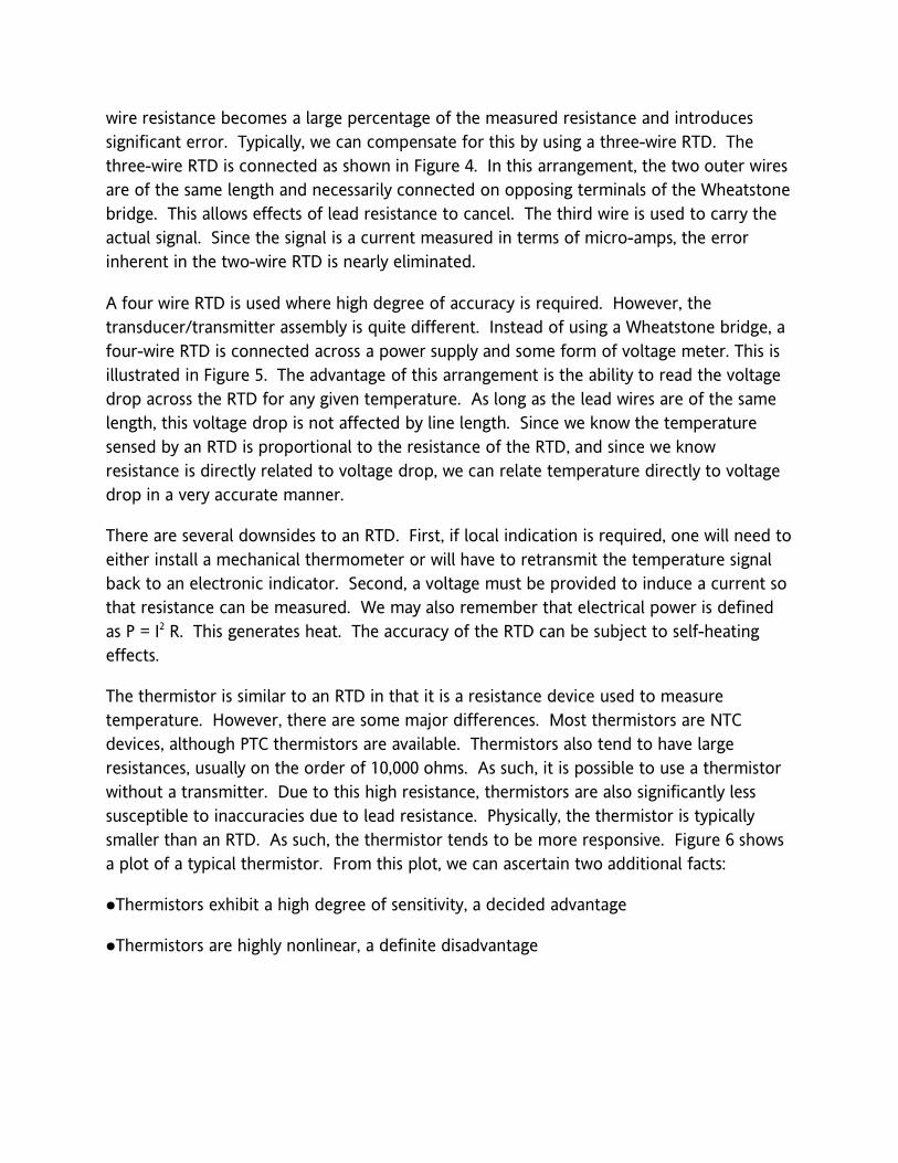
The thermistor is similar to an RTD in that it is a resistance device used to measure temperature. However, there are some major differences. Most thermistors are NTC devices, although PTC thermistors are available. Thermistors also tend to have large resistances, usually on the order of 10,000 ohms. As such, it is possible to use a thermistor without a transmitter. Due to this high resistance, thermistors are also significantly less susceptible to inaccuracies due to lead resistance. Physically, the thermistor is typically smaller than an RTD. As such, the thermistor tends to be more responsive. Figure 6 shows a plot of a typical thermistor. From this plot, we can ascertain two additional facts:

●Thermistors exhibit a high degree of sensitivity, a decided advantage

●Thermistors are highly nonlinear, a definite disadvantage

The responsiveness, the sensitivity, and the low susceptibility to lead resistance make thermistors a popular choice of temperature sensor. The lack of nonlinearity does pose some special problems, but is rather easily handled through the use of a characterizer to linearize the output. Other disadvantages include the same difficulties with local indication and self-heating as described above for the RTD.

-25 0 25 50 75 100 125 150 175 200 225

0

20

40

60

80

100

120

140

160

Kreuter STE-1254Thermistor Element10,000 Ohm at 77 FRange: -30 to 240 F

Temperature

Res

ista

nce

(100

0 o

hms)

Figure 6 Typical Thermistor Characteristics

R e c e i v e r

C o l d J u n c t i o n C o m p e n s a t i o n

C u

C

C u

C u

T y p e T

Figure 7 Type T Thermocouple Circuit

The thermocouple is an example of a voltage device. When two wires of differing materials are joined at one end, and that end is subjected to a heat flux, one is able to measure a voltage potential across the open ends. This potential is referred to as Seebeck voltage in honor of the scientist who made this discovery. A type 'T' thermocouple circuit is illustrated in Figure 7. Type 'T' thermocouples are comprised of one copper wire and one constantan wire. Notice one junction is connected to a cold junction compensation circuit.

When using a thermocouple, the temperature of one junction must be known. One such method would be to immerse a junction into an ice bath, thus keeping the junction at 32 oF. This is impractical in the field. In lieu of an ice bath, we use some form of temperature compensation circuit. Typically, this circuit is nothing more than another temperature sensor such as a thermistor. It could also be a thermoelectric heater or cooler designed to hold this junction at some design temperature. In either case, the temperature is known and the voltage induced at this connection is constant. When a heat flux is applied to the sensing junction, the receiver detects millivoltage, which is directly related to the temperature at the sensing junction. The characteristics of a Type T thermocouple are shown in Figure 8.

-150 -100 -50 0 50 100 150 200 250 300 350 400 450 500 550 600 650 700

-10

-5

0

5

10

15

20

25

30

35

40

Type T Thermocouple

Temperature (Degrees C)

Vol

tage

(m

illiv

olts

)

Figure 8 Response of a Type T Thermocouple at a 0 C reference

As with the RTD and thermistor, thermocouples have their advantages and disadvantages. The primary advantages of a thermocouple are the simplicity of construction, the rugged nature of the device, and the wide range of temperatures. As indicated in Figure 7, the Type T thermocouple has a sensing range of -150 C to 700 C (-240 F to 1300 F). Thermocouples are less prone to failure due to vibration and can also be mechanically clamped, even welded, to the unit in which temperature is being sensed. The material from which thermocouple wire is manufactured is quite varied. Each thermocouple is assigned a type letter and a useful application range. Table 1 lists some of the more popular thermocouples available.

Thermocouple wire insulation and the outer jacket is also color-coded. Unfortunately, there is no global standard for color-coding. Some common standards are the US ASTM, British BS1843-1952, British BS4937-Part 30-1993, French NFE and German DIN standards. Figure 9 indicates the color standard described under the US ASTM guidelines. It is important one understand and double-check color coding, especially if you work with European suppliers. Catastrophic industrial incidents have been recorded where the cause

Type Wire Material (+ / -) Range

B Platinum/6% Rhodium – Platinum/30%Rhodium 2500 -3100 F

C W5Re Tungsten/5% Rhodium – W26Re Tungsten/26% Rhodium 3000 – 4200 F

E Chromel – Constantan 200 to 1650 F

J Iron – Constantan 200 – 1400 F

K Chromel – Alumel 200 – 2300 F

N Nicrosil - Nisil 1200 – 2300 F

R Platinum/13% Rhodium - Platinum 1600 – 2640 F

S Platinum/10% Rhodium - Platinum 1800 – 2640 F

T Copper – Constantan -330 – 660 F

Table 1 Thermocouple Types and Application Ranges

of the accident was traced back to misinterpretation of color-coding on thermocouple wiring.

Pressure Transmitters

Pressure is one of the most common properties to detect. We frequently sense differential pressure to determine fluid flow, liquid level, and equipment performance. Pressure transmitters can be designed to measure absolute pressure or gage pressure. All sensors will sense pressure above atmospheric. Most, but not all, will measure pressure below

Type Vacuum Range Pressure Range Typical Accuracy Additional Errors

Strain gage 1 mm Hga to -10 in w.g. +3 in w.g. to 106 psi 0.1% span to 0.3% FSO 0.25% FSO Drift over 6 months0.25% FSO per 1000 F

Capacitive 300 mm Hga to -1 in w.g +5 in w.g. to 104 psi 0.1% reading or 0.01% FSO

0.25% FSO per 1000 F

Potentiometric -200 in w.g. To -1 in w.g. +5 in w.g. To 104 psi 0.5% to 1.0% FSO Subject to mechanical wear and temperature drift

Vibrating Wire 1 mm Hg to -2 in w.g. +5 in w.g. to 104 psi 0.1% span 0.1% span over 6 months0.2% span per 1000 F

Piezoelectric N/A +10 in w.g. to 104 psi 1% FSO 1% FSO per 1000 FNot for use with Static Pressures

Magnetic -200 in w.g. to -1 in w.g. +1 in w.g. to 104 psi 0.5% FSO 2% FSO per 1000 FSusceptible to stray magnetic fields

Optical N/A +1 in w.g. to 106 psi 0.1% FSO Highly stableNot suitable for industrial use

Table 2 Application Range for Pressure Transmitters

White/Red/Black Blue/Red/Blue Grey/Red/Grey

Yellow/Red/Yellow Black/Red/Green

Figure 9 ASTM Color Codes for Thermocouples. Stated colors are for positive/negative/jacket insulation

atmospheric (a partial vacuum). Most sensors may be used to measure static pressures as well as dynamic pressures. Pressure sensing and signal transmission is accomplished in a number of ways. A basic knowledge of the types of sensors available will allow one to properly select a pressure sensor for a given application. Table 2 lists the type of pressure sensors available and a typical application rage.

The Sensing Element

The sensing element of a pressure transmitter will either be some form of a Bourdon tube or a diaphragm. The Bourdon tube is commonly used in mechanical pressure gages. The typical Bourdon tube is a hollow tube, usually of a roughly oval cross section, with a “C” shape. The end of the tube is attached, through a linkage mechanism, to a pointer. When pressure is applied, the tube deflects. The pointer registers the pressure on a calibrated dial. The Bourdon tube may also take on a spiral or helical shape to make it better suited for different pressure ranges. Figure 10 depicts different forms of the Bourdon tube. Although used primarily for mechanical indication, it may also be used for transmission of an electronic signal.

Figure 10 Bourdon Tube Designs

Another common pressure sensor is the diaphragm. This consists of a membrane clamped in a sealed housing. One side of the membrane is subjected to process pressure while the other is subject to a reference pressure. If that reference pressure is atmospheric, the sensor detects a gage pressure. In such a case, if the process pressure is above atmospheric, it is connected to the 'high' port. Conversely, if the process pressure is below atmospheric, it is connected to a low port. On the other hand, if the low port is connected to the low pressure of a process, and the high port is connected to the high pressure of a process, the sensor senses a differential pressure. If the reference side of the diaphragm is subjected to a sealed vacuum, the sensor will detect absolute pressure. A link is mechanically boded to the diaphragm so as to transmit the movement of the sensor into an electronic signal. There are a variety of electronic transducer elements used to perform this function.

The Transducer Element

One such transducer element is the strain gage. Pressure transducers

designed on the basis of a strain-gage are widely used measure the movement of the diaphragm of the sensor. They are frequently used for narrow-span pressure and differential pressure measurements. One type of strain gage consists of a stationary frame and a moveable armature to which is attached several wire elements. The strain-gage works upon the principle that the resistance of a wire elements change as they are stretched. Since this resistance change is very small, the electronics used must be sufficiently sensitive to register such changes. The most common method of detecting this

H i g h P r e s s u r e

L o w P r e s s u r eC o n n e c t i n g R o d

Figure 11 Diaphragm Sensing Unit

Figure 12 Schematic of Strain Gage Pressure Transmitter

Figure 13 Capacitance Pressure Transmitter

resistance change is through the use of a Wheatstone bridge. The Wheatstone bridge is especially appropriate since it is easy to compensate for temperature variations through a trim resistor (Rm). Figure 12 shows a schematic of a strain-gage instrument.

Capacitance-type pressure devices were designed for sensing low absolute pressures. They can be designed as a single-plate capacitor or as a double-plate capacitor. In each, a high frequency oscillator is used to charge the sensing electrodes. In the two-plate design, the movement of the diaphragm causes a change in the capacitance of the unit. This change in capacitance is directly related to pressure. The single-plate design uses a single plate on one side of the diaphragm. As the diaphragm moves with applied pressure, the capacitance changes. In both designs, some form of bridge circuit detects this change in capacitance. The transducer element is designed to output a standard process signal.

The potentiometric pressure transducer is a device comprised of a high quality variable resistor mechanically bonded to the sensing element. As the position of the sensing element moves in response to an applied process pressure, the resistance varies proportionally. The variable resistance is usually part of a Wheatstone bridge, which transforms the measured resistance to a calibrated control signal.

Although a very simple and inexpensive device, it does suffer from temperature errors and mechanical wear.

Another form of transducer is the vibrating wire. This transducer works on the same principle as a string instrument; a wire will vibrate at some natural frequency when placed in tension. In this type of transducer, the sensing element is attached to a wire and places

it in tension. An oscillator circuit provides the external excitation to force the wire to vibrate at its natural frequency. A pickup coil senses this frequency that correlates to the applied process pressure. This transducer tends to be highly repeatable and highly accurate. As such, it is an excellent transducer for differential pressure measurement. It's disadvantages

Figure 14 Potentiometric Transducer

Figure 15 Vibrating Wire Pressure Transducer

include susceptibility to external vibration and to temperature variation. It also exhibits a nonlinear output. These disadvantages are often countered by processing the signal through a microprocessor, making this an excellent choice for accurate and precise measurement.

The piezoelectric pressure transducer is used to measure dynamic pressures such as those resulting from shock or vibration. Its primary

element is a quartz crystal. When this crystal is subjected to a pressure, it generates an electrical signal proportional to that pressure. However, this signal decays rather rapidly, thus the reason it cannot be used for static pressures. Since they generate their own current, they do not need an external power source. They are quite rugged and respond very quickly, but do require special care in installation.

Another class of pressure transducers is based upon the use of electrical inductance, magnetic reluctance, or eddy currents. Once the most common is the Linear Variable Displacement Transformer (LVDT). This unit indicates pressure by sensing the position of a rod within the windings of an insulated coil. As shown in Figure 17, three coils are wired within an insulated tube. An AC voltage is

applied to the primary winding. An iron core is positioned within the primary winding by the movement of the pressure sensor element inducing a voltage the secondary windings. The position of the rod results in different voltages in each of the secondary windings. It is this differential voltage that can be related to the applied pressure. The sensitivity and

resolution of the device varies with the number of windings and the ratio of the number of windings on the primary coil to the number of windings on the secondary coil.

The final type of pressure transducer to discuss is the optical transducer. These transducers use a light emitting diode (LED) to generate a light beam and a second diode to measure the amount of light received. A pressure-sensing device is attached to an opaque tab that

Figure 17 Schematic of LVDT Pressure Transducer

Figure 18 Optical Pressure Transducer

Figure 16 Piezoelectric Pressure Transducer

moves between the two diodes, thus blocking some of the generated light. The amount of light allowed to pass is related to the sensed pressure. Although not the most rugged of devices, the optical transducer exhibits a very high degree of repeatability, is virtually immune to temperature errors, and requires almost no maintenance.

Flow Measurement

The ability to measure flow rate is another important process measurement. There are four different classes of flow measurement transducers: differential pressure measurement, velocity-based measurement, positive displacement measurement, and mass flow measurement.

Differential pressure measurement devices can be separated into restrictive and non-restrictive devices. When fluid flows through a restrictive flow element, there is a differential pressure (P1-P2) across that element. This pressure is directly related to volume flow rate. Since we are measuring a differential pressure, most any of the above pressure transducers may be used to detect that pressure. There are four types of sensors based on this principle: orifice plates, venturi tubes, flow nozzles and wedge elements. The advantages and disadvantages of each are shown in the table below.

Nonrestrictive devices include pitot-static tubes and annubars. In each case, the pressure transmitted is a function of the fluid velocity. Of course, if one knows fluid velocity, one may apply the continuity equation to determine the volume flow rate.

The problem with the pitot-static tube is it only measures velocity at one point, usually the centerline. However, since the velocity of flow is variable along the cross-section with a maximum occurring at the centerline, the resulting signal only indicates centerline velocity, not average velocity. In theory, we could develop a relationship between this maximum and centerline velocity, but this tends to be difficult to do in practice. To deal with this problem, we use an annubar. Operating on the same principle as the pitot-static tube, the annubar detects the average velocity pressure across the cross-section of the duct or pipe.

Type Advantages Disadvantages

Venturi Low Pressure DropAble to handle slurries

ExpensiveMust be calibrated in placeHigh Maintenance

Orifice InexpensiveEasy to maintain

High pressure dropsNot appropriate for slurries.

Nozzle Relatively low pressure dropModerate costAble to handle abrasive flow

Not appropriate for flows with a large percentage of solids

Wedge Good for slurries and fluids with a high percentage of solids

Moderate to high pressure drop

Table 3 Restrictive Type Flow Sensing Elements

Velocity based flow detection is accomplished with a turbine or paddlewheel sensor, a vortex shedding sensor, a magnetic sensor, or an ultrasonic sensor. The turbine/paddlewheel sensor places a rotating element into the flow stream. As the element rotates, it rotates by a magnetic pickup resulting in a very low voltage pulse. A transmitter converts this pulse into a standard process signal.

When fluid flows over an object, the flow separates from the object at certain points. If the object is properly shaped, the way the flow separates is predictable. As the flow separates, a vortex is formed. This vortex exerts a pressure different from the local static pressure and proportional to fluid flow velocity.

A magnetic flowmeter works on the basis of fundamental electrical and magnetic laws. In such a meter, the fluid acts as the conductor. The meter itself is constructed of a nonconductive material. Surrounding the meter is a series of electrical coils and sensor pickups. The electrical coils are used to generate a magnetic field. As the fluid moves through the magnetic field, a voltage is induced in the fluid. The sensors detect the magnitude of this voltage, which is proportional to the velocity of the fluid flow.

The ultrasonic meter may be either Doppler effect or time-of-travel meters. The time-of-travel meter uses a series of sound producing elements to generate a sonic signal. They are arranged in such a fashion that the velocity of the fluid is

Figure 20: Vortex Shedding Flow Meter

Figure 21 Magnetic Flow Meter

Figure 19 Turbine Type Flow Meter

Figure 22 A Doppler Type Flow Meter

Figure 24 Nutating Disk Flow Meter

Figure 25 The Coriolis Principle

proportional to the velocity of the transmitted sound as well as the frequency of that sound. The Doppler meter relies on suspended particles or bubbles in the fluid to reflect sound waves generated by the device. It works on the same principle as police radar.

The positive displacement meter is a rotary device based on positive displacement pumps. Although there are a number of configurations, they all work in essentially the same manner. All types of these meters entrap a specified volume of fluid. The fluid is forced through the meter by the differential pressure across the meter. The meter is designed such that fluid flow through the meter causes a shaft to rotate or oscillate. Volume flow is then proportional to the rotational speed of this shaft. Figures 23 and 24 illustrate two of the more common PD flow meters.

When highly precise measurement is required, the use of the coriolis mass flow meter is warranted. One configuration of the mass flow meter is a U-shaped tube as shown in Figure 25. The tube is placed into vibration around the y-axis by an

electromagnet. As fluid passes through the vibrating tube, a force imbalance causes the tube to twist around the x-axis. A pair of electromagnetic detectors detects the twist. The degree of twist is proportional to the mass flow rate through the device. These meters can handle a very wide range of flows and are extremely accurate and repeatable. However, they are quite costly and generally require significant space for installation. They are also unable to handle aerated flows and two-phase flows.

Figure 23 PD Flow Meter - Rotary Vane Type

Level Measurement

When sensing liquid level, we may either sense it continuously, so as to maintain a constant level, or we may wish to sense it discretely, so as to prevent an underfill or overfill situation. Level measurement transmitters may be classified as: Pressure-type, Electrical-type, Sonic-type, Radiation-type and Mechanical-type.

Pressure-type

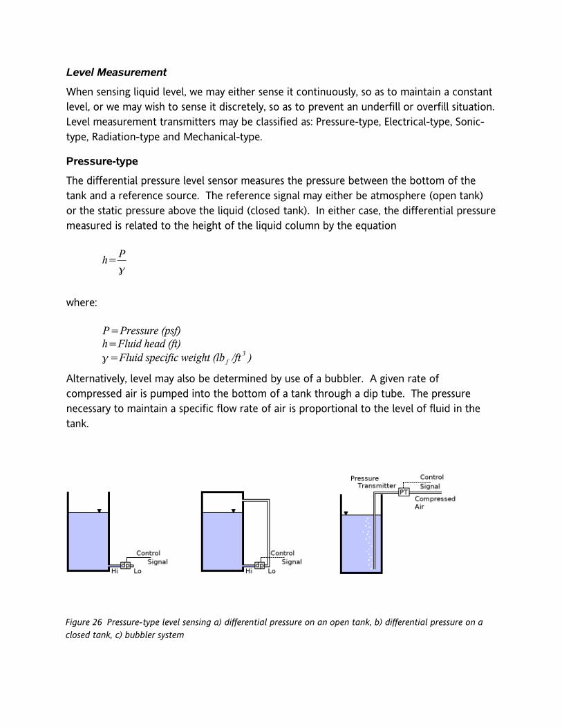
The differential pressure level sensor measures the pressure between the bottom of the tank and a reference source. The reference signal may either be atmosphere (open tank) or the static pressure above the liquid (closed tank). In either case, the differential pressure measured is related to the height of the liquid column by the equation

h=P

where:

P=Pressure (psf)h=Fluid head (ft)=Fluid specific weight (lb f /ft 3 )

Alternatively, level may also be determined by use of a bubbler. A given rate of compressed air is pumped into the bottom of a tank through a dip tube. The pressure necessary to maintain a specific flow rate of air is proportional to the level of fluid in the tank.

Figure 26 Pressure-type level sensing a) differential pressure on an open tank, b) differential pressure on a closed tank, c) bubbler system

Electrical-type

Electrical level sensors work on the principle of detecting changes in capacitance, resistance, or conductance when the sensor probe is submerged in the liquid. First, consider an electrical capacitor. A capacitor consists of two conductive plates electrically isolated from one another by a dielectric material. If the two plates are at different voltage potentials, a charge is stored. This storage capability is referred to as capacitance. A capacitance level detector is constructed of two conductors submerged in the liquid. The liquid acts as a dielectric. When the liquid level changes, the dielectric constant changes, thus the capacitance of the probe changes. This capacitance is measured and related to liquid level.

Resistance probes work in a very similar manner; in fact, resistance probes and capacitance probes often look identical. This probe measures the electrical resistance of the liquid separating the probes. As the liquid level changes, so does the measured resistance.

Conductance level transmitters tend to be used to measure discrete levels of fluid; often a high or low level. As the liquid covers or uncovers the probe, the conductance of the probe changes. If used as a high/low level, the signal is sent to an alarm for appropriate action.

Another class of level transmitters emits electromagnetic or sound energy and detects the passage of that energy through the liquid medium. The primary types of transmitters are ultrasonic, nuclear, microwave, and radar. Ultrasonic detectors emit sound waves and time the reflection of the sound wave from the liquid surface. Radar works in essentially the same way except the wave emitted is an electromagnetic wave in the high-frequency radio range rather than a sound wave. The difference is important when one realizes the speed of sound is dependent upon the medium through which a sound wave travels. Thus temperature and humidity affect the performance of ultrasonic transmitters. On the other

Figure 27: Capacitance and Resistive Level Sensors

hand, the propagation of electromagnetic waves is independent of temperature and humidity. Microwave detectors work similarly to radar detectors. An emitter sends a microwave signal in the direction of the liquid surface. A receiver detects the reflected signal, which is related to liquid level. The use of microwave detectors must be analyzed carefully since different materials attenuate microwaves differently.

Nuclear transmitters emit low-level gamma waves. Nuclear transmitters have the advantage of being able to detect liquid level through the walls of a tank. The propagation of a gamma wave is dependent upon the material through which the gamma wave travels. If several emitters are placed vertically along the wall of a tank with receivers placed opposite the emitters, the fluid level of the tank is easily determined.

Sensor Sensitivity

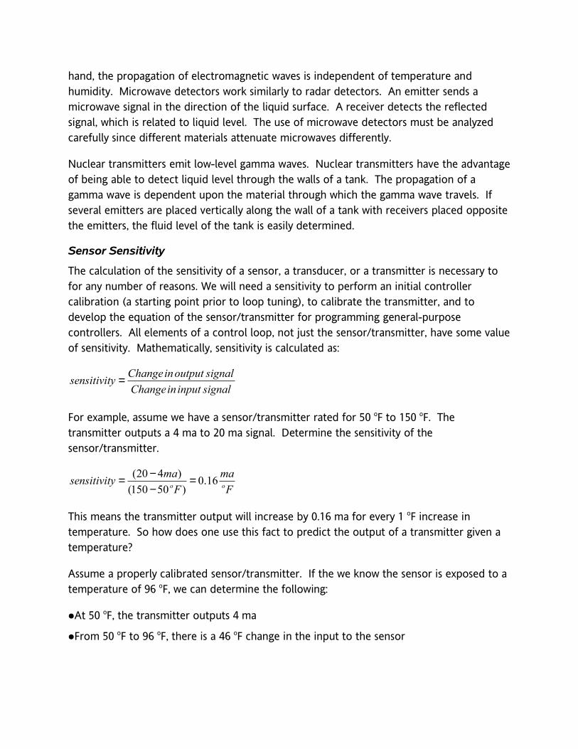
The calculation of the sensitivity of a sensor, a transducer, or a transmitter is necessary to for any number of reasons. We will need a sensitivity to perform an initial controller calibration (a starting point prior to loop tuning), to calibrate the transmitter, and to develop the equation of the sensor/transmitter for programming general-purpose controllers. All elements of a control loop, not just the sensor/transmitter, have some value of sensitivity. Mathematically, sensitivity is calculated as:

Changeinoutput signalsensitivity

Changein input signal=

For example, assume we have a sensor/transmitter rated for 50 oF to 150 oF. The transmitter outputs a 4 ma to 20 ma signal. Determine the sensitivity of the sensor/transmitter.

(20 4 )0.16

(150 50 )o o

ma masensitivity

F F

−= =−

This means the transmitter output will increase by 0.16 ma for every 1 oF increase in temperature. So how does one use this fact to predict the output of a transmitter given a temperature?

Assume a properly calibrated sensor/transmitter. If the we know the sensor is exposed to a temperature of 96 oF, we can determine the following:

●At 50 oF, the transmitter outputs 4 ma

●From 50 oF to 96 oF, there is a 46 oF change in the input to the sensor

●46 0.16 7.36o oF x ma F ma= This represents the change in output signal from the transmitter

●Since the output at 50 oF is 4 ma, then at 96 oF, we will have 4 + 7.36 = 11.36 ma total output signal.

The process above is independent of the signals measured. As another example, assume a pneumatic static pressure transmitter with an application range of -0.25 in w.g. to 1.75 in w.g. The sensitivity of this transmitter is:

( )(15 3 )

6(1.75 0.25 . . .) . . .

psi psisensitivity

in w g in w g

−= =− −

If we wish to predict the output at a pressure reading of 0.45 in w.g., we would do the following:

●At -0.25 in w.g., the transmitter outputs 3 psi

●From -0.25 in w.g. To 0.45 in w.g. is a 0.70 in w.g. change in the input to the sensor

●0.70 . . . 6 4.2. . .

psiin w g psi

in w g× = This represents the change in output signal

●Since the output at -0.25 in w.g. Is 3 psi, then at 0.45 in w.g., we will have 4.2 + 3 = 7.2 psi total output signal.

The equation of a sensor

Sometimes, it is appropriate to write the defining equation for a sensor. This is useful when calibrating sensor/transmitters and is essential when programming general purpose digital controllers. Fortunately, sensor/transmitters are linear and can be defined with the equation for a straight line, y mx b= + . When applied, it can be written in a more descriptive form as:

output sensitivity input offset= × +

For example, lets assume a flow sensor/transmitter capable of sensing a flow rate from 0 to 100 gpm. The sensor/transmitter outputs a signal of 2 to 10 volts over the sensing range. Write the equation for this unit.

●We can define sensitivity as: ( )

( )10 2

0.08100 0

v volts

gpm gpm

−=

−

●Now we need to find offset. We can do this by writing the equation around a known point. In this case, we know the transmitter outputs 2 volts when flow rate is 0 gpm. We

also know the output is 10 volts when the flow rate is 100 gpm. We can use either of these points to calculate offset. Both calculations are shown below.

2 0.08 0

( 2 )

voltsvolts gpm offset

gpm

offset volts

= × +

=

10 0.08 0

( 2 )

voltsvolts gpm offset

gpm

offset volts

= × +

=

●Regardless of which point you choose to determine the value of the offset, the final

equation is: 0.08 2volts

output input voltsgpm

= × +

Now it's a simple matter of substituting a given gpm flow rate for the input variable to calculate the expected output signal. For example, to determine the output of the transmitter at a flow rate of 56 gpm, we can write:

0.08 56 2 6.48volts

output gpm volts voltsgpm

= × + =

Notice this is identical to what we did above. It is just a more formal way of handling the same thing.

Accuracy and precision

When selecting a sensor-transmitter, one concern is how well the actual output of the transmitter conforms to the intended output. Such a specification consists of a measure of

accuracy, precision, deadband, hysteresis, and reproducibility. In layman's terms, accuracy and precision are often used interchangeably. In actuality, they have entirely different meanings. Accuracy is defined as the error between the measured value and the true value

a) Conformity b) Repeatability

Figure 28: Conformity and repeatability of an analog signal

of the process variable. It is also referred to as conformity or linearity. Figure 28(a) is a graphic depiction of accuracy.

Precision refers to how repeatable a measurement is. As such, it is often referred to as repeatability. A measurement may be precise, but not accurate. The Figure 29 illustrates the difference. Assume a hunter is target shooting. The goal is to hit the target in the center. Target 'a' illustrates the hunters aim is more or less 'on target'. But the shots are not closely grouped, indicating the hunter's aim may be accurate but not precise (repeatable). On the other hand, target 'b' in the graphic illustrates the hunter's aim is off center. However, all shots are closely grouped, thus the hunter's aim is precise (repeatable), but not accurate. Target's 'd' and 'e' show the same results, but with a stray shot. This would be considered random error and is often ignored when defining an accuracy specification.

Although we desire both a high degree of precision and accuracy for sensors installed in a control loop, precision is more important than accuracy. If the measurement capability of the sensor/transmitter is very repeatable, the control system will respond in a predictable manner, even if it is not accurate. Any loss of accuracy may be compensated artificially by adjusting the manual reset or the set point of the controller.

Deadband refers to a range of change in process variable over which there is no change in output. A mechanical equivalent is the backlash between a driven gear and the driver gear. When the driver is at a constant speed in one direction, the driven gear also rotates at a constant speed. If one was to slowly stop the rotation of the driver, then reverse direction,

a) Accuracy, no precision b) Precision, no accuracy c) Accuracy and Precision

d) Accuracy with e) Precision f) No accuracy random error with random error No precision

Figure 29: A graphic representation of precision and accuracy

the driver will rotate a small amount before the teeth of the driver contact the teeth of the driven gear. This is referred to as backlash and is analogous to deadband in a sensor. When the value of the controlled variable stops increasing, then begins to decrease, the output of the sensor will remain at a constant level for some small change in the process variable.

Hysteresis is a phenomenon in which the response of a physical system to an external influence depends on both the present magnitude of that influence and on the previous history of the system. A familiar example is a thermostat controlling a furnace with a set point temperature of T0. When the room temperature drops below T0 to some temperature T1, the furnace is turned on. As the room temperature rises through the set point to some higher temperature T2, the furnace turned off. As such, for temperatures less than T1, the furnace is always on and for temperatures above T2, the furnace is always off. Between the temperatures of T1 and T2, the furnace may be on or off. Whether it’s on or off is dependent on which of the two temperatures, T1 or T2, occurred most recently. Hysteresis and deadband are illustrated graphically in Figure 30. When accuracy, precision, deadband and hysteresis are combined, the response of a sensor might look like Figure 31.

a) Deadband b) Hysteresis c) Deadband + Hysteresis

Figure 30: The effects of deadband and hysteresis on a desired transmitter signal. The dotted line represents the desired transmitter signal. a) the affect of deadband without hysteresis, b) the affect of hysteresis without deadband, c) the affect of deadband and hysteresis. Graph 'c' is the typical scenario.

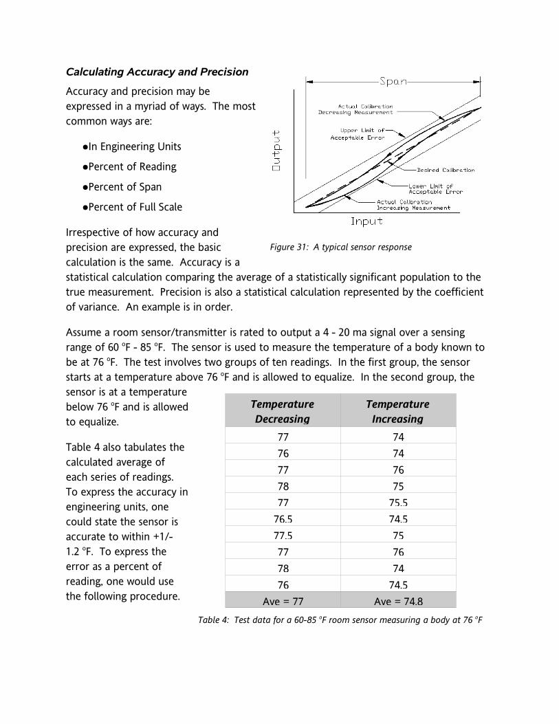
Calculating Accuracy and Precision

Accuracy and precision may be expressed in a myriad of ways. The most common ways are:

●In Engineering Units

●Percent of Reading

●Percent of Span

●Percent of Full Scale

Irrespective of how accuracy and precision are expressed, the basic calculation is the same. Accuracy is a statistical calculation comparing the average of a statistically significant population to the true measurement. Precision is also a statistical calculation represented by the coefficient of variance. An example is in order.

Assume a room sensor/transmitter is rated to output a 4 - 20 ma signal over a sensing range of 60 oF - 85 oF. The sensor is used to measure the temperature of a body known to be at 76 oF. The test involves two groups of ten readings. In the first group, the sensor starts at a temperature above 76 oF and is allowed to equalize. In the second group, the sensor is at a temperature below 76 oF and is allowed to equalize.

Table 4 also tabulates the calculated average of each series of readings. To express the accuracy in engineering units, one could state the sensor is accurate to within +1/-1.2 oF. To express the error as a percent of reading, one would use the following procedure.

Figure 31: A typical sensor response

Temperature Decreasing

Temperature Increasing

77 7476 7477 7678 7577 75.5

76.5 74.577.5 7577 7678 7476 74.5

Ave = 77 Ave = 74.8Table 4: Test data for a 60-85 oF room sensor measuring a body at 76 oF

The calculated error for this sensor as temperature is decreasing is:

% 100

77 76% 100 1.3%

76

x xError

x

Error

−= ×

−= × =

The calculated error for this sensor as temperature is increasing is:

74.8 76% 100 1.6%

76Error

−= × = −

The accuracy for this sensor could be stated as +1.3/-1.6 % of reading.

To express the percent error in terms of sensor span, one would use the same procedure as above except the divisor would be the span of the sensor. The range is 60 oF - 85 oF and the span is 25 oF. Thus the accuracy would be +4/-4.8 % of span.

Finally, accuracy can be expressed in terms of full-scale reading. Since full-scale reading is 85 oF, the accuracy specification would be +1.1/-1.4 % of full-scale reading.

The calculation of precision involves the calculation of the coefficient of variance. This calculation is performed as follows:

( ) 2

1:

StdDevCoeff of Var

x

StdDev Variance

x xVariance

nwhere n sample size

=

=

−=

−=

∑

Temperature Decreasing

Reading (x) x x− ( ) 2x x−

77 0 076 -1 177 0 078 1 177 0 0

76.5 0.5 0.2577.5 -0.5 0.2577 0 078 1 176 -1 1

77x = ( ) 24.5x x− =∑

Table 5: Calculation of precision for 60-85 oF sensor on decreasing temperature

Referring to Table 5, we can finish the calculation of precision as follows:

4.50.5

10 1

0.5 0.707

0.707100 0.9%

77

Variance

StdDev

Coeff of Var x

= =−

= =

= =

In a similar fashion, the precision for this sensor on increasing temperature can be shown to equal 1.0 %. Thus the precision of this sensor is +0.9/-1.0 %.

Temperature Increasing

Reading (x) x x− ( ) 2x x−

74 -0.8 0.6474 -0.8 0.6476 1.2 1.4475 0.2 0.04

75.5 0.7 0.4974.5 -0.3 0.0975 0.2 0.0476 1.2 1.4474 -0.8 0.64

74.5 -0.3 0.0974.8x = ( ) 2

5.55x x− =∑Table 6: Calculation of precision for 60-85 oF sensor on increasing temperature

Accuracy and precision for a system

It is often necessary to determine the overall accuracy and precision for a system composed of multiple components. We can do so by either determining the algebraic error or the probable error of the system. The algebraic error is determined by simply taking the algebraic sum of the errors. This has the advantage of simplicity. However, it is extremely conservative. It assumes each component provides a maximum error at the same time. Although theoretically possible, it is not a probable scenario.

Calculation of probable error is a bit more realistic as to the magnitude of error one may expect from a system. It is simply equal to the square root of the sum of the squares of the individual errors

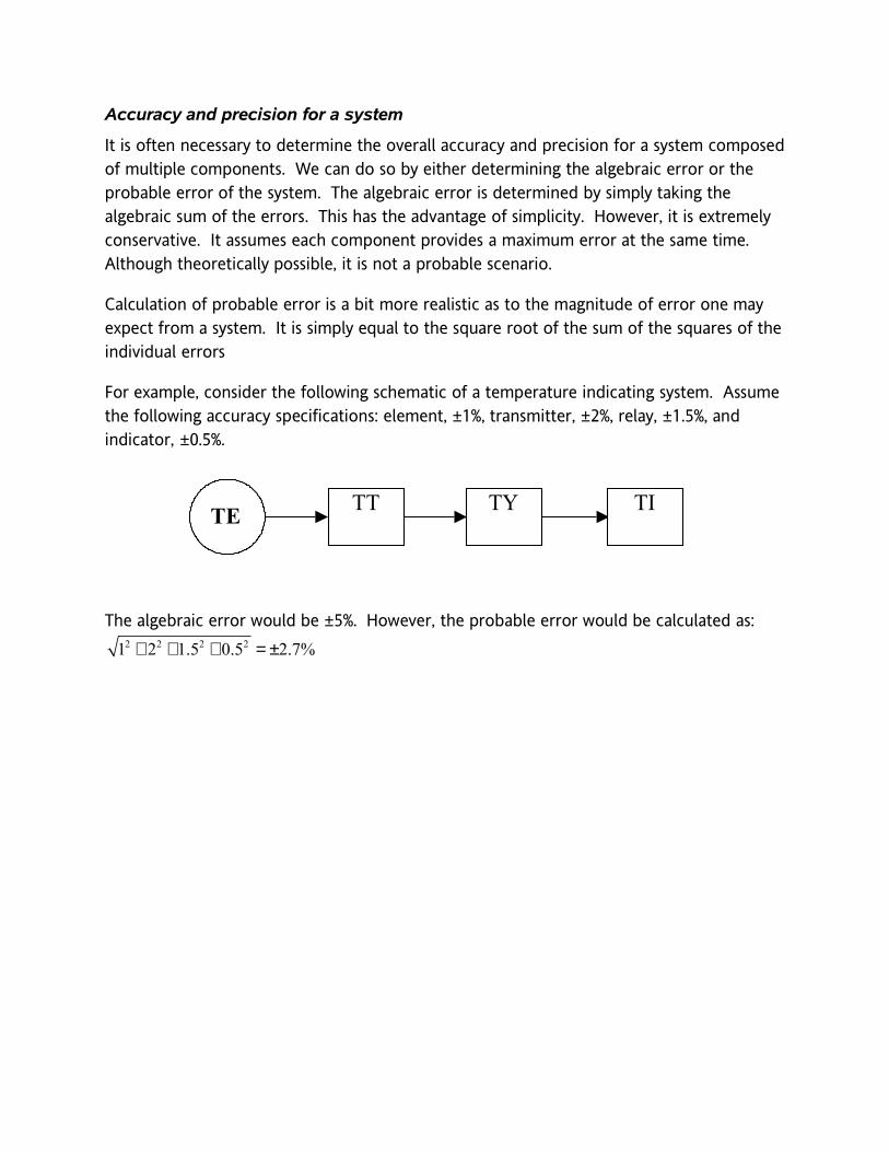
For example, consider the following schematic of a temperature indicating system. Assume the following accuracy specifications: element, ±1%, transmitter, ±2%, relay, ±1.5%, and indicator, ±0.5%.

The algebraic error would be ±5%. However, the probable error would be calculated as:2 2 2 21 2 1.5 0.5 2.7%+ + + = ±

TE TT TY TI