Embed Size (px)
Citation preview

CODE CODEN:LUTEDX/(TEIE-5357)/1-61/(2015)
Sensorless Control for Dynamic
Testing of PMSMs
Division of Industrial Electrical Engineering and Automation Faculty of
Engineering, Lund University

Sensorless Control for Dynamic Testing of
Permanent Magnet Synchronous Machines
Henrik Rydin Malmqvist
June 25, 2015
Abstract
This thesis investigates if it is possible to use the dynamic braking
test method together with sensorless control. A literature study is con-
ducted about di�erent sensorless methods in order to �nd methods that
�ts the application. From the litterature study are two sensorless meth-
ods implemented and simulated in Matlab Simulink. The results from the
simulations shows that when using the two methods together it is pos-
sible to test a PMSM in all possible current combinations. However for
some current combinations are the rotor position estimation not perfect
which leads to less accuracy for the results from the dynamic braking test
method.
2

.
3

Contents
1 Introduction 6
1.1 Structure of the thesis . . . . . . . . . . . . . . . . . . . . . . . . 61.2 Background . . . . . . . . . . . . . . . . . . . . . . . . . . . . . . 61.3 Project goals . . . . . . . . . . . . . . . . . . . . . . . . . . . . . 71.4 Method . . . . . . . . . . . . . . . . . . . . . . . . . . . . . . . . 71.5 Limitations of the master project . . . . . . . . . . . . . . . . . . 7
2 The PMSM 9
2.1 Transformations of a three phase system . . . . . . . . . . . . . . 92.2 Modeling of the PMSM . . . . . . . . . . . . . . . . . . . . . . . 102.3 Torque creation of the PMSM . . . . . . . . . . . . . . . . . . . . 132.4 The inverter for the PMSM . . . . . . . . . . . . . . . . . . . . . 14
3 Dynamic testing of PMSMs 16
3.1 Flux and Torque calculation using voltage and current . . . . . . 163.2 Torque calculation using moment of inertia and acceleration . . . 17
4 Methods for sensorless control 19
4.1 High frequency injection sensorless methods . . . . . . . . . . . . 194.1.1 Rotating voltage injection . . . . . . . . . . . . . . . . . . 204.1.2 Pulsating voltage injection . . . . . . . . . . . . . . . . . . 204.1.3 Pulse injection . . . . . . . . . . . . . . . . . . . . . . . . 21
4.2 Fundamental excitation signals sensorless methods . . . . . . . . 214.2.1 Open loop methods . . . . . . . . . . . . . . . . . . . . . 214.2.2 Closed loop methods . . . . . . . . . . . . . . . . . . . . . 224.2.3 Selection criterions . . . . . . . . . . . . . . . . . . . . . . 23
4.3 Voltage injection method . . . . . . . . . . . . . . . . . . . . . . 244.4 Open Loop . . . . . . . . . . . . . . . . . . . . . . . . . . . . . . 26
5 Simulation model 29
5.1 Model of PMSM . . . . . . . . . . . . . . . . . . . . . . . . . . . 295.2 Inverter . . . . . . . . . . . . . . . . . . . . . . . . . . . . . . . . 305.3 PI current controller . . . . . . . . . . . . . . . . . . . . . . . . . 315.4 Current provider . . . . . . . . . . . . . . . . . . . . . . . . . . . 315.5 Sensorless methods . . . . . . . . . . . . . . . . . . . . . . . . . . 325.6 Testing . . . . . . . . . . . . . . . . . . . . . . . . . . . . . . . . . 34
6 Results 36
6.1 Pulsating injection rotor position estimator . . . . . . . . . . . . 376.2 Open Loop rotor position estimator . . . . . . . . . . . . . . . . 41
6.2.1 Motor parameters obtained by a second iteration . . . . . 466.2.2 Compensation . . . . . . . . . . . . . . . . . . . . . . . . 49
7 Conclusions 53
7.1 Is sensorless control useful in the test method? . . . . . . . . . . 537.2 Future work . . . . . . . . . . . . . . . . . . . . . . . . . . . . . . 53
Nomenclature 60
4

.
5

1 Introduction
In this section are background information, scope, goals and method presented.
1.1 Structure of the thesis
This thesis starts with a short background and description of the problem, laterfollows the project goals for solving the problem. Then a short theoreticalintroduction is given to provide the reader some basic information. After that,a description over what has been conducted and results from the simulationsare presented. The last part of the report contains a conclusions section, futurework and a reference list.
1.2 Background
According to the UNFCCC, the climate change is the most important challengeto solve for the survival of mankind. UNFCCC also states that the human con-tribution to the climate change by burning fossil fuel is signi�cant, the trans-portation on land accounts for 13.1% of the total emission of green-house gasesfrom human activity [1]. To reduce the emission of green-house gases from ve-hicles, the European Union has made legislations that set standards to regulatethe green-house gas emission from new vehicles [2]. To meet up to those stan-dards, the automotive industry has started to look at bio-fueled, hybrid electric,electrical and hydrogen vehicles [3]. In the last three solutions it is required toequip the vehicle with electrical machines for propulsion and regeneration.
When the electrical machines are becoming more common in vehicle applica-tions, it is getting more and more important for the automotive industry to�nd easy ways of testing electrical machines. As an answer to that matter, theIndustrial Electrical engineering and Automation division at Lund Universityis working on a project that aims to investigate and develop a new method fortesting electrical machines [4]. The advantages with the new method are thatit is less time consuming and no torque sensor or breaking machine are neededduring the testing [4]. A typical test sequence with the new method is that themachine is accelerated to a pre-de�ned speed and when that speed is reached, itis braked and accelerated to the same speed in the opposite rotational direction[5].
Usually, to control a PMSM e�ciently the information about the rotor positionis needed [6]. The more conventional way to obtain the rotor position is to usea rotor position sensor. Because of some drawbacks with using rotor positionsensors such as calibration, it was decided that the ability of using sensorlesscontrol in the dynamic test bench should be investigated.
6

1.3 Project goals
The project goals were set up to make it possible to verify if this thesis is solvingthe problem that was formulated above.
• De�ne the requirements that the sensorless control strategy needs to ful�llin order to be used in dynamic testing.
• Conduct a literature study to identify which di�erent sensorless controlstrategies that exist and evaluate their advantages and drawbacks regard-ing the test application.
• Research and decide which sensorless control method or methods could besuitable to be used in the new testing method that is under developmentregarding the demands for the test method.
• Implement a simulation model with regards to evaluate if the sensorlesscontrol method gives satisfying results.
1.4 Method
This project starts with literature study of the new dynamic test method forPMSMs. A speci�cation list is created that contains the needs and demands ona new sensorless control method for the new dynamic test method application.
A literature study is conducted on di�erent sensorless control methods forPMSMs. In order to start the literature study two articles containing anoverview of di�erent techniques for sensorless control methods are read. Thenthe techniques that are estimated to �t to the application are investigated morecarefully.
The sensorless control methods that are expected to �t the dynamic test ap-plication are implemented in Matlab Simulink in order to see if they work. InMatlab Simulink the implemented sensorless methods are used in the dynamictest method application and the results are compared with results obtained withrotor position sensor.
1.5 Limitations of the master project
This project focuses on giving a suggestion on a sensorless control method thatcan be used for the new testing method. Only the methods that are chosenfrom the literature study are simulated, in other words this thesis does not aimto simulate and compare di�erent sensorless control methods. To evaluate ifthe sensorless method is useful in this application, only simulations in MatlabSimulink are conducted and the machines �uxes and torque production arecalculated by the new test method.
The limitations of the simulation model are depending on the simpli�ed PMSMmodel that is used in Matlab Simulink. Since the �ux maps that are used inthe model are obtained from a real PMSM, it can be concluded that the modelis acting as a real motor as long as the currents are with in the area of the
7

�ux maps. Some deviations for the PMSM can be assumed to depend on theresolution of the �ux maps. The whole model is simulated in continuous timebut some parts such as the PI-controllers and digital �lters works in discretetime.
8

2 The PMSM
In this section some fundamentals about the PMSM and the modeling of thePMSM are presented. The information in this section can be found in manydi�erent books for electrical engineers such as [6] and [7].
The PMSM is usually a three phase electrical machine with windings in thestator and permanent magnets in the rotor. Since the PMSM is a synchronousmachine the velocity of the rotor follows the frequency of the current it is fedwith divided by number of pole pairs in the machine.
2.1 Transformations of a three phase system
The PMSM is often modeled in the two phase rotating reference frame, but inreality most PMSMs are 3 phase electrical machines. In order to go from a 3phase system to a 2 phase system di�erent transformations have to be done andthey are explained below.
A 3 phase system contains three vectors abc, that are shifted 120 degree betweeneach other, see �gure 1. One way to represent those three vectors is by takingthe resulting vector of the 3 phase system and divide it into two componentsaligned with the alpha and beta axis again, see �gure 1. The alpha beta systemcontains therefor two vectors that are changing amplitude in order to recreatethe resulting vector of the 3 phase system.
In some cases it can be unpractical to calculate with vectors that is varying itsamplitude so therefor a way of representing the 3 phase system with just twoaxes called d and q respectively is used. In �gure 1, to the left shows the dq axesversus the alpha beta axes. The dq vectors are instead of changing amplitude,rotating counterclockwise with the electrical angular frequency to recreate theresulting vector of the alpha beta system. The dq frame is due to its rotationalso referred to as the rotating reference frame.
9

α
jβ
ua
ub
uc
uα
uβ
2π3
α
jβ
uduq
uα
uβ
π2
Figure 1: abc representation versus α β and α β representation versus the dqrepresentation.
The matrix in equation 1 shows the transformation from 3-phase-system towards2 phase stationary reference frame α β representation. In equation 2 the inversetransformation is presented.
[uαuβ
]=
[ 23 − 1
3 − 13
0 1√3− 1√
3
]uaubuc
(1)
uaubuc
=
1 0
− 12
√32
− 12 −
√32
[uαuβ]
(2)
Equation 3 shows the transformation from α β representation to dq represen-tation.
[uduq
]=
[cos(θ) sin(θ)−sin(θ) cos(θ)
] [uαuβ
](3)
The inverse transform, from dq rotating reference frame to αβ representationis shown in equation 4. [
uαuβ
]=
[cos(θ) −sin(θ)sin(θ) cos(θ)
] [uduq
](4)
2.2 Modeling of the PMSM
The PMSM is usually modeled in the rotating reference frames, in Krishnansbook about PMSMs two equivalent circuits are presented, one dynamic and onein steady state including the iron losses [6].
10

Dynamic equivalent model
The equivalent dynamic circuit is shown in �gure 2, the resistor represents thevoltage drop over the windings which is due to the resistance in the wire thewinding is built from [6]. After the resistor follows the inductance which modelsthe induced voltage from variations in the �ux linkage [6]. Finally the inducedvoltage is depending on the �ux produced in the other axis which is showed in�gure 2 [6].
+
idRs Ld
+− ωLqiq
−
vd
+
iqRs Lq
+− ω(Ldid + Ψpm)
−
vq
Figure 2: Equivalent dynamic circuits for the d- and q-frame.
The voltage equation for the d-frame consists of three parts see equation 5.The �rst part shows the voltage drop over the windings represented by Rs.The second term shows the induced voltage from the winding in the same axis.Finally is the cross coupling term which consists of the induced voltage due tothe �ux produced from the windings and current in the q-axis [6].
vd = Rsid + Lddiddt− ωLqiq (5)
The equation for the q-voltage is shown in equation 6, notice that the q-voltageequation is similar to the d-voltage, only the voltage sign and the third term isdi�erent and that is due to the �ux created by the permanent magnets in therotor [6].
vq = Rsiq + Lqdiqdt
+ ω(Ldid + Ψpm) (6)
The linked �uxes are given by equation 7 and 8 [6]. The d-axis �ux consists oftwo terms where the �rst one is the �ux created by the current and winding inthe d-frame and the second term is the �ux that is created by the permanentmagnets. The �ux that is created in the q-axis is directly from the current andthe winding in the q-axle.
Ψd = Ldid + Ψpm (7)
Ψq = Lqiq (8)
11

Steady state equivalent model including iron losses
Since the dynamic test method only works when the motor is operating in steadystate mode, the equivalent circuit can be simpli�ed by removing the inductance[5]. In the equivalent circuit a resistance is also added in parallel to the voltagedrop and that is to represent the iron losses in the motor. Because of thedynamic test method structure with a voltage subtraction the iron losses willdisappear. This make calculations possible without knowing motor parametersmore about later in this thesis [5]. The steady state equivalent circuits areshown in �gure 3.
+
idRs
iod
+− ωLqiq
−
vd
icd
Rsf
+
iqRs
ioq
+− ω(Ldid + Ψpm)
−
vq
icq
Rsf
Figure 3: Equivalent steady state circuits with core losses for the d- and q-frame.
From the steady state equivalent circuits in �gure 3 have the voltage equationsthat is shown in equation 9 and 10 been derived [8].
vd = Rsid − ωLqioq (9)
vq = Rsiq + ωLdiod + ωΨpm (10)
The currents in the equivalent circuits are given by equation 11 and 12 belowthat can be obtained by simple current division [8].
iod = id − icd = id −ωLqioqRdf
(11)
ioq = iq − icq = iq −ωLdiod + ωΨpm
Rqf(12)
By combining equation 9, 10, 11 and 12 the equivalent circuit voltages can bewritten as shown in equation 15 and 16 [8].
vd = (Rs +ω2LdLqRsf
)id − ωΨq +ω2LqΨpm
Rsf(13)
vq = (Rs +ω2LdLqRsf
)isq + ωΨd (14)
12

In the equivalent steady state circuit the core losses are modeled as a resistor inparallel with the motor. The core losses are mainly hysteresis losses and eddycurrent losses [6].
Hysteresis losses occurs when a magnetic �eld has been a�ecting a ferromagneticmaterial. Then some of the dipoles are still aligned in the direction of themagnetic �eld even though it has been removed. The losses occur because itcosts more energy to align those dipoles that are still align with the old magnetic�eld in another direction[6].
Eddy current losses occurs when the iron is exposed to varying �uxes and thenan induced emf is created that generates a current in the opposite directionwhich costs energy [6]. The eddy current losses depends on the material in thecore and is proportional to the electrical frequency.
In [9] a third source of core losses is introduced as excess losses and it is alsolike the other two loss components depending on the material and the electricalfrequency. Below is the full equation for core losses presented according to [9]in equation 17.
Pfe = khωBβm + kc(ωBm)2 + ke(ωBm)1.5 (15)
Since the motor is a three phase motor the resistor is given in equation 16[5]. However because of the design of the dynamic test method the iron lossresistance will never be calculated in the test method.
Rf = 3(ωΨpm)2
Pfe(16)
2.3 Torque creation of the PMSM
The electrical machine is created to convert electrical energy to mechanicalenergy or vice versa. There are two ways for a salient pole PMSM to generatetorque [6].
The �rst torque producing component in the PMSM is presented here. A varyingmagnetic �eld created by the stator windings. Because of the materials inthe PMSMs rotor and their magnetic permeability the rotor is moved by themagnetic �eld to a position where the reluctance for the magnetic �eld lines issmaller. By varying the magnetic �eld that is created by the stator inductancesthe rotor will follow the �eld in order to reduce the reluctance and torque isproduced [6].
The second way for the PMSM to create torque is by using the windings inthe stator to create a rotating magnetic �elds then the permanent magnets inthe rotor will follow the magnetic �eld in the stator so that the magnetic anglebetween the stator and rotor will be kept near 0 degree.
From the torque equation it is possible to see the above mentioned ways ofcreating torque in the PMSM see equation 17. The �rst part only dependson the permanent magnets magnetization and the second part of the equation
13

depends on the reluctance di�erences between the two axes. In equation 17Te stands for the electromagnetic Torque, p stands for the number of magneticpoles in the machine, ψpm stands for the permanent magnets �ux, is stands forthe magnitude of the currents in both d and q axes in the stator, δ stands forthe torque angle, Ld and Lq stands for the inductance of the two axes.
Te =3
2
p
2
[ψpmissin(δ) +
1
2(Ld − Lq)i2ssin(2δ)
](Nm). (17)
Since the PMSM is a synchronous machine the rotor speed depends directlyon the frequency of the currents it is fed with and the number of pole pairs ofthe motor [6]. The rotor speed is shown in equation 2 where p stands for thenumber of pole pairs in the motor, the f stands for the electrical frequency.
ω =4πf
p(rad/s). (18)
2.4 The inverter for the PMSM
In order to run the PMSM at di�erent speeds a device that can feed the PMSMwith voltages at varying frequency is needed. In order to do so a two levelvoltage source PWM inverter is selected.
The inverter uses switches that turn on and o� DC voltages with a high fre-quency to create three phase voltages with variable frequency. The inverter thatis used in the Simulink model is a 3 phase 2 levels inverter. Which means thatfor every phase the inverter can give two voltage levels Vdc/2 and −Vdc/2. Tocreate the desired voltage the inverter uses the reference signal from the currentcontroller and a high frequent triangular wave. When the reference signal isabove the triangle wave then the switch is on and gives Vdc/2 and the switchgives −Vdc/2 when the reference signal is below the triangle wave, see �gure 4.
14

Figure 4: Shows how the inverter creates a voltage from a triangle waveand a reference wave. From: http://se.mathworks.com/help/physmod/sps/powersys/ref/pwmgenerator.html
The frequency of the triangular wave has to be at least 10 times the frequencyof the reference signal if the inverter should be able to create the correct outputsignal from the reference [7].
15

3 Dynamic testing of PMSMs
The procedure for the test method is presented in �gure 5, where the green lineis the q current, the blue line is the d current and the red line is the speed.
The method consists of a speed sequence that has to be performed. The speedsequence starts accelerate the machine to a negative pre-de�ned speed see thebottom left corner of the square in �gure 5. Then the machine is braked tozero speed and directly accelerated up to the pre-de�ned positive speed see theupper right corner of square in �gure 5.
When performing the test method the measurements of speed voltages andcurrents are needed, the measurements takes place when the test procedure iswithin the black square in �gure 5.
Figure 5: Test sequence when the new test method is performed, only themeasurements inside the rectangle are relevant for the test method.
The test method can be used to measure the linked stator �uxes. The dynamictest method consists of two methods to calculate torque, using voltages andspeed or by using the moment of inertia and acceleration.
3.1 Flux and Torque calculation using voltage and current
This method builds directly on the steady state equivalent model with corelosses and uses the voltage equations derived from that circuit.
From the voltage measurements during the test sequence when it is within thesquare in �gure 5, and are used according to the following equations on the nextpage. When calculating the linked stator �ux for the d-vector the voltage overthe q-axis is used and the measurement for when the machine is acceleratingis subtracted with the measurement for when the machine is braked for eachspeed. After the subtraction, the remaining parts of the voltage equation fromthe steady state equivalent circuit are the second term that contains the speedand the linked stator �ux. Since an addition has been performed and bothvoltages are at same speed the result is 2 times the speed times the linked
16

stator �ux in the d-axis. In order to get the linked stator �ux the equation isdivided by 2 times the speed see equation 19.
Ψd =vωq − v−ωq
2ω(19)
In order to get the stator �ux linkage in the q axis similar calculations areperformed as in equation 19 the only di�erence is that the voltage during brakingis being subtracted by the voltage during acceleration see equation 20. Thereason for the change in position of the voltages is due to the second term inthe voltage equation for the d voltage is negative see equation 9 and 10.
Ψq =v−ωd − vωd
2ω(20)
In order to be able to calculate the torque that is produced by the electricalmachine the currents are needed and they are assumed to be the mean value ofthe current for each speed when the machine is braking and accelerating.
Since the machine is held in steady state during the sequence in the square see�gure 5 the torque can be derived by multiplying the d linked stator �ux withthe q current minus the q linked stator �ux multiplied with the d current andmultiply it with the number of pole pairs see equation 21 [5].
Te =p
2(Ψdiq − Ψq id) (21)
3.2 Torque calculation using moment of inertia and accel-
eration
By using the same test sequence but instead measure the acceleration and cal-culate the moment of inertia on the rotor makes it also possible to calculate thetorque [5].
The rotor position is obtained by using the data from the rotor position sensor(θ) that is given by angular frequency. The acceleration of the electrical machineis how much the rotor is changing its speed for every time unit. In order to getthe acceleration the angular frequency from the rotor position is derived seeequation 22. Since the electrical machine is not ideal not all produced torquewill be used to accelerate or brake the machine and therefor another term Tlossthat represents the friction losses in the rotor has to be added in the equation.
dω
dt=ω(t)− ω(t− 1)
Tloss(22)
By multiplying the moment of inertia with the acceleration and braking foreach speed the mechanical torque can be obtained see equation 23 [5]. By
17

performing this calculation the Tloss will disappear since the friction will alwayspoint against the angular direction of the rotor.
T = Jdωω
dt +dω−ω
dt
2(23)
The dynamic test method has been proven to be accurate when used with arotor position sensor, according to [5] the di�erence in torque measurementsbetween the new test method and traditional test method are less than 0.5%.
For the new test method no additional brake machine is needed, only attachinga �ywheel on the rotor of the machine that is being tested may be needed.Because of that, the dynamic test method is much faster than a traditional testmethod for electrical machines [5]. In the article it is mentioned that the timefor performing test of an electrical machine with 100 measurement sequenceswill only need approximately 2 hours compared with the traditional test methodthat will use 5 to 6 hours for the same task.
18

4 Methods for sensorless control
To control a PMSM, three di�erent sensors are usually needed: two currentsensors and one rotor position sensor [6]. By using a sensorless control strat-egy the new test method can also be used for PMSMs that lacks rotor positionsensors[10]. According to di�erent research projects the sensorless control meth-ods can be divided in to two groups: fundamental excitation signals and Highfrequency injection [11] [12]. A tree graph is presented in �gure 6 that showshow the di�erent ideas of sensorless control are related to each other.
SensorlessControlmethods
Highfrequencysignal
injection
Pulseinjection
[11, 20-24]
Sinusoidalsignal
injection
Rotatingvoltageinjection[13-14]
Pulsatingvoltageinjection[15-19]
Fundamentalexcitationsignals
(back emf)
Open loopmethods[25-28]
Closed loopmethods
Reducedorder
observers[29-32]
Full orderobservers[33-35]
Figure 6: The relationship between di�erent methods for sensorless control.
4.1 High frequency injection sensorless methods
These methods requires an external high frequent signal injection besides cur-rent and voltage measurements. The external signal can be injected either inthe stationary reference frame (αβ-representation), or in the in the rotating ref-erence frame (dq-representation) [11]. The injected high frequent signal is usedto make the saliency of the electrical machine visible for the sensorless rotorposition estimation method [11]. Then di�erent methods are used in order toextract information about the error between the estimated rotor position andthe actual rotor position [12].
In order to make the estimated rotor position follow the real rotor positionan observer is needed [11]. The observer increases or decreases the estimatedrotor position and therefor minimizes the rotor position di�erence between theestimated rotor position and the real rotor position, the observer that is usedin one of the high frequency signal injection methods are explained in detail inthis chapter.
19

4.1.1 Rotating voltage injection
Rotating signal injection sensorless methods usually inject a high frequent volt-age (sinus and cosine voltages) in both α and β vector. In order to track therotor position the voltages that are measured are undertaken a heterodyningprocess. Then the signals are low-pass �ltered in order to get rid of the injectedsignal whereupon the d axis voltage is high pass �ltered to get rid of a positivedc current that is not useful for extracting the rotor position. By subtractingthe q voltage with the d voltage the di�erence between the actual rotor positionand the estimated rotor position is obtained. Then by adding a PID controllerthat act as a follower which aims to minimize the di�erence it is possible tofollow the real rotor position [13].
This sensorless control method is presented in the article as completely inde-pendent of rotor parameters instead, information about the torque is needed tokeep track of the rotor position [13]. It is also claimed that the injected voltagehas negligible e�ect on the performance of the method [13].
The two main components that a�ect the dynamic performance in this type ofsensorless control methods are: the phase delay of the �lter, and the responsesof the PID controller that is used as a follower.
In [14] a way of improving the dynamic performance of the rotating signal in-jection sensorless method is presented. The injected signal amplitude increaseswith increased speed and also a new follower to track the rotor positon is pre-sented. Since the follower uses a minimum of �lters in order to improve dynamicperformance it instead needs motor parameters. It is claimed that the sensorlesscontrol technique is able to handle 250% of the rated torque at standstill.
4.1.2 Pulsating voltage injection
The pulsating voltage injection sensorless methods are quite similar to the ro-tating voltage injection methods. The main di�erence is that the high frequencyvoltage is injected in the rotating reference frame instead of the stationary ref-erence frame.
A completely machine parameter insensitive sensorless control method is pre-sented in [15]. A saturation e�ect compensation method is presented by takingthe use of the rotor design of the machine. The main drawback with this methodis that the observer needs to know the torque that is produced by the machinein order to track the rotor position. In [16] the scheme is proven to work withboth IPMSM and machines with low saliency SMPMSM.
By injecting both positive and negative sequence pulsating signal it was possi-ble to detect the rotor position more accurate for machines with low salienceswithout including an observer dependent on machine parameters [17]. By syn-chronising the injected signal with the PWM inverter it is possible to get rid oflag e�ects and thereby obtain more accurate rotor position estimation [18].
Overall are both voltage injection methods quite similar in both theory and im-plementation, however for PMSM it has been found that pulse voltage injectionmethods are more common in literature [11]. A comparison study was performed
20

in [19] between two signal injection sensorless methods. It was concluded that ithas a small in�uence on the performance of the sensorless estimation dependingon if rotating voltages or pulsating voltages were injected. The only di�erencethat could be observed in this paper is that the error using pulsating voltageinjection is slightly smaller than the error using rotating voltage injection.
4.1.3 Pulse injection
In order to obtain the rotor position with this type of method are test volt-ages injected during short time intervals and the currents from the PMSM areanalyzed in order to obtained the rotor position [11]. Notice that this type ofsensorless method only works with salient pole PMSMs. Exactly when thosetest voltages are injected, the voltages and currents over the electrical machineare measured [20]. From the derivative of the currents the phase inductancesare identi�ed and since the inductance change depending on the rotor positionit is possible to track the rotor position [11].
A popular pulse injection technique is called INdirect Flux detection by On-lineReactance Measurements (INFORM), and follows a special pattern where theinverter is paused and special test voltage vectors are injected. The injectionsof the test vectors causes some current and torque ripple since the inverter thatis feeding the motor have to be paused in order to inject test voltages [21].This pulse injection method is not using any test voltages to estimate the rotorposition but since an alternative PWM has to be used the overall e�cency isdeclined by 15% which may a�ect the test method [22].
In order to reduce the main disadvantage with pulse injection methods a newpulse injection scheme is introduced in [23]. Normally pulse injections methodsare suitable for zero and low speed operation but in order to increase the speedlimit a new detection technique is used in [24]. One negative aspect by thismethod is that in order to calculate the �uxes the value of the q-inductance isneeded which means that the method requires a motor parameter.
4.2 Fundamental excitation signals sensorless methods
The methods in this section do not require any signal injections or similar.Instead they obtain the rotor position by voltage and or current measurementsfrom the motor. A drawback these kind of sensorless methods have is that theyperform relatively bad when used from stand still and in low speeds.
The sensorless control methods that use fundamental excitation signal can bedivided in to two groups of methods, open loop methods and closed loop methods[11].
4.2.1 Open loop methods
The open loop methods do not have any internal correction scheme which makesthem work poorly in low speed operations [11]. To be able to make the open loopmethods useful they have to be combined with a method for accelerating the
21

motor at zero and low speeds. That could be by energizing the stator accordingto a special pattern, by injecting a pulse pattern to the PWM inverter or byusing a signal injection sensorless method [6].
In [25] a open loop sensorless control method is presented that can be used inzero and low speed operation. This method does not us back EMF to track therotor position therefor it is possible to use for low and zero speed operation,instead this method uses the PWM pattern and voltage measurements over allphases in order to determine the rotor position. In order to obtain the rotorposition the inductances of the motor have to be known.
The paper �Indirect sensing for rotor �ux position of permanent magnet ac mo-tors operating over a wide speed range� [26]presents two ways of measurementsin order to obtain the third harmonic voltages, one that was direct measure-ment on the machines neural network or by measuring on the di�erent phases.The advantage with using the third harmonic voltages for obtaining the rotorposition is that it requires a minimum of �ltering especially when measuring onthe neural network.
By just measuring the voltages and currents from the electrical machine andthen performing an integration it is possible to get the back emf �ux vector fromwhich the rotor position can be obtained [27]. A rather complicated correctionalalgorithm is presented in order to prevent errors from the integrations that isperformed. Thus this sensorless method has a strong speed limitation whichmeans that this method is not useful for speeds under 1Hz angular velocity.
Another open loop method is based on the electrical steady state circuit in orderto obtain the back emf and therefrom obtain the di�erence between the rotorposition and the estimated rotor position [28]. This method does not use any�lters hence it will respond very fast to transients. As long as the currents arekept constant it is showed that this method performs accurately.
4.2.2 Closed loop methods
The closed loop methods usually contains some kind of model of the electricalmachine that is controlled to be able to correct the rotor position estimation,which makes the closed loop methods less sensitive to motor parameter varia-tions compare to open loop methods. This especially a�ect the sensorless controlin low speed operations [12]. The closed loop methods are divided in to two sub-groups depending on the complexity of the correction mechanism: reduced orderobserver and full order observers [11].
The full order observer usually contains both mechanical and magnetic modelof the electrical machine that is being controlled, this means that a lot of motorparameters for the actual motor that is being controlled is needed [11].
The reduced order observer is similar to the full order observer but usually doesnot contain the mechanical model of the motor, this means that you don't needto know the motor you are controlling as much like in the full order observercase [11].
22

Reduced order observers
In [29] two di�erent kind of motor model were used: a current model and avoltage model. In order to obtain the rotor position the real voltage or currentdepending on which motor model that is used are compared with the voltageor current from the model depending on the sign on the di�erence the rotorposition estimation will be increased or decreased.
A more machine parameter insensitive approach for sensorless control is pre-sented in [30]. An Extended Kalman Filter is used as the motor model and theback EMF in order to obtain the rotor position is derived from current mea-surements. The method was proven to work in both transient state and withdetuned motor parameters from standstill to high speed for IPMSMs.
In order to reduce the lag in the rotor position estimation the expected torqueis used as a feed forward input in [31], a similar approach is with few variationspresented in [32].
Full order observers
The �rst presented closed loop sensorless control strategy with full order ob-servers is presented in[33]. In this approach, all motor parameters are assumedto be constant. This can cause problem for the rotor position estimation whenthe motor is saturated. In order to reduce the problem with saturation andchanging motor parameter while the motor is running a sensorless control tech-nique is proposed in [34] using a Extended Kalman Filter as the reference model.
The method in [34] is claimed to perform well from high speeds down to 10%of the nominal speed of the motor. In order to make this type of sensorlesscontrol usable down to zero speed it needs to be used together with a signalinjection method. In [35], is a hybrid sensorless control method presented. In[36]it presents why low speed operation for closed loop methods is performingrelatively bad how to overcome those issues with low speed operation, are in-vestigated. It is concluded that when the speed decreases, the back-EMF whichincludes the rotor position information also decreases, which leads to the signalthat contains the rotor position information is drowned in noise created mainlyby the inverter and partly by the back-EMF harmonics. In order to make lowspeed operation possible the bandwidth in the observer is decreased and thatleads to side-e�ects as low robustness in the sensorless control method.
4.2.3 Selection criterions
According to knowledge retrieved from the literature study table 1 is developed,which from certain criterions grades the di�erent sensorless methods. It is im-portant to know that this is a brie�y grading for di�erent methods that is validfor the general case and some exceptions may exist but it is decided to insertthis �gure since it is very good way to inform the reader mainly advantages anddrawbacks that each method present.
23
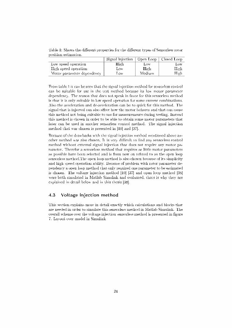
Table 1: Shows the di�erent properties for the di�erent types of Sensorless rotorposition estimation.
Signal injection Open Loop Closed LoopLow speed operation High Low LowHigh speed operation Low High HighMotor parameter dependency Low Medium High
From table 1 it can be seen that the signal injection method for sensorless controlcan be suitable for use in the test method because its low motor parameterdependency. The reason that does not speak in favor for this sensorless methodis that it is only suitable in low speed operation for some current combinations.Also the acceleration and de-acceleration can be to quick for this method. Thesignal that is injected can also a�ect how the motor behaves and that can causethis method not being suitable to use for measurements during testing. Insteadthis method is chosen in order to be able to obtain some motor parameters thatlater can be used in another sensorless control method. The signal injectionmethod that was chosen is presented in [10] and [37].
Because of the drawbacks with the signal injection method mentioned above an-other method was also chosen. It is very di�cult to �nd any sensorless controlmethod without external signal injection that does not require any motor pa-rameter. Therefor a sensorless method that requires as little motor parametersas possible have been selected and is from now on refered to as the open loopsensorless method.The open loop method is also chosen because of its simplicityand high speed operation ability. Because of problem with rotor parameter de-pendency a open loop method that only required one parameter to be estimatedis chosen. The voltage injection method [10] [37] and open loop method [38]were both simulated in Matlab Simulink and evaluated, thats is why they areexplained in detail below and in this thesis [38].
4.3 Voltage injection method
This section explains more in detail exactly which calculations and blocks thatare needed in order to simulate this sensorless method in Matlab Simulink. Theoverall scheme over the voltage injection sensorless method is presented in �gure7. Layout over model in Simulink
24

Current Controller + Inverter PMSM
Rotor Position Estimator
Feedback
iref uref uabc
iabc
θes
uhf
uhf
Figure 7: Shows the overall scheme for the signal injection rotor position esti-mator.
The injected voltage is decided by equation 24 where vc, is the voltage ampli-tude of the injected voltage and α is the frequency of the injected voltage. Itis important that the frequency of the injected signal is not the same as thefrequency from the rotor or the inverter, a typical frequency for the injected sig-nal is between 500 Hz and 2000 Hz [10]. The voltage amplitude should also beselected so a good signal to noise ratio will be achieved [11]. The high frequentvoltage can be injected in either α-axis or in β- axis. The voltage is injectedafter the PI-regulator in the current-control circuit [37].[
vαhvβh
]= vc
[cos(α)
0
], where α = ωct + φ (24)
The current response from the electrical machine and the injected voltage areshowed in equation 25 and after some calculations it leads to equation 26.
d
dt
[iαhiβh
]=
[1Lp
+ 1Ln
cos(2θr + θm) 1Ln
sin((2θr + θm)1Ln
= sin(2θr + θm) 1Lp− 1
Lncos(2θr + θm)
]
· Vc[cos(α)
0
](25)
[iαhiβh
]=
[Ip + In cos(2θr + θm)In sin(2θr + θm)
]· Vc
[cos(α)
0
], In =
VcωcLp
, Ip =VcωcLn
(26)
The currents in equation 26 are processed with a method called heterodyningwhich means that the signal is multiplied with 2sin(α). After that the signal isLow pass �ltered and the result can be seen in equation 27. The injected highsignal from equation 24 is now gone and now the signal contains a DC part, acosine signal that contains the rotor position information in the α frame and asinus with rotor information in the β frame.
25

[|iαh||iβh|
]= LPF
([iαhiβh
]· 2 sin(α)
)=
[Ip + In cos(2θr + θm)In sin(2θr + θm)
](27)
After this, the α part is multiplied with cos(θr) and the β part is multipliedwith sin(θr). Then θr comes from the feedback in the phase locked loop, seeequation 28. [
|iαh||iβh|
]·[
sin(2θe)cos(2θe)
](28)
In equation 29 the current from the �rst and second row in equation 28 issubtracted to eachother, and that leads to a single sinus function as can be thatcontains the rotor position error . It is towards this error the phase locked loopis working.
|iαh| sin(2θe)− |iβh| cos(2θe) = sin(2(θr − θe)) ≈ In2(θr − θe) (29)
The approximation in equation 29 is only valid for small errors, so the assump-tion only works when the phase locked loop is accurately tuned. The goal of thephase locked loop is to increase the rotor position θe so that θr-θe is as close tozero as possible, which means that the rotor position estimation is closely fol-lowing the real rotor position. The overall scheme of the signal injection basedrotor position estimator that is simulated in Matlab Simulink is shown below in�gure 8.
x
x
LPF
LPF
x
x
+ PI 1s
sin(2θe)
cos(2θe)
iα
iβ
2sin(α)
2sin(α)
−
θe
Figure 8: Shows the overall scheme for the signal injection rotor position esti-mator.
4.4 Open Loop
The overall layout of the set up with motor, inverter, controller and Open Looprotor position estimator is shown in �gure 9.
26

Current Controller Inverter PMSM
Rotor Position Estimator
Feedback
iref Uref Uabc
Uabc, iabc
θe
Figure 9: Shows the overall scheme for the Open Loop rotor position estimator.
The rotor position estimator block from �gure 9 is in more detail described by�gure 10 below.
abc -> αβ
Flux estimator
Current estimator
Calculation of ∆iq
Low Pass Filter PI-controller 1s
θ
Uabc, iabc
Uαβ , iαβ
ψαβ
iαβ
∆αβ
ω
Figure 10: Shows the calculation blocks for the Open Loop rotor position esti-mator.
Below every calculation from �gure 10 needed for this sensorless rotor positionestimator are presented. The source for this method is [38]. First the �ux is
27

estimated by integrating the voltage subtracted with the current and resistanceaccording to equation 30.
ψαβ =
∫(Vαβ −Rsαβ)dt (30)
Then the currents are estimated by following calculations in equation 31, whereθ is the estimated rotor position that is estimated by the method.
iα =1
L[ψα − ψmcos(θ] iβ =
1
L[ψβ − ψmcos(θ] (31)
The di�erence between the estimated and measured currents are calculated inequation 32.
∆iαβ = iαβ − iαβ (32)
Then the currents from equation 32 is transformed from αβ to dq-frames ac-cording to equation 33.
∆iq = −∆iαsin(θ) + ∆iβcos(θ) (33)
∆iq is the signal that goes to the PI controller that works to minimize the errorby increasing ∆iq, therefor it can be said that the PI-controller is tracking thespeed. The signal from the PI-controller is then integrated to get the rotorposition.
28

5 Simulation model
This section has been created to inform the reader in detail about how the modelfor validating the sensorless control strategy with the test method is created.Figure 11 shows the simulation model. It contains the following blocks: referencecurrents, signal injection, current controler, PMSM model, simulation data androtor position estimator.
Figure 11: Shows a overview scheme of the simulation model that was used.
5.1 Model of PMSM
In the beginning of the project the methods are simulated together with alinear model of an PMSM. In reality the PMSM does not act linnear because ofsaturations e�ects. This means that the PMSM for example does not necessarilycreate twice as much torque when the current is doubled. To create a morerealistic model of the PMSM �ux maps that are obtained from a real electricalmachine in this PhD thesis [39] are used. Since the �ux maps are retrived frommeasurement with the new dynamic breaking test method of a real PMSM, itcan be assumed that the model of the PMSM acts like the real PMSM in termsof losses and saturation.
29

Figure 12: Shows the model of the PMSM that is used in the simulations. Themodel is originally made by Mats Alaküla and are just slightly modi�ed in orderto use the �ux maps.
As can be seen in �gure 12 the model of the PMSM that is used �rst transformsthe incoming voltages to the rotating reference frame (dq). Then by performingan integration of the incoming voltages minus the resistance times the currentsand minus the speed times the inverse �uxes the �uxes are calculated as canbe seen in equation 34. Then depending on the �ux values the currents wasobtained from the currents maps that are derived from the �ux maps.[
Ψd
Ψq
]=
∫ [vdvq
]−Rs
[idiq
]− ωel
[−Ψd
Ψq
]dt (34)
The torque from the PMSM model is calculated according to formula 35 belowwhere p is the number of poles for the machine.
Ψd · iq −Ψq · id = Tmech, Tel = Tmech ·p
2(35)
The rotor speed is calculated by integrating the torque minus the breaking powerfrom an external object Ti see equation 36, where J is the mass of the rotor.
ωmech =
∫(Tmech − Ti) ·
1
Jdt, ωel = ωmech ·
p
2(36)
5.2 Inverter
The inverter contained 3 switches that feed the PMSM-model with di�erentpositive and negative DC-currents. The switch contained a triangular wave
30

with the frequency of 10kHz. The inverter are feed by Vdc and -Vdc whichhas the following voltage levels 150V and -150V. The simulation model of theinverter that is used can be seen in �gure 13.
Figure 13: Shows the inverter that was used in the simulations.
5.3 PI current controller
The PI-controller that is used in the simulations is taken from one of the homeassignments in the power electronics course in IEA LTH. The high voltage in-jection is performed just after the current controller as can be seen in �gure14.
Figure 14: Shows the current controller block.
5.4 Current provider
The current reference provider that can be seen in �gure 15, is created to givethe correct reference currents to the current controller according to the test
31

method for PMSMs. The current provider also make it possible to use twodi�erent current combinations that switched depending on the rotor speed, thisfunction is useful when using the pulsating injection method to accelerate thePMSM and then let the open loop method take over. The relay signal had thevalue of 2 before and after the measurements for the test method is performed.
Figure 15: Shows the block for reference currents.
5.5 Sensorless methods
Since this master project contained two di�erent sensorless rotor position esti-mation methods both of them are implemented in Simulink. To change whichsensorless method that is used during simulations, a switch is set up as can beseen in �gure 16.
32

Figure 16: Shows the two sensorless methods block and a switch that changemetod depending on the rotor speed.
The block for decoding the current response from the PMSM followed the de-scription that has been given in earlier chapters are presented in �gure 17. Anissue with this method is to �nd a proper �lter to get rid of the high frequentsignal. Since the observer needed to get the rotor position with as small phaselag as possible a Bartlett Hanning �lter design with the cut frequence of 700Hzwas selected. The PI-controllers gain are selected from the article that presentedthe sensorless control strategy with the values of kp = 500 and ki = 1000 [37].
33

Figure 17: Shows the blocks that was used for decoding the signals from thePMSM in the signal injection method.
The open loop method is easy to build since the method is well described in[38] and the Simulink implementation is shown in �gure 18. The gains of thePI-controler are found by testing di�erent PI gain values and compare how wellthe sensorless method is following the rotor position. It is concluded that thekp should be 15 and ki should be 584.
Figure 18: Shows the blocks that was used for the open loop method.
5.6 Testing
To evaluate the di�erent sensorless methods that is presented in this project asimple script in Matlab is written so that all the results are created in a similarway. The script runs the simulation for di�erent currents injected to the PMSMin the dq frame and the result is then saved in a matrix where the the x and y
34

axis represents the d and q -currents. To illustrate the results the result matrixsis plotted by a 3d plot function called surface in Matlab.
In order to test the di�erent sensorless methods �ux maps are taken from anotherproject and used in this thesis [39]. In that thesis the dynamic braking methodis used with the following current combinations id = 0:-70 A and iq = 10:70A, that is also why those current combinations are used in order to test thesensorless methods.
The measurements for the open loop sensorless method the results is onlyrecorded when the motor has reached a speed of minimum 60 rad/s. The reasonfor this is because the sensorless method does not work at all for speeds under60 rad/s.
35

6 Results
This section presents the results from the di�erent rotor position estimationmethods used with the dynamic test method.
First are the �uxes that has been used for simulating the motor in MatlabSimulink presented. The �uxes have been created in [39] and have been obtainedby using the new dynamic test method together with a rotor position sensor.
In �gure 19 it can be seen that the d-�ux depends on the amount of the d-current the PMSM is feed with. Just as it is described in equation 7 earlier.In �gure 20 the q-�ux is presented it can be seen that it depends on how muchq-current the PMSM is feed with and that is correlating to how the q-�ux isdescribed in equation 8.
The results that is important to get is the d-�ux and q-�ux because from thatinformation the torque can be calculated. It is the same parameters that thenew test method needs to obtain.
Figure 19: Ψd under di�erent current combinations that have been found viathe dynamic testing method during sensored mode of the PMSM [39].
36

Figure 20: Ψq under di�erent current combinations that have been found viathe dynamic testing method during sensored mode of the PMSM [39].
6.1 Pulsating injection rotor position estimator
The main purpose for this method in this master project is to obtain the motorparameters that is needed for the open loop sensorless method. That is becauseof the pulsating injection can create saturations e�ects on the PMSM and thatmakes the values obtained by this method not reliable for the new test method.So the signal injection methods main purpose is to obtain the ψpm and ψd valuesfrom which the Ld and ψpm can be obtained. Those are the motor parametersused by the open loop method.
A full cycle for one current combination in this method showing speed, currents,rotor position error and torque is presented in �gure 21. In �gure 22 a cycle foranother current combination is presented, it can be seen that the rotor positiontracking in this cycle is not very successful.
37

Figure 21: Shows a test sequence with the pulsating injection method.
Figure 22: Shows a test sequence were the pulsating injection method is notperforming very well.
A problem that was found with the signal injection method is that it could onlytrack the rotor position for a few current combinations. In order to make thesignal injection method tracking the rotor position for more current combina-tions the rotor inertia was increased. It is shown in �gure 23 that increasingrotor inertia does not help this method to keep track of the rotor position whenincreasing the �eld weakening current id.
38
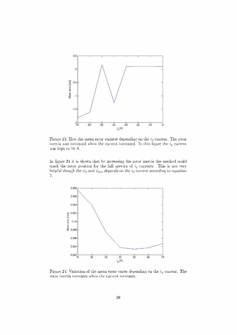
Figure 23: How the mean error variates depending on the id current. The rotorinertia was increased when the current increased. In this �gure the iq currentwas kept to 10 A.
In �gure 24 it is shown that by increasing the rotor inertia the method couldtrack the rotor position for the full spectra of iq currents. This is not veryhelpful though the ψd and ψpm depends on the id current according to equation7.
Figure 24: Variation of the mean error varies depending on the iq current. Therotor inertia increases when the current increases.
39

In order to see if the pulsating injection method lost track of the rotor positiondue to saturation e�ects the method is tested for a PMSM model were the �uxesincreases linear. It can be seen in �gure 25 that the signal injection sensorlesscontrol method can keep track of the rotor position for all current combinations.In this test the rotor inertia was increased when iq is increased in order to notaccelerate too fast so that the �lters in the control method will lag too muchand the method will lose track of the rotor position.
Figure 25: The accuracy of the rotor position estimation when the PMSM modelis behaving linear (no saturation e�ects).
In order to make it possible to use the ψd values usable some extrapolationis needed because the sensorless voltage injection method has problem withhandling the saturation e�ects in the windings. Below in table 2 are the ψd fordi�erent id currents for which it is possible for the pulsating injection methodto keep track of the rotor position is presented. When the �eld weakening idcurrent is getting larger it is harder for the sensorless method to keep track ofthe rotor position it is found during the thesis work that by increasing the iqcurrent it could be possible to track the rotor position for larger �eld weakeningcurrents id to some extent. The real values that are presented in table 2 are thevalues that has been obtained in [39].
Table 2: Obtained values for ψd, ψd and torque that has been obtained by thetest method together with the pulsating signal injection method.
id iq T estψd realψd diffψd estψq0 10 5.36 0.1354 0.1398 0.0044 0.0276-10 10 5.92 0.1182 0.1228 -0.0100 0.0302-20 10 7.14 0.1122 0.1058 0.0064 0.0311-30 30 23.42 0.1019 0.0920 0.0099 0.0950-40 30 25.33 0.0858 0.0758 0.01 0.0950
The result from the extrapolation of ψd is showed in �gure 26, the Matlab builtin function poly�t was used.
40

Figure 26: The extrapolation of ψd.
In table 3 the extrapolation values of ψd are presented and they are also com-pared with the values for the PMSM that is obtained in [39]. It can be seenthat the extrapolation gets worse the further away from the obtained values itgoes. That depends on that the ψd behaves linearly up to a certain value of theid current and when the current is increase further it will occur some saturatione�ects and the ψd will not behave linearly anymore. The question for the fu-ture is now if the open loop sensorless method will work for the obtained motorparameter when id is -70.
Table 3: The Q-�ux estimated by extrapolate the values obtained by the newtest method together with the signal injection sensorless control.
id est. ψd real ψd di�. ψd-70 0.0498 0.0307 0.0191-60 0.0618 0.0463 0.0155-50 0.0738 0.0618 0.0120-40 0.0858 0.0774 0.0084-30 0.0978 0.0929 0.0049-20 0.1098 0.1085 0.0013-10 0.1218 0.1240 -0.00220 0.1338 0.1393 -0.0055
6.2 Open Loop rotor position estimator
First a sensitivity analysis is performed on this sensorless method to be able tosee how sensitive this method is to motor parameters deviations. In �gure 27it is shown how the error depends on how accurate the motor parameters arefor the open loop method. It can be concluded that the method is not verysensitive to the ψpm parameter and that its performance mainly depends on
41

how accurate the Ld values is. Notice that the motor parameters are presentedas absolute values so 1 equals to exactly the value of the motor parameter and0.7 equals to 0.7 of the exact motor parameter and so on.
Figure 27: Shows a graph over how the mean error variates for the rotor positionby changing the motor parameters that is not able to measure without the testmethod.
When the PMSM is exposed to for example a current step it always takessome time until the sensorless method has stabilized itself for tracking the rotorposition. In �gure 28 it is shown the time it takes for the open loop methodto stabilize itself. It can be seen from the �gure that it takes approximate 0.08seconds for the rotor position estimator to stabilize, this is used in order toknow on which values the test method can be used because if the rotor positiontracking is not good the values obtained will not be accurate.
42

Figure 28: How fast the rotor position estimation stabilize itself after a stepresponse.
Because of the bad performance of the open loop method in low speeds thesensorless injection method has to be used when the speed is low in the testcycle, see �gure 29. When the speed is low and the pulsating injection methodis used during the test cycle the current combination that is feed to the PMSMis changed to a current combination the signal injection method can track therotor position in.
Figure 29: A test cycle for a current combination.
Below are the results from the test method used together with the open loopmethod that uses the motor parameters obtained and extrapolated from thepulsating signal injection method. The ψd values that are shown in �gure 30behaves like it should be according to the theory since the amount of ψd mostlydepends on the id current see equation 7.
43

Figure 30: ψd produced by the PMSM obtained by the new test method togetherwith the open loop sensorless control.
In �gure 31 is the ψq values that has been obtained presented, also here it canbe concluded that the ψq mainly depends on the iq current just according toequation 8.
Figure 31: ψq produced by the PMSM obtained by the new test method togetherwith the open loop sensorless control.
According to the new test method also the torque can be obtained. The newtest method uses the �uxes in order to obtain the torque. The torque producedin di�erent current combinations are presented in �gure 32.
44

Figure 32: The torque produced by the motor obtained by the new test methodtogether with the open loop sensorless control.
In order to see how accurate the new test method is together with sensorlesscontrol the obtained values was compared with the real values that has beenobtained with the new test method in sensored mode from [39]. The di�erencesin the ψd is presented in �gure 33, it can be seen that the accuracy of becomesworse when the iq currents is increased.
Figure 33: The di�erence between the obtained ψd and the real ψd values.
In �gure 34 it is showed that the accuracy for the test method together withsensorless control gets worse both when the iq and id is increased.
45

Figure 34: The di�erence between the obtained ψq and the real ψq values.
The performance on the dynamic sensorless test method is worse at big id andiq currents. An explanation for that could be that the obtaining of motorparameters with the voltage injection sensorless method is worse at large idcurrents and that makes the open loop control method perform not as accurate.Another reason could be that when the id current is high and the iq current ishigh the acceleration of the PMSM also becomes high which then challenging thedynamic performance of the sensorless control. A way to ease the dynamic stresson the sensorless control is to increase the rotor inertia by adding a �ywheel onthe rotor shaft.
6.2.1 Motor parameters obtained by a second iteration
In order to investigate if the performance of the test method together withsensorless control increases with more accurate motor parameters the �ux valuesthat are obtained just above in this thesis are used as motor parameters inthe open loop method. Below are the results from the test method is usedtogether with the open loop method with motor parameters obtained from thelast iteration. In �gure 35 and 36 are the d and q �ux presented for di�erentcurrent combinations.
46

Figure 35: D-�ux produced by the PMSM obtained by the new test methodtogether with the open loop sensorless control during the second iteration.
It can be seen that the �uxes behaves according to the theory see equation 7and 8.
Figure 36: Q-�ux produced by the PMSM obtained by the new test methodtogether with the open loop sensorless control during the second iteration formotor parameter identi�cation.
The torque map that is obtained is presented in �gure 37, and it can be seenthat the produced torque mainly follows the amount of iq that is feed to thePMSM.
47

Figure 37: The torque produced by the motor obtained by the new test methodtogether with the open loop sensorless control during the second iteration.
When the obtained �uxes are compared with the real �uxes it can be seen thatthe more accurate motor parameters did not improve the results signi�cantly.In �gure 38 it is shown that the di�erence increases with increased iq current.
Figure 38: Shows a graph over how the mean error variates for the rotor positionby changing the motor parameters that is not able to measure without the testmethod.
It can be seen in �gure 39 that the di�erence between the obtained and real ψqis not decreased compared with the last run presented. The di�erence is stillincreasing with increased id and iq currents.
48

Figure 39: Shows a graph over how the mean error variates for the rotor positionby changing the motor parameters that is not able to measure without the testmethod.
6.2.2 Compensation
In the paper about the open loop method that was used [38] a compensationmethod was used in order to get a more accurate rotor position tracking. Thecompensation method is by simply just adding a value to the rotor positionestimation signal. A simple compensation was tried to see if any improvementof the results was reached.
Below in �gure 40 is the ψd presented and it is again following the theory thatit is mostly depending on the �eld weakening current id.
Figure 40: D-�ux produced by the PMSM obtained by the new test methodtogether with the open loop sensorless control with open loop compensation.
49

In �gure 41 is the ψq presented and again it is behaving like it is explained inequation 8, that the �ux is increased when iq current is increased.
Figure 41: Q-�ux produced by the PMSM obtained by the new test methodtogether with the open loop sensorless control with open loop compensation.
Below in �gure 42 is the torque shown for the PMSM and again it is behavinglike it should, it mostly depends on the iq current.
Figure 42: The torque produced by the motor obtained by the new test methodtogether with the open loop sensorless control with open loop compensation.
It can be seen in �gure 43 that the di�erence between the real and obtainedψd has been decreased, the compensation had a positive e�ect on the result. It
50

could be seen that the largest di�erence between the methods are around 0.03Wb compare with 0.05 Wb without compensation.
Figure 43: The di�erence between the real ψd and the obtained ψd when usingthe new test method together with open loop sensorless control with compen-sation.
In �gure 44 is the di�erence between the obtained ψq and the real ψq presented.Also here it can be seen that the maximum error has decreased from 0.09 to0.04 Wb due to the compensation of the sensorless open loop method.
Figure 44: The di�erence between the real ψd and the obtained ψd when usingthe new test method together with open loop sensorless control with compen-sation.
In �gure 45 is the ψd in percent shown. It can be concluded that at most currentcombinations the di�erence is around -20 to 20 percent.
51

Figure 45: The percentage di�erence between the real ψd and the obtained ψdwhen using the new test method together with open loop sensorless control withcompensation.
In �gure 46 is the ψq di�erence in percent shown and it can be seen that thedi�erence between the real and obtained �ux does not di�er more than 20 % inmost current combinations.
Figure 46: The percentage di�erence between the real ψd and the obtained ψdwhen using the new test method together with open loop sensorless control withcompensation.
52

7 Conclusions
The sensorless control strategies works according to the simulations only forsome current combinations and therefor it can not be recommended to usesensorless control when dynamical testing PMSMs.
The pulsating injection sensorless method did not track the rotor position forseveral current combinations when the PMSM model did not behave linear.Therefor it can be concluded that the lack of performance of the pulsatingvoltage injection sensorless control method comes from not having a propersaturation e�ect compensation in the method. In [10] a saturation e�ect com-pensation method is presented, but since it requires recording in sensored modeor motor parameters it is not possible to use that compensation method in thisset up.
From the results it can be seen that the open loop method is not very sensitivefor changes of Ψpm parameter. From the simulations it is not possible to see anychange in the performance of the open loop method when the Ψpm is changedby multiply it with 0.1 up to 2. When the other parameter Lsx is changed itwas possible to see changes in the accuracy of the open loop method.
7.1 Is sensorless control useful in the test method?
If the sensorless methods that are used in this simulations can be re�ned andmore carefully adjusted to follow the rotor position more exactly for all currentcombinations it can be useful for the application. From the simulations that hasbeen conducted it is shown that the sensorless methods are not performing wellat all current combinations. It can therefor be concluded that the sensorlessmethods are not mature enough to be used in the testing application.
If a proper compensation method is developed for the open loop method so therotor position tracking will be more accurate it can be useful together with thenew test method. In [38] a compensation method is presented and it is saidthat it is mainly depending on the rotor speed thus it is not mentioned if thecompensation value has to be changed and individually �tted for each speci�celectrical motor.
7.2 Future work
In order to make the pulsating injection method perform better it was proposedto use a correctional method for the cross saturation e�ect on the inductancesthat comes from the injected high frequent voltage [37]. However that cor-rectional method was built on either knowing the motor parameters or usingmeasured data when the motor was driven with a rotor position sensor, in thiscase either of the two ways to correctional the rotor position is possible in thisapplication.
However it is possible to obtain �ux maps for the PMSM without knowingthe motor parameters of the PMSM. With some adjustments in the sensorless
53

methods like optimizing the phase locked loops and better design of the �ltersthe rotor position can be obtained with higher accuracy and the sensorlessdynamic test method can become more useful.
54

Acknowledgements
Songsong Bao
Sebastian Hall and Gabriel Dominguez.
55

References
[1] R. Core Writing Team, Pachauri and A. e. Reisinger, Climate Change2007: Synthesis Report. Contribution of Working Groups I, II and III tothe Fourth Assessment Report of the Intergovernmental Panel on ClimateChange. IPCC, Geneva, Switzerland.
[2] K. D. Schuls M, �Regulation (eu) no 333/2014 of the european parliamentand of the council of 11 march 2014 amending regulation (ec) no 443/2009to de�ne the modalities for reaching the 2020 target to reduce co2 emis-sions from new passenger cars,� O�cial journal of the European Union,no. 5.4.2014, pp. 15�21, 2014.
[3] B. Sweden, �Håll i styrmedlen för fordon med låg klimatpåverkan,� Pressrelease, 2014.
[4] A. R. Sebastian Hall, Yury Loayza and M. Alaküla, �Consistency analysisof torque measurements performed on a pmsm using dynamic testing,� Notpublished yet, 2015.
[5] S. H. Francisco J. Márquez-Fernández and M. Alaküla, �Dynamic testingcharacterization of a hev traction motor,� Not published yet, 2015.
[6] R. Krishnan, Permanent magnet synchronous and brushless DC motordrives [Elektronisk resurs] / R. Krishnan. Boca Raton : CRC Press/Taylor& Francis, c2010., 2010.
[7] P. Alaküla, M. Karlsson, Power Electronics, course book. Department ofIndustrial Electrical Engineering and Automation, c2013.
[8] A. Rabiei, Energy E�ciency of an Electric Vehicle Propulsion InverterUsing Various Semiconductor Technologies. 2013.
[9] D. Lin, P. Zhou, W. Fu, Z. Badics, and Z. Cendes, �A dynamic core lossmodel for soft ferromagnetic and power ferrite materials in transient �-nite element analysis.,� IEEE Transactions on Magnetics, vol. 40, no. 2,pp. 1318 � 1321, 2004.
[10] Y. Li and H. Zhu, �Sensorless control of permanent magnet synchronousmotor: a survey.,� (Tsinghua Univ. Beijing, Dept. of Electr. Engnieering,Beijing, China), 2008.
[11] R. Bojoi, M. Pastorelli, J. Bottomley, P. Giangrande, and C. Gerada, �Sen-sorless control of pm motor drives- a technology status review.,� (Politec-nico di Torino, Dipartimento Energia, Turin, Italy, 19032), 2013.
[12] I. M. Alsofyani and N. Idris, �A review on sensorless techniques for sustain-able reliablity and e�cient variable frequency drives of induction motors.,�Renewable and Sustainable Energy Reviews, vol. 24, pp. 111 � 121, 2013.
[13] W. Limei and R. Lorenz, �Rotor position estimation for permanent magnetsynchronous motor using saliency-tracking self-sensing method.,� Confer-ence Record of the 2000 IEEE Industry Applications Conference. Thirty-Fifth IAS Annual Meeting World Conference on Industrial Applications ofElectrical Energy (Cat. No.00CH37129), p. 445, 2000.
56

[14] S. Shinnaka, �A new speed-varying ellipse voltage injection method for sen-sorless drive of permanent-magnet synchronous motors with pole saliency- new pll method using high-frequency current component multiplied sig-nal.,� IEEE Transactions on Industry Applications, vol. 44, no. 3, pp. 777� 788, 2008.
[15] P. Jansen and R. Lorenz, �Transducerless position and velocity estimationin induction and salient ac machines.,� IEEE Transactions on IndustryApplications, vol. 31, no. 2, pp. 240 � 247, 1995.
[16] M. Corley and R. Lorenz, �Rotor position and velocity estimation fora salient-pole permanent magnet synchronous machine at standstill andhigh speeds.,� IEEE Transactions on Industry Applications, vol. 34, no. 4,pp. 784 � 789, 1998.
[17] M. Linke, R. Kennel, and J. Holtz, �Sensorless position control of permanentmagnet synchronous machines without limitation at zero speed.,� IEEE2002 28th Annual Conference of the Industrial Electronics Society. IECON02, p. 674, 2002.
[18] J. Holtz, �Acquisition of position error and magnet polarity for sensorlesscontrol of pm synchronous machines.,� IEEE Transactions on Industry Ap-plications, vol. 44, no. 4, pp. 1172 � 1180, 2008.
[19] N. . . . Bianchi, S. . . . Bolognani, J.-H. . . . Jang, and S.-K. . . . Sul,�Comparison of pm motor structures and sensorless control techniques forzero-speed rotor position detection.,� IEEE Transactions on Power Elec-tronics, vol. 22, no. 6, pp. 2466�2475, 2007.
[20] S. Bolognani, S. Calligaro, R. Petrella, and M. Sterpellone, �Sensorlesscontrol for ipmsm using pwm excitation: Analytical developments and im-plementation issues.,� (University of Padova, Department of Electrical En-gineering (DIE), Padova, Italy), 2011.
[21] E. Robeischl and M. Schroedl, �Optimized inform measurement sequencefor sensorless pm synchronous motor drives with respect to minimum cur-rent distortion.,� IEEE Transactions on Industry Applications, vol. 40,no. 2, pp. 591 � 598, 2004.
[22] S. Ogasawara and H. Akagi, �Implementation and position control per-formance of a position-sensorless ipm motor drive system based on mag-netic saliency.,� IEEE Transactions on Industry Applications, vol. 34, no. 4,pp. 806 � 812, 1998.
[23] T. Wolbank and J. Machl, �A modi�ed pwm scheme in order to obtainspatial information of ac machines without mechanical sensor.,� APEC.Seventeenth Annual IEEE Applied Power Electronics Conference Exposi-tion (Cat. No.02CH37335), p. 310, 2002.
[24] C.-K. Lin, T.-H. Liu, and C.-H. Lo, �Sensorless interior permanent magnetsynchronous motor drive system with a wide adjustable speed range.,� IETElectric Power Applications, vol. 3, no. 2, pp. 133 � 146, 2009.
57

[25] H.-B. Wang and H.-P. Liu, �A novel sensorless control method for brushlessdc motor.,� IET Electric Power Applications, vol. 3, no. 3, pp. 240 � 246,2009.
[26] J. Moreira, �Indirect sensing for rotor �ux position of permanent magnet acmotors operating over a wide speed range.,� IEEE Transactions on IndustryApplications, vol. 32, no. 6, pp. 1394 � 1401, 1996.
[27] R. Wu and G. Slemon, �A permanent magnet motor drive without ashaft sensor.,� IEEE Transactions on Industry Applications, vol. 27, no. 5,pp. 1005 � 1011, 1991.
[28] . . Kim, J.-S. ( 1 and . . Sul, S.-K. ( 1, �New approach for high-performancepmsm drives without rotational position sensors.,� IEEE Transactions onPower Electronics, vol. 12, no. 5, pp. 904�911, 1997.
[29] N. Matsui, �Sensorless pm brushless dc motor drives.,� IEEE Transactionson Industrial Electronics, vol. 43, no. 2, pp. 300 � 308, 1996.
[30] Y.-H. Kim and Y.-S. Kook, �High performance ipmsm drives without rota-tional position sensors using reduced-order ekf.,� IEEE Power EngineeringReview, vol. 19, no. 1, p. 51, 1999.
[31] K. Hyunbae, M. Harke, and R. Lorenz, �Sensorless control of interiorpermanent-magnet machine drives with zero-phase lag position estima-tion.,� IEEE Transactions on Industry Applications, vol. 39, no. 6, pp. 1726� 1733, 2003.
[32] C. De Angelo, G. Bossio, J. Solsona, G. Garcia, and M. Valla, �Mechanicalsensorless speed control of permanent-magnet ac motors driving an un-known load.,� IEEE Transactions on Industrial Electronics, vol. 53, no. 2,pp. 406 � 414, 2006.
[33] R. Sepe and J. Lang, �Real-time observer-based (adaptive) control of apermanent-magnet synchronous motor without mechanical sensors.,� IEEETransactions on Industry Applications, vol. 28, no. 6, pp. 1345 � 1352, 1992.
[34] S. Bolognani, R. Oboe, and M. Zigliotto, �Sensorless full-digital pmsm drivewith ekf estimation of speed and rotor position.,� IEEE Transactions onIndustrial Electronics, vol. 46, no. 1, pp. 184 � 191, 1999.
[35] C. Silva, G. Asher, and M. Sumner, �Hybrid rotor position observer forwide speed-range sensorless pm motor drives including zero speed.,� IEEETransactions on Industrial Electronics, vol. 53, no. 2, pp. 373 � 378, 2006.
[36] R. Hejny and R. Lorenz, �Evaluating the practical low-speed limits forback-emf tracking-based sensorless speed control using drive sti�ness as akey metric.,� IEEE Transactions on Industry Applications, vol. 47, no. 3,pp. 1337 � 1343, 2011.
[37] J. M. Liu and Z. Q. Zhu, �Novel sensorless control strategy with injectionof high-frequency pulsating carrier signal into stationary reference frame.,�IEEE Transactions on Industry Applications, vol. 50, no. 4, pp. 2574 �2583, 2014.
58

[38] D. Yous� and M. Adnani, �Indirect position and speed sensing for pmsmsensorless control.,� in 7th Internatonal Conference on Power Electronics,ICPE'07, no. 7th Internatonal Conference on Power Electronics, ICPE'07,(Ecole Nationale des Sciences Appliquées - Marrakech, MESESYP Labo-ratory, Control Systems, Power Electronics Electric Dives Group), pp. 817�822, 2008.
[39] F. Marquez, Electric Traction Machine Design for an E-RWD Unit. PhDthesis, Lund University, 2014.
59

Nomenclature
α The injected voltage angle frequency
ω Estimated rotor speed
ω Rotor rotational speed
Ψd The d-axis stator �ux
Ψq The q-axis stator �ux
Ψpm The �ux from the permanent magnets in the PMSM
θe Rotor position estimation
θm Cross saturation e�ect angle of the rotor
θr Actual rotor position
Bm Peak magnet �ux density
id The d-axis stator current
In Fundamental negative sequence current
Ip Fundamental positive sequence current
iq The q-axis stator current
iαh Current response from the PMSM α axis including the injected voltage
iβh Current response from the PMSM β axis including the injected voltage
icd D-axis core losses current
icq Q-axis core losses current
iod D-axis magnetization current
ioq Q-axis magnetization current
iref Reference current
J Rotor moment of inertia
kc Eddy current losses constant
ke Excess losses constant
kh Hysteresis losses constant
Ld The d-axis inductance
Lq The q-axis inductance
p Number of poles in the PMSM
Pfe Core losses in the PMSM model
Rs The stator resistor
Rsf Equivalent iron loss resistor
60
Te Electromagnetic torque
Tloss Friction losses
Tmech Mechanical torque
ua The a-phase voltage in a 3-phase system
ub The b-phase voltage in a 3-phase system
uc The c-phase voltage in a 3-phase system
ud The d-axis voltage in the rotating reference frame
uq The q-axis voltage in the rotating reference frame
uα The horizontal part of the resulting voltage in stationary reference frame
uβ The vertical part of the resulting voltage in stationary reference frame
uhf The injected high frequency voltage
vαh Injected voltage in α axis
vβh Injected voltage in β axis
vc Injected voltage amplitude
vref Reference voltage
PMSM Permanent Magnet Synchronous Motor
UNFCCC United Nation Framework Convention on Climate Change
61