Sensor Network Design for Smart Highways

IEEE TRANSACTIONS ON SYSTEMS, MAN, AND CYBERNETICS—PART A: SYSTEMS AND HUMANS, VOL. 42, NO. 5, SEPTEMBER 2012 1291

CorrespondenceSensor Network Design for Smart Highways

Shyamakshi Ghosh, Shrisha Rao, Member, IEEE, andBalkrishnan Venkiteswaran

Abstract—A unique and efficient system model is proposed for sensornetworks to create sensor-smart highways. The approach first considersvarious cell geometries encountered with 2-D roads and then extends thesame to 3-D roads. Mathematical relations describing each type of cell arederived, and the analyses indicate the numbers and positions of sensornodes needed in each cell of a certain type. We then propose algorithms forcomputing the deployment positions of sensor nodes on roads by describingthem as consisting of cells of different geometries. We also validate theapproach by computing a sensor deployment using real geospatial data.

Index Terms—Cell architecture, cell geometry, head node, leaf node,sensor-smart road, 2-D cells, 3-D cells.

I. INTRODUCTION

Sensor networks can be efficiently utilized to reduce human in-tervention and management. These networks use wireless embeddedsensors that combine sensing, computation, and communication in asingle tiny resource-constrained device that can be termed as a node.They have many applications, and one of the key applications of sensornetworks is the surveillance of a physical environment by monitoringcritical conditions. The need for better techniques to handle trafficcongestion and inculcate safer driving by collecting more and moredata on the move has led to the conceptualization of smart highwaysequipped with sensor networks [2].

This paper deals with one such kind of sensor network that maybe deployed on roads. In this paper, we mainly consider the systemarchitecture, i.e., the placement of sensor nodes, a critical issue thataffects both the cost and the detection capability of a wireless sensornetwork. We divide the road into cells of various geometric shapesand give the appropriate cell layout for each shape. We also suggestalgorithms for dividing roads into cells and validate the approach usingurban geospatial data.

We focus on the static placement of nodes, rather than stochasticdeployment methods such as the sprinkling of nodes which are knownto be ineffective in uneven terrains [3], [4]. In this paper, we establish

Manuscript received August 31, 2010; revised February 14, 2011 andJuly 25, 2011; accepted September 17, 2011. Date of publication April 16,2012; date of current version August 15, 2012. The work of S. Rao wassupported in part by the Centre for Artificial Intelligence and Robotics, De-fence Research and Development Organization, under Contract CAIR/CARS-06/CAIR-23/0910187/09-10/170. A previous version of this work [1] waspresented by the first two authors under the same title at the 5th AnnualIEEE Conference on Automation Science and Engineering, Bangalore, India,in August 2009. This paper was recommended by Associate Editor A. Bargiela.

S. Ghosh was with the International Institute of Information Technology–Bangalore, Bangalore 560 100, India. She is now with the Samsung IndiaSoftware Operations, Bangalore 560 093, India.

S. Rao is with the International Institute of Information Technology–Bangalore, Bangalore 560 100, India (e-mail: [email protected]).

B. Venkiteswaran was with the International Institute of InformationTechnology–Bangalore, Bangalore 560 100, India. He is now with the GTNexus, Bangalore 560 052, India.

Digital Object Identifier 10.1109/TSMCA.2012.2187185

the relation between system architecture and sensor characteristics. Weunderstand that hilly terrain, represented by a 3-D model, requiresmuch more sophisticated sensor characteristics while using similarsystem architecture as in 2-D roads. This may not be a feasible solutiondue to constraints on energy and other resources. Therefore, we findout how the same sensor characteristics as in the 2-D model can beapplied to the system architecture of a 3-D model.

In order to deploy the sensors on the roadways, we need to modelroads and also choose a network topology for the nodes. Nodes in thenetwork are arranged in a hierarchical treelike fashion as suggested byGaoTao and MingHong [5]. Node placements are determined using apolyline representation of the road, which is a usual practice in civilengineering and GIS [6]–[8].

Karpinski et al. [2] suggest some possible applications for suchsensor-driven smart highways, like vehicle tracking, periodic trafficvolume snapshots, road surface condition monitoring, incident detec-tion, pedestrian on-road notification, etc. Some other possible applica-tions include providing automated driving or driving assist signals [9],[10], monitoring vehicle information such as speed, driving lane, etc.,and detecting road blocks caused by rain, snow, etc. Such applicationsare particularly significant in hilly terrains that are subject to frequentblockages due to landslides or other reasons and on busy highwayswhere stoppages are not tolerable.

The concept of sensor networks on roads has been proposed byNekovee [11], but that work is limited to the identification of the vari-ous applications and the networking and communication challenges in-volved. Karpinski et al. [2] have focused on the software architecture,but no one has yet proposed an effective system architecture for boththe 2-D and 3-D road scenarios. Shorey and Choon [4] observe thatrandom-deployment methods do not guarantee full coverage becauseof their stochastic nature. We aim at full coverage by deterministicallydividing the road into cells and then tiling the cells with sensor nodes.

The static placement of nodes is influenced by various factors,such as terrain properties and sensor characteristics—coverage, con-nectivity, and power budget. For hilly terrains, the major challenge isconnectivity, as terrain obstacles and sharp turns are very common.In such cases, the issue is an optimized node placement for efficientconnectivity without loss of coverage and much of power efficiency.Dhillon and Chakrabarty [3] state that knowledge of terrain is just forsurveillance and does not directly solve the sensor placement problem.In contrast, we establish the impact of terrain properties on the systemarchitecture and resolve the issue of connectivity.

The system architecture chosen has a great impact on the sensorcharacteristics as well. According to Dhillon and Chakrabarty [3], indistributed sensor networks, the sensor placement directly influencesresource management, the type of processing done based on its back-end processing, and the exploitation of the sensed data.

In this paper, Section II refers to related work. Section III describesthe system model, first by describing the node hierarchy and cell geom-etry for roads in general (see Section III-A) and then (see Section III-B)by unitizing hilly roads into cells and categorizing each into sixcategories: plain cell, monotonic cell, n-tonic cell, plain curved cell,monotonic curved cell, and n-tonic curved cell. For each category, wecompute the number of sensors and the cell area for a given cover-age and transmission range. Section IV describes the algorithm fordeployment, and Section V presents simulation results on real urbangeospatial data from Bangalore, India. Section VI concludes this paper.

1083-4427/$31.00 © 2012 IEEE

1292 IEEE TRANSACTIONS ON SYSTEMS, MAN, AND CYBERNETICS—PART A: SYSTEMS AND HUMANS, VOL. 42, NO. 5, SEPTEMBER 2012

II. RELATED WORK

Applications based on sensor networks on smart roads are discussedin many papers, e.g., [2], [9], and [12]–[15]. Strategies for sensordeployment in contexts other than smart roads are also consideredin several papers. The deployment models for smart roads are mostlyconsidered to be random, with some having sensor-equipped vehicles,although there are general attempts (not specific to this domain) toachieve optimal deployment [16], autonomous placement, and local-ization [17] or to come up with theoretical models [18], [19]. Inroad networks, static deployment, such as that by Kwon et al. [12],is often proposed. Kwon et al. propose several algorithms to predictcollisions among vehicles at intersections via sensor networks locatedat intersecting regions. They assume sensors to be uniformly installedon a road. These sensors detect the locations and speeds of vehiclesand send data to a base station located at the center of an intersection.Coleri et al. [13] provide an algorithm for traffic surveillance. Theirsystem is composed of a wireless sensor network that generates trafficinformation such as the number of cars, speed of cars, etc., and sendsthe data to an access point (similar to the base station in [12]). How-ever, in both these papers, the manner of sensor deployment is not cov-ered in detail. Algorithms such as those provided by Kwon et al. [12]and Coleri et al. [13] that look for static deployment can be easily im-plemented on the system model proposed here, which can also easilyapply with other applications, i.e., not only with roads but also in othersimilar domains like airport runways, bridges, railroad tracks, etc.

Ganesan et al. [20] consider the joint optimization of sensor place-ment and transmission structure. They look at the simplified problemof optimal placement in the 1-D case and then extend it to the 2-Dcase. Their algorithm provides a two- to three-fold reduction in totalpower consumption and a one to two orders of magnitude reductionin bottleneck power consumption, for the 2-D case. We find that, withthe same power consumption, i.e., the same sensor characteristics, theirsystem architecture changes for 3-D sensor networks on hilly roads.

Sensor placement on 2-D and 3-D grids has been formulated as acombinatorial optimization problem and solved using integer linearprogramming, by Chakrabarty et al. [21], albeit at high computationalcost. (By contrast, in this paper, the computational complexity remainsthe same for the 2-D and 3-D cells.)

Mangharam et al. [22] introduce a simulator called GrooveSimthat models intravehicular communication within a street-map-basedtopography, to deliver vital information on safety alerts, traffic con-gestion, etc. GrooveSim, however, is based on the Global PositioningSystem which is not effective in deep foliage or tunnels. Thereare various proposals for sensor networks on roads, with some alsorequiring sensors placed on vehicles. One such is by Zoysa et al. [23],which proposes a public-transport-based sensor network to monitorand report a road surface. While monitoring the road surface, it isassumed that vehicles are driven over rough patches as well, whichmay not be true as vehicles tend to avoid them. Ravelomanana [24]investigates characteristics, such as topology, diameter, and degree ofreachability, of a 3-D randomly deployed sensor network. Alam andHaas [25] examine various polyhedra for an efficient coverage andconnectivity within a 3-D random sensor network and conclude thata truncated octahedral placement strategy is best. Clouqueur et al. [26]propose a sensor deployment strategy using the minimum exposureas a measure of the goodness of deployment. Younis and Akkaya[27] report on the recent state of the research on optimized nodeplacement in wireless sensor networks, along with the open problemsin this area. Ghosh and Das [28] provide a mathematical frameworkand formalize the coverage–connectivity problem and also comparevarious sensor deployment strategies and algorithms based on theirgoals, assumptions, complexities, and usefulness in practical scenar-

Fig. 1. Three-level treelike hierarchy.

ios. Park et al. [29] propose a placement algorithm that takes intoaccount geographical features as well as the desired level of sensorredundancy to produce a set of useful sensor locations.

The power consumption of a sensor can vary based on traffic loadsand frequency of data communication. Other issues that have been ex-plored include the following: network coverage given low-duty-cycledsensors, the energy conservation problem, reduced network reconfig-uration time while prolonging the network lifetime by scheduling theactive and sleeping periods of the sensors, and other issues. Prior workin these areas of research can be found in [30]–[33]. Corke et al. [34]have discussed design principles for a solar-powered sensor node.

III. SYSTEM MODEL

In this model, nodes are laid on both sides of the road. Thesenodes interact among themselves based on the hierarchy mentionedin Section III-A, to gather and process information. Based on theheight, slope, and aspect of the road in the cell, we define the variouscategories in which the cells can be classified. For each cell category,we derive formulas to compute the area of the cell, the number of nodesin the cell, the internode spacings within the cell, etc. Furthermore,these are used by the algorithms to create the sensor deploymentstrategies as defined in Section IV; these algorithms take polylinerepresentations of the 3-D roads as inputs.

A. Cell Architecture

The proposed architecture consists of nodes, made from low costand readily available hardware, arranged in a three-level treelikehierarchy as shown in Fig. 1. The leaf nodes, being at the lowestlevel, have sensors that collect data and transmit it to the next higherlevel head nodes. Head nodes are simple embedded devices that act asreceivers of the data sent by leaf nodes.

Leaf nodes are anisotropic and could be a set of Berkeley motescomprising low-power 8-bit, 128Kb memory processors, RF com-munication devices, and sensors. A head node could be a smallcomputer that requires minimal processing but large memory be-cause it accumulates data sent by the leaf nodes. The head nodememory requirement may be estimated using an M/M/1 queueinganalysis [35], [36].

All head nodes send their data to one or more servers which formthe highest level. These servers could be networked mainframes whichprocess data received from the head nodes. Users of the system logonto the servers. We limit the functionality of a head node to justcollecting data and sending to the server and do not require informationprocessing because of these reasons:

1) processing would require sophisticated hardware and therebyincrease the cost of head nodes and, thus, of the overall system;

2) maintenance and upgrade of head nodes would be difficult;3) each head node would have limited data, making processing

incomplete.

On the other hand, we cannot also entrust the leaf node withcommunicating with a server directly, for similar reasons—it wouldmake such nodes quite expensive (in contrast with the MEMS motes


Fig. 2. Leaf nodes tile the cell.

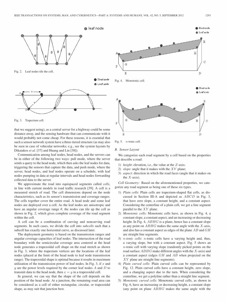
Fig. 3. Trapezium cell.

that we suggest using), as a central server for a highway could be somedistance away, and the sensing hardware that can communicate with itwould probably not come cheap. For these reasons, it is essential thatsuch a sensor network system have a three-tiered structure (as may alsobe seen in case of vehicular networks; e.g., see the system layouts byDikaiakos et al. [37] and Huang and Lin [38]).

Communication among leaf nodes, head nodes, and the servers canbe in either of the following two ways: pull mode, where the serversends a query to the head node, which then asks the leaf nodes for data,triggering the sensors that capture the data, and push mode, where theserver, head nodes, and leaf nodes operate on a schedule, with leafnodes pumping in data at regular intervals and head nodes forwardingcollected data to the server.

We approximate the road into equispaced segments called cells,in line with current models in road traffic research [39]. A cell is ameasured stretch of road. The cell dimensions depend on the nodecharacteristics, such as its sensor’s transmission and coverage ranges.The cells together cover the entire road. A head node and some leafnodes are deployed over a cell. As the leaf nodes are anisotropic andhave an angular coverage range θ, the nodes can tile up the cell asshown in Fig. 2, which gives complete coverage of the road segmentwithin the cell.

A cell can be a combination of curving and noncurving roadsegments. In such cases, we divide the cell into subcells such that asubcell has exactly one horizontal curve, as discussed later.

The deployment geometry is based on the transmission ranges andangular coverage capacities of leaf nodes. The intersection of the roadboundary with the semicircular coverage area centered at the headnode generates a trapezoidal cell shape on the road stretch as shownin Fig. 3, where the trapezium vertices are the locations of the leafnodes (placed at the limit of the head node to leaf node transmissionrange). The trapezoidal shape is optimal because it results in maximumutilization of the transmission power of leaf nodes. In Fig. 3, if x andy are the power levels required by the corner leaf nodes A and D totransmit data to the head node, then x = y in a trapezoidal cell.

In general, we can say that the shape of the cell depends on theposition of the head node. At a junction, the remaining road area canbe considered as a cell of either rectangular, circular, or trapezoidalshape, as may suit that junction best.

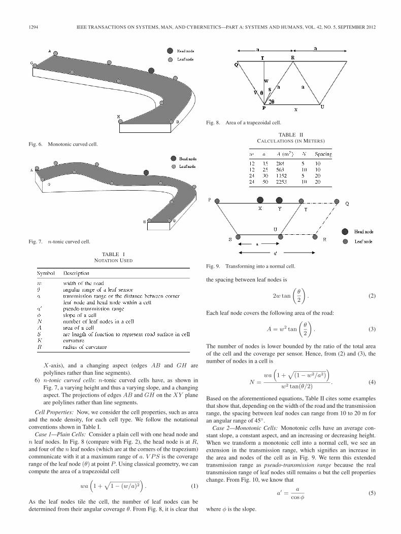
Fig. 4. Monotonic cell.

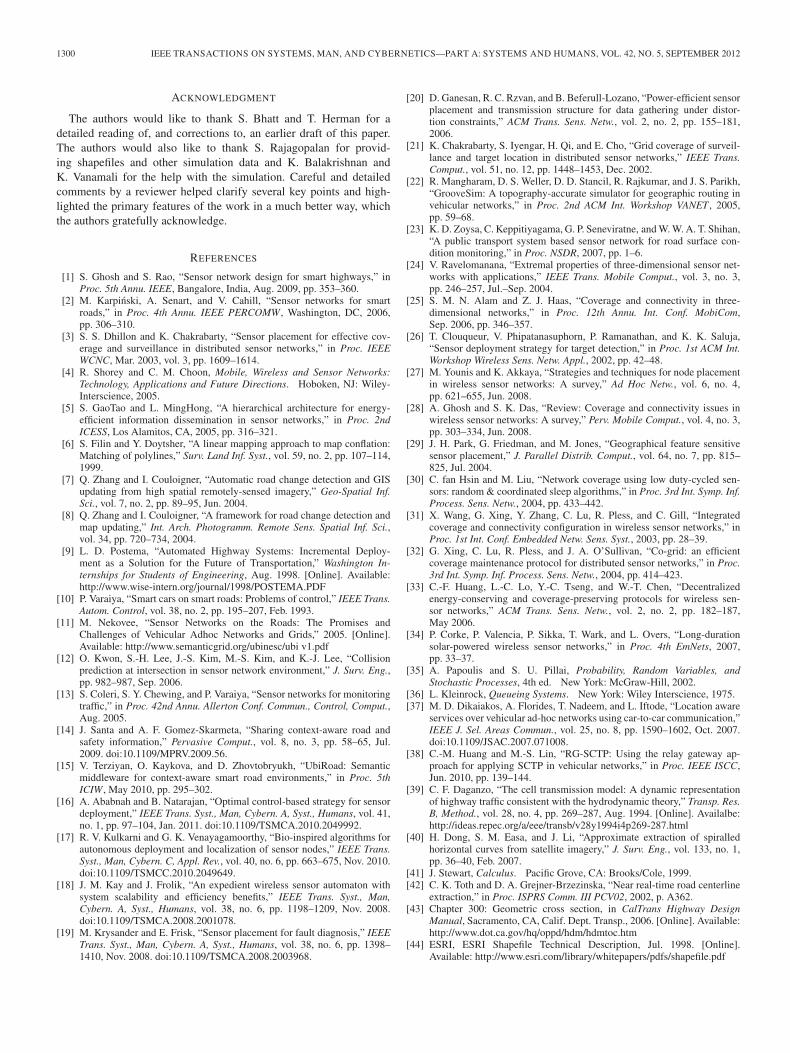
Fig. 5. n-tonic cell.

B. Sensor Layout

We categorize each road segment by a cell based on the propertiesthat describe a road:

1) height: elevation, i.e., the value at the Z-axis;2) slope: angle that it makes with the XY plane;3) aspect: direction in which the road faces (angle that it makes on

the X-axis).

Cell Geometry: Based on the aforementioned properties, we cate-gorize any road segment as being one of these six types.

1) Plain cells: Plain cells are trapezium-shaped flat cells, as dis-cussed in Section III-A and depicted as ABCD in Fig. 3,that have zero slope, a constant height, and a constant aspect.Considering the centerline of a plain cell, we get a line segmentparallel to the XY plane.

2) Monotonic cells: Monotonic cells have, as shown in Fig. 4, aconstant slope, a constant aspect, and an increasing or decreasingheight. In Fig. 4, ABHG is a plane, hence has a constant slopeas any point on ABHG makes the same angle with the X-axis,and also has a constant aspect as edges of the plane AB and GHare straight line segments.

3) n-tonic cells: n-tonic cells have a varying height and, thus,a varying slope, but with a constant aspect. Fig. 5 shows ann-tonic cell with varying slope (randomly picked points on theroad surface ABHG make different angles with the X-axis) anda constant aspect (edges GH and AB when projected on theXY plane are straight line segments).

4) Plain curved cells: Plain curved cells can be represented byFig. 12. Plain curved cells have a constant height, zero slope,and a changing aspect due to the turn. When considering thecenterline, we get a polyline rather than a straight line segment.

5) Monotonic curved cells: Monotonic curved cells, as shown inFig. 6, have an increasing or decreasing height, a constant slope(any point on plane ABHG makes the same angle with the


Fig. 6. Monotonic curved cell.

Fig. 7. n-tonic curved cell.

TABLE INOTATION USED

X-axis), and a changing aspect (edges AB and GH arepolylines rather than line segments).

6) n-tonic curved cells: n-tonic curved cells have, as shown inFig. 7, a varying height and thus a varying slope, and a changingaspect. The projections of edges AB and GH on the XY planeare polylines rather than line segments.

Cell Properties: Now, we consider the cell properties, such as areaand the node density, for each cell type. We follow the notationalconventions shown in Table I.

Case 1—Plain Cells: Consider a plain cell with one head node andn leaf nodes. In Fig. 8 (compare with Fig. 2), the head node is at R,and four of the n leaf nodes (which are at the corners of the trapezium)communicate with it at a maximum range of a. V PS is the coveragerange of the leaf node (θ) at point P . Using classical geometry, we cancompute the area of a trapezoidal cell

wa(1 +

√1− (w/a)2

). (1)

As the leaf nodes tile the cell, the number of leaf nodes can bedetermined from their angular coverage θ. From Fig. 8, it is clear that

Fig. 8. Area of a trapezoidal cell.

TABLE IICALCULATIONS (IN METERS)

Fig. 9. Transforming into a normal cell.

the spacing between leaf nodes is

2w tan

(θ

2

). (2)

Each leaf node covers the following area of the road:

A = w2 tan

(θ

2

). (3)

The number of nodes is lower bounded by the ratio of the total areaof the cell and the coverage per sensor. Hence, from (2) and (3), thenumber of nodes in a cell is

N =wa

(1 +

√(1− w2/a2)

)w2 tan(θ/2)

. (4)

Based on the aforementioned equations, Table II cites some examplesthat show that, depending on the width of the road and the transmissionrange, the spacing between leaf nodes can range from 10 to 20 m foran angular range of 45◦.

Case 2—Monotonic Cells: Monotonic cells have an average con-stant slope, a constant aspect, and an increasing or decreasing height.When we transform a monotonic cell into a normal cell, we see anextension in the transmission range, which signifies an increase inthe area and nodes of the cell as in Fig. 9. We term this extendedtransmission range as pseudo-transmission range because the realtransmission range of leaf nodes still remains a but the cell propertieschange. From Fig. 10, we know that

a′ =a

cosφ(5)

where φ is the slope.


Fig. 10. Monotonic cell.

TABLE IIICOMPARISON BETWEEN VARIOUS CATEGORIES

Fig. 11. Finding the arc length of a road surface.

Therefore, we modify (1) to find the area of 3-D cells as follows:

A = wa′(1 +

√1− (w/a′)2

). (6)

The area covered by the leaf node remains the same, as shown in(3), but N , the number of nodes in the cell, is now modified as givenbelow, compared to (4):

wa′(1 +

√1− (w/a′)2

)w2 tan(θ/2)

. (7)

See Table III for the area of a monotonic cell computed assumingthe width of the road w = 8 m, transmission range of leaf a = 25 m,and sensor coverage range θ = 45◦. Therefore, the area of the cell is455 m2, and the number of leaf nodes is 17, a 17% increase in the cellarea and a 13% increase in the number of nodes as compared to theplain cell. This means that the data processing and storage capabilitiesof head nodes must be 17% more in case of monotonic cells underthese conditions.

Case 3—n-Tonic Cells: n-tonic cells have fluctuating height, avarying slope, and a constant aspect. We consider the road surfacealong which vehicles are driven to be a function y = f(x). Wecompute the distance that the vehicle travels along the road in a cellfrom x = a to x = b. The horizontal distance covered is 2a, but thepseudo-transmission range a′ is half the arc length of f(x), S.

To find the arc length of a sample function y = f(x) in the interval[a, b], we approximate the function with a sequence of straight linesand add their lengths, as shown in Fig. 11. We break the interval[a, b] into smaller segments along the X-axis of width dx. When dx isinfinitesimal, the segment is approximated as a straight line. The length

of the hypotenuse ds is approximately the length along the curve forthe little segment. From Fig. 11, we have

ds =√

dx2 + dy2 =

√1 +

(dy

dx

)2

· dx (8)

where dy/dx is the slope of the segment. Also, dy/dx = f ′(x). Tofind the total length along the curve S, we integrate over the lengths ofall the segments

S =

∫ds =

a∫b

√1 + (f ′(x))2. (9)

For n-tonic cells, the range is from [0, 2a]. Hence, from (9), we get thearc length to be

S =

2a∫0

√1 + (f ′(x))2 (10)

a′ =S

2. (11)

The area and number of leaf nodes in an n-tonic cell can be derivedusing (6) and (7), respectively. Table III shows that, for w = 8 m,a = 25 m, θ = 45◦, and arc length S = 500 m, the area of the cellis 3999 m2, and the number of leaf nodes is 150, more than ten timesthat of a plain cell.

Case 4—Plain Curved Cells: Consider a car driving along a curvyroad. The tighter the curve, the more difficult the driving is apt to be.The curvature describes this tightness. If the curvature is zero, then thecurve looks like a line near this point. However, if the curvature value isnonzero, with no change in slope, such a curve is known as a horizontalcurve. A simple horizontal curve is a circular arc. Horizontal curvescan be of composite nature, like spirals which are composed of circulararcs, as discussed in [40].

Plain curved cells have a zero slope, a constant height, and achanging aspect. If its polyline representation is a function y = f(x)on the XY plane, the curvature of a function on the XY plane is givenby (12), the derivation of which can be seen in [41]

K(x) =|f ′′(x)|(

1 + (f ′(x))2)3/2 . (12)

The radius of curvature R is considered at the midpoint of thehorizontal curve and is represented as

R = K(a). (13)

As shown in Fig. 12, the length of the segment XY is 2a. If R be theradius of curvature, ρ that the angle XY makes with the center can becalculated as

sin(ρ

2

)=

2a

2R(14)

ρ =2 sin−1(a

R

). (15)

Therefore, the area A in case of a plain curved cell is

ρπ((

R+ w2

)2 − (R− w

2

)2)2π

= 2wR sin−1(a

R

). (16)

The number N of leaf nodes in the cell therefore is

2R sin−1(

aR

)w tan

(θ2

) . (17)


Fig. 12. Curved cell.

Fig. 13. Transformation of a monotonic curved cell into a plain curved cell.

The area and the number of nodes in a plain curved cell follow (16)and (17), respectively. Table III shows that the area and the number ofnodes in a plain curved cell are about 58 times those of a plain cellwhen w = 8 m, a = 25 m, θ = 45◦, and R = 200 m.

A cell can be a combination of one or more horizontal curves andnoncurving road segments. In such a case, we divide the cell into sub-cells such that each subcell has exactly one horizontal curve. Hence,twice the transmission range 2a in (14) should be substituted by thesegment length l of the horizontal curve in the subcell. Therefore,substituting 2a by l in (16) and (17), we have the area A of the subcellas follows:

2wR sin−1

(l

2R

). (18)

The number N of nodes in the subcells is

2R sin−1(l/2R)

w tan(θ/2). (19)

Multiple subcells within a cell can share a head node. If there is anobstruction between two consecutive subcells, each subcell can have adifferent head node in order to maintain connectivity with leaf nodes.

Case 5—Monotonic and n-Tonic Curved Cells: The road surface ina monotonic or n-tonic curved cell can be represented by functions inparametric form such that x = f(t), y = g(t), and z = h(t). For plaincurved cells, the height represented by z = h(t) is a constant.

Fig. 13 shows the transformation of a projected monotonic curvedcell on the XY plane into a plain curved cell. Although R remains thesame, the transmission range of the leaf nodes, i.e., 2a represented byLM , is extended to a pseudo-transmission range of 2a′ representedby PQ.

To derive the radius of curvature R, we consider the projectedhorizontal curve y = f(x) on the XY plane.

As we consider a simple horizontal curve, we need to transform itinto the equation of a circle

(x− h)2 + (y − k)2 = R2

where R is the radius of curvature and (h, k) is the center of the circle.The arc length S is given by∫ √

(f ′(t))2 + (g′(t))2 + (h′(t))2. (20)

Fig. 13 shows the projected transformation of an n-tonic curved cell(with the length of a segment of the horizontal curve being a) into aplain curved cell (of pseudo-transmission range a′), with the radius ofcurvature R remaining the same. a′ can be found as

S =Rρ = 2R sin−1

(a′

R

)

a′ =R sin(

S

2R

). (21)

From (21), we substitute the value of a in (16) and (17) as

A′ = 2wR sin−1

(a′

R

). (22)

The number N of nodes in the cell from (17) comes to

2R sin−1(a′/R)

w tan(θ/2). (23)

From the above equations, we calculate the area and the number ofnodes in the n-tonic curved cell. As shown in Table III, when w = 8 m,a = 25 m, and θ = 45◦, it is clear that there is an increase of about60% in the area of the cell and the number of leaf nodes comparedwith a corresponding plain curved cell.

If a cell consists of monotonic or n-tonic curved subcells withsegments to the horizontal curve of length l, then the area of the celland number of nodes in the cell can be given as

l′ =2R sin(

S

2R

)(24)

A′ =4wR sin−1

(l′

2R

)(25)

N ′ =4R sin−1(l′/2R)

w tan(θ/2).(26)

IV. SENSOR PLACEMENT STRATEGIES

This section introduces algorithms that form the strategies for de-ploying the leaf and head nodes on roads. As an input to the algorithms,the road is represented in one of its common representations, as apolyline, by considering its centerline. To begin with, we illustratethat there is an easy transition of a cell geometry to its polylinerepresentation and vice versa.

A. Polyline Representation of Cells

In this section, we show that a polyline is an appropriate representa-tion of a cell. It can also be used to find the actual cell shape as shownin Fig. 14.

We consider the road centerline to be represented by a polyline. Thecenterline extraction of roads can be done as by Toth and Grejner-Brzezinska [42]. We assume the road to be flat. The Highway Design


Fig. 14. Finding cell shape from polyline.

Manual of the California Department of Transportation [43] states that,for new construction, the slope should be 4:1 or flatter. This impliesthat, at every point on the road surface, when a cross section along thewidth of the road is taken, the height, aspect, and slope are constant.Therefore, a polyline which is the centerline of the road can be used torepresent the fluctuations in the height, slope, and aspect.

Let polyline AB = {(x1, y1, z1), (x2, y2, z2), . . . , (xn, yn, zn)}be the set of coordinates used to represent a cell on a road.

With known values of w and θ, we can find the cell shape and plottwo polylines along the sides of the cell.

1) Polyline PQ={(x1, y1−(w/2), z1), (x2, y2−(w/2), z2), . . .}.2) PolylineMN={(x1, y1+(w/2), z1), (x2, y2+(w/2), z2), . . .}.

From a tangent t1 at point A, we draw a line cutting the polylinePQ and making an ∠θ and cutting the polyline MN and making an∠(180◦ − θ).

At point B, we draw a line cutting polyline PQ making ∠θ withthe tangent t2 at point B and ∠(180◦ − θ) with the polyline MN .The resultant is the cell shape derived from the polyline.

From the polyline representation of a road, we may find the arclength, the pseudo-transmission range a′, and cell characteristics asmentioned in Section III-B.

B. Deployment

In this section, we introduce the algorithms for deploying the leafand head nodes on a road.

The first step in deploying the nodes is to divide the projectedpolyline into segments of equal length. Such a polyline segment is acenterline representation of a cell. We classify a segment as curvedor noncurved—if a road segment has a constant aspect, then it isnoncurving, and if it has a changing aspect, it is curving. Using thefunction representation of the cell, we compute the area of the cell andthe number of nodes within the cell. If the cell is not a plain cell, thenwe need a more powerful head node for that cell. As an alternative, wecan divide the cell into subcells equal in number to the ratio of the areaof the cell and the area of a corresponding plain cell.

Let D be a polyline representing the centerline of a road; D is anordered set of coordinate points or vertices. The edges are straight linesegments defined by consecutive pairs of points

D = {(x1, y1, z1), (x2, y2, z2), . . . , (xn, yn, zn)} .

The centerline of a road can also be represented by a set of polylinesegments T = {C1, C2, . . . , Cm}, where Ci is the ith polyline seg-ment of the road, given by an ordered set of coordinate points, such as

C1 = {(x1, y1, z1), (x2, y2, z2), . . . , (xr, yr, zr)}

C2 = {(xr+1, yr+1, zr+1), . . . , (xs, ys, zs)}

...

Cm = {(xt, yt, zt), . . . , (xn, yn, zn)}

where 1 < r < n, 1 < s < n, and 1 < t < n.

The X , Y , and Z coordinates for each of the cells are different. Thefirst vertex of the cell is considered to be the origin. The last vertex ofthe cell is the point on the polyline which intersects the X-axis at adistance 2a.

The functions used by the algorithms are as follows.

1) clip(startIndex,Y,m) returns a point on the polyline repre-sented by the set of coordinate points Y such that the differencein the X coordinate values of startIndex and the point returnedis of value m.

2) subset(startIndex, endIndex,Y) returns a subset of set Ywith elements starting from the startIndex ordinal value of Yuntil the element at the endIndex ordinal value of Y .

3) belongs(x,Y) returns TRUE only if x ∈ Y .4) low(Y) returns the lowest ordinal value (the first element) of a

set Y .5) high(Y) returns the highest ordinal value (the last element) of a

set Y .6) getV alue(i,Y) returns the ith ordinal value of a set Y .7) setV alue(i,Y, x) sets x as the ith ordinal value of a set Y .8) cardinality(Y) returns |Y|, the cardinality of a set Y .9) equals(a, b): If a ← (xa, ya, za) and b ← (xb, yb, zb), then the

function returns TRUE if xa = xb, ya = yb, and za = zb.10) index(x,Y): If x ∈ Y , this returns the ordinal value; else, it

returns −1.11) isNull(Y) returns TRUE if a set Y is the empty set.12) findRadiusCurvature(startIndex, endIndex,Ci) returns

the radius of curvature of the circular arc located from coordi-nates at startIndex to endIndex in cell Ci.

13) findArcLength(startIndex, endIndex,Ci) returns the ra-dius of curvature of the polyline located from coordinatesat startIndex to endIndex in cell Ci. Let x = f(t),y = g(t), and z = h(t) be the parametric form of equationsthat represent part of the polyline segment of Ci. Then,S ←

∫ √(f ′(t))2 + (g′(t))2 + (h′(t))2.

Algorithm IV.1 FRAGMENT_ROAD takes in D, the polyline repre-sentation of a road, as an input and fragments it into a set T of polylinesegments. It is based on the fact that any polyline representation ofcell Ci is a subset of D, i.e., Ci ⊂ D. In Algorithm IV.1, we generatesubsets of D where each of the subsets represents a single cell.

In Algorithm IV.1, we clip the road polyline of length 2a on Dstarting from the first vertex of the road polyline to get the end index.With the start and end indices, we represent the first cell by allottingthe coordinates of D from the start to the end indices to the cell. Inthe same way, other subsequent cells are represented. Thus, from theAlgorithm IV.1, we have m polyline segments of the road.

Let G be an ordered set of end points of the circular horizontalcurves on a road. If (a, b) ∈ G, then a is the starting vertex and b isthe end vertex of the circular horizontal curve. Also, G ⊂ D ×D.

We need to determine the circular horizontal curves particular to acell. If a curve extends to multiple cells, we need to split the curve andallot it to these respective cells. Let H be an ordered set of end points


of curves split according to cells. If (a, b) ∈ H , then a is the startingvertex, b is the end vertex of the circular horizontal curve, and both aand b are points in the same cell. Also, H ⊂ D ×D. Algorithm IV.2returns H , which is the set of cellwise circular curve end points.

In Algorithm IV.2, starting with (a, b) the first element in G and thefirst cell C1, if a and b are in the same cell, we add (a, b) to H . If not,we consider the next cell. If b lies in the next cell C2, we split (a, b)into two elements (a, high(C1)) and (low(C2), b) and add them toH . If b lies in the next cell C3, we split (a, b) into three elements(a, high(C1)), (low(C2), high(C2)), and (low(C3), b). Similarly,the other elements in G are examined to populate H .

To find if a road segment is curved, we use Algorithm IV.3. Fora given cell, we check if the elements of H are part of the cellcoordinates. Algorithm IV.3 takes in Ci, the ith polyline segmentof the road, as an input and returns h, an ordered set of curve endpoints present in the cell, where h ⊂ H . If the polyline segment isnoncurving, it returns a null set. Algorithm IV.3 is called as a routineby the main Algorithm IV.5.

In Algorithm IV.3, we create h, the ordered set of curve end pointsin the given cell Ci. For each set of coordinates in H , we compare itwith the cell coordinates and populate the set h in case the curve endpoints lie within the coordinates of the cell. If the cell is noncurving,the set h is an empty set.

Algorithm IV.4 is used to find the area of a curved cell. It is called asa routine by the main Algorithm IV.5. Algorithm IV.4 takes in a curvedcell Ci, the ith polyline segment, and returns the cumulative area ofthe subcells. Each of these could be curving or noncurving subcellssuch that each curved subcell is composed of a circular horizontalcurve.

TABLE IVRESOURCE ESTIMATION

Algorithm IV.4 takes Ci cell coordinates and h ordered sets of curveend points of Ci as input. Considering the first curve end points presentin the cell, we check if the starting vertex of the curve is the first vertex


TABLE VDEPLOYMENT PLAN: A SAMPLE OF A COMPLETE SET OF RECORDS

of the cell. If it is the first vertex of the cell, then we have a curvedsubcell and calculate the area for the subcell, and if not, we consider ita noncurving subcell and calculate the area of the same. Similarly, weconsider other curving or noncurving subcells of a curved cell and getthe cumulative area of the cell.

Algorithm IV.5 suggests a deployment scheme for each of thesegments, as described in Section III-B. It uses Algorithm IV.3 andAlgorithm IV.4. In Algorithm IV.5, for each of the cells, we calculatethe area of the cell and the number of leaf nodes in the cell. Then,we find the ratio of the computed number of leaf nodes with thenumber of leaf nodes in a plain cell. This ratio determines the needof dividing the cell into subcells or the need of a more powerfulhead node.

Algorithm IV.5 returns the value q, the ratio of the greater powerof the required head node as compared with the head node for acorresponding plain cell. An alternative would be to place one headnode at a distance of a. In both cases, we need to place N leaf nodesat a gap of 2w tan(θ/2).

C. Algorithm Performance

The algorithms have a computation complexity of the order oflength of the road, i.e., O(n). Algorithm IV.5, which provides thesensor layout of each cell, needs inputs from Algorithm IV.1, whichsegregates the road into cells. Algorithms IV.1 and IV.2 are prereq-uisites for Algorithm IV.5, but once the cell coordinates are known,Algorithm IV.5 can be parallelized.

V. URBAN GEOSPATIAL DATA

A geospatial digital vector storage format named a “shapefile,”specified by the Environmental Systems Research Institute [44], isa (mostly) open specification used to describe various spatial ge-ometries such as points, polylines, and polygons. For the purpose ofsimulation, we obtained spatial information for roads in the city ofBangalore, India, in shapefile format. We classified roads into two cate-gories, “Arterial” and “All” (this roughly agrees with the nomenclatureused by urban planners in India). “Arterial” roads are the roads withinthe city that are used the most, and “All” roads include Arterial roadsas well as other miscellaneous roads.

The estimation of resources required to build the system can berecorded as shown in Table IV, which shows consolidated informationabout the number of head nodes and leaf nodes to be deployed basedon the sensor placement strategy described here, for different roads(i.e., “Arterial” roads and “All” roads in Bangalore). The overall costto be incurred for this deployment can be estimated, which, in turn, canbe used to compare the costs incurred when the sensors are deployedrandomly and when the sensors are placed intelligently using theproposed sensor placement strategy.

We have assumed the amortized costs of a head node and a leafnode to be $2000 and $200, respectively. This estimate has been madeconsidering the approximate present-day costs of all the sensor motecomponents, the costs of labor to put together these components, andalso deployment costs. In other words, the costs of other equipmentincluding the servers and other support infrastructure are consideredto be amortized over the deployed head and leaf nodes only. Sincethe deployment costs involved can be known a priori, the roadsegments that are heavily used (i.e., “Arterial” roads) or those thatare accident prone can be given higher priority for wireless sensordeployment.

From the simulation results recorded in Table IV, it can be observedthat the ratio of the number of leaf nodes to head nodes for “Arterial”roads is much lower than that for other minor roads. The reason forthis is that the “Arterial” roads are generally well maintained andare more likely to require plain cells for the most part, while theother minor roads have many sharp turns and obstructions and aremore likely to require curved cells. Based on the cell architecturedescribed in Section III-A and the results recorded in Table III, weknow that, when a curved cell is transformed into a plain cell, due toan increase in the transmission range, the curved cell area covered bya leaf node is greater than the plain cell area covered by the same leafnode, and there is a need for more leaf nodes to be deployed for acurved cell.

The final deployment plan that can be used to place sensors on roadsis excerpted in Table V. It shows a sample of the list of all the subcellsalong with the information on the number of leaf nodes, the areacovered, and the distance between any two leaf nodes placed withina subcell. The coordinates of each road segment with the details of thenumber of sensors deployed in each of them can also be recorded.

VI. CONCLUSION

The motivation for this work arose from the fact that it is beyondquestion that sensor network technologies will find uses in highwayinfrastructures in the foreseeable future. However, the deploymentstrategy and architecture for such a sensor network system have nothitherto been explored in depth. Placement of sensor nodes usingrandom sprinkling is known not to be effective. This work thusconsiders a cell model similar to the ones used in studies of trafficflows and also takes into account the different types of cells, basedon the 3-D characteristics of road surfaces. Using basic trigonometricand geometric reasoning, we arrive at expressions for the number ofnodes required in each cell. This, in turn, gives rise to algorithmicstrategies that can be used for sensor placement. We validate this entireapproach by computing a deployment plan given real urban geospatialdata, which, in turn, leads to a simple cost estimate. This approach canbe followed fairly easily by urban planners, highway engineers, andsensor network designers anywhere.


ACKNOWLEDGMENT

The authors would like to thank S. Bhatt and T. Herman for adetailed reading of, and corrections to, an earlier draft of this paper.The authors would also like to thank S. Rajagopalan for provid-ing shapefiles and other simulation data and K. Balakrishnan andK. Vanamali for the help with the simulation. Careful and detailedcomments by a reviewer helped clarify several key points and high-lighted the primary features of the work in a much better way, whichthe authors gratefully acknowledge.

REFERENCES

[1] S. Ghosh and S. Rao, “Sensor network design for smart highways,” inProc. 5th Annu. IEEE, Bangalore, India, Aug. 2009, pp. 353–360.

[2] M. Karpinski, A. Senart, and V. Cahill, “Sensor networks for smartroads,” in Proc. 4th Annu. IEEE PERCOMW, Washington, DC, 2006,pp. 306–310.

[3] S. S. Dhillon and K. Chakrabarty, “Sensor placement for effective cov-erage and surveillance in distributed sensor networks,” in Proc. IEEEWCNC, Mar. 2003, vol. 3, pp. 1609–1614.

[4] R. Shorey and C. M. Choon, Mobile, Wireless and Sensor Networks:Technology, Applications and Future Directions. Hoboken, NJ: Wiley-Interscience, 2005.

[5] S. GaoTao and L. MingHong, “A hierarchical architecture for energy-efficient information dissemination in sensor networks,” in Proc. 2ndICESS, Los Alamitos, CA, 2005, pp. 316–321.

[6] S. Filin and Y. Doytsher, “A linear mapping approach to map conflation:Matching of polylines,” Surv. Land Inf. Syst., vol. 59, no. 2, pp. 107–114,1999.

[7] Q. Zhang and I. Couloigner, “Automatic road change detection and GISupdating from high spatial remotely-sensed imagery,” Geo-Spatial Inf.Sci., vol. 7, no. 2, pp. 89–95, Jun. 2004.

[8] Q. Zhang and I. Couloigner, “A framework for road change detection andmap updating,” Int. Arch. Photogramm. Remote Sens. Spatial Inf. Sci.,vol. 34, pp. 720–734, 2004.

[9] L. D. Postema, “Automated Highway Systems: Incremental Deploy-ment as a Solution for the Future of Transportation,” Washington In-ternships for Students of Engineering, Aug. 1998. [Online]. Available:http://www.wise-intern.org/journal/1998/POSTEMA.PDF

[10] P. Varaiya, “Smart cars on smart roads: Problems of control,” IEEE Trans.Autom. Control, vol. 38, no. 2, pp. 195–207, Feb. 1993.

[11] M. Nekovee, “Sensor Networks on the Roads: The Promises andChallenges of Vehicular Adhoc Networks and Grids,” 2005. [Online].Available: http://www.semanticgrid.org/ubinesc/ubi v1.pdf

[12] O. Kwon, S.-H. Lee, J.-S. Kim, M.-S. Kim, and K.-J. Lee, “Collisionprediction at intersection in sensor network environment,” J. Surv. Eng.,pp. 982–987, Sep. 2006.

[13] S. Coleri, S. Y. Chewing, and P. Varaiya, “Sensor networks for monitoringtraffic,” in Proc. 42nd Annu. Allerton Conf. Commun., Control, Comput.,Aug. 2005.

[14] J. Santa and A. F. Gomez-Skarmeta, “Sharing context-aware road andsafety information,” Pervasive Comput., vol. 8, no. 3, pp. 58–65, Jul.2009. doi:10.1109/MPRV.2009.56.

[15] V. Terziyan, O. Kaykova, and D. Zhovtobryukh, “UbiRoad: Semanticmiddleware for context-aware smart road environments,” in Proc. 5thICIW, May 2010, pp. 295–302.

[16] A. Ababnah and B. Natarajan, “Optimal control-based strategy for sensordeployment,” IEEE Trans. Syst., Man, Cybern. A, Syst., Humans, vol. 41,no. 1, pp. 97–104, Jan. 2011. doi:10.1109/TSMCA.2010.2049992.

[17] R. V. Kulkarni and G. K. Venayagamoorthy, “Bio-inspired algorithms forautonomous deployment and localization of sensor nodes,” IEEE Trans.Syst., Man, Cybern. C, Appl. Rev., vol. 40, no. 6, pp. 663–675, Nov. 2010.doi:10.1109/TSMCC.2010.2049649.

[18] J. M. Kay and J. Frolik, “An expedient wireless sensor automaton withsystem scalability and efficiency benefits,” IEEE Trans. Syst., Man,Cybern. A, Syst., Humans, vol. 38, no. 6, pp. 1198–1209, Nov. 2008.doi:10.1109/TSMCA.2008.2001078.

[19] M. Krysander and E. Frisk, “Sensor placement for fault diagnosis,” IEEETrans. Syst., Man, Cybern. A, Syst., Humans, vol. 38, no. 6, pp. 1398–1410, Nov. 2008. doi:10.1109/TSMCA.2008.2003968.

[20] D. Ganesan, R. C. Rzvan, and B. Beferull-Lozano, “Power-efficient sensorplacement and transmission structure for data gathering under distor-tion constraints,” ACM Trans. Sens. Netw., vol. 2, no. 2, pp. 155–181,2006.

[21] K. Chakrabarty, S. Iyengar, H. Qi, and E. Cho, “Grid coverage of surveil-lance and target location in distributed sensor networks,” IEEE Trans.Comput., vol. 51, no. 12, pp. 1448–1453, Dec. 2002.

[22] R. Mangharam, D. S. Weller, D. D. Stancil, R. Rajkumar, and J. S. Parikh,“GrooveSim: A topography-accurate simulator for geographic routing invehicular networks,” in Proc. 2nd ACM Int. Workshop VANET , 2005,pp. 59–68.

[23] K. D. Zoysa, C. Keppitiyagama, G. P. Seneviratne, and W. W. A. T. Shihan,“A public transport system based sensor network for road surface con-dition monitoring,” in Proc. NSDR, 2007, pp. 1–6.

[24] V. Ravelomanana, “Extremal properties of three-dimensional sensor net-works with applications,” IEEE Trans. Mobile Comput., vol. 3, no. 3,pp. 246–257, Jul.–Sep. 2004.

[25] S. M. N. Alam and Z. J. Haas, “Coverage and connectivity in three-dimensional networks,” in Proc. 12th Annu. Int. Conf. MobiCom,Sep. 2006, pp. 346–357.

[26] T. Clouqueur, V. Phipatanasuphorn, P. Ramanathan, and K. K. Saluja,“Sensor deployment strategy for target detection,” in Proc. 1st ACM Int.Workshop Wireless Sens. Netw. Appl., 2002, pp. 42–48.

[27] M. Younis and K. Akkaya, “Strategies and techniques for node placementin wireless sensor networks: A survey,” Ad Hoc Netw., vol. 6, no. 4,pp. 621–655, Jun. 2008.

[28] A. Ghosh and S. K. Das, “Review: Coverage and connectivity issues inwireless sensor networks: A survey,” Perv. Mobile Comput., vol. 4, no. 3,pp. 303–334, Jun. 2008.

[29] J. H. Park, G. Friedman, and M. Jones, “Geographical feature sensitivesensor placement,” J. Parallel Distrib. Comput., vol. 64, no. 7, pp. 815–825, Jul. 2004.

[30] C. fan Hsin and M. Liu, “Network coverage using low duty-cycled sen-sors: random & coordinated sleep algorithms,” in Proc. 3rd Int. Symp. Inf.Process. Sens. Netw., 2004, pp. 433–442.

[31] X. Wang, G. Xing, Y. Zhang, C. Lu, R. Pless, and C. Gill, “Integratedcoverage and connectivity configuration in wireless sensor networks,” inProc. 1st Int. Conf. Embedded Netw. Sens. Syst., 2003, pp. 28–39.

[32] G. Xing, C. Lu, R. Pless, and J. A. O’Sullivan, “Co-grid: an efficientcoverage maintenance protocol for distributed sensor networks,” in Proc.3rd Int. Symp. Inf. Process. Sens. Netw., 2004, pp. 414–423.

[33] C.-F. Huang, L.-C. Lo, Y.-C. Tseng, and W.-T. Chen, “Decentralizedenergy-conserving and coverage-preserving protocols for wireless sen-sor networks,” ACM Trans. Sens. Netw., vol. 2, no. 2, pp. 182–187,May 2006.

[34] P. Corke, P. Valencia, P. Sikka, T. Wark, and L. Overs, “Long-durationsolar-powered wireless sensor networks,” in Proc. 4th EmNets, 2007,pp. 33–37.

[35] A. Papoulis and S. U. Pillai, Probability, Random Variables, andStochastic Processes, 4th ed. New York: McGraw-Hill, 2002.

[36] L. Kleinrock, Queueing Systems. New York: Wiley Interscience, 1975.[37] M. D. Dikaiakos, A. Florides, T. Nadeem, and L. Iftode, “Location aware

services over vehicular ad-hoc networks using car-to-car communication,”IEEE J. Sel. Areas Commun., vol. 25, no. 8, pp. 1590–1602, Oct. 2007.doi:10.1109/JSAC.2007.071008.

[38] C.-M. Huang and M.-S. Lin, “RG-SCTP: Using the relay gateway ap-proach for applying SCTP in vehicular networks,” in Proc. IEEE ISCC,Jun. 2010, pp. 139–144.

[39] C. F. Daganzo, “The cell transmission model: A dynamic representationof highway traffic consistent with the hydrodynamic theory,” Transp. Res.B, Method., vol. 28, no. 4, pp. 269–287, Aug. 1994. [Online]. Availalbe:http://ideas.repec.org/a/eee/transb/v28y1994i4p269-287.html

[40] H. Dong, S. M. Easa, and J. Li, “Approximate extraction of spiralledhorizontal curves from satellite imagery,” J. Surv. Eng., vol. 133, no. 1,pp. 36–40, Feb. 2007.

[41] J. Stewart, Calculus. Pacific Grove, CA: Brooks/Cole, 1999.[42] C. K. Toth and D. A. Grejner-Brzezinska, “Near real-time road centerline

extraction,” in Proc. ISPRS Comm. III PCV02, 2002, p. A362.[43] Chapter 300: Geometric cross section, in CalTrans Highway Design

Manual, Sacramento, CA, Calif. Dept. Transp., 2006. [Online]. Available:http://www.dot.ca.gov/hq/oppd/hdm/hdmtoc.htm

[44] ESRI, ESRI Shapefile Technical Description, Jul. 1998. [Online].Available: http://www.esri.com/library/whitepapers/pdfs/shapefile.pdf

Documents

Sensor Network Design for Smart Highways