Embed Size (px)
Citation preview
Retrospective Theses and Dissertations Iowa State University Capstones, Theses and Dissertations
1-1-2003
Sensitivity analysis of combined travel demand / air pollution Sensitivity analysis of combined travel demand / air pollution
model for the Davenport area model for the Davenport area
Sheldon Andreu Harrison Iowa State University
Follow this and additional works at: https://lib.dr.iastate.edu/rtd
Recommended Citation Recommended Citation Harrison, Sheldon Andreu, "Sensitivity analysis of combined travel demand / air pollution model for the Davenport area" (2003). Retrospective Theses and Dissertations. 19985. https://lib.dr.iastate.edu/rtd/19985
This Thesis is brought to you for free and open access by the Iowa State University Capstones, Theses and Dissertations at Iowa State University Digital Repository. It has been accepted for inclusion in Retrospective Theses and Dissertations by an authorized administrator of Iowa State University Digital Repository. For more information, please contact [email protected].

Sensitivity analysis of combined travel demand /
air pollution model for the Davenport area
by
Sheldon Andreu Harrison
A thesis submitted to the graduate faculty
in partial fulfillment of the requirements for the degree of
MASTER OF SCIENCE
Major: Transportation
Program of Study Committee: Shauna Hallmark, Major Professor
Reginald R. Souleyrette David Plazak
Iowa State I~niversity
Ames, Iowa
2003

11
Graduate College
Iowa State University
This is to certify that the Master's thesis of
Sheldon Andreu Harrison
Has met the thesis requirements of Iowa State University
Signatures have been redacted for privacy

~~~
TABLE OF CONTENTS
CHAPTER 1. I~TTRGDI.TCTIOI~ 1
RATIONALE 1
PROBLEM STATEMENT AND SCOPE OF WORK 2
THESIS ORGANIZATION 3
CHAPTER ~. LITERATURE REV3EW A,ND C NT PRACTICE 5
EMISSIONS FACTOR MODELS . S
TRAVEL DEI~'LAND MODELING 6
Trip Generation $
Trip Distribution 9
Mode Split 12
Traffic Assignment 12
DATA NEEDS - 14
DATA COLLECTION METHODS FOR MODELS 1 S
DYNAMIC FEEDBACK LOOPING 17
CALIBRATION AND VALIDATION OF TRAVEL DEMAND MODELS ~ 8
Issues in Model Calibration 18
Issues in Model Validation and Reasonableness 20
SUGGESTIONS FOR IMPROVED MODELING PRACTICE 21
ALTERNATIVE MODELING APPROACHES 23
CHAPTER 3. DES CRIPTIO~T QF PILUT STUDY AREA 26
B I-STATE TRIP GENERATION DATA 26
B I-STATE TRIP DISTRIBUTION t~ICTION FACTORS) 28
CHAPTER 4. CALIBRATING TRANSCAD MODEL WITH BISTATE TRA►NPLAN
1VIODEL 29
CONVERTING TRANPLAN FILES 30
FORMATTING THE CONVER'1'ED INPUTS FOR TR.ANSCAD MODELING 34
THE FOUR S'~'~P TRAVEL DEMAND PROCESS 35
Skimming the Network (Shortest Paths) 36
Distributing the Trips 37

~~
Origin !Destination 39
Traffic Assignment 40
FEEDBACK LOOPING ~ 41
COMPARING 1998 ASSIGNED RESULTS 44
COMPARING 2025 ASSIGNED RESULTS ~6
+CHAPTER 5. PERPOR1ViING SENSITIViT~ RL~IS ON TRANSCAD MODEL 49
SENSITIVITY ANALYSIS 49
SENSITIVITY TESTING PROCEDURE 50
FRICTION FACTOR DISTRIBUTIONS 52
Friction Distribution 1 52
Friction Distribution 2 53
Friction Distribution 3 53
EFFECT OF VOLUME ON TRAVEL TIMES IMPACT OF FEEDBACK MODELING) 55
TRAFFIC ASSIGNMENT METHODOLOGIES 57
CHAPTER 6. LINKING TRAVEL MODEL OUTPUT WITH EMISSIONS RESULTS
60
MOBILE 6 EMISSIONS FACTOR MODEL 60
CHAPTER 7. ~:ES ULTS ~ .. 6 8
CI[APTER 8. ANALYSIS OF RESULTS 85
STATISTICAL ANOVA 85
ANOVA ANALYSIS OF INPUTS ~ 86
AI~IOVA Assumptions 86
E~:AMINING THE FRICTIONIFEEDBACK INTERACTION Err~CT 90
E~:AMINING THE INDIVIDUAL INPUT FACTORS _ 92
DISCUSSION OF INPUT FACTOR EFFECTS 96
Friction Factor Distribution 96
D~nan~ic Modeling 97
Assignment Technique Used _ 97
THE EFFECT OF SEASON ON POLLUTA►.NT EMISSIONS 98
S U~VIMARY 100
C~IAPTER 9. CONCLUSIONS 101

INPt.TT FACTOR SIGNIFICANCE A►ND CONSEQUENCES FOR EMISSIONS MODELING 101
Friction Factor Distribution 101
Dynamic Modeling 102 Assignment Technique 102
SEASONAL VARIATI{~NS 102 Carbon Monoxide 103 Nitrogen Oxides and volatile Organic Compounds 103
MODEL APPROACH LIMITATIONS 103 FUTURE RESEARCH ~ 104
APPENDIX A. FRICTION FACTOR TABLES 106
APPENDIX B MOBILE6 INPUT FILES (F'REE~VAY AND ARTERIAL) .109 APPENDIX C VISUAL BASIC CODE A►ND PROGRAM SCREENS~IOT 116 APPENDIX D ILLUSTRATION OF MAPPED EMISSIONS OUTPUT FOR l s~ INPUT FACTOR COMBINATION 133 APPENDIX E SCREENLI~~TE R:MSD TABLES FOR 1998 AND 202 DATA 136 APPENDIX F LINK COMPARISON TABLES ~ 143 APPENDIX G BI-STATE MODEL FILES 1 ~~
REFERENCES 156

V1
ACKOWLEDGEMENTS
I would like to thank the members of my committee, Mr. David Plazak, Dr. Reginald
Souleyrette and my major professor Dr. Shauna Hallmark for the invaluable advice and
guidance provided to me in preparing this thesis. I would also like to thank Mr. Lalit Patel of
the B i-State Regional Commission for his patience and advice in helping me convert the B i-
State TRANPLAN model to TransCAD. without his help, I can safely say, the thesis could
not have been completed.
To the staff and students at CTRE (Center for Transportation Research and
Education), your interest and motivational conversations were invaluable. Thank you
supervisor Dan Gieseman for the depth of advice related to your experiences going through
_ the same Master's degree process in which I am now involved. Thank you as well for the
Visual Basic help rendered that allowed me to automate part of the thesis work. On that same
note, thank you to fellow "Pit" members Brian Fiscus and Chris Gunsauluz for your VB
advice.
Dave V eneziano, Jamie Luedtke, Debbie Vitt, S itans u Pattnaik, Turhan Yerdelen,
Kevin Triggs, Jonathan Reese and all the other CTRE student members with whom I
interacted, your constant motivation and encouragement when I was under the most stress
particularly for my defense was greatly appreciated.
Finally to my mother, father, sister and other close family members and friends
scattered in several countries, thank you for your encouragement and constant checking up
on my progress. That helped provide me with the discipline to persevere particularly at the
times I needed it most. To all others who helped in their own little way not previously
acknowledged, "Thank You",

1
CHAPTER 1. INTRODUCTION
RATIONALE Air pollution is a major concern in many urban areas. it is defined as the
contamination of air by the discharge of harmful substances. (1) It is usually concentrated in
areas where significant industrial activity and vehicular travel occur. Air pollution produces
two main undesirable effects. First, it has major health effects, particularly for more sensitive
members of the population, such as children and the elderly. Particulate pollution from all
sources is estimated to cause 65,000 deaths annually (2) surpassing deaths from auto
accidents by a wide margin. Second, it is responsible for a number of undesirable
environmental effects such as acid rain, reduced visibility, crop damage, and global warming.
Given this situation, it is important to know exactly which pollutants are being
emitted, where are they emitted and in what quantity they are emitted. To accomplish this, it
is necessary to model air pollution. The sole emissions of interest in this thesis are mobile
source {on-road) emissions, which are responsible for nearly two-thirds of the carbon
monoxide, a third of the nitrogen oxides, and a quarter of the hydrocarbons emitted in the
atmosphere from anthropogenic sources. (3, 4, 5)
Over the last twenty years, emissions from mobile sources have decreased following
introduction of new technology to automobiles and trucks such as catalytic converters, EGR
(Exhaust Gas Recirculation), and unleaded and lower sulphur content fuels. However, the
vMTs (vehicle Miles Traveled) have been constantly increasing threatening to overtake
technological improvements. This negative trend is forecasted to accelerate in the future as
emissions control technology reaches a plateau while VMTs continue to increase.
Currently, on-road mobile source emission modeling is carried out in urban areas that
are classified as being in non-attainment for one of the transportation-related criteria
pollutants specified in the National Ambient Air Quality Standards (NAAQs) set forth in the
Clean Air Act Amendments. Areas are required to use modeling to evaluate impacts of
transportation projects and demonstrate progress towards conformity. Carbon monoxide
(CO), hydrocarbons (HC), and oxides of nitrogen (NOx) are the three criteria pollutants
typically modeled for on-road mobile sources. On road mobile source emissions modeling
for estimates of current or future emissions involves multiplying emission rates by vehicle

2
activity estimates. Emission rates are usually developed using the U.S. EPA's MOBILE
series of models. 'vehicle activity data in the form of vMT is obtained either from HPMS
{Highway Performance Monitoring System) or from travel demand forecasting model output.
Future scenarios are usually modeled using travel demand models.
Most urban areas in non-attainment are typically large metropolitan areas. Large
urban areas have collected data and calibrated and fine-tuned their travel demand models
over time to meet emissions modeling and planning requirements. I-Iowever, new air quality
standards are in the process of implementation and may affect smaller urban areas that may
not be as well equipped to handle modeling requirements. New eight-hour ozone standards
will take effect in late 20fl3 after finalization of the implementation rule. The original rule
was finalized in 1997 but implementation was delayed by numerous court challenges in the
proceeding years. These challenges have now been resolved. New PM2,5 transport rules are in
place and are about two years behind the ozone rules for implementation with finalization not
expected until 2006. (6) PM2.~ refers to particulate matter 2.5 microns in diameter or smaller
and includes fuel particles, dust etc. Similarly PMIo refers to particulate matter 10 microns or
less in diameter. Small and medium sized communities are expected to be impacted by the
regulations as well as large urban areas. Small communities frequently do not have well-
developed travel demand models and may lack the resources to collect and develop
additional data to make better estimates as well as implement better modeling procedures to
meet air quality requirements.
PROBLEM STATEMENT AND SCOPE OF WORK
New air quality standards are expected to impact small and medium sized
communities who have not dealt with air quality problems in the past and may not have
adequate travel demand forecasting models in place to meet transportation air quality
modeling requirements. This research intends to assist smaller areas in developing travel
demand forecasting models by evaluating which model inputs most significantly affect
emissions so that resources can be targeted appropriately. This research evaluates how the
combined travel demand /emissions factor model reacts to changes in key inputs and
answers key questions including "Which input factors) is/are most responsible for the output

3
results?", "Are any of the input factors interacting?" and "How significant are the other
factors in the determination of the final emission results?".
A sensitivity analysis on different combinations of input factors used in the models
was selected as the best method to answer these questions. Travel demand model input that
may affect output and subsequently emissions, include socioeconomic characteristics of the
area such as household income, average household size, and number and types of
employment activity in the area. The travel demand portion of the model consists of a three
or four step process. {Dependent on the extent of use of alternative travel modes and hence
mode split). These steps include in order of processing, the trip generation step, the trip
distribution step, the mode split step -- (Optional) and finally, the traffic assignment step. A
major travel demand model input is the friction factor (defined as model weighting factors
used to describe the travel behavior with regard$ to trip time distribution in the area). Other
major inputs include the representation of the roadway network in the study area.
Information such as average vehicle link traversal speeds, peak roadway capacity,
directionality of the roadways (one way or bidirectional) and others are usually included in
the roadway network. For the emissions factor portion of the model, major inputs are average
speeds of network links and VMT output from the travel demand model (TDM), ambient
temperatures, VMT fleet mix, and elevation.
This research focused on three factors used in the travel demand forecasting model
that may affect vehicle speeds and vMT that are used as input to emissions models. They
include: friction factors, traffic assignment technique used, and the presence/absence of
dynamic feedback Looping. The factors were analyzed by multi-factor Analysis of Variance
ANOVA. All statistical analyses were conducted with the SPSS statistical software
application. Standard diagnostic analysis and confidence intervals using multi-pair analysis
methods like Tamhane were used to determine the significance of each set of factors.
THESIS ~RGANIZATIOI~
The thesis is organized into five main areas. Chapter 1 presented an overview;
Chapter 2 is a literature review of the current practices and issues involved in the emissions
modeling process. Additionally, a description of a promising alternative emissions modeling
approach, the TRANS IMS system of travel forecasting models is presented.

4
Chapter 3 is a short description of the study area. Among items discussed are the data
sources and procurement. A basic map of the major transportation and geographic features of
the area is included.
Chapter 4 is a step-by-step description of the process and tools used to convert the
data from B i-State TRANI'LAN® format to TransCADO format. Included in this chapter are
example screenshots of dialog boxes used to perform data conversion and manipulation, the
filenames that were manipulated etc. Also included is a comparison of the B i-State
TRANPLAN® results and the TransCADO results using simple statistical techniques. Visual
traffic assignment results for both scenarios are illustrated for emphasis.
Chapter 5 details the sensitivity testing procedure. A brief discussion of the principle
of sensitivity analysis is performed. Graphical illustrations of the different combinations of
input factors are presented. The methods used to change friction factor levels; to include
feedback looping and to change the traffic assignment technique are also presented.
Chapter 6 is a description of the process used to combine the assignment output from
TransCAD® with emissions factor output from MOBILES. Included in this description are
flowcharts illustrating the main algorithm used in a custom Visual Basic® program that
automates the entire combination process. The Visual BasicO code is illustrated in Appendix
C.
Chapter 7 includes the presentation of the overall emission results by input factor,
season and pollutant type. In addition, emission, speed and VMT results for specifically
selected links are also presented.
Chapter 8 contains the ANOVA statistical analysis of the input factor sensitivity.
Relevant graphs and tables are illustrated as appropriate to assist in determination. of the
conclusion. Analysis of seasonal pollutant variation is also performed in Chapter 6.
Chapter 9 presents the overall conclusions of the research. Limitations in the research
procedure used and recommendations for future research close out the chapter.

CHAPTER 2. LITERATURE REVIEW AND CURRENT PRACTICE
in general, conventional air quality modeling practice involves the use of a travel
demand model to obtain v1VIT and link speed. These data are then used in conjunction with
emissions factor models to estimate quantities of pollutants generated in the study area.
Average vehicle speed is used as an input to emission rate models. VMT is multiplied by
emission rates output by emission rate models. A description of the methods to calculate
emission rates and the travel demand forecasting process including model limitations is
presented in the following sections.
EMISSIONS FACTOR MODELS
The most corr~rnon model to estimate emission factors is EPA's MOBILE models or
in the case of California, the EMFAC model. The default values used by MOBILE were
developed by the EPA based on a standard 11 mile-drive cycle FTP-75 {Federal Test
Procedure). In this cycle, vehicles are placed on a chassis dynamometer with the exhaust
connected to Teflon bags from which emissions are measured and recorded. A driver follows
the exact test procedure, which represents the starting, accelerating, decelerating, constant
speeds, and idling that is usual of a typical urban trip. The cycle consists of three phases with
the first being for cold starts, the second being the hot stabilized portion and the last being
hot starts. In the hot start phase, the vehicle is shut down and allowed to soak for about 10
minutes and then the procedure followed during the cold start phase is repeated. A cold start
is defined as an engine start after a vehicle's engine has been shut down for at least an hour.
The hot stabilized portion is defined as that phase of the test after the vehicle's engine has
been running long enough to reach normal operating temperatures. A hot start is defined as
an engine startup after a brief shut down period thus preventing the engine temperature from
dropping to the levels of a cold start. For each phase, a separate Teflon bag is used to capture
the emissions and the results analyzed accordingly. The results from several vehicles classes
are then averaged to arrive at the default emission values used in MOB ILEA.
MOB ILE6 is the most current emission rate model available from the EPA.
MOBILEfi requires a number of input parameters to estimate emission rates including

average travel speeds, temperatures, vehicle mix, humidity, etc. By using averaged data,
these models are of little use in analyzing specific "micro scale" evaluation that requires
specific speed and acceleration rate information. {7~ The FTP-75 test in addition does not
accurately represent the real driver in an actual urban operating environment. It must also be
acknowledged that there are great differences in the operating environment for differing
urban areas that may negatively affect results. An example would be differences in
acceleration rates; percent time spent idling in traffic, air conditioning use and others.
Attempts have been made to modify the FTP-75 test to more accurately account for these
limitations. Another modeling approach to overcome such problems has been to use modal
emissions models that give more detailed emissions information, in some cases second by
second emissions by vehicle type. (8~ This allows highly variable transient emissions from
aggressive driving behavior {high accelerations and decelerations) to be captured.
TRAVEL DEMAND MODELING
As one of the prime components of the modeling strategy being pursued in the
research, it is necessary to describe the principles in some detail. Travel demand modeling
was first used in the 1950s by state highway agencies to determine the need for new roads. It
comprises afour-step sequence that eventually leads to an estimate of the vehicular activity
on a particular network link. The four main steps are illustrated on the right of the diagram on
page 7 and include:
• Trip Generation
• Trip Distribution
• Mode Split
~ Traffic Assignment
Before the 4-step process is applied a network model is created. To perform travel
demand modeling, data processing limitations dictate that the transportation network will
need to be simplified compared to the real network. Consequently, networks in the travel
demand model, represented as sets of nodes with connecting links, do not include all the
roadways in the area. Local roadways are typically not included and depending on the scope
and the area being modeled, some collectors may also not be included. The omitted local and

collector roadways are represented collectively as links to zone centroids and are referred t®
as centroid connectors. Traffic Analysis Zones or TAZ's are the basic geographic unit in
travel demand modeling. They represent the sources and destinations of trips within the
region. A zone centroid is defined by a single point in a TAZ that represents the center of
gravity of trip activity for the entire zone.
~tatn urea ccography :- Get link distances,
1111k t}'1?e5 etc..
1 Create nelwt~rk with Tr~lvcl TimclCost allcl Capacity Parametca~s
Skim. thenet~~~r3rk Create the- shortest ti►3ie
1I11~1Cd~111CC nl~ltrlX
` fis Gcneration - {~f~tarl 'grip Prc~ductioils {P) ailci A.iraclic~ns (1~)
glance the tuture F'-~ to eilsurc that total rar~al l~s = tc,t~ I r«nal As Y
Use new congested travel times from assignment as input for updating network impedances
Appl y the ~;ravit` m:~del :- Tri ' Distrib.zticll
Ct~nvei-t Future F`s-_^,s to Orrin
.add l~xtern,il Trips
~'~rfai-n3 "Traffic ~ ssigrin_~etlt
Evaluate ~~ssi~~lma~nt :-Arc results rea.5dn,~hle`?
Yes
~`Prc~~eed to Ana S~~i.te ~f modelin~~ pnc~cess (Emissio 3 Factcr)
Figure 2.1 Travel Demand Modeling Process
Traffic Analysis Zones are discrete geographic entities within the modeled region that
are set up such that their attributes are as homogenous as possible. Hence, geographic areas
with large variations in household population, businesses etc. will need more TAZs than
would be the case otherwise. The TAZ boundaries can be determined from existing census
boundaries or they can be specifically developed from the known land-use, socioeconomic

8
and transportation characteristics of the area. TAzs are the basic unit in travel demand
modeling and represent the areas of trip productions and attractions. It is important that the
network detail matches the detail of the defined zones. If zones are small, it implies that the
network should be detailed enough to represent connections between such zones. This may
necessitate using collector streets and some local streets in the model on occasion.
Trip Generation The purpose of trip generation is to determine the trip making capacity for the area.
This capacity is affected by variables such as the affluence of the inhabitants of the region;
the number of inhabitants; the number of commercial and industrial establishments in the
area; and the presence of extraordinary establishments such as airports, universities, military
bases and sporting stadiums (special generators). Trip Generation can be divided into two
distinct segments known as trip productions and trip attractions. Trip producers are the
sources of trips while trip attractors are the recipients of the trips. Each trip that takes place
involves both this source and recipient and is referred to as a trip generation. Trips are further
divided according to source of production and purpose. Examples include HBW (Home
Based Work), HBO (Home Based Other) and NHB (Non Home Based) trips. There can also
be truck trips, taxi trips and other miscellaneous specific trip types depending on the
modeling scenario present.
There are several methods used to calculate the total trip generation of a model. The
most commonly utilized are activity unit rates such as the ITE trip generation rates,
regression methods and cross-classification. In regression methods that are often used to
calculate trip attractions, the trip rates are determined by applying the input socioeconomic
and other variables to a regression equation. This equation is believed to represent an
accurate algebraic relationship between the trip rate and the variables used as inputs. The
regression equation can be locally developed for the area under study if specific local
information is available. In the absence of such information, it is necessary to use generalized
rates found for example in NCHRP 365 (National Cooperative Highway Research Program) table 7 (10) or the ITE trip generation handbook. An example of a regression equation is as
follows:
HBW Attraction = 1.45 *Total Employment in analysis area. (NCHRP 365 table 7)

9
Cross-Classification involves grouping the input factors into specific categories each
with a corresponding trip rate. This rate represents the rate that has been observed for similar
groups in other areas. As with regression, specific rates or general rates from NCHRP 3 65
and the ITE handbook can be utilized. Cross-classification is most commonly used to obtain
trip productions, particularly for home based trips. It is seen as more reliable than the
regression methods but requires more detailed information to obtain trip rates for each
category.
After the trip productions and attractions are determined and balanced (made to be
equal to correct differences between trip production and attraction results), trip distribution is
then performed.
Trip Distribution As opposed to trip generation where the task is to determine the number of trips
produced or attracted in the study area, the aim of trip distribution is to predict the destination
of the generated trips. This is critical to determine the likelihood of a particular link being
used during the assignment phase and thus the number of trips on each link. In trip
distribution, a matrix is created of the number of generated trips from a specific TAZ and
attracted to another TAZ. An example of such a matrix is illustrated.
~~ 2I 3I 4~ 5I 6~ 7I BI 9I _.
1 198.60 191.16 47.97 107.17 82.60 41.44 55.22 138.70 73.11 91_,,,,, 2 191.16 186.32 47.85 103.62 80.29 42.47 54.95 133.98 74.52 88 3 47.97 47.85 12.77 25.84 15.27 11.57 14.14 33.44 26.14 50 4 107.17 103.62 25.84 56.36 44.75 21.78 28.31 28.03 38.94 44 5 82.60 80.29 15.27 44.75 34.72 18.13 9.63 21.72 31.97 21 6 41.44 42.47 11.57 21.78 18.13 10.60 12.16 28.15 23.59 16 7 55.22 54.95 14.14 28.31 9.63 12.16 14.61 36.60 22.20 48 8 138.70 133.98 33.44 28.03 21.72 28.15 36.60 94.32 70.79 140 9 73.11 74.52 26.14 38.94 31.97 23.59 22.20 70.79 2855.16 78 10 91.56 88.87 50.88 44.69 21.72 16.51 48.33 140.51 78.36 161 11 18.01 17.52 6.78 8.39 7.01 3.07 5.99 18.19 25.75 39 12 31.43 32.72 10.72 14.83 9.55 4.91 7.25 24.87 46.84 37 13 48.33 47.55 30.46 13.97 10.19 13.26 32.91 52.51 123 14 1.39 1.58 0.61 0.65 0.47 0.42 0.54 1.30 3.33 2 15 106.45 103.69 10.89 51.41 18.80 8.51 18.31 28.25 28.61 18 16 45.15 44.13 6.30 24.45 10.29 5.80 7.50 17.34 27.03 18 17 143.64 139.22 14.90 59.04 25.60 11.46 31.32 38.88 38.69 42 18 37.97 38.58 5.94 19.82 10.44 5.29 10.84 16.07 34.96 15 19 170.77 154.16 22.40 45.56 40.67 15.89 32.33 59.18 76.17 54 20 110.73 106.13 14.41 29.54 26.43 10.06 20.51 3$.35 50.72 34 21 133.2$ 127.80 30.31 65.32 30.91 13.37 29.51 84.73 88.02 58 22 145.49 139.37 32.21 67.44 26.46 22.58 28.01 87.31 54.62 82 ~~ ~
Figure 2.2 TransCAD Matrix Example

lfl
The column and row numbers are TAZs whereas the matrix values represent the
number of trips between the TAZs. The row totals represent the total productions from a zone
whereas the column totals represent the total attractions to the zone. In trip distribution, two
techniques are commonly utilized. They are growth factor methods and the gravity method.
Gf the two, the gravity method is the more popular.
Growt~i ~ac~or met~iod
In the growth factor method, the procedure involves the application of a scaling factor
to an existing Production-Attraction matrix file that represents the current travel conditions of
the study area. This factor represents the amount by which the traffic is expected to increase
in the studied time frame. There are three major types of growth factor methods, each
differing in the manner in which the factor is applied. They are as follows:
• The L.Tniform Growth Factor method
• The S ingly Constrained Growth Factor method
• The Doubly Constrained Growth Factor method (Fratar)
In the uniform growth factor method, the assumption is that the entire area grows by
the same rate and thus the original P-A matrix is multiplied throughout by the factor. It is the
simplest of the growth factor methods to be implemented but requires the unrealistic
assumption that the all segments of the modeled area grow by the same value.
In the singly constrained method, a different growth rate can be applied to either the
forecast productions or attractions for each zone. This allows the use of specific l~nowledge
on the manner in which the zones are expected to grow to be utilized in the model. The
singly constrained growth factor method (production) is represented by the following
equation. (11 }
Source: Travel Demand Modeling with TransCAD 4.0 page 73.
Pi
T1~ _ • tip
it must be noted that P~
_ z
ti represents the production growth factor

11
where: Tl~ =forecasted flow from zone i to zone j
Pi =forecast productions for zone i
t,3 =the original flout from zone i to zone j .
In the Fratar method, both the productions and attractions are used to update the
original matrix as opposed to the singly constrained model where either the productions or
the attractions are used. In this case, an iterative procedure is used to balance the resulting
zonal productions and attractions after application of the growth factors. The Fratar method is
commonly used to distribute external trips in models owing to lack of information on
external trip productions) attractions. This renders use of the alternative gravity technique in
external trip distribution inapplicable. The corresponding equation for this technique is as
follOWS:
Tip = t~~ ~ al * b~.
Source: Travel Demand Modeling with TransCAD 4.0 page 76.
The Gravity Model
This method of performing trip distribution is the most popular. It accounts for the
impedance between the TAZ's in the model. The impedance can be the travel time between
zones, the cost of travel between zones or combinations of the two. The gravity model is
similar in principle to Newton's law of gravitation where it is assumed that the P-A activity
will be proportional to zone size and the impact of such P-As will diminish with increased
distance/travel time or cost between zones. It can be expressed by the relationship (10):
P~ • `~•.f ~~i) T;~ _ ~p z . f'~~j~ if constrained to productions
ti
Or
A.1 T;~ _ ~p Z . , f'(~~ if constrained to attractions
~f(di)
z
where: Tip =the forecasted flow produced by zone i and attracted to zone j .
P~ =the forecasted number of trips produced by zone i.

t2
A~ =the forecasted number of trips attracted to zone j.
d;~ =the impedance between zone i and zone j (time, cost or both).
f(d;~) =the friction factor between zone i and zone j.
The friction factor represents a weight that is put on the timeldistance {impedance)
between the zones. Closer distanceslshorter times are usually given higher weights. By this
method, it becomes possible to accurately describe the travel behavior for the modeled area.
If local knowledge indicates that a higher proportion of trips in the area are of short distance,
the friction factor weightings can be adjusted to represent that reality. Friction factors are
among the three input factors that are varied during the sensitivity analysis performed in this
research.
1Vlode Split
In the mode split phase, the proportions of trips by auto, transit, bicycle, pedestrian
etc. is determined. The most commonly utilized methods include multinomial logit models
that generate the probability that a person will use a particular mode in the total set of modes
available by comparing the utility of each mode. The utility of a mode refers to the ease of
use of that particular mode with respect to travel time, cost or both. The comparisons can be
made at either the aggregate or disaggregate {individual decision maker) levels. Another
method is the incremental logic method that compares one mode choice to an existing
situation and is used often to study the impacts of improvements to a particular mode choice.
Traffic Assignment
The final stage of the travel demand modeling section, traffic assignment places
originldestination trips from the trip distribution) mode split phase onto the actual network
links. Several techniques are utilized including the following:
1. All or Nothing
2. Capacity Restraint
3. User Equilibrium
4. Stochastic
5. Stochastic User Equilibrium

13
6. Incremental
In the All or Nothing approach, the traffic flows between origin-destination pairs are
assigned on the shortest network paths connecting the origin and destination. It assumes that
only a single path is used despite the existence of alternative paths. It also does not handle the
potential delaying effect of increased volume/capacity ratios.
The Capacity Restraint approach is an attempt to account for the volumelcapacity
delay effect by recalculating the link travel times in an iterative process. This process has the
tendency however to bounce back and forth with the loadings on some high volume links.
This renders the results unreliable and hence other volume delay assignment techniques have
superseded Capacity Restraint.
In the User Equilibrium technique, a mathematical relationship is set up where no
traveler can benefit from improved travel times by shifting routes. Avolume-delay
relationship similar to that for the Capacity Restraint technique is used to adjust link travel
times. If a certain proportion of travelers shift routes, the travel times may be adjusted such
that the route is no longer an attractive alternative.
In the Incremental Assignment technique, volumes are progressively loaded onto the
network in steps. The actual assignment is based on the All or Nothing technique but the
difference is that only a fraction of the total volume is assigned in each step, after which new
volume-delay travel times are calculated. After each step, the assigned volumes are
progressively reduced until all the volumes are assigned. In many instances, particularly
when numerous steps are used, the output resembles that of Equilibrium Assignment
mentioned earlier.
In Stochastic Assignment, a logit model is used to determine the probability that a
particular reasonable path will be utilized. This probability is calculated based on the travel
time and cost of using a particular path. Paths that are circuitous are not usually considered
reasonable. Stochastic Assignment attempts to overcome the unrealistic assumption of the
All or Nothing technique of only one possible path being used.
In Stochastic User Equilibrium, an attempt is made to combine the logit techniques in
pure Stochastic assignment with the User Equilibrium technique. It was developed in an
attempt to model the fact that travelers do not have perfect travel cost information that is an

~~
implicit assumption in the pure User Equilibrium approach. Thus, under Stochastic User
Equilibrium, even very unattractive routes will have some volume assigned compared with
the pure UE approach. This for instance might capture a scenario where a driver prefers a
longer route that bypasses a toll way despite the toll way path being much shorter. In such a
scenario under normal UE, such a route might not be predicted to be used at all because of
the extra travel tune.
DATA NEEDS
Before any modeling can proceed, a large quantity of data must be collected and
tested for validity. Such data includes the travel network of the modeled area, the projected
population of the area, projected land-use, projected economic conditions and other data.
Accurate regional population and economic forecasts are vital for modeling given the
fact that the resulting travel activity is directly related to such factors. Such information is
obtained from custom run population and econometric growth models or publicly available
data from metropolitan, regional, state or federal sources. Demographic models, Input-output
models, regional simulation models for demographic and economic change and detailed
studies of particular industries, population groups etc. are likely sources of such data.
Techniques used to predict growth can also be estimated by simply extrapolating past trends
though this technique carries some risk. Careful studies of the modeled area would need to be
undertaken to determine whether extrapolation is appropriate.
After the broad regional level population and employment estimates have been
obtained, it is necessary to allocate the estimates by zone in the region. There are two main
techniques for allocating totals by zone. (12) In the negotiated estimates technique, the
preparer's judgment and desires based on political realities is used ,when apportioning the
estimates. This technique is used to some extent in almost all jurisdictions at present. In this
technique, local plans and projections are the primary guide. Allocations can be either by an
initially agreed across the board percentage between jurisdictions or the allocations can be
via negotiations between local jurisdictions. In the mathematical model approach, formal
relationships between economic factors are defined and used to determine how estimates are
apportioned. This technique ignores political realities and institutional constraints in favor of

15
a strong market force approach. The mathematical model approach is not very popular at
present owing to being perceived as inaccurate. It is used in a minority of jurisdictions. (12j
Another important data input for travel models is the rate of vehicle ownership.
vehicle ownership models have been developed that take into account the income, household
size, number of licensed drivers, gender, labor force participation, housing type, accessibility
to transit and other variables to estimate number of vehicles per household. These data are
usually applied at the zonal level. From a cursory analysis of some of the variables
mentioned, it is clear that some are statistically correlated thus necessitating care in model
estimation and analysis .
DATA COLLECTION METHODS FOR MODELS
In any transportation modeling process, the first step involves collection of the
necessary travel and socioeconomic data. Several methods are used including U.S Census
Bureau information and travel surveys. In particular, the Summary Tape File 3 and the
PUMS (Public Use Microdata) samples provide detailed information on many household and
individual characteristics of relevance to transportation planning.
Several types of surveys are commonly carried out to gather information for the
estimation and calibration of travel models. They include household travel surveys,
commercial vehicle surveys, transit rider surveys and external cordon station surveys. (13) In
recent years, there has been more activity with workplace surveys that are better able to
provide data for calibration with regards to the trip attraction stage of modeling. Such data
can be hard to capture in a traditional household survey but are nonetheless important for
overall model calibration.
In the common household travel surveys, information is obtained on the trip activity
of individual household members. Several techniques can be applied to obtain such
information such as telephone interviews and mailed surveys. In both cases, the data
collection costs can be high. Consequently, in recent years there has been a tendency for
surveys to get smaller with sample sizes in the range of 1,500 to 2,500 households. Large
surveys are now only conducted in the largest of cities such as l~ew York, Los Angeles and
Minneapolis where surveys upwards of 10,000 households have been undertaken on
occasion. Recently, it has been suggested that instead of focusing on household trips, it is

16
more appropriate to study household activities. This focus, it is thought will lead to a more
accurate recording of the trips made because individuals easily forget trips made, especially
short trips. In contrast, activities tend to be well remembered and can then be used to deduce
the trips made to link the activities. increased accuracy will then directly translate into a more
useful travel model particularly where it is being used for emissions estimation. ~.
In transit on-board surveys, passengers on transit vehicles are surveyed primarily by
using short questionnaires to be completed by the rider. Other experimental techniques
include data collection by the use of laptop computers. In many cases, the results of transit
surveys have been combined with household results to enable greater calibration accuracy
particular in the case of small sample household surveys.
External station surveys attempt to capture information on trips that either do not
originate or terminate in the modeled area. This information is very valuable for a model
given that in some areas external trips can be a significant percentage of the total trips
traveling through the region. In external station surveying as with other surveying, several
techniques can be used to gather the information. In roadside interviews, vehicles are stopped
at the external station and drivers are interviewed. This method has the potential to quickly
provide reliable data and high response rates. The main disadvantages are the potential for
traffic delays and disruption and the need for coordination with many organizations,
primarily law enforcement. Other data collection methods include postcard handoutlmailback
surveys and license plate recording mailing surveys. These rely on the driver eventually
completing the survey at home and mailing in the results. The difference between them is the
manner in which the driver receives the survey material. For the postcard handout method,
the surveyor simply gives the driver the survey material whereas for the license plate
recording method, the license plate is used to match against vehicle registrations and mailing
the surveys to vehicle owners. In these methods, the response rate is lower than for roadside
interviews and there is also an issue of privacy in the case of the license plate method.
Other survey types normally used to gather data for travel modeling include
commercial vehicle surveys, stated preference surveys and longitudinal surveys. These
surveys are more difficult to implement than the surveys previously mentioned such as transit
rider and household surveys and thus are not as widely utilized. There have been attempts
such as in the Puget Sound area of 'Washington State to carry out longitudinal surveys where
a select sample of households is surveyed over time to determine the changes in travel
behavior as changes in transportation supply and socioeconomic conditions occur. As is the
case for all survey types, there are benefits and drawbacks with a major problem being
attrition bias. In this phenomenon, the number of respondents participating at later stages in
the survey program is Tess than at the start owing to program dropouts during the course of
the survey. This tendency will introduce an inherent bias into model estimation by focusing
on only the respondents who are inclined to see the survey through to the end. it is important
that this phenomenon is recognized and corrected in model estimation.
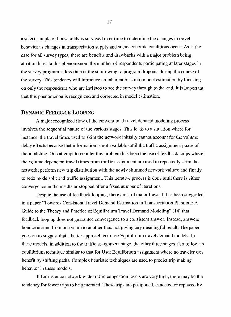
DYNAMIC FEEDBACK LOOPING A major recognized flaw of the conventional travel demand modeling process
involves the sequential nature of the various stages. This leads to a situation where for
instance, the travel tunes used to skim the network initially cannot account for the volume
delay effects because that information is not available until the traffic assignment phase of
the modeling. One attempt to counter this problem has been the use of feedback loops inhere
the volume dependent travel times from traffic assignment are used to repeatedly skim the
network; perform new trip distribution with the newly skimmed network values; and finally
to redo mode split and. traffic assignment. This iterative process is done until there is either
convergence in the results or stopped after a fixed number of iterations.
Despite the use of feedback looping, there are still major flaws. It has been suggested
in a paper "Towards Consistent Travel Demand Estimation in Transportation Planning: A
Guide to the Theory and Practice of Equilibrium Travel Demand Modeling" (14} that
feedback looping does not guarantee convergence to a consistent answer. Instead, answers
bounce around from one value to another thus not giving any meaningful result. The paper
goes on to suggest that a better approach is to use Equilibrium travel demand models. In
these models, in addition to the traffic assignment stage, the other three stages also follow an
equilibrium technique similar to that for User Equilibrium assignment where no traveler can
benefit by shifting paths. Complex heuristic techniques are used to predict trip making
behavior in these models.
If for instance network wide traffic congestion levels are very high, there may be the
tendency for fewer trips to be generated. These trips are postponed, canceled or replaced by

I8
teleconferencing etc. In a situation where congestion on specific links is a problem, the
tendency is for trips to be diverted to more accessible areas. In this instance, the results of the
trip distribution process will be altered, For the mode split example, if the travel costs on the
highway mode increases, there is the potential that some trips will be diverted to transit, ride
sharing etc. Complex heuristic procedures again automatically attempt to reestablish
equilibrium.
It is thought that equilibrium travel demand models, despite added computational
complexity are worth the effort. It overcomes one of the major flaws in the 4-step approach
by generating consistent, reliable estimates and it integrates aggregate travel demands with
discrete-choice theory in a consistent manner. It is also the first step to dynamic modeling as
attempted in activity based disaggregate models such as TRANSIMS®.
CALIBRATION AND VALIDATION OF TRAVEL DEMAND MODELS
Upon reviewing the available literature, it became apparent that among the primary
issues to be tackled in the modeling process being pursued is the actual usefulness of the
output from the travel demand model. It is of vital importance to calibrate the travel demand
model as much as possible to represent real-world conditions particularly since emission
rates are highly dependent on volume and speed estimates.
Calibration involves use of model inputs to determine model estimates. Following
accurate calibration, it then becomes necessary to check the reasonableness of the model
results by comparing to predicted outputs to actual outputs and subsequently fine-tuning
model variables until results with an acceptable range of error are obtained. This step is
referred to as Model Validation and Reasonableness.
Issues in 11~Iodel Calibration
Calibration refers to the task of modifying model input parameters until the output is
similar to observed travel behavior. ~ 15) This means that the results of the distribution
process, Origin-Destination matrixes are consistent with real trip Origin-Destination values.
On the emissions end, it is important that the correct vehicle operating mode classification,
VMT distribution, trip purpose, ambient temperature etc. are selected. These variables have

19
an important impact on the actual emissions output necessitating great care in their selection
and use.
The main parameters adjusted in calibration of travel demand models are
(i) Friction factors: -They determine how trips will be distributed and it is very
important to get factors that accurately describe the distribution of trips by trip
purpose. For example, changing the friction factor curves can adjust the average
length of trips either upwards or downwards and significantly change the trip
distribution results. It must be noted that the friction factors for different trip
purposes wi11 be different thus each trip purpose will have to be separately
calibrated.
(ii) Network parameters : -Parameters such as number of links, direction of flow on
the links, speed of the links, intrazonal travel times, turn restrictions and number
and placement of centroid connections from the link-node network to zone
centroids need to be accurately described. Results will be of little use, for instance
if a link that is in reality one-way flow is coded as having flow in the opposite
direction. Incorrectly defined link speeds can also affect the results of trip
distribution, as impedance values will be inaccurate.
(iii) Trip generation parameters such as socioeconomic variables like average
household size, CPI (Consumer Price Index), average auto occupancy in the
modeled area, household income and others need to be carefully evaluated to
ensure that they are up to date and relevant. Special Generators need to be applied
as appropriate to describe unconventional trip patterns.
(iv) The impact of truck trips, external trips and other non-standard trip types needs to
be carefully observed and integrated into the model.
For the assignment phase, it is important to account for the impact of volumes on trip
times. If the area being studied does not have high volumes, simple assignment procedures
such as the All or Nothing can produce acceptable results, otherwise a technique with volume
delay attributes like Equilibrium Assignment will be necessary. It should be noted that in
conventional practice, the most common assignment technique is the Equilibrium technique.

20
Issues in Model Validation and Reasonableness
Ideally, after each stage in the Travel Demand Modeling process, the output should
be checked for validity and reasonableness. This minimizes the scale of the errors that
inevitably propagate as the various stages in the TDM model are executed. Two main types
of validation tests include Reasonableness tests and Sensitivity tests. (16) The first category
of tests can include Absolute and Relative difference tests, Statistical correlation tests and
variance tests such as RMSE (Root Mean Square Error). The sensitivity tests check the
model behavior when inputs are varied.
1Vlodel Inputs and Trip generation
In this phase, it is necessary to check that the socioeconomic and land use data
actually being used for the model is accurate. Items to check for include population densities,
workers per household, vehicles per household among others. Transportation network entities
also need to be checked for such things as correct link alignments etc. In other words,
verification that the link and node network present in the model represents the real
transportation network for the study area is required.
Trip Distribution
The main validation check in trip distribution is the check for correct travel
impedances (i.e. Are the distances, speeds and consequent travel times in the network
representative of actual values. Statistical tests that compare distributions (coincidence ratios)
are used for to determine for example if observed and average trip lengths are significantly
different. This can quickly highlight problems that are occurring in the distribution phase
with the usual result being an adjustment of friction factors assuming the trip generation
phase validation errors were acceptable.
1Vlode Choice and Auto Occupancy
Typically, this validation usually involves sensitivity tests with known data from other regions for determination of appropriate model coefficients. For the auto occupancy
rates, comparisons with either generic socioeconomic or known local data using absolute
difference tests would suffice.

21
Traffic Assignment The main validation for this step involves comparing model outputs with observed
counts. The main test is a t-test to compare differences in means. Issues of relevance in
validation of traffic assignment include the type of link; i.e. whether it is major, medium or
minimal in terms of average daily traffic. Major links by necessity should have lower values
for error given that the consequences. for forecast errors on such links will be greater (greater
cost to add lanes, change geometry, traffic signaling etc.). Tables of acceptable error ranges
are usually referred to following this stage, A growing trend and also recommended practice
involves using feedback loops to alter the impedance inputs to the trip distribution phase
giving for example more realistic travel times. This in turn should produce more realistic
assignment results .
SUGGESTIONS FOR IMPROVED MODELING PRACTICE It has been recognized in a number of recent research papers and manuals such as the
"Manual Of Regional Transportation Modeling Practice for Air Quality Analysis" (12) that
most models have endured significant underinvestment for over 20 years. It is felt that for
present models to be more relevant and useful, existing gaps in input data such as detailed
land use and employment data; transit ridership patterns; up to date demographic information
etc. need to be corrected. Another major concern is the dearth of knowledge of trip timing
and trip chaining which in recent years has seen significant increases. Trip chaining is
described as the combination of several trips into one such as making a trip to perform
several errands . An example includes the trip home from work that includes stops at the
grocery store, child pick up from school and other miscellaneous stops. Trip chaining is not
handled very well in present models because of the need to stratify trips into rigid purposes.
Chained trips can have major implications for emissions output given that in many instances they are short thus necessitating more frequent engine starts.
Other issues mentioned in the manual include the ability of present regional models to
represent pedestrian, bicycle and other urban design transportation control measures. It has been suggested that land use impacts of transportation investments be determined and the
models adjusted accordingly if such impacts are indeed found to be significant.

22
Given these and other shortfalls, the manual suggests some areas that should be given
priority for improvements . They include the following items
• Accurate up to date travel surveys including household surveys, transit surveys etc.
are vital to ensure that the best available information is used to develop model
estimates. In addition to the standard information such as household income, size and
auto availability, other key variables to be garnered include number of school aged
children, number of workers, transit accessibility and type of housing unit. These
additional variables have a key influence on the trip production rate of the household,
particularly by trip type. (12)
• Accurate V1VIT information is required. This will necessitate increased traffic counts.
It is also important pursue accurate speed monitoring which will be of great
importance in air quality estimation. { 12)
• It has been suggested that more trip purposes should be used. This will allow a better
representation of the more complex trip patterns commonly observed in contemporary
trip making. Examples include school trips, shopping trips, sporting event trips,
miscellaneous errand trips etc. Trip chaining will be better represented under this
scenario. (12)
• It is important to have as detailed a highway network as practicable representing all
roadways carrying significant interzonal traffic. Networks of 2,Oo0 or more links
have been feasible for the last decade owing to increased computer processing power.
As processor power increases in the future, maximum advantage should be taken to
improve model detail.
• For modeling bicycle, pedestrian and other non-motorized trips, calculations should
be performed separate from the model by hand if necessary and the results integrated
at a later stage. V~hile not the perfect solution, it is nonetheless a better strategy than
to completely ignore such modes if they represent significant modal shares. (12)
• 1V~ore realistic assumptions are needed. For instance, the assumption in many current
models that vehicle speeds do not exceed the legal speed limit is not acceptable. This
introduces inaccuracies in the travel forecasts and consequent emissions estimates.
(l 2) For freeways, such assumptions could have a negative impact on emissions
estimates whereas for arterials, the converse may be true.

23
• It has been suggested that transportation control measure TCM effectiveness can be
used to improve analysis capabilities. For instance, TCM effectiveness found from
before and after studies could be used to determine if calibrated model parameters are
actually representative.
• Finally, present models are acknowledged to have poor documentation. (12j This
makes it difficult for model improvements to be implemented. In addition, lack of
sufficient documentation makes it very difficult for trends monitoring and repeat
analysis. It is thus suggested that documentation be improved particularly on
documentation describing how the model functions. Over the long run, it is thought
that extensive documentation will actually lead to reduced expenditures and more
easily improved models that are able to respond to fast changing inputs.
ALTERNATIVE MODELING APPROACHES
In recent years, there have been attempts to employ a completely different process for
travel model/emissions estimation. One such approach has been the use of activity based
travel models combined with emissions models that have modal characteristics. Known as
TRANSIMS (Transportation Analysis SIMulation System), this approach contains
significant differences from the traditional travel demand emissions factor model approach.
TRANSIMS is an integrated system of travel forecasting models designed to give
transportation planners accurate, complete information on traffic impacts, congestion, and
pollution (17). It differs from the traditional approach by attempting to model the individual
traveler in the system as opposed to an aggregation of behaviors of travelers in a zone (TAZ).
It is hoped that modeling on the disaggregate level will provide more accurate results given
the ability to explicitly model individual traveler characteristics, activities and their
interactions with the transportation system.
As opposed to the four-step process combined with vehicle activity estimates in the
traditional process, TRANSIMS consists of a Framework that includes several sub modules
as follows:
~ Population Synthesizer
• Activity Generator
• Route Planner

24
• Traffic Microsimulator
• Selector/Iteration Database
• Emissions Estimator
• Output Visualizer
The Population Synthesizer module is used to generate a virtual population of all the
individuals in the region under study. Data sources, as in the case of the traditional modeling
approach include IJ.S Census Bureau population information, population projection
information and geographic correspondence engines to link the related population
geographically. Aseries of algorithms is performed to convert the census information to
discrete individual travelers in the model.
Once each population member has been generated, the Activity Generator is used to
compile a list of activities that such members will partake in. The demographics of the
population will be used to determine the types of activities selected. For each activity, its
type, time frame, preferred transportation mode, location and other possible participants are
noted. Survey data from actual households is used to estimate likely activities in the model.
Once the attributes for each activity is accurately captured, it then becomes possible to model
trips by mode, length etc. Information such as travel time from the Route Planner and Traffic
Microsimulator is fed back to this stage and used to help determine activity locations. The Route Planner is then used after travel activities have triggered trip requests to
determine the actual travel routes for each traveler in the model. Trip requests consist of an origin and destination, the time frame in which the trip is to be completed and the mode choice to be used for the trip. The trip request information along with the TRANSIMS network information, traveler information etc. is then used to determine a shortest path route similar to that of network skimming in the traditional TDM process . This shortest path is time dependent and thus could be negatively affected by delays. To accommodate such a situation, a mechanism for feedback from the Traffic Microsimulator is available.
The Traffic Microsimulator attempts to simulate the movements of all the individual travelers in the system including the effects of their interactions. The main input is the trip plan produced by the Route Planner for each traveler. Detailed algorithms are used to simulate the interactions between each traveler and the modes they utilize. The Traffic Microsimulator allows for the modeling of walking stages in addition to transit and car stages thus representing a big improvement over the traditional process. The output from the Traffic

25
Microsimulator consists of spatial and temporal summary data, traveler events and snapshot data that allows for traffic animation. (18)
The Selector/Iteration Databases module is used to implement the iterative feedback process that is critical to model accuracy. With this module, it is possible to use optimized travel times for instance in activity location. It is also possible to use this module to select particular types of travelers for detailed analysis or to direct the travelers to certain choices known to occur in the region. This module can thus be thought of as a way to tweak the overall- model without having to redefine the entire model. (1$)
The Emissions Estimator uses information from the Population Synthesizer regarding vehicle population and the output from the Traffic 1Vlicrosimulator to generate emissions estimates. The vehicle type, speed, age and operating mode and other data similar to that used in the Emissions Factor stage of traditional modeling is used. with the travel output from TRANSIMS at a disaggregate level, it is possible to determine vehicle operating mode, speed, age etc. far more precisely thus leading hopefully to more accurate emissions estimates than is the case in the traditional process. {18)
Finally, the Output Visualizer enables various input and output data sets to be displayed. This facilitates easy analysis of the overall model and can be regarded as a model management tool. { 18)
It is hoped that this new activity based disaggregate approach to transportation modeling will provide a significant improvement over the traditional process. Nevertheless, high data processing needs will for the foreseeable future limit application to only those metropolitan areas provided with sufficient resources, For instance, parallel computer processing using multiple computers and other expensive hardware is required to model a city of greater than 1 million at an individual level. The data input needs are also formidable thus necessitating costly detailed surveys.

26
CHAPTER 3. DESCRIPTION OF PILOT STUDY AREA
As stated in Chapter 2, high input data accuracy in travel modeling is desired. In
addition, the models should be well calibrated and validated. The travel demand model inputs
and calibrated parameters developed for the Quad Cities area of Davenport, Moline,
Bettendorf and Rock Island in the states of Iowa and Illinois was selected for the pilot study
area. This model incorporated dynamic distribution that theoretically should result in a better
calibrated model. Additionally, the effect of dynamic distribution is among the major areas of
research in this thesis, hence the Bi-State model served as a useful model on which to
perform the research.
The Bi-State Regional Commission is an agency responsible for transportation
planning in the Quad-Cities region of Iowa and Illinois. It is an organization of five Iowa and
Illinois counties and 44 municipalities including the cities mentioned previously. This region
is comprised of a population of approximately 300,000 located about midway between the
midwestern cities of St. Louis, Minneapolis, Chicago and Des Moines. The Mississippi River
bisects the region in a general Northeast to Southwest direction. Interstates 80, 74 and 280,
each of which has a Mississippi River crossing, serve the area. The busiest crossing had a
January 2001 ADT (Annual Daily Traffic) count of just over 70,000 vehicles while the
freeways in the area carry between 15,000 and 40,000 vehicles per day. { 19)
BI-STATE TRIP GENERATIQN DATA Originally to develop the model, the Bi-State Commission in cooperation with the
Iowa DOT used a program called PLANPAC. PLANPAC was a mainframe computer
software package and was used before 1992 when an exponential increase in electronic
processing power enabled personal computer based modeling applications. Further updates
have been made to the original TAZs to reflect changes in socioeconomic conditions, land
use and consequent urban travel activity.
Data such as the number of housing starts, population per square mile by TAZ,
manufacturing, service and retail employment levels were used to estimate future trends.
These trends were then converted using trip generation analysis to forecasted trip activity by
TAZ. Population data were obtained in the 1998 base case from updated 1990 census block

~~
level data. Data including employment per residence, place of work, school enrollment and
school age population obtained from census 1990 data; Iowa Department of Employment
Services; and Illinois Department of Employment Security were used in trip generation.
Population forecasts for the 2025 year were projected in a straight line fashion based on
historical trends in the Quad Cities area. It is projected in the model that a net population
increase of 19°10 will occur between the 1998 and 205 years.
Figure 3.1 Basic Transportation Map of Study Area taken from Broadway Historic District Website. (36)
Employment forecasts were determined by calculating a ratio of employment per
capita in each county for 1998 data. For the Iowa cities, the ratio was found to be 0.54
whereas the value for the Illinois cities was 0.51. These ratios were then extrapolated to the
year 2025 using 2025 population values to obtain employment values.
Following the acquisition of population, employment, school data etc., the Bi-State
Commission used initial trip rates from Des Moines MPO. Des Moines is regarded as
possessing similar population and transportation infrastructure as the Quad Cities area.

28
Adjustments were then made to the resulting trip rates to accommodate the specific
differences between the Quad Cities area and Des Moines. The rates were adjusted in
accordance with the NCHRP Report 187 (Quick-Response Urban Travel Estimation
Techniques and Transferable Parameters) parameters. The Cross-Classification trip
generation technique was also used in the trip rate adjustment. Truck trips or Internal
Commercial Vehicle trips were calculated using an equation utilized by the Des Moines
MPO given that no specific truck data was available for the Quad Cities area.
BI-STATE TRIP DISTRIBUTION (FRICTION FACTORS) Friction factors were developed from a travel time study performed in 1998. The
study was performed primarily on major arterials in the Quad Cities at the request of city
traffic engineers. Both the AM (morning) peak and the PM (evening) peak were included.
Each trip type was individually calibrated to produce acceptable trip distribution results
following an iterative process.

z9
CHAPTER 4. CALIBRATING TRANSCAD MODEL WITH BISTATE TRANPLAN MODEL
Several tools are available to perform conventional travel demand analysis. Among
the more popular are TRANPLAN®, TransCADC~, QRS II and MINLJTP. Each tool tends to
have different features and strengths. TRANPLANO for instance is valued for its flexibility
and power; QRSII for its user friendliness and TransCADfl for its tight integration of GIS
functionality with traditional travel modeling functionality. For the purposes of this thesis
research, the two tools of interest are TRANPLAN® and TransCADO.
The original Bi-State travel model used for the pilot study was implemented using
TRANPLAN®. TRANPLANO is a command line FGRTRAN based set of integrated
programs for the transportation planning process. (20) As with ail other travel demand
modeling software, it allows all four stages of the four step process to be implemented.
Output from TRANPLAN® is a text or binary output file representing the network with
loaded volumes and travel tunes. Despite being an older travel demand modeling application,
TRANPLANC~ remains a widely used application. Compared to other travel demand
modeling applications, it provides powerful and flexible travel demand modeling capabilities.
Although the Bi-State model was originally available in TRANPLAN format,
TRANSCAD® was selected as the platform to complete the 4-step model and sensitivity
analysis since TRANSCADO provides the best GIS functionality of all the tools used in
conventional travel demand planning and was most familiar. TRANSCADO is a GIS based
travel demand forecasting software tool developed by Caliper Corp. in Massachusetts.
Common functions such as polygon overlay analysis, buffers and geocoding are all notable
GIS features. In addition, transportation specific functionality such as networks, transit route
systems, matrices and linear referencing (identifying location of transportation features as
distance from a fixed point along a route) are available. (21. )
In order to use the TRANPLAN® model in TRANSCADO, TRANPLAN® files
were imported. Before the sensitivity analysis was conducted, it was necessary to ensure that
the TransCADO model was a reasonable approximation of the original B i-State
TRANPLAN model. To achieve this objective, the Bi-State model data was converted from
the TRANPLAN Fortran format to TransCAD® geographic files, matrices and DBASE IV

~0
files. A description of the conversion and validation process is presented in the following
sections .
CoNVERTiNc TRANPLAN FiLEs The following files were obtained from the Bi-State Regional Commission and are
described in the 1998 and 2025 Readme Microsoft Word files. Please refer to Appendix G.
1998attr.f98 Year 1998 Attraction file in Tranplan format;
•
•
•
•
•
1998prod.f98
Eetab.98
Ffr2.dat
Hnet l .f98
Hrldxyi3 . f9 8
Run98f.in
Ttprep.tem
Turn.txt
Ttprep.tem
2025attr.f25
2025prod.f25
Eetab.25
Ffr2.dat
tenet 1. f25
• Hrldxyi3.f25
• Run25f.in
• Turn.txt
Year 1998 Production file in Tranplan format;
Year 1998 Ext — Ext trip table;
Friction factor file;
Year 199 8 Base Network;
Year 1998 initial network. This network is used to skim paths;
Year 1998 Tranplan control file;
Terminal time for all Traffic Analysis Zones;
Year 2025 Turn penalty file.
Terminal time for all Traffic Analysis Zones;
Year 2025 Attraction file in Tranplan format;
Year 2025 Production file in Tranplan format;
Year 2025 Ext — Ext trip table;
Friction factor file;
Year 2025 Base Network. This includes year 2025
Transportation Projects;
Year 2025 initial network. This network is used to skim paths;
Year 2025 Tranplan control file;
Year 2025 Turn penalty file;
The friction factor, turn penalty and production/attraction data files were converted to
DBASE Iv files by importing them into the Microsoft Excel spreadsheet program. Each file
was then formatted to the requirements of TransCAD® modeling with the deletion of

31
unnecessary columns and insertion of column heading for trip types, zones etc. The files
were then converted to a DBASE file format that could be imported into TransCADOO .
The TRANPLANO network files were first converted to a standard flat text file
format via NETCARD. NETCARD is a DOS utility program that was used to export the
binary network file (.fl98) to a flat text file format readable by the TransCAD~ import
routine. Shown below is an example of the NETCARD commands used to create the text
files.
~~~~ C:'~timodelling'~Bistate~1998~f~ETCARD.EXE Enter• input file name ~ht•ldxyi~ . f ~A Enter• output file name skim. txt Igo you t~a is h speeds t a lie a ut put C ~•at he ~• than time > Nate -- speeds t~aill not lie ~•ounded~ CY~N~?n
Lo ode d ~ o lame s ~~1 i 11 he in t }~e CA FA ~ I T Y 2 field Do yot~ ~~1is}~ ~CAPA~CI TY ~ to output in the CAFAOI TY 1 field CY~N~~n Enter• faeta~• to multiply the loaded a~• count ~a lames r e - ~ - 1 . ~~1 I f you ~~a is h a s pe c if ie it a ~•at io n time ~ a ~• speed) t a be in t }~e T I MEN field Enter• itet•at ion ~a~• Le~•a fat• no ~•eplacement -- YY fat• last itet•at ion ~ ~9Y Da you ~~aish to append the COST field inf o~•mat ion after• link data ~Y~N~ ?n Only one—~~aay fa~•mat on output CY~N~~n 1}o you ~~~is}~ header• and opt ion ~•eeo~•ds an output CY~N~fin Do ya a t~a is }~ any pt•e to ad u a lame s deleted f ~•o m t }~e f i~•s t made ~ o lame s One —~~~ay f o ~•rnat a n ly? Enter• file name far Wade infa~•mat ran file ~
Figure 4.1 NETCARD DOS utility inputs
~.
In this example, the input TRANPLAN~ binary file is hrldxyi3.f~8 which represents
the 1998 Bi-State network file used to do the initial skim before feedback looping. The
output file from this stage is a text file called skim.txt. The other inputs are responses to
network specific issues such as whether one-way or two-way links should be utilized. The
same procedure was followed for the base TRANPLAN~ network file. (Hnetl.f~8) This
network file was used to perform the initial traffic assignment and then subsequently updated
following feedback looping with the congested times.

32
Import hlekwork Fiie
T'_
npWt Filar -~~
Import File Type ~TRANPLAN
H i~h~ay N oda~
H i~h~ay Link
Layers to ~raata
mpork T ran~it ~ ata ~
~: gym... in~~B i~tata~~ ~~~~~kim. txt Fial~~ ~an~al
~: gym... in~~B istaka~l ~~8~~kim. txt Fial~~
Highways ~HighwayslStreets
T~~~r-t~i~ F ~_~~~.t T ransit R Dotes
~E~~r-;~:i~ ~tE~f~~: Transit Stems
~- T R~I~ ~ 5 ettin~s
U T P~ Format ~~ no~eslline~ ~ H U ~ Format X10 no~des~line~
(~ Lard Coordinates
Max Mode # ~8
Figure 4.2 Network Import Dialog box
~oor~inata~
The above dialog was used to import the converted flat text files to TransCAD® node
link network file format. In the Bi-State travel demand model, the first 444 nodes in the node
file are considered the zone centroids. Figure 4.3 overleaf shows the zone centroids.
The conversion procedure for the turn penalty text file (Turn.txt) involved importing
the file into TransCAD® in DBASE IV format. This turn penalty file identifies the
intersections in the model where turns are prohibited. It was critical that the correct turn
penalty information was associated with the link node network that was active. Failure to
ensure that this situation was satisfied could result in incorrect impedance (travel time)
values. This in turn could potentially lead to incorrect trip distributions and eventually wrong
assigned link volumes. Prohibited turns could significantly increase trip times owing to the
elimination of hitherto shorter paths and it is important that such scenarios are correctly
represented. Following importation of the DBASE file, the "Convert Turn Penalties"
TransCAD® utility was utilized to convert the node/node turn TRANPLAN® prohibitions to
link/link turn prohibition format in TransCAD®. To verify the validity of the turn
information, the turn penalty and shortest path tools were used to test the turn prohibitions.
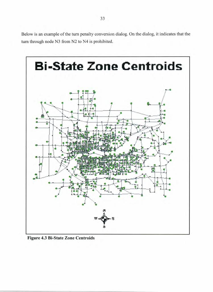
33
Below is an example of the turn penalty conversion dialog. On the dialog, it indicates that the
turn through node N3 from N2 to N4 is prohibited.
Figure 4.3 Bi-State Zone Centroids

34
CQn~rert Turn ~~n~itie~
~~~i~nmenk L~}~er t H i~h~~~~~~ kr~ek~
~en~lk~ T ~~le
Frcm H cue
T~rc~~~ Hc~e
Te Here
~en~lk~
H~
H cn~
~~ncel
Figure 4.4 Convert Turn Penalties dialog box
Once the turn prohibitions were converted and assigned to the correct network,
checks were made to verify that the penalties were indeed effective. The final data file to be
converted was the external matrix. An external matrix is a representation of the trips between
external cordon stations in the model. External cordon stations are similar to zone centroids
and represent the traffic flow into and out of the area being modeled. Data is obtained at
external stations by counting vehicles passing specific points in the transportation network.
Owing to the fact that origin/destination information about external-external trips is not
readily available, growth projections are usually done by using a growth factor applied to
existing cordon counts. These methods are described in some detail on page 10 in the
literature review. Conversion of the TRANPLAN® matrix eetab.98 required renaming the
file to eetab.dat using operating system commands. This was necessary to enable
TransCAD's TRANPLAN matrix import utility to recognize the file as a TRANPLAN®
matrix. Following this, the file was imported using the utility.
FORMATTING THE CONVERTED INPUTS FOR TRANSCAD MODELING
The converted data required formatting before TransCADOO modeling could be
performed. Formatting included the following:
• Combining the separate production and attraction data files into a single PA

file, Redundant colu~uns were removed and missing column headings added.
• The friction factor table required the removal of unnecessary columns and the
addition of column headings for time and trip purposes.
The imported network needed to have a tune column added, the distance
column needed accurate values and the capacity of centroid connectors needed to be
changed front. 0. Zero link capacity would preclude any trips being loaded onto the
network.
THE FOUR STEP TRAVEL DEMAND PROCESS
TransCAD~ allows the performance of the travel demand modeling process via a set
of dialog boxes. The data obtained from the Bi-State Commission included the trip
production/ attraction data and thus eliminated the need to perform trip generation using
TransCADO. It was however necessary to perform trip balancing. Trip balancing refers to
the process whereby trip productions and attractions are adjusted to ensure that the totals are
equal as Produced trips must be attracted somewhere. Trip balancing is necessary because of
the fact that different techniques are utilized in calculation of the trip attractions (usually
regression) and trip productions (usually cross-classification) thus causing differing values
for totals. Shown overleaf is the TransCADO dialog used to perform the balancing technique.
The vectors represent productions and attractions by trip purpose, with the purposes being
defined as follows:
HBW —Home Based Work
HBO- Home Based Other
NHB —Non-Home Based
TRK —Trucks
IEEI —Internal/ External and ExternaUInternal trips
For home based trips, the balancing adjustments were done to trip productions
whereas the other purposes had balancing adjustments done to the trip attractions. It is
generally acknowledged that home based trip production data is more reliable than trip
attraction data. For I~TI-IB, TRK and IEEI trips, the converse is acknowledged to be true.

36
D ata~ie~
~eckor ~ PH ~ PH~O Pf'~H~
1 ~~~P~
Neckar 1 Field
~ ekh4d i
~eckcr ~
R eccrd~ III reccrd~
i~rl ekhcd ~H B H old ~eck1 ~H B H old ~eckl ~f~ H ~ H old ~ect~
PIEEI
Dili '~;'rr~~fpr
~-~ nectar 1 C pkions
J
~`" ~Ilc~► all record values to be cl~an~ed
J
H old values ~eckQr ~ ~eckcr ~
~eckor ~ Field ~AIEEI
J o~ Cancel
C ptions
~ ekkin~s
add a rcp
Figure 4.5 Trip Balance Dialog Box
Skimming the Network (Shortest Paths) Before the trip distribution step was performed, it was necessary to get an impedance
matrix. The updated network file, with centroids and turn prohibitions correctly represented
was skimmed to obtain the desired result. It must be noted that intrazonal travel times had to
be accounted for and the impedance matrix was adjusted accordingly. For the intrazonal
travel times, the TransCAD utility to perform that procedure was utilized. The Shortest Path
and intrazonal travel time dialog boxes are shown below.

37
Line L~}~~r H igl~~~~~~~ kr~~k~
H ~k~~rk ~: gym... ~B i~t~k~~~ ~~~~~~im. n~k
S ~ekking~
~ inimi~~
From 'III F~~kur~s
T ~ III F~~kur~~
~-- ~ kor~ H ~~ulk~
~' F~ ~auk~e ~~sk~rn ~'* ~ akrix File
~an~~l
ttil ~t~~r~
S kim~
~ ~kkin~~
Figure 4.6 Multiple Shortest Path Dialog Box
Intrazonal Impedance Calculation
~ ~trix File ~: ~m~d~Iling~~I~Qrk~~k~ . mkx ~ ~
~ ~trix
F~~t~r ~~lu~~ b~►
a - ~ p~r~kian
~dj~~~nk ~~n~~ 3
~-- T reak ~ i~sin~ ~~lu~~
R ~pl~~~ ` ~~~ _ ~ A~ z~r~ ~ ~~ mi~~in~
~~n~el
~ ~kkin~~
Figure 4.7 Intrazonal travel time dialog box:
Distributing the Trips
Following the creation of the shortest path matrix, the next step involved performing
trip distribution. As mentioned in Chapter 2, the gravity model is the primary technique used
to perform trip distribution. Consequently, the trip distribution pracedure selected was the
gravity model. Inputs included the balanced production attraction data file, the friction factor
file converted from TRANPLAN and the shortest path impedance matrix previously
generated. In some travel demand models, mode split would follow trip distribution but was
excluded from this model however. This decision was arrived at after studying the Bi-State
model execution in TRANPLAN® using the "RUN98" FORTRAN command file. It was

38
ascertained from Bi-State professionals that the share of alternative modes of transport was
not significant enough in the Quad Cities area to warrant inclusion in their model. Hence, the
mode split phase was omitted in the TransCAD model.
Grarrit~ E+raluatian
f~rodra~ki~n-.~kkr~~kion Q ~k~ - --
~ ete~ie~
R ec~r~d~
B elen~e~PA
III Feek~lre~
~ enera~l Fri~ki~on Fe~k~r~
Purpose HBO HBO
oK 1 Oencel
~ ekkin~~
Fri~ki~n Fa~k~r T,~pe ~~~ T e~le T able
t~~~ H E. T at~le TRIO T ~l,la
m- Fri~ckian Faokor I nformekion for ~I H B Feokors Oome from . . .__ _
~" O gimme "` I n~erse
~- Friokion Factor T able _ -~
~ aka~ie~
F Fackor Time
frickion
~ rop ~o~eUp
~I ore ~ own
~` E xponenkiel ~~ T able ~' h~ ekrix
NHB
T1~1E
I~-Fackors I nclu~e I~-Fackcrs
I mpe~ance ~ akrix
~ akrix File
h~l akrix
~ hcrkesk Pakl~ S horkesk Pakl~ - kime
I•'~latr~~. FEIN
I'S~atri<<
Figure 4.8 Gravity Model dialog box
From the above dialog, it can be seen that friction factors are applied by trip type.
This is necessary given the tendency for different trip types to exhibit different trip
distributions. For example, staff at the Bi-State Commission have observed tYiat HBW trips
tend to be longer than trip types such as HBO and NHB trips. IEEI trips with part of the trip
occurring outside the modeled area will tend to be longer.

39
Origin /Destination
In travel demand modeling, trip productions and attractions do not necessarily
represent the actual trip origins and destinations. Home Based Work trips for instance do not
always originate at home but may also originate at the workplace for the return trip home. In
such an example, despite the return trip home originating at the workplace, it is generally
acknowledged that the home was responsible for the production of both the initial and return
trips. Given this situation, it was then necessary to convert the productions and attractions to
actual trip origins and destinations. Shown below is an example of the PA to OD dialog box
available in TransCAD®.
"{"
Convert P-A wlatrix to O-a f~l~trix
I npuk ~--
R ~ ~ akrix File ~ ukpuk ~ atria
R epork H curs ~
Change I nformakicn ~ akrices
TRIG IEEI
To ~24
JJ
R epork each hour separakel~
Use ~akrix FHB
~ Con~rert person krips ko vehicle krips xis
eij~~ F1 ~ t~ ~ ~ ~i 4• Ea •Jt ~r t.~ i ' t ~J ~'~
x _
t~`_~f I;.~ ,~E~1t~ .~~ f i art i
Use vehicle T rips ~-~~ ~~:~ r~~ ~~ Yes Yes
J J
Figure 4.9 PA to OD conversion dialog box
UK
Cancel
The dialog above allows the option of reporting trips hourly or daily. It was decided
after consultation with Bi-State Commission staff to use the daily reporting procedure and
factor the totals to be assigned by a Peak Hour factor. For each trip purpose, a separate OD
matrix was produced thus necessitating a combine procedure to aggregate the data for traffic
assignment. The External-External trip totals also had to be combined with totals from the

40
other trip purposes prior to traffic assignment. To accomplish the tasks described, the
TransCAD~ Matrix Combine and Matrix Quicksum routines were used. Shown below is the
Combine Matrix dialog.
Combine Makrix Files
~~ ~ atria File to ~om~ina ,._.._.,:. ,~..
~alact III
-- ~ pkion
P~to~~ 1 mp~~rkPd T R~,<<J Pl.~~d t~~ akrix
J
~"` I~aap X11 rotes and columns ~` i~aep onl,~ o~rarlappin~ rotes and columns
~~
Figure 4.10 Matrix Combine dialog box
~ancal
Traffic Assignment
After obtaining the OD trip totals, the next phase involved loading the trips on the
network. The network capacity values represent capacities for peak hour travel. This
subsequently required factoring the daily trip totals obtained from previous steps by the peak
hour factors used by the Bi-State Regional Commission. A factor of 10% or 0.1 of total daily
travel was being utilized in the Bi-State model. The assignment technique chosen was the
Equilibrium assignment to ensure consistency with the Equilibrium technique used in the Bi-
State TRANPLAN model. An illustration of the Traffic Assignment dialog is shown.
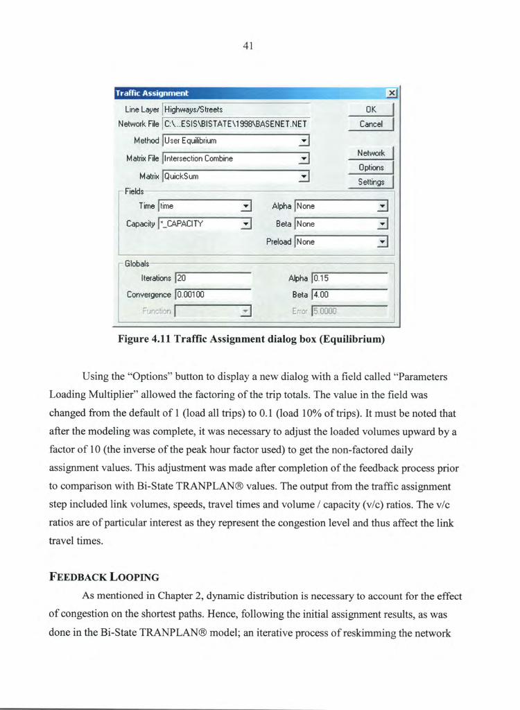
41
Ling Layer ' H i~h~~y~~S kr~~ks ~ ~
t~ ek~rark File C: ~... E ~ I ~ ~~ I ~ TAT E ~1 ~~~~B~~ E H E T .HET Cenael
1~1 ekha~d ~ U per E ~~ilibri~m
~ akrix File I nkerseakian Cambme
~ ekrix I~ uial~~ ~m
Fiel~~ _..~._~~,.,._~
Time
Cepeciky
~kime
'_C~I~~CI T~
~Iphe
~ ete
~relaa~
H ane
Bane
H ane
~! ek~ar~ , ~~ ~ pkian~_, ,~
~ ekting~
J
~-- ~ IQbals I kerakian~
Can~ergenae
~- ~_~t't~1k~ ~t~~
~o.00i o0 ~Iphe
B eke
~.1 b
~a.ao
Figure 4.11 Traffic Assignment dialog box (Equilibrium)
Using the "Options" button to display a new dialog with a field called "Parameters
Loading Multiplier" allowed the factoring of the trip totals. The value in the field was
changed from the default of 1 (load all trips) to 0.1 (load 10% of trips). It must be noted that after the modeling was complete, it was necessary to adjust the loaded volumes upward by a factor of 10 (the inverse of the peak hour factor used) to get the non-factored daily
assignment values. This adjustment was made after completion of the feedback process prior
to comparison with Bi-State TRANPLAN® values. The output from the traffic assignment
step included link volumes, speeds, travel times and volume /capacity (v/c) ratios. The v/c
ratios are of particular interest as they represent the congestion level and thus affect the link travel times.
FEEDBACK LOOPING
As mentioned in Chapter 2, dynamic distribution is necessary to account for the effect
of congestion on the shortest paths. Hence, following the initial assignment results, as was
done in the Bi-State TRANPLAN® model; an iterative process of reskimming the network

42
with updated congested travel times was performed. A rerun of the gravity model trip
distribution process using the newly calculated impedance values accompanied each
iteration. As with the initial steps described above, the ProductionlAttraction to
Origin/Destination step as well as the aggregation with the External/External trip information
was completed. Three iterations were completed and the final assignment results compared
with the Bi-State results. The following steps were followed to perform each feedback
iteration:
1. Set the "Time" variable in the highway/streets file to the maximum travel time
variable "Max_Time" obtained from the joined assignment results.
;r4~_T irn ~_ 7~aa 1.8~Qa ~ _ a$aa 1 _ ~~aa ~ _ 2~aa 1_a$aa ~ _ 2~4aa 2_ a~~1 1.5~~4 4.882 1.2~~a x_571 ~ 1.17Qa 1.2157 2.8714
1~ 'It6_fbw{
~2i
~~~
X50; ~~~ 144: 1 ~8~~,
1493
'15a~ 151:9
_: 1 ~8
Figure 4.12 Illustration of "Time" Column with "Max_Time" Column values
~. ~8aa ~ . aaaa 1. Qsaa 1.~2aa 1.24ao 1. Q80Q 1.2~aa ~. a945 1.~42~ ~. ~as~ 1.28aa 0.51 ~ 1.~ Sao 1. ~13~ 2_~~'1 ~
~_ ~ saa 1 _saoa 1 _a80a ~ _32oa 1.240a 1 _a80a 1.240a 2_a9~5 1.542 4.80~~ 1.280a x_571 ~ 1.17Qa 1.215 2.871 ~
3.~8 1.80 1.a8 1.32 1.24 1.a8 1.24 1.44 1.54 4.55 1.28 x.57 1.17 1.15 2.87
23.7815 23.3187
5.5aaa 74.15aa 1.5aaa
185.6aaa 892.95aa 792.894a
1 x98.1818 317.35aa
0_aaaa 1178.518a
4x.8797 435.828a 139. x838
2. After the "Time" variable was updated in the Highway/Streets table, it was then
necessary to update the network file with the new travel time and perform the shortest
path network as illustrated above. The following is an illustration of the TransCAD®
dialog for updating network parameters.

43
Update h~etwark
I~ pr~~k~
E n~al~~D i~~~l~ Linl~~ ~ pki~n
~~ of i~
~ ~ ~h~n~e
Linl~ C~~k~ I~ p~at~ c~~k~ ~n III links
~ ~k~r~rk Fi~l~ I n Ling L~~~r L~ngkh x ~P~CIT~ h~i i~
~ pd~k~ n~~~ ~c~~k~ ~`'~ tV;' ~ fit`=,~ ~f ~ fti`, ~`'~ s'~ t,..~!~' ~ ~ t?_~ F
~~~ ~~~
J
Figure 4.13 Network Update dialog
3. The trip distribution, PA to OD, matrix aggregation and traffic assignment steps
described earlier were repeated three times and the resulting TransCAD® assignment
map is shown below with screenlines.

44
Feedback Volumes with Screenlines
~~ ,~"`: _
s ~ ~f~~ ::
... .. . ~i ~
Figure 4.14 Screenlines
COMPARING 1998 ASSIGNED RESULTS
Using the TransCAD~ screenline tool it was possible to obtain the flows across
selected important links and have them compared with the Bi-State model results. The Bi-
State values were represented in an ESRI Arcview~ DBASE IV file containing a traffic
volume assignment attribute. The Bi-State values and the TransCAD~ values were then put
in a common DBASE file and compared.
To perform the comparison, several tests were applied including Root Mean Square
Variance analysis on the difference in the compared results, percentage difference on key
cross river and freeway links and the percentage difference between the TransCAD~
assignment totals and the Bi-State totals. As mentioned in the Model Validation and

45
Reasonableness manual, (16) these tests are standard validation checks used in travel
modeling. The following table shows percentage differences on key links in the Bi-State
model. Consultation with Bi-State modeling professionals indicated that focus should be
placed on the links selected. These links represent the Mississippi River crossings and the
interstates near the cordon points in the map.
Table 4.1 1998 Assignment Differences on Key Link
4525 4526 776 5so6 752 5602 761 846
4101 5614 1242 5618 5132 5622 4534 4787 3318 3347 3317 3320
15250 15250 10800 10800 7600 7600 9150 9150 8850 8850
36100 36100 11$00 11800 13300 13300
7100 7100 8400 8400
14536 14536 9022 9162 7154 6929 8643 8816 7895 8290 32474 32024 12161 12264 12902 14215 6652 6690 7770 7873
so~ulf ':eren~_
714 714 1778 1638 446 671 507 334 955 560 3626 4076
361 464 398 915 448 410 630 527
5 5 1s 15 6 9 6 4 11 6 10 11 3 4 3 7 6 6 8 6
Upon observation of the table, it can be seen that the maximum percentage difference
was 16aIo with the majority being below 10%. It was thus decided that such variances were
acceptable after consultation with the Model Validation and Reasonableness manual. { 16)
To verify this conclusion, the other tests mentioned such as the comparison of all
links and RMSD were performed. when all links were compared, the total for the Bi-State
model was 10,737,298 trips while that for the TransCAD® model was 9,326,533 trips. This
gave an absolute difference of 1,410,765 and a percentage difference of approximately 0.13
or 13%.The file of all the links is not referenced owing to size. Performance of Root Mean
Square analysis on the links crossed by screenlines shown in Figure 3.0 indicated a °IoRMSD {Root Mean Square Difference) of approximately 26°Io. {See Appendix E} The percentage
RMSD was calculated using the following formula.
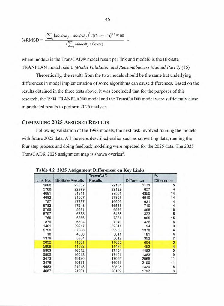
46
( . (Modela ~ - Modelb ~ )2 /(Count -1))0'5 * 100 J J %RMSD = J
(~ .Modelb /Count) l
where modela is the TransCAD® model result per link and modelb is the Bi-State
TRANPLAN model result. (Model Validation and Reasonableness Manual Fart 7) (16)
Theoretically, the results from the two models should be the same but underlying
differences in model implementation of some algorithms can cause differences. Based on the
results obtained in the three tests above, it was concluded that for the purposE;s of this
research, the 1998 TRANPLAN® model and the TransCAD® model were sufficiently close
in predicted results to perform 2025 analysis.
COMPARING 2025 ASSIGNED RESULTS
Following validation of the 1998 models, the next task involved running the models
with future 2025 data. All the steps described earlier such as converting data, running the
four step process and doing feedback modeling were repeated for the 2025 data. The 2025
TransCAD® 2025 assignment map is shown overleaf.
Table 4.2 2025 Assignment Differences on Key Links
Link No. Bi-State Results TransCAD Results Difference Differen~~e
2680 23357 22184 1173 5 5788 22979 22122 857 4 4681 31911 27561 4350 14 4682 31907 27397 4510 14 757 17237 16606 631 4 5782 17248 16538 710 4 5795 5631 6526 895 16 5797 6758 6435 323 5 766 6366 7331 965 15 879 6804 7240 436 6
1401 39217 39311 94 0 5798 37886 39256 1370 4 18 4830 5011 181 4
1378 5364 5012 352 7 2032 11001 11605 6C14 5 5808 11032 11485 4~>3 4 5803 16012 17494 1482 9 5805 16018 17401 1383 9 3473 19130 17065 2065 11 3476 19131 16941 2190 11 4683 21918 20598 1320 6 4687 21901 20109 1792 8

47
2 25 TransGAa Model Results
~_~~~ ~ -__
i
a _~
3
~~r
9 --~ s __ -- ~ _
:%
4
3- ~~~~=-
~ ~ - _ a ~- _ _ _ __ a
-~ ~_
5~
' ~ _ ~_~` ~i_<, -nom _ 3-= -
_~ a ~~ _ = ~~—~
~ 6.~
~'y--a~_32~z ~ _ O 1~}"i~is ~3 ~ ~ Via:. E_. 3 3._ ~--. ~.a..~~ -~ i '~ ~ ~-
~~~ ~~_ S
~~=
0a ~
~4
~—
~23
_ ~ ~
roT Fio~v ~_ 7~~i~ ~7~~~ ~1~ 7~~
Figure 4.15 2025 TransCAD Research Assignment Results

48
Like the 1998 results, no difference was greater than approximately lfi% with the
majority of the links reporting differences below 10%. It may be noted that the links
highlighted represent an additional Mississippi River bridge crossing representing a planned
network improvement. The percentage Root Mean Square difference calculated for all the
links was determined to be 28%. The %RMSD calculated on the links crossed by
TransCADC~ screenlines (links with significant traffic volumes) illustrated in the map above
was determined to be approximately 13%. See Appendix E. The percentage difference
between the trips assigned on all links in the Bi-State model and the TransCAD~ model was
4%.
Given all this information, it could be concluded that for the purposes of sensitivity
analysis, the model predictions were close enough to warrant proceeding to the sensitivity
testing phase of the research. In sensitivity analysis, it is not critical that the models match
exactly since the main objective is to analyze changes in model output. In .travel and
emissions forecasting however, it is important that the absolute output values are as accurate
as possible given that large expenditures of money, time and effort may be dependent on the
forecasted values.

~7
CHAPTER 5. PERFORMING SENSITIVITY RUNS ON TRANSCAD MODEL
SENSITIVITY ANALYSIS
Sensitivity analysis is defined as "the process used to ascertain how a given model
output depends upon the input parameters. This is an important method for checking the
quality of a given model, as well as a powerful tool for checking the robustness and
reliability of its analysis. The topic is acknowledged as essential for good modeling practice,
and is an implicit part of any modeling field".
In this research, the aim is to determine which input factor affects the output emission
results by the greatest magnitude. Using the basic principles of sensitivity analysis, the model
inputs were adjusted and the output from each run noted, After completion of all model runs,
the difference in output emissions levels could then be statistically compared using any of a
multitude of techniques. Some useful techniques include regression analysis and ANOVA
(Analysis of Variance).
Sensitivity analysis can be applied in a variety of modeling situations. For example, it
can be applied to econometric models where future economic attributes such as GDP (Gross
Domestic Product) are predicted. Another relevant application is the study of the effect of
transportation investments on land use changes. Sensitivity tests in econometric modeling
would, for example, enable economists to determine how varying assumptions about interest
rates, energy prices, labor costs would affect the actual GDP results.
Sensitivity tests can also be applied to physical models such as hardware control
systems. In such applications, the objective is to study the response of the system to varying
input conditions such as electrical current, feedback noise {incoherent and corrupted control
signaling) and load affect for example motor speed, response time to changes in inputs etc.
{22)
A common use of sensitivity tests is the estimation of parameters that represent
continuous variables in experiments where it is impossible to measure the values in actual
practice. (22) For example sensitivity testing of pyrotechnics to ignition will allow a
relationship to be obtained between the stress levels and ignition below the critical threshold
pressure, above which samples always ignite. Without sensitivity testing, it would not have

50
been possible to obtain estimates of the parameter since application of pressure to
pyrotechnic samples inevitably destroys or damages the sample and makes it impossible to
do repeated testing on a particular sample. This technique is known as Maximum Likelihood
Estimates and is being increasingly applied to sensitivity analysis. Other common techniques
include Probit, Bruceton, Robbins-Monro and Langlie. {22)
The mathematics involved in such tests can become complicated and it is considered
beyond the scope of this thesis to analyze the various techniques. In concluding, it can be
said that sensitivity analysis allows the following to be achieved:
1. The effects of accuracy in a modeled system can be determined.
Z. 'The effects of changes in both magnitude and direction in a modeled system
can be determined.
3. Facilitates model calibration.
SENSITIVITY TESTING PROCEDURE As stated in the introductory section on research questions, the main goal of this
research was to determine which of three input factors has the greatest effect on the predicted
emissions output. The input factors considered in the research include
1. The traffic assignment methodology used. Five assignment techniques were
investigated including stochastic, user equilibrium, stochastic user equilibrium,
incremental and capacity restraint.
2. The use or non-use of dynamic feedback modeling.
3. The type of the friction factor distribution used. (3 distributions were used)
Determination of the most significant factors on the emissions output required
running the model over all combinations of levels of the input variables. Each combination of
levels represented a unique sensitivity scenario resulting in different output values. In total,
30 combinations of inputs were used giving 30 emissions outputs. (5 Assignment levels x 2
dynamic modeling levels x 3 friction distributions.)
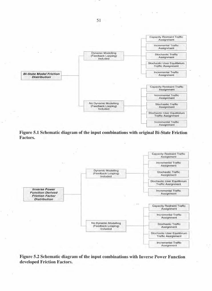
51
Capacity Restraint :Traffic Assignment
Incremental Traffic Assignment '.
Bi-State Mode/ Friction Distribution
Dynamic Modelling (Feedback Looping)
Included
No Dynamic Modelling (Feedback Looping)
Included
Stochastic Traffic Assignment
Stochastic User Equilibrium Traffic Assignment
Incremental Traffic Assignment
Capacity Restraint Traffic Assignment
Incremental Traffic ,Assignment
Stochastic Traffic Assignment
Stochastic User Equilibrium Traffic Assignment
Incremental. Traffic Assignment`
Figure 5.1 Schematic diagram of the input combinations with original Bi-State Friction Factors.
Inverse Power Function Derived
Friction Factor Distribution
Dynamic Modelling (Feedback Looping)
Included
No Dynamic Modelling (Feedback Looping)
Included
Capacity Restraint Traffic Assignment
Incremental Traffic Assignment
Stochastic Traffic Assignment
Stochastic User Equilibrium Traffic Assignment
Incremental Traffic. Assignment
Capacity Restraint Traffic Assignment
Incremental Traffic Assignment
Stochastic Traffic Assignment
Stochastic User Equilibrium Traffic Assignment
Incremental Traffic Assignment
Figure 5.2 Schematic diagram of the input combinations with Inverse Power Function developed Friction Factors.

52
Capacity Restraint Traffic ;4ssignment
Incremental Traffic .Assignment
/n verse Power Function Derived
Friction Factor Distribution
Dynamic Modelling {Feedback Looping)
Included
Stochastic. Traffic Assignmen#
Stochastic User Equilibrium - Traffic Assignment
Incremental Traffic Assignment
Capacity Restraint Traffic. Assignment
Incremental Traffic Assignment
No Dynamic Modelling Stochastic Traffic (Feedback t_ooping) Assignment
Included Stochastic User Equilibrium'
Traffic Assignment
IncrementalTraffic Assignment
Figure 5.3 Schematic diagram of the input combinations with Inverse Power Function developed Friction Factors.
For each combination of inputs, the procedure followed involved performing the
sequence of steps described in Chapter 4 including trip distribution, PA to OD, trip purpose
combination and traffic assignment. The sequence of steps described in Chapter 4 for
feedback modeling was performed for corresponding feedback input factors. In non-feedback
modeling, the travel modeling process was halted after the first assignment results were
obtained using the initial skim network.
FRICTION FACTOR DISTRIBUTIONS
Friction Distribution 1 The first set of friction factors used in the model was simply the friction factor file
supplied from the Bi-State Commission and converted for TransCAD®. In addition to using
tables developed from observation of actual conditions, it is also possible to develop friction
factors by using impedance functions. In general, friction factors are inversely related to

5~
impedance (travel time, distance, cost etc.). As a result, a simple inverse function can be used
to develop friction factors. Such a function would take the form f(d;~) = d;~-1 where:
• d;~ =impedance between zones i and j
• f(d;~) =friction factor between zones i and j
It has however been shown that the simple inverse function is not the best performing
impedance function (11). Hence, more complicated functions have been devised that have
been shown to perform better. Among the more popular functions are the exponential
function, the inverse power function and the gamma function. (11) —c(d;~ )
exponential .f ~dij~ — e where c is constant > 0
-b inverse power .f ~d ~~) = d i~ where b is constant > 0
-b - ~(di~ gamma f (d ~~) = a • d l~ • e where a > 0 and c >= 0
Source: Travel Demand Modeling with TransCAD 4.0 page 176.
It should be noted that the ganu~na function is a _combination of the inverse power
function and the exponential function. Application of these functions involves adjusting the
parameters a, b or c to replicate the actual conditions found in the modeled area.
Friction Distribution 2
The inverse power function was applied and a new friction factor table developed for
friction distribution number 2. The parameter chosen for b was 1.45. Application of this
function and parameter gave a distribution that had a sharper curve {more L shaped) than that
of the original B i-State data. The factors calculated for long trips were higher. Theoretically,
such a difference should result in proportionately fewer intermediate distance trips but more
very long and very short trips.
Friction Distribution 3
In this case, the gamma function was applied. The values chosen for a, b and c were
1, 1.45 and 0.025 respectively giving a very sharp distribution curve. In addition the row
corresponding to a time of 1 minute was removed with the gamma being applied from time 3
minutes onwards. The maximum friction factor value of 10,000 was used for all times t = 2

54
minutes or less. The overall result of this application was the most L like distribution of the
three being evaluated. Theoretically, based on this distribution, there should be a larger
number of very short trips than was the case for the previous two. In addition, the friction
factors at higher travel times were lower which should lead to fewer long trips in the model.
Bi-State Friction Factor Distribution
6000
5000
4000
0 3000
•" 2000 LL
1000
~ .___- i ~ i_ ~_ T
__ ~
__ i
_ ~ i i I ~ L
1 3 5 7 9 11 13 15 17 19 21 23
Time (minutes)
Figure 5.4 Bi-State Friction Distribution
Please see Appendix A for corresponding friction factor tables.
HB W
HB 0
N I-~
TRK
IEEI

55
Inverse Power Function Friction factor Distribution
6000
5000
4000 m
0 saoo .~ Z000 LL
1000
~ ---1- -~---- T---- 1-----~- ---T
7 9 11 13 15 17 19 21 23 25
Time (minutes)
Figure 5.5 Inverse Power Function Friction Factors
HB W HB 0 N HB TRK
IEEI
EFFECT OF VOLUME ON TRAVEL TIMES (IMPACT OF FEEDBACK MODELING
With the exception of the All or Nothing and Stochastic assignment techniques, all
traffic assignment methodologies incorporate a volume delay relationship. This better
describes the actual impact of traffic congestion on network travel times. The most common
function used to describe volume delay is the Bureau of Public Roads relationship. This
relationship is defined as (17)
t=t o l+a ~v R
~c
where: t =Congested link travel time
tO =free flow travel time on link
v =link volume
c = i capacity

56
a, ~3 =calibration parameters.
Source: Travel Demand Modeling with TransCAD 4.0 page 176.
Gamma Function Friction factors
6000
5000
,~° 4000
~ 3000 0
2000
1000
o , 1 3 5 7 9 11 13 15 17 19 21 23
Time (minutes)
I~ w HB 0 N HB TRK IEEI
Figure 5.6 Gamma Function Friction Factors
Historically common values used for a and ~i are 0.15 and 4.0 respectively. Based on
such values, it is easily recognized that as soon as the v/c ratio tends to 1 and above, t
becomes much larger than to.It must be noted that v/c ratios greater than 1 are possible only
in theory given that a roadway cannot possibly accommodate a greater volume than its
capacity dictates. Such a situation could thus be interpreted as unmet trip demand along a
particular link. Other volume delay functions have been utilized but is generally recognized that by simply adjusting the parameters a and (3, most of the other functions can be
approximated by the BPR function.

s~
As described in Chapter 2, this volume delay effect can significantly affect validity of
the assigned results. Initially, uncongested travel tunes are used to obtain the trip assignments
but in reality, the congested times must be utilized to give realistic assigned results. Hence
the use of feedback loops where the congested travel times are fed back to the network
skimming (shortest path) phase. This in turn affects the trip distribution and finally the
assignment results. Runs were performed both withlwithout feedback for all three friction
factor distributions.
TRAFFIC .ASSIGNMENT METHODOLOGIES
For each combination of friction factor distribution and feedback/no-feedback, the
five traffic assignment techniques mentioned at the beginning of this chapter were utilized.
This was accomplished by varying the option selected in the TransCAD® Traffic
Assignment dialog box. Shown next are the dialogs for each of the other four techniques used
in addition to the I~ser Equilibrium illustrated on page 41.Of note are the disabled capacity,
alpha and beta fields in the Stochastic Assignment dialog box. That is expected given the fact
that the Stochastic assignment technique does not rely on the volume delay BPR function and
its associated parameters illustrated earlier. Following the completion of the 30 sensitivity
combinations of inputs, it was necessary to produce and analyze the emissions results.

58
Traffic A~~ignment
Line Layer H i~h~a~~~'S kreek~
I~ek~orl~ File ` ~:~f~1~D~ELLIf~I~~BI~If~11~lET. JET
~ ekho~
~ akrix File
~ akrix
Fiel~~ ._._,._,.. i _ _
Time ~ kime i
~apaoity
~ lobal~
I kerakior~~
~or~~er~er~oe
~a~a~~ik~,~ ~~ e~:krair~k
I t~ker~eotion ~ombir~e
~ ~iol~B um
~. 01 ~~
Figure 5.7 Capacity Restraint
Lina Layer H i~h~ay~~B kreek~
~l ek~orl~ File ~: ~~1 ~ ~ E LLI ~I ~ ~B ICI ICI ~I E T . ICI E T
~ ekho~
~,Ipha
~ eta
Preload
~ akrix File
~ akrix
~ Fiel~~ .._.~_
Time
Capacity
riorer~ier-~k.~l
r~ker~eokion combine
~ ~i~cl~B Wm
kima
C~P~CI T~
~ lobal~ (terakior~~
Cor~~er~er~ce
F~;r-~t:~~ic~r-~
~Ipha
B eka
Preload
~lorie
~ f~ ore
Hone
~0~7
~~
~ar~oel
N ek~orl~
~ pkion~
~ ekkin~s
_I
~~
~ar~~el
t~ et~ork
0 pkion~ ~_~- , Sekking~
Hone T
~) one
H ore
~zo ~o.a100
Figure 5.8 Incremental Assignment
~Ipha
Beta
s:. f~~~s
0.15
a.oa

59
Line Le~!er H i~h~e~~~~ kreeks
I~ek~~rl~ File ~:~~1~DDELLII~~~~I~II~I~IET.~IET
f~ ekh~ad
I~rl ekrix File
h}I ekrix
~- Fiel~~ f
{ Time
~epe~ik~
:, r~~~:h.3 sti~~.~1._.~~..~
~a~.~ili~ri~.ar~i
nkerse~tion E~mbine
kime
G labal~
~Iphe
B eke
~rel~e~
f~l one
~J one
I~ one
~~
~~ncel
H ek~~rl~
~ pki~n~
~ ekkin~~
(kereki~n~
~~n~er~en~e
F~n~ki~n
~20
~. ~1 ~~
H ~rm~a) J
~Ipl~e ~.1 ~
~ eke
E rr~r ~. ~~~~
Figure 5.9 Stochastic User Equilibrium
Line Leer H i~h~e,~s~~ kreek~
f~ ek~~rl~ File
~ ekh~d
~ ekrix File
~ ekrix
r~ Fields
~:'~~1~[~ELLIt~~~~I~If~II~ET.f~ET
nker~ecki~n C~m~ine
~ ~i~l~~ ~m
kime
J
F=_~r;i~.kiE,r~
Figure 5.10 Stochastic Assignment
F ! ~,(prtn
E ~~:.
E rr~r
OK
~en~el
H ek~r~rk
~ pki~n~
~ ekkin~s
60
CHAPTER 6. LINKING TRAVEL MODEL OUTPUT WITH EMISSIONS RESULTS
MOBILE 6 EMISSIONS FACTOR MODEL
Following the completion of the sensitivity runs in the TransCAD~ travel demand
model, it was then necessary to obtain emissions factors and combine the results as described
in the introductory chapter on page 2. The tool used to get the emissions factor results for this
research was the Environmental Protection Agency's (EPA) MOBILE6. The MOBILE6
program is supplied with a number of tables that represent the defaults values to be used in
the absence of specific information for the area under study. These tables were developed
from data collected in the FTP tests and from numerous jurisdictions across the country.
Among the tables included are the vehicle age distribution, mileage accumulation rates, VMT
fractions, average speed distributions and many others used to ultimately calculate the
average emissions rate per vehicle.
MOBILE6 calculates emissions for three of the criteria pollutants including oxides of
nitrogen (NOx), carbon monoxide (CO) and volatile organic compounds (VOCs). Ozone
(03), another criteria pollutant, cannot be directly calculated with the MOBILE6 program
given the fact that ozone is a secondary pollutant. Low level ozone is formed by complex t
atmospheric reactions in the presence of sunlight (energy source) between atmospheric
oxygen 0 2, nitrogen oxides (NOX) and hydrocarbons (HC). (23)
MOBILE6 is a command line based FORTRAN language program requiring an input
command file that directs the program to generate the desired options and output formats.
Two input files were used for this research; one representing emissions data for arterial
streets and the other representing emissions data for freeways.
Roadways are classified by MOBILE6 into 4 types: (24)
1. Freeway :- High speed, limited access roadways
2. Arterial :- Arterial and Collector roadways
3. Local :-Urban Local Roadways
4. Fwy Ramp :-Freeway on and off ramps.

61
For the purposes of this research, only the freeway and arterial categories were
analyzed given that insufficient travel network detail was available to properly include local
roadways and freeway ramps.
The input files to MOB ILE6 allow several default parameters to be specified so that
the model can be tailored to local conditions. For this research, the primary items adjusted
were the speeds, season, temperature and oxygenated fuels components. For 2002 in Iowa, a
significant proportion =~ 55% of the gasoline sold in the state was a 10% ethanol 90%
gasoline blend regarded as an oxygenated fuel. (2~~ At this blend, the oxygen content in the
fuel is about 3.5% resulting in > 30% reduction in ~O emissions particularly in winter. (2b)
As a result, it was decided to utilize the MOB ILE6 oxygenated fuels command to more
accurately represent the actual situation in Iowa. Illinois, the other state in the B i-State area
also has a significant percentage of ethanol-blended gasoline sales. Illustrated below is an
example of a portion of the input file for freeways with the selected options .
MOBILE6 INPUT FILE : DATABASE OUTPUT ; AGGREGATED OUTPUT WITH FIELDNAMES
DATABASE EMISSIONS :2222 2222 DATABASE FACILITIES: Freeway DATABASE VEHICLES :22222 22222222 2 222 22222222 222
RUN DATA MIN/MAX TEMP : 70. 90. SEASON : 1 FUEL RVP : 7.0 OXYGENATED FUELS : 0 .55 0 .035 2
SCENARIO REC :Scenario Title Text -Freeway 2.5 CALENDAR YEAR :2025 AVERAGE SPEED : 2.5 Freeway EVALUATION MONTH : 7
Figure 6.1 Freeway MOBILEf Input File

6~
The MOB ILE6 -input file is divided into three sections; the Meader section, the Run
section and the Scenario section. Shown above are the header section, one run section and
one scenario section. The full input files far both freeway and arterial are shown in Appendix
B.
Header Section
The Header section controls the overall input, output and execution of the program.
(4) Options specified in this section apply to all runs and scenarios defined in the file. in the
example shown, the DATABASE OUTPUT option was chosen to allow output in a database
file format that would facilitate processing in Visual Basic. In addition, it was also specified
to aggregate the database output over daily time periods given that the TransCADC~ link
volumes were also for daily time periods. The DATABASE EMISSIONS and DATABASE
VEHICLES connnands were used to specify that all emissions. and vehicle categories be
reported in the database output file. The DATABASE FACILITIES cor~~mand was used to
specify the kind of roadway being analyzed. In the above example, freeways and other high
speed divided roadways were being analyzed.
Run Section
The Run section identified by the RUN DATA command is used to define specific
options that apply to local or customized situations. In the above example, each run
corresponded to either the winter season or the summer season. The MINlMAX temperature
command was used to specify the minimum and maximum ambient temperatures that in the
illustrated case above were set at ~0° F and 90° F respectively. The SEASON command of 1
specified summer conditions whereas the fuel RVP specified the fuel Reid Vapor Pressure in
PSI (Pounds per square inchj. The OXYGENATED FUELS command was used to specify
that 55% of the gasoline fuel sold contained ethanol and the oxygen content was 3.5% of
total fuel mass based on a 1:9 ratio of ethanol to gasoline. For diesel fuel applicable primarily
to heavy trucks, the MOBILES default diesel fractions were assumed.

63
Scenario Section
This section details the individual circumstances for which emissions factors were to
be calculated. In the example above, each scenario corresponds to a different average speed
value starting from the low speed of 2.5 mph up to 65 mph. For each scenario, the
CALENDAR YEAR input was set to 2025, the year being modeled. The AVERAGE SPEED
command was used to set the average speed for each scenario along with the roadway type.
The EVALUATION MONTH determines whether calculations should be done for January
or July. In the example given, the month was set to July corresponding to summer.
Shown below is an example of the MOBILE6 command line DOS input illustrating the use
of the "Freeway" input file.
C:'~tiMODEII~~ 1 ~,MaBILE6'~Pragram'~Run~,I~ILC-fr.El~ -~,_
~ ~ —hit Pa t~~~ t• f a ~• La}~~ ~ ~a input ~ t• ~ ~~ t ~ m~ P}~a~• Lap' ~ 38~ ~ 1~~~—Ext~ndct•Ctm~ I~et•~ ian 8 _ ~~
~a py~• i~}~t ~ ~ ~ 1 ~ S 6 —~ 6 Phat• Lap ~ a f t ~~~~re r Inc _ Available M~mat•~ = 1~~5~ }{l~
OB I LE6 ~ 16 —Jan —~ 00~ ~
ntct• t}~e name of t}~e Mabilef~ input file: ~•e a ~~1a~
I n put f i lc name : FREE~~~A ~. I N
Pt•ace~~iny ~tat•t times i~ 1 :56:1M.3?M_
Re pa t•t ~ i lc : FREE~~~A ~ . T X T ' e ad in y in f a •mat is n . 'e~•fa~•min~ calculatian~. ' re pat• in ~ a ut put . 'et•~arminy calculat ian~ . i
Figure 6.2 MOBILE6 Command Line Interface
Following the MOBILE6 runs for the freeway and arterial cases, two database files and two report files were produced. The database files were subsequently used in a Visual Basics VB program along with the TransCAD~ link volume files to produce emissions per link. The report files were used to manually validate some of the results calculated obtained by the VB program in a random manner. Shown below is a portion of the report file illustrating the output from one scenario. (Speed = 2.5 mph)

b4
* MOBn~E6 { 16-Jan-2002) * input file: ARTERiAL.iN (file 1, run 1).
* Scenario Title Text -Arterial 2.5 * File 1, Run 1, Scenario 1.
* A user supplied arterial average speed of 2.5 will * be used for all hours of the day. 100°0 of VMT has been * assigned to the arteriallcollector roadway type for all * hours of the day and ail vehicle types.
M 48 Warning: there are no sales for vehicle class HDGVBb
M 48 Warning: there are no sales for vehicle class LDDT 12
Calendar Year: 2025 Month: July
Altitude: Lo w Minimum Temperature: 70.0 {F)
Maximum Temperature: 90.0 (F) Absolute Humidity: 75. grainsllb Nominal Fuel RVP: 7.0 ps i
Weathered RVP: 7.4 psi Fuel Sulfur Content: 30. ppm
Exhaust UM Program: ~To Evap UM Program: No
ATP Program: No Reformulated Gas: No
Ether Blend Market Share: 0.000 Alcohol Blend Market Share: 0.550 Ether Blend Oxygen Content: 0.000 Alcohol Blend Oxygen Content: 0.035
Alcohol Blend RVP Waiver: Yes Vehicle Type: LDGV LDGT 12 LDGT34 LDGT HDGV LDDV LDDT HDDV
MC All Veh GVWR: <6000 >6000 (All)
VMT Distribution: 0.2788 0.4388 0.1507 0.0365 0.0003 0.0022 0.0876 0.0051 1.0000
Composite Emission Factors (glmi): Composite VOC : 2.536 2,513 3.643 2.802 2.997 0.122 0.361 0.772 8.57 2.581 Composite CO 18.79 20.43 25.50 21.72 30,76 2.126 1.637 1.417 103.8b 19.830 Composite NOX : 0.534 0.625 1.020 0.726 0.253 0.051 0.293 1.531 1.03 0.726
Figure 6.3 MOBILE b Report File

65
As indicated earlier, a custom designed Visual Basic® program was used to
automatically calculate the total emissions per network link. The program was used to check
link speed, get emission factors for that speed, get the link VMT and calculate the product of
the two. (Link emissions =emission factor *link volume X link distance in miles) A
flowchart of the process is illustrated.
Network Link assignment volume.:.:.files..
F database fle emissions fro
IV60BILE6
T
load link volume file
r"/~eppend Emissions attribute to link
volume file
ed files (tenter, Summer) CO enter, Summer) NOX (tenter, Summer) VOCs
Get weighted CO `pollutant emissions for
aIM vehicle types for summer .. . , E x ;
pollutant emissions fo all vehicle types for
Get weigh ed l pollutant emissions fo: ' all vehicle types for
~.,..x =~~sur~r~er
pollutant emissions ~~ all vehicle types for
winter .
_T Get weighted NO
;,pollutant emissions fo 3' all vehicle types for
pollutant emissions all vehicle types for
~~~ summa
1 ':.pollutant emissions fci
all vehicle types for
Y ~ Get weighted VOC
pollutant emissions for all vehicle types for
summer
Get weighted CO pollutant emissions for
ail vehicle types far winter
Get weighted NOx pollutant emissions for
all vehicle types for winter
T Get weighted V'OC
pollutant emissions for all vehicle types for
winter
,~
Figure 6.4 Overall Procedure to Obtain Link Emission Results
database f le emissions from '.
~1lIC?BlLE6

66
Process Summer. Emissions from MOBIL
freeway and arterial database files
- ~
Process Winter _. Emissions from MOBILE6
freeway and arterial _ database files
Figure 6.4 Cont' d
The following is a flowchart of the subroutines described above to process winter and
summer emissions from MOBILE6 database files.
freeways
;Get Appropriate emission rate value from freeway
emissions database " (NOX, VOC and CO)
.Begin
T
Link Volume Records
More Records?
Yes
Check Link Speed
Check link facility type (freeway, arterial and
collector}
T
No
:Link emission = emmision ::rate *link distance *link
volume (link VMT)
T Update VOC, CO and NOX link emissions
-data files
arterial roadways
Get Appropriate emission rate value from arterial
emissions database NOX, VOC and CO)
Figure 6.5 Winter and summer processing subroutine

~~
the visual BasicO code is illustrated in Appendix C. ~'he subsequent emissions
results were then aggregated for all the network links in the model. Results are presented in
Chapter 7. SPSS ANOVA analysis of all links along with the aggregated emissions table
mentioned above was then utilized to arrive at conclusions on the input model factors having
the greatest effect on overall emissions output. Also discussed were the differences in
emissions outputs per pollutant for winter and summer conditions.

68
CHAPTER 7. RESULTS
The tabular results of the sensitivity analysis process are presented in this chapter.
The first table presented describes the overall emissions results for all links and both the
winter and summer seasons. Following this, the tabular results for some of the selected links
including approximate speeds and the VMTs are presented. The remaining results not shown
here are described in Appendix F. Finally, a summary of the averaged emissions results over
these 20 selected links is presented.
The 20 selected links consisted of a mixture of high speed, high volume links and low
speed, low volume links. Analysis of these individual links helps to illustrate trends that are
masked with aggregated results. An example of such an occurrence would be one link
registering large changes whereas another similar link showing little or no change. Figure 7.1
below illustrates the selected links.
S~le~c~~~cl Link
~' • :.., ~. _ ~~'~ awe ~~~
:: ~~
~~ 4~ # t_ »
t • ~T r~
i +'~!~ .f
1~,~1~~ L~~r ~ t! ~~+et~ ~'h t~ rr~~tl ~r~ ~.
Hi ~~ ~~~~tr~~ -t~ ~~ I ~~ti ~rti ~~~ ~ ~~I~~c-ti~rti
Figure 7.1 The 20 Selected Links

69
Table 7.1 Total Emissions Results by Input Facto, Season, anti Pollutant --f-z ~-,~~ -~~~^_ - ~~~=
_ -~ -
--~~~~~ ^~ ~ ~
- ~_.~=~ +~
~ - _ _
~^____~~~_. ,.
- - =~_~~=T ~' ~ ~ -s - -= ~~=~ ~ ~~
~_ _ ~~ _~~ ~"s rte`-~~-~_"" ~~'
_-- -_ ~~- r ~_~ f' -~-'-. ____' S _' _=---nom_-~_=~ ~' '~ x~--_ rr„si -
~
-_~ __ -- _- cf"= _ s 3~"~y`<<R r
~ ~~-' -c~n~ -._
._=¢_~ r~" __ ~_~-x=~- ~~-:' `.
z z_ss2~'c~-u- ""cam_ :_ _ ~.~a ~' - =._e=e-~c-'"r__a
~ `~ ~a aselsri4- ,~~s--tv
_ ~ ~_ ~ 3~_
~ 3 - _. _ _ _ - _ _ _~_ _ . ~~ ~6 _ $
.~- ~ ~~~ 'e~l. ^y~ t°E ~~~'i~
~ '~~-.._ ~
- - ~~ ~ ~
_- ~_ ~q
~~~~ S'e _
_. ~."gc f1 ~. _ _ - ~ ' ~ T .
S£~=_ ..- _- _ }y
~ -
~ - y' ~ ___
~
_ __ _ __
~ ~
___ ___ _-
_ s ~_~
~
F T --4.~ _ ..IFS a iP3-~~
6 '~
~ 'Y +t3 =-~
}~ ~ ~y
- -S
~ ~- _ - - - ~ _ _ ~ - _" ~ .~~ ~ ~1 ~
Capacity
~ $ uS _ - r_a ~ s~ -C'_= mac- __ = y _ c~c.~ - z ___ _ _ c y.~'~--! _ _ 4 _ _ _ ~ G ~- . _ aoE _ _ -_ _.__ ~ ---?
1 1 S` Yes Restraint 147,825,931 4,159,144 3,643,655 55,948,335 3,381,116 2,976,097
2 No 118,397,237 3,346,661 2,854,652 45,076,925 2,719,986 2,320,827 User
3 Yes Equilibrium 147,875,213 4,158,125 3,663,714 55,935,360 3,38 i ,509 2,997,879
4 No 118,367,036 3,344, i 55 2,856,162 45,047,169 2,717,901 2,322,335
5 Yes Incremental 146,544,498 4,121,042 3,644,783 55,433,625 . 3,352,083 2,985,770
6 No 117,793,423 3,321,157 2,884,804 44,711,221 2,700,519 2,355,029
7 Yes Stochastic ~ 122,024,515 3,445,276 2,987,062 46,325,415 2,801,935 2,438,084
8 No 122,024,515 3,445,278 2,987,062 46,325,415 2,801,935 2,438,084
Stochastic User
9 Yes Equilibrium i 46,200,646 4,108,973 3,642,089 55,250,195 3,341,846 2,983,266
10 No 117,799,695 3,318,097 2,894,194 44,654,104 2,697,783 2,363,634
Capacity 11 2"d Yes Restraint 160,711,897 4,509,024 4,058,903 60,683,927 3,669,723 3,340,385
12 No 166,444,545 4,680,308 4,139,514 63,041,112 3,807,822 3,394,798 User
13 Yes Equilibrium 162,894,661 4,578,514 4,059,384 61,619,184 3,724,102 3,327,705
14 No 166,053,234 4,681,478 4,054,543 62,964,166 3,805,306 3,304,296
15 Yes Incremental 161,686,778 4,541,730 4,070,112 6i ,118,931 3,696,311 3,347,498
16 No Incremental 163,068,702 4,576,803 4,099,436 61,722,071 3,725,786 3,374,338
17 Yes Stochastic 170,756,087 4,813,035 4,205,872 64,670,897 3,914,436 3,436,646
18 No Stochastic 170,756,087 4,813,035 4,205,872 64,670,897 3,914,436 3,436,646
Stochastic User
19 Yes Equilibrium 162,096,949 4,549,939 4,081,216 61,225,948 3,702,169 3,355,344
20 No 167,350,847 4,709,643 4,131,985 63,330,982 3,829,286 3,377,247
Capacity 1 3rd Yes Restraint 137,016,115 3,854,036 3,376,645 53,860,254 3,132,903 2,758,006
2 No 140,454,049 3,963,711 3,406,265 53,352,563 3,221,316 2,771,991 User
3 Yes Equilibrium 138,126,085 3,892,452 3,387,472 52,379,939 3,164,598 2,764,793
4 No 140,746,913 3,971,356 3,414,644 53,462,490 3,227,460 2,778,903
5 Yes Incremental 138,370,988 3,899,777 3,391,332 52,479,476 3,170,519 2,767,574
6 No incremental 140,473,384 3,966,910 3,409,092 53,376,111 3,224,472 2,775,200
7 Yes Stochastic 145,663,783 4,114,576 3,525,116 55,375,939 3,344,386 2,867,798
8 No Stochastic 145,663,783 4,114,576 3,525,116 55,375,939 3,344,386 2,867,798
Stochastic User
9 Yes Equilibrium 138,510,938 3,904,564 3,393,941 52,542,099 3,174,575 2,769,794
10 No 141,438,547 3,994,487 3,424,562 53,756,861 3,246,489 2,786,052

~o
Winter and Summer CO Values per Run
180,000,000
160,000,000
... 140,000,000
120,000,000 ...
100,000,000
80, 000, 000
60,000,000 8 40,000,000
20,000,000
0 1 4 7 10 13 16 19 22 25 28
Run number
Wi me r C O g Summer CO g
Figure 7.2 CO Emission results per sensitivity run
NOX and VOC Emission results per run
6,000,000 -
5,000,000 ,..
4,000,000
3,000,000 -
2,000,000
1,000,000
0
.~ ~
VV\
1 4 7 10 13 16 19 22 25 28
Run number
W rite r N Ox g Wi rater VOC g S urnmer NOx g Summer VOC g
Figure 7.3 NOX and VOC Emission results per sensitivity run

71
Total VMTs per Sensitivity Run 29, 000, 000 -
~ 27, 000, 000 a~ a~ > 25, 000, 000 L
~ ~3, 000, 000 a ~
~ 1, 000, 000
°' 19, 000, 000
~ 17, 000, 000
15.000.000 1 3 5 7 9 11 13 15 17 19 21 23 25 27 29
Run number
Figure 7.3 Total VMT's per Sensitivity Run
~ VMT i
Percentage Change from Baseline for Average VMT and Emission Per Sensitivity Run (Bi State Friction
Factors) 0
-5 O
~ -10 c~ t t~
~ -15 a~ L
-20
-25 -
a ~: ~-. ~ ~~.
~L
a L
.!~ n u
.~ w
0
~ Emissions ~ V MTs
Figure 7.4 Percent Change from Baseline (Bi-State Friction Factor
Distribution)

~2
Per
cent
Cha
nge
20 -18 16 14 12 10 8-6-4-2-0
Percentage Change from Baseline for Average VMT and Emission Per Sensitivity Run (Inverse Function Derived
Friction Factors)
Cap
acity
(feed
back
) ,. Y V
Sto
chas
tic
v .`~
...
Sto
ch. E
quil.
Y V
...
Emissions VMTs
Figure 7.5 Percent Change from Baseline (Inverse Function Friction
Factor Distribution)
Perc
ent C
hang
e
2 1 0 -1 -_2
-3
-4
-5
-6 _7
_g
_g
Percentage Change from Baseline for Average VMT and Emission Per Sensitivity Run (Gamma Function Derived
Friction Factors)
w
c~
w ._
6~nissions
© VMTs
Figure 7.6 Percent Change from Baseline (Gamma Function Friction
Factor Distribution)
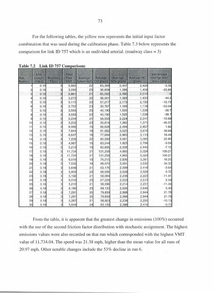
73
For the following tables, the yellow row represents the initial input factor
combination that was used during the calibration phase. Table 7.3 below represents the
comparison for link ID 757 which is an undivided arterial. (roadway class = 3)
Table 7.2 Link ID 757 Comparisons g - ~~4 s ~ . .
_ ~.~ ~_~E'
_ _
~ 3
~' Z ~ --Y- z4-~ ~-
- _ _ .-~'-
~_~ y_
-~c~e.-~~ _ _ ~ 3
--sue_ -~_
.~~ ~'
r
'
- ~
-~
_~ ~ i
-'-
__. ~~, _-~_
_
~ "fit"' ~ ~__
_
~#'s'-~ ~` ~ S 'L,R S _ _ -a4_~`.
fi r. _ _rte. ,~
-
~
~~ -~ _~
__
~~~~vAF. _ _ _
- __
_
_
_ = 3z - .~_
-c'i~=sue- _ _ _ _
=~~
_ ,~=_ 4 _ ___ _, _
_ _ -_ ~ .?-
~_ q-~ g _
'- ~ _
333 _
~. - -chi - ~ ~~~
8 ~
~-, _f :cl £!
~~~
-.~_~
~x'F' S c ~~ ~j g' - - ~ -- - - -_
_ ~~-
~ .~ _ '5==2_~
. ~~-a~~~~~ ~i2
1 0.18 _: _ . .. ~
3 -~~i~'
3F =_ _. . ~?:
5, 665 ~ _ =-f.-_- .._...=s`- _ _r_
22 _
'--~_. . __ _ _-s
63, 366 _ _ _ _.. _ _
2, 407 :_ E _ .. _ r .:ter_._ ~. _... ~'"
2, 426 _
_. .. _ .... .s-__ _~
-3.35 2 0.18 3 3,290 25 36,808 1,398 1,409 -43.86 3 0.18 3 5,861 21 65,562 2,49Q 2,510 0 4 0.18 ~ ~ ~ ~ 3 3, 270 25 36, 581 1, 389 1, 400 -44.2 5 0.18 3 5,115 20 57,217 2,173 2,190 -12.73 6 0.18 3 2, 752 23 30, 787 1,169 1,178 -53.04 7 0.18 3 3,593 23 40,190 1,526 i ,538 -38.7 8 0.18 3 3, 593 23 40,190 1, 526 1, 538 -38.7 9 0.18 ~ v.. y.. ..~... 3
~~ 5,234 ~ 21 58,553 2,224 2,241 -10.69
10 0.18 3 3,202 23 35,814 1,360 1,371 -45.37 11 0.18 3 6,085 15 66,628 2,494 2,457 1.62 12 0.18 ~~ 3 7, 844 18 91, 682 3, 520 3, 674 39.84 13 0.18 3 6,647 16 77,684 2,983 3,113 18.49 14 0.1.8 3 7, 205 22 80, 593 3, 061 3, 085 22.93 15
_ 0.18
_ 3 4, 987
_ 15 63, 244 1, 923 2, 706 -3.54
16 0.18 3 5,210 15 60,895 2,338 2,440 -7,12 i 7 0.18 3 11,734 21 131,259 4,985 5,024 100.21 i 8 0.18
_ 3 11, 734 21 131,259 4, 985 5, 024 100.21
19 0.18 3 6,010 15 76,215 2,936 3,261 16.25 20 0.18 3 7, 535 18 88, 070 3, 381 3, 530 34.33 21 0.18 3 5,648 21 63,176 2,399 2,418 -3.64 22 0.18 3 5, 903 23 66, 036 2, 508 2, 528 0.72 23 0.18 3 5,192 21 58,084 2,206 2,223 -11.41 24 0. i 8 3 6, 010 23 67, 226 2, 553 2, 573 2.54 25 O.i8 3 5,212 21 58,298 2,214 2,231 -11.08 26 0.18 3 6,180 23 69,133 2,626 2,646 5.45 27 0.18 3 7, 291 25 79, 839 2, 988 2, 944 21.78 28 0.18 3 7,291 25 79,839 2,988 2,944 21.78 29 0.18 3 5,267 21 58,923 2,238 2,255 -10. i 3 30 0.18 3 5,644 24 63,130 2,398 2,416 -3.71
From the table, it is apparent that the greatest change in emissions (100°10) occurred
with the use of the second friction factor distribution with stochastic assignment. The highest
emissions values were also recorded on that run which corresponded with the highest vMT
value of 11,734.04. The speed was 21.38 mph, higher than the mean value for all runs of
20.97 mph. Other notable changes include the 53 °10 decline in run 6.

74
The following table shows link ID 1286 that is a collector. (Roadway class = 4)
Table 7.3 Link ID 1286 Comparisons
e e- ~~ ~ .. _ ~ '~~
~ E~ _ _,. _ ~_
~-t o .. •rte-~"' ~+
r
- ~}
1
~~~~~. ~~
s
__
_ Vi c_ __mac ~
,,3 $ ~ ~ ~ ~ T'''"'
_
£~
_ _ -
tr
y__
~~ ~
_ __- ~
._~ -- _~_ ~ d res
'~ ~
_ T_ ~ _`.y
1 ._~__=a..
0.24 ~ 7 T.c,_= . .
4
_sue ___>cy _
1677 -y ~ # r
26 4i
28541
Lz~~ 3
1068
`.
1052
-c~
-7.88 2 0.24 4 2829 31 18373 679 646 -40.7 ~ 0.24 4 169Q 26 30983 11 f 0 1142 9 4 0.24 4 2061 31 18519 684 651 -40.23 5 0.24 4 1657 24 23056 876 8$3 -25.59 6 0.24 4 1414 27 18141 679 669 -41.45 7 0.24 4 1414 27 15485 580 571 -50.02 8 0.24 4 2209 27 15485 5$0 571 -50.02
9 0.24 4 1497 24 24706 938 946 -20.26 10 0.24 4 2286 27 16396 614 605 -47.08 11 0.24 4 2735 19 26713 1026 1071 -13.78 12 0.24 4 24i 5 24 30595 1162 1171 -1.25 13 0.24 4 3320 22 27011 1026 1034 -12.82 14 0.24 4 2500 26 36352 1361 1340 17.33 15 0.24 4 2721 20 31706 1051 1357 2.33 16 0.24 4 2302 22 30440 1156 1165 -1.75 17 0.24 4 2302 26 25203 943 929 -18.66 18 0.24 4 2510 26 25203 943 929 -18.66 19 0,24 4 2582 20 28082 1067 1075 -9.36 20 0.24 4 2224 24 28886 1097 1106 -6.77 21 0.24 4 2621 25 24357 912 898 -2 i .39 22 0.24 4 2528 29 28699 1074 1058 -7.37 23 0.24 4 2390 26 27685 1036 1021 -10.64 24 0.24 4 1400 30 30304 1167 1297 -2.19 25 0.24 4 2757 25 17750 684 760 -42.71 26 0.24 4 2028 29 30187 1130 1113 -2.57 27 0,24 4 2028 31 22218 821 781 -28.29 28 0.24 4 2428 31 22218 821 781 -28.29 29 0.24 4 2571 26 26586 995 980 -14.19 30 0.24 4 0 29 28152 1054 1038 -9.14
Unlike the case for the previous link, the largest change occurred between the base
case and runs 7 and 8 which corresponded to friction distribution 1; assignment technique
stochastic with and without feedback looping. As with the previous case however, the greater
emissions corresponded to higher VMT and average speed values, which is generally
expected from modeling theory.
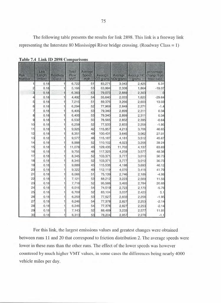
75
The following table presents the results for link 2898. This link is a freeway link
representing the Interstate 80 Mississippi River bridge crossing. (Roadway Class = 1)
Table ?.4 Link ID 2898 Comparisons
~~ -- --n--~~ - ~ - .~ q ~~gg $
_ _ __ _ : _ -~ ~_ __ _ _- - f -~ _ IF'~~.
_~ - -- ..~-,._~.
1 ,~ ,_cam
0.18 k
1 _
-~
6,722 ..
51 83,271 ,
3,043 .. Ti ... -nT~+F3.f
2,425 v . X30 _
5.31 2 0.18 1 5,166 53 63,994 2,338 1,864 -19.07
0.1:8 _ . . ~_ .. ~ 6,383 _ _ _ 53 . _ _.79,073 __ _ 2,889 ., _ 2,33 0 4 0.18 1 4, 492 54 55, 640 2, 033 1, 620 -29.64 5 0.18 1 7, 215 51 89, 376 3, 266 2, 603 13.03 6 0.18 1 6, 294 52 77, 969 2, 849 2, 271 -1.4 7 0.18 1 6, 405 53 79, 340 2, 899 2, 311 0.34 8 0.18 1 6, 405 53 79, 340 2, 899 2, 311 0.34 9 0.18 1 6, 532 50 78, 565 2, 852 2, 395 -0.64
10 0.18 1 6,259 52 77,533 2,833 2,258 -1.95 11 0.18 1 9, 925 42 i 15, 957 4, 213 3, 706 46.65 12 0.18 1 8,351 49 100,431 3,645 3,062 27.01 13 0.18 1 9,577 48 115,187 4,181 3,512 45.67 14 0.18 1 8, 888 52 110,102 4, 023 3, 206 39.24 15 0.18 1 11,078 43 129,435 11,702 4,137 63.69 i 6 0.18 1 9,755 48 117,325 4,259 3,577 48.38 17 0.18 1 8,345 52 103,371 3,777 3,010 30.73 18 0.18 1 8, 345 52 103, 371 3, 777 3, 010 30.73 19 0.18 ~ 9,889 43 115,538 4,198 3,693 46.12 20 0.18 1 9, 322 49 112,119 4, 070 3, 418 41.79 21 0.18 1 6,066 51 75,139 2,746 2,188 -4.98 22 0.18 1 7,121 53 88, 212 3, 223 2, 569 11.56 23 0.18 1 7,716 52 95,586 3,493 2,784 20.88 24 0.18 1 6, 016 54 74, 519 2, 723 2,170 -5.76 25 0.18 1 6,709 52 83,104 3,037 2,420 5.1 26 0.18 1 6,259 53 77,527 2,833 2,258 -1.95 27 0.18 1 6,246 54 77,378 2,827 2,253 -2.14 28 0. i 8 1 6,246 54 77,378 2,827 2,253 -2.14 29 0.18 1 7,143 52 88,489 3,233 2,577 11.91 30 0.18 1 6,313 53 78,204 2,857 2,278 -1.1
For this link, the largest emissions values and greatest changes were obtained
between runs 11 and 20 that correspond to friction distribution 2. The average speeds were
lower in these runs than the other runs. The effect of the lower speeds was however
countered by much higher VMT values, in some cases the differences being nearly 4000
vehicle miles per day.

76
The following table presents the results for link 2830. This link is an arterial link
located on the Davenport Iowa side of the Bi-State area near the Central Business District.
(Roadway class = 3)
Table 7.5 Link ID 2830 Comparisons A
~~'~~vCf~~i~X. ~~F
_~ ~ _ -
~ '
_~
~ ~ ~-
3~r s-.~ r ~ -~i.~
_ -' :~
~ _ '~' _ _
_
- ~..
~.,
_
v
_
~ erg'
T-~_-
_ - :cT-£ .
~~
aa£3
___
~.
'- F
_
~ ~_ Yi ~~F.d~~'~al~
~ ,aces^`
~~-~
~ c~ ~i -_-
xf- y~.r ~_ r
~ ~ _', _'-sue -_ ~'~'_,- ~-~~_. .~'- ~.. ~ gg _ _ _
__ ~_ ~ _ _ z_
_ .__
-
-
~~
_ ~_ _r.= ~'~-~~ _ _
__ter ~. .___. __ ~ __ _ _ ._ ~ . . __ _ _ __ ~. . _ - - ~ ~ ~ ~ _ ~ ~__ ._ ___ _ ~~ - __ . _ r.._._ _ -" ~_.
1 0.6 3 12,101 37 136, 804 4, 977 4, 541 -4.9 2 0.6 3 11,240 39 7 27,071 4,623 4,218 -11.66 3 - 0.6 ~ 12,24 37 -143,851 5,233 4,774 - _ 0 4 0.6 3 10, 683 39 120, 781 4, 394 4, 009 -16.04 5 0.6 3 10,881 35 123,014 4,475 4,083 -14.48 6 0.6 3 10, 856 37 122, 739 4, 465 4, 074 -14.68 7 0.6 3 10, 479 38 118, 471 4, 310 3, 932 -17.64 8 0.6 3 10,479 38 1 i 8,471 4,310 3,932 -17.64 9 0.6 3 10, 846 35 118, 825 4, 390 4,177 -17.4
10 0.6 3 10,554 37 119,320 4,341 3,960 -17.05 11 0.6 3 11, 334 34 124,175 4, 587 4, 365 -13.68 12 0.6 3 13, 806 36 ~ 56, 089 5, 678 5,181 8.51 13 0.6 3 12,592 35 140,858 5,349 5,392 -2.08 14 0.6 3 13, 834 38 156, 398 5, 689 5,191 8.72 15 0.6 3 11,457 34 125,515 2,135 4,412 -12.75 16 0.6 3 13,167 35 144,253 5,329 5,071 0.28 17 0.6 3 12, 807 38 144, 786 5, 267 4, 806 0.65 18 0.6 3 12,807 38 144,786 5,267 4,806 0.65 19 0.6 3 11,490 33 125,877 4,650 4,425 -12.49 20 0.6 3 13,573 36 153,453 5,582 5,093 6.68 21 0.6 3 10,137 38 114, 610 4,169 3, 804 -20.33 22 0.6 3 11,218 39 126,821 4,614 4,209 -11,84 23 0.6 3 10, 694 38 120, 906 4, 398 4, 013 -15.95 24 0.6 3 11, 560 39 130, 693 4, 754 4, 338 -9.15 25 0.6 3 10, 666 37 120, 590 4, 387 4, 002 - i 6.17 26 0.6 3 i 2, 035 39 136, 067 4, 950 4, 516 -5.41 27 0.6 3 10, 695 40 120, 918 4, 399 4, 013 -15.94 28 0.6 3 10,695 40 120,918 4,399 4,013 -15.94 29 0.6 3 9, 964 38 112, 648 4, 098 3, 739 -21.69 30 0.6 3 11, 242 39 i 27, 099 4, 624 4, 218 -11.64
As in the case of the freeway link, the highest overall emissions values were noted for
runs between 11 and 20. (Inverse Function friction factors) In contrast to the freeway link
however, the changes were much smaller with the highest positive change being 8.5%. In
addition, the majority of runs produced declines in emission values. for most of the runs
showing declines, average speeds were between 3 5 and 40 mph with vMT values lower than
the base scenario.

77
The following table presents the results for link 1551, a collector link located on the
Illinois side in Moline. (Roadway class = 4)
Table 7.6 Link 1551 Comparisons
0.25 0.25
4 0.25 0.25 0.25
7 0.25 0.25
9 0.25 10 0.25 11 0.25 12 0.25 13 0.25 14 0.25 15 0.25 16 0.25 17 0.25 18 0.25 19 0.25 20 0.25 21 0.25 22 0.25 23 0.25 24 0.25 25 0.25 26 0.25 27 0.25 28 0.25 29 0.25 30 0.25
4 2, 252 33 24, 671 9 i 1 867 -0.55 4 2,304 38 26,048 948 865 5
.2,264 33 24,808 _ 91 fi 872 0 4 2,330 37 26,342 958 874 6.18 4 2,121 30 23,233 858 817 -6.35 4 1,988 33 21,783 805 766 -12.19 4 1, 982 34 21, 719 802 763 -12.45 4 1, 982 34 21, 719 802 763 -12.45 4 1, 981 32 21, 706 802 763 - i 2.5 4 1,371 34 15,015 555 528 -39.48 4 2,261 30 24,753 927 913 -0.22 4 2,558 34 28,022 1,035 985 12.95 4 2,229 32 24,423 902 858 -1.55 4 2, 510 37 28, 381 1, 032 942 14.4 4 2,193 30 24,010 1,046 885 -3.22 4 2,278 31 24,960 922 877 0.61 4 2,457 36 27,77fy 1,010 922 11.96 4 2, 457 36 27, 776 1, 010 922 11.96 4 2,206 31 24,166 893 849 -2.59 4 2, 263 34 24, 796 916 872 -0.05 4 2,129 35 23,327 862 820 -5.97 4 2,236 38 25,282 920 839 1.91 4 1, 979 35 22, 368 814 742 -9.83 4 2,242 38 25,347 922 841 2.17 4 1, 997 34 21, 879 808 769 -11.81 4 2,400 37 27,137 987 901 9.39 4 2,433 39 27,510 1,001 913 10.89 4 2, 433 39 27, 510 1, 001 913 10.89 4 1,839 36 20,786 756 690 -16.21 4 2,044 38 23,107 841 767 -6.86
Following the general trend of the previously studied links, the highest emission
values were observed in the runs between 11 and 20. Of note however are the high values for
runs 27 and 28 which are Stochastic (feedback and non feedback cases). In all cases where
emissions are high, the VMTs and average speeds per run are correspondingly high.

~g
The following table presents the results for link 1131, a freeway link representing the
Interstate 74 Mississippi River bridge crossing. (Roadway class = 1)
Table '~.7 link 1131 Comparisonsr _._ s _~ - -~ ~~- - - ~- -- -
~ rt~_ ~ -~= -~ -
' ~ _ - _ ,' ~
- - - _ - ~_ -_ s - - _ _
~_~ -- _~ _ _ - _~ ~_~_-.- --~ -"~ -. Vii,=. ~ _ '"'
~=. i _sa ~
_ r~
.z- ,ter - ~~ -_
_
~_,
_ __ Y ~
..-._ - - __ _
-~
.. _ c
s
a-~ _
_^x. -x _._ - _ ~z~
_.~.. ~ ._ . ~,.". a ggg
5 g~'
~t
~
- _ _ . - .sue - ~ ~- ' _
'~ _~
~ ^ {
_
=~_ -_
~~ 1- _ _ __
__ _ _ _
__ F`
[Y_
- - _ .. _
.. r
1 0.37 1 29,179 46 350,927 12,737 10,699 1.22 2 0.37 1 i 4, 779 50 183, 079 6, 690 5, 332 -47.86 3 0.3? 1 28,827 46 346,697 12,584 i 0,570 d 4 0.37 1 14, 817 50 183, 540 6, 706 5, 345 -47.73 5 0.37 1 27, 735 ~ 44 324, 042 11, 774 10, 358 -4.99 6 0.37 1 15,181 47 182, 574 6, 627 5,566 -47.34 7 0.37 1 14, i 89 48 170,655 6,194 5,203 -50.78 8 0.37 1 14,189 48 170,655 6,194 5,203 -50.78 9 0.37 1 27, 289 43 3 i 8, 834 i 1, 585 10,191 -6.52
10 0.37 1 15, i 40 47 182,083 6,609 5,551 -47.48 11 0.37 1 28,249 34 314,755 11,646 11,087 -3.93 12 0.37 1 37,583 38 426,829 15,636 14,332 27.65 13 0.37 1 31,760 36 360,698 13,213 12,112 7.87 14 0.37 1 41,416 43 483,886 17,582 15,467 41.87 15 0.37 1 27,066 34 301,578 6,387 10,623 -20.59 16 0.37 1 28, 766 35 407, 585 14, 837 18, 942 38.22 17 0.37 1 37, 931 43 443,164 16,102 14,165 29.93 18 0.37 1 37, 931 43 443,164 16,102 14,165 29.93 19 0.37 1 27,941 35 311,325 11,519 10,966 -4.97 20 0.37 1 37,046 38 420,725 15,412 14,127 25.83 21 0.37 1 27,315 44 319,137 11,596 10,201 -6.43 22 0.37 1 30,373 48 365,296 i 3,259 11,137 5.36 23 0.37 1 27,473 44 320,980 11,663 10,260 -5.89 24 0.37 1 30,417 48 365,817 13,278 1 i ,153 5.51 25 0.37 1 27,341 44 319,446 11,607 10,211 -6.34 26 0.37 1 30,718 48 369,441 13,409 11,263 6.56 27 0.37 1 33,804 50 418,752 i 5,301 12,195 19.25 28 0.37 1 33, 804 50 418, 752 15, 301 12,195 19.25 29 0.37 1 26,411 44 308,571 11,212 9,863 -9.53 30 0.37 1 30, 512 48 366, 958 13, 319 11,188 5.84
The VMT and emissions values were highest between runs 11 and 20. In addition, the
absolute value of the percentage changes was also high in this range. The largest percentage
change was an approximately 50°Io decline from the base situation when the Stochastic
assignment technique was utilized. (Runs 7 and 8) The average speeds were lower in runs 11
- 20 than between runs 1 - ~0 and 21 - 30 and indicate some measure of congestion on the
bridge when friction distribution 2 is applied.

79
The following table presents the results for link 2648, a freeway link representing the
Interstate 80 in the Western sector of the model. (Roadway class = i)
Table 7.8 Link ID 2648 Comparisons ~_,~ -' sue ' -~'-~~_ °'~=~ ~ ~ "~ ~ ~'~'c` ~-~_-~~~" z - ~. r - ~ ~: _ `~~_ ~"~ ~ ~~'.
'tc _- ".'.~"~"`'~ ~ ~=fig __ r
~~~ _y~=~~~~`~'_ ~ _
G~~~ ~._-= _ =-~~~ - --~ ~_
est ~s.~
~ :. ~#~_~~~`~`~~`~ _ -~ 3~~
^{~ a'€.e ~.a'~ ,e'=
--- ~~. ~~__
~~.~~.; '- y~~ ~.- _ j ..~ t~
_ - ' ...;~~
_ ~- ._ - -ate ~ _
;1~ rs~
~ 1~ ~
_
Ems SPF +~i ~ Ra E
~~ ~ _s- _
-'i~3 :'~_~. _= l y
___~'axc~ =-rz_+.i3_'~`'~._.~ -
v. :. .',.'..~'c_-s_ Y~F - .?-_, ~_ '311F .. _.~>.~._.= ..c_. ..-:? __._ s.-~. .,...< ._ ._ _ ~~- =+.s"~.:-~~- ~ 2._ ___ ._._.-l.__ _. __... _-.x_._. _ _
c
_
.
...._ v
g._~g
__ ...,'a§+t~ ~.v_,. .~.rc--r.r-~
..-~~
.,. .~ _.
1 2.61 ~ 143, 435 54 1, 776, 807 64, 923 5 i , 746 0 2 2.61 1 142,475 60 1, 821, 858 67, 51$ 50, 851 1.6 3 2:61 ~ 1.43,435 54 1,776, 8{~7 ~4, 92 t 51, 746 4 2.61 1 142, 475 60 1, 821, 858 67, 518 50, 851 1.6 5 2.61 1 143,435 49 1,725,081 52,61 ~ 52,593 -1.61 6 2.61 1 142, 475 54 1, 764, 905 64, 488 5 i , 399 -0.67 7 2.61 i 142,475 57 1, 821, 858 67, 518 50, 851 1.6 8 2.61 1 142, 475 57 1, 821, 858 67, 518 50, 851 1.6 9 2.61 1 143,435 49 1,725,081 62,614 52,593 -1.61
10 2.61 1 142,475 54 1,764,905 64,488 51,399 -0.67 11 2.61 i 143, 435 52 1, 776, 807 64, 92 51, 746 0 12 2.61 1 143,435 57 1, $34,144 67, 97 ~ 51,194 2.29 13 2.61 1 143, 435 54 1, 776, 807 64, 923 51, 746 0 14 2.61 1 143, 435 60 1, 834,144 67, 97 ~ 51,194 2.29 15 2.61 ~ 1 143, 435 51 1, 776, 807 31, 550 51, 746 -6.13 16 2.61 1 143, 435 54 1, 776, 807 64, 923 51, 746 0 17 2.61 1 143,435 60 1, 834,144 67, 97 ~ 51,194 2.29 18 2.61 1 143, 435 60 i , 834,144 67, 97 ~ 51,194 2.29 i 9 2.61, 1 143,435 51 1,776,807 64,923 51,746 0 20 2.6 i i i 43, 435 57 1, 834,144 67, 97 ~ 51,194 2.29 21 2.61 1 143, 435 54 1, 776, 807 64, 923 51, 746 0 22 2.61 1 143,435 60 1, 834,144 67, 97 ~ 51,194 2.29 23 2.61 1 143, 435 54 1, 776, 807 64, 923 5 i , 746 0 24 2.61 i 143, 435 60 1, 834,144 67, 97 ~ 51,194 2.29 25 2.6 i 1 143,435 54 1, 776, 807 64, 923 51, 746 0 26 2.61 1 143, 435 60 1, 834,144 67, 97 ~ 51,194 2.29 27 2.61 i 143, 435 63 1, 896, 665 72, 031 50, 870 5.33 28 2.61 i 143,435 63 1, 896, 665 72, 031 50, 870 5.33 29 2.61 1 143,435 54 1,776,807 64,923 51,746 0 30 2.61 1 143, 435 60 1, 834,144 67, 97 ~ 51,194 2.29
Unlike the previous comparisons, the changes on this link were very small. There was
no percentage change greater than 7%. This is possibly explained by the fact that the link
represents the western departure from the model of Interstate 80. Consequently, the influence
of the sensitivity runs was diminished given that a greater proportion of the trips are external,
the OD values of which were not varied during the sensitivity runs.
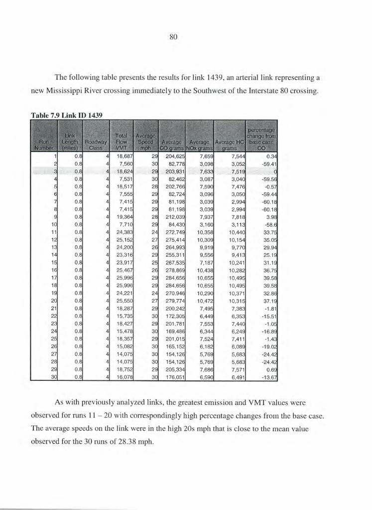
80
The following table presents the results for link 1439, an arterial link representing a
new Mississippi River crossing immediately to the Southwest of the Interstate $0 crossing.
Table 7.9 Link ID 1439 __ _ _ a~ ~
a ~'~
~
~~
_ _ ~ _ ~~
y-~~¢
:.~
"tee:: ~,~''` a
~- s: ._'a .,,.
r, ~ - _
~ 'fi x~'~~'~ s
~
-
~ ~
~
~
~ ~-`~-' ~
_ - _ _- __:~_,~~=s_.= =-F~a~`~
t~s ~ ..e ~. ~,~ ~a'3 ~ ~
~" ~ 55~ ''~ ,"tf,~..~-
~~ic~""~i i ~
~ ~
~
-L'~" _fig+_ ~~
-}s ~ 9F' ~? - ~R~
T g3 ~ x~"_~' '.z~~i.
_ _~.ad .. Fs' ~${~eF_ =
-sue' +
S. 3 = -~
-
~
~~ 'L __... ~f ~ ~a ~
q~ a -.-~ .~
~~- _ _ T_
_- Ee:~~ C~i~x~i f
_
r
g
_ ~
_ - F Ee..3 F - ~
_ ~- EE
..~
~~ ~ rt $-~
__~ 4 _a~rvc~~
.# 3
-3~3_~ .. -~ t -L "'4.~~1i ~Y"_~ _ -' ~~- a-1 ~~Y __'~-~~~ _ ~_~ ~y~~
_ _ ~._ ~_-._. _-~.
s ~ 3P
~--~•aaG" __. _ -mss .. .__ ._ - _ ~?t~S°i ~ ._ _. :., _._..-p- _:
3 - ~~ _... xz-
a: .. ~ ~ ____
_ _ _ ~~s __¢` ¢'~$~'~'R
,... __ `y
_ a _ c ~~iTS
v~ Q . ~ __ ~ 3c-
~~',~. ~~rs. _.__
~._ d~ __
'mr-.-_ y' --
1 0.8 4~ 18, 687 29 204, 625 7, 659 7, 544 0.34 2 0.8 4 7, 560 30 82, 778 3,09: 3, 052 _ _ __ -59.41 ~- 0.8 4 - 18,624 29 203,931 7,633 7,51 ~ 4 0.8 4 7, 531 30 82, 462 3, 087 3, 040 -59.56 5 0.8 4 18, 517 28 202, 766 7, 590 7, 476 -0.57 6 0.8 4 7,555 29 82,724 3,096 3,050 -59.44 7 0.8 4 7, 415 29 81,198 3, 039 2, 994 -60.18 8 0.8 4 7,41 5 29 81,198 3,039 2,994 -60.18 9 0.8 4 19,364 28 212,039 7,937 7,818 3.98
10 0.8 4 7,710 29 84,430 3,160 3,113 -58.6 11 0.8 4 24,383 24 272,749 10,358 10,440 33.75 12 0.8 4 25,152 27 275,414 10,309 10,154 35.05 13 0.8 4 24, 200 26 264, 993 9, 919. 9, 770 29.94 14 0.8 4 23, 316 29 255, 311 9, 556 9,413 25.19 15 0.8 4 23,917 25 267,535 7,187 10,241 31.19 16 0.8 4 25,467 26 278,869 10,438 10,282 36.75 17 0.8 4 25, 996 29 284, 656 10, 655 10, 495 39.58 18 0.8 4 25, 996 29 284, 656 10, 655 10,495 39.58 19 0.8 4 24,221 24 270,946 10,290 10,371 32.86 20 0.8 4 25,550 27 279,774 10,472 10,315 37.19 21 0.8 4 18, 287 29 200, 242 7, 495 7, 383 -1.81 22 0.8 4 15,735 30 172,305 6,449 6,353 -15.51 23 0.8 4 18, 427 29 201, 781 7,553 7, 440 -1.05 24 0.8 4 15,478 30 169,486 6,344 6,249 -16.89 25 0.8 4 18,357 29 201,015 7,524 7,411 -1.43 26 0.8 4 15, 082 30 165,152 6,182 6, 089 -19.02 27 0.8 4 14,075 30 154,126 5,769 5,683 -24.42 28 0.8 4 14, 075 30 154,126 5, 769 5, 683 -24.42 29 0.8 4 18,752 29 205,334 7,686 7,571 0.69 30 0.8 4 ~ 6, 078 30 176, 051 6, 590 6, 491 -13.67
As with previously analyzed links, the greatest emission and VMT values were
observed for runs 11 - 20 with correspondingly high percentage changes from the base case.
The average speeds on the link were in the high 20s mph that is close to the mean value
observed for the 30 runs of 28.3 8 mph.

81
The remaining 12 tables are presented in Appendix F. From the tables, it can be seen
that the highest emissions values occurred on freeway links. It was also observed that for
most of the links analyzed, the largest changes occurred on the runs using the second friction
factor distribution {Inverse Function). The following table illustrates the mean vMT,
emission and speed values for each run over all selected links.
Table 7.10 All Selected Linl~s
1 2 3 4 5 6 7 8 9
10
11
12
13
14
i5
16
17
18
19
20
21
22
23
24
25
26
27
28
29
30
~. -~ }~_. 0.18 20,391 40 0.18 16,711 42 0.18 ~0, 353 40 0.18 16,387 42 0.18 20, 742 39 0.18 17,313 41 0.18 17,500 41
41
39
4i
0.18 ~ 22, 896 36 0.18 23,153 39 0.18 23,163 37 0.18 22, 945 41 0.18 23,686 36 0.18 23, 533 37 0.18 22, 956 41 0.18 22, 967 41 0.18 23,144 36 0.18 23, 666 39 0.18 19, 724 40 0.18 19, 805 42 0.18 20, 333 40 0.18 19,309 42 0.18 20, 015 40 0.18 19, 360 42 0.18 19, 238 43 0.18 19,258 43 0.18 20,243 40 0.18 19,475 42
0.18 17, 540 0.18 20,414 0.18 17, 292
250,237 210,246 250,651 206,700 250,940213,872 218,471
9,196 7,470 7,809 6,003 9;234 7,457
7,680 5,901 9, 204 7, 645 7, 869
218,471 246, 947 212,999 274,671 284, 935 280, 688 284, 349 284, 779 289, 895 283,196 283,196 278,361
8,084 8,084 9, 061 7, 839
10, 084 8, 51 i 10,532 8,508 10,323 8,553 10,520 8,393 6,650 8,856
10, 646 9, 077 10,478 8,397 10, 478 8, 397 10,220 8,638
6,294 6, 340 6,340 7,538 6,271
-0.14 - i 7.02
0 -18.41
0.77 -i 5.02 -13.43 -13.43. -0.76
-15.35 10.97 13.94 12.82 13.3 1.46
17.55 13.02 13.02 12.52
291,346 10,765 8,695 i 6.47 241,154 8, 865 7, 206 -3.72 248,354 9,217 7,182 -1.6 248,938 9,147 7,436 -0.64242,905 9,020 7,037 -3.69 244, 350 $, 982 7, 301 -2.45 243,119 9,025 7,034 -3.65 243,944 9,136 6,952 -3.51 243, 944 9,136 6, 952 -3.51 247, 650 9,101 7, 400 -1.14 245, 712 9,122 7,111 -2.61

82
Average vehicle miles traveled on selected links per sensitivity run
a ~, 23, 000 •— ~ ~~ ~ ~, 21,000 .0 ~
~ a 19 000 ~_ , a, ~- ~ ~ ~ 17, 000
1 3 5 7 9 11 13 15 17 19 21 23 25 27 29 Run number
Figure 7.7 Vehicle Miles Traveled per sensitivity run
CO
Em
issi
ons
(gra
ms;
300, 000 - 290,000 280, 000 270, 000 260, 000 250,000 240, 000 230, 000 220, 000 210, 000 200,000
Average CO Emissions for selected links per sensitivity run
T ~ T 1 3 5 7 9 11 13 15 17 19 21 23 25 27 29
Run number
Figure 7.8 Average CO Emissions per sensitivity run
VMT
CO

83
Average NOx and HC Emissions per Sensitivity run for selected links
12,000 -
__ 11, 000
~ 10, 000 L
~ 9, 000 ...
.° 8, 000
'~ 7, 000 W
6, 000
5,000 T T T - i-- T 1
1 3 5 7 9 11 13 15 17 19 21 23 25 27 29
Run number NOx HC
Figure 7.9 Average HC and NOx Results for Selected Links
10 -
5
0 0 a~ _ -5 t V
X10
as a -15
-20
-25 -
Percentage Changes of Speed, Emissions and VNIT from Baseline Case (Bi-State Friction Factors)
:«~T
FT~'
I Ali ~
+ I
+Fl!?
■
~~
~~
~
E ._ L
.~
W
c r
L V
cva W
V 0
o E=mi:~sions
® VM1~
o S peed
Figure 7.10 Percent change from Baseline for Speed, Emissions ar►d VMTs for selected cases (Bi State Friction Factors)

84
Percentage Changes of Speed, Emissions and VMT from Baseline Case (Inverse Function Derived
Friction Factors)
~ Ernissions
~ V I'JI T
o S ~>eed
Figure 7.11 Percent Change for Speed, Emissions and VMT from Baseline (Inverse Function Derived Friction Factors)
20 -
15 -
a~ 10 - a~ c co V 5-c as a~ 0 a
-5
Percentage Changes of Speed, Emissions and VMT from Baseline Case (Gamma Function Derived
Friction Factors)
•~-Q
U
-10 -
t
c~
U
.~
W L V
_~
v
~. ~~
Lll
v ®Emissions
~ VMT
o S peed
Figure 7.12 Percent Change for Speed, Emissions and VMT from Baseline (Gamma Function Derived Friction Factors)

85
CHAPTER 8. ANALYSIS OF RESULTS
STATISTICAL ANOVA
The basic task being undertaken in this research is a comparison of the results of a
response variable (NOX, VOC and CO pollutant levels) over categories of three explanatory
variables. The basic statistical tool used to compare the means of groups is the difference in
means t-test. In such atest, a t-statistic for the group differences is calculated and used via a
lookup table to obtain the P-value. Analysis of Variance (ANOVA) represents a
generalization of the difference in means t-test where two or more groups can be compared.
In fact, the resulting F test statistic for an ANOVA with two groups and one explanatory
variable is equivalent to the square of the t-statistic for the t-test. F = t2. (27, 28) The t-test
statistic is shown below.
t = ~y ' - }~ z ~ where n is large (> 30) (27, 28) z z si s2
ni n2iZ 1 Yl 2
where y ~ =the mean for group 1
y 2 =the mean of group 2
s ~ = sample standard deviation of group 1
s2 =sample standard deviation of group 2
nl =number of samples in group 1
n2 =number of samples in group 2
In addition to comparing dependent variable results over categories of one
explanatory factor, multi-factor ANOVA can be employed to compare results for multiple
explanatory factors. Each factor is tested independently while automatically controlling for
the effects of the other factors. This technique allows for rapid identification of the

86
significant factors and any significant interacting effects between the factors by obviating the
need to individually compare two factors at a time using one-factor ANOVA.
ANOVA ANALYSIS OF INPUTS
Following the use of the univariate GLM (General Linear Model) procedure in SPSS
to perform multi-factor ANOVA, it was concluded that at least one of the input factors had a
statistically significant effect on the output emissions. The following hypothesis test was
used to arrive at such a conclusion.
ANOVA Assumptions (1) Population distribution of the emissions is normal. (2) Population Standard deviations (variances) of each group are equal.
SPSS histograms were used to check the assumption of normality for the distribution
of emissions results over all sensitivity runs.
Histogram of Emission Values for
Link/Run Combination
X Y C
100000
80000
60000
40000
20000
- - - - - - - - - - - - - - - 7 ~ 7 7j 7 7 7 7 7 7~ 7 7
~o ~o ~o ~o ~o ~o ~o ~o ~o ~ ~b~ ~~ ~ ~ ~b ~ ~b
Link Emissions (g)
Figure 8.1 Frequency distribution of emissions values

87
From the histogram above, it was apparent that the emissions data were not perfectly
normally distributed. This is not surprising given that in many urban areas, larger roadways
carry a disproportionate share of the total traffic. Consequently, it was decided to modify the
data by taking the cube root of emissions to get a more normally distributed dataset. This
technique is accepted practice in many statistical situations and still allows meaningful
conclusions regarding factor effects to be drawn about the group differences despite lower
absolute values. (29) The order of the differences between input factor combinations will
thus be unchanged for the cube root of emissions allowing the same conclusions to be drawn. The following illustrates the modified distribution, which is now approximately normal in character.
Histogram of Modified Emission Values for
Link/Run Combination
Li n k
X R
u n C
ount
12 16 20 24 28 32 36 2 6 10 14 18 22 26 30 34
Link Emissions (g)
Figure 8.2 Frequency distribution of modified emissions values
For the equality of variances assumption, SPSS provides a test called Levene's test, which is simply an ANOVA on the model variances instead of the model means. The results

88
of Levene's test are displayed along with the ANOVA result table. If the variances are found
to be non-homogenous (not equal), several methods may be applied to rectify the problem.
They include: (29)
1. Trimming data of outlying values.
2. Transforming the data (similar to procedure done above by getting the cube root of
the emissions values).
3. Using ANOVA corrections.
4. Using a distribution free ANOVA test such as the Kruskall-Wallis or Friedman test
where no assumptions are made regarding data normality and variances.
HYPOTHESES:
Ho: mean emissions value for all runs is equal
Ha: At least one mean from the set of runs is different.
Table 8,1 Between-Subjects Factors
firs# friction run 2nd friction run 3rd friction run no feedback Feedback Capacity Restraint User Equilibrium Incremental Stochastic Stochastic User Equilibrium
30590 30590 30590 45885 45885 18354 18354 18354 18354
18354
Table 8.2 Tests the null hypothesis that the error variance of the dependent variable is equal across groups. Levene's Test of Equality of Error Variances Dependent Variable: NEWEMM F df1 df2 Sig.
8.21 29 91740 0+ {Yes)

89
used on the results from the Levene's test, it can be concluded that at the lO~Io
significance level, the variances between groups cannot be said to be equal. The calculated F-
value was 8.205 ivin a P-value ~ 0+ for df~ = 29 and df2 = ~ where df = de reel of g g g
freedom. Given this fact, it was necessary to use method number 3 described above to correct
for the situation. The technique used was to modify the P-value supplied by SPSS to a more
conservative value by using lower degrees of freedoms for given F-values. This approach
will lower type I errors at the expense of increased risk of type II errors. Type I errors refer to
the probability that we conclude that a factor is not significant when it is in fact significant.
Type II errors are the opposite condition; the probability a conclusion is made that a factor is
not significant when it is in fact significant. To make the P-values more conservative than
those given, a good strategy was to find the critical F-value at 1, n-1 degrees of freedom. (29)
Using such a strategy, for any given P-value to be significant, a much larger (and thus more
conservative) value of F would be required. From the table above without corrections, it
could be concluded that all the input factors and their associated interactions were significant
at the Salo significance level. Applying the technique described above to make the results
more conservative gave the following table.
Table 8.3 ANOVA Table With Corrections for non Constant Variance Tests of Between-Subjects Effects
Dependent Variable: NEWEMM -, _
~ ~.`~~. 3^. ~_' 3 ~ -t .~_ mss . ~~' ~
-s^ -~ _~ ~~~~~ffi =g ~ "mil ~ -.. ~_ _ j ~-'~# --z . ~ ~~ y --- -- ~
ye~f a; ~ ~ ea` _ -'--
Corrected Model 13516.45 ~ 1 466.08461 30.257389 0.000+ Yes Intercept 7342180.5 1 7342180.5 476641.39 0.000+Yes FRICTION 6369.8973 1 3184.9486 206.76124 0.000+Yes FEEDBACK 1007.9962 1 1007.9962 65.437333 0.000+ Yes ASSIGN 3406.3481 1 851.58704 55.283526 0.000+ Yep
FRICTION FEEDBACK 1686.7964 i 843.39821 54.751922 0.000+ Yes
FRICTION ASSIGN 365.06635 1 45.633294 2.9624328 0.0852 No
FEEDBACK* ASSIGN 252.89239 1 63.223097 4.1043318 0.0428 Yes
FRICTION FEEDBACK* ASSIGN 427.45677 1 53.432096 3.4687173 0.0625 No Error 1413162.3 91740 15.403993 Total 8768859.3 91770

90
Using this modified table, it could be seen that all input factors were statistically
significant at the a = 0.05 level. However, some of the interactions were determined to be
non-significant including the 3rd order interaction. Given that all input factors were found to
be significant, further analysis was required to determine which factors and interactions had
the largest effect.
E~:AMINING THE FRICTION/FEEDBACK INTERACTION EFFECT
In ANOVA analysis, the normal procedure requires the examination of the highest
order interaction effects first, followed by lower order effects if such higher order effects are
not found to be significant. For this situation, the highest order interaction is a 3rd order given
that there are three primary input factors. The corrected ANOVA table however illustrates
that the 3rd order interaction (FRICTION X FEEDBACK X ASSIGN) was not found to be
significant at the a = 0.05 level. Consequently, the three 2nd order interactions were then
evaluated with two being found significant. They included the FRICTION X FEEDBACK
interaction and the FEEDBACK X ASSIGN effect. Profile plots of these significant
interactions were then utilized to draw conclusions regarding their behavior. Illustrated below
is the plot for Friction/feedback interaction.
Friction Factor/ Dynamic Distribution
Plot 9.4
9.2
9.0 ■
8.8
8.6
8.4
8.2
first friction run 3rd friction run 2nd friction run
Friction Factor Distribution
Feedback/No Feedback
®no feedback
®feedback
Figure 8.3 Friction Factor/ Feedback Profile Plot

91
From the plot above, it is clear that particularly between the 1St friction distribution
results and the results for the second that a significant interaction is taking place. There is a
much less noticeable interaction taking place between the second and the third runs. The
interaction can be explained by the fact that the feedback results are directly dependent on
the actual friction factors used. Recalling from Chapter 3, the feedback process involves
performing the trip distribution stage repeatedly using congested network travel times. It thus
becomes clear that any difference in the friction factors will have a direct effect on the trip
distribution results and consequently the traffic assignment and emissions results. The much
larger difference between friction runs 1 and 2 compared to runs 2 and 3 is the result of a
greater difference in the friction factor distributions between runs 1 and 2 than between runs
2 and 3.
For all friction distributions used, the marginal mean emissions values for the
feedback case were larger than were the case without feedback. This is not a surprising
relationship given the fact that when feedback is incorporated in the model, congestion delay
is represented thus increasing average travel times and distances. The proportion of vehicles
traveling at inefficient speeds was thus increased. Given that inefficient vehicle operation
increases emissions for a given distance traveled and more distance was actually traveled, it
was expected that emission values will be greater in the feedback situation.
Feedback Looping /Assignment Plot 9.4
C
9.2 ■
9.0 ■
8.8
_~---~~
t__ ..----~'
~~
Assignment Technique
`-'~,. __,.—E' ~ Capacity Restraint
User Equilibrium
~ Incremental
~ Stochastic
~~ Stochastic User Equi
8.6 librium no feedback
Feedback/No Feedback
feedback
Figure 8.4 Feedback Looping/ Assignment Technique Plot
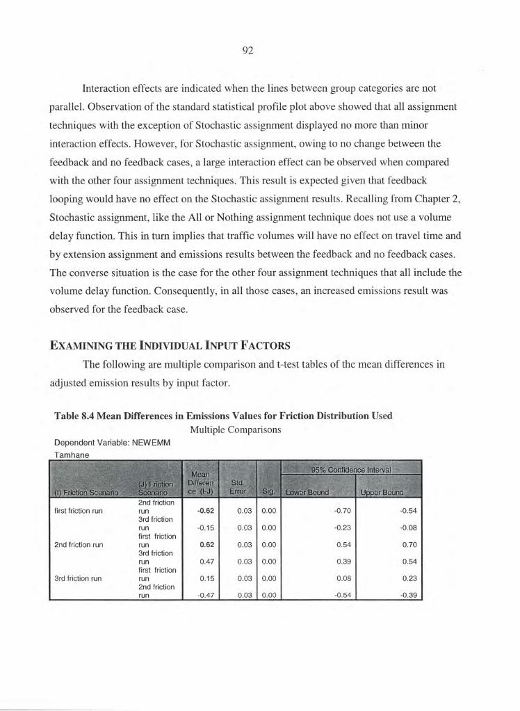
92
Interaction effects are indicated when the lines between group categories are not
parallel. Observation of the standard statistical profile plot above showed that all assignment
techniques with the exception of Stochastic assignment displayed no more than minor
interaction effects. However, for Stochastic assignment, owing to no change between the
feedback and no feedback cases, a large interaction effect can be observed when compared
with the other four assignment techniques. This result iS expected given that feedback
looping would have no effect on the Stochastic assignment results. Recalling from Chapter 2,
Stochastic assignment, like the All or Nothing assignment technique does not use a volume
delay function. This in turn implies that traffic volumes will have no effect on travel time and
by extension assignment and emissions results between the feedback and no feedback cases.
The converse situation is the case for the other four assignment techniques that all include the
volume delay function. Consequently, in all those cases, an increased emissions result was
observed for the feedback case.
EXAMINING THE INDIVIDUAL INPUT FACTORS
The following are multiple comparison and t-test tables of the mean differences in
adjusted emission results by input factor.
Table 8.4 Mean Differences in Emissions Values for Friction Distribution Used Multiple Comparisons
Dependen# Variable: NEWEMM Tamhane ~~~ _ ~ ~ ~, ~ _. ,~:~3~ ~ ~; - _ _ _ ~ _ _ __ _ . ~ . ~~ ~ ~ ~~--~ _~ ~~__ :;~~ ~_ - _ _-- - _ ------~--~~~~~ ~ ~ - - - Tom=-T~ .~ _= - ~ --_=~- _ ~, ~~~ -~- f ~-~-~ _ ~-- Wiz_ - ~ -~- ~ ~ _ ~ -~- --
~~~.- . -~ - -- _- - _- -- _-~- - u ~_
.~-~~3?< -. . x'5;4 'J' F.
, ~j c z
~ _~ ..43'
"'hEr?T_. ~ ~~a'~~~~~~~'l
,3,_- fiat - ;. ~~ 2Y
§ '3'`
.-~~
_ _
_ ~.~_ _ _ _
~ g _ ____
_- ~_^_
__ _ __s -a__ _ -_~_~~ _ _ ~._
__ ~-
_ _ sv--=- ^ ~ i_'_m.~. _ ~.
~~~_
,~ ^~_~_-v~'
a-+" ~~ __~
~~.:L_n3~~=F
_ __
~_ ~_ ~~~ ~., .....„k? 3 L ._~ '~
' ~ -s-j ~: ~~~~i.. -e~
J
-'^df,'c.Y ~ '.r' ~ F . ~: 2 rs
..~k'~~ _
_ _
E
..~~ -_. -
__
-~ ~
~ ~~
_~ - = ~-._
_
'`e_T' ~ -~~x--~ _"_S ~-c_~v'~' ~
~- ~-a-F.-Yc _~T= r~ ~ ~i Vii' ~~~ ~~~ -m`~_' ~~
_ . _ _
first friction run
2nd friction run
3rd friction run
2nd fric#ion run 3rd friction run first friction run 3rd fric#ion run #first friction run 2nd friction run
-0,62
-0.15
O.S2
0.47
0.15
-0.47
0.03
0.03
0.03
0.03
0.03
0.03
0.00
0.00
0.00
0.00
0.00
0.00
-0.70
-0.23
0.54
0.39
0.08
-0.54
-0.54
-0.08
0.70
0.54
0.23
-0.39

93
Table 8.5 Mean Difference t~test for the Feedback/No Feedback Input Factor Independent Samples Test ~~ ____ -. - ~= -~~_--
. _~ _ __
~-
~ _,z~ _ '~'S _ _ _ __ ~~ __ _ a . ' ~~em-_ _ _.~_z'c~__ r ~d?_~
-~ _ Yom _
: ^ -.' -s-s~T'_ __ _ _ ~.._~ ~ ~.~ _ _ ~ -~- 'r-~~ - _ _ _
_ ~-~- -- _ _, _ ~~..`~'~ r " _ --_._cam _~_ _ ~- c - -- ~c~
.~~-^=°c_?~~=,~_~ _ ___~~_ __ z ~
"m -_- '~~''m- ~ 3 ~_ ~ ~ ~ _- ___ _
'~-s+-ne- ~ -_s '~.*~ ~__ _ ~ i_+. .3.ax-'E.~=_ !.Pc t.=~~
-~
-~ ._a __- .r .c_.~
.~ __ .:_~-~~~ ~~ _ _ _ -' _-__ _
~
+F~ ~i=3.s
_
-zr"c'-~"
_
_ _ _ _ 'v} c` v
j,
- _ _ _ __ s
-~ --cE
-~
-- _ __ _J. T -_ - ms s=
__+-.
_
_ _ _ -_ ~~ ~~-
_ -,. ~ __zc _ ~ _ _ _ _
` ~~ ___ _ -_~- ___-~ -YS'v-ax 's. -?-4 _L _
_ ~ _ _ _ ~~
~~'~
c 'c. _
_ _ - _ _ T...~ _- ~_
_'-c~c~~~
L_= ~~ ]R_-_ ____ _ __
_ _- ._ _ 's "'~ scw3
_ ~__ s ___~__ - ~ ~= __a_ -~ "~S_ _ ._.-ate• _ ~ -~_~~. _.
Equal variances NEWEMM assumed
Equa! variances not assumed
_
-8.05
-8.05
_ _ -- __~w~ ~"
91768.00
91747.90
_ _ _ _ ~_
0.00
0.00
.__ _
-0.21
-0,21
-
0.03
0.03
_-'.
-0.26
-0.26
-0.16
-0.16
Table 8.6 Mean Differences in Emissions Values for Assignment Technique Used Dependent Variable: NEWEMM Tamhane ._ ~. . ~ _. _~_ ..~. ~ _ _ _ ~ _ _ ~ _ _ _ _-
~ ~ -v.~' _r
~
_ _ - __ . v~, ~ ~~ .'~~ s-... G v a1 .c~{ c Ti? _~
-~~.r~--~ ~ j' ~J _ _ _`_~.. ti _
. _~__~ ~ _ _ - _`- _ ""' ~~_
J.J. - ~..~
-_ _ - ~_ - ~ ~ ~. 3'~c• G _ __
_ ~
_ _ A ~ _ .. _ . ~ _ .-,+-n.- _ _ _ _ _ _ - _ -_-_ _ _.-__- .''~`''.-__ :.mss _ _ ~~_'~_ - ___~'_~
-~- ~ _ __~g
4~[y-'}gip
$-=e~. _ ~_s ~,_ - ~ _ __"g~ 4~ - ~~~~ ~-T' ~~r
~ ~ . ~E
_ _; ~~~.2~3` cv~+~"'.~~ _ ~a'~_ _ '~-~'~'
-~~FE~-c_.tu~ --
~ - _ _~'_`~. __ s E`$ s ~ = ..~~~ 4 ~~'&~
. -_ a_..n_^ __ -~ _ 3r.~v ~ ~ ~ - .. _. .. a. ~ B. ~t~ : ~ ~ . C : ~... - -r_ _~-~~ --~=._~'
~'~~~- ~ fi x.. ~ ~ ..-i - - ~i "~ ~~-- ~.r~
~_ ~- mod' ~ vr-~' a'~ _ `i~~- :~' ~ _
'2"` E -CF' _. a~F."°~' . ~ _
~,'` x'dv s -. ~ -, _
".- ~ ~ ~~`c~:,- "` ..~.0 .o-~r
n.-r ~--~ _~~~_~~~'~ ~_~~~ u ''`~=?;€3
~- .{"t ..~ ~ v Y - £ ~ ._ _-- _i
~ ~' ~~ ~ ~f '"~_~: ~ __~ ~ 4 ,__.~ - __.. _
_ '_ sl~ f -
. __ _ _. ...-c F2 r.
_ k
; m _ ~ ~~_-s - r
~ _- c --~-- 5-.. ' .~=~-c. :~i
_ y#j~r~. `E! ~+`{ ~i~ ~~r
^=-~~~6~~~~~r.]..... ~~
User ~r~
Capacity Restraint Equilibrium 0.00 0.04 No -0.12 0.12 Incremental -0.01 0.04 No -0.13 0.10 Stochastic -0.50 0.04 Yes -0.61 -0.39 Stochastic User Equilibrium -0.12 0.04 Yes -0.24 0.00
Capacity User Equilibrium Restraint 0.00 0.04 No -0.12 0.12
Incremental -0.01 0.04 No -0.13 O.i 1 Stochastic -0.50 0.04 Yes -0.61 -0.39 Stochastic User Equilibrium -0.12 0.04 Yes -0.23 0.00 Capacity
Incremental Restraint 0.01 0.04 No -0.10 0.13 User Equilibrium 0.01 0.04 No -0.11 0.13 Stochastic -0.49 0.04 Yes -0.60 -0.38 Stochastic User Equilibrium -0.10 0.04 No -0.22 0.01 Capacity
Stochastic Restraint 0.50 0.04 Yes 0.39 0.61 User Equilibrium 0.50 0.04 Yes 0.39 0.61 Incremental 0.49 0.04 Yes 0.38 0.60 Stochastic User Equilibrium 0.38 0.04 Yes 0.27 0.49
Stochastic User Capacity Equilibrium Restraint 0.12 0.04 Yes 0.00 0.24
User Equilibrium 0.12 0.04 Yes 0.00 0.23 Incrementa! 0.10 0.04 No -0.01 0.22
Stochastic -0.38 0.04 Yes -0.49 -0.27
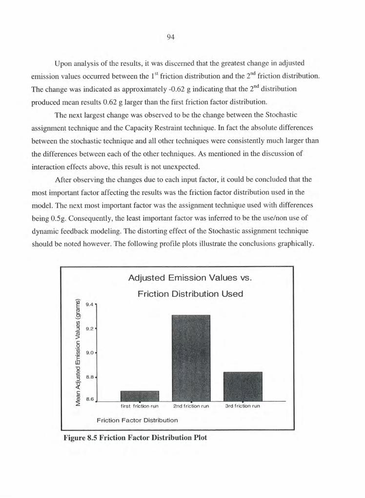
94
Upon analysis of the results, it was discerned that the greatest change in adjusted
emission values occurred between the lst friction distribution and the 2n~ friction distribution,
The change was indicated as approximately -0.62 g indicating that the 2nd distribution
produced mean results 0.62 g larger than the first friction factor distribution.
The next largest change was observed to be the change between the Stochastic
assignment technique and the Capacity Restraint technique. In fact the absolute differences
between the stochastic technique and all other techniques were consistently much larger than
the differences between each of the other techniques. As mentioned in the discussion of
interaction effects above., this result is not unexpected.
After observing the changes due to each input factor, it could be concluded that the
most important factor affecting the results was the friction factor distribution used in the
model, The next most important factor was the assignment technique used with differences
being d.~g. Consequently, the least important factor was inferred to be the use/non use of
dynamic feedback modeling. The distorting effect of the Stochastic assignment technique
should be noted however. The following profile plots illustrate the conclusions graphically.
Adjusted Emission Values vs.
Friction Distribution Used
Mea
n Ad
just
ed E
mis
sion
Val
ues
Gram
s) 9.4
9.2
9.0
8.8
s.s first #riction run 2nd f riction run
Friction Factor Distribution
Figure 8.5 Friction Factor Distribution Plot
3rd f riction run

~~
Mean adj
uste
d Em
issi
on Val
ues (grams)
9.1
9.0
8.9
$.$
Adjusted Errmision~ ~~er~u.s
®ynamic Distribution
_.~~,-ter •3_~'~- ~ . '=
~.T ~ r
no f eedbac k feedback
Feedback/No Feedback
Figure 806 Feedback / No Feedback Plot
~ 9.4
9.3
9.2
O 9.1 .~
9.0
8.9
~_8.8
~ 87
Adjusted Emission Values vs.
Assignment technique
Capacity Restraint Incremental
User Equilibrium
Assignment Technique
Stochastic User Eq u i
Stoc has tic
Figure 8.7 Assignment Technique Plot
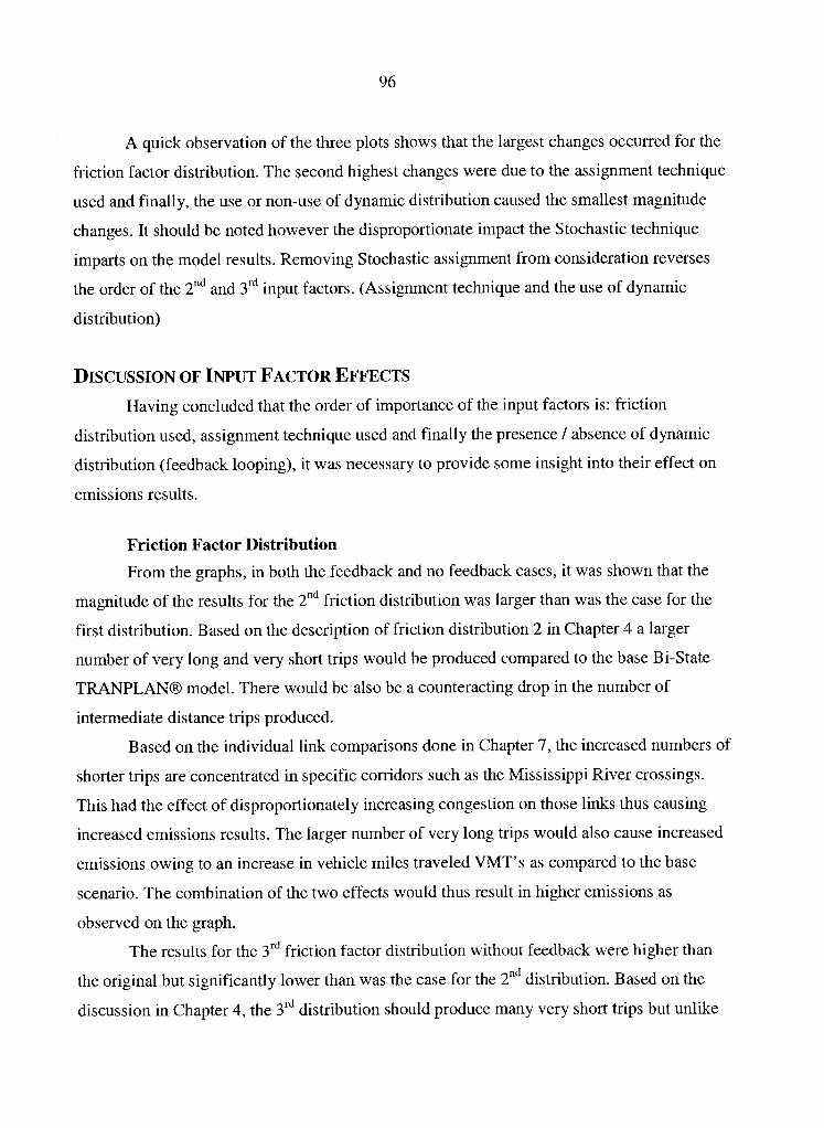
96
A quick observation of the three plots shows that the largest changes occurred for the
friction factor distribution. The second highest changes were due to the assignment technique
used and finally, the use or non-use of dynamic distribution caused the smallest magnitude
changes. It should be noted however the disproportionate impact the Stochastic technique
imparts on the model results. Removing Stochastic assignment from consideration reverses
the order of the 2nd and 3rd input factors. (Assignment technique and the use of dynamic
distribution)
DISCUSSION OF INPUT FACTOR EFFECTS Having concluded that the order of importance of the input factors is: friction
distribution used, assignment technique used and finally the presence I absence of dynamic
distribution (feedback looping), it was necessary to provide some insight into their effect on
emissions results.
Friction Factor Distribution From the graphs, in both the feedback and no feedback cases, it was shown that the
magnitude of the results for the 2nd friction distribution was larger than was the case for the
first distribution. Based on the description of friction distribution 2 in Chapter 4 a larger
number of very long and very short trips would be produced compared to the base B i-State
TRANPLAN® model. There would be also be a counteracting drop in the number of
intermediate distance trips produced.
Based on the individual link comparisons done in Chapter 7, the increased numbers of
shorter trips are concentrated in specific corridors such as the 1Vlississippi River crossings.
This had the effect of disproportionately increasing congestion on those links thus causing
increased emissions results. The larger number of very long trips would also cause increased
emissions owing to an increase in vehicle miles traveled vMT's as compared to the base
scenario. The combination of the two effects would thus result in higher emissions as
observed on the graph.
The results for the 3rd friction factor distribution without feedback were higher than
the original but significantly lower than was the case for the 2nd distribution. Based on the
discussion in Chapter 4, the 3rd distribution should produce many very short trips but unlike

97
the case with the ~nd distribution, there should also be fewer longer trips than was the case in
the original. The fewer number of long trips explain the significantly lower emissions values
than for the 2nd case. Apparently, the greater number of short trips generated enough of an
emissions increase over the base case to counteract the fewer long trips. This resulted in a
moderate increase in emissions over the base case.
When feedbag looping was included, the results for the ~rd distribution were louver
than the case for the original. This is a result of increased predicted emissions in the original
case under feedback looping. In addition, short trips on congested links were most likely
being reassigned to longer but less congested links.
Dynamic Modeling
In general, use of dynamic feedback modeling tended to produce increased emissions.
As stated earlier, the greater travel times in the feedback case increases the proportion of
inefficient vehicle operation due to slower speed, It was also observed that VMTs increased
under dynamic modeling. The net effect of these factors was an increase in emissions values.
Assignment Technique Used
From the graphs, it is apparent that except for the 1 Sz friction distribution used under
the feedback looping scenario, the stochastic assignment technique produced the highest
emissions results of any of the assignment techniques. This is most likely the result of the
Stochastic technique ignoring congestion delay on the greater number of short trips as
described in Chapter 4 for the 2nd and 3~d friction factor distributions. Ignoring congestion
would tend to place vehicles on slower, more congested links as opposed to faster but longer
links. It should be noted that the effect of slower speed {in many cases higher emissions)
operations on links must be .considered in addition to decreased total VMT on shorter links.
The effect on emissions is a complex relationship between type of roadway facility, vehicle
speeds and vehicle miles traveled and in many instances, the effects are counteracting.
The Stochastic User Equilibrium technique produced the next highest emissions
levels. Though this technique has volume delay characteristics, the stochastic probability

98
component influences the result causing increased emissions owing to the same factors
discussed above for the purely Stochastic technique.
The remaining three techniques produced the lowest emissions related to the
assignment technique used. The differences between each of the three were negligible and
could in part be explained by the fact that they all incorporated a similar volume delay
function. In addition, the number of extremely congested (high V/C ratio) links in this model
was small in comparison to other major metropolitan models. This in turn would tend to
minimize the differences between each of the techniques thus explaining the closeness of the
results.
THE EFFECT OF SEASON ON POLLUTANT EMISSIONS
Analysis of aggregate pollutant emissions by season revealed that for all combination
of input factors, emissions were greater in winter than in summer. Table 7.1 in Chapter 7
describes the aggregated emissions by pollutant and season. Illustrated in the following
section are three line graphs displaying the mean emissions change by pollutant for the
winter and summer seasons ignoring all input factors.
Summer ~/s. Winter Mean CO Emissions 160, 000, 000 .~.
~ 140, 000, 000 c~ ~ 120,000,000 ... ~ 100, 000, 000 'N 80, 000, 000 '~ 60, 000, 000 w ~ 40, 000, 000 ca ~ 20, 000, 000
0 1
Summer
Figure 8.8 Mean CO Emissions Difference
2 Wi me r

99
4, 500, 000 .` E 4, 000, 000
... ~ 3, 500, 000 0 .~
'~ 3, 000, 000 uJ
~ 2, 500, 000
2, 000, 000
Summer vs. Winter N+Dx Emissions
1 Summer
2 Winter
Figure 8.9 Mean NOx Emissions Difference
3, 800, 000
3, 600, 000
~ 3, 400, 000
3, 200, 000
® 3, 000, 000 -.~ .~ 2, 800, 000 E ~ 2, 600, 000 -c~ ~ 2, 400, 000 -
2, 200, 000 -
2, 000, 000
Summer vs. Winter N~ Emissions
Summer Winter
Figure X3.10 Mean VOC Emissions Difference

loo
Table 8.7 Percentage Change between Summer and Winter Conditions -- _ - ~ __ , -z
Summer 55,123,918 3,331,237 2,926,127 Winter 145,437,903 4,096,595 3,580,640
%difference 164, 23 22
From the table and graphs, the greatest difference between summer and winter values
was observed for carbon monoxide (CO) emissions. The differences for the other two
pollutants were more moderate being approximately 22% greater. All of the results are best
explained by the tendency of internal combustion engines to burn fuel less efficiently under
very cold conditions. Cold temperatures will inhibit complete combustion of fuel. This
results in a greater proportion of unburnt and incompletely oxidized burnt fuel, hence higher
VOC and CO emissions. The emissions of CO and VOC s in winter are significantly
increased during engine start, warm up and in stop and go traffic. Under these conditions, the
engine does not operate at nol~~ial temperatures; lubricating oil is cold and viscous causing
higher friction and pumping losses and thus increased fuel consumption; and catalytic
converters fail to perform the task of converting the pollutants to carbon dioxide and
atmospheric nitrogen efficiently.
Increased fuel consumption as stated earlier and the specification of the use of a 10°Io
ethanol /gasoline mix in the MOBILE6 emissions factor model are most likely responsible
for the increased NOx winter values. This result is counterintuitive given that NOx is formed
by the oxidation of atmospheric oxygen and nitrogen at high temperatures. Higher fuel
consumption will lead to higher values for all pollutants including NOx.
SUMMARY
In summary, the ANOVA analysis on the inputs indicated that the most significant
input factor was the friction factor distribution used followed by the assignment technique
used with the use or non-use of dynamic modeling being least important. The seasonal
variation in results was indicated in all cases by higher winter emissions than summer
emissions particularly for carbon monoxide with more than a doubling in the values being
noted.

I01
CHAPTER 9. CONCLUSIONS
INPUT FACTOR SIGNIFICANCE AND CONSEQUENCES FOR EMISSIONS
MODELING
As long as transportation is 98°Io dependent on hydrocarbons (petroleum and natural
gas) as fuel sources, (5) automobile emissions will be a matter of concern. Hence, the tools
used to model and forecast future emissions must be clearly understood for proper analyses
to be undertaken. Among the tools used to model future transportation emissions is the 4-step
travel demand model /emissions factor model process. The thesis presented examined the
behavior of this specific forecasting tool with regards to certain input factors and modeling
strategies including the friction factors used, dynamic modeling utilization and the
assignment technique used.
Friction Factor Distribution
The AI~OVA tests and subsequent graphic analysis indicated that the friction
distribution had the greatest effect on the overall model. It was also found that the assignment
technique had a large distorting effect on the model results when the Stochastic assignment
technique was accounted for,
The results indicate that in performing emissions modeling, great care must be taken
when calibrating friction factors. It may be necessary to conduct extensive surveys and
information gathering, some of which were described in Chapter 2 to ensure that the actual
trip performing behavior of the public is accurately captured. Failure to do so may lead to
wildly inaccurate emissions estimates indicating conformitylnon-confor~ility with EPA
emissions regulations than would be the actual case. As is well known by transportation
professionals, the costs of having either situation can be high. For the case where non-
conformity is predicted, federal funding of some transportation infrastructure projects may be
withheld and costly remedial actions undertaken to regain conformity status. For the
converse situation, it must be remembered that the EPA conformity regulations were enacted
primarily to protect the health of the public. Hence, it is likely that the health care costs
would be increased while the physical health of the population diminished potentially leading
to higher mortality rates. Additionally, future emissions monitoring would eventually identify

102
the errors in model predictions. The financial and infrastructure consequences of this
situation can be severe for metropolitan areas.
Dynamic Modeling
It was also made clear from the ANOVA analysis that the use of feedback modeling
had a noticeable emissions effect despite the proportion of high v~C ratio links being
comparatively small. It should be noted however the counteracting factor of peak hour
extrapolation to 24 hours that will tend to minimize the effect of dynamic distribution.
Dynamic feedback modeling is particularly sensitive to high vIC ratios (hence traffic
congestion) in the model for reasons discussed in Chapter 4. This situation clearly illustrates
the disproportionate impact of bottleneck areas in the region such as the bridge crossings and
some freeway links and intersections. With this knowledge, it becomes important to account
for the special effects of bottlenecks in future infrastructure planning. As was the case for the
friction factors, failure to properly plan and account for bottlenecks today could potentially
lead to inappropriate future investments and costly corrective actions.
Assignment Technique
Apart from the Stochastic assignment technique results, the differences between the
techniques used proved that for the Bi-State area emissions modeling, it is not critical that
great emphasis be placed on the assignment technique utilized. Had the All or Nothing
technique been studied as well, similar conclusions could be drawn as those drawn for the
Stochastic assignment approach. Like Stochastic Assignment, the All or Nothing technique
ignores volume delay and would thus have no effect on dynamic modeling.
SEASONAL VARIATIONS
In any emissions modeling scenario, it is important to account for the seasonal
differences in emissions values that can be significant. The environmental and health
concerns are different depending on season. For instance, under winter conditions the main
emissions concern is CO (carbon monoxide) formed by the incomplete combustion of carbon
based fuels. In summer, the main concerns are NOX and VOCs.

~~~
Carbon Monoxide
CO is an emissions concern in winter mainly because of the tendency to have
temperature inversions in winter that make polluted air stay close to ground level, CO
exposure causes detrimental health effects such as nausea, vomiting and if concentrations are
high enough, unconsciousness and even death. Unfortunately, in the very Season for which it
is a primary concern, the predicted CO emissions were observed to be significantly increased
~a factor of approximately 2.~} over the summer values for reasons discussed in Chapter 6.
This implies that careful monitoring and enforcement of regulations limiting CO emissions is
necessary particularly in winter months.
Nitrogen Oxides and Volatile Organic Compounds
Unlike CO, which is primarily a winter emissions problem nitrogen oxides and
volatile organic compounds are summer problems. In addition to specific health problems
related to each pollutant, the two are ingredients in the formation of ozone that is greatest
during hot, bright summer daylight conditions. Fortunately, emissions of VOCs and NOx
were analyzed to be lower in summer months than in winter according to the results from the
MOBILE6 emissions factor model, It must be noted however that specific areas can possibly
register contrasting results depending on local environmental conditions. As with CO in the
winter, it is necessary to carefully control emissions via various strategies. Included among
these strategies are sound future planning arising from emissions modeling, auto
manufacturer regulations, travel demand reduction using transportation control measures,
vehicle emissions testing programs and others.
MODEL APPROACH LIMITATIONS
The research was performed under the following limitations:
1. The derived friction factor curves were not individually calibrated for each
model run. In actual modeling practice, friction factors are painstakingly
calibrated to produce reasonable trip distribution results. Hence, simply changing friction factors without calibration to the model will result in
some error in model predictions.
2. The model assignments were done using the 10% PHF (Peak Hour Factor)
used by the Bi-State Commission and then extrapolated for all hours. This

104
strategy is not ideal as the effect of volume delay is extrapolated beyond the
peak hour when congestion delay will be inconsequential. The result of this
limitation is that recognition must be given to the likelihood that the effect
on the model of dynamic distribution and the assignment technique used
will be over predicted.
3. The sensitivity analysis in this research was performed using future 2025
data that made comparison with ground counts impossible.
4. It is usually more desirable to have the most detailed information feasible.
Included in this information should be a detailed network description
symbolizing the road network at the highest detail possible. Instead of using
a blanket 10°Io peak hour assignment factor for traffic assignment, it would
be preferable to compare assignments hourly against hourly counts from the
B i-State area. This should provide much more relevant information with
regards to emissions modeling. Emissions are highly dependent on the
general traffic conditions with congested periods having disproportionately
higher pollutant emissions .
Correction of these limitations implies that much more data will need to be collected.
Data collection can be an expensive process thus implying that improvements in the
modeling approach described in this thesis will be slow in coming given the differences in
resources between metropolitan areas across the country.
There is also the option to switch to other modeling approaches being introduced such
as the TRANS IMS approach described in Chapter 2. The problem of greater data needs and
processing resources will also slow the adoption of that approach.
FUTURE RESEARCH The traditional four-step travel demand model as its name implies has four stages
with inputs that can be analyzed. The focus of this thesis was on step number 2 and step
number 4, trip distribution and traffic assignment. Future research could extend the
sensitivity analysis to the other two steps.

lay
In trip generation for instance, it would be desirable to determine the emissions effect
of changes in land use patterns, economic conditions and population. These factors all have
significant effects on the trip rates in any particular area. Such studies would help identify the
best patterns of settlement for reduced emissions. (34j it is anticipated that in the near future,
the pattern of settlement will be extensively scrutinized given the projected increases in
automobile traffic. Resources for new infrastructure will become increasing expensive to
procure thus placing great pressure on the efficient use of invested assets. A parallel concern
is the likelihood that transportation energy will become increasingly costly as resource
extraction rates approach a maximum in the near future. This will also place great pressure
on ensuring the most efficient land use and transportation arrangements feasible for a given
area.
An interesting area of future research could involve an investigation into the
.emissions impact of a switch to electric traction and hydrogen fuel in both automobiles and
transit. This would necessitate devising a tool other than MOB ILE6 or similar emissions
factor model that would consider power plant emissions, zero emission electricity sources
and vehicle on board vehicle energy efficiency.
In concluding, the research covered in this thesis has barely scratched the surface of
potential areas for future study as described above. It is hoped that the work initiated here
will be continued as emissions_ and energy concerns become greater.

106
APPENDIX A. FRICTION FACTOR TABLES
Table Al Friction Factors obtained from Bi-State Commission TIME HBW HBQ NHB ~~I TRK
1 10000 10000 10000 10000 10000 2 5248 4467 3548 5248 5432 3 3467 2512 1884 4217 3428 4 2399 1585 1189 2317 2399 5 1778 1059 794 1660 1820 6 1348 794 562 1274 1413 7 1072 631 422 1000 1096 8 871 501 316 794 912 9 724 398 251 638 759 10 602 316 200 525 610 11 501 251 150 347 525 12 416 200 119 363 442 13 355 158 94 302 380 14 302 126 71 260 331 15 263 106 56 219 288 16 224 89 47 188 251 17 195 94 38 160 224 18 170 63 32 138 i97 19 151 53 27 120 168 20 132 47 24 105 150 21 119 40 21 93 135 22 105 38 20 81 122 23 98 33 18 74 110 24 89 30 17 66 10i 25 82 28 16 61 93 26 76 25 16 56 85 27 72 24 16 52 79 28 66 22 15 49 75 29 63 21 15 47 71 30 60 20 15 44 66 31 57 19 15 42 63 32 54 18 14 40 60 33 52 17 14 38 58 34 50 16 13 37 55 35 48 15 13 35 52 36 47 15 13 34 50 37 45 14 13 33 48 38 42 13 13 33 46 39 41 13 13 32 44 40 40 13 13 32 42
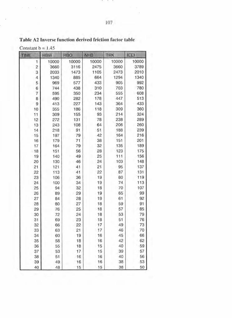
107
Table A2 Inverse function derived friction factor tabie
Constant b = L45 TAME HBW HBQ NHB £~~ TRK lEEi
1 10000 10000 10000 10000 10000 2 3660 3116 2475 3660 3789 3 2033 1473 1105 2473 2010 4 1340 885 664 1294 1340 5 969 577 433 905 992 6 744 438 310 703 780 7 595 350 234 555 608 8 490 282 178 447 513 9 413 227 143 364 433 10 355 186 118 309 360 11 309 155 93 214 324 12 272 131 78 238 289 13 243 108 64 206 260 14 218 91 51 188 239 15 197 79 42 164 216 16 179 71 38 151 201 17 164 79 32 135 189 18 151 56 28 123 175 19 140 49 25 111 156 20 130 46 24 103 148 21 121 41 21 95 137 22 113 41 22 87 131 23 106 36 19 80 119 24 100 34 19 74 113 25 94 32 18 70 107 26 89 29 19 65 99 27 84 28 19 61 92 28 80 27 18 59 91 29 76 25 18 57 85 30 72 24 18 53 79 31 69 23 18 51 76 32 66 22 17 49 73 33 63 21 17 46 70 34 60 19 16 45 66 35 58 18 16 42 62 36 55 18 15 40 59 37 53 17 15 39 57 38 51 16 16 40 56 39 49 16 16 38 53 40 48 i5 15 38 50

108
Table A3 Gamma Function derived friction factor table.
Constant a = 1, b = 1.45, c = 0.025 TIME HBW ~ HBQ ARK ~
__ ~EEI NHB _
2 10000 10000 10000 10000 10000 3 1886 1367 1025 2294 1865 4 1212 801 601 1171 1212 5 855 510 382 799 876 6 641 377 267 605 671 7 500 294 197 466 511 8 401 231 146 366 420 9 330 181 114 291 346 10 276 145 92 241 280 11 235 118 70 163 246 12 202 97 58 176 214 13 175 78 46 149 188 14 154 64 36 132 168 15 135 55 29 113 148 16 120 48 25 101 135 17 107 52 21 88 123 18 96 36 18 78 112 19 87 31 16 69 97 20 79 28 14 63 90 21 72 24 13 56 81 22 65 24 12 50 76 23 60 20 11 45 67 24 55 18 10 41 62 25 50 17 10 37 57 26 46 15 10 34 52 27 43 14 10 31 47 28 40 13 9 29 45 29 37 12 9 27 41 30 34 11 9 25 37 31 32 11 8 23 35 32 30 10 8 22 33 33 28 9 7 20 31 34 26 8 7 19 28 35 24 8 7 18 26 36 23 7 6 16 24 37 21 7 6 15 23 38 20 6 6 16 22 39 19 6 6 15 20 40 17 6 6 14 18

109
APPENDIX B MOBILE6 INPUT FILES (FREEWAY AND ARTERIAL)
Arterial Input File Text MOBILE6 INPUT r II~E DATABASE OUTPUT AGGREGATED OUTPUT WITH FIELDNAIVIES
DATABASE EMISSIONS ; 2222 2222 DATABASE FACILITIES: Arterial DATABASE VEHICLES :22222 22222222 2 222 22222222 222
RUN DATA MINIIVJ~AX TEMP :70.90. SEASON : 1 FUEL RVP : 7.0 OXYGENATED FUELS : 0 .55 0 .035 2
SCENARIO REC :Scenario Title Text -Arterial 2.5 CALENDAR YEAR :2025 AVERAGE SPEED : 2.5 Arterial EVALUATION MONTH : 7
SCENARIO REC :Scenario Title Text -Arterial 5 CALENDAR YEAR :2025 AVERAGE SPEED : 5 Arterial EVALUATION MONTH : 7
SCENARIO REC :Scenario Title Text -Arterial 10 CALENDAR YEAR :2025 AVERAGE SPEED : 10 Arterial EVALUATION MONTH : 7
SCENARIO REC :Scenario Title Text -Arterial 15 CALENDAR YEAR :2025 AVERAGE SPEED : 15 Arterial EVALUATION MONTH : 7
SCENARIO REC :Scenario Title Text -Arterial 20 CALENDAR YEAR :2025 AVERAGE SPEED : 20 Arterial EVALUATION MONTH : ~
SCENARIO REC :Scenario Title Text -Arterial 25 CALENDAR YEAR :2025

X10
AVERAGE SPEED - : 25 Arterial EVALUATION MONTH ; 7
SCENARIO REC :Scenario Title Text - Arteria130 CALENDAR YEAR :2025 AVERAGE SPEED : 30 Arterial EVALUATION MON'T'H : 7
SCENARIO REC :Scenario Title Text -Arterial 35 CALENDAR YEAR :2025 AVERAGE SPEED : 35 Arterial EVALUATION MONTH : 7
SCENARIO REC :Scenario Title Text - Arteria140 CALENDAR YEAR :2025 AVERAGE SPEED : 40 Arterial EVALUATION MONTH : 7
SCENARIO REC :Scenario Title Text - Arteria145 CALENDAR YEAR :2025 AVERAGE SPEED : 45 Arterial EVALUATION MONTH : 7
SCENARIO REC :Scenario Title Text - Arteria150 CALENDAR YEAR :2025 AVERAGE SPEED : 50 Arterial EVALUATION MONTH : 7
SCENARIO REC :Scenario Title Text -Arterial 55 CALENDAR YEAR :2025 AVERAGE SPEED : 55 Arterial EVALUATION MONTH : 7
SCENARIO REC :Scenario Title Text - Arteria160 CALENDAR YEAR :2025 AVERAGE SPEED : 60 Arterial EVALUATION MONTH : 7
SCENARIO REC :Scenario Title Text - Arteria165 CALENDAR YEAR :2025 AVERAGE SPEED : 65 Arterial EVALUATION MONTH : ~
END OF RUN
MINIIVl~AX TEMP : 10.20. SEASON : 2 ~~ I~EL RVP : 7.0 OXYGENATED BLS : 0 .55 0 .035 2

~1~
SCENARIO REC :Scenario Title 'Text -Arterial 2.5 CALENDAR YEAR :2025 AVERAGE SPEED : 2.5 Arterial
SCENARIO REC :Scenario Title Text -Arterial 5 CALENDAR YEAR :2025 AVERAGE SPEED : 5 Arterial
SCENARIO REC :Scenario Title Text -Arterial 10 CALENDAR YEAR :2025 AVERAGE SPEED : 10 Arterial
SCENARIO REC :Scenario 'Title Text -Arterial 15 CALENDAR YEAR :2025 AVERAGE SPEED : 15 Arterial
SCENARIO REC :Scenario Title Text -Arterial 20 CALENDAR YEAR :2025 AVERAGE SPEED : 20 Arterial
SCENARIO REC :Scenario Title Text -Arterial 25 CALENDAR YEAR :2025 AVERAGE SPEED : 25 Arterial
SCENARIO REC :Scenario Title Text -Arterial 30 CALENDAR YEAR :2025 AVERAGE SPEED : 30 Arterial
SCENARIO REC :Scenario Title Text -Arterial 35 CALENDAR YEAR :2025 AVERAGE SPEED : 35 Arterial.
SCENARIO REC :Scenario Title Text -Arterial 40 CALENDAR YEAR :2025 AVERAGE SPEED : 40 Arterial
SCENARIO REC :Scenario Title Text - Arteria145 CALENDAR YEAR :2025 AVERAGE SPEED : 45 Arterial

112
SCENARIO REC :Scenario Title Text -Arterial 50 CALENDAR YEAR :2025 AVERAGE SPEED : SO Arterial
SCENARIO REC :Scenario Title Text -Arterial 55 CALENDAR YEAR :2025 AVERAGE SPEED : 55 Arterial
SCENARIO REC :Scenario Title Text -Arterial 60 CALENDAR YEAR :2025 AVERAGE SPEED : 60 Arterial.
SCENARIO REC :Scenario Title Text -Arterial 65 CALENDAR YEAR :2025 AVERAGE SPEED : 65 Arterial
END OF RUN
Figure B 1 Arterial Input File
Freeway Input File Text MOBILE6 INPUT N~L,E DATABASE OUTPUT AGGREGATED OUTPUT WITH F~LDNAII~S
DATABASE EMISSIONS :2222 2222 DATABASE FACILITIES: Freeway DATABASE VEHICLES :22222 22222222 2 222 22222222 222
RUN DATA MINI~VIAX TEMP :70.90. SEASON : 1 FUEL RVP : 7.0 OXYGENATED FUELS 0 .55 0 .035 2
SCENARIO REC :Scenario Title Text -Freeway 2.5 CALENDAR YEAR :2025 AVERAGE SPEED : 2.5 Freeway EVALUATION MONTH : 7
SCENARIO REC :Scenario Title Text -Freeway 5 CALENDAR YEAR :2025

113
AVERAGE SPEED : 5 Freeway EVALUATION MONTH : 7
SCENARIO REC :Scenario Title Text -Freeway l0 CALENDAR YEAR :2025 AVERAGE SPEED : l0 Freeway EVALUATION MONTH : 7
SCENARIO REC :Scenario Title Text -Freeway 15 CALENDAR YEAR :2025 AVERAGE SPEED : 15 Freeway EVALUATION MONTH : 7
SCENARIO REC :Scenario Title Text -Freeway 20 CALENDAR YEAR :2025 AVERAGE SPEED : 20 Freeway EVALUATION MONTH : 7
SCENARIO REC :Scenario Title Text -Freeway 25 CALENDAR YEAR :2025 AVERAGE SPEED : 25 Freeway EVALUATION MONTH : 7
SCENARIO REC :Scenario Title Text -Freeway 30 CALENDAR YEAR :2025 AVERAGE SPEED : 30 Freeway EVALUATION MONTH : 7
SCENARIO REC :Scenario Title Text -Freeway 35 CALENDAR YEAR :2025 AVERAGE SPEED : 35 Freeway EVALUATION MONTH : 7
SCENARIO REC :Scenario Title Text -Freeway 40 CALENDAR YEAR :2025 AVERAGE SPEED : 40 Freeway EVALUATION MONTH : 7
SCENARIO REC :Scenario Title Text -Freeway 45 CALENDAR YEAR :2025 AVERAGE SPEED : 45 Freeway EVALUATION MONTH : 7
SCENARIO REC :Scenario Title Text -Freeway 50 CALENDAR YEAR :2025 AVERAGE SPEED : 50 Freeway EVALUATION MONTH : 7
SCENARIO REC :Scenario Title Text -Freeway 55

114
CALENDAR YEAR :2025 AVERAGE SPEED : SS Freeway EVALUATION MONTH : 7
SCENARIO REC :Scenario Title Text -Freeway 60 CALENDAR YEAR :2025 AVERAGE SPEED : 60 Freeway EVALUATION MONTH : 7
SCENARIO REC :Scenario Title Text -Freeway 65 CALENDAR YEAR :2025 AVERAGE SPEED : 6S Freeway EVALUATION MONTH : 7
END OF RUN
1VIIN/~VJ[AX TEMP : 10. 20. SEASON : 2 FUEL RVP : 7.0 OXYGENATED FUELS : 0 O.SS 0 0.035 2
SCENARIO REC :Scenario Title Text -Freeway 2.S CALENDAR YEAR :2025 AVERAGE SPEED : 2.5 Freeway
SCENARIO REC :Scenario Title Text -Freeway S CALENDAR YEAR :2025 AVERAGE SPEED : S Freeway
SCENARIO REC :Scenario Title Text -Freeway 10 CALENDAR YEAR :2025 AVERAGE SPEED : 10 Freeway
SCENARIO REC :Scenario Title Text -Freeway 1 S CALENDAR YEAR :2025 AVERAGE SPEED : 1 S Freeway
SCENARIO REC :Scenario Title Text -Freeway 20 CALENDAR YEAR :2025 AVERAGE SPEED : 20 Freeway
SCENARIO REC :Scenario Title Text -Freeway 25 CALENDAR YEAR :2025 AVERAGE SPEED : 25 Freeway

115
SCENARIO REC .CALENDAR YEAR AVERAGE SPEED
SCENARIO REC : CALENDAR YEAR AVERAGE SPEED
SCENARIO REC : CALENDAR YEAR AVERAGE SPEED
SCENARIO REC CALENDAR YEAR AVERAGE SPEED
SCENARIO REC CALENDAR YEAR AVERAGE SPEED
SCENARIO REC CALENDAR YEAR AVERAGE SPEED
SCENARIO REC CALENDAR YEAR AVERAGE SPEED
SCENARIO REC CALENDAR YEAR AVERAGE SPEED
END OF RUN
Scenario Title Text -Freeway 30 2025
30 Freeway
Scenario Title Text -Freeway 35 2025
35 Freeway
Scenario Title 'Text -Freeway 40 2025
40 Freeway
Scenario Title Text -Freeway 45 2025
45 Freeway
Scenario Title Text -Freeway 50 : 2025 50 Freeway
Scenario Title Text -Freeway 55 2025
55 Freeway
Scenario Title Text -Freeway b0 2025
60 Freeway
Scenario Title Text -Freeway 65 2025
65 Freeway
Figure B2 Freeway Input File

116
APPENDIX C VISUAL BASIC CODE AND PROGRAM SCREENSHOT
■ Combine
c:
c: ~ modelling
~ frickianscenarial r.~~~.~r:It!,~
,~ feedback .,,~ regular
capflow~2. bin ca • flo~2. dcb i=iJr~:1E~ C.~2.DBF COMB_CAP.DBF CO ~ B_CAP. ~ D combined. mtx cambinedl .mkx distributian.mkx distributionl.mkx FE E D BACK. D B F origdest. mkx origdestl .mkx shortest. mkx shartestl .mkx
_~o
Figure C1 Screenshot of Program Used to Combine the Travel Demand Model Results with MOBILE6 Results

~~~
11~iain Form Code
Private mPath As String Private Sub Form_Load{)
istDiriist.Path =1stDrive.Drive & "1"
End Sub
Private Sub Form_IJnload{Cancel As Integer)
Set mDBEngine =Nothing Set bldTable =Nothing Set clsrun =Nothing Set mdatabase ~ =Nothing Set mrecordset 1 =Nothing Set mSummerfreeway.= Nothing Set mSummerfreewayl =Nothing Set mSummerfreeway2 =Nothing Set mwinterfreeway =Nothing Set mwinterfreeway l =Nothing Set mwinterfreeway2 =Nothing
End Sub
Private Sub 1stDirlist_Change{)
1stFiie.Path =1stDirlist.Path
End Sub
Private Sub 1stDirlist_Click{)
1stFile.Path =1stDirlist.Path
End Sub
Private Sub 1stDrive_Change{)
1stFile.Path = istDrive.Drive 1stDirlist.Path =1stDrive.Drive
End Sub
Private Sub istFiie_DblClick{} Dim mDBEngine As New DAO.DBEngine Dim mdatabase As DAO.Database Dim mrecordset 1 As DAO.Recordset Dim mSummerfreeway As Collection Dim mSummerfreeway2 As Collection Dim mSummerfreeway~ As Collection Dim mwinterfreeway As Collection Dim mwinterfreeway2 As Collection Dim mwinterfreeway3 As Collection

118
Dim mSummerarterial. As Collection Dim mSummerarterial2 As Collection Dim mSummerarterial3 As Collection Dim mWinterarterial As Collection Dim mwinterarterial2 As Collection Dim mWinterarterial3 As Collection Dim init seen As Integer Dim agg_break As Boolean Dim clsrun As clsPerformrun Dim bldTable As c1sDBbuilder Dim wieghted_pol As Double
mPath = App.Path Set bldTable =New c1sDBbuilder bldTable.prgPath =1stFile.Path bldTable.maketable Set mdatabase = mDBEngine.OpenDatabase{mPath, False, False, "DBASE N" )
' Hydrocarbon emissions Summer Set mrecordsetl = mdatabase.~penRecordset("select *from freeway where run = 1 and pol = 1") mrecordset 1.MoveFirst init_scen = mrecordsetl.Fields{"scen").value Set mSummerfreeway =New Collection weighted_pol = 0 Do While Not mrecordset l .EOF
If init_scen <> mrecordset 1.Fields{"scen" ).value Then init_scen = mrecordset l .Fields{"scen" ).value mSummerfreeway.Add weighted_pol weighted_pol = 0
End If weighted_pol = weighted_pol + mrecordset 1.Fields{" gm_mile" ).value * mrecordset l .Fields{" vmt" ) mrecordset 1.MoveNext
Loop
mSummerfreeway.Add weighted_pol Set rnrecordset 1 =Nothing
' CO emissions Summer Set mrecordsetl = mdatabase.~penRecordset("select *from freeway where run = 1 and pol = 2") mrecordset 1.MoveFirst init_scen = mrecordsetl.Fields{"scen").value Set mSummerfreeway2 =New Collection weighted_pol = 0 Do While Not mrecordset 1.EC~F
if init_scen <> mrecordset l .Fields{"scen" ).value Then init_scen = mrecordset 1.Fields{"scen" ). value mSummerfreeway2.Add weighted_pol weighted_pol = 0
End If weighted_pol = weighted_poI + mrecordset l .Fields{" gm_mile" }.value * mrecordset 1.Fields{" vmt" ) mrecordset 1.MoveNext
Loop mSummerfreeway2.Add weighted_pol Set mrecordset 1 =Nothing

119
' NOX emissions Summer Set mrecordset 1 = mdatabase.OpenRecordset("select *from freeway where run = 1 and pol = 3" ) mrecordset l .1VIoveFirst -init_scen = mrecordset i .Fields{" seen" ).value Set mSummerfree~vay3 =New Collection we ighted_po 1= 0 Do While Not mrecordset 1.EOF
If init_scen <> mrecordset 1.Fields("seen" ).value Then init seen = mrecordset l .Fields("seen" ).value mSummerfreeway3.Add weighted pol weighted_pol = 0
End If weighted_pol = weighted_pol + mrecordset l .Fields{"gm_mile" ).value ~ mrecordset l .Fields(" vmt" ) mrecordset l .1VIoveNext
Loop mSummerfreeway3.Add weighted_pol Set mrecordset 1 =Nothing
' Hydrocarbon emissions Winter Set mrecordset 1 = mdatabase.OpenRecordset("select *from freeway where run = 2 and pol = 1") mrecordset l .1VIoveFirst init seen = mrecordsetl.Fields("seen").value Set mWinterfreeway =New Collection weighted_pol = 0 Do While Not mrecordset i .EOF
If init seen <> mrecordset l .Fields("seen").value Then init_scen = mrecordset l .Fields(" seen" ).value mWinterfreeway.Add weighted_pol weighted_pol = 0
End If weighted_pol = weighted_pol + mrecordset 1.Fields{" gm_miie" ).value * mrecordset 1.Fields(" vmt" ) mrecordset l .MoveNext
Loop mWinterfreeway.Add weighted_pol Set mrecordset 1 =Nothing
' CO emissions Winter Set mrecordset 1 = mdatabase.OpenRecordset("select *from freeway where run = 2 and pol = 2" ) mrecordset l .1VIoveFirst init seen = mrecordset 1.Fieids("seen" ).value Set mWinterfreeway2 =New Collection weighted_pol = 0 Do While Not mrecordset l .EOF
If init_scen <> mrecordset 1.Fields("seen" ).value Then init seen = mrecordset 1.Fields("seen" ).value mWinterfreeway2.Add weighted_pol weighted_pol = 0
End If weighted_pol = weighted_pol + mrecordset l .Fields("gm_mile" ).value * mrecordset l .Fields(" vmt" ) mrecordset l .MoveNext
Loop mWinterfreeway2.Add weighted_pol Set mrecordset l =Nothing

12O
' NOX emissions winter Set mrecordset 1 = mdatabase.OpenRecordset{"select *from freeway where run = 2 and pol = 3") mrecordset 1.MoveFirst init scen = mrecordset l .Fields{"scen" ).value Set mWinterfreeway3 =New Collection weighted_pol = 0 Do While Not mrecordset l .EOF
if init_scen <> mrecordset l .Fields("scen" ).value Then init_scen = mrecordsetl.Fields("scen").value mWinterfreeway3.Add weighted_pol weighted_pol = 0
End If weighted_pol = weighted_pol + mrecordset l .Fields{" gm_mile" ).value * mrecordset l .Fields{" vmt" ) mrecordset l .MoveNext
Loop mWinterfreeway3.Add weighted_pol Set mrecordset 1 =Nothing
' Arterial ' Hydrocarbon emissions Summer
Set mrecordset 1 = mdatabase.OpenRecordset("select *from arterial where run = 1 and pol = 1 ") mrecordset 1.MoveFirst init_scen = mrecordset l .Fields(" scen" ).value Set mSummerarteriai =New Collection weighted_pol = 0 Do While Not mrecordset i .EOF
if init_scen <> mrecordset l .Fields{"scen") .value Then init_scen = mrecordsetl.Fields("scen").value mSummerarterial.Add weighted_pol weighted pol = 0
End If weighted_pol = weighted_pol + mrecordset i .Fields(" gm_mile" ).value * mrecordset l .Fields(" vmt" ) mrecordset l .MoveNext
Loop mSummerarterial.Add weighted_pol Set mrecordset 1 =Nothing
' CO emissions Summer Set mrecordset 1 = mdatabase.OpenRecordset("select *from Arterial where run = 1 and poi = 2" ) mrecordset l .MoveFirst init scen = mrecordset l .Fields{"scen" ).value Set mSummerarterial2 =New Collection weighted_pol = 0 Do While Not mrecordset l .EOF
If init_scen <> mrecordset l .Fields(" scen" ).value Then init_scen = mrecordset l .Fields(" scen" ).value mSummerarterial2.Add weighted_pol weighted_pol = 0
End If weighted_pol = weighted_pol + mrecordset 1.Fields(" gm_mile" ).value * mrecordset l .Fields("vmt" ) mrecordset l .1VIoveNext
Loop

121
mSummerarterial2.Add weighted_pol Set mrecordset 1 =Nothing
' NOS emissions Summer Set mrecordset 1 = mdatabase.OpenRecordset{"select *from Arterial where run = 1 and poi = 3") mrecordset l .MoveFirst init_scen = mrecordset l .Fields{"scen" ).value Set mSummerarterial3 =New Collection weighted_pol = 0 Do While Not mrecordset 1.EOF
If init scen <> mrecordsetl.Fieids("scen"}.value Then init scen = mrecordset l .Fields(" scen" ).value mSummerarteriai3.Add weighted_pol weighted_po1= 0
End If weighted_pol = weighted poi + mrecordset l .Fields("gm_miie" }.value * mrecordset i .Fields("vmt" ) mrecordset 1.MoveNext
Loop mSummerarteriai3.Add weighted_pol Set mrecordset l =Nothing
' Hydrocarbon emissions Winter Set mrecordset 1 = mdatabase.OpenRecordset("select *from Arterial where run = 2 and poi = 1 ") mrec o rd s e t t. Mo veFir s t init_scen = mrecordset l .Fields{"scen" ).value Set mWinterarterial =New Collection weighted_po1= 0 Do While Not mrecordset l .EOF
If init_scen <> mrecordset l .Fields(" scen" ).value Then init scen = mrecordset I .Fields{"scen" ).value mWinterarterial.Add weighted_poi weighted_pol = 0
End if weighted_poi = weighted_pol + mrecordset l .Fields{" gm_mile" }.value * mrecordset l .Fields{"vmt" ) mrecordset l .MoveNext
Loop mWinterarterial.Add weighted_pol Set mrecordset 1 =Nothing
' CO emissions Winter Set mrecordsetl = mdatabase.OpenRecordset{"select *from Arterial where run = 2 and pol = 2") mrecordset l .MoveFirst init_scen = mrecordset i .Fields("scen" ).value Set mWinterarterial2 =New Collection weighted_pol = 0 Do While Not mrecordset l .EOF
If init scen <> mrecordset i ..Fields("scen" ).value Then init scen = mrecordset l .Fields{"scen" ).value mWinterarterial2.Add weighted poi weighted_poi = 0
End If weighted_pol = weighted_pol + mrecordset l .Fields(" gm_mile" ).value * mrecordset l .Fields("vmt" ) mrecordset I .Movel~Text
Loop
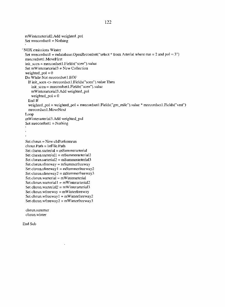
122
mWinterarterial2.Add weighted_pol Set mrecordset 1 =Nothing
' NOX emissions Winter Set mrecordsetl = mdatabase.OpenRecordset("select *from Arterial where run = 2 and pol = 3") mrecordset l .MoveFirst init_scen = mrecordset l .Fields(" scen" ).value Set mWinterarterial3 =New Collection weighted_pol = 0 Do While Not mrecordset l .EOF
If init_scen <> mrecordset l .Fields(" scen") .value Then init scen = mrecordsetl.Fields("scen").value mWinterarterial3.Add weighted_pol weighted_pol = 0
End If weighted_pol = weighted_pol + mrecordset l .Fields(" gm_mile" ).value * mrecordset l .Fields(" vmt" ) mrecordset l .MoveNext
Loop mWinterarterial3.Add weighted_pol Set mrecordset 1 =Nothing
Set clsrun = New clsPerformrun cisrun.Path =1stFile.Path Set clsrun.sarterial = mSummerarterial Set clsrun.sarteriai i = mSummerarterial2 Set clsrun.sarterial2 = mSummerarterial3 Set clsrun.sfreeway = mSummerfreeway Set clsrun.sfreeway 1 = mSummerfreeway2 Set clsrun.sfreeway2 = mSummerfreeway3 Set clsrun. warterial = mWinterarterial Set clsrun. warterial 1 = mWinterarterial2 Set clsrun.warterial2 = mWinterarterial3 Set clsrun.wfreeway = mWinterfreeway Set clsrun. wfreeway 1 = mW interfreeway2 Set clsrun.wfreeway2 = mWinterfreeway3
clsrun.summer clsrun. winter
End Sub

l~~
Summer and V~inter Processing Code
Private mSfreeway As Collection Private mSfreeway ~ As Collection Private mSfreeway2 As Collection Private mV~freeway As Collection Private mWfreeway 1 As Collection Private mWfreeway2 As Collection Private mSarterial As Collection. Private m5arteriall As Collection Private mSarterial2 As Collection Private mwarterial As Collection Private mWarterial ~ As Collection Private mWarterial2 As Collection Private mDBEngine As New DAO.DBEngine Private mdatabase As DAO.Database Private mRecordset As DAO.Recordset Private SNOX recset As DAO.Recordset Private SCO recset As DAO.Recordset Private SVOC recset As DAO.Recordset Private WNOX recset As DAO.Recordset Private WCO recset As DAO.Recordset Private WVOC recset As DAO.Recordset Private mPath As String Private filename As String Private total emission he As Double Private total emission co As Double Private total emission nox As Double
Public Property Let Path{ByVal value As String)
mPath =value filename = Left(Forml.lstFi~e.FileName, 8) Set mdatabase = mDBEngine.OpenDatabase(mPath, False, False, "DBASE IV") Set mRecordset = mdatabase.OpenRecordset("select *from " & filename)
End Property
Public Property Set sfreeway(ByVai value As Variant)
Set mSfreeway =value
End Property
Public Property Set sfreeway 1 {ByVal value As Variant)
Set mSfreeway 1 =value
End Property
Public Property Set sfreeway2{ByVal value As Variant)
Set mSfreeway2 =value

~~
End Property
Public Property Set wfreeway(ByVal value As Variant)
Set mVVfreeway =value
End Property
Public Property Set wfreeway 1{ByVal value As Variant)
Set mwfreeway l =value
End Property
Public Property Set wfreeway2(ByVal value~As Variant)
Set mwfreeway2 =value
End Property
Public Property Set sarterial(ByVal value As Variant)
Set mSarterial =value
End Property
Public Property Set sarterial 1(ByVal value As Variant)
Set mSarteriall =value
End Property
Public Property Set sarterial2{ByVal value As Variant)
Set mSarterial2 =value
End Property
Public Property Set warterial(ByVal value As Variant}
Set mwarterial =value
End Property
Public Property Set warterial 1(ByVal value As Variant)
Set mwarterial) =value
End Property
Public Property Set warterial2(ByVai value As Variant)
Set rnwarterial2 =value

125
End Property
Public Sub summer{) Dim speed As Double Dim scenario As Integer
Set SNOX_recset = mdatabase.OpenRecordset("select *from SNOX_com") Set SVOC_recset = mdatabase.OpenRecordset{"select *from SVOC_com" ) Set SCO_recset = mdatabase.OpenRecordset{"select *from SCO_comb")
mRecordset.MoveFirst
Do While Not mRecordset.EOF SNOX recset.AddNew SVOC recset.AddNew SCO_recset.AddNew If mRecordset.Fields{"BA_SPEED") <> Null Then
speed = mRecordset.Fields{"AB_SPEED") + mRecordset.Fields{" BA_SPEED" )12 Else
speed = mRecordset.Fields{" AB_SPEED" ) End If
Select Case speed Case 0 To 2.5
scenario = 1. Case 2.5 i To 5
scenario = 2 Case 5.1 To 10
scenario = 3 Case 10.1 To 15
scenario = 4 Case 15.1 To 20
scenario = 5 Case 20.1 To 25
scenario = 6 Case 25.1 To 30
scenario = 7 Case 30.1 To 35
scenario = 8 Case 35. i To 40
scenario = 9 Case 40.1 To 45
scenario = 10 Case 45.1 To 50
scenario = 11 Case 50.1 To 55
scenario = 12 Case 55.1 To b0
scenario = 13 Case b0. l To b5
scenario = 14 End Select
If mRecordset.Fields{"group_code").value = 1 Or mRecordset.Fields{"group_code").value = 2 Then

126
totai_emiss~on_hc = mSfreeway.Item(scenario) * mRecordset.Fields{"length").value * _ mRecordset.Fields{"tot_flo w" ).value
summer_add~.fields "hc", total_emission he total_emission co = mSfreewayl.Item{scenario) * mRecordset.Fields{"length").value * _
mRecordset.Fields{"tot_flow" ). value summer add fields "co", total_emission co total_emission nox = mSfreeway2.Item(scenario) * mRecordset.Fields{"length").value * _
mRecordset.Fieids{" tot flow" ).value summer_add_fields "nox", total_emissionnox
ElseIf mRecordset.Fields{" group code" ).value > 2 Then total emission he = mSarterial.Item{scenario) * mRecordset.Fields{"length").value * _
mRecordset.Fields{"tot flow").value summer_add_fields "hc", total emission he total_emission_co = mSarteriall.Item{scenario) * mRecordset.Fields{"length").value * _
mRecordset.Fieids{"tot_flow" ).value summer add ~ieids "co", total_emission_co total_emission_nox = mSarteriai2.Item(scenario) * mRecordset.Fields{"length").value * _
mRecordset.Fieids{" tot_flow" ).value summer_add_fields "nox", totai_emission_nox
End If
SNOX_recset.Update SVOC_recset.Update SCO_recset.Update mRecordset.MoveNext
Loop
Set SNOX_recset =Nothing Set SVOC_recset =Nothing Set SCO_recset =Nothing
End Sub
Public Sub winter{) Dim speed As Double Dim scenario As Integer
Set WNOX_recset = mdatabase.OpenRecordset{"select *from WNOX_com") Set WVOC_recset = mdatabase.OpenRecordset{"select *from WVOC_com" ) Set WCO_recset = mdatabase.OpenRecordset{"select *from WCO_comb" )
mRecordset. Mo veFirst
Do While Not mRecordset.EOF WNOX_recset.AddNew WVOC_recset.AddNew WCO_recset.AddNew
If mRecordset.Fieids("BA_SPEED") <> Nuil Then speed = mRecordset.Fields("AB_SPEED") + rnRecordset.Fields("BA_SPEED") / 2
Else speed = mRecordset.Fields{"AB_SPEED" )
End If

~2~
Select Case speed Case 0 To 2.5
scenario = 1 Case 2.51 To 5
scenario = 2 Case 5.1 To 10
scenario = 3 Case 10,1 To 15
scenario = 4 Case 15.1 To 20
scenario = 5 Case 20.1 To 25
scenario = 6 Case 25.1 To 30
scenario = 7 Case 30.1 To 35
scenario = 8 Case 35.1 To 40
scenario = 9 Case 40.1 To 45
scenario = 10 Case 45.1 To 50
scenario = 11 Case 50.1 To 55
scenario = 12 Case 55.1 To 60
scenario = 13 Case 60.1 To 65
scenario = 14 End Select
If mRecordset.Fields("group code").value = 1 Or mRecordset.Fields("group_code").value = 2 Then total_emission_hc = mWfreeway.Item{scenario) * mRecordset.Fieids("length").value * _
mRecordset.Fields{"tot flow").value winter_add_fields "hc", total_emission_hc total emission co = mWfreewayl.Item{scenario) *mRecordset.Fields("length").value * _
mRecordset.Fields{" tot_flow" ).value winter_add_fields "co", total emission co total_ernission nox. = mWfreeway2.Item(scenario) * mRecordset.Fieids("length").value * _
mRecordset.Fields{"tot_flow" ).value winter_add_fieids "nox", total_emission_nox
ElseIf mRecordset.Fields("group code").value > 2 Then total_emissionhc = mWarterial.Item(scenario) *mRecordset.Fields("length").value * _
mRecordset.Fields{"tot_flow").value winter_add_fields "hc", totai_emission_hc totatemission_co = mWarteriall.Item(scenario) *mRecordset.Fields{"length").value * _
mReco rds et. Field s {" to t_flo w") .value winter_add_fields "co", totai_emission_co total emission nox = mWarterial2.Item(scenario) * mRecordset.Fields~"length").value * _
mRecordset.Fields{" tot_flo w" ).value winter_add_fieids "nox", total_emission_nox
End If
WNOX_recset.Update

128
WVOC_recset.Update WCO_recset.Update mRecordset.MoveNext
Loop
Set WNOX_recset =Nothing Set WVOC_recset =Nothing Set WCO_recset =Nothing
End Sub
Private Sub summer_add_fields{emm type As String, emissions As Double)
If emm_type = "hc" Then cnt=0 Do While cnt < SVOC recset.Fields.Count - 1
SVOC_recset.Fields{cnt).value = mRecordset.Fields{cnt).value cnt=cnt+ 1
Loop SVOC_recset,Fields{cnt).value =emissions
ElseIf emm_type = "co" Then cnt=0 Do While cnt < SCO recset.Fields.Count - 1
SCO_recset.Fields(cnt).value = mRecordset.Fields(cnt).value cnt=cnt+l
Loop SCO_recset.Fields{cnt).value =emissions
ElseIf emm_type = "nox" Then cnt=0 Do While cnt < SNOX recset.Fields.Count - 1
SNOX_recset.Fields{cnt).value = mRecordset.Fields{cnt).value cnt=cnt+1
Loop SNOX_recset.Fields{cnt).value =emissions
End If
End Sub
Private Sub winter_add_fields{emm_type As String, emissions As Double)
if emm_type = "hc" Then cnt = 0 Do While cnt < WVOC recset.Fields.Count - 1
WVOC_recset.Fields{cnt).value = mRecordset.Fields{cnt).value cnt=cnt+l
Loop WVOC_recset.Fields{cnt).value =emissions
ElseIf emm type = "co" Then cnt=0 Do While cnt < WCO recset.Fields.Count - 1
WCO_recset.Fields{cnt).value = mRecordset.Fields(cnt).value cnt=cnt+1
Loop WCO_recset.Fields{cnt}.value =emissions

129
ElseIf emm type = "nox" Then cnt=0 Do While cnt < WNOX recset.Fields.Count - 1
WNOX_recset.Fields(cnt).value = mRecordset.Fields{cnt).value cnt=cnt+l
Loop WNOX_recset.Fields{cnt).value =emissions
End If
End Sub
Private Sub Class_Terminate{)
Set mdatabase =Nothing Set mRecordset =Nothing Set mDBEngine =Nothing
End Sub

~ 30
Fide 11~Ianipula~ion Code
Option Explicit
Private mEmissions As Double Private mPath As String Private mDBE As New DAO.DBEngine Private mOutputdatabase As DAO.Database
Public Property Let prgPath{ByVal value As String)
mPath =value
End Property
Public Sub maketable() Dim mNewdef ~ As TableDef Dim mNewdef2 As TableDef Dim mNewdef3 As TableDef Dim mNewdef4 As TableDef Dim mNewdef5 As TableDef Dim mNewdefC As TableDef Dim mFieid As Field Dim cnt As Integer Dim filename As String
On Error GoTo delete file
Set mOutputdatabase = mDBE.OpenDatabase(mPath, False, False, "DBASE IV;") Set mNewdef 1 =New TableDef Set mNewdef2 =New TableDef Set mNewdef3 =New TableDef Set mNewdef4 =New TableDef Set mNewdefS =New TableDef Set mNewdef6 =New TableDef
filename =Left{Forml.lstFile.FileName, S) mNewdef l .Name = "SNOX_" & mOutputdatabase.TableDefs(file_name).Name mNewdef2.Name = "SCO_" & mOutputdatabase.TableDefs(file_name).Name mNewdef3.Name = "SVOC_" & mOutputdatabase.TableDefs(file_name).Name mNewdef4.Name = "WNOX_" & mOutputdatabase.TableDefs(file_name).Name mNewdefS.Name = "WCO_" & mOutputdatabase.TableDefs{fiie_name).Name mNewdef6.Name = "WVOC_" & mOutputdatabase.TableDefs(file_name),Name
cnt=0 Do While cnt < mOutputdatabase.TableDefs{file_name).Fields.Count
Append mNewdef 1, cnt, filename Append mNewdef2, cnt, filename Append mNewdef3, cnt, filename Append mNewdef4, cnt, filename Append mNewdef5, cnt, filename Append mNewdefb, cnt, filename cnt=cnt+l

131
Loop
Set mField =New Field Appendend mNewdef 1 Appendend mNewdef2 Appendend mNewdef3 Appendend mNewdef4 Appendend r~~Newdef5 Appendend mNewdefb
s
mDutputdatabase.TableDefs m0 utp utdatabase. TableDefs m0utputdatabase.TableDefs mOutp utdatabase.TableDefs mOutp utdatabase.TableDefs mOutputdatabase.TableDefs
.Append mNewdef 1
.Append mNewdef2
.Append mNewdef3
.Append mNewdef4
.Append mNewdef5
.Append mNewdefb
Set mDBE =Nothing Set mOutputdatabase =Nothing Set mNewdef l =Nothing Set mNewdef2 =Nothing Set mNewdef3 =Nothing Set mNewdef4 =Nothing Set mNewdef5 =Nothing Set mNewdefb =Nothing Set mField =Nothing
Exit Sub
delete file: mOutputdatabase.TableDefs . mOutputdatabase.TableDefs. mOutputdatabase.TableDefs. mOutputdatabase.TableDefs mOutputdatabase.TableDefs. mOutputdatabase.TableDefs. mOutputdatabase.TableDefs mOutputdatabase.TableDefs mOutputdatabase.TableDefs mOutputdatabase.TableDefs mOutputdatabase.TableDefs mOutputdatabase.TableDefs Set mDBE =Nothing Set mOutputdatabase = Noth Set mNewdef 1 =Nothing Set mNewdef2 =Nothing Set mNewdef3 =Nothing Set mNewdef4 =Nothing Set mNewdef5 =Nothing Set mNewdefb =Nothing Set mField =Nothing
End Sub
Delete Left{mNewdef l .Name, 8) Delete Left{mNewdef2.Name, 8) Delete Left{mNewdef3.Name, 8) .Delete Left{mNewdef4.Name, 8) Delete Left{mNewdefS.Name, 8) Delete Left{mNewdefb.Name, 8) .Append mNewdef 1 .Append mNewdef2 .Append mNewdef3 .Append mNewdef4 .Append mNewdef5 .Append mNewdefb
ing

132
Private Sub Append(mTabledef As variant, cnt As Integer, fName As String) Dim mField As Field
Set mField =New Field mField.Name = mUutputdatabase.TableDefs(fName).Fields{cnt).Name mField.Size = mOutputdatabase.TableDefs{fName).Fields{cnt).Size mField.Type = mOutputdatabase.TableDefs(fName).Fields{cnt).Type mTabledef.Fields.Append mField Set mField =Nothing
End Sub
Private Sub Appendend(mTabledef As Variant) Dim mField As Field
Set mField =New Field mField.Name = "Link emmission" mField.Size = 22 mField.Type = dbDouble mTabledef.Fields.Append mField Set mField =Nothing
End Sub

133
APPENDIX D ILLUSTRATION OF MAPPED EMISSIONS OUTPUT FOR 15T INPUT FACTOR COMBINATION
V'Vinter Cfl Emissions ~ ~:
~ ~ :~..~~ ~~ ~ L~~~
'i r~t~r ~ E~ E mi ~~i ~r~~ ~~r~ mi} ~
i r~t~r ~ E~ E mi ~~i ~r~~ ~~r~ min ~
Figure D1 CO Emissions (Friction Distribution 1, Feedback, User Equilibrium)

134
~uiliiiler CO Eiilissions
~~ m rn~r ~ ~~ E m rni ~~ i ~r,~ ~~r~ m~ ~
~ U m mgr ~ ~~ E mi ~~i ~r~~
~~~
Figure D2 NOx Emissions (Friction Distribution 1, Feedback, User Equilibrium)

135
Summer HC Emissions
rnm~r H ~ Emi ~~i~n~ ~~r~ m~~
~~~.~~D~~~ ~~► ~~ 1~.~iJ~ i~~~ i ~3 ~~ 'r
rnm~r H ~ Emi ~~i~r~~ ~~r~ m~~
~~~~ ~~~}~1~7
Figure D3 HC Emissions (Friction Distribution 1, Feedback, User Equilibrium)

136
APPENDIX E SCREENLINE RMSD TABLES FOR 1998 AND 2025 DATA
Table E1 1998 Screenline Results
MSD
(Mea
n Sq
uare
d D
iffer
ence
)
~' -~ . 0 00 d' ~ ~ -~
~ o0 . 0 M ~ ~ d' O
^ 00 . v'~ o0 O ~ O N N
O ~ . O N ~O ~ oo O M
~ N . N ~ ~O ~
~ N . N M ~--~
~ t~ . ~--~ ~ ~ ~ ~O ~O
Q1 M . N ~D M N ^+ •--~
~O N . ~t d' O ~ ~fi l~
O o0 .
oo N ~ M O
V1 00 . M v7 O d' o0 N
V") oG . O~ oG ~O M +n C
•-+ oo . O O ~O M ^-~ t~
M ~D .
~ ~D O M M
~G V~ ~--~ v~ . . O~ M ct' O d~ LO 00 ~--~ O -~ ^
~D O~ . O M M [~ ^' O N
O N . N ~ M to ^-+ ~O
t~ oo . O\ M ~ ~ N d'
M .-~ . -~ N 00 ~ ~D ct
~D M . t~ N O [~ ~C '~t
M [~ . [~ oG
O d' v>
[~ ~ . v~ N N M ~ O
M ~ . ~ ~D M O~ ~ O
M tI') N ~ . . O~
d -N N
tI') N . N M [~ N ~ M
O~ ~ . N ~O ~O oo ~ '~t ~--~
V~ N . O I~ ~D ~' M --~
S ee
d m
ph O
O . ~ N
~ O . ~ M
M ~-+ . to V~
M --r . to V~
00 O~ . [~ ~
00 41 . l~ ~'
M M . oo ~
01 M . t~ M
~ ~O . ~ M
N O . v~ ~
M . oo d'
N O . to ~
M ~D O~ . . oo t~ M M
O~ M . [~ M
V~ --~ . -~ '~'
00 O~ . l~ M
O~ M . O~ ~
~' O . oo M
O [~ . v~ M
^-~ O . oo M
M l~ . v~ M
O O . O M
O O . O M
[~ N . ~ N
M M . d~ N
^-~ N . ~O V'1
~--~ tI~ . v~ t/')
O N . ~O lr')
V/C
Rat
io N
d' . O
~' O~ . O
d' •--+ . O
d' --~ . O
M N . O
N N . O
M ~ . O
~ v~ . O
~ ~ . O
O~ N . O
~ ~n . O
~ N . O
M ~O . O
~ ~D . O
JS ~ . O
~O M . O
~ ^ . O
N ~n . O
-+ ~D . O
~-- ~O . O
-~ ~ . O
O ~ . O
N O . O
N O . O
O oo . O
~ [~ . O
~ ---+ . O
O ~ . O
~ .
O
Load
ed
Tim
e se
c
cr, ~t . O
~ ~ .
00 ~ .
00 '~t' .
O ~ .
O mot' .
~D 00 .
~ O .
tI~ ~ .
d' ~fi . N
~D oo . ~--~
~ ~ . N
[~ N . N
oc N . N
~D O . ~--~
d' `O . O
~ O . ~--~
O N . ^-~
~ ~ . O
M ~ .
O~ M ~O '~t . . O^
O O . N
O O . N
O v~ . --~
~ --~ ~t ~-- . . ^^
---~ ~ . N
----~ . ~--~
Tota
l Flo
w
(Tra
nsC
AD
) ve
h/da
x VrM . M v~ -- [~
~O N O . oC [~ O ~
[~ N 00 . ~ d' O V~
N V~ V'1 . d' t~ oo d'
v~ ,_, ~ ~D M
~ 00 ~ v~ M
O~ ~ 00 oo O N O~
~ Ol t~ . ct ~D oo 00
N ~ ~ M N ~O
^- 00 O . oC N v~ O
01 M OG . ~C ~ M ~
~ ~--~ V~ . N N v~ O
M ~ ~O . N [~ [~ Cri
v'~ [~ ~ N ~' oC M
oG tiD M . O~ ~ oC x
^ M Q~ . ~ ~ N ~
N ~ N . ~ ~ N N
~--~ M O . O~ ~ v~ 60
oo O~ ~O . ~ ~ ~O M
O~ 00 N . ~ M ~D M
~ Q~ M . M o0 ~ M
t~ ~ O\ . oo O ~O M
~ 01 M . ~ ~ ^
v-~ ~ N . ~D d' ^~
~O [~ ~' . O O N V~
~ V~ ~ . N ~ ~--+ tf~
~ M ~ oo ~
~ ^~ ~ v-~ -~ o0 ^-~
~ ~ N O~ `O
Bas
e Ti
me
sec
M d -. O
:31 N .
00 ~ .
0o ~ .
O ~ .
O d' .
~ oo .
d' O .
O~ N .
~ ~ . N
~ oo . --~
~ ~t . N
N N . N
N N . N
d' O . ~--
~ ~C . O
~ O . --~
~ --~ . ~-+
oo ~ . O
O d' . ^~
oo O ~O d' . . O^
O O . N
O O . N
-- ~ . -~
~ . --~
--~ ~--~ . --~
oo v~ . N
^ ^ . -~
BI-
STA
TE
Flow
O O ~ t~
O O ^-~ t~
O v~ ~ O --~
O ~n ~ O --~
O O ~D M
O O ~O m
O O tI~ O N
O O N ~
O O ^ ~
O [~ N N
O O O~ ~ N O N N ^
O v~ ~ ~o
O v~ ~ ~
O O N O~
O O ~ ~
O O N [~
O v~ o0 O~ .--
O O O M
O v~ oo ~
O O O M
O v~ oo d -
O 0 d' N
O 0 ~ N
O 0 N v~
O 0 N v~
O 0 ~ oo
O 0 ~--~ ~ ^+
O 0 [~ o0
>, :~ ~
b ~
O ~
N v~ C~
G~ ~ ~ N
.-~ [~ tI") N
N [~ V~ N
~ N [ N
~ N (~ N
N oo 00 N
M O Q1 N
o4 ~--~ ~ N
~ N O~ N
~O N ~ N
[~ N 01 N
~ M Ol N
O d' 01 N
oo ~t O~ N
N [~ ~'
~t ~t ~_ O
N ~~
--+ ~ ~ d'
N v~ `O d'
M to ~D d'
~--~ ~D ~D ct'
d' o0 ~O ~t
O O [~ ~
N O l~ ~t
~ ^-~ [~ '~
oo .--~ [~ '~
Q~ oo I~ ct
M O 00 d'

137
Table E1 Cont'd.
MSD
(Mea
n Sq
uare
d ..D
iffer
ence
)...
~
~ ~O N ~t
O
~
~ ~
M ct' ,-; ~f'
M
00 ~ 00
N
M M I~
N
a
~ '-'
0 ~ tl') ~O
O
N
O ~ oo
V7
~ ,~
~
^"
m d' ~# ~
~G
d .,
M' ~
N ~ V~ ~--
LD
~--~
O ~ O ~
~D
N
~. _,
~
~ ~ O
N
N
O
~ ~
M O~ ---~ N
Q
N
B M ~ ~O
d'
N
~ M ~
'-'
O O C
~ Q~
O O ~
t~ t~
M ~ ~,~ mot'
~O 00
~--~
~p ~
~ N
~ ~
~D --~
tI~ tl~ N N ~ O_ O_ ~t
O O ~--~ ^+
S ee
d m
ph
0o N . ~ CY'i
N ao . ~ M
~O O~ . ~ M
~--~ v~ . v'1 V'1
O ~ . 01 M
O ~ . ~ M
M d' . ~ C}'
oo ~ . [~ M
--y O . ~ N
•--~ O . ~ d'
~ v~ . N M
N O . ~ ~
~ ~ . N M
'-- 00 . oo ~
v -~ v~ . -- ~
[~ l~ . 00 ~
oo d' .
~
O~ N .
~'
--~ M .
~
C o0 .
d"
O 0o .
~
~--~ M . O l!")
~ M . O lf'~
N O . v~ ~
-- M . --~ ~
d' M . -~ d'
-~ --~ ~ t~ [~ o0 . . . to to o0 t/"1 V"1 M
Q .~
~i U
7
~ ~n O
N ~ O
o0 N O
O V~ O
---~ 00 O
^-~ 00 O
^-~ Vl O
~ --■ O
~--~ ~ O
N I~ O
~--~ ^' O
N t~ C
~' ^r O
00 M O
~ N O
O ~' O
~ M O
~ '~ O
~ ~ O
~ M O
~ M O
N N O
N N O
~--~ ~--~ O
00 00 O
0o 00 O
O O ~D ~ d' ~O O O O
Loaded
.Tim
e sec:
N ~ O
~ o0 O
~ 00 O
O `p N
M ~--~ N
M ~--~ N
O N ~--~
O~ O ~--
M ~ O
~O O~ O
O {~ O
ti0 ~ O
O ~ C
~ ~ ~--~
[~ N --
V~ ~ ^-~
[~ N ~--~
N ~ O
N ~ O
~O N ^-~
~D N ^-
N ~ O
N ~D O
tI~ O N
~ ~ --~
V~ ~ -~
.--~ --~ '~ o0 00 ~ N N ~--~
Tota
l Flo
w
(Tra
nsC
AD
} ve
h/da
y [~ ~ ~t ~ 0o
M ~ ~ ~
N
M d"
~
--~
N ~ M
~ M ~
~ N N
tiC
~ N N O
LO
M ~ °O~ ~ ~
~ OO O~ ~
N
~ M M oo
~
~ ~ ~ N ~ ~
d' M oo ~
M
~ C O
~
M N N
~
~ O~ oo M
~
[~ M v~ ~
~
~ ~ M N ~ ~
~O ~D ~
N
--~ --~ O ~
O
N N ao r-..
~
~ r ? ~ ~ N
~ ~? ~ M N
O~ ~
M ~ ~
N O .-~ d :
O
~O ~ O ^,
~
~ (~ O O
[~
--~ ~ ~ `D ~ ~ ~ M M ~ tf') V~ ,_, ,~ ~
Bas
e Ti
me
sec O
~ G
d' ~ O
~ ~ O
00 ~ N
N N O~ '-; --~
~ O -~
M ~fi O
N ~ O
~ O
N ~ O
~ O
~ [~ --~
[~ N --
d' [~ --
l~ N ^~
-- ~ O
~--~ ~ O
~ N ~--~
~O N --
N ~ O
N ~ O
v~ O N
M M --~
M M .--~
~ ~ ~ N N ~--~
H-~
p ~ LL NH W
O C
,._..,
O 0 ~O ~p
O O0~ ti0 d . ~p „_;
O 0 O v7
O O0~ O ~ v~ ,_,
O 0 N ~
O O0~ ~O M[~ N
C O0~ ~D M ~/'~ N
O C0~ ~ ~ ~ _...,
O to ~ [~
O~ ~ ,_,
O v~ ~ [~
O O~~ N N„_, ,-,
C v~ C N
O v~ O N
O O ~ a0
O O ~ 00
O O M [~
O O [~ ~
O O l~ ~
O O O N N~ ~ ~ M ~ ~ M
C~ ~
^D ~ as E,,, C
M M M ~--~ d" ~ ~--~ M M ~-- ~ ~ ~--~ N ^-~ N N N d" ~ ^' ^' .--~ M M ~--~ ~--~ '~
Q ..~ M ~ ~ ~'
N oo O~ ~
~ ao Q~ ~'
O N •-~ V'1
oo N .--~ ~
d' M .--~ ~
~ ~ M V")
C v> ~ Vl
N O ~ V")
~ ~t ~
~ ~--~ ~
O ~ ~
M Q~ ~
~ ~ ~
~ ~ -- N
U1 [~ 00 N
O oo O M
~--~ O ^-~ M
O ~--~ ^-~ M
N ~ N M
~D ~ N M
t~ ~--~ M M
O N M M
to~D M M
O o0 ~' M
t/'1 oG d' M
~ ~ ~ N N d -v~ to to ~ ~' ~'

138
Table El Cont'd.
MSD
(Mea
n Sq
uare
d;`,
;~4~. ,D
iffer
ence
) h,~~
~° 95
5794
1.09
27
4627
.35
2571
263.
56
5329
.00
5476
.00
2040
643.
68
2237
8.66
24
28.4
49
26.3
3
,~ n n
~~ 0 0 O o 0 0~ Q Q ~n oo rn o0 00 oc --+
- - t/') M M M M M ~
Cf1 b~
V/C
„Rat
io
N v~ m N N d' O ~ oo d: '~t oo '~t
0 0 0 0 0 O O
U „
a~ °n ~ d' ~ ~ 'Cr ~ ~ ~ a~ O v~ rt' o0 0o d' ~o C~
r-~ N ~-- O N N 0 0
Tota
l Flo
w
(Tra
nsC
AD
) ve
h/da
y;.,
~ ~
~p N N .--~
N oho O N N N~ ~ M ~' ~ ~'
Bas
e Ti
me
sec O ~ ~t o0 0o d' ~
N '—' O N N O O
BI-
STA
TI
Flow
, .
O O
o ~ ~ ~ ~ ~ .--~ ~
Roa
dway
Ty
pe
-~ ~#' O to oo O O ~ ~ ~ ~ ~ ~ ~ v~ ~n O~ O O N ~t
,~ ' _ '~t ~ ~ v~ ~ v~ v~

139
Table E2 2025 Screenline Results
MSD
(Mea
n Sq
uare
d D
iffer
ence
)
d' N . N C ~ M l~ ^
M x . N ~D N O N l~
M [~ . O ~ O~ O~ ~O
~ O . t~ M d'
N M . ~ M M x ~O ~
M ~ . ~--~ ~ N M t~ ~
~O ~D . v~ O v~ (~ N ~
o0 ~ . O d' x [~ N d'
~ M . O x (~ x E ~
V1 t~ . N ~ M ~O -~ C
N ~ . ~ ~ l~ ~O [~ M
ao . .. . ~C M ~ ~n M t~
N [~ . M M ~ x O~ M
t~ v~ . [~ ^ v-~ ~t C V7
O M . ^ \O N ^ O x
O~ . Q~ [~ N ~' O ^
O ~D v1 x . . x r-. ~ v~ [~ ~O O x M~ 01 M
--~ N
M ~t ~ ~ . .
Q1 ~ N N N CT O~ (~ M
O N .
O O N --~
^ N .
[~ ct v~ ~ ~
O~ ~ .
N ^ ^ N M
^~ ~ .
x O~ v~ M
x cr, .
t~ O ^ x ^
O v~ .
~ v~ N N d'
t~ x .
t~ O N O x
N CT . NO~ ^ -- N
t~ ^ .
x v~ 00 N M
S ee
d m
h M
-~ . ~D M
t~ N . ~O M
~ O . ~O ~
tI') d' . ~D ~
x ~ . .-~ M
x ~ . ^ M
x d' . (~ ~'
(~ ~ . ~ ~'
~D v~ . ~ ~
N [~ . ~ lI )
~--~ O~ . N ~
M a . N ~
v~ [~ . --~ N
O ~ . --~ N
O ~--~ . O
O .-, . O
x x . ~D lf")
--~ O . ~ ~
O~ ~ ~o . . x x M M
M ~D . v> M
M ~ . >n M
O~ v~ x . . [~ ~ M M
[~ M . ~ M
~ to . ~ M
M O~ . O ~
[~ v~ . O M
--~ LO . O M
V/C
Rat
io M
~O . O
d' ~ . O
O x . O
O~ [~ . O
O~ M . O
O~ M . O
d' ~F . O
~ ~ . O
N ~O . O
~--~ ~ . O
N ~ . C
^ LO . C
M x . O
M x . O
M I~ . C
N l~ . O
l~ t~ . O
~D (~ . O
M M . O
~ M . O
t~ ~ . O
~ ~ . O
Q~ ~ . O
O ~ . O
M ~ . O
~O ~ . O
O ~ . O
N ~ . O
~--~ ~ . O
Load
ed
Tim
e se
c
O d' . ~-+
~ M . ~-+
x ~ . N
~p tI~ . N
01 x . ~--~
01 x . ~--+
N ~' . ~
N ~ . -~
l~ M . --~
[~ M . ---~
N ~ . C
N ~ . O
C v~ . C
01 ~ . O
M x . v~
(~ x . to
t/~ [~ . N
to ~ . N
x `p . O
x M tp '~ . . O^
M '~ . ~--~
~O ~ . O
~ ~ . O
V'1 x . O
~ x . O
M ~t . O
M d' . --~
M ct . ~--~
Tota
l glo
w
(Tra
nsC
AD
) ve
h/da
A N d' M . . M O ~~
M x x
N tl~ . d' M ~ x N
a1 x x O ~ ~ . . . N ~+ M N~~ M O O x N N N
x O . O~ [~ ~ ~D
x^ O N . . M ^ N x O M [~ N
N
~O -~ . ^ M O N N
v~ `C . M x ^ N N
I~ M . ^ N -- N N
~^ M ~ . . v~ (~ . . M ~ v~ ~D ~C
^
M -~ . ~D N v~ ~O
x v~ O O . . ~ O M~ ~F' v~ ~O [~
N
v~ O . ~ Q1 M t~ N
l~ ~ . ~ M O~ M
M O . N O~ N d'
v~ ~ . ^ v~ x ~D
~ ~ . ~ x v~ ~D
x ~ . O O ~ O ^
O [~ . --y d' d' C --~
M ~ . d' N O~ t~
N O . --~ l~ x ~O
~--~ ~ . x ~D ~D ~--~ N
~O x ~O [~ . . x ~' ~~ ~ ~D l~ l~
Bas
e Ti
me
sec
O d' . --~
Ol M . --~
x tf') . N
\O V'1 . N
O\ x .
d~ x .
N d' .
N ~ .
[~ M .
t~ M .
N ~ . O
N d' . O
C ~ . O
:7~ ~ . C
M x . v~
l~ x . v~
~ [~ . N
~ [~ . N
x ~D . O
x M ~O ~ . . O~
M ~ . ~--~
~ 01 . O
~ ~ . O
~ x . O
~ x . O
M d' . O
M d' . ~--~
M ~' . --
BI-
STA
TE
Flow
O O . O x v~ x
O O . O~ a1 ~--~ a1
O O . ~ ~ ~ x N
O O . M d' M x N
O O . O~ ~D x N
O O . cF l~ x N
O O . v~ ~--~ N x
O O . x -~ N x
O O . ~ ^ v~ ~ N
O O . O x ~O ~ N
O O O O . . ~ 'S v~ l~ M~ M N N N
O O . t~ M N t~
O O O O . . x -- d' M N~ l~ v~
O O x ~ [~ ~O
O O O O . . ~--~ (~ ~--~ O ~~ ~--~ ^~ M M
O O . x t~ [~ ct'
O O . M x x d'
O O . N d' [~ ~D
O O . ~t O ~p v~
O O ~ M x ~
O O O O . . N O~ v~ O~ N~ O l~ ~--~
O O O O . . .--, ~ N ~D N~ ~D N
N
C C . ~ N N x
O O . x M N x
Roa
dway
T
e
~' ~ ^-~ V7 V~ N N ^-~ ^' ^' M M ~' ~ ~--~ ~--~ ~' d' ~ ~ M M M M N M M
~O O ~ N
l~ O M
^ v~ O~ ~
M O~ N ~
N~ —+ ---~ x x N N
N [~ x N
d' [~ x N
x ^ [~ N
O~ O x x oc
~~~ N N v',
[~ ~n t~
N x t~ v~
v~ ~ ~ v~
I~ O~ [~ v~
^ x ~O ~
N x ~D d -
O --~ x ~t
N^ ---~
x x ~ ~
O N x ~
N d' -- ~
v~ O~
~
N v~ v7
~t ~ ^ v~
M -~ O ---'
~--~ ~ x ~
t1') ~ x ~'

140
Table E2 Cont'd
MSD
` (M
ean
Squa
red
~., Dif
fere
nce)
, ,+~
~, O ~--~ . N ^ [~ O~ v7 N d'
Y1 ~ . N M ~ M ~O M ~
~ O . d' O~ N \O
~ M . N M N tl~
N \O . O M ~D Q1
d' ~O
M l~ . O ~ --~ Lp
d' oo
~ N . mot' V~ o0 N ~ ~fi
~ ~1 . ~ ~--~ l~ N M mot'
[~ ^ . O M O~ ~ t~ o0 ^-~
~ 00 . (~ (~ ~O 00
~ . ~ 00 ~ 00 O O O~
--~ d' . [~ ~ N 01 l~ ~--+ ~t
~ ~D . [~ ~' M \O [~ t~ ~O
oo N . ~ ~' N 00 O~
~
in 00 .
N mot' N C ^
C x .
C} aG M ~ M
v~ ~ . oo O ^ V~ O N
O~ to . ^ N ~p t!1 ~ ~-+ N
N ~--~ . ~D d1 C ^ --+ O~ .-•
~ o0 . ~ 01 ~ \O 'mot N ^
oo 00 . ~t O M M ~ N .-~
tI~ ~' . ~' N N M ~ O N
(~ M . ~O ~ ~ ^ V~ ^ N
~ ~ . ~ ~ ~ O v~ ~O v~
~ M . ~ tl') O Q~ ~D d' ~
ct oo . O M O~ V7 N O~
cC C . M ^ V7 ^ t~ (~ ~
~fi M . ao ~--~ V~ d' 1~ M ~
N M . ~p 00 O~ 00 v~ 01 ~
S eed rn h O~
O . ~O l/')
O ^-~ . ~O V~
O O . O M
O O . O M
[~ ~ . LO ~
N t~ . ~ ~
~ o0 . t~ ~
~ 00 . [~ ~'
~ ~D . N N
oo ~ . N N
O M . --+ ~
Q~ ~ . l~ M
d' N . ~ \G
O~ O~ . [~ M
M [~ . ~ d'
~ o0 . o0 N
oo 0o . 0o N
O~ O . O
Q~ O . O
~ O . o0 M
~ O . 00 M
M o0 . ~t ~
~t 0o . d' ~
O~ M . ~ V7
oo M . d' lf~
N oo . o0 M
oo O~ . 0o M
d' ~ . O ~
N d' . C ~
V/C
Rat
io O~
N . O
O~ N . O
M ^~ . O
M -~ . C
~' [~ . C
M t~ . O
[~ M . O
(~ M . O
M N . •--~
M N . ^"
N t/'~ . 0
tl~ M . 0
N V~ . 0
~ M . 0
'S~ . 0
00 ~ . 0
l~ ~ . 0
^-~ ~ . 0
~---~ l/') . 0
M ~t'~ . 0
M V'1 . 0
O~ M . 0
D1 M . 0
M ~ . 0
M d' . 0
[~ t/') . 0
M t/') . 0
[~ ~ . 0
(~ ~# . 0
.Loa
ded
Tim
e se
c. •--+
--~ . ~--~ ^' .
O O .
O O .
oo M .
l~ M .
--~ o0 .
~ 00 .
~O ~D .
~O ~ .
t~ ~ .
~t O .
t~ ~ .
~ O .
C O .
~O ~O .
~O ~ .
N v~ .
N ~ .
N ~ .
N ~ .
~t M .
d' M .
I~ O .
[~ O .
v~ ~ .
~ ~ .
M ~ .
~ ~ .
Tota
l Fla
w
(Tra
nsC
~D)
veh/
da
O~ O . ~ -~ t/~ O .-.
Q~ O . V~ 00 d' O ~--~
t~ ~ . d' ~ t~
t~ ~D . ~ O~ l~
O M . M M t/') ~O N
~ O~ . ~ O~ ~--~ ~O N
N M . t~ O~ d' ~fi
--+ [~ . to ~ M d'
~ ~ . ~ v~ N ~ M
~ ^ . O ~--~ M Q~ M
^ --~ . (~ ~D Ol t~ N
M M . c~ oo ^ to
---~ ^ . ~ ~ N OC; N
~G O~ . ^ O N ~
N a1 . a1 N M ^ N
G~ ~--~ . d' O ~O ^ ^
O~ 00 . d' oo d' ^ .--.
~D [~ . M O~ ~t [~ r-.
N cF' . O O ~ l~ ^
d1 ct' . ~D O~ .-r M
~ d' . [~ ~ .--~ M
O N . ^ O~ i~ Lf')
O N . N oo l~ V~
M ~ . N ~O ~ t/~ --~
O ct . O v~ ~ V~ ~--~
~ [~ . M O d' M
N O . M l~ ^ M
~ ~t . ~ ~ ~ N --+
M ^ . ~ ~' t~ N ~--~
Bas
e T
ime
sec
-~ ^ . ~--~
-~ r-+ . ~--~
O O . N
O O . N
oo M . N
~ M . N
-- o0 . ^~
--+ 00 . ^-~
~p ~ . O
~O ~D . O
~ ~t .
d' O .
~ d' .
~t O .
O O .
~O `O .
~ ~D .
N ~ . ~
N v~ . ~O
N ~O . c}'
N ~O . ~
d' M . ^
~ M . ^
~ O . N
~ O . N
v~ v~ . •--~
~ v~ . ~--~
m ~ . C
~t O~ . O
~- -~ W_ H
O O
o0 [~ v~ N
O O ~ l~ v~ N
O O ~ [~ o0
O O [~ ~ 00
O O [~ ~D 0 N
O O \D O~ 0 ~
O O M ~ M N
O O ~ ^ M N
O O ~D 00 oo M
O O [~ ^ N ~
O O [~ N M M
O O M ~ -~ M
O C V7 00 M tN
O C M tl~ ^-~ M
O O O V~ ~D N
O O
O O_ ^.
O O N M O ~
O O N •--~ O ~D
O O o0 •..-• O ~
O O M ^~ M ~f'
O O t~ •--~ M ~
O O 00 M N ~
O O O\ ~ N ~
O O O cF o0 [~
O O ~ 00 [~ [~
O O ~O ~ M d'
O O ~F' O to d'
C O
~ ~D ~O
O O CT M t~ ~O
O ~
w .-i
Roa
dway
T e
~. .--~ ~ to .-. .~ ~ ~ .-~ ,-~ .-, ~.-~ .--, M .,--, d' ~ ^ ---~ d' ~ N N ^ ~--~ d' ~ N N
[~ ~ oo ~
~' `O ~ ~'
M d' o0 ~
~ ~ 0o d'
oo !~ O M
O oo O M
O Cf' ~~ O O M M
O O ~ ^~
d' O ~ ~
C M O M
~ to C Cri
~ ~ C M
N ~O O~ ^ ~ M
N M O N
00 O oc V~
M O o0 to
v~ O 00 l/')
~O O ~t N
oo O d' N
~O ^ M~ ~ ~O M M
--+ N ~ M
I~ O I~ d"
v~ O [~ ~
O ~--+ l~ ~
M N ~~ N N M M
Q 'r-~
~`

141
Table E2 Cont'd
MSD
(M
ean
Sdua
red
Dif
fere
nce)
N 01 ~ ~ ~D ~ M N ~ ~ C ~ ~ O~ M ^ 00 M V~ ~ ~ [~ V~ 00 ~' ~ lD O O ~t ~--~ O O d' ^ M O oG --- O M ~G oo t~ [~ O ~ t!') ~ ~ [~ .-~ O d' M O . . . . . . . . . . . . . . . . . . . . . . . . . . . . ~ —• .-• .--~ O~ O [~ 00 C O~ C N .— -- .__. oo t~ oo O d' in ~ oo ~ oo d' M (~ t~ M v7 (~ ^~ M [~ N ~ O~ l~ C N v~ oo O M ~ O N t~ M l~ O l~ O •--+ ~fi x t~ ~O ~ ~ ~ ~ .-~ N O~ oc {~ {~ ~ oo N ~--~ O ~ oc N O ~ O ~D ~ O ~ Q~ ^ fit' ~ ~--~ M M ^ N O ~--~ ~ ~ ~ ~ ^ ~ [~ N o0 ~ [~ V~ l~ ~ M N V~ O ~ ~ •--~ .--~ .-, N N tI') V~ M ~ ~--~ ~O ~O ~D O~ 00 tI~ t~ ^ M N oo ~--~ ~D v~ O ~O ~D N '~t N ^ M ~C ^ N t~ O O M ~# ^ [~ ~ [~ N N ~ d' ^ N tt ~t ~--~ ~--~ 00 00
S eed
m h ~ tI~ --~ V7 (~ ~ ~ N ~ [~ d' ~ ~ ~ V~ M [~ 01 ~ t!') ~ 00 00 00 N M --■ N
00 0o v~ ~+ v~ O ~ d' d' ~ rn ~ ~ ~t ~ d' ~ ~ O O o0 00 ~ O~ '~t ~ ~ ~ . . . . . . . . . . . . . . . . . . . . . . . . . . . . [~ l~ ~--~ ~--~ N ~O N --~ •--+ [~ ~C [~ C O O O ^ .-~ d' ~t ~ O~ ^ --~ cF' ~t l~ [~ M M ~O \O M ~ M d' ~ M ~ M ~' d' ~ d' \O ~ M M M M ~' ~ V7 ~ M M
V/C
Rat
io ~ ~t d' ~O M ~ ~ ~--~ ~ oC l~ ~ O oe o0 00 ~ ~ O O t~ ~O M M ~D ~O ~D ~
N N t/~ t/') --~ ~ ^~ M M ^ to --~ ~t ~t ~D ~ rt' ~ ~ ~ ~ ti0 O O ~ ~ ~ ~ O O O O O O O O O O C C C O O O O O O O O O O O O O O O
Loaded
Tim
e se
c
N N ~ ~ O oo O l~ [~ ~ C ~ -~ N (~ [~ ^ --~ O O M N M M o0 00 ^ •--+ N N M M (~ O~ l~ N N O O O 'mot d' mot' d' t17 ~ ~O ~O M M ~D ~D ~ ~ ~ O~ . . . . . . . . . . . . . . . . . . . . . . . . . . . . ~--~ ~--~ ~--~ ~- 0 0 0 —+ --~ ^ C 0 0 0 0 0 •--~ ^~ ^+ ~ N N O O N N
Tota
l Flo
w
(Tra
nsC
AD
) ve
h/da
-~ ~ O ~ ~ oo l~ ~O ~O Q~ N ^ G1 O O ~--~ o0 0o N N N ^ ^ ~ ~D ~O ~O to v~ O~ o0 00 [~ ~D O l~ v~ v~ v~ N t~ M ~--~ [~ [~ ~D O N N M M ~O ~ ^ "~" O~ O o0 tiD d' l~ ~ 00 0o v~ N v~ M M ~D d' O O~ O M O ~--~ M v~ O~ M O~ ~ ~ [~ oo ~ M ~t ~ N d' l~ N ~ ~ d' M ~O '~fi ~ ^ O~ l~ o0 00 ~--~ ~ d' N [~ [~ O O ~ O ^ N d' ~O v~ o0 oc ~ N N O O~ --~ N ~ ~ ^ --~ ~D ~ M M ^~ ^ ~ O --~ ~ N o0 00 N C N ~ ~ 00 00 ~ ~ ~ d' M M \O ~ M M
N M M N ^- ---~ ^-~ .-, ^-' .--~
Bas
e Ti
me
sec
N N ~ ~ O oo O ~ ~ ~ O ~ -- N [~ ~ ^ ^ O O M N M M o0 00 ^ N N M M [~ 01 l~ N N O O O ~ ~ ~ ~ V~ V~ ~O ~ M M ~D tiD ~ 01 O~ 01 . . . . . . . . . . . . . . . . . . . . . . . . . . . . ~--~ --+ --~ ~--~ O O O 0 0 0 0 0 0 --~ ^ ~-- ~--~ N N O O N N
W F"'
~
CL~
3 _G ~
O O O O O O O O O O O C O O O ~ O O O O O O O O O O O O d' O v~ v~ oo --~ M O ~--~ O ~ N ~ O cr; ~D O --~ O O~ v~ ~O ~O ~ oo M O~ v~ 00 01 ~ M M N ~ dl M ~ ~ M N [~ ~ \O M M C}' M O ^! ~ ~O \O t!~ ~ ~ ^ .-~ O N ~ 00 N o0 O~ N M N ~ oo O~ t~ -~ ^ N N d' ct N N ~ v~ -~
M M M M o0 00 N O N ~ ~ ~D ~O O~ O~ V7 V~ d' d' ~ ~ ~ ~
Roa
dway
- _ TY
P~-
M M ^ *-+ d' ^+ ~ N N M ~--~ M C}' ~ N N ^-~ --~ tI~ V'1 ~ ~ ~' d' ^-~ ^ d' ~
v~ ^ O~ [~ oo ~ t~ M d' N [~ ~t ^ ~ :3~ [~ M ~ [~ N O ~ N l~ N O ~O O~ ~O ~ O N lG ~ ~ N M ~f1 N M N M N l~ l~ Q1 O ~ V~ 00 OC ~ [~ d' d' N N O~ O ~D o0 0o M N M to ~ C ~ ~--~ '~t ~t d' M ~' d' ~ ~ d' ~ ct N N M M^ M --~ ^ ~--~ N M d' ~ v~ ^^ to v~ v~ M M M M M M N N N N v~ ~!'~
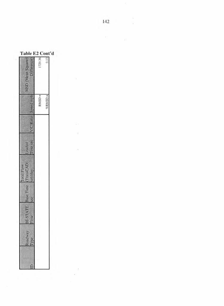
142
Table E2 Cont'd

143
APPENDIX F LINK COMPARISON TABLES
Table F1 Link ID 764 Comparisons
Run Number Link Length
{miles) Ruad~vay
Ciass Total Flotird
VMT Average
Speed mph. Average CCl
_gams Average
NOx gams Aver~icie HC
:grams
1 0.32 4 2,427 24 27,144 1,031 1,039 2 0.32 4 915 25 10,231 389 392 3 0.32 4 2,324 24 `26,000 987 995 4 0.32 4 917 25 10,257 390 393 5 0.32 4 2,255 24 25,224 958 966 6 0.32 4 1,043 24 11,664 443 446 7 0.32 4 2,188 24 24,474 929 937 8 0.32 4 2,188 24 24,474 929 937 9 0.32 4 2,507 22 28,048 1,065 1,074
10 0.32 4 1,520 24 16,999 646 651 11 0.32 4 2,409 19 28,161 1,081 1,129 12 0.32 4 1,792 20 20,948 804 840 13 0.32 4 2,031 20 23,738 9i 1 951 14 0.32 4 4,541 21 50,792 1,929 1,944 i 5 0.32 4 3,311 18 38,701 1,509 1,551 16 0.32 4 3,007 19 35,149 1,349 1,409 17 0.32 4 1,191 20 13,326 506 510 18 0.32 4 1,191 20 13,326 506 510 19 0.32 4 2,215 19 25,892 994 1,038 20 0.32 4 2, 541 24 29, 696 i ,140 1,190 21 0.32 4 1,971 24 22,051 837 844 22 0.32 4 2,360 25 26,400 1,003 1,011 23 0.32 4 2,460 24 27,518 1,045 i ,053 24 0.32 4 2,296 25 25,6$9 976 983 25 0.32 4 2,197 24 24,573 933 941 26 0.32 4 2,176 25 24,339 924 932 27 0.32 4 3,020 25 33,783 1,283 1,293 28 0.32 4 3,020 25 33,783 1,283 1,293 29 0.32 4 2,662 22 29,772 1,131 1,140
30 0.32 4 3,149 24 35,221 1,338 1,348

144
Table F2 Link ID 872 Comaarisons
fink Length (miles)
Roadway Class
Total Flow VMT
Average Speed m h
_~~ ~~__r~ ~ ~4verage NC)X grams
- - A~eragf~ HG=
rams =- F ~.
Run NumhGr Av -- ~__ _--
i 2.05 1 79,789 53 988,385 36,115 28,785
2 2.05 1 60,255 55 770,491 28,555 21,506
3 2.05 1 76;231 55 944,313. 34,544. 27,501
4 2.05 1 52,424 56 670,353 24,843 18,711
5 2.05 1 85,360 53 1,057,393 38,636 30,794
6 2.05 1 73,096 54 905,476 33,085 26,370
7 2.05 1 71,511 55 885,848 32,368 25,799
8 2.05 1 71,511 55 885,848 32,368 25,799 9 2.05 1 76,646 52 949,458 34,692 27,651
10 2.05 1 73,003 54 904,319 33,043 26,336
11 2.05 1 100,170 48 1,204,735 43,728 36,729
12 2.05 1 92,115 52 1,141,076 41,694 33,232
13 2.05 1 101,673 51 1,259,470 46,020 36,679
14 2.05 1 102,740 54 1,272,689 46,503 37,064
15 2.05 1 115,850 48 1,393,317 23,972 42,479 16 2.05 1 104,850 51 i ,298,825 47,458 37,826 17 2.05 1 92,972 54 1,151,695 42,082 33,541
18 2.05 1 92,972 54 1,151,695 42,082 33,541
19 2.05 1 103,803 48 1,248,430 45,314 38,062
20 2.05 1 104,569 52 1,295,344 47,331 37,724
21 2.05 1 70,847 53 877,616 32,067 25,559
22 2.05 1 82,107 55 7,049,918 38,910 29,305
23 2.05 1 90,513 54 1,121,235 40,969 32,654
24 2.05 1 69,018 56 882,544 32,707 24,633
25 2.05 1 79,446 54 984,132 35,959 28,661
26 2.05 1 71,163 55 909,975 33,724 25,399
27 2.05 1 68,058 56 870,280 32,253 24,291
28 2.05 1 68,058 56 870,280 32,253 24,291
29 2.05 i 83,773 54 1,037,738 37,918 30,222
30 2.05 1 73,379 55 938,313 34,774 26,190

145
Table F3 Link ID 1353 Comparisons
dirt , ~eng~h 'o~dway ~__,: Tout ov+f VMT
Average Average C~ T~~~ `
~_._ ',overage - Ox gams
Average- o - °F~u ~ 3-- = ~rniles) = lass ~,~ ~ °~ ~ ~rar
1
2
3
4
5
6
7
8
9
10
i 1
12
13
14
15 16
17
18
19
20
21
22
23
24
25
26
27
28
29
30
0.28
0.28
0.28
0.28
4
4
4
4
2,552 34 27,958 1,033 983
1,792
2,333
2,158
39
34
38
20,264
25,557
24,403
737
944
888
673
898
810
0.28 4 2,376 32 26,030 962 915
0.2$ 4 1,941 35 21,942 798 728
0.28 4 1,808 36 20,44 744 679
0.28 4 1,808 36 20,445 744 679
0.281 4 2,189 3 23,981 886 843
0.2 i ,792 35 20,263 737 673
0.28 4 2,307 32 25,278 934 889
0.28 4 2,403 34 26,322 972 925
0.28 4 2,249 33 24,635 910 866
0.28 4 2,884 36 32,604 1,186 1,082
0.28 2,501 31 27,396 6,608 963
0.28 4 2,55$ 33 28,022 1,035 9$5
0.2$ 4 3,069 36 34,698 1,262 1,152
0.28
0.28
0.28
4 3,06 • 36 34,698 1,262 1,152
4 _„_.2,322
2,16 •
_ z~~ _ 32
35
25,443
23, 704
_ „ yV_~_ 94
876
894
833
0.28 4 2,205 35 24,925 907 827
0.28 4 2,310 38 26,111 950 867
0.28 4 1,679 36 18,985 69i 630
0.28 4 2,511 37 28,385 1,033 942
0.28 4 2,240 35 25,329 921 841
0.28
0.28
4 2,265
2,410
38 25,607 932 850
39 27,245 991 904
0.28 4 2,410 39 27,245 991 904
0.28 4 2,009 35 22,714 826 754
0.28 4 2,518 37 28,468 i ,036 945

146
Table F4 Link ID 1711 Comaarisons
_ ? ~ ~ .~_.€ s ~
1 0.82 1 34,885 60 446,080 16,532 12,451
2 0.82 1 26,239 63 346,961 13,177 9,306 -: 3 0.82 1` 36,751 60 485,963 18,456 13,034
4 0.82 1 29,345 63 388,028 14,736 10,407
5 0.82 1 34,810 58 445,125 16,496 12,424
6 0.82 1 22,739 61 300,687 11,419 8,065
7 0.82 1 21,124 61 279,328 10,608 7,492
8 0.82 1 21,124 61 279,328 10,608 7,492
9 0.82 1 37,874 57 484,298 17,948 13,517
10 0.82 1 22,662 61 299,667 11,381 8,037
11 0.82 1 48,901 46 588,121 21,347 17,930
12 0.82 1 53,092 55 678,900 25,160 18,949
13 0.82 1 49,459 51 612,673 22,387 17,843 14 0.82 1 40,146 61 530,858 20,161 14,238
15 0.82 1 48,308 47 580,995 10,742 17,713 16 0.82 1 54,342 50 673,156 24,597 19,604
17 0.82 1 39,084 61 516,813 19,627 13,861 18 0.82 1 39,084 61 516,813 19,627 13,861
19 0.82 1 51,403 47 618,215 22,439 18,848
20 0.82 i 49,920 57 638,335 23,657 17,817
21 0.82 1 37,924 59 484,941 17,972 13,535 22 0.82 1 30,425 62 402,310 15,279 10,790 23 0.82 1 29,922 6 382,621 14,180 10,680 24 0.82 1 35,213 62 465,629 17,684 12,489
25 0.82 1 35,305 60 451,456 16,731 12,601
26 0.82 1, 33,202 62 439,036 16,674 11,775
27 0.82 1 23,867 63 315,597 11,986 8,465
28 0.82 1 23,867 63 315,597 11,986 8,465
29 0.82 1 34,187 59 437,152 16,201 12,202
30 0.82 1 34,461 62 455,686 17,306 12,222

Table FS Link ID 1851 Comparisons Linl<t~rtgth
~miies7
_ --Average
-~pead rr~#ah Averaged -per Average Averacl~; HC~
grams -_
_
Run (Number Roadwa~r
Class-:.
___ T~fa~Fiow
_ ~~viT =-=-~c i =gams
1 0.65 4 3,088 39 34,914 1,270
=
1,159 2 0.65 4 1,131 39 12,783 465 424
3 0.65 4 2,897 39 `32,748 1,19# 1,087 4 0.65 4 1,134 39 12,822 466 426
5 0.65 4 4,287 38 48,462 1,763 1,608 6 0.65 4 1,455 39 16,446 598 546
7 0.65 4 4,257 39 48,127 1,751 1,597 8 0.65 4 4,257 39 48,127 1,751 1,597
9 0.65 4 4,458 37 50,397 1,833 1,673 10 0.65 4 1,537 39 17,380 632 577 11 0.65 4 5,735 35 64,839 2,359 2,152 12 0.65 4 4,388 38 49,613 1,805 1,647 13 0.65 4 5,323 37 60,180 2,189 1,997 i 4 0.65 4 2,507 39 28,344 i ,031 941 15 0.65 4 6, i 91 34 67,828 1,788 2,384 16 0.65 4 6,222 37 70,340 2,559 2,335 17 0.65 4 6,707 39 75,831 2,759 2,517 18 0.65 4 6,707 39 75,831 2,759 2,517 19 0.65 4 5,733 35 64,810 2,358 2,151 20 0.65 4 4,603 38 52,041 1,893 1,727 21 0.65 4 2,$96 39 32,737 1,191 1,087 22 0.65 4 1,655 39 18,708 681 621 23 0.65 4 2,384 39 26,949 980 894 24 0.65 4 1,662 39 18,786 683 624 25 0.65 4 2,781 39 31,436 1,144 1,043 26 0.65 4 1,422 39 16,080 585 534 27 0.65 4 3,617 39 40,897 1,488 1,357 28 0.65 4 3,617 39 40,897 1,488 1,357 29 0.65 4 3,338 39 37,736 1,373 1,252
30 0.65 4 2,151 39 24,321 885 807

148
Table F6 Link ID 1911 Comparisons
dumber L"ink Length (miles
F~oadway Class V~T
Tatal Flow Average ~~e~l
Average CU grams . fly,
Average rams
Average H~; 9~~-~~ -.. T~.
1 0.76 5 2,331 32 25,532 943 897
2 0.76 5 1,952 32 ___ 21,382 _ _ 790 752 __ 3 0.76 5 2,3©0 32 ` 25,196 931 886
4 0.76 5 1,964 32 21,522 795 756
5 0.76 5 2,365 32 25,907 957 911
6 0.76 5 1,506 32 16,503 610 580
7 0.76 5 2,118 32 23,208 857 816
8 0.76 5 2,118 32 23,208 857 816
9 0.76 5 2,432 32 26,648 984 937
10 0.76 5 1,420 32 15,553 575 547
11 0.76 5 3,014 32 33,018 1,220 1,161
12 0.76 5 2,370 32 25,970 959 913
13 0.76 5 2,580 32 28,269 1,044 994
14 0.76 5 2,706 32 29,648 1,095 1,042
15 0.76 5 2,912 32 31,907 1,087 1,122
16 0.76 5 2,664 32 29,189 1,078 1,026 17 0.76 5 3,216 32 35,228 1,301 1,238
18 0.76 5 3,216 32 35,228 1,301 1,238
19 0.76 5 3,119 32 34,167 1,262 1,201
20 0.76 5 2,654 32 29,075 1,074 1,022
21 0.76 5 2,358 32 25,836 954 908 22 0.76 5 2,427 32 26,588 982 935
23 0.76 5 2,220 32 24,323 899 855 24 0.76 5 2,429 32 26,613 983 935
25 0.76 5 2,277 32 24,947 922 877
26 0.76 5 2,495 32 27,338 1,010 961
27 0.76 5 2,585 32 28,325 1,046 996
28 0.76 5 2,585 32 2$,325 1,046 996
29 0.76 5 2,268 32 24,852 918 874
30 0.76 5 2,463 32 26,985 997 949

149
Table F7 Link ID 1921- Comparisons
- - ~ Link
Le~~gth smiles)
o~ ~
Roadw a~~
~~lass s_
Toia6 Fio~AJ
<_ ~;YE!114T
Average Speed
_~~ph Average
CO grams..
AveragE~ NOx
grams _
Average HG
grams
perr,.entag e +,flange franc base ~ _.rase
z ~~ ~-.
~tn~i -~
1 1.77 4 8,021 42 93,615 3,386 2,946 1.53 2 1.77 4 4,310 42 50,300, 1,820 1,583 -45.45 3 1.77 4 7,900 42 92,202 3,335 2,901 fl4 1.77 4 4,272 42 49,852 1,803 1,569 -45.93 5 1.77 4 8,551 41 99;797 3,610 3,140 8.24
6 1.77 4 6,840 42 79,824 2,888 2,512 -13.42 7 1.77 4 5,478 42 63;928 2,313 2,012 -30.66 8 1.77 4 5,478 42 63,928 2,313 2,012 -30.66 9 1.77 4 9,899 41 115,527 4,179 3,635 25.3
10 1.77 4 6,894 42 80,460 2,911 2,532 -12.73 11 1.77 4 9,854 41 115,003 4,160 3,619 24.73 12 1.77 4 8,257 42 96,365 3,486 3,032 4.52 13 1.77 4 8,480 42 98.973 3,580 3,114 7.34 14 1.77 4 6,131 42 71,550 2,588 2,251 -22.4 15 1.77 4 9,634 41 112;439 2,468 3,538 21.95 16 1.77 4 9,090 42 106,090 3,838 3,338 15.06 17 1.77 4 6,351 42 74,124 2,681 2,332 -19.61 18 1.77 4 6,351 42 74,124 2,681 2,332 -19.61 19 1.77 4 9,889 41 115,409 4,175 3,631 25.17 20 1.77 4 8,091 42 94,429 3,416 2,971 2.42 21 1.77 4 6,849 42 79,931 2,891 2,515 -13.31 22 1.77 4 5,048 42 58,912 2,131 1,854 -36.11 23 1.77 4 7,029 42 82,030 2,967 2,581 -11.03 24 1.77 4 5,073 42 59,203 2,142 1,863 -35.79 25 1.77 4 6,913 42 80,685 2,919 2,539 -12.49 26 1.77 4 4,832 42 56,393 2,040 1,774 -38.84 27 1.77 4 4,934 42 57,578 2,083 1,812 -37.55 28 1.77 4 4,934 42 57,578 2,083 1,812 -37.55 29 1.77 4 7,336 42 85,618 3,097 2,694 -7.14
30 1.77 4 5,564 42 64;940 2,349 2,043 -29.57

150
Table F8 Link ID 2029 Comaarisons
Run Numbe
r
Link Length ~rr~il~
Roadwa Gass.-
~otaf F{ow VMT
Average - Speed
mph
Average Ct7
~r~s.:
Average Nix
grams~~
Average HC
~r~rr~_='
percent~~~ ; e chan~aE; -from ba~~e ''
case.;
1 0.88 4 6,826 39 77,172 2,807 2,561 0.48 2 0.88 4 5,249 41 61,262 2,216 1,928 -20.24 3 0.88 4 6,794 39 76;807 2;794 2,549 0 4 0.88 4 5,253 41 61,309 2,218 1,929 -20.18 5 0.88 4 6,793 37 76,802 2,794 2,549 -0.01 6 0.88 4 5,657 40 63,961 2,327 2,123 -16.72 7 0.88 4 5,592 40 65,268 2,361 2,054 -i 5.02 8 0.88 4 5,592 40 65,268 2,361 2,054 -15.02 9 0.88 4 6,572 37 74,302 2,703 2,466 -3.26
10 0.88 4 5,420 40 61,276 2,229 2,034 -20.22 11 0.$8 4 7,087 36 80,124 2,915 2,659 4.32 12 0.88 4 7,182 39 81,194 2,954 2,695 5.71 13 0.88 4 7,180 37 81,172 2,953 2,694 5.68 14 0.88 4 6,991 40 81,591 2,951 2,567 6.23 15 0.88 4 7,123 36 80,528 1,468 2,673 4.84 16 0.88 4 7,152 37 80,857 2,941 2,684 5.27 17 0.88 4 6,933 40 80,916 2,927 2,546 5.35 i8 0.88 4 6,933 40 80,916 2,927 2,546 5.35 i9 0.$8 4 7,089 36 80,147 2,916 2,660 4.35 20 0.88 ~ 4 7,137 39 80,685 2,935 2,678 5.05 21 0.88 4 6,841 38 77,342 2,814 2,567 0.7 22 0.88 4 6,334 41 73,920 2,674 2,326 -3.76 23 0.88 4 6,849 38 77,431 2,817 2,570 0.81 24 0.88 4 6,337 41 73,956 2,675 2,327 -3.71 25 0.88 4 6,855 38 77,495 2,819 2,572 0.9 26 0.88 4 6,214 41 72,519 2,623 2,282 -5.58 27 0.88 4 6,344 42 74,042 2,678 2,330 -3.6 28 0.88 4 6,344 42 74,042 2,678 2,330 -3.6 29 0.88 4 6,570 39 74,281 2,702 2,465 -3.29
30 0.88 4 6,357 41 74,193 2,684 2,335 -3.4

151
Table F9 Link ID 2040 Comparisons
Run Num
Link Length; .
, ~~ Raadtiva =Mass ::.
Total Flow
~;1/MT
Average Speed mph~~r~r~s
Average CO
Average NOx
gams_
~. =~ ~ percentag
e change from base tease ~ ~,,;-
_~ ; Average
HC z~ram~ ~
1 2.04 1 34,640 63 458,045 17,396 12,285 0
2 2.04 1 33,870 63 447,869 i 7,009 i 2,012 -2.22
3 2:04 -i 34,640 63 . 458,045 17,396 12,285. 0 4 2.04 1 33,870 63 447,869 17,009 12,012 -2.22
5 2.04 1 34,640 63 458,045 17,396 12,285 0
6 2.04 1 33,870 63 447,869 17,009 i 2,012 -2.22
7 2.04 1 33,870 63 447,869 17,009 i 2,012 -2.22
8 2.04 i 33,870 63 447,869 17,009 12,012 -2.22
9 2.04 1 34,640 63 458,045 17,396 12,285 0
10 2.04 1 33,870 63 447,869 17,009 12,012 -2.22
11 2.04 1 34,640 63 458,045 17,396 12,285 0
12 2.04 1 34,640 63 458,045 17,396 12,285 0
13 2.04 1 34,640 63 458,045 17,396 12,285 0 14 2.04 1 34,640 63 458,045 17,396 12,2$5 0 15 2.04 1 34,640 63 458,045 9,414 12,285 -2.3 16 2.04 1 34,640 63 458,045 17,396 12,285 0 17 2.04 1 34,640 63 458,045 17,396 12,285 0
18 2.04 1 34,640 63 458,045 17,396 12,285 0 19 2.04 1 34,640 63 458,045 17,396 12,285 0 20 2.04 1 34,640 63 458,045 17,396 12,285 0 21 2.04 1 34,640 63 458,045 17,396 12,285 0 22 2.04 1 34,640 63 458,045 17,396 12,285 0 23 2.04 1 34,640 63 458,045 17,396 12,285 0 24 2.04 1 34,640 63 458,045 17,396 12,285 0 25 2.04 1 34,640 63 458,045 17,396 12,285 0
26 2.04 1 34,640 63 458,045 17,396 12,285 0 27 2:04 1 34,640 63 458,045 17,396 12,285 0 28 2.04 1 34,640 63 458,045 17,396 12,285 0 29 2.04 1 34,640 63 458,045 17,396 12,285 0
30 2.04 1 34,640 63 458,045 17,396 12,285 0

152
Table F10 Link ID 2053 Comparisons _~.~
~y,Run glum r ~= ber
Roadvva y Class
0
Tata! Flow VMT
Average fVOx
-=9 rams ._
Average H~C urns
percentag e change frat~~ base
case
Link Length {miles)
Averages ~verage Speec(~- ~© 3`
-_ . ~nph. -~- rams ~
1 0.92 4 3,576
_
42 41,731 1,510 1,313 0
2 0.92 4 3,268 42 38,138 1,380 1,200 -8.61
3 0.92 4 3,576 42 41,731 1,510 1,313 0
4 0.92 4 3,268 42 38,138 1,380 1,200 -8.61
5 0.92 4 3,576 42 41,731 1,510 1,313 0
6 0.92 4 3,268 42 38,138 1,380 1,200 -8.61
7 0.92 4 3,268 42 38,138 1,380 1,200 -8.61
8 0.92 4 3,268 42 38,138 1,380 1,200 -8.61
9 0.92 4 3,576 42 41,731 1,510 1,313 0
10 0.92 4 3,268 42 38,138 1,380 1,200 -8.61
11 0.92 4 3,576 42 41,731 1,510 1,313 0
12 0.92 4 3,576 42 41,731 1,510 1,313 0
13 0.92 4 3,576 42 41,731 1,510 1,313 0
14 0.92 4 3,576 42 41,731 1,510 1,313 0
15 0.92 4 3,576 42 41,731 1,510 1,313 0
16 0.92 4 3,576 42 41,731 1,510 1,313 0
17 0.92 4 3,576 42 41,731 1,510 1,313 0
18 0.92 4 3,576 42 41.731 1,510 1,3i 3 0
19 0.92 4 3,576 42 41,731 1,510 1,313 0
20 0.92 4 3,576 42 41,731 1,510 1,313 0
21 0.92 4 3,576 42 41,731 1,510 1,313 0
22 0.92 4 3,576 42 41,731 1,510 1,313 0
23 0.92 4 3,576 42 41,731 1,510 1,313 0
24 0.92 4 3,576 42 41,731 1,510 1,313 0
25 0.92 4 3,576 42 41,731 1,510 1,313 0
26 0.92 4 3,576 42 41,731 1,510 1,313 0 27 0.92 4 3,576 42 41.731 1,510 1,313 0
28 0.92 4 3,576 42 41,731 1,510 1,313 0
29 0.92 4 3,576 42 41.731 1,510 1,313 0
30 0.92 4 3,576 42 41,731 1,510 1,313 0
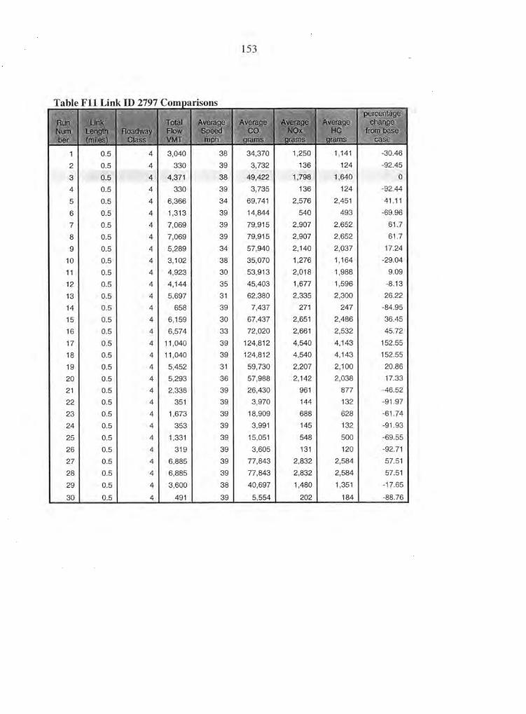
Table F11 Link ID 2797 Comparisons
Run Num ~e~~„ ales)
Link ~ Lengih Roadway
Class
"fatal Flovu
~~T
Average Speed
r+~~.:.:,~
- - ~- ~~verage
HG - ~r.~r~s~ -
percentage charge
from base Cass
Average CQ
_ ~
= _ ge -iVOx
==,~ramS
1 0.5 4 3,040 38 34,370 1,250 i ,141 -30.46
2 0.5 4 330 39 3,732 136 124 -92.45
3 0.5 4 4,371 38 49,422 1..,798 1,640: . . - 0
4 0.5 4 330 39 3,735 i 36 124 -92.44
5 0.5 4 6,366 34 69,741 2,576 2,451 41.11
6 0.5 4 1,313 39 14,844 540 493 -69.96
7 0.5 4 7,069 39 79,915 2,907 2,652 61.7
8 0.5 4 7,069 39 79,915 2,907 2,652 61.7
9 0.5 4 5,289 34 57,940 2,140 2,037 17.24
10 0.5 4 3,102 38 35,070 1,276 1,164 -29.04
11 0.5 4 4,923 30 53,913 2,018 1,988 9.09
12 0.5 4 4,144 35 45,403 1,677 1,596 -8.13
13 0.5 4 5,697 31 62,380 2,335 2,300 26.22
14 0.5 4 658 39 7,437 271 247 -84.95
15 0.5 4 6,159 30 67,437 2,651 2,486 36.45 16 0.5 4 6,574 33 72,020 2,661 2,532 45.72
17 0.5 4 11, 040 39 124, 812 4, 540 4,143 152.55
18 0.5 4 11,040 39 124,812 4,540 4,143 152.55
19 0.5 4 5,452 31 59,730 2,207 2,100 20.86 20 0.5 4 5,293 36 57,988 2,142 2,038 17.33 21 0.5 4 2,338 39 26,430 961 877 -46.52
22 4.5 4 351 39 3,970 144 132 -91.97
23 0.5 4 1,673 39 18,909 688 628 -61.74 24 0.5 4 353 39 3,991 145 132 -91.93
25 0.5 4 1,331 39 15,051 548 500 -69.55
26 0.5 4 319 39 3,605 131 120 -92.71 27 0.5 4 6,885 39 77,843 2,832 2,584 57.51
28 0.5 4 6,885 39 77,843 2,832 2,584 57.51
29 0.5 4 3,600 38 40,697 1,480 1,351 -17.65
30 0.5 4 491 39 5,554 202 184 -88.76

I~~
Table F12 Link ID 2936 Comparisons -- =
Road~v~ay Cta~~~
Total F(ow
Average Speed
~~'•~
~-
Average CO ~rr~s
Average NOx
grat~s ~
- Aveta~e
HC grams
percentage ' change
from base case..
=. -
Run Nur~ ~niles',~
L(nK Lengtt►
1 0.52 4 6921 40 80776 2922 2542 -3.05
2 0.52 4 5270 41 61506 2225 1935 -26.18
3 0.52 4 7139 40 ' 83317 3014 2622. 0
4 0.52 4 5140 41 59992 2170 1888 -28
5 0.52 4 6789 40 76759 2792 2548 -6.02
6 0.52 4 5010 41 58465 2115 1840 -29.83
7 0.52 4 3766 41 43952 1590 1383 -47.25
8 0.52 4 3766 41 43952 1590 1383 -47.25
9 0.52 4 6019 40 70244 2541 2210 -15.69
10 0.52 4 2355 . 41 27486 994 865 -67.01
11 0.52 4 6891 39 77907 2834 2586 -4.61
12 0.52 4 7954 40 89925 3271 2985 10.11
13 0.52 4 6620 40 74839 2723 2484 -8.37
14 0.52 4 8271 41 96525 3492 3037 15.85
15 0.52 4 6671 39 75418 6802 2503 37.23
16 0.52 4 5602 40 63339 2304 2102 -22.45
17 0.52 4 5343 41 62352 2255 1962 -25.16
18 0.52 4 5343 41 62352 2255 1962 -25.16
19 0.52 4 5860 40 66246 2410 2199 -18.89 20 0.52 4 7187 40 83872 3034 2639 0.67
21 0.52 4 6400 41 74696 2702 2350 -10.35
22 0.52 4 6313 41 73672 2665 2318 -11.58 23 0.52 4 6408 41 74791 2705 2353 -10.23 24 0.52 4 6512 41 76001 2749 2391 -8.78
25 0.52 4 6274 41 73223 2649 2304 -12.12
26 0.52 4 6762 41 78915 2855 2483 -5.28 27 0.52 4 4808 42 56114 2030 1766 -32.65
28 0.52 4 4808 42 56114 2030 1766 -32.65 29 0.52 4 5528 41 64515 2334 2030 -22.57
30 0.52 4 5479 41 63940 2313 2012 -23.26

155
APPEN~TI~-G BI-STATE MODEL FIL-ES
The following files are included in the accompanying CD. They were obtained from the Bi-
State Commission during the initial phases of the research undertaken.
• 1998attr.f98 • 1998prod.f98 • Eetab.98 • Ffr2.dat • Hnet l .f98 • Hrldxyi3.f98 • Run98f. in • Ttprep . tem • Turn. txt • Ttprep. tem • 2025attr.f25 • 2025prod.f25 • Eetab.25 • Ffr2. dat • Hnet l .f25
• Hrldxyi3.f25 • Run25f.in • Turn.txt • Netcard.exe
Year 1998 Attraction file in Tranplan format; Year 1998 Production file in Tranplan format; Year 1998 Ext — Ext trip table; Friction factor file; Year 199$ Base Network; Year 1998 initial network. This network is used to skim paths; Year 1998 Tranplan control file; Terminal time for all Traffic Analysis Zones; Year 1998 Turn penalty file. Terminal time for all Traffic Analysis Zones; Year 2025 Attraction file in Tranplan format; Year 2025 Production file in Tranplan format; Year 2025 Ext — Ext trip table; Friction factor file; Year 2025 Base Network. This includes year 2025 Transportation Projects; Year 2025 initial network. This network is used to skim paths; Year 2025 Tranplan control file; Year 2025 Turn penalty file;
The non..f98 and .f25 files can be accessed by use of standard text editors available in the
Microsoft Windows personal computer environment. The Netcard.exe is run in a command
line (DOS) mode and returns a flat text file able to be viewed in standard text editors.

156
REFERENCES
1, Environmental 1-Iealth Center. Air Pollution Fact Sheet (for Ne~v Drivers) April 7, 2003. http:/~www.nsc.orglehc/mobile/airpollu.htm Accessed May 5, 2003
2. Natural Resources Defense Council. Clean Air and Energy: Particulate Pollution. May ~, 1996. http:I/www.nrdc.or~/air/pollutionlgbreath.asp Accessed May 6, 2003
3. Union of Concerned Scientists Clean Vehicle website. March 26, 2003, http:Ilwvvw.ucsusa.orglclean_vehicles/index.cfm. Accessed March 31, 2003,
4. U. S Environmental Protection Agency website. www. epa. gov Accessed May 9, 2003
5. Stacy C. Davis and Susan W. Diegel, U.S Department of Energy Transportation Energy Data Book: Edition 22 Chapter 2. September, 2002.
6. Lydia M. Wiegman. Status of B-IIour Ozone and PM2.S Standards. STAPPA I ALAPCO Meeting. Stowe, Vermont, September 30,2002
7. Simon Washington and Randall Guensler. Modeling Air Quality for Conformity, Current Deficiencies, and New Directions. UCTC No. 98. University of California Transportation Center. UC Berkeley.
8. Matthew Barth and Carrie Malcolm, George Scora. Integrating a Comprehensive Modal Emissions Model into ATMIS Transportation Modeling Frameworks. California Path Program, Institute of Transportation Studies, University of California Berkeley. August 2001.
9. Edward A. Beimborn. A Transportation Modeling Primer. Center for Urban Transportation Studies University of Wisconsin-Milwaukee 1995.
10. Martin, W.A. and N.A. McGuckin. NCHRP Report 365: Travel Estimation Techniques for Urban Planning. Transportation Research Board, National Academy Press, Washington D.C. 1998.
11. TransCAD TDM (Travel Demand Modeling with TransCAD 4.0). Caliper Corporation Copyright 2000
12. Deakin, Harvey and Skabardonis, Berkeley, CA. Manual of Regional Transportation Modeling Practice for Air Quality Analysis. TMiP 1993.
13. John Bowman, Thomas Rossi, Earl Ruiter, Kevin Tierney, David Kurth, and William Martin. Short-Term Travel Model Improvements. Chapter 1 Final Report October 1994. USDOT.

157
14. Harvey J. Miller. Towards Consistent Travel Demand Estimation in Transportation Planning: A Guide to the Theory and Practice of Equilibrium Travel Demand Modeling. Department of Geography, University of Utah, November 1997.
15. Calibrating and Adjustment of System Planning Models -December 1990. Bureau of Transportation Statistics, National Transportation Library.
16. Model Validation and Peasonableness Checking Manual. Prepared by Barton-Aschman Associates, Inc. Cambridge Systematics, inc. for Travel Model Improvement Program Federal ~-Iighway Administration. February 1997.
17. TRANSI~vIS web page. http://transims.tsasa.lanl.govl Last accessed May 11, 2003.
18. Los Alamos National Laboratory. TRANS IMS 3.0 Documentation. March 2, 2002.
19. Bi-State Regional Commission website. www.bistateonline.org Accessed March 23, 2003 .
20. Citilabs website, Tranplan section. http://www.citilabs.com/tranplanl Accessed April 8, 2003.
21. Caliper Corporation's TransCAD website http://www.caliper,com/tcovu.htm Accessed Aprii 492003.
22. Barry T. Meyer. Sensitivity Vesting and Analysis. EG&G Mound Applied Technologies. June 1991
23. Kenneth Warp, Cecil F. Warner, and Wayne T. Davis. Air Pollution, Its Origin and Control 3~d Edition. Addison Wesley Longman, Inc.
24. U.S. Environmental Protection Agency EPA user's Guide to MOBILE b.0 Mobile source Emission Factor Model. January 2002.\
25. Iowa Department of Natural Resources web site. Energy Section. http://www.state.ia.us/dnr/energy/index.htm Last accessed. Last accessed May 13, 2003 .
26. Renewable Fuels Association. Fuel Ethanol. Industry Guidelines, S~eci~ fications and Procedures. Page 4 RFA Publication #960501, 1VIay 2002.
27. Alan Agresti and Barbara Finlay. ►Statistical Methods for the Social Sciences ~r~
Edition. Prentice Hall, Upper Saddle River, New Jersey, 1997.

158
28. James Hampton. Lectures on Statistics (Analysis of Variance) October 22, 2002. http:llwww.staff.city.ac.u~/hampton~stats_lectures.htm. Accessed April 29, 2003.
29. Mark Torrance. Introduction to Analysis of Variance. Assumptions for ANOVA and what to do if they are violated. September 26, 2002. http:llwww.staffs.ac.uk/personal/sciences/smt15/mt15/rm3/index.html Accessed May 2, 2003
30. Modeling 1Vlobile Source Emissions. Wage ~ 7. Natural Academies Press. Copyright 2000.
31. TransCAD user's Guide. Caliper Corporation Copyright 2000
32. Improving Transportation Data for Mobile Source Emission Estimates. deport 394. National Academy Press . 1997 .
3 3 . Rodier, CJ, Johnston, RA. ~Incertain ►Socioeconomic ~'rojections used in Travel Demand and emissions Models: could plausible errors result in Air Quality ~VonConformity? Journal Title: Transportation Research. Part A: Policy and Practice volume 36 Issue 7, Elsevier Science, Limited 2002.
34. Reginald D. Dolledge and Tommy Darling. Spatial Behavior in Transportation Modeling and Planning and Modeling. Department of Geography and Research Unit on Spatial Cognition and Choice. UCSB (University of California Santa Barbara. Department of Psychology, Goteborg University, Goteborg, Sweden. June 4, 2001.
3 5. U. S . Department of Transportation. Transportation Model Improvement Program. http://tmip.fhwa.dot.gov/ Accessed March 29, 2003.
36. Broadway Historic District website. http:Ilwww.broadwaydistrict.org/maps,htmAccessed May 28, 2003.