Sensitivity Analysis - Aerospace Design Laboratoryadl.stanford.edu/.../chapter4_sensitivity.pdf · 2012-04-16 · AA222: MDO 77 Friday 6th April, 2012 at 12:06 Chapter 4 Sensitivity

AA222: MDO 77 Friday 6th April, 2012 at 12:06

Chapter 4

Sensitivity Analysis

4.1 Introduction

Sensitivity analysis consists in computing derivatives of one or more quantities (outputs) with re-spect to one or several independent variables (inputs). Although there are various uses for sensitiv-ity information, our main motivation is the use of this information in gradient-based optimization.Since the calculation of gradients is often the most costly step in the optimization cycle, usingefficient methods that accurately calculate sensitivities is extremely important.

Consider a general constrained optimization problem of the form:

minimize f(xi)

w.r.t xi i = 1, 2, . . . , n

subject to cj(xi) ≥ 0, j = 1, 2, . . . ,m

(4.1)

In order to solve this problem using a gradient-based optimization algorithm we usually require:

• The sensitivities of the objective function, ∇f(x) = ∂f/∂xi (n× 1).

• The sensitivities of all the active constraints at the current design point ∂cj/∂xi (m× n).

4.2 Motivation

By default, most gradient-based optimizers use finite-differences for sensitivity analysis. This isboth costly and subject to inaccuracies.

When the cost of calculating the sensitivities is proportional to the number of design variables,and this number is large, sensitivity analysis is the bottleneck in the optimization cycle.

Accurate sensitivities are required for convergence.

4.2.1 Methods for Sensitivity Analysis

Finite Differences: very popular; easy, but lacks robustness and accuracy; run solver n times.

Complex-Step Method: relatively new; accurate and robust; easy to implement and maintain;run solver n times.

Symbolic Differentiation: accurate; restricted to explicit functions of low dimensionality.


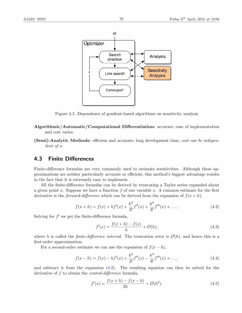
Figure 4.1: Dependence of gradient-based algorithms on sensitivity analysis

Algorithmic/Automatic/Computational Differentiation: accurate; ease of implementationand cost varies.

(Semi)-Analytic Methods: efficient and accurate; long development time; cost can be indepen-dent of n.

4.3 Finite Differences

Finite-difference formulae are very commonly used to estimate sensitivities. Although these ap-proximations are neither particularly accurate or efficient, this method’s biggest advantage residesin the fact that it is extremely easy to implement.

All the finite-difference formulae can be derived by truncating a Taylor series expanded abouta given point x. Suppose we have a function f of one variable x. A common estimate for the firstderivative is the forward-difference which can be derived from the expansion of f(x+ h),

f(x+ h) = f(x) + hf ′(x) +h2

2!f ′′(x) +

h3

3!f ′′′(x) + . . . , (4.2)

Solving for f ′ we get the finite-difference formula,

f ′(x) =f(x+ h)− f(x)

h+O(h), (4.3)

where h is called the finite-difference interval. The truncation error is O(h), and hence this is afirst-order approximation.

For a second-order estimate we can use the expansion of f(x− h),

f(x− h) = f(x)− hf ′(x) +h2

2!f ′′(x)− h3

3!f ′′′(x) + . . . , (4.4)

and subtract it from the expansion (4.2). The resulting equation can then be solved for thederivative of f to obtain the central-difference formula,

f ′(x) =f(x+ h)− f(x− h)

2h+O(h2). (4.5)


x x+h

f(x)

f(x+h)

Figure 4.2: Graphical representation of the finite difference approximation

More accurate estimates can also be derived by combining different Taylor series expansions.

Formulas for estimating higher-order derivatives can be obtained by nesting finite-differenceformulas. We can use, for example the central difference (4.5) to estimate the second derivativeinstead of the first,

f ′′(x) =f ′(x+ h)− f ′(x− h)

2h+O(h2). (4.6)

and use central difference again to estimate both f ′(x+ h) and f ′(x− h) in the above equation toobtain,

f ′′(x) =f(x+ 2h)− 2f(x) + f(x− 2h)

4h2+O(h). (4.7)

When estimating sensitivities using finite-difference formulae we are faced with the step-sizedilemma, that is the desire to choose a small step size to minimize truncation error while avoidingthe use of a step so small that errors due to subtractive cancellation become dominant.

Forward-difference approximation:

df(x)

dx=f(x+ h)− f(x)

h+O(h). (4.8)

With 16-digit arithmetic,

f(x+ h) +1.234567890123431f(x) +1.234567890123456∆ f −0.000000000000025

For functions of several variables, that is when x is a vector, then we have to calculate eachcomponent of the gradient ∇f(x) by perturbing the corresponding variable xi.

The cost of calculating sensitivities with finite-differences is therefore proportional to the numberof design variables and f must be calculated for each perturbation of xi. This means that if we useforward differences, for example, the cost would be n+ 1 times the cost of calculating f .


4.4 The Complex-Step Derivative Approximation

4.4.1 Background

The use of complex variables to develop estimates of derivatives originated with the work of Lynessand Moler [12] and Lyness [13]. Their work produced several methods that made use of complexvariables, including a reliable method for calculating the nth derivative of an analytic function.However, only recently has some of this theory been rediscovered by Squire and Trapp [22] andused to obtain a very simple expression for estimating the first derivative. This estimate is suitablefor use in modern numerical computing and has shown to be very accurate, extremely robust andsurprisingly easy to implement, while retaining a reasonable computational cost [14, 15].

4.4.2 Basic Theory

We will now see that a very simple formula for the first derivative of real functions can be obtainedusing complex calculus. The complex-step derivative approximation can also be derived using aTaylor series expansion. Rather than using a real step h, we now use a pure imaginary step, ih.If f is a real function in real variables and it is also analytic, we can expand it in a Taylor seriesabout a real point x as follows,

f(x+ ih) = f(x) + ihf ′(x)− h2 f′′(x)

2!− ih3 f

′′′(x)

3!+ . . . (4.9)

Taking the imaginary parts of both sides of (4.9) and dividing the equation by h yields

f ′(x) =Im [f(x+ ih)]

h+ h2 f

′′′(x)

3!+ . . . (4.10)

Hence the approximations is a O(h2) estimate of the derivative of f .An alternative way of deriving and understanding the complex step is to consider a function,

f = u + iv, of the complex variable, z = x + iy. If f is analytic the Cauchy–Riemann equationsapply, i.e.,

∂u

∂x=∂v

∂y(4.11)

∂u

∂y= −∂v

∂x. (4.12)

These equations establish the exact relationship between the real and imaginary parts of the func-tion. We can use the definition of a derivative in the right hand side of the first Cauchy–Riemannequation (4.11) to obtain,

∂u

∂x= lim

h→0

v(x+ i(y + h))− v(x+ iy)

h. (4.13)

where h is a small real number. Since the functions that we are interested in are real functions of areal variable, we restrict ourselves to the real axis, in which case y = 0, u(x) = f(x) and v(x) = 0.Equation (4.13) can then be re-written as,

∂f

∂x= lim

h→0

Im [f (x+ ih)]

h. (4.14)

For a small discrete h, this can be approximated by,

∂f

∂x≈ Im [f (x+ ih)]

h. (4.15)


We will call this the complex-step derivative approximation. This estimate is not subject to sub-tractive cancellation error, since it does not involve a difference operation. This constitutes atremendous advantage over the finite-difference approaches expressed in (4.3, 4.5).

Example 4.10. The Complex-Step Method Applied to a Simple FunctionTo show the how the complex-step method works, consider the following analytic function:

f(x) =ex√

sin3 x+ cos3 x(4.16)

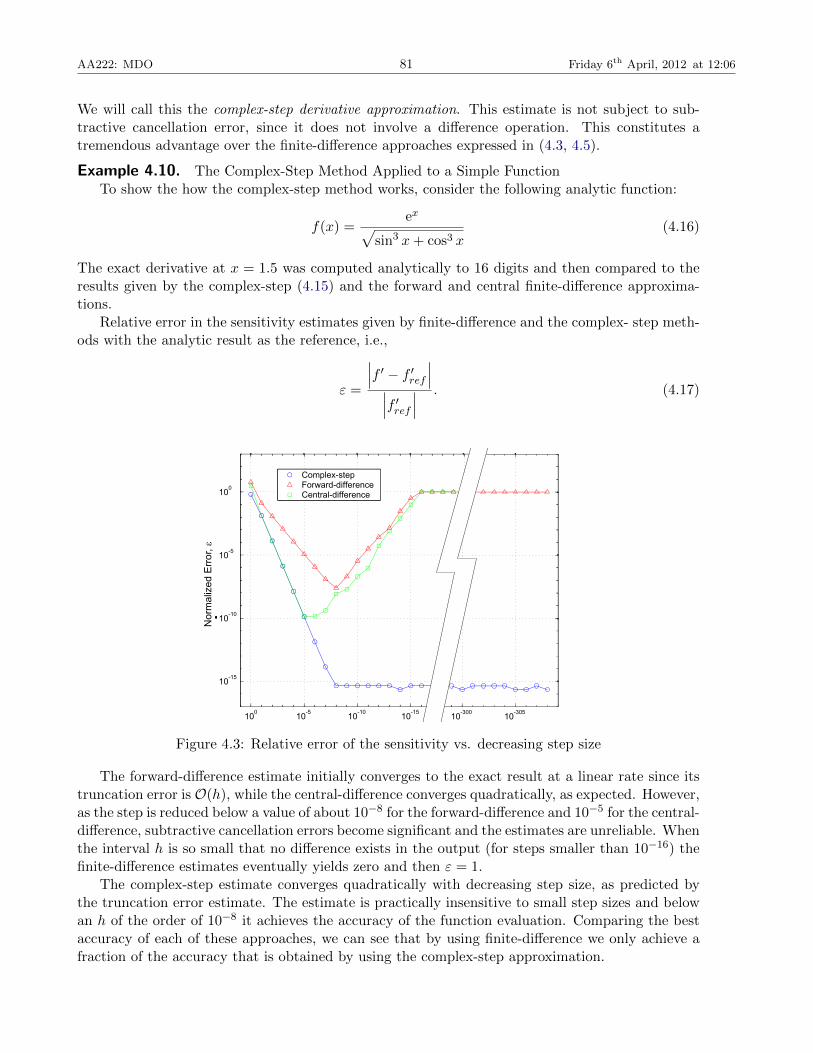
The exact derivative at x = 1.5 was computed analytically to 16 digits and then compared to theresults given by the complex-step (4.15) and the forward and central finite-difference approxima-tions.

Relative error in the sensitivity estimates given by finite-difference and the complex- step meth-ods with the analytic result as the reference, i.e.,

ε =

∣∣∣f ′ − f ′ref ∣∣∣∣∣∣f ′ref ∣∣∣ . (4.17)

Step Size, h

No

rma

lize

d E

rro

r,e

Figure 4.3: Relative error of the sensitivity vs. decreasing step size

The forward-difference estimate initially converges to the exact result at a linear rate since itstruncation error is O(h), while the central-difference converges quadratically, as expected. However,as the step is reduced below a value of about 10−8 for the forward-difference and 10−5 for the central-difference, subtractive cancellation errors become significant and the estimates are unreliable. Whenthe interval h is so small that no difference exists in the output (for steps smaller than 10−16) thefinite-difference estimates eventually yields zero and then ε = 1.

The complex-step estimate converges quadratically with decreasing step size, as predicted bythe truncation error estimate. The estimate is practically insensitive to small step sizes and belowan h of the order of 10−8 it achieves the accuracy of the function evaluation. Comparing the bestaccuracy of each of these approaches, we can see that by using finite-difference we only achieve afraction of the accuracy that is obtained by using the complex-step approximation.


The complex-step size can be made extremely small. However, there is a lower limit on thestep size when using finite precision arithmetic. The range of real numbers that can be handled innumerical computing is dependent on the particular compiler that is used. In this case, the smallestnon-zero number that can be represented is 10−308. If a number falls below this value, underflowoccurs and the number drops to zero. Note that the estimate is still accurate down to a step of theorder of 10−307. Below this, underflow occurs and the estimate results in NaN.

Comparing the accuracy of complex and real computations, there is an increased error in basicarithmetic operations when using complex numbers, more specifically when dividing and multiply-ing.

4.4.3 New Functions and Operators

To what extent can the complex-step method be used in an arbitrary algorithm? To answer thisquestion, we have to look at each operator and function in the algorithm.

• Relational operators

– Used with if statements to direct the execution thread.

– Complex algorithm must follow same thread.

– Therefore, compare only the real parts.

– Also, max, min, etc.

• Arithmetic functions and operators:

– Most of these have a mathematical standard definition that is analytic.

– Some of them are implemented in Fortran.

– Exception: abs

∂u

∂x=∂v

∂y=

{−1 ⇐ x < 0

+1 ⇐ x > 0(4.18)

abs(x+ iy) =

{−x− iy ⇐ x < 0

+x+ iy ⇐ x ≥ 0. (4.19)

4.4.4 Can the Complex-Step Method be Improved?

Improvements necessary because,

arcsin(z) = −i log[iz +

√1− z2

], (4.20)

may yield a zero derivative. . .How? If z = x+ ih, where x = O(1) and h = O(10−20) then in the addition,

iz + z = (x− h) + i (x+ h) (4.21)

h vanishes when using finite precision arithmetic.Would like to keep the real and imaginary parts separate.The complex definition of sine also problematic,

sin(z) =eiz − e−iz

2i. (4.22)


The complex trigonometric relation yields a better alternative,

sin(x+ ih) = sin(x) cosh(h) + i cos(x) sinh(h). (4.23)

Note that linearizing this equation (that is for small h) this simplifies to,

sin(x+ ih) ≈ sin(x) + ih cos(x). (4.24)

From the standard complex definition,

arcsin(z) = −i log[iz +

√1− z2

]. (4.25)

Need real and imaginary parts to be calculated separately.Linearizing in h about h = 0,

arcsin(x+ ih) ≡ arcsin(x) + ih√

1− x2. (4.26)

4.4.5 Implementation Procedure

• Cookbook procedure for any programming language:

– Substitute all real type variable declarations with complex declarations.

– Define all functions and operators that are not defined for complex arguments.

– A complex-step can then be added to the desired variable and the derivative can beestimated by f ′ ≈ Im[f(x+ ih)]/h.

• Fortran 77: write new subroutines, substitute some of the intrinsic function calls by thesubroutine names, e.g. abs by c abs. But. . . need to know variable types in original code.

• Fortran 90: can overload intrinsic functions and operators, including comparison operators.Compiler knows variable types and chooses correct version of the function or operator.

• C/C++: also uses function and operator overloading.

4.4.6 Fortran Implementation

• complexify.f90: a module that defines additional functions and operators for complex ar-guments.

• Complexify.py: Python script that makes necessary changes to source code, e.g., type dec-larations.

• Features:

– Script is versatile:

∗ Compatible with many more platforms and compilers.

∗ Supports MPI based parallel implementations.

∗ Resolves some of the input and output issues.

– Some of the function definitions were improved: tangent, inverse and hyperbolic trigono-metric functions.


Figure 4.4: Aerostructural solution for the supersonic business jet

4.4.7 C/C++ Implementations

• complexify.h: defines additional functions and operators for the complex-step method.

• derivify.h: simple automatic differentiation. Defines a new type which contains the valueand its derivative.

Templates, a C++ feature, can be used to create program source code that is independent ofvariable type declarations.

• Compared run time with real-valued code:

– Complexified version: ≈ ×3

– Algorithmic differentiation version: ≈ ×2

Example 4.11. 3D Aero-Structural Design Optimization Framework [16]

• Aerodynamics: SYN107-MB, a parallel, multiblock Navier–Stokes flow solver.

• Structures: detailed finite element model with plates and trusses.

• Coupling: high-fidelity, consistent and conservative.

• Geometry: centralized database for exchanges (jig shape, pressure distributions, displace-ments.)

• Coupled-adjoint sensitivity analysis

Example 4.12. Supersonic Viscous/Inviscid Solver [23]Framework for preliminary design of natural laminar flow supersonic aircraft

• Transition prediction


100 200 300 400 500 600 700 80010

−8

10−6

10−4

10−2

100

Iterations

Ref

eren

ce E

rror

, ε

CD

∂ C

D / ∂ b

1

Figure 4.5: Convergence of CD and ∂CD/∂b1

10−15

10−10

10−5

10−6

10−5

10−4

10−3

10−2

10−1

100

Rel

ativ

e E

rror

, ε

Step Size, h

Complex−Step Finite−difference

Figure 4.6: Sensitivity estimate vs. step size. Note that the finite-difference results are practicallyuseless.


2 4 6 8 10 12 14 16 18

−0.05

0

0.05

0.1

0.15

∂ C

D /

∂ b i

Shape variable, i

Complex−Step, h = 1×10−20 Finite−Difference, h = 1×10−2

Figure 4.7: Sensitivity of CD to shape functions. The finite-different results were obtained aftermuch effort to choose the best step.

• Viscous and inviscid drag

• Design optimization

– Wing planform and airfoil design

– Wing-Body intersection design

• Python wrapper defines geometry

• CH GRID automatic grid generator

– Wing only or wing-body

– Complexified with our script

• CFL3D calculates Euler solution


Figure 4.8: CFD grid

– Version 6 includes complex-step

– New improvements incorporated

• C++ post-processor for the. . .

• Quasi-3D boundary-layer solver

– Laminar and turbulent

– Transition prediction

– C++ automatic differentiation

• Python wrapper collects data and computes structural constraints

4.5 Automatic Differentiation

Automatic differentiation (AD) — also known as computational differentiation or algorithmic dif-ferentiation — is a well known method based on the systematic application of the differentiationchain rule to computer programs. Although this approach is as accurate as an analytic method, itis potentially much easier to implement since this can be done automatically.

4.5.1 How it Works

The method is based on the application of the chain rule of differentiation to each operation in theprogram flow. The derivatives given by the chain rule can be propagated forward (forward mode)or backward (reverse mode).


10−20

10−15

10−10

10−5

100

10−8

10−6

10−4

10−2

100

102

Step Size, h

Rel

ativ

e E

rror

, ε

Finite DifferenceComplex−Step

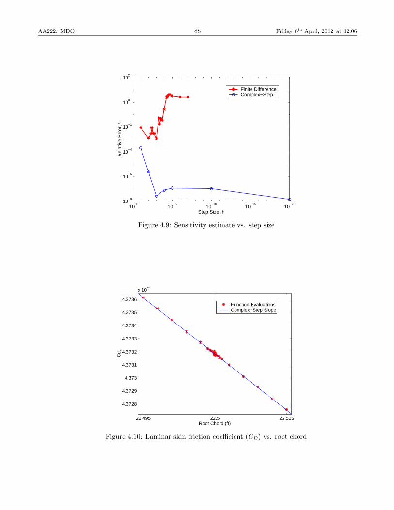
Figure 4.9: Sensitivity estimate vs. step size

22.495 22.5 22.505

4.3728

4.3729

4.373

4.3731

4.3732

4.3733

4.3734

4.3735

4.3736

x 10−4

Root Chord (ft)

Cd f

Function EvaluationsComplex−Step Slope

Figure 4.10: Laminar skin friction coefficient (CD) vs. root chord


When using the forward mode, for each intermediate variable in the algorithm, a variation dueto one input variable is carried through. This is very similar to the way the complex-step methodworks. To illustrate this, suppose we want to differentiate the multiplication operation, f = x1x2,with respect to x1. Table 4.1 compares how the differentiation would be performed using eitherautomatic differentiation or the complex-step method.

Automatic Complex-Step

∆x1 = 1 h1 = 10−20

∆x2 = 0 h2 = 0f = x1x2 f = (x1 + ih1)(x2 + ih2)∆f = x1∆x2 + x2∆x1 f = x1x2 − h1h2 + i(x1h2 + x2h1)df/dx1 = ∆f df/dx1 = Im f/h

Table 4.1: The differentiation of the multiplication operation f = x1x2 with respect to x1 usingautomatic differentiation and the complex-step derivative approximation.

As we can see, automatic differentiation stores the derivative value in a separate set of variableswhile the complex step carries the derivative information in the imaginary part of the variables.It is shown that in this case, the complex-step method performs one additional operation — thecalculation of the term h1h2 — which, for the purposes of calculating the derivative is superfluous(and equals zero in this particular case). The complex-step method will nearly always includethese unnecessary computations which correspond to the higher order terms in the Taylor seriesexpansion. For very small h, when using finite precision arithmetic, these terms have no effect onthe real part of the result.

Although this example involves only one operation, both methods work for an algorithm in-volving an arbitrary sequence of operations by propagating the variation of one input forwardthroughout the code. This means that in order to calculate n derivatives, the differentiated codemust be executed n times.

In general, any program can be written as a sequence of m elementary functions Ti for i =1, . . . ,m, where Ti is a function only of variables t1, . . . , ti−1, and

ti = Ti(t1, . . . , ti−1) (4.27)

The chain rule for composite functions can be applied to each of these operations and is writtenas

∂ti∂tj

= δij +

i−1∑k=j

∂Ti∂tk

∂tk∂tj

, for j ≤ i ≤ n (4.28)

where δij = 1 if i = j, or δij = 0 otherwise. Using the forward mode, we chose one j and keep itfixed. We then work our way forward in the index i = 1, 2, . . . ,m until we get the desired derivative.

The reverse mode, on the other hand, works by fixing i, the desired quantity we want todifferentiate, and working our way backward in the index j = m,m − 1, . . . , 1 all the way to theindependent variables.

Example 4.13. Forward mode differentiation of a simple function by handThere is nothing like an example, so we will now use the forward mode of the chain rule to

compute the derivatives of the vector function,[f1

f2

]=

[(x1x2 + sinx1)

(3x2

2 + 6)

x1x2 + x22

](4.29)


evaluated at x = [π/4, 2].

The solution can be obtained by hand differentiation,

∂f

∂x=

[(x2 + cosx1)

(3x2

2 + 6)

x1

(3x2

2 + 6)

+ 6x2 (x1x2 + sinx1)x2 x1 + 2x2

](4.30)

This matrix of sensitivities at the specified point is,

∂f

∂x=

[48.73 41.472.00 4.79

](4.31)

However, the point of this example is to show how the chain rule can be systematically appliedin an automated fashion. To illustrate this more clearly, we write the function as a series of unaryand binary computations:

t1 = x1

t2 = x2

t3 = T3(t1) = sin t1

t4 = T4(t1, t2) = t1t2

t5 = T5(t2) = t22

t6 = 3

t7 = T7(t3, t4) = t3 + t4

t8 = T8(t5, t6) = t5t6

t9 = 6

t10 = T10(t8, t9) = t8 + t9

t11 = T11(t7, t10) = t7t10 (= f1)

t12 = T12(t4, t5) = t4 + t5 (= f2)

Thus in this case, m = 12.

Now let’s use the forward mode to compute ∂f1/∂x1 in our example, which is ∂t11/∂t1. Thus,we set j = 1 and keep it fixed, and then vary i = 1, 2, . . . , 11. Note that in the sum in the chain


rule, we only include the k’s for which ∂Ti/∂tk 6= 0.

∂t1∂t1

= 1

∂t2∂t1

= 0

∂t3∂t1

=∂T3

∂t1

∂t1∂t1

= cos t1 × 1 = cos t1

∂t4∂t1

=∂T4

∂t1

∂t1∂t1

+∂T4

∂t2

∂t2∂t1

= t2 × 1 + t1 × 0 = t2

∂t5∂t1

=∂T5

∂t2

∂t2∂t1

= 2t2 × 0 = 0

∂t6∂t1

= 0

∂t7∂t1

=∂T7

∂t3

∂t3∂t1

+∂T7

∂t4

∂t4∂t1

= 1× cos t1 + 1× t2 = cos t1 + t2

∂t8∂t1

=∂T8

∂t5

∂t5∂t1

+∂T8

∂t6

∂t6∂t1

= t6 × 0 + t5 × 0 = 0

∂t9∂t1

= 0

∂t10

∂t1=∂T10

∂t8

∂t8∂t1

+∂T10

∂t9

∂t9∂t1

= 1× 0 + 1× 0 = 0

∂t11

∂t1=∂T11

∂t7

∂t7∂t1

+∂T11

∂t10

∂t10

∂t1= t10 (cos t1 + t2) + t7 × 0 =

(3t22 + 6

)(cos t1 + t2)

Note that although we did not set out to compute ∂t12/∂t1, this can be found with littleadditional cost:

∂t12

∂t1=∂T12

∂t4

∂t4∂t1

+∂T12

∂t5

∂t5∂t1

= 1× t2 + 1× 0 = t2

Example 4.14. Forward mode algorithmic differentiation of a simple subroutine

SUBROUTINE CALCF(x, f)

REAL :: x(2), f(2), t(12)

t(1) = x(1)

t(2) = x(2)

t(3) = SIN(t(1))

t(4) = t(1) * t(2)

t(5) = t(2)**2

t(6) = 3

t(7) = t(3) + t(4)

t(8) = t(5) * t(6)

t(9) = 6

t(10) = t(8) + t(9)

t(11) = t(7) * t(10)

t(12) = t(4) + t(5)

f(1) = t(11)

f(2) = t(12)

END SUBROUTINE CALCF

Figure 4.11: Fortran source code for simple function


SUBROUTINE CALCF_D(x, xd , f, fd)

REAL :: x(2), f(2), t(12)

REAL :: xd(2), fd(2), td(12)

td = 0.0

td(1) = xd(1)

t(1) = x(1)

td(2) = xd(2)

t(2) = x(2)

td(3) = td(1)*COS(t(1))

t(3) = SIN(t(1))

td(4) = td(1)*t(2) + t(1)*td(2)

t(4) = t(1)*t(2)

td(5) = 2*t(2)*td(2)

t(5) = t(2)**2

td(6) = 0.0

t(6) = 3

td(7) = td(3) + td(4)

t(7) = t(3) + t(4)

td(8) = td(5)*t(6) + t(5)*td(6)

t(8) = t(5)*t(6)

td(9) = 0.0

t(9) = 6

td(10) = td(8) + td(9)

t(10) = t(8) + t(9)

td(11) = td(7)*t(10) + t(7)*td(10)

t(11) = t(7)*t(10)

td(12) = td(4) + td(5)

t(12) = t(4) + t(5)

fd(1) = td(11)

f(1) = t(11)

fd(2) = td(12)

f(2) = t(12)

END SUBROUTINE CALCF_D

Figure 4.12: Fortran source code for simple function differentiated in forward mode using sourcecode transformation


In the real world, you would not code this way, instead, you would use two lines of code, asshown in Fig. 4.13.

SUBROUTINE CALCF2(x, f)

REAL :: x(2), f(2)

f(1) = (x(1)*x(2) + SIN(x(1))) * (3*x(2)**2 + 6)

f(2) = x(1)*x(2) + x(2)**2

END SUBROUTINE CALCF2

Figure 4.13: Fortran source code for simple function

SUBROUTINE CALCF2_D(x, xd , f, fd)

REAL :: x(2), f(2)

REAL :: xd(2), fd(2)

fd(1) = (xd(1)*x(2)+x(1)*xd(2)+xd(1)*COS(x(1)))*(3*x(2) **2+6) + (x(1)*&

& x(2)+SIN(x(1)))*3*2*x(2)*xd(2)

f(1) = (x(1)*x(2)+SIN(x(1)))*(3*x(2) **2+6)

fd(2) = xd(1)*x(2) + x(1)*xd(2) + 2*x(2)*xd(2)

f(2) = x(1)*x(2) + x(2)**2

END SUBROUTINE CALCF2_D

Figure 4.14: Fortran source code for simple function differentiated in forward mode using sourcecode transformation

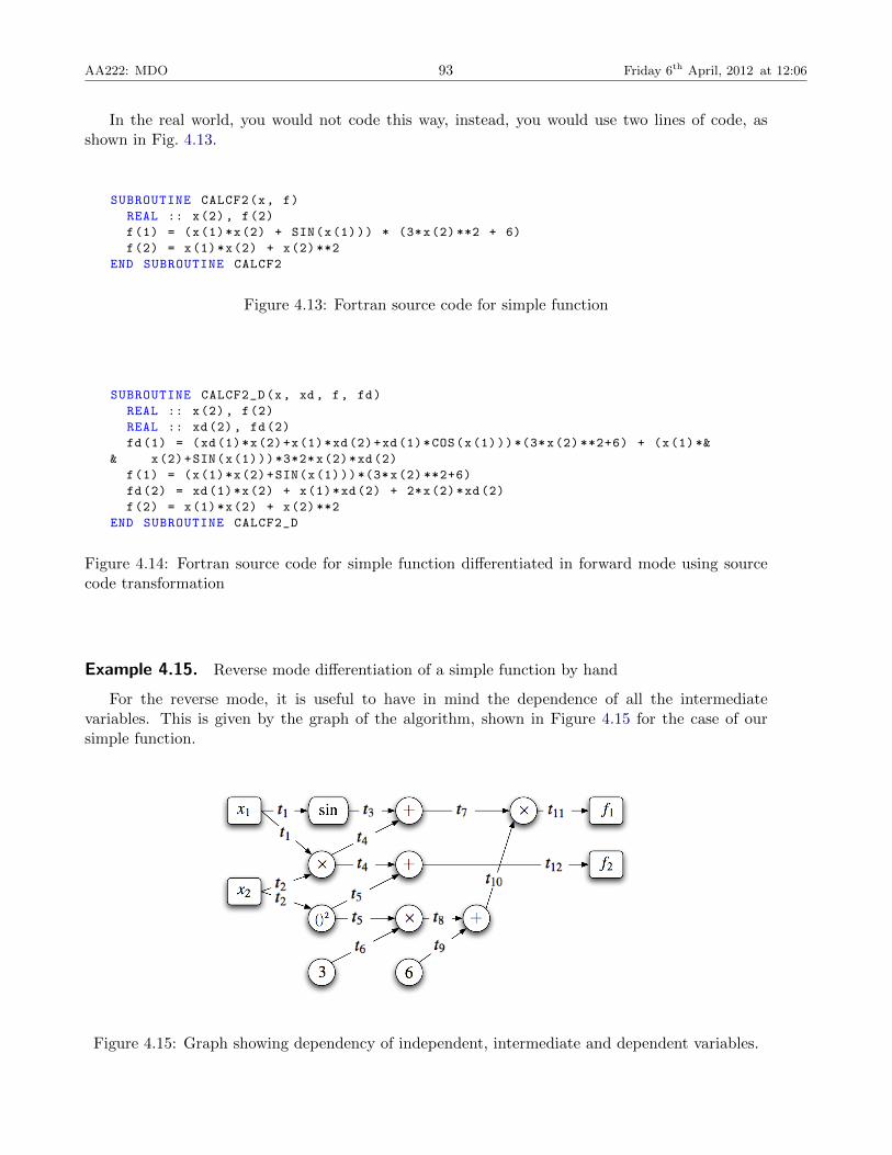
Example 4.15. Reverse mode differentiation of a simple function by hand

For the reverse mode, it is useful to have in mind the dependence of all the intermediatevariables. This is given by the graph of the algorithm, shown in Figure 4.15 for the case of oursimple function.

Figure 4.15: Graph showing dependency of independent, intermediate and dependent variables.


To use the chain rule in reverse, we set i = 11 and loop j = 11, 10, . . . , 1:

∂t11

∂t11= 1

∂t11

∂t10=∂T11

∂t10

∂t10

∂t10= t7 × 1 = t7

∂t11

∂t9=∂T11

∂t9

∂t9∂t9

+∂T11

∂t10

∂t10

∂t9= 0× 1 + t7 × 1 = t7

∂t11

∂t8=∂T11

∂t8

∂t8∂t8

+∂T11

∂t9

∂t9∂t8

+∂T11

∂t10

∂t10

∂t8= 0× 1 + 0× 0 + t7 × 1 = t7

∂t11

∂t7=∂T11

∂t7

∂t7∂t7

+ . . .+∂T11

∂t10

∂t10

∂t7= t10 × 1 + t7 × 0 = t10

∂t11

∂t6= t5t7

∂t11

∂t5= t7t6

∂t11

∂t4= t10

∂t11

∂t3= t10

∂t11

∂t2= t10t1 + t7t62t2 =

(3t22 + 6

)t1 + 6t2 (sin t1 + t1t2)

∂t11

∂t1= t10 cos t1 + t10t2 =

(3x2

2 + 6)

(cosx1 + x2)

Note that although we didn’t set out to compute ∂t11∂t2, it had to be computed anyway.

The cost of calculating the derivative of one output to many inputs is not proportional to thenumber of input but to the number of outputs. Since when using the reverse mode we need tostore all the intermediate variables as well as the complete graph of the algorithm, the amount ofmemory that is necessary increases dramatically. In the case of three-dimensional iterative solver,the cost of using this mode can be prohibitive.

Example 4.16. Fortran code differentiated in reverse mode using source transformation

Now we explain forward and reverse automatic differentiation using matrix algebra. Recall thechain rule (4.32) that forms the basis for both the forward and reverse modes,

∂ti∂tj

= δij +

i−1∑k=j

∂Ti∂tk

∂tk∂tj

, for j ≤ i ≤ n. (4.32)

The partial derivatives of the elementary functions Ti with respect to ti form the Jacobianmatrix,

DT =∂Ti∂tj

=

0 · · ·∂T2∂t1

0 · · ·∂T3∂t1

∂T3∂t2

0 · · ·...

......

. . .

(4.33)


SUBROUTINE CALCF_B(x, xb , f, fb)

REAL :: x(2), f(2), t(12)

REAL :: xb(2), fb(2), tb(12)

INTRINSIC SIN

t(1) = x(1)

t(2) = x(2)

CALL PUSHREAL4(t(3))

t(3) = SIN(t(1))


t(4) = t(1)*t(2)


t(5) = t(2)**2


t(6) = 3


t(7) = t(3) + t(4)


t(8) = t(5)*t(6)


t(9) = 6


t(10) = t(8) + t(9)

tb = 0.0

tb(12) = tb(12) + fb(2)

fb(2) = 0.0

tb(11) = tb(11) + fb(1)

fb(1) = 0.0

tb(4) = tb(4) + tb(12)

tb(5) = tb(5) + tb(12)

tb(12) = 0.0

tb(7) = tb(7) + t(10)*tb(11)

tb(10) = tb(10) + t(7)*tb(11)

tb(11) = 0.0

CALL POPREAL4(t(10))

tb(8) = tb(8) + tb(10)

tb(9) = tb(9) + tb(10)

tb(10) = 0.0

CALL POPREAL4(t(9))

tb(9) = 0.0

CALL POPREAL4(t(8))

tb(5) = tb(5) + t(6)*tb(8)

tb(6) = tb(6) + t(5)*tb(8)

tb(8) = 0.0

CALL POPREAL4(t(7))

tb(3) = tb(3) + tb(7)

tb(4) = tb(4) + tb(7)

tb(7) = 0.0

CALL POPREAL4(t(6))

tb(6) = 0.0

CALL POPREAL4(t(5))

tb(2) = tb(2) + 2*t(2)*tb(5)

tb(5) = 0.0

CALL POPREAL4(t(4))

tb(1) = tb(1) + t(2)*tb(4)

tb(2) = tb(2) + t(1)*tb(4)

tb(4) = 0.0

CALL POPREAL4(t(3))

tb(1) = tb(1) + COS(t(1))*tb(3)

tb(3) = 0.0

xb = 0.0

xb(2) = xb(2) + tb(2)

tb(2) = 0.0

xb(1) = xb(1) + tb(1)

END SUBROUTINE CALCF_B

Figure 4.16: Fortran source code for simple function differentiated in reverse mode using sourcecode transformation


SUBROUTINE CALCF2_B(x, xb , f, fb)

IMPLICIT NONE

REAL :: x(2), f(2)

REAL :: xb(2), fb(2)

INTRINSIC SIN

REAL :: tempb

xb = 0.0

xb(1) = xb(1) + x(2)*fb(2)

xb(2) = xb(2) + (2*x(2)+x(1))*fb(2)

fb(2) = 0.0

tempb = (3*x(2) **2+6)*fb(1)

xb(1) = xb(1) + (COS(x(1))+x(2))*tempb

xb(2) = xb(2) + 3*(x(1)*x(2)+SIN(x(1)))*2*x(2)*fb(1) + x(1)*tempb

fb(1) = 0.0

END SUBROUTINE CALCF2_B

Figure 4.17: Fortran source code for simple function differentiated in reverse mode using sourcecode transformation

The total derivatives of the variables ti form another matrix,

Dt =∂ti∂tj

=

1 0 · · ·∂t2∂t1

1 0 · · ·∂t3∂t1

∂t3∂t2

1 0...

......

. . .

(4.34)

This can be written as a matrix equation,

Dt = I + DTDt ⇔(I−DT) Dt = I ⇔ (4.35)

Dt = (I−DT)−1 ⇔Dt (I−DT) = I ⇔

(I−DT)T DtT = I (4.36)

Example 4.17. Simple function differentiation in matrix formIn our example, this matrix equation is,

1 0 0 0 0 0 0 0 0 0 0 0

0 1 0 0 0 0 0 0 0 0 0 0

−√2/2 0 1 0 0 0 0 0 0 0 0 0

−2 −π/4 0 1 0 0 0 0 0 0 0 0

0 −4 0 0 1 0 0 0 0 0 0 0

0 0 0 0 0 1 0 0 0 0 0 0

0 0 −1 −1 0 0 1 0 0 0 0 0

0 0 0 0 −3 −4 0 1 0 0 0 0

0 0 0 0 0 0 0 0 1 0 0 0

0 0 0 0 0 0 0 −1 −1 1 0 0

0 0 0 0 0 0 −18 0 0 −2.28 1 0

0 0 0 −1 −1 0 0 0 0 0 0 1

∂t1∂x1

∂t1∂x2

∂t2∂x1

∂t2∂x2

∂t3∂x1

∂t3∂x2

.

.

.

.

.

.∂t9∂x1

∂t9∂x2

∂t10∂x1

∂t10∂x2

∂f1∂x1

∂f1∂x2

∂f2∂x1

∂f2∂x2

=

1 0

0 1

0 0

0 0

0 0

0 0

0 0

0 0

0 0

0 0

0 0

0 0

(4.37)


The solution of this system is

∂t1∂x1

∂t1∂x2

∂t2∂x1

∂t2∂x2

∂t3∂x1

∂t3∂x2

.

.

.

.

.

.∂t10∂x1

∂t10∂x2

∂f1∂x1

∂f1∂x2

∂f2∂x1

∂f2∂x2

=

1 00 1

0.71 02 0.790 40 0

2.71 0.790 120 00 12

48.73 41.472 4.79

(4.38)

4.5.2 Tools for Algorithmic Differentiation

There are two main methods for implementing automatic differentiation: by source code transfor-mation or by using derived datatypes and operator overloading.

To implement automatic differentiation by source transformation, the whole source code mustbe processed with a parser and all the derivative calculations are introduced as additional lines ofcode. The resulting source code is greatly enlarged and it becomes practically unreadable. Thisfact might constitute an implementation disadvantage as it becomes impractical to debug this newextended code. One has to work with the original source, and every time it is changed (or if differentderivatives are desired) one must rerun the parser before compiling a new version. The advantageis that this method tends to yield faster code.

In order to use derived types, we need languages that support this feature, such as Fortran 90 orC++. To implement automatic differentiation using this feature, a new type of structure is createdthat contains both the value and its derivative. All the existing operators are then re-defined(overloaded) for the new type. The new operator has exactly the same behavior as before for thevalue part of the new type, but uses the definition of the derivative of the operator to calculatethe derivative portion. This results in a very elegant implementation since very few changes arerequired in the original code.

There are automatic differentiation tools available for a variety of programming languages in-cluding Fortran, C/C++ and Matlab. They have been extensively developed and provide the userwith great functionality, including the calculation of higher-order derivatives and reverse modeoptions.

Fortran

ADIFOR [6], TAF [8], TAMC [9], DAFOR, GRESS and Tapenade [11, 19] are some of the toolsavailable for Fortran that use source transformation. The necessary changes to the source code aremade automatically. The derived datatype approach is used in the following tools: AD01, ADOL-F, IMAS and OPTIMA90. Although it is in theory possible to have a script make the necessarychanges in the source code automatically, none of these tools have this facility and the changesmust be done manually.

C/C++:

Established tools for automatic differentiation also exist for C/C++. These include include ADIC,an implementation mirroring ADIFOR, and ADOL-C, a free package that uses operator overloadingand can operate in the forward or reverse modes and compute higher order derivatives.


4.5.3 The Connection to Algorithmic Differentiation

The new function definitions in these examples can be generalized:

f(x+ ih) ≡ f(x) + ih∂f(x)

∂x. (4.39)

The real part is the real function and the imaginary part is the derivative multiplied by h.Defining functions this way, or for small enough step using finite precision arithmetic, the complex-step method is the same as automatic differentiation.

Looking at a simple operation, e.g. f = x1x2,

Algorithmic Complex-Step

∆x1 = 1 h1 = 10−20

∆x2 = 0 h2 = 0f = x1x2 f = (x1 + ih1)(x2 + ih2)∆f = x1∆x2 + x2∆x1 f = x1x2−h1h2 + i(x1h2 + x2h1)df/dx1 = ∆f df/dx1 = Im f/h

Complex-step method computes one extra term. Other functions are similar:

• Superfluous calculations are made.

• For h ≤ x× 10−20 they vanish but still affect speed.

Example 4.18. Complex-step method example Consider a more involved function, e.g., f =(xy + sinx+ 4)(3y2 + 6),

t1 = x+ ih, t2 = y

t3 = xy + iyh

t4 = sinx coshh+ icosx sinhh

t5 = xy + sinx coshh+ i(yh+ cosx sinhh)

t6 = xy + sinx coshh+ 4 + i(yh+ cosx sinhh)

t7 = y2, t8 = 3y2, t9 = 3y2 + 6

t10 = (xy + sinx coshh+ 4)(3y2 + 6

)+ i(yh+ cosx sinhh)

(3y2 + 6

)df

dx≈ Im [f(x+ ih, y)]

h=

(y + cosx

sinhh

h

)(3y2 + 6

)Large body of research on automatic differentiation can now be applied to the complex-step

method:

• Singularities: non-analytic points

• if statements: piecewise function definitions

• Convergence for iterative solvers

• Other issues addressed by the automatic differentiation community


4.5.4 Algorithmic Differentiation vs. Complex Step

• Algorithmic Differentiation

– Source transformation (ADIFOR, ADIC):resulting code is unmaintainable.

– Derived datatype and operator overloading (ADOL-F, ADOL-C):far fewer changes are necessary in source code, requires object-oriented language.

• Complex Step:

– Even fewer changes are required.

– Resulting code is maintainable.

– Can be easily implemented in any programming language that supports complex arith-metic.

4.6 Analytic Sensitivity Analysis

Analytic methods are the most accurate and efficient methods available for sensitivity analysis.They are, however, more involved than the other methods we have seen so far since they requirethe knowledge of the governing equations and the algorithm that is used to solve those equations.In this section we will learn how to compute analytic sensitivities with direct and adjoint methods.We will start with single discipline systems and then generalize for the case of multiple systemssuch as we would encounter in MDO.

4.6.1 Notation

f function of interest/output (could be a vector)Rk residuals of governing equation, k = 1, . . . , NRxn design/independent/input variables, n = 1, . . . , Nx

yi state variables, i = 1, . . . , NRΨk adjoint vector, k = 1, . . . , NR

4.6.2 Basic Equations

The main objective is to calculate the sensitivity of a multidisciplinary function of interest withrespect to a number of design variables. The function of interest can be either the objective functionor any of the constraints specified in the optimization problem. In general, such functions dependnot only on the design variables, but also on the physical state of the multidisciplinary system.Thus we can write the function as

f = f(xn, yi), (4.40)

where xn represents the vector of design variables and yi is the state variable vector.For a given vector xn, the solution of the governing equations of the multidisciplinary system

yields a vector yi, thus establishing the dependence of the state of the system on the design variables.We denote these governing equations by

Rk (xn, yi (xn)) = 0. (4.41)

The first instance of xn in the above equation indicates the fact that the residual of the governingequations may depend explicitly on xn. In the case of a structural solver, for example, changing the


size of an element has a direct effect on the stiffness matrix. By solving the governing equationswe determine the state, yi, which depends implicitly on the design variables through the solutionof the system. These equations may be non-linear, in which case the usual procedure is to driveresiduals, Rk, to zero using an iterative method.

Since the number of equations must equal the number of state variables, the ranges of theindices i and k are the same, i.e., i, k = 1, . . . , NR. In the case of a structural solver, for example,NR is the number of degrees of freedom, while for a CFD solver, NR is the number of meshpoints multiplied by the number of state variables at each point. In the more general case ofa multidisciplinary system, Rk represents all the governing equations of the different disciplines,including their coupling.

� �

� �

�

Figure 4.18: Schematic representation of the governing equations (Rk = 0), design variables orinputs (xj), state variables (yi) and the function of interest or output (f).

A graphical representation of the system of governing equations is shown in Figure 4.18, withthe design variables xn as the inputs and f as the output. The two arrows leading to f illustratethe fact that the objective function typically depends on the state variables and may also be anexplicit function of the design variables.

As a first step toward obtaining the derivatives that we ultimately want to compute, we use thechain rule to write the total sensitivity of f as

df

dxn=

∂f

∂xn+∂f

∂yi

dyidxn

, (4.42)

for i = 1, . . . , NR, n = 1, . . . , Nx. Index notation is used to denote the vector dot products. It isimportant to distinguish the total and partial derivatives in this equation. The partial derivativescan be directly evaluated by varying the denominator and re-evaluating the function in the numer-ator. The total derivatives, however, require the solution of the multidisciplinary problem. Thus,all the terms in the total sensitivity equation (4.42) are easily computed except for dyi/ dxn.

Since the governing equations must always be satisfied, the total derivative of the residuals (4.41)with respect to any design variable must also be zero. Expanding the total derivative of thegoverning equations with respect to the design variables we can write,

dRkdxn

=∂Rk∂xn

+∂Rk∂yi

dyidxn

= 0, (4.43)

for all i, k = 1, . . . , NR and n = 1, . . . , Nx. This expression provides the means for computingthe total sensitivity of the state variables with respect to the design variables. By rewriting equa-tion (4.43) as

∂Rk∂yi

dyidxn

= −∂Rk∂xn

. (4.44)


We can solve for dyi/ dxn and substitute this result into the total derivative equation (4.42),to obtain

df

dxn=

∂f

∂xn− ∂f

∂yi

− dyi/dxn︷︸︸︷[∂Rk∂yi

]−1 ∂Rk∂xn

.︸︷︷︸Ψk

(4.45)

The inverse of the Jacobian ∂Rk/∂yi is not necessarily explicitly calculated. In the case of largeiterative problems neither this matrix nor its factorization are usually stored due to their prohibitivesize.

4.6.3 Direct Sensitivity Equations

The approach where we first calculate dyi/ dxn using equation (4.44) and then substitute the resultin the expression for the total sensitivity (4.45) is called the direct method. Note that solving fordyi/dxn requires the solution of the matrix equation (4.44) for each design variable xn. A changein the design variable affects only the right-hand side of the equation, so for problems where thematrix ∂Rk/∂yi can be explicitly factorized and stored, solving for multiple right-hand-side vectorsby back substitution would be relatively inexpensive. However, for large iterative problems —such as the ones encountered in CFD — the matrix ∂Rk/∂yi is never factorized explicitly andthe system of equations requires an iterative solution which is usually as costly as solving thegoverning equations. When we multiply this cost by the number of design variables, the total costfor calculating the sensitivity vector may become unacceptable.

4.6.4 Adjoint Sensitivity Equations

Returning to the total sensitivity equation (4.45), we observe that there is an alternative optionfor computing the total sensitivity df/dxn. The auxiliary vector Ψk can be obtained by solvingthe adjoint equations

∂Rk∂yi

Ψk = − ∂f∂yi

. (4.46)

The vector Ψk is usually called the adjoint vector and is substituted into equation (4.45) to findthe total sensitivity. In contrast with the direct method, the adjoint vector does not depend on thedesign variables, xn, but instead depends on the function of interest, f .

4.6.5 Direct vs. Adjoint

We can now see that the choice of the solution procedure (direct vs. adjoint) to obtain the totalsensitivity (4.45) has a substantial impact on the cost of sensitivity analysis. Although all thepartial derivative terms are the same for both the direct and adjoint methods, the order of theoperations is not. Notice that once dyi/ dxn is computed, it is valid for any function f , but mustbe recomputed for each design variable (direct method). On the other hand, Ψk is valid for alldesign variables, but must be recomputed for each function (adjoint method).

The cost involved in calculating sensitivities using the adjoint method is therefore practicallyindependent of the number of design variables. After having solved the governing equations, theadjoint equations are solved only once for each f . Moreover, the cost of solution of the adjointequations is similar to that of the solution of the governing equations since they are of similarcomplexity and the partial derivative terms are easily computed.


Step Direct Adjoint

Factorization same same

Back-solve Nx times Nf times

Multiplication same same

Therefore, if the number of design variables is greater than the number of functions for whichwe seek sensitivity information, the adjoint method is computationally more efficient. Otherwise,if the number of functions to be differentiated is greater than the number of design variables, thedirect method would be a better choice.

A comparison of the cost of computing sensitivities with the direct versus adjoint methods isshown in Table ??. With either method, we must factorize the same matrix, ∂Rk/∂yi. The differ-ence in the cost comes form the back-solve step for solving equations (4.44) and (4.59) respectively.The direct method requires that we perform this step for each design variable (i.e. for each j)while the adjoint method requires this to be done for each function of interest (i.e. for each i). Themultiplication step is simply the calculation of the final sensitivity expressed in equations (4.44)and (4.59) respectively. The cost involved in this step when computing the same set of sensitivitiesis the same for both methods.

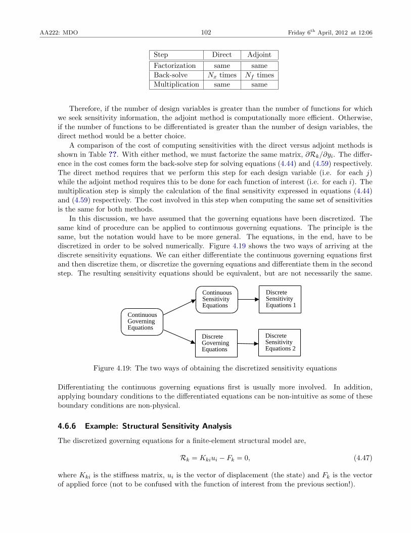
In this discussion, we have assumed that the governing equations have been discretized. Thesame kind of procedure can be applied to continuous governing equations. The principle is thesame, but the notation would have to be more general. The equations, in the end, have to bediscretized in order to be solved numerically. Figure 4.19 shows the two ways of arriving at thediscrete sensitivity equations. We can either differentiate the continuous governing equations firstand then discretize them, or discretize the governing equations and differentiate them in the secondstep. The resulting sensitivity equations should be equivalent, but are not necessarily the same.

ContinuousGoverningEquations

ContinuousSensitivityEquations

DiscreteGoverningEquations

DiscreteSensitivityEquations 2

DiscreteSensitivityEquations 1

Figure 4.19: The two ways of obtaining the discretized sensitivity equations

Differentiating the continuous governing equations first is usually more involved. In addition,applying boundary conditions to the differentiated equations can be non-intuitive as some of theseboundary conditions are non-physical.

4.6.6 Example: Structural Sensitivity Analysis

The discretized governing equations for a finite-element structural model are,

Rk = Kkiui − Fk = 0, (4.47)

where Kki is the stiffness matrix, ui is the vector of displacement (the state) and Fk is the vectorof applied force (not to be confused with the function of interest from the previous section!).


We are interested in finding the sensitivities of the stress, which is related to the displacementsby the equation,

σm = Smiui. (4.48)

We will consider the design variables to be the cross-sectional areas of the elements, Aj . We willnow look at the terms that we need to use the generalized total sensitivity equation (4.45).

For the matrix of sensitivities of the governing equations with respect to the state variables wefind that it is simply the stiffness matrix, i.e.,

∂Rk∂yi

=∂(Kkiui − Fk)

∂ui= Kki. (4.49)

Let’s consider the sensitivity of the residuals with respect to the design variables (cross-sectionalareas in our case). Neither the displacements of the applied forces vary explicitly with the elementsizes. The only term that depends on Aj directly is the stiffness matrix, so we get,

∂Rk∂xj

=∂(Kkiui − Fk)

∂Aj=∂Kki

∂Ajui (4.50)

The partial derivative of the stress with respect to the displacements is simply given by the matrixin equation (4.48), i.e.,

∂fm∂yi

=∂σm∂ui

= Smi (4.51)

Finally, the explicit variation of stress with respect to the cross-sectional areas is zero, since thestresses depends only on the displacement field,

∂fm∂xj

=∂σm∂Aj

= 0. (4.52)

Substituting these into the generalized total sensitivity equation (4.45) we get:

dσmdAj

= −∂σm∂ui

K−1ki

∂Kki

∂Ajui (4.53)

Referring to the theory presented previously, if we were to use the direct method, we would solve,

KkiduidAj

= −∂Kki

∂Ajui (4.54)

and then substitute the result in,dσmdAj

=∂σm∂ui

duidAj

(4.55)

to calculate the desired sensitivities.The adjoint method could also be used, in which case we would solve equation (4.59) for the

structures case,

KTkiψk =

∂σm∂ui

. (4.56)

Then we would substitute the adjoint vector into the equation,

dσmdAj

=∂σm∂Aj

+ ψTk

(−∂Kki

∂Ajui

). (4.57)

to calculate the desired sensitivities.

Example 4.19. Computational Accuracy and Cost


Method Sample Sensitivity Time Memory

Complex –39.049760045804646 1.00 1.00

ADIFOR –39.049760045809059 2.33 8.09

Analytic –39.049760045805281 0.58 2.42

FD –39.049724352820375 0.88 0.72

• All except finite-difference achieve thesolver’s precision.

• Analytic: best, but not easy to implement.

• ADIFOR: costly.

• Complex-step: good compromise.

• Caveat: ratios depend on problem.

Example 4.20. The Automatic Differentiation Adjoint (ADjoint) Method [? ]The automatic differentiation adjoint (ADjoint) method is a hybrid between automatic differ-

entiation and the adjoint method. In a nutshell, we take the adjoint equations formulated above,compute the partial derivatives in those equations with automatic differentiation, and then solvethe linear system and perform the necessary matrix-vector products.

We chose to use Tapenade as it is the only non-commercial tool with support for Fortran90. Tapenade is the successor of Odyssee [7] and was developed at the INRIA. It uses sourcetransformation and can perform differentiation in either forward or reverse mode. Furthermore,the Tapenade team is actively developing their software and has been very responsive to a numberof suggestions towards completing their support of the Fortran 90 standard.

In order to verify the results given by the ADjoint approach we decided to use the complex-stepderivative approximation [13, 15] as our benchmark.

In semi-discrete form the Euler equations are,

dwijkdt

+Rijk(w) = 0, (4.58)

where R is the residual described earlier with all of its components (fluxes, boundary conditions,artificial dissipation, etc.).

The adjoint equations (??) can be re-written for this flow solver as,[∂R∂w

]Tψ = − ∂I

∂w. (4.59)

where ψ is the adjoint vector. The total sensitivity (4.42) in this case is,

dI

dx=∂I

∂x+ ψT

∂R∂x

. (4.60)

We propose to compute the partial derivative matrices ∂R/∂w, ∂I/∂w, ∂I/∂x and ∂R/∂xusing automatic differentiation instead of using manual differentiation or using finite differences.Where appropriate we will use the reverse mode of automatic differentiation.

To better understand the choices made in the mode of differentiation as well as the effect ofthese choices in the general case we define the following numbers:


−3 −2 −1 0 1 2 3 −2−1

01

2−2.5

−2

−1.5

−1

−0.5

0

0.5

1

1.5

2

2.5

ji

k

Figure 4.20: Stencil for the residual computation

SUBROUTINE RESIDUAL(w, r, ni, nj)

IMPLICIT NONE

INTEGER :: ni , nj

REAL :: r(ni, nj), w(0:ni+1, 0:nj+1)

INTEGER :: i, j

INTRINSIC SQRT

DO i=1,ni

DO j=1,nj

w(i, j) = w(i, j) + SQRT(w(i, j-1)*w(i, j+1))

r(i, j) = w(i, j)*w(i-1, j) + SQRT(w(i+1, j)) + &

& w(i, j-1)*w(i, j+1)

END DO

END DO

END SUBROUTINE RESIDUAL

Figure 4.21: Simplified subroutine for residual calculation

Nc: The number of cells in the domain. For three-dimensional domains where the Navier–Stokesequations are solved, this can be O(106).

Ns: The number of cells in the stencil whose variables affect the residual of a given cell. In ourcase, we consider inviscid and dissipation fluxes, so the stencil is as shown in Figure 4.20 andNs = 13.

Nw: The number of flow variables (and also residuals) for each cell. In our case Nw = 5.

In principle, because ∂R/∂w is a square matrix, neither mode should have an advantage over theother in terms of computational time. However, due to the way residuals are computed, the reversemode is much more efficient. To explain the reason for this, consider a very simplified version of acalculation resembling the residual calculation in CFD shown in Figure 4.21. This subroutine loopsthrough a two-dimensional domain and computes r (the “residual”) in the interior of that domain.The residual at any cell depends only on the ws (the “flow variables”) at that cell and at the cellsimmediately adjacent to it, thus the stencil of dependence forms a cross with five cells.


SUBROUTINE RESIDUAL_D(w, wd, r, rd, ni, nj)

IMPLICIT NONE

INTEGER :: ni , nj

REAL :: r(ni, nj), rd(ni, nj)

REAL :: w(0:ni+1, 0:nj+1), wd(0:ni+1, 0:nj+1)

INTEGER :: i, j

REAL :: arg1 , arg1d , result1 , result1d

INTRINSIC SQRT

rd(1:ni , 1:nj) = 0.0

DO i=1,ni

DO j=1,nj

arg1d = wd(i, j-1)*w(i, j+1) + w(i, j-1)*wd(i, j+1)

arg1 = w(i, j-1)*w(i, j+1)

IF (arg1d .EQ. 0.0 .OR. arg1 .EQ. 0.0) THEN

result1d = 0.0

ELSE

result1d = arg1d /(2.0* SQRT(arg1))

END IF

result1 = SQRT(arg1)

wd(i, j) = wd(i, j) + result1d

w(i, j) = w(i, j) + result1

IF (wd(i+1, j) .EQ. 0.0 .OR. w(i+1, j) .EQ. 0.0) THEN

result1d = 0.0

ELSE

result1d = wd(i+1, j)/(2.0* SQRT(w(i+1, j)))

END IF

result1 = SQRT(w(i+1, j))

rd(i, j) = wd(i, j)*w(i-1, j) + w(i, j)*wd(i-1, j) + &

& result1d + wd(i, j-1)*w(i, j+1) + &

& w(i, j-1)*wd(i, j+1)

r(i, j) = w(i, j)*w(i-1, j) + result1 + &

& w(i, j-1)*w(i, j+1)

END DO

END DO

END SUBROUTINE RESIDUAL_D

Figure 4.22: Subroutine differentiated using the forward mode

The residual computation in our three-dimensional CFD solver is obviously much more compli-cated: It involves multiple subroutines, a larger stencil, the computation of the different fluxes andapplies many different types of boundary conditions. However, this simple example is sufficient todemonstrate the computational inefficiencies of a purely automatic approach.

Forward mode differentiation was used to produce the subroutine shown in Figure 4.22. Twonew variables are introduced: wd, which is the seed vector and rd, which is the gradient of all rs inthe direction specified by the seed vector. For example, if we want the derivative with respect tow(1,1), we would set wd(1,1)=1 and all other wds to zero. One can only choose one direction ata time, although Tapenade can be run in “vectorial” mode to get the whole vector of sensitivities.In this case, an additional loop inside the nested loop and additional storage are required. For ourpurposes, the differentiated code would have to be called Nc ×Nw times.

The subroutine produced by reverse mode differentiation is shown in Figure 4.23. This caseshows the additional storage requirements: Since the ws are overwritten, the old values must bestored for later use in the reversed loop.

The overwriting of the flow variables in the first nested loops of the original subroutine ischaracteristic of iterative solvers. Whenever overwriting is present, the reverse mode needs tostore the time history of the intermediate variables. Tapenade provides functions (PUSHREAL andPOPREAL) to do this. In this case, we can see that the ws are stored before they are modified in the


SUBROUTINE RESIDUAL_B(w, wb, r, rb, ni, nj)

IMPLICIT NONE

INTEGER :: ni , nj

REAL :: r(ni, nj), rb(ni , nj)

REAL :: w(0:ni+1, 0:nj+1), wb(0:ni+1, 0:nj+1)

INTEGER :: i, j

REAL :: tempb

INTRINSIC SQRT

DO i=1,ni

DO j=1,nj

CALL PUSHREAL4(w(i, j))

w(i, j) = w(i, j) + SQRT(w(i, j-1)*w(i, j+1))

END DO

END DO

wb(0:ni+1, 0:nj+1) = 0.0

DO i=ni ,1,-1

DO j=nj ,1,-1

wb(i, j) = wb(i, j) + w(i-1, j)*rb(i, j)

wb(i-1, j) = wb(i-1, j) + w(i, j)*rb(i, j)

wb(i+1, j) = wb(i+1, j) + rb(i, j)/(2.0* SQRT(w(i+1, j)))

wb(i, j-1) = wb(i, j-1) + w(i, j+1)*rb(i, j)

wb(i, j+1) = wb(i, j+1) + w(i, j-1)*rb(i, j)

rb(i, j) = 0.0

CALL POPREAL4(w(i, j))

tempb = wb(i, j)/(2.0* SQRT(w(i, j-1)*w(i, j+1)))

wb(i, j-1) = wb(i, j-1) + w(i, j+1)*tempb

wb(i, j+1) = wb(i, j+1) + w(i, j-1)*tempb

END DO

END DO

END SUBROUTINE RESIDUAL_B

Figure 4.23: Subroutine differentiated using the reverse mode

forward sweep, and then retrieved in the reverse sweep.

On this basis, reverse mode was used to produce adjoint code for this set of routines. Thecall graph for the original and the differentiated routines are shown in Figures 4.24 and 4.25,respectively.

The test case is the Lockheed-Air Force-NASA-NLR (LANN) wing [21], which is a supercriticaltransonic transport wing. A symmetry boundary condition is used at the root and a linear pressureextrapolation boundary condition is used on the wing surface. The freestream Mach number is0.621.

The meshes for this test case is shown in Figure ??.

In Table 4.2 we show the sensitivities of both drag and lift coefficients with respect to freestreamMach number for different cases. The wing mesh and the fine mesh cases are the two test casesdescribed earlier (Figures ?? and ??). The “coarse” case is a very small mesh (12× 4× 4) with thesame geometry as the fine bump case.

We can see that the adjoint sensitivities for these cases are extremely accurate, yielding betweentwelve and fourteen digits agreement when compared to the complex-step results. This is consistentwith the convergence tolerance that was specified in PETSc for the adjoint solution.

To analyze the performance of the ADjoint solver, several timings were performed. They areshown in Table 4.3 for the three cases mentioned above. The coarse grid has 5, 120 flow variables,the fine grid has 203, 840 flow variables and the wing grid has 108, 800 flow variables.

The total cost of the adjoint solver, including the computation of all the partial derivatives andthe solution of the adjoint system, is less than one fourth the cost of the flow solution for the finebump case and less that one eighth the cost of the flow solution for the wing case. This is even


Figure 4.24: Original residual calculation

Figure 4.25: Differentiated residual calculation


Figure 4.26: Wing mesh and density distribution


Table 4.2: Sensitivities of drag and lift coefficients with respect to M∞

Mesh Coefficient Inflow direction ADjoint Complex step

Coarse CD (1,0,0) -0.289896632731764 -0.289896632731759CL -0.267704455366714 -0.267704455366683

Fine CD (1,0,0) -0.0279501183024705 -0.0279501183024709CL 0.58128604734707 0.58128604734708

Coarse CD (1,0.05,0) -0.278907645833786 -0.278907645833792CL -0.262086315233911 -0.262086315233875

Fine CD (1,0.05,0) -0.0615598631060438 -0.0615598631060444CL -0.364796754652787 -0.364796754652797

Wing CD ( 1, 0.0102,0) 0.00942875710535217 0.00942875710535312CL 0.26788212595474 0.26788212595468

better than what is usually observed in the case of adjoint solvers developed by conventional means,showing that the ADjoint approach is indeed very efficient.

Table 4.3: ADjoint computational cost breakdown (times in seconds)

Fine Wing

Flow solution 219.215 182.653

ADjoint 51.959 20.843Breakdown:Setup PETSc variables 0.011 0.004Compute flux Jacobian 11.695 5.870Compute RHS 8.487 2.232Solve the adjoint equations 28.756 11.213Compute the total sensitivity 3.010 1.523


Bibliography

[1] Tools for automatic differentiation. URL http://www.sc.rwth-aachen.de/Research/AD/

subject.html.

[2] Thomas Beck. Automatic differentiation of iterative processes. Journal of Computational andApplied Mathematics, 50:109–118, 1994.

[3] Thomas Beck and Herbert Fischer. The if-problem in automatic differentiation. Journal ofComputational and Applied Mathematics, 50:119–131, 1994.

[4] Claus Bendtsen and Ole Stauning. FADBAD, a flexible C++ package for automatic differ-entiation — using the forward and backward methods. Technical Report IMM-REP-1996-17,Technical University of Denmark, DK-2800 Lyngby, Denmark, 1996. URL citeseer.nj.nec.

com/bendtsen96fadbad.html.

[5] C. H. Bischof, L. Roh, and A. J. Mauer-Oats. ADIC: an extensible automatic differentia-tion tool for ANSI-C. Software — Practice and Experience, 27(12):1427–1456, 1997. URLciteseer.nj.nec.com/article/bischof97adic.html.

[6] Alan Carle and Mike Fagan. ADIFOR 3.0 overview. Technical Report CAAM-TR-00-02, RiceUniversity, 2000.

[7] C. Faure and Y. Papegay. Odyssee Version 1.6: The Language Reference Manual. INRIA,1997. Rapport Technique 211.

[8] Ralf Giering and Thomas Kaminski. Applying TAF to generate efficient derivative code ofFortran 77-95 programs. In Proceedings of GAMM 2002, Augsburg, Germany, 2002.

[9] Mark S. Gockenbach. Understanding Code Generated by TAMC. IAAA Paper TR00-29,Department of Computational and Applied Mathematics, Rice University, Texas, USA, 2000.URL http://www.math.mtu.edu/~msgocken.

[10] Andreas Griewank. Evaluating Derivatives. SIAM, Philadelphia, 2000.

[11] L. Hascoet and V Pascual. Tapenade 2.1 user’s guide. Technical report 300, INRIA, 2004.URL http://www.inria.fr/rrrt/rt-0300.html.

[12] J. N. Lyness. Numerical algorithms based on the theory of complex variable. In Proceedings— ACM National Meeting, pages 125–133, Washington DC, 1967. Thompson Book Co.

[13] J. N. Lyness and C. B. Moler. Numerical differentiation of analytic functions. SIAM Journalon Numerical Analysis, 4(2):202–210, 1967. ISSN 0036-1429 (print), 1095-7170 (electronic).

[14] Joaquim R. R. A. Martins. A guide to the complex-step derivative approximation, 2003. URLhttp://mdolab.utias.utoronto.ca/resources/complex-step/.

[15] Joaquim R. R. A. Martins, Peter Sturdza, and Juan J. Alonso. The complex-step derivativeapproximation. ACM Transactions on Mathematical Software, 29(3):245–262, 2003. doi: 10.1145/838250.838251.

[16] Joaquim R. R. A. Martins, Juan J. Alonso, and James J. Reuther. High-fidelity aerostructuraldesign optimization of a supersonic business jet. Journal of Aircraft, 41(3):523–530, 2004. doi:10.2514/1.11478.

http://www.sc.rwth-aachen.de/Research/AD/subject.html

http://www.sc.rwth-aachen.de/Research/AD/subject.html

citeseer.nj.nec.com/bendtsen96fadbad.html

citeseer.nj.nec.com/bendtsen96fadbad.html

citeseer.nj.nec.com/article/bischof97adic.html

http://www.math.mtu.edu/~msgocken

http://www.inria.fr/rrrt/rt-0300.html

http://mdolab.utias.utoronto.ca/resources/complex-step/


[17] Joaquim R. R. A. Martins, Juan J. Alonso, and James J. Reuther. A coupled-adjoint sensitivityanalysis method for high-fidelity aero-structural design. Optimization and Engineering, 6(1):33–62, March 2005. doi: 10.1023/B:OPTE.0000048536.47956.62.

[18] Siva Nadarajah and Antony Jameson. A comparison of the continuous and discrete adjointapproach to automatic aerodynamic optimization. In Proceedings of the 38th AIAA AerospaceSciences Meeting and Exhibit, Reno, NV, 2000. AIAA 2000-0667.

[19] V. Pascual and L. Hascoet. Extension of TAPENADE towards Fortran 95. In H. M. Bucker,G. Corliss, P. Hovland, U. Naumann, and B. Norris, editors, Automatic Differentiation: Appli-cations, Theory, and Tools, Lecture Notes in Computational Science and Engineering. Springer,2005.

[20] John D. Pryce and John K. Reid. AD01, a Fortran 90 code for automatic differentiation.Report RAL-TR-1998-057, Rutherford Appleton Laboratory, Chilton, Didcot, Oxfordshire,OX11 OQX, U.K., 1998.

[21] S. Y. Ruo, J. B. Malone, J. J. Horsten, and R. Houwink. The LANN program — an experi-mental and theoretical study of steady and unsteady transonic airloads on a supercritical wing.In Proceedings of the 16th Fluid and PlasmaDynamics Conference, Danvers, MA, July 1983.AIAA 1983-1686.

[22] William Squire and George Trapp. Using complex variables to estimate derivatives of realfunctions. SIAM Review, 40(1):110–112, 1998. ISSN 0036-1445 (print), 1095-7200 (electronic).URL http://epubs.siam.org/sam-bin/dbq/article/31241.

[23] Peter Sturdza. An Aerodynamic Design Method for Supersonic Natural Laminar Flow Aircraft.PhD thesis, Stanford University, Stanford, CA, December 2003.

http://epubs.siam.org/sam-bin/dbq/article/31241

Documents

Sensitivity Analysis - Aerospace Design Laboratoryadl.stanford.edu/.../chapter4_sensitivity.pdf · 2012-04-16 · AA222: MDO 77 Friday 6th April, 2012 at 12:06 Chapter 4 Sensitivity