Faculty of Mathematics and Physics, Charles University

Institute of Computer Science, Academy of Sciences

SNA’10

Seminar on Numerical Analysis

Modelling and Simulation

of Challenging Engineering Problems

Winter SchoolHigh-Performance and Parallel Computers,

Programming Technologies & Numerical Linear Algebra

Nove Hrady, January 18 – 22, 2010

Programme committee:

Radim Blaheta Institute of Geonics AS CR, Ostrava

Zdenek Dostal VSB-Technical University, Ostrava

Ivo Marek Czech Technical University, Prague

Zdenek Strakos Charles University, Prague

Miroslav Rozloznık Institute of Computer Science AS CR, Prague

Organizing committee:

Vlasta Cısarova Conference Center, Nove Hrady

Miroslav Rozloznık Institute of Computer Science AS CR, Prague

Jurjen Duintjer Tebbens Institute of Computer Science AS CR, Prague

Stepan Papacek Institute of Physical Biology, Nove Hrady

Petr Tichy Institute of Computer Science AS CR, Prague

Miroslav Tuma Institute of Computer Science AS CR, Prague

Conference secretary:

Hana Bılkova Institute of Computer Science AS CR, Prague

Institute of Computer Science AS CRISBN 978-80-87136-07-2

Preface

This series of winter schools started in 2005 (it was coupled with the Seminar on NumericalAnalysis going back to 2003). Originally it was meant for a limited group of people around oneresearch project. We are very happy to see how the seed planted a few years ago has growninto a healthy event which attracts more and more students as well as distinguished researchersfrom the community. Moreover, the scope now covers a large area from modelling throughdiscretization and numerical analysis to computational methods, including optimization andvarious applications. This is extremely important in particular at the time of overspecializationand perhaps even fragmentation of research fields. Moreover, it demonstrates that there is nodivision between theory and applications; they must stay together and benefit from each other.

This year our school will become truly international, and the complementary program of con-tributed presentations and posters represents itself a small conference. With growing number ofparticipants, we will have to reconsider the format of the seminar part in the future, in orderto accommodate the number of contributions. We wish to emphasize the school part, as well asgive an opportunity for other presentations, using perhaps more than now the convenient formof poster sessions. We wish also to keep our Moravian and Silesian / Bohemian biannual duality,with the Academy of Sciences (UGN and UI), VSB-TU Ostrava, Czech Technical University(Faculty of Civil Engineering) and Charles University (Faculty of Mathematics and Physics) asthe main organizers. We look forward to the SNA hosted in the very friendly environment inthe beautiful town Nove Hrady, as well as to the developments in the forthcoming years.

On behalf of the Programme and Organizing Committee of SNA 2010

Zdenek Strakos, Miro Rozloznık

3

Contents

O. Axelsson, R. Blaheta, V. SokolMultiscale modelling with Schwarz iterative methods . . . . . . . . . . . . . . . . . . . . . . . . . . . . . . . . 9

P. BauerFlow over a rough surface . . . . . . . . . . . . . . . . . . . . . . . . . . . . . . . . . . . . . . . . . . . . . . . . . . . . . . . . . . 13

M. Becka, G. Oksa, M. VajtersicOn iterative QR pre–processing in the parallel block–Jacobi SVD algorithm . . . . . . . . 17

M. BenesMoving boundaries in material science . . . . . . . . . . . . . . . . . . . . . . . . . . . . . . . . . . . . . . . . . . . . . 21

P. Beremlijski, M. SadowskaTvarova optimalizace pro 3D kontaktnı problem diskretizovany metodou hranicnıchprvku . . . . . . . . . . . . . . . . . . . . . . . . . . . . . . . . . . . . . . . . . . . . . . . . . . . . . . . . . . . . . . . . . . . . . . . . . . . . . . 22

M. Biak, D. JanovskaA parametric study of the dimensionless closed gas-liquid system . . . . . . . . . . . . . . . . . . . 26

R. Blaheta, R. KohutParameter identification in heat flow with a geo-application . . . . . . . . . . . . . . . . . . . . . . . . 29

M. Brandner, J. Egermaier, H. KopincovaNumerical schemes for river flood modelling . . . . . . . . . . . . . . . . . . . . . . . . . . . . . . . . . . . . . . . . 33

J. Broz, J. KruisSelection strategy for fixing nodes in FETI-DP method . . . . . . . . . . . . . . . . . . . . . . . . . . . . . 37

L. Buric, A. KlıcCanard traveling waves of the spruce budworm population model . . . . . . . . . . . . . . . . . . . 41

P. Byczanski, S. SysalaSolving an elasto-plastic problem by Newton-like methods . . . . . . . . . . . . . . . . . . . . . . . . . . 45

M. Certıkova, P. Burda, J. Novotny, J. SıstekStudy of using corners for BDDC in 3D . . . . . . . . . . . . . . . . . . . . . . . . . . . . . . . . . . . . . . . . . . . . 49

Z. Dostal, J. Haslinger, T. Kozubek, R. KuceraAn algorithm for 3D contact problems with orthotropic friction . . . . . . . . . . . . . . . . . . . . 53

Z. Dostal, D. HorakPreconditioning of FETI-DP using corners on contact interface . . . . . . . . . . . . . . . . . . . . . 57

L. Dubcova, P. SolınAdaptive hp-FEM on dynamical meshes with application to a flame propagationproblem . . . . . . . . . . . . . . . . . . . . . . . . . . . . . . . . . . . . . . . . . . . . . . . . . . . . . . . . . . . . . . . . . . . . . . . . . . . 59

J. Duintjer Tebbens, G. MeurantOn the Ritz values that can be generated by the Arnoldi method . . . . . . . . . . . . . . . . . . . 63

T. Hanus, D. JanovskaPotential and Hamiltonian in the Filippov systems . . . . . . . . . . . . . . . . . . . . . . . . . . . . . . . . . 66

J. Havlıcek, M. Hokr, J. Kopal, P. RalekRedukce diskretnı puklinove sıte a jejı vliv na resenı ulohy proudenı . . . . . . . . . . . . . . . . 70

5

D. Janovska, G. OpferTwo-sided quaternionic polynomials . . . . . . . . . . . . . . . . . . . . . . . . . . . . . . . . . . . . . . . . . . . . . . . . 74

V. JanovskyStability of non unique solutions of the Coulomb friction problem . . . . . . . . . . . . . . . . . . 78

M. Jarosova, A. Klawonn, O. RheinbachFETI-DP averaging for the solution of variational inequalities . . . . . . . . . . . . . . . . . . . . . . 82

P. KordıkEfficient optimization of hybrid neural networks . . . . . . . . . . . . . . . . . . . . . . . . . . . . . . . . . . . . 86

T. KozubekParallel solution of engineering problems in mechanics using MatSol . . . . . . . . . . . . . . . . 90

J. Kruis, P. MayerApplication of BOSS preconditioner to the fourth order problems . . . . . . . . . . . . . . . . . . 93

V. KulvaitComputational analysis of stress concentration due to an elliptic hole in a degradinglinearized elastic solid . . . . . . . . . . . . . . . . . . . . . . . . . . . . . . . . . . . . . . . . . . . . . . . . . . . . . . . . . . . . . . 97

T. LigurskyTheoretical analysis of discrete contact problems with Coulomb friction . . . . . . . . . . . 101

D. Lukas, J. SzwedaFast boundary elements for 3D Helmholtz equation . . . . . . . . . . . . . . . . . . . . . . . . . . . . . . . 105

L. Luksan, J. VlcekA recursive formulation of limited memory variable metric methods . . . . . . . . . . . . . . . 107

J. MachQuantitative analysis of numerical solution for the Gray-Scott model . . . . . . . . . . . . . . 110

S. Papacek, C. MatonohaEffect of hydrodynamic mixing on the photosynthetic microorganism growth:Revisited . . . . . . . . . . . . . . . . . . . . . . . . . . . . . . . . . . . . . . . . . . . . . . . . . . . . . . . . . . . . . . . . . . . . . . . . . 114

J. Prokopova, M. Feistauer, V. Kucera, J. HoracekModelling of the airflow through vocal folds . . . . . . . . . . . . . . . . . . . . . . . . . . . . . . . . . . . . . . . 118

I. PultarovaAlgebraic multilevel preconditioning of coarse problems of balanced domaindecomposition methods with nodal constraints . . . . . . . . . . . . . . . . . . . . . . . . . . . . . . . . . . . . 122

S. RatschanHybrid dynamical systems: verification and error trajectory search . . . . . . . . . . . . . . . . 125

I. SimecekComparison of the sparse matrix storage formats . . . . . . . . . . . . . . . . . . . . . . . . . . . . . . . . . . 127

J. Sıstek, P. Burda, J. Mandel, J. Novotny, B. SousedıkApplication of the BDDC method to the Stokes problem . . . . . . . . . . . . . . . . . . . . . . . . . . 131

I. Skarydova, M. HokrModelovanı podzemnıho proudenı jako sdruzene ulohy v 3D-2D-1D geometriise slozitou diskretizacı . . . . . . . . . . . . . . . . . . . . . . . . . . . . . . . . . . . . . . . . . . . . . . . . . . . . . . . . . . . . 135

6

J. Urban, J. Vanek, D. StysProbabilistic system approach to LC-MS analysis . . . . . . . . . . . . . . . . . . . . . . . . . . . . . . . . . 138

J. Vanek, J. Urban, Dalibor StysUsing graphic cards for high-performance computing tasks . . . . . . . . . . . . . . . . . . . . . . . . 141

J. Zıtko, D. NadheraBehaviour of the augmented GMRES method . . . . . . . . . . . . . . . . . . . . . . . . . . . . . . . . . . . . . 145

7

Winter school lectures

V. DolejsıSolution of linear algebra systems arising from the compressible Navier-Stokesequations

P. Jiranek, Z. Strakos, M. VohralıkA posteriori error estimates and stopping criteria for iterative solvers

A. MiedlarAdaptive methods for PDE-eigenvalue problems

T. Levitner, S. Timr, J. Urban, J. Vanek, I. Khrytankova, D. Stys, D. Stys jr., P. Cısar,T. Nahlık

Cell monolayer development as stochastic causal system governed by underlyingnon-linear dynamic

P. TichyOn efficient numerical approximation of the scattering amplitude

8

Multiscale modelling with Schwarz iterative methods

O. Axelsson, R. Blaheta, V. Sokol

Institute of Geonics AS CR, v.v.i., Ostrava, Czech Republic

1 Introduction

This paper considers the problem of finite element analysis of heterogeneous materials, especiallythe case when samples with deterministically or stochastically given microstructure with scale εcomparable with the mesh size h are tested numerically to evaluate the macroscale behaviour.This analysis is computationally expensive because a fine dicsretization is used to capture the(heterogeneity of) the microstructure and the solved problem involves the coefficient jumps. Asa consequence, the algebraic systems arising from the discretisation become ill–conditioned andconvergence of standard iterative methods deteriorates with oscillations of coefficients.

An illustration of this behaviour can be found in [6], where we perform numerical testing (homo-genization) of mechanical properties of coal–resin geocomposites with the aid of GEM software [7]using Schwarz–type parallel solvers.

In this paper, we shall consider another example of numerical testing of Darcy flow in hete-rogeneous media. The microstructure in this example is generated stochastically, which allowsto investigate the influence of heterogeneity onto the convergence behaviour of iterative solversmore systematically. The example was considered already in [5], where we investigated mixedformulation of the problem and iterative solution by MINRES with an augmented–Lagrangian–Schwarz preconditioning. See also [2], where this convergence behaviour is investigated theore-tically.

Here we focus on standard (primal) formulation of the Darcy flow problem and behaviour ofSchwarz–type methods in the case of heterogeneous media.

2 Model problem and strip-like domain decomposition

Let us consider a model problem of saturated Darcy flow through a sample area (volume)Ω = ⟨ 0, 1⟩ × ⟨ 0, 1⟩ . The flow is described by the equations

∇ · v = f, v = −k∇u in Ω , (1)

v · n = 0 on Γv = x ∈ ∂Ω : x2 = 0 or x2 = 1 , (2)

u = 1 on Γu1 = x ∈ ∂Ω : x1 = 0 , (3)

u = 0 on Γu2 = x ∈ ∂Ω : x1 = 1 . (4)

The stochastic character is given by the permeability coefficient k . We shall assume that it isa random field such that

z(x) = ln k(x) ∈ N(0, σ2) for any x ∈ Ω ,

which means that z(x) has normal distribution with the mean µ = 0 and the variance σ2 . Thisvariance will be a parameter for testing robustness of iterative solvers. We could also require

9

a correlation for the random field k(x), see [5]. But for the purpose of testing the solvers, weskip this requirement, which implementation needs an extra effort.

We assume that the problem (1) – (4) is discretized by means of linear triangular finite elements.For simplicity, we assume that the domain Ω is divided into rectangular h × h elements whichare consequently divided by diagonals into triangular elements. The continuous, piecewise linearfunctions on the given triangulation Th and zero on Γu1 ∪ Γu2 create the FE space Vh. Usingthe standard nodal basis in Vh, we can derive the FE system

Au = b. (5)

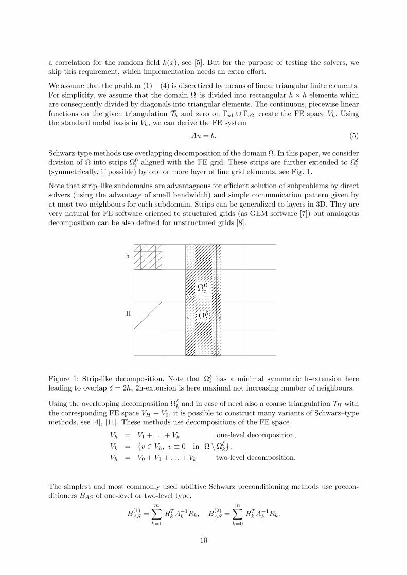
Schwarz-type methods use overlapping decomposition of the domain Ω. In this paper, we considerdivision of Ω into strips Ω0

i aligned with the FE grid. These strips are further extended to Ωδi

(symmetrically, if possible) by one or more layer of fine grid elements, see Fig. 1.

Note that strip–like subdomains are advantageous for efficient solution of subproblems by directsolvers (using the advantage of small bandwidth) and simple communication pattern given byat most two neighbours for each subdomain. Strips can be generalized to layers in 3D. They arevery natural for FE software oriented to structured grids (as GEM software [7]) but analogousdecomposition can be also defined for unstructured grids [8].

H

h

Figure 1: Strip-like decomposition. Note that Ωδi has a minimal symmetric h-extension here

leading to overlap δ = 2h, 2h-extension is here maximal not increasing number of neighbours.

Using the overlapping decomposition Ωδk and in case of need also a coarse triangulation TH with

the corresponding FE space VH ≡ V0, it is possible to construct many variants of Schwarz–typemethods, see [4], [11]. These methods use decompositions of the FE space

Vh = V1 + . . .+ Vk one-level decomposition,

Vk = v ∈ Vh, v ≡ 0 in Ω \ Ωδk ,

Vh = V0 + V1 + . . .+ Vk two-level decomposition.

The simplest and most commonly used additive Schwarz preconditioning methods use precon-ditioners BAS of one-level or two-level type,

B(1)AS =

m∑k=1

RTkA

−1k Rk, B

(2)AS =

m∑k=0

RTkA

−1k Rk.

10

For k = 1, . . . ,m, Rk is the restriction which selects degrees of freedoms lyingin Ωδ

k \ (Γu ∪ Γ0k), where Γ0

k = ∂Ωδk ∩ Ω is the inner boundary of Ωδ

k, Ak is the FE matrixcorresponding to subproblem on Ωδ

k with homogeneous Dirichlet boundary conditions on Γ0k.

For two-level preconditioner, RT0 represents the prolongation induced by imbedding VH ⊂ Vh

and A0 is the FE matrix for VH .

3 Analysis of the Schwarz methods

The analysis of the Schwarz methods for SPD problems usually uses the Lion’s lemma ([4],[11])and investigation of two properties

(P1) ∃K0 > 0 ∀v ∈ Vh ∃vk ∈ Vk , v = v1 + . . .+ vm :∑

∥ vk ∥2a≤ K0 ∥ v ∥2a

(P2) ∃K1 > 0 ∀v ∈ Vh ∀vk ∈ Vk , v = v1 + . . .+ vm : ∥ v ∥2a≤ K1

∑∥ vk ∥2a

where ∥ v ∥2a=√a(v, v), a is the SPD bilinear form from the variational formulation of the

problem (1) – (4). The constants can be used for estimation of the convergence or the conditionnumber of preconditioned systems, e.g.

cond(BASA) ≤ K0K1.

The estimation of K1 is easy. For our strip decomposition, we can take K1 = 3 for one-level de-composition and K1 = 4 for two-level decomposition. The investigation of stability constant K0

usually use a decomposition of unity

1 =

m∑k=1

θk, supp(θk) ⊂ Ωδk, ∥ θk ∥∞≤ 1, ∥ ∇θk ∥∞= O(δ−1)

and construct the decomposition of v ∈ Vh, v =∑vk, vk ∈ Vk with

vk = Πh(θkv) for one-level decomposition,

v0 = Qv, vk = Πh(θk(v − v0)) for two-level decomposition,

where Πh is linear interpolation C(Ω) → Vh, Q : Vh → V0 is e.g. a− or L2 projection. Thestandard analysis then uses elementwise investigation and Friedrichs-type estimate.

For our model problem and strip-like decomposition, it is easy to construct θk such that θk ≡ 1in Ωδ

k \∪

i=k Ωi, θk ≡ 0 outside Ωδk and θk linearly varying across the overlaping part of Ωδ

k.

4 Conclusions

In this paper, we consider a model problem and strip-like domain decomposition which allowsto clarify the influence of heterogeneity on efficiency of Schwarz type methods. For one-levelSchwarz, the analysis with the above mentioned partition of unity suggests that heterogeneityoutside overlapping regions Ωδ

k ∩ Ωδi does not influence efficiency of Schwarz methods (with

exact subdomain solvers). On the other hand, if the heterogeneity in the overlapping regionscan not be avoided, then the overlap as big as possible (preserving condition of at most twoneighbours subdomains) could be advantageous. These properties are now verified by numericalexperiments. For two level methods, there is more possibilities for adaptation to heterogeneity

11

and getting robust solvers, see e.g. [10], [1], [3]. Note that the defined strip decomposition is alsorobust with respect to orthotropy if strips are orthogonal to the ”weaker”direction [9].

Acknowledgement: This work is supported by the grants GACR105/09/1830 of the GrantAgency CR and the research plan AV0Z30860518 of the Academy of Sciences of the CzechRepublic.

References

[1] O. Axelsson, R. Blaheta, M. Neytcheva: Preconditioning of boundary value problems usingelementwise Schur complements. SIAM J. Matrix Analysis & Appl. 31, 767–789, 2009.

[2] O. Axelsson, R. Blaheta: Preconditioning of matrices partitioned in 2x2 block form: Eigen-value estimates and Schwarz DD for mixed FEM. Submitted.

[3] O. Axelsson, R. Blaheta, V. Sokol: Schwarz iterative methods for problems with heteroge-neous structure. In progress.

[4] R. Blaheta: Space decomposition preconditioners and parallel solvers. In: Numerical Methodsand Advanced Applications, M. Feistauer et al. (eds), Springer-Verlag, Berlin, 20–38, 2004.

[5] R. Blaheta, P. Byczanski, P. Harasim: Multiscale modelling of geomaterials and iterativesolvers. Proceedings of SNA’09, Institute of Geonics AS CR, Ostrava 2009.

[6] R. Blaheta, O. Jakl, J. Stary, K. Krecmer: Schwarz DD method for analysis of geocom-posites. In: Proceedings of the Twelfth International Conference on Civil, Structural andEnvironmental Engineering Computing B.H.V. Topping, L.F. Costa Neves and R.C. Barros,(eds.). Civil-Comp Press, Stirlingshire, UK, 2009.

[7] R. Blaheta, O. Jakl, R. Kohut, J. Stary: GEM – a Platform for Advanced MathematicalGeosimulations. In: Proceedings of the conference Parallel Processing and Applied Mathe-matics, PPAM 2009, to appear.

[8] G.A.A. Kahou, L. Grigori, M. Sosokina: A partitioning algorithm for block-diagonal matriceswith overlap. Parallel Computing 34, 332–344, 2008.

[9] T.P.A. Mathew: Domain decomposition methods for the numerical solution of partial di-fferential equations. Lecture Notes in Computational Science and Engineering, Springer,Berlin 2008.

[10] R. Scheichl, E. Vainikko: Additive Schwarz and aggregation-based coarsening for ellipticproblems with highly variable coefficients. Computing 80, 319–343, 2007.

[11] A. Toselli, O. Widlund: Domain Decomposition Methods - Algorithms and Theory. Springer-Verlag, Berlin 2005.

12

Flow over a rough surface

P. Bauer

Czech Technical University, Prague

Institute of Thermomechanics, AS CR, Prague

Abstrakt

We attempt to model a 2D rough surface by computing non-stationary Navier-Stokesflow over a periodic pattern. The solution is obtained by means of finite element method(FEM). We use non-conforming Crouzeix Raviart elements for velocity and piecewise con-stant elements for pressure. The resulting linear system is solved by multigrid method. Wepresent computational studies of the problem.

1 Introduction

We consider a polygonal domain Ω ⊂ R2 composed of multiple canyons as an approximationof a rough surface, and solve the incompressible Navier-Stokes equations for velocity u andpressure p on [0, T ]× Ω:

∂u(t, x)

∂t+ u(t, x) · ∇u(t, x)− νu(t, x) +∇p(t, x) = 0

∇ · u(t, x) = 0

u(0, x) = u0(x) x ∈ Ω

We set no-slip boundary condition for velocity on the terrain, Poiseuille profile on the inlet,Neumann condition on the outlet, and slip condition on the upper boundary.

2 Weak formulation of Navier-Stokes equations

Let X = (H(1)(Ω))2, V (uin) = u ∈ X : u |terrain= 0,u |inlet= uin,u |upper ·n = 0, Q = L2(Ω).We set the following forms:

(∇u,∇v) =∫Ω

2∑i,j=1

∂ui∂xj

∂vi∂xj

, b(u,v,w) = 12

∫Ω

2∑i,j=1

(uj∂vi∂xj

wi − ujvi∂wi∂xj

).

We use the backward Euler difference for the time derivative ∂u(tn,x)∂t ≈ un−un−1

τ where tn = nτ .For each timestep tn, we seek un ∈ V (uin) and p

n ∈ Q, such that ∀v ∈ V (0), ∀q ∈ Q:

(un,v) + τb(un−1,un,v) + τ(∇un,∇v)− τ(pn,∇ · v) = (un−1,v)

(q,∇ · un) = 0

Let index h denote the respective finite-dimensional spaces V h(uin), Qh, and the corresponding

functions unh, p

nh. We use the upwinding technique proposed by [2], based on dual elements Rl

given by the barycentric nodes of the original mesh (Fig. 1).

13

We introduce wh ∈ V h(uin) to respresent inhomogeneous Dirichlet data. Taking vh = uh−wh ∈V h(0), the discrete problem for each timestep tn rewritten in the matrix form stands:

Mvnh + τN(un−1

h )vnh + τAvn

h + τBTpnh = f , (1)

Bvnh = g,

where

f = M(vn−1h +wn−1

h −wnh)− τN(un−1

h )wnh − τAwn

h ,

g = −Bwnh .

3 Numerical solution using FEM

We choose non-conforming Crouzeix-Raviart elements (Fig. 1) to approximate the componentsof velocity and piecewise constant elements for pressure.

Figure 1: a) Lumped regions, b) Crouzeix-Raviart element.

We use multigrid solver based on Vanka-type smoother to solve the linear system (1). An ex-tension for higher order elements can be found in [3].

4 Numerical results

We consider a periodic pattern composed by seven square canyons. We show the developmentof the flow over the pattern for Re = 104.

5 Conclusion

We investigate the flow over periodic structures as the means for parametrization of roughsurfaces in models of larger scale in cooperation with the Institute of Thermomechanics of theAcademy of Sciences of the Czech Republic.

Acknowledgement: This work has been supported by the research direction project AppliedMathematics in Technical and Physical Sciences of the Ministry of Education of the CzechRepublic No. MSM6840770010.

14

Figure 2: |u(t)| at time t = 24, 32, 40.

15

References

[1] F. Brezzi, M. Fortin, Mixed and hybrid finite-element methods, Springer Verlag, New York(1991)

[2] F. Schieweck, L. Tobiska, An optimal order error estimate for upwind discretization of theNavier-Stokes equation, Numerical methods in partial differential equations y.12 n.4 (1996),407–421

[3] V. John, P. Knobloch, G. Matthies, and L. Tobiska, Non-Nested Multi-Level Solvers forFinite Element Discretisations of Mixed Problems, Computing 68 (2002), 313–341

16

On iterative QR pre–processing in the

parallel block–Jacobi SVD algorithm

M. Becka, G. Oksa, M. Vajtersic

Institute of Mathematics, Slovak Academy of Sciences, Bratislava

1 Introduction

Recently, an efficient version of the parallel two-sided block Jacobi SVD algorithm with pre-processing was proposed in [4]. When computing all singular values together with all right andleft singular vectors of a rectangular matrix A, the pre-processing step consists of the parallelcomputation of the QR factorization (QRF) with column pivoting (CP) followed A by theoptional LQ factorization (LQF) of R-factor (this is called the QRLQ step). The parallel A two-sided block Jacobi method with dynamic ordering (cf. [1]) is then applied to the R-factor (orL-factor). The purpose of pre-processing is to concentrate the Frobenius norm near the matrixdiagonal so that the Jacobi algorithm may need substantially less parallel steps for convergencethan in the case without pre-processing.

However, to perform optimally, A the parallel A QRF (or LQF) and the parallel two-sided blockJacobi method need different data layouts. Having p processors, A the Jacobi algorithm performsvery well when the matrix is distributed using the one-dimensional block column distribution. Inthis case, most of the computations can be performed locally. But this data distribution is notwell suited for the serialized block column-oriented parallel QRF. Instead, a block cyclic matrixdistribution on a process grid r × c A with p = rc, r, c ≥ 1, is needed so that all processorsremain busy during the whole parallel QR (or LQ) factorization.

Optimal parameters for the pre-processing step need to be found experimentally for a givenparallel architecture. For a cluster of modern computational nodes, it is shown that their valuesare about nb = 100 and r ≤ c, r = max, i.e., r is maximized so that both r and c are as closeto

√p as possible. Numerical experiments suggest that the efficiency of a pre-processing step

depends on the distribution of singular values (SVs). In contrast, the dependence on the conditionnumber κ is only mild. The optimal parameters were then used in the pre-processed parallel two-sided block-Jacobi SVD algorithm; its performance was tested for six various distributions ofSVs and for well-conditioned (κ = 101) as well as ill-conditioned (κ = 108) random, square,real matrices of order n = 4000 and 8000 using p = 8 and 16 processors, respectively, withthe constant ratio n/p = 500. The largest savings in the number of parallel iteration stepsneeded for the convergence of the whole algorithm were obtained for matrices with a multiplemaximal/minimal SV regardless to κ. In these two cases, our algorithm performs better orequally well as the ScaLAPACK routine PDGESVD. However, it is shown experimentally thatfor other four distributions of SVs, the parallel two-sided block-Jacobi SVD algorithm with theoptimal pre-processing and dynamic ordering is about 1.2–2.3 times slower than the ScaLAPACKroutine.

The un-pivoted QRLQ pre-processing step can be re-formulated and extended to the QR ite-ration (QRI). Using a limited number of QRI steps in the pre-processing can lead to even largerreduction of the off-diagonal Frobenius norm and to the faster convergence of the subsequentJacobi algorithm with dynamic ordering for certain distributions of SVs. In the serial case, the

17

use of the QRI for the estimates of SVs and singular vectors has been analyzed, e.g., in [2, 3]. Toour knowledge, up to now nobody extended its use as the pre-processing method for computingthe SVD in parallel. We have implemented the QRI in front of the parallel two-sided block-Jacobi algorithm with dynamic ordering, and we report results for a set of matrices mentionedabove. In general, the use of about 6 QRI steps can be recommended before switching to theJacobi algorithm. Such a strategy can significantly decrease the total parallel execution time ofthe whole algorithm.

2 Parallel algorithm with dynamic ordering

When using p processors and the blocking factor ℓ = 2p, a given matrix A is cut column-wiseand row-wise into an ℓ× ℓ block structure. Each processor contains exactly two block columnsof dimensions m× n/ℓ so that ℓ/2 SVD subproblems of block size 2× 2 are solved in parallel ineach iteration step.

At the beginning of each parallel iteration step, it is necessary to map one 2 × 2 block SVDsubproblem to each of p processors. This can be achieved by some type of ordering. The so-calleddynamic ordering is based on the maximum-weight perfect matching that operates on the ℓ× ℓupdated weight matrixW using the elements ofW+W T , where (W+W T )ij = ∥Aij∥2F+∥Aji∥2F.As shown in [1], this approach leads to a maximum decrease of the off-diagonal Frobenius normin each parallel iteration step. Moreover, the optimal algorithm for finding the ordering hascomplexity O(ℓ3).

The convergence of the whole process can be enhanced by a suitable pre-processing of matrix A.As discussed in [4], the QR factorization with column pivoting (QRFCP) can be applied to Aat the beginning of computation. Then, the SVD of the matrix R is computed by the PTBJAwith dynamic ordering. In the final step, some post-processing in the form of matrix-matrixmultiplication is required to obtain the SVD of A.

Alternatively, after the QRFCP of A, one can apply the LQF of R-factor (without columnpivoting). Next, the SVD of L is computed by our parallel PTBJA with dynamic ordering. Toobtain the SVD of A, two matrix-matrix multiplications are needed in the final post-processingstep.

The purpose of the pre-processing step is twofold. First, for rectangular matrices of order m×n,m ≥ n, the R-factor (L-factor) is a square matrix of order n, which means that for m≫ n hugesavings in storage requirements, matrix multiplications and computation of 2 × 2 block SVDscan be achieved. Second, after the QRFCP (followed by the optional QLF of the R-factor), theFrobenius matrix norm is usually well concentrated near the matrix diagonal, so that only fewiteration steps in the parallel two-sided block-Jacobi algorithm are needed for convergence.

3 Optimal data layout for pre-processing

When using p processors with the matrix block cyclic distribution of type 1× p (i.e., the wholeblock columns are stored in processors), it is immediately clear that the computation of theblock QRF is serialized and synchronized. When the blocking factor in the iterative part of theJacobi algorithm is ℓ = 2p (i.e., each processor stores two block columns), and the block sizefor the QRF is nb, then processor i, 0 ≤ i ≤ p − 1, starts the QRF of its submatrix at step2⌈n/ℓ⌉i and finishes it at step 2⌈n/ℓ⌉(i+ 1) (one step here means the processing of one matrix

18

column). During this computation, processor i sends 2⌈n/ℓ⌉/nb-times data to processors to itsright for computing updates. At any given time, only one processor computes the QRF; all otherprocessors are computing only the updates and they have to wait for data. As the computationis column-oriented and proceeds from left to right, more and more processors become idle duringthe computation of the block QRF. This is a highly inefficient use of the computational power.

To increase the efficiency in the pre-processing step, one should use a matrix cyclic block dis-tribution with block size nb on a process grid r × c, r, c ≥ 1, with p = rc, where r and c is thenumber of processors in a process row and column, respectively. This type of data distributionis required by all ScaLAPACK matrix routines. Such a data distribution eliminates the synchro-nization in computing the block QRF and can lead to a better use of computational resourcesand thus to a faster computation. On the other side, the broadcast of updating data becomesmore complex because it needs to be done both across process rows and columns. Moreover, inthe triangularization of a given block column A1 of width nb, all processors in the appropriateprocess column are involved and they have to communicate. Despite these differences as com-pared with the process grid 1× p, the parallel block QRF (with or without column pivoting) ona process grid r × c, r, c ≥ 1, p = rc, can take substantially less time.

We will report our results for all possible combinations of r and c for a given number of processorsp together with a variable block column width nb. Regardless to the number of processors anddistribution of singular values, the minimum total parallel execution time was achieved fornb = 100 and the process grid r × c with r ≤ c, r closest to

√p.

4 Numerical experiments with the optimal data layout

We have implemented the parallel two-sided block-Jacobi SVD algorithm (PTBJA) with pre-processing on the Woodcrest Cluster at Regionales Rechenzentrum Erlangen (RRZE), Erlangen-Nuernberg University, Germany. The Woodcrest Cluster consists of 217 computational nodes,each with two Xenon 5160 Woodcrest chips (4 cores organized in 2 dual cores) running at3.0 GHz. Each dual core contains 4 MB shared Level 2 cache, 8 GB of RAM and 160 GB oflocal scratch disk. The Infiniband interconnection network has the bandwidth of 10 GBit/s perlink and direction.

Each test matrix was generated by the ScaLAPACK routine DLATMS as a matrix product usinga given distribution of SVs chosen from a group of six possible types, and two random orthogonalmatrices with elements from the normal distribution N(0, 1). Two condition numbers were used:κ = 101 and κ = 108.

We will report and comment detailed results from our numerical experiments. These experimentscan be divided in two groups. In the first group, four variants of the PTBJA with dynamicordering were tested: without any pre-processing, with the pre-processing consisting of the QRFwith CP, and with the pre-processing where the QRF with/without CP was followed by the LQFof R-factor. For matrices with a multiple maximal/minimal SV, the use of optimal parametersin the pre-processing step (the QRF without CP following by the LQF of R-factor) enabled toachieve the performance better or comparable to that of the ScaLAPACK routine PDGESVD. Forother distributions of SVs, even the QRFCP + the LQF of R-factor did not lead to a significantdecrease of a number of iterations so that the pre-processed PTBJA with dynamic ordering wasabout 1.2–2.3 times slower than the ScaLAPACK routine PDGESVD.

In the second group of experiments, the un-pivoted QRLQ pre-processing was re-formulated andextended to the QR iteration (QRI). There is a well-known connection between the QRI and

19

the QR algorithm applied to a specific sequence of symmetric, positive definite matrices, whichenables to use the convergence theory of the QR algorithm for the explanation of experimentalresults. Specifically, the convergence of the QRI is largely enhanced in the case of multiple SVs(or cluster of close SVs) and in presence of large gap(s) between any consecutive SVs, whichis rather typical for ill-conditioned matrices. In such situation it can happen that the SVD iscomputed only by using, say, 4 QRI steps, without invoking the Jacobi algorithm at all. Ingeneral, the use of about 6 QRI steps can be recommended in the pre-processing, followed bya (quite limited) number of parallel iterations in the Jacobi algorithm with dynamic ordering.Such a strategy usually leads to a significant reduction of the total parallel execution time ofthe whole algorithm for almost all six tested distributions of SVs.

Acknowledgments: Our special thanks go to Prof. Dr. Ulrich Ruede from Erlangen-NuernbergUniversity for his kind permission and help in using the Woodcrest Cluster. First two authorswere supported by the grant no. APVV− 0532− 07 from the Agency for Science and Research,Slovakia.

References

[1] M. Becka, G. Oksa, M. Vajtersic: Dynamic ordering for a parallel block-Jacobi SVD algo-rithm. Parallel Computing, 28 243–262, (2002).

[2] S. Chandrasekaran, I.C.F. Ipsen: Analysis of a QR algorithm for computing singular values.SIAM J. Matrix Anal. Appl., 16(2), 20–535, (1995).

[3] D. A. Huckaby, T. F. Chan: On the convergence of Stewart’s QLP algorithm for approxi-mating the SVD. Num. Alg., 32, 287–316, (2003).

[4] G. Oksa, M. Vajtersic: Efficient pre-processing in the parallel block-Jacobi SVD algorithm.Parallel Computing, 32, 166–176, (2006).

20

Moving boundaries in material science

M. Benes

Department of Mathematics, Faculty of Nuclear Sciences and Physical Engineering,Czech Technical University in Prague, Trojanova 13, 120 00 Praha 2, Czech Republic

benesmic@kmlinux.fjfi.cvut.cz

The presentation discusses mathematical modelling and numerical simulation of two classes offree-boundary problems arising in material science, which are related to the microstructure for-mation in solidification of crystalline materials, and to the dislocation dynamics in the crystallinelattice.

The discussed problems occurring in the context of material science have a similar evolutionlaw. This law generally written in the form

vΓ = −κΓ + F,

is known to describe the motion of curves or surfaces by mean curvature (here denoted by κΓ,whereas vΓ denotes the normal velocity and F a forcing term). The law together with its variantsincluding anisotropy is being extensively studied from the mathematical as well as applicationviewpoint. We present formulation of mathematical models as well as their numerical solutiondemonstrating agreement with the experimental understanding of the studied phenomena.

21

Tvarova optimalizace pro 3D kontaktnı problem

diskretizovany metodou hranicnıch prvku

P. Beremlijski, M. Sadowska

Katedra aplikovane matematiky, VSB - Technicka univerzita Ostrava

1 Uvod

V prıspevku se zabyvame ulohou diskretnı tvarove optimalizace trojrozmerneho pruzneho telesav jednostrannem kontaktu s tuhou prekazkou. Pro diskretizaci kontaktnı ulohy jsme pouzilimetodu hranicnıch prvku. Aplikace metody hranicnıch prvku na kontaktnı ulohy muzeme najıtnaprıklad v [2, 5]. Pro maly koeficient trenı ma diskretizovana kontaktnı uloha s Coulombovymtrenım jedine resenı, ktere je navıc zavisle lokalne lipschitovsky na rıdıcı promenne popisujıcıtvar pruzneho telesa. Dıky jedinemu resenı diskretnı ulohy pro fixovanou rıdıcı promennou,muzeme pouzıt tzv. prıstup implicitnıho programovanı, ktery je zalozen na minimalizaci ne-hladke funkce slozene z cenove funkce a jednoznacneho zobrazenı, ktere rıdıcı promenne prirazujeresenı diskretnı ulohy, tzn. stavove promenne. Pro minimalizaci nehladke funkce jsme pouzilibundle trust metodu. K zıskanı subgradientnı informace, kterou metoda vyzaduje, je nutnopouzıt Morduchovicova a Clarkeova kalkulu.

2 Kontaktnı uloha s Coulombovym trenım

Bud’ O zvolena trıda omezenych oblastı Ω ⊂ R3 s lipschitzovskou hranicı Γ slozenou ze trınavzajem disjunktnıch castı Γd, Γn a Γc (viz obr. 1). Oblast Ω ∈ O je vyplnena homogennımizotropnım materialem a ma tvar

”kvadru“ se spodnı volnou castı Γc = Γc(Ω), jejız tvar bude na-

vrhovan pomocı zvolenych prıpustnych funkcı α : R 7→ R, kde R oznacuje pravouhly prumet Ωdo roviny xy. Cast hranice Γd ∪ Γn je pevna.

Obrazek 1: Geometrie oblasti Ω ∈ O.

Na Γd budeme uvazovat homogennı Dirichletovu podmınku ve vsech souradnych smerech, na Γn

pusobı povrchove sıly h ∈ [L2(Γn)]3 a podel Γc je teleso

”podepreno“ tuhou prekazkou R2 ×R−

(viz obr. 1), pricemz mezi telesem a prekazkou uvazujeme Coulombovo trenı dane koeficientem F .Funkce u(Ω) tedy vyhovuje systemu homogennıch rovnic rovnovahy Lu = 0 linearnı homogennıizotropnı elastostatiky, predepsane Dirichletove resp. Neumannove podmınce na Γd resp. Γn,unilateralnım kontaktnım podmınkam

u3(x) ≥ −x3, T3(x) ≥ 0, T3(x)(u3(x) + x3) = 0 pro kazde x = (x1, x2, x3) ∈ Γc(Ω),

22

a Coulombovu zakonu trenıpokud ut(x) := (u1(x), u2(x), 0) = 0, pak ∥Tt(x) := (T1(x), T2(x), 0)∥ ≤ FT3(x)

pokud ut(x) = 0, pak Tt(x) = −FT3(x)ut(x)/∥ut(x)∥

pro kazde x ∈ Γc(Ω). Vektor T(x) = (T1(x), T2(x), T3(x)) znacı povrchove napetı v x ∈ Γc(Ω).

3 Slaba hranicnı formulace stavoveho problemu

Slabe resenı u ∈ [H1(Ω)]3 systemu homogennıch rovnic rovnovahy linearnı homogennı izotropnıelastostatiky splnuje Greenuv reprezentacnı vztah

ul(x) =

∫Γ

(γ1u(y), Ul(x, y)) dsy −∫Γ

(γ0u(y), γ1,yUl(x, y)) dsy, x ∈ Ω, l = 1, 2, 3, (1)

kde U je fundamentalnı resenı linearnı elastostatiky zname jako Kelvinuv tensor:

Ukl(x, y) :=1 + ν

8πE(1− ν)

((3− 4ν)

δkl∥x− y∥

+(xk − yk)(xl − yl)

∥x− y∥3

), k, l = 1, 2, 3,

γ0 : [H1(Ω)]3 7→ [H1/2(Γ)]3 je operator stopy a

γ1 : v ∈ [H1(Ω)]3 : Lv ∈ [L2(Ω)]3 7→ [H−1/2(Γ)]3

je operator prıslusneho povrchoveho napetı splnujıcı pro v ∈ [C∞(Ω)]3

(γ1v)i (x) =3∑

j=1

σij(v, x)nj(x), x ∈ Γ, i = 1, 2, 3;

nj(x) je slozka vnejsıho jednotkoveho normaloveho vektoru a σij je slozka tensoru napetı.

Aplikacı operatoru γ0 a γ1 na (1) zıskame (dle [6]) hranicnı vztah

γ1u = S(γ0u) na Γ,

kde S : [H1/2(Γ)]3 7→ [H−1/2(Γ)]3 je Steklovuv-Poincareho operator, ktery lze reprezentovatjako

S = D + (1

2I +K ′)V −1(

1

2I +K);

V je operator jednoduche vrstvy, K je operator dvojvrstvy, K ′ je operator adjungovany ke Ka D je tzv. hypersingularnı operator. Definice a vlastnosti techto operatoru jsou k nalezenı v [6].

Definujme nynı W (Ω) := [H1/20 (Γ(Ω),Γd)]

3 a X(Ω) := φ ∈ L2(R) : existuje v ∈W (Ω) takove,ze na Γc(Ω) platı φ = v3. Bud’ dale X ′

+(Ω) kuzel kladnych funkcionalu z dualu X ′(Ω). Slabymhranicnım resenım kontaktnıho stavoveho problemu z 2. kapitoly rozumıme libovolnou dvojici(u, λ) ∈W (Ω)×X ′

+(Ω) vyhovujıcı systemu∫

Γ(Ω)

(Su, v− u) ds+ ⟨Fλ, ∥vt∥ − ∥ut∥⟩ ≥∫Γn

(h, v− u) ds+ ⟨λ, v3 − u3⟩ ∀v ∈W (Ω)

⟨µ− λ, u3 + α⟩ ≥ 0 ∀µ ∈ X ′+(Ω),

kde ⟨·, ·⟩ je dualitnı parovanı mezi prostory X(Ω) a X ′(Ω), v3(x′) := v3(x

′, α(x′)) a vt(x′) :=

(v1(x′, α(x′)), v2(x

′, α(x′)), 0), x′ ∈ R.

23

4 Diskretnı tvarova optimalizace pro kontaktnı ulohu s Coulom-bovym trenım

Nez si zformulujeme nasi ulohu tvarove optimalizace, zapisme nas stavovy problem formou zo-becnene rovnosti. K tomu diskretizujeme stavovou ulohu a pote zavedeme rozdelenı vektoruposunutı u na (ut,uν), kde ut prıslusı tecnemu posunutı a uν odpovıda normalovemu posunutı.Nasledne vyeliminujeme volne uzly, tj. budeme se zabyvat pouze kontaktnımi uzly (jejich pocetje p). Diskretizovanou stavovou ulohu muzeme popsat zobrazenım S : α ∈ Rd → (ut,uν ,λ) ∈R4p (tvaru oblasti Ω, ktery je urcen rıdıcım vektorem α ∈ Uad, je prirazeno resenı kontaktnıulohy s Coulombovym trenım (ut,uν ,λ) (stavove promenne)). Zobrazenı S je pro male koefici-enty trenı lokalne lipschitzovske. Diskretizovanou stavovou ulohu muzeme ekvivalentne popsatzobecnenou rovnostı:

0 ∈ Att(α)ut +Atν(α)uν − Lt(α) + Q(ut,λ)0 = Aνt(α)ut +Aνν(α)uν − Lν(α)− λ0 ∈ uν +α+NRp

+(λ),

(2)

kde A(α) ∈ R3p×3p a L(α) ∈ R3p jsou matice tuhosti a vektoru prave strany, ktere jsme zıskalipo diskretizaci stavove ulohy metodou hranicnıch prvku,

Q(ut1,ut2,λν) = ∂(ut1,ut2)j(ut1,ut2,λν), j(ut1,ut2,λν) = Fp∑

i=1

λi||(uit1,u

it2)||

a NRp+je standardnı normalovy kuzel.

Nynı si popisme ulohu tvarove optimalizace. Hledame navrhovou promennou α rıdıcı tvarBezierovy plochy, kterou je urcena kontaktnı hranice Γc, tzn. i tvar telesa Ω, pro kterou nabyvacenovy funkcional J (α,S(α)) sveho minima. Ulohu diskretnı tvarove optimalizace pro kontaktnıulohu s Coulombovym trenım pak popıseme takto:

minΘ(α)

s omezenımα ∈ Uad,

kde Θ(α) := J (α,S(α)). Necht’ funkcional J je spojite diferencovatelny. K resenı teto ne-hladke ulohy byla pouzita bundle trust metoda. Tato iteracnı metoda potrebuje rutinu, kterav kazdem kroce vypocte hodnotu cenoveho funkcionalu (k tomu potrebujeme vyresit diskre-tizovanou stavovou ulohu) a jeden (libovolny) Clarkeuv subgradient z Clarkeova zobecnenehogradientu ∂Θ(α). Pro jeho konstrukci pouzijeme tvrzenı

∂Θ(α) = ∇1J (α,S(α)) + C T∇2J (α,S(α))|C ∈ ∂S(α)

(viz [3]). Dale vyuzijeme nehladkeho kalkulu B. Morduchovice (viz [4]).

Protoze platı ∅ = D∗S(α)(y∗) pro vsechna y∗ a conv (D∗S(α)) (y∗) = C Ty∗|C ∈ ∂S(α),stacı nalezt jeden prvek z mnoziny D∗S(α)(∇2J (α,S(α))). Hledanı prvku limitnı koderivace

D∗S(α)(y∗) := x ∗ ∈ Rd | (x ∗,−y∗) ∈ NGr S(α),

kde Gr S je graf S a NGr S je limitnı normalovy kuzel, je znacne komplikovane a vyuzıva se prinem zapisu zobrazenı S pomocı zobecnene rovnosti (2) (podrobne viz [1]).

24

5 Zaver

Ve 3D uloze tvarove optimalizace nenı mozne pro citlivostnı analyzu vyuzıt po castech spojitoudiferencovatelnost zobrazenı S, ktere rıdıcımu vektoru prirazuje stavove promenne, jako ve 2Dverzi teto ulohy. Proto jsme pro citlivostnı analyzu optimalizacnı ulohy, kterou se zabyvamev teto praci, museli pouzıt Morduchovicova kalkulu. Pro citlivostnı analyzu je nutne vypocıstparcialnı derivace matice tuhosti a vektoru prave strany, ktere zıskame pri diskretizaci stavoveulohy metodou hranicnıch prvku, podle jednotlivych rıdıcıch promennych. V teto praci jsme tytoderivace zıskali numericky. V budoucnu bychom chteli odvodit vztahy pro analyticky vypocettechto derivacı.

Podekovanı: Tato prace byla podporena GA CR 201/07/0294 a MSMT MSM6198910027.

Reference

[1] P. Beremlijski, J. Haslinger, M. Kocvara, R. Kucera, J. Outrata: Shape Optimization inThree-Dimensional Contact Problems with Coulomb Friction. SIAM Journal on Optimi-zation 20(1), 416–444, 2009.

[2] J. Bouchala, Z. Dostal, M. Sadowska: Scalable Total BETI Based Algorithm for 3D CoerciveContact Problems of Linear Elastostatics. Computing 85, 189–217, 2009.

[3] F.H. Clarke: Optimization and Nonsmooth Analysis. J. Wiley & Sons, 1983.

[4] B.S. Mordukhovich: Variational Analysis and Generalized Differentiation, Volumes I and II.Springer-Verlag, 2006.

[5] C. Eck, O. Steinbach, W.L. Wendland: A Symmetric Boundary Element Method for ContactProblems with Friction. Math Comput Sim 50, 43–61, 1999.

[6] O. Steinbach: Numerical Approximation Methods for Elliptic Boundary Value Problems,Finite and Boundary Elements. Springer-New York, 2008.

25

A parametric study of the dimensionless

closed gas-liquid system

M. Biak, D. Janovska

Department of Mathematics, Institute of Chemical Technology, Prague

1 Introduction

In the original model introduced in [1], the solution depends on ten parameters. The dimension-less formulation significantly reduces the number of parameters only to four. Another obviousadvantage is the formulation independency on the model scale.

We study the dependence of the solution of the dimensionless formulation on a given parameterset. All simulations are performed in Matlab software package, namely we use a modified versionof the program developed by Petri T. Piiroinen and Yuri A. Kuznetsov, see [3].

2 Transformation of the model equations into a dimensionlessform

Let us start with the original dimensional Filippov system that describes the closed gas-liquidsystem. For the detailed derivation of the model equations, see [1], [2].

F :d

d t

(MG

ML

)=

f (1)(MG,ML), φ(MG,ML) < 0,

f (2)(MG,ML), φ(MG,ML) > 0,(1)

where

f (1) =

FG − kGx

(MGRT

V −ML/ρL− Pout

)FL

, (2)

f (2) =

FG

FL − kLx

(MGRT

V −ML/ρL− Pout

) , (3)

φ(MG,ML) =ML − ρLVd. (4)

Let p = (FG, FL, ρL, V, Vd, T, Pout, x, kL, kG)T, p ∈ R10, be a row vector of the parameters. We

consider the Filippov system F dependent on p:

F(p) :d

d t

(MG

ML

)=

f (1)(MG,ML, p), φ(MG,ML, p) < 0,

f (2)(MG,ML, p), φ(MG,ML, p) > 0,(5)

where

f (1)(MG,ML, p) =

FG − kGx

(MGRT

V −ML/ρL− Pout

)FL

, (6)

26

f (2)(MG,ML, p) =

FG

FL − kLx

(MGRT

V −ML/ρL− Pout

) , (7)

φ(MG,ML, p) =ML − ρLVd. (8)

Now, we can define the dimensionless state variables MG, ML, t,

MG :=MG MG, ML :=M

L ML, t := t t. (9)

If we choose the scaling

FGt

MG

= 1, FLt

ML

= 1,ρLV

ML

= 1, (10)

we obtain a row vector of the dimensionless parameters p = (αG, αL, βL, βG, γ)T, p ∈ R5, where

αG = kGxtM

GRTρL(M

L)2

= kGxFGRTρL

F 2L

, (11)

αL = kLxtM

GRTρL(M

L)2

= kLxFGRTρL

F 2L

, (12)

βL = kLxPoutt

ML

=kLxPout

FL, (13)

βG = kGxPoutt

ML

=kGxPout

FL, (14)

γ =VdV. (15)

The dimensionless Filippov system F dependent on p ∈ R5 has the form:

F(p) :d

d t

(MG

ML

)=

f (1)(MG, ML, p), φ(MG, ML, p) < 0,

f (2)(MG, ML, p), φ(MG, ML, p) > 0,(16)

where

f (1)(MG, ML, p) =

1− αGMG

1− ML

+ βG

1

, (17)

f (2)(MG, ML, p) =

1

1− αLMG

1− ML

+ βL

, (18)

φ(MG, ML, p) = ML − γ. (19)

It is useful to separate the parameters FG and FL in (11) and (12) in such a way that they mayvary independently. Let us set

K :=kGkL

, (20)

M :=αL

β2L=FGRTρLkLxP 2

out

. (21)

27

We can express αL and βG from these two equations,

αL =Mβ2L , (22)

βG = KβL. (23)

We obtain four dimensionless parametrs, i. e. the row vector q = (M,K, βL, γ)T, q ∈ R4. The

resulting dimensionless Filippov system F then depends only on q. It has the form

F(q) :d

d t

(MG

ML

)=

f (1)(MG, ML, q), φ(MG, ML, q) < 0,

f (2)(MG, ML, q), φ(MG, ML, q) > 0,(24)

where

f (1)(MG, ML, q) =

1−KMβ2LMG

1− ML

+KβL

1

, (25)

f (2)(MG, ML, q) =

1

1−Mβ2LMG

1− ML

+ βL

, (26)

φ(MG, ML, q) = ML − γ. (27)

3 Conclusions

We manage to reduce the number of parameters from ten to only four. The system F(q) exhibitsa certain slow-fast character. In simulations, it turned out, that two of these parameters, namelyM and βL, substantially affect the behaviour of the system.

Acknowledgement: The work is a part of the research project MSM 6046137306 financed byMSMT, Ministry of Education, Youth and Sports, Czech Republic.

References

[1] K.M. Moudgalya, V. Ryali: A class of discontinuous dynamical systems I. An ideal gas-liquidsystem. Chemical Engineering Science 56, 3595–3609, 2001.

[2] M. Biak, D. Janovska: Filippov dynamical systems. In: R. Blaheta, J. Stary (ed.): Seminaron Numerical Analysis & Winter School/Proceedings of the Conference SNA’09, Ostrava,February 2-6, 2009 Appendix, 1–4.

[3] P.T. Piiroinen, Yu.A. Kuznetsov: An event-driven method to simulate Filippov systems withaccurate computing of sliding motions, ACM Trans. Math. Software 34(13), 1–24, 2008.

28

Parameter identification in heat flow with a geo-application

R. Blaheta, R. Kohut

Institute of Geonics AS CR, v.v.i., Ostrava, Czech Republic

1 Introduction

Problems of identification of material parameters (mostly parameters appearing in constitutiverelations) have application in many fields of engineering including investigation of processes ina rock mass. This paper outlines the structure of parameter identification problems, methodsfor their solution and describes an identification problem from geotechnics, which will serveas a realistic model example for the showing behaviour of a selected parameter identificationmethod.

Most generally, the identification problems appear in investigation of physical processes in mate-rial environment. The processes are described by the state variables u and driven by the controlvariables f . The material is characterized by parameters κ. Direct problems focus on compu-tation of u = uh(κ) = uh(κ, x, t), where (x, t) gives space and time localization, if f and κ areknown. On the opposite, identification problems use the knowledge of f and some partial aprioriknowledge on the state variable u for (partial or full) determination of κ.

If the apriori information about the state variable u is given by the vector d = (di) of measuredvalues di ∼ u(xi, ti), then the search for the unknown material parameters can be formulated asthe following minimization problem

f(κ) =∥ Muh(κ)− d ∥−→ minκ∈K

. (1)

Above, M is an observation operator, which select from uh values corresponding to d.

In contrary to direct problems, it is known that some identification problems are not well posed,which means that some of the following properties can be violated:

• there exists solution of the problem,

• the solution is unique,

• the solution is stable under small changes of input data.

Although the properties of the minimization problems can be difficult to analyse, a lot of differentiterative techniques can be used for the minimization (1) (mostly without theoretical proof ofconvergence). The range of applicable methods includes

• gradient methods, e.g. Gauss-Newton, Levenberg-Marquardt, conjugate gradients, see [3],[4], [6], [7],

• gradient-free direct method, e.g. Nelder-Mead simplex method [3],

• stochastic methods e.g. [5], genetic algorithms e.g. [6].

In this paper, we shall show the solution of the identification problem, described in the nextsection, by means of least-square formulation (1) and application of the Nelder-Mead algorithm.

29

2 A model identification problem

The in-situ Aspo Pillar Stability Experiment (APSE) has been performed at SKBs Aspo HardRock Laboratory in south eastern Sweden with the aid of investigation of granite mass damagedue to mechanical and thermal loading. The measured data are now used for validation ofmathematical models within the DECOVALEX 2011 international project. APSE used electricalheaters to increase temperatures and induce stresses in a rock pillar between holes (Fig. 1)until its partial failure. To determine accurately the temperature changes, a heat flow model isformulated and monitored temperatures are used for identification of heat flow parameters (heatcapacity, heat conduction coefficient, heat convection into the holes). The identification shouldprovide parameters taking into account water bearing fractures and water flow and calibrate themodel. More details and another approach to the model calibration can be found in [1].

dryside

wetside

Figure 1: The APSE model - detail of the FE grid around the pillar (GEM software [2]) andplan view on the pillar, holes, location of heaters and points of temperature measurement.

The exploited APSE model, realized by GEM software [2], considers domain of 105×125×118 mand 99 × 105 × 59 nodes. The grid is refined around the pillar, see Fig. 1. The heaters areproducing heat which varies in time. The model assumes original temperature 14.5C on theouter boundaries, zero flux onto the tunnel and nonzero flux given the convection onto the holes.The initial condition is given again by the temperature 14.5C.

Monitoring of the temperatures during two month heating phase of APSE is essential for calib-ration of the thermal model. There are 14 temperature monitoring positions and temperaturesare measured in 12 time moments. Altogether 168 values of temperature measurement (vector d)are used for parameter identification, which according to (1) can be written as follows

f = f(λ1, c1, λ2, c2, λ3, c3,H1,H2,H3) =

(∑i

[uh(xi, ti)− di]2

)0.5

−→ min . (2)

The material parameters represent different conductivity λ and heat capacity c for dry and wetside of model (according to Fig.1.). The rock in the right hole had yielded from a depth ofapproximately 0.5 m down to 3 m which motivates to introduce third type of material withdifferent λ and c for the damaged part of the pillar. We supposed heat conduction between rockand air in excavated holes determined by different values of the heat conduction coefficient H forindividual holes with third coefficient corresponding to surface for the above mentioned damagedpart of the pillar. It gives 9 material parameters of the cost functional f in (2).

30

3 The optimization method and numerical results

For finding the minimum (or at least realizing sufficient decrease) of the cost functional (1), (2) re-presenting agreement between the measured and computed values, we use Nelder-Mead simplexmethod, see e.g. [3]. To guarantee the positivity of the parameters, we use exponential transfor-mation, i.e. finding x such that p = ex is the required parameter. As the parameters have quitedifferent orders, we scale the capacity c for having all parameters in order of units.

The Nelder-Mead iterations are stopped when both decrease of the cost functional f is small(below εf ) and changes of parameters are small (below εp). To find very accurate approximationof the parameters, we stop iterations with εf = 0.001 and εp = 0.01. With a physical initialguess, it requires 764 iterations. The reached minimum value was f = 33.599. The obtainedmaterial parameters can be seen in Table 1, the convergence behaviour is illustrated in Fig. 2.

We also tested the sensitivity of the cost functional F to change of individual parameters in thevicinity of the computed optimum, i.e. we fixed 8 values from Table 1 and show dependenceof f on the remaining one. In Fig. 3, we can see that with respect to λ1 and c1, we get stableminimum (a similar observation is for λ2 and c2). For H1 and similarly for λ3 and c3, H2 and H3

the minimum is unstable.

λ1 c1 λ2 c2 λ3 c3 H1 H2 H3

2.988 2.518e06 4.697 1.167e06 6.556 4.292e06 5.364 5.696 24.901

Table 1: Optimal parameters.Nelder−Mead, behaviour of F

F

iterations

F(λ1,c

V,1,λ

2,c

V,2,λ

3,c

V,3,H

1,H

2,H

3) (the values of cost functional F)

0 100 200 300 400 500 600 700 80032

34

36

38

40

42

44

46

Nelder−Mead, behaviour of λ1

λ 1 for

mat

. 1

iterations

λ1 (conductivity)

0 100 200 300 400 500 600 700 8002.2

2.3

2.4

2.5

2.6

2.7

2.8

2.9

3

3.1

Nelder−Mead, behaviour of cV,1

c V,1

for

mat

. 1 (

MJ/

m3 /K

)

iterations

cV,1

(volumetric heat capacity)

0 100 200 300 400 500 600 700 800

2.5

3

3.5

4

4.5

5

Figure 2: The convergence of - the cost functional F (left), parameter λ1 (center) and c1 (right).Nelder−Mead, dependence of F on λ1

F

λ1

F(λ1) (behaviour of F in dependence on λ

1)

2 2.5 3 3.5 4

35

40

45

50

55

60

65

70

75

80

85

Nelder−Mead, dependence of F on cV,1

F

cV,1

(kJ/m3/K)

F(cV,1

) ( behaviour of F in dependence on cV,1

)

1500 2000 2500 3000 350033

34

35

36

37

38

39

40

Nelder−Mead, dependence of F on H1

F

H1

F(H1) (behaviour of F in dependence on H

1)

4.5 5 5.5 633

33.5

34

34.5

35

35.5

36

36.5

37

Figure 3: The dependence of the cost functional F on λ1 (left), c1 (center) and H1 (right).

31

4 Conclusions

The paper describes (1) philosophy of the solution of the identification problems, (2) an ap-plication of parameter identification for computation of temperatures in geotechnical problem,where the heat flow take place in complex geologic mass, but where some monitoring data are atdisposal (3) behaviour of Nelder-Mead optimization algorithm and question of proper stoppingcriteria, (4) importance of a suitable choice of parameters to be identified with respect to stabi-lity of the minimum of the least-square cost functional. Note that our geotechnical problem canbe successfully optimized with only four parameters (λ1, c1, λ2, c2). The Nelder-Mead methodwas observed to be able to converge with both physical and non-physical initial guess.

For future, similar identification problems will be applied to another geotechnical problems. Asthe computational cost is relative high (about 100 iterations requiring solution of mostly onedirect problem), we would like to test also the other optimization techniques, especially thoseinvolving higher level of parallelism. So far, our method is implemented in GEM software withparallelism exploited in solving the linear systems.

Acknowledgement: The work was conducted within the international DECOVALEX-2011Project (DEvelopment of COdes and their VALidation against EXperiments). The authors aregrateful to the Funding Organisations: CAS, JAEA, KAERI, POSIVA, SKB, TUL and WHU.The views expressed in the paper are however, those of the authors and are not necessarily thoseof the Funding Organisations. This work is also supported by the research plan AV0Z30860518of the Academy of Sciences of the Czech Republic.

References

[1] J Ch. Andersson, B. Falth, O. Kristensson: Aspo pillar stability experiment TM back calcu-lation. Advances on Coupled Thermo-Hydro-Mechanical-Chemical Processes in Geosystemsand Engineering, HoHai University, Nanjing, China, 675–680, 2006.

[2] R. Blaheta, O. Jakl, R. Kohut, J. Stary: GEM – a Platform for Advanced MathematicalGeosimulations. In: Proceedings of the Conference Parallel Processing and Applied Mathe-matics, PPAM 2009, to appear.

[3] C.T. Kelley: Iterative Methods for Optimization. SIAM, Philadelphia 1999.

[4] M.N. Ozisik, H.R.B. Orlande: Inverse Heat Transfer: Fundamentals and Applications. Taylorand Francis, NY 2000.

[5] R. Mahnken: Identification of Material Parameters for Constitutive Equations. Encyclopae-dia of Computational Mechanics. Edited by Erwin Stein, Rene de Borst and Thomas J.R.Hughes. Volume 2: Solids and Structures. John Wiley, Chichester 2004.

[6] C. Rechea, S. Levasseur, R. Finno: Inverse analysis techniques for parameter identificationin simulation of excavation support systems. Computers in Geotechnics 35, 331–345, 2008.

[7] G. Rus, R. Gallego: Optimization algorithms for identification inverse problems with theboundary element method. Eng. Analysis with Boundary Elements 26, 315–327, 2002.

32

Numerical schemes for river flood modelling

M. Brandner, J. Egermaier, H. Kopincova

Departments of Mathematics

University of West Bohemia, Plzen

1 Introduction

The river flow models are often formulated as one-dimensional problems. In the case of the riverflood simulations, it is more convenient to use two-dimensional approach. There are a lot ofefficient numerical schemes with different properties. In addition to important properties likeconservation, consistency and stability these numerical schemes should satisfy some other ones- positive semidefinitness and computational efficiency especially for wet/dry problems whichoccur on the whole shoreline.

2 Mathematical model

For the river flood modelling we use two dimensional Saint-Venant equations with the frictionalterms

ht + (hu)x + (hv)y = 0,

(hu)t +

(hu2 +

1

2gh2)

x

+ (huv)y = −ghBx − gM2hu√

(hu)2 + (hv)2

h7/3(1)

(hv)t + (huv)x +

(hv2 +

1

2gh2)

y

= −ghBy − gM2hv√

(hu)2 + (hv)2

h7/3,

where h = h(x, y, t) is the unknown water level, u = u(x, y, t) and v = v(x, y, t) are the orthogo-nal velocities of the water flow in the x and y directions, g = 9.81, B = B(x, y) represents thebottom topography and M is the Mannings coefficient depending on the substrate.

The system can be simply written in the matrix form

ut + [f(u)]x + [g(u)]y = ψ(u, x, y), (2)

In the following we suppose the Saint-Venant equations without the frictional terms (the termscontaining Mannings coefficient). This terms can be included by fractional stepping.

3 Numerical schemes

We use finite volume methods with the integral averages of the unknown functions on the cellsDij = [xj−1/2,k, xj+1/2,k]× [yj,k−1/2, yj,k+1/2] of the rectangular grid with the steps ∆x and ∆y.

33

Unj,k ≈ 1

∆x∆y

∫Dij

u(x, y, tn)dxdy, Fnj+1/2,k ≈ 1

∆t

tn+1∫tn

f(u(xj+1/2, yk, t))dt,

Gnj,k+1/2 ≈

1

∆t

tn+1∫tn

g(u(xj , yk+1/2, t))dt, Ψnj,k ≈ 1

∆x∆y∆t

tn+1∫tn

∫Dij

ψ(u, x, y)dxdydt. (3)

3.1 Central-upwind

For updating the unknown functions we use the scheme in the form

d

dtUj,k +

1

∆x[Fj+1/2,k − Fj−1/2,k] +

1

∆y[Gj,k+1/2 −Gj,k−1/2] = Ψj,k, (4)

with the consistent numerical fluxes. It is also important choose a suitable reconstruction of theunknown functions. In this case we use the following one (for water level)

H−j+1/2,k = max(0,Hj,k +Bj,k −Bj+1/2,k),H

+j+1/2,k = max(0, Hj+1,k +Bj+1,k −Bj+1/2,k), (5)

H−j,k+1/2 = max(0,Hj,k +Bj,k −Bj,k+1/2),H

+j,k+1/2 = max(0, Hj,k+1 +Bj,k+1 −Bj,k+1/2), (6)

whereBj+1/2,k = max(Bj,k, Bj+1,k), Bj,k+1/2 = max(Bj,k, Bj,k+1). (7)

This reconstruction ensures positive semidefinitness of the method and allows us to solve problemof dry states (solution between wet and dry cells) by the same procedure as problem betweentwo wet cells. This has the positive influence on the computing time.

In order to preserve special steady state ”rest at lake”(u = v = 0 a h + B = const.) it is usedspecial discretization of the source term (see [2]). In this steady state we have(

1

2gh2)

x

= −ghBx,

(1

2gh2)

y

= −ghBy. (8)

By the integrating (8) we obtain

−

xj+1/2∫xj−1/2

ghBxdx ≈ 1

2g(H−

j+1/2,k)2 − 1

2g(H+

j−1/2,k)2, (9)

−

yk+1/2∫yk−1/2

ghBydx ≈ 1

2g(H−

j,k+1/2)2 − 1

2g(H+

j,k−1/2)2. (10)

Therefore the approximation of the source term has the form

Ψj,k =

0

g2∆x

((H−

j+1/2,k)2 − (H+

j−1/2,k)2)

g2∆y

((H−

j,k+1/2)2 − (H+

j,k−1/2)2) (11)

and it is consistent in the following sense

∆xΨj = −ghj∆Bj +O(∆Bj). (12)

34

3.2 Augmented system

This method is in detail described in [1]. It is based on augmented formulation (we add thefluxes and function B(x, y) as the unknown functions). Then we solve the system

wt +C(w)wx +D(w)wy = 0, (13)

where the vector of unknown functions is

w =

[h, hu, hv, huv, hu2 +

1

2gh2, hv2 +

1

2gh2, B

]T. (14)

The method is based on the approximate Riemann solver which decomposes the jumps ofunknown function and then we construct the fluctuations

C−W±j+1/2,k =

7∑p=1

minspC , 0αpCr

pC , C+W±

j+1/2,k =7∑

p=1

maxspC , 0αpCr

pC , (15)

D−W±j,k+1/2 =

7∑p=1

minspD, 0αpDr

pD, D+W±

j,k+1/2 =

7∑p=1

maxspD, 0αpDr

pD, (16)

where spC and spD are approximations of wave speeds, rpC and rpD are approximations of the eigen-vectors od Jacobian matrixes and αp

C and αpD are coefficients based on jumps decompositions.

To update the solution we use the scheme

Wn+1j,k = Wn

j,k −∆t

∆x(C+W±

j−1/2,k +C−W±j+1/2,k)−

∆t

∆y(D+W±

j,k−1/2 +D−W±j,k+1/2). (17)

Special approximations of the eigenvectors of the approximate Jacobian matrix of the augmentedsystem ensures preserving all steady states, if one of velocities u or v is identically zero.

One of the most important problems in river flood modelling is correct solution of dry cellsproblem. Suppose HL > 0 and HR = 0 in one direction. If we use the method on the wet/dryfront by the standard way (i.e. like for solution between two wet cells), it can produce spuriousresults. Especially in the cases where HL+BL < BR can be incorrectly inundate some dry cells.That we can determine the correctly inundate cells, in [1] there is described additional Riemannproblem to obtain the middle state h∗. This problem is defined

BR = BL = 0, HR = HL, UR = −UL. (18)

Then the middle state h∗ is

h∗ =(HU)L − (HU)R + s2HR − s1HL

s2 − s1= HL +

HLUL√gHL

, (19)

because the consistent speeds in this problem are s1 = −√gHL and s2 =

√gHL. If h

∗ > BR

the the right cell will be inundate and we can solve the Riemann problem by the method ofaugmented system with the original values. However, if h∗ ≤ BR then the right cell remains dryand we use only left going waves from the additional Riemann problem to update the left cell.

If we solve the additional Riemann problem the middle state h∗ represents the maximum of thewater elevation. The solution of the additional Riemann problem by the method of augmentedsystem is

Hn+1L = HL +

∆t

∆xHLUL. (20)

35

It is easy to see, that the Hn+1L = h∗ only if ∆t

∆x = 1√gHL

. But the time step ∆t has to satisfy

the CFL stability condition

maxp

spj∆t

∆x≤ 1, ∀j (21)

so the value Hn+1L ≤ h∗ and give more accurate information if water level is so high to inundate

the dry cell in the time tn +∆t.

4 Conclusion

We use two numerical schemes for river flood modelling. The central-upwind method is veryrobust and due to special reconstruction of unknown functions is positive semidefinite and solvesthe problems on the wet/dry front without any additional conditions. But it preserves onlyspecial steady state ”rest at lake”. The method of augmented system preserves general steadystates in one-dimensional problems and some steady states in the two-dimensional ones. But it isnecessary to solve additional problem to correct inundation of dry cells. The complete algorithmis more sophisticated but also complicated and it needs longer computing time.

Acknowledgement: This work has been supported by the Research Plan MSM 4977751301and by Moravian-Silesian region.

References

[1] D.L. George: Finite Volume Methods and Adaptive Refinement for Tsunami Propagationand Inundation. University of Washington, Ph.D. Thesis, 2006.

[2] E. Audusse, F. Bouchut, M.-O. Bristeau, R. Klein, B. Perthame: A fast and stable well-balanced scheme with hydrostatic reconstruction for shallow eater flows. SIAM Journal onScientific Computing, Vol. 25 (6), 2050–2065, 2004.

36

Selection strategy for fixing nodes in FETI-DP method

J. Broz, J. Kruis

Department of Mechanics, Faculty of Civil Engineering

Czech Technical University in Prague

1 Introduction

Nowadays, large scale numerical analyses are popular in the engineering community. These ana-lyses have large demands on the computer capacity. It brings necessity of using of parallel com-puters. Parallel computers offer large computer memory capacity and computer power. Domaindecomposition methods are the most popular numerical methods for solution of wide spectrumof engineering problems on parallel computers. The FETI-DP method is one of non-overlappingdomain decomposition methods. This contribution deals with selection strategy for fixing no-des in FETI-DP method. Fixing nodes in the FETI-DP method are needed for non-singularsubdomain matrices.

2 FETI-DP method

The FETI-DP (Dual-Primal Finite Element Tearing and Interconnecting) method is one of non-overlapping domain decomposition methods. The method decomposes the original domain intosmaller subdomains. This method was introduced by Farhat and coworkers in the article [1].Development of the method was motivated by difficulties with singular matrices in the originalFETI method and complicated modifications due to time-dependent problems with mass orcapacity matrices. The FETI-DP method is based on combination of the FETI method andthe Schur complement method. The unknowns in the problem are split into two parts. Namely,the fixing and remaining unknowns. The remaining unknowns are further split into the internaland interface unknowns. The continuity condition among subdomain boundaries is enforced byLagrange multipliers, which are defined between interface remaining unknowns. In the case offixing nodes, the continuity is enforced by a special ordering of unknowns. Internal unknownsare eliminated and a coarse problem is obtained. The coarse problem is solved by the conjugategradient method. More information about the FETI-DP method can be found in the article [1]or in the book [3].

3 Fixing nodes

Selection of the fixing unknowns deserves a special attention. The fixing unknowns have to be de-fined in such a way that the subdomain matrix obtained after removing of the rows and columnsbelonging to the fixing unknowns is nonsingular. It is clear that there are many possibilities ofthe fixing unknown definition.

In the case of regular rectangular domains and subdomains, the definition of the fixing unknownsis simple. The unknowns are defined in the corners of the subdomains. In all other cases, thesituation is more complicated. Recently, strong influence of the definition of the fixing unknowns

37

on the condition number of the subdomain matrix has been observed [2]. The large conditionnumbers of subdomain matrices significantly deteriorate the convergence of the iterative methodsused for the solution of the coarse problem.

4 Algorithm for selection of fixing nodes

4.1 Algorithm for 2D problems

The proposed algorithm for fixing node selection in 2D has three steps. It is based purely on theknowledge of finite element mesh. In the first step, nodes belonging to more than two subdomainsare selected. When the fixing nodes are selected, the number of fixing nodes on each subdomain ischecked. Plane strain and plane stress problems require two different interface nodes, three nodesare better for plate problems. Therefore, the minimum number of nodes is three. If there areenough nodes, their mutual distances are computed and compared with estimates of subdomainlengths. If the selected nodes are too close each other, the subdomain matrix has usually verylarge condition number. If there are subdomains with less than the minimum number of fixingnodes or if the selected fixing nodes do not satisfy geometric conditions, the second step of thealgorithm is performed. Interface nodes with only one adjacent interface node are selected asadditional fixing nodes. This step selects nodes, where some interface curve starts. The numberof selected nodes after two steps of the algorithm can be assumed as the minimum numberof nodes. From the mechanical point of view, selected nodes can be assumed as fixed nodes.Additional fixing nodes can be obtained by the third step of the selection algorithm. In orderto select additional nodes, nodes belonging to interface curves have to be found. These nodesare denoted as the interface curve nodes (IC nodes). The first and last interface curve nodes areselected yet. Additional nodes can be selected as

• the node closest to the center of the interface curve,

• every n-th node,

• randomly selected node.

4.2 Algorithm for 3D problems

The algorithm for selection of fixing nodes in 3D is based on the nodal multiplicity. The nodalmultiplicity of the node is the number of subdomains which share the node. Maximum nodalmultiplicity is established before selection of fixing nodes. Afterwards nodes with maximum nodalmultiplicity on each subdomain are selected. If there is the minimum number of fixing nodeson each subdomain, the minimum number of nodes in 3D is three, then the selection processfinishes. Selection process continues in all other cases until there is the minimum number offixing nodes. This process starts from maximum nodal multiplicity minus one and continuousto nodal multiplicity which is equal to three until there is the number of fixing nodes on eachsubdomain greater than three.

If fixing nodes are not chosen by steps with nodal multiplicity then the choice of fixing nodesis based on their geometrical properties. One interface node is selected as the fixing node onthe first subdomain. Two different nodes with maximum distance from the first fixing node areselected. These nodes are denoted as the fixing nodes on all neighbor subdomains. A subdomainwith at least one fixing node from the previous step is taken into account now. Additional fixing

38

nodes are selected in such a way that their distance from the existing fixing nodes is maximized.This approach is used recursively and at the end of it, there are at least three fixing nodes on eachsubdomain. Furthermore, the fixing nodes on each subdomain are spread over the subdomainand such positions lead to relatively small condition number of subdomain matrices.

5 Numerical examples in 2D

An irregular domain (called Storey) was chosen in order to check whether the algorithm selectsenough fixing nodes which satisfy geometrical conditions. The plane stress linear elasticity pro-blem is assumed. The shape of the domain is depicted in Figure 1. Several densities of finiteelement mesh were used.

The test results are shown in Figures 3 and 4. The number of iterations of the conjugate gradientmethod solving the coarse problem with respect to the number of the fixing nodes are plottedin Figure 3. All graphs show that the increasing number of fixing nodes decreases the number ofiterations of the conjugate gradient method. The time of solution of the coarse problem thereforealso decreases. The total time is decreasing at the beginning but later, it starts to grow due tofactorization of the submatrix which contains unknowns defined on fixing nodes. The total timeis depicted in Figure 4.

Figure 1: Storey: Original domain. Figure 2: Storey: Mesh decomposed into8 subdomains.

6 Conclusion

The algorithm for selection of the fixing nodes, which are used in the FETI-DP method, wasdeveloped and tested for two dimensional problems. The algorithm was implemented into opensource code SIFEL providing parallel computations. The selection algorithm was tested on se-veral regular and irregular domains decomposed into regular and irregular subdomains. It wasobserved that the minimum as well as maximum number of fixing unknowns is not optimal withrespect to elapsed time. The higher number of fixing nodes decreases the number of iterationsand reduces time of the factorization of the subdomain matrices. Numerical experiments showthat some additional nodes in 2D, e.g. in the center of each interface curve, lead to optimalelapsed times.

39

Number of iterations

in coarse problem

0

20

40

60

80

100

120

140

160

180

200

220

240

0

20

40

60

80

100

120

140

160

180

200

220

240

Number of corner nodes0 50 100 150 200 250 300 350 400 450 500 550 600 650 700 750 800 850 900

0 50 100 150 200 250 300 350 400 450 500 550 600 650 700 750 800 850 900

Figure 3: Storey: The number of iterations in the coarse problem.

Tim

e of whole solution [s]

0

50

100

150

200

250

300

350

400

0

50

100

150

200

250

300

350

400

Number of corner nodes0 50 100 150 200 250 300 350 400 450 500 550 600 650 700 750 800 850 900

0 50 100 150 200 250 300 350 400 450 500 550 600 650 700 750 800 850 900

Figure 4: Storey: Time of whole solution.

The algorithm for selection of fixing nodes in 3D is still under development. Recent tests showthat there is the same behavior in the case of the number of iterations as in the 2D.

Acknowledgement: This work has been supported by the grant GA CR number103/09/H078.

References

[1] C. Farhat, M. Lesoinne, P. LeTallec, K. Pierson, D. Rixen: FETI-DP: a Dual-Primal UnifiedFETI Method—Part I: A Faster Alternative to the Two-Level FETI Method. In: Internati-onal Journal for Numerical Methods in Engineering, Vol. 50, 1523–1544, 2001.

[2] P. Kabelıkova, Z. Dostal, T. Kozubek, A. Markopoulos: Generalized Inverse MatrixEvaluation Using Graph Theory. In: Blaheta R., Stary J. (ed.): Proceedings of the Mo-delling 2009, Institute of Geonics AS CR, Czech Republic, 2009.

[3] J Kruis: Domain Decomposition Methods for Distributed Computing, 1st ed., Saxe-CoburgPublications, Kippen, Stirling, Scotland, 2006.

40

Canard traveling waves of the spruce budworm

population model

L. Buric, A. Klıc

Department of Mathematics, Institute of Chemical Technology

Technicka 5, Prague 6, 166 28, Czech Republic

1 Introduction

We study a mathematical model of the spruce budworm (choristoneura fumiferana) populationdistribution in the nonconstant environment. See e.g. [1, 2] for introduction to the modelingof the spruce budworm population dynamics. The problem is formulated as the system of twononlinear parabolic partial differential equations (PDE’s) on two-dimensional infinite domain,

ε∂b

∂t= ε2

(∂2b

∂x2+∂2b

∂y2

)+ f(b, s, α, γ) , (1a)

∂s

∂t= g(b, s, δ) , (1b)

where the functions f and g describing the population dynamics are defined as follows,

f(b, s, α, γ) = b

(1− b

αs

)− 1

γ

b2

s2 + b2, g(b, s, δ) = s (1− s)− 1

δb .

The system (1) is in dimensionless form which was proposed in [3, Section 5.2]. The functionsb(x, y, t) and s(x, y, t) define the spruce budworm population density and the foliage populationdensity in the position (x, y) at the time t, respectively. The problem (1) has four positiveparameters α, γ, δ and ε. It is important that 0 < ε≪ 1.

We are interested in the traveling wave solutions of the system (1). The traveling wave solutionsare located as special solutions of a system of ordinary differential equations (ODE’s) obtainedby the moving coordinate transformation, see e.g. [4, Section 1.5 and Chapter 3].

Let us set b(x, y, t) = u(ξ), s(x, y, t) = v(ξ). The moving coordinate ξ is defined by the relationξ = ⟨n,x⟩ − ct, where x = (x, y), c > 0 is the unknown wave velocity, and n is the unit vectorspecifying the direction of the traveling wave propagation. Using new coordinates, we can rewritethe system (1) as the system of the second order ODE’s

ε2d2u

dξ2+ εc

du

dξ+ f(u, v, α, γ) = 0 , (2a)

cdv

dξ+ g(u, v, δ) = 0 . (2b)

2 Slow–fast system formulation

In this section we formulate and analyze the system (2) as a slow–fast system of ODE’s. Theslow–fast systems of ODE’s are also called the singularly perturbed systems. See e.g. [5] forintroduction to the geometric theory of the singularly perturbed systems.

41

Let us set p1 = u, p2 = εdudξ , q = v. The system (2) is then equivalent to the system of the firstorder ODE’s

εdp1dξ

= p2 , (3a)

εdp2dξ

= −cp2 − f(p1, q, α, γ) , (3b)

dq

dξ= −1

cg(p1, q, δ) . (3c)

The system (3) is a three-dimensional slow–fast system (in the slow “time” scale) with two fastvariables p1, p2 and one slow variable q. The term “time” is not meant literally because ξ is infact the spatial coordinate. After rescaling the independent variable ϑ = ξ/ε one can obtain thecorresponding system in the fast “time” scale,

dp1dϑ

= p2 , (4a)

dp2dϑ

= −cp2 − f(p1, q, α, γ) , (4b)

dq

dϑ= −ε

cg(p1, q, δ) . (4c)

The so called reduced problem is obtained by taking the system (3) in the limit ε→ 0,

0 = p2 , (5a)

0 = −cp2 − f(p1, q, α, γ) , (5b)

dq

dξ= −1

cg(p1, q, δ) . (5c)

The reduced problem is actually a dynamical system on the set

S0(α, γ) =(p1, p2, q) ∈ R3 | p2 = 0 , f(p1, q, α, γ) = 0

called the critical manifold of the system (3). Assume additionally that p1, q > 0. Since

∂f

∂q(p1, q, α, γ) =

p21αq2

+2qp21

γ(q2 + p21)2> 0 ,

then by the Implicit Function Theorem, the critical manifold S0(α, γ) is a smooth curve lyingin the plane p2 = 0.

The critical manifold S0(α, γ) is also the set of the equilibria of the layer problem

dp1dϑ

= p2 , (6a)

dp2dϑ

= −cp2 − f(p1, q, α, γ) , (6b)

dq

dϑ= 0 , (6c)

obtained by taking the system (4) in the limit ε→ 0. Let Jε denote the Jacobian matrix of theright-hand sides of the system (4). Furthermore, let us denote λi(ε), i = 1, 2, 3, the eigenvaluesof the matrix Jε. We compute the eigenvalues of the matrix J0,

42

λ1(0) = 0 , λ2,3(0) =−c±

√c2 − 4 ∂f

∂p1

2,

where J0 is the Jacobian matrix of the right-hand sides in (6).

The critical manifold S0(α, γ) is divided into the normally hyperbolic segments, see e.g. [5], bypoints at which ∂f

∂p1(p1, q, α, γ) = 0. The normally hyperbolic segment of S0(α, γ) is stable if

Reλ2,3(0) < 0 i.e., if ∂f∂p1

(p1, q, α, γ) > 0, and it is unstable if ∂f∂p1

(p1, q, α, γ) < 0. Therefore, wedefine the stable part of the critical manifold

S0,s(α, γ) =

(p1, p2, q) ∈ S0(α, γ) |

∂f

∂p1(p1, q, α, γ) > 0

,

and the unstable part of the critical manifold

S0,u(α, γ) =

(p1, p2, q) ∈ S0(α, γ) |

∂f

∂p1(p1, q, α, γ) < 0

,

respectively. It follows from the continuous dependence of the eigenvalues of the matrix Jε on εthat the sign of Reλ2,3(ε) is preserved on normally hyperbolic segments of the critical manifoldfor sufficiently small ε > 0. The sign of the eigenvalue λ1(ε) for sufficiently small ε > 0 can bedetermined by the following proposition.

Proposition 1 Let ∂f∂p1

= 0. Then, the eigenvalue λ1(ε) has the following asymptotic expansion,

λ1(ε) = −(c∂f

∂p1

)−1

det

[ ∂f∂p1

∂f∂q

∂g∂p1

∂g∂q

]ε+O(ε2) .

See [3, Section 5.2.2] for the proof.

3 Canard traveling pulse

In this section, we present results obtained by the numerical bifurcation analysis of the system (3)for γ = 0.64, δ = 10, ε = 0.01. We consider the wave velocity c ≫ ε. Namely, we set c = 1. Wedeclare that all numerical computations were performed with AUTO-07p software, see [6].

A Hopf bifurcation was detected in the course of the numerical continuation of the equilibriaof the system (3) in dependence on the parameter α. The detected bifurcation value is αHB =9.27003. At Hopf bifurcation point a branch of the periodic trajectories emerges. We observedthat the periodic trajectory appeared via the Hopf bifurcation undergoes the so called canardexplosion, see e.g. [7]. The canard periodic trajectories are characterized by that they followboth the stable and the unstable part of the critical manifold.

The canard explosion in the system (3) occurs in the parametric region where three equilibriaexist. One of them is a saddle point lying on the stable part of the critical manifold S0,s(α, γ).Due to Proposition 1, this saddle has one-dimensional unstable invariant manifold and two-dimensional stable invariant manifold. We observed that the branch of the canard periodictrajectories tends to a canard homoclinic trajectory depicted in Figure 1 (on the left) for α =9.23169. Numerically, the period T → 1.43547 · 1010 and the L2-norm of the periodic solutiontends to the L2-norm of the saddle point lying on the stable part of the critical manifold. The

43

0.60.8

1.01.2

1.41.6

0.80

0.82

0.84

0.86

0.88

0.90

0.000.020.040.060.08

p2

p1

q

p2

0.6

0.8

1.0

1.2

1.4

1.6

0 10 20 30 40 50 60

p 1 =

b

ξ

0.80

0.82

0.84

0.86

0.88

0.90

0 10 20 30 40 50 60

q =

s

ξ

Figure 1: On the left: Canard homoclinic trajectory of the system (3); thick solid line – homoclinictrajectory, thin solid line – stable part of the critical manifold, dashed line – unstable part ofthe critical manifold, full square – saddle equilibrium, empty square – fold point of the criticalmanifold. On the right: Canard traveling pulse of the system (1); c = 1, α = 9.23169, γ = 0.64,δ = 10, ε = 0.01

traveling pulse of the system (1) corresponding to the homoclinic trajectory of the system (3)is plotted in Figure 1 (on the right). The traveling pulse belongs to a new class of the travelingwaves, the so called canard traveling waves. This term was introduced in [8]. Note that thetraveling pulse mediates the decrease of the spruce budworm population.

Acknowledgement: The research was supported by the grant MSM 6046137306 of the Ministryof Education, Youth and Sports, Czech Republic.

References

[1] D. Ludwig, D. D. Jones, C. S. Holling: Qualitative Analysis of Insect Outbreak Systems: TheSpruce Budworm and Forest. Journal of Animal Ecology 47, 315–332 (1978).

[2] D. Ludwig, D. G. Aronson, H. F. Weinberger: Spatial Patterning of the Spruce Budworm.Journal of Mathematical Biology 8, 217–258 (1979).

[3] L. Buric: Canard Solutions and Traveling Waves in Reaction-Diffusion Systems. Ph.D.Thesis, Institute of Chemical Technology, Prague, 2009.http://web.vscht.cz/buricl/pub/thesis.pdf

[4] P. Grindrod: The Theory and Applications of Reaction-Diffusion Equations. Oxford Univer-sity Press, New York, 1996.

[5] C. K. R. T. Jones: Geometric Singular Perturbation Theory. In: R. Johnson (Ed.): DynamicalSystems, Lecture Notes in Mathematics 1609, Springer-Verlag, Berlin, 1995, pp. 44–118.

[6] E. J. Doedel, B. E. Oldeman: AUTO-07P: Continuation and Bifurcation Software for Ordi-nary Differential Equations.http://indy.cs.concordia.ca/auto/

[7] M. Krupa, P. Szmolyan: Relaxation Oscillation and Canard Explosion. Journal of DifferentialEquations 174, 312–368 (2001).

[8] K. R. Schneider, E. A. Shchepakina, V. A. Sobolev: New type of travelling wave solutions,Mathematical Methods in the Applied Sciences 26, 1349–1361 (2003).

44

Solving an elasto-plastic problem by Newton-like methods

P. Byczanski, S. Sysala

Institute of Geonics AS CR, v.v.i.

1 Introduction

In this contribution, we will apply the semismooth Newton methods with and without dampingto solving a one-time step problem in elesto-plasticity. First, we briefly describe the elasto-plasticmodel and formulate the corresponding one-time step problem in the form of the non-linearvariational equation. Then we characterize the used numerical methods. Finally, we illustratethe methods on a 2D numerical example.

2 Elasto-plasticity with hardening

Elasto-plastic problems are the so-called quasi-static problem where the history of loading istaken into account. We consider the von Mises plasticity with linear isotropic strain hardeningand with the associative plastic flow rule, see [1, 4]. We use the implicit return mapping schemeto the time discretization and the finite element method with linear simplex elements, see [1, 7].

Let us denote the space of continuous and piecewise linear functions by Vh which approximatesthe space of all admissible displacements. Let 0 = t0 < t1 < . . . < tk < . . . < tN = T bea partition of the time interval [0, T ]. Then the problem after time and space discretization hasthe form for k = 0, 1, . . .:

Given the stress σkh, the hardening parameter κkh and the displacement ukh at tk, compute theirincrements σkh, κkh, ukh:∫

Ω

⟨Dε(ukh)− akh(ε(ukh)), ε(vh)

⟩dx = fkh (vh) ∀vh ∈ Vh, (1)

σkh = Dε(ukh)− akh(ε(ukh)),κkh = (2µ

√3/2)−1∥akh(ε(ukh))∥.

Put σk+1h = σkh +σkh, κ

k+1h = κkh +κkh, u

k+1h = ukh +ukh.

Here, the matrix D denotes the Hook’s matrix, µ, λ are Lame coefficients, fkh represents theload increment. The function akh is given in the form

akh(ε) :=3µ

3µ+Hm

(∥dev(σ)∥ −

√2

3(Y +Hmκ)

)+dev(σkh +Dε)

∥dev(σkh +Dε)∥.

The function akh is semismooth and has a potential, see [7]. Let us denote its generalized Jacobian

and potential by ao,kh and bkh, respectively.

Notice that the main problem in each time step is to solve the non-linear equation (1). If werepresent a function vh ∈ Vh by the vector v ∈ Rn and miss the index k then (1) can be rewrittenas the system of non-linear equations

F (u) = f ,

45

where

⟨F (v),w⟩ :=

∫Ω⟨Dε(vh)− ah(ε(vh)), ε(wh)⟩ dx ∀v,w ∈ Rn,

⟨f ,w⟩ := fh(wh) ∀w ∈ Rn.

We also introduce the following notation

⟨A(u)v,w⟩ :=

∫Ω⟨Dε(vh)− ao(ε(uh))ε(vh), ε(wh)⟩ dx ∀u,v,w ∈ Rn,

⟨Aev,w⟩ :=

∫Ω⟨Dε(vh), ε(wh)⟩ dx ∀v,w ∈ Rn,

J(v) :=1

2∥v∥2E −

∫Ωb(ε(vh))dx− ⟨f ,v⟩ ∀v ∈ Rn,

where ∥.∥E = ⟨Ae., .⟩1/2. The properties of the function ah ensure that the problem has a uniquesolution and can also be formulated as a minimization problem. Notice that A(v) is a symmetric,positive definite matrix and

(1− ν0)∥w∥2E ≤ ⟨A(v)w,w⟩ ≤ ∥w∥2E ∀v,w ∈ Rn, ν0 =3µ

3µ+Hm. (2)

Moreover,

limw→0

∥F (v +w)− F (v)−A(v +w)w∥−E

∥w∥E= 0 ∀v,w ∈ Rn. (3)

3 Semismooth Newton method and its modification

The iterates of the semismooth Newton method (SNM), see [3], have the form

uj+1 = uj + sj, A(uj)sj = f − F (uj), j = 0, 1, . . .

The above properties (2) and (3) ensures that SNM converges locally superlinearly. Notice thatthe superlinear convergence depends on the finite element discretization. The global convergenceof SNM can be proved for sufficiently large Hm.

In contrast to SNM, the iterates of the semismooth Newton method with damping (SNMD)have the form

uj+1 = uj + αjsj, A(uj)sj = f − F (uj), αj = arg min

α∈(0,1]J(uj + αsj), j = 0, 1, . . .

This method is also locally superlinearly convergent since αj → 1. Moreover the method conver-ges globally. The corresponding global convergence estimate is independent of the finite elementdiscretization.

We choose u0 = A−1e f as a suitable initial approximation of u. We can also consider

the influences of the inexact inner solvers for computing sj and αj . In the below example, thevectors sj are founded by a direct solver and the coefficients αj by the regula-falsi method withrespect to the stopping criterion

−δ(∥sj∥E) ≤⟨∇J(uj + αj s

j), sj⟩(1− ν0)αj∥sj∥2E

≤ 1

2q, q < 1, (4)

46

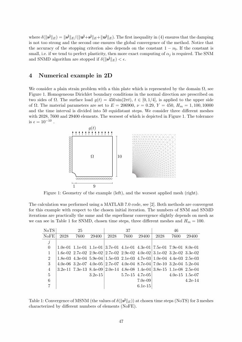
where δ(∥sj∥E) = ∥sj∥E/(∥uj+sj∥E+∥uj∥E). The first inequality in (4) ensures that the dampingis not too strong and the second one ensures the global convergence of the method. Notice thatthe accuracy of the stopping criterion also depends on the constant 1 − ν0. If the constant issmall, i.e. if we tend to perfect plasticity, then more exact computing of αj is required. The SNMand SNMD algorithm are stopped if δ(∥sj∥E) < ϵ.

4 Numerical example in 2D

We consider a plain strain problem with a thin plate which is represented by the domain Ω, seeFigure 1. Homogeneous Dirichlet boundary conditions in the normal direction are prescribed ontwo sides of Ω. The surface load g(t) = 450 sin(2πt), t ∈ [0, 1/4], is applied to the upper sideof Ω. The material parameters are set to E = 206900, ν = 0.29, Y = 450, Hm = 1, 100, 10000and the time interval is divided into 50 equidistant steps. We consider three different mesheswith 2028, 7600 and 29400 elements. The worsest of which is depicted in Figure 1. The toleranceis ϵ = 10−10 .

cccccccccccccccccc

cccccccccccccccccc

6666666666666

g(t)

Ω

1 9

10

Figure 1: Geometry of the example (left), and the worsest applied mesh (right).

The calculation was performed using a MATLAB 7.0 code, see [2]. Both methods are convergentfor this example with respect to the chosen initial iteration. The numbers of SNM and SNMDiterations are practically the same and the superlinear convergence slightly depends on mesh aswe can see in Table 1 for SNMD, chosen time steps, three different meshes and Hm = 100.

NoTS 25 37 46

NoFE 2028 7600 29400 2028 7600 29400 2028 7600 29400

j0 1.0e-01 1.1e-01 1.1e-01 3.7e-01 4.1e-01 4.3e-01 7.5e-01 7.9e-01 8.0e-011 1.6e-02 2.7e-02 2.9e-02 2.7e-02 2.9e-02 4.0e-02 3.1e-02 3.2e-02 3.3e-022 1.8e-03 4.3e-04 5.9e-04 1.5e-03 2.1e-03 4.7e-03 1.0e-04 4.4e-03 2.5e-033 4.0e-06 3.2e-07 4.0e-05 2.7e-07 4.0e-04 8.7e-04 7.0e-10 3.2e-04 5.2e-044 3.2e-11 7.3e-13 8.4e-09 2.0e-14 4.8e-08 1.4e-04 3.8e-15 1.1e-08 2.5e-045 3.2e-15 5.7e-15 4.7e-05 4.0e-15 1.5e-076 7.0e-09 4.2e-147 6.1e-15

Table 1: Convergence of MSNM (the values of δ(∥sj∥E)) at chosen time steps (NoTS) for 3 meshescharacterized by different numbers of elements (NoFE).

47

For the finest mesh, we test the numbers of regula-falsi iterations in dependence on Hm. We needmaximally 0, 1, 2 regula-falsi iteration for Hm = 10000, 100, 1, respectively. Thus the additionalcomputing of αj is not too costly in this example and SNMD gives the same results as SNM forHm = 10000 since αj = 1.

5 Conclusion

The semismooth Newton methods with and without damping have been used to solve the elasto-plastic problem. The main advantage of SNMD is a global convergence which does not hold forSNM in general. On the other hand, computing of the damping coefficients could not be verycostly. The proposed stopping criterion (4) ensures all the theoretical convergence results ofSNMD and yields good numerical results in combination with the regula-falsi method.

SNMD can also be used for some semicoercive problems where the first inequality in (2) holdsonly for ν0 = 1. It can happened for example for perfect plasticity or some simplified elasto-damage-plastic models, see [4]. SNMD has also been used to solving a semicoercive problem witha beam on a non-linear subsoil, see [6]. In such cases, we must replace 1 − ν0 in the stoppingcriterion (4) by a suitable tolerance parameter.

Acknowledgement: This work has been supported by the Grant Agency of the Czech Republic,contract No. 105/09/1830.

References

[1] R. Blaheta: Numerical methods in elasto-plasticity. Documenta Geonica 1998, PERES Pu-blishers, Prague, 1999.

[2] P. Byczanski, S. Sysala: Modified semismooth Newton method: Numerical example. In: Pro-ceedings of seminar “SiMoNA 2009”, Liberec, 24–30, 2009.

[3] X. Chen, Z. Nashed, L. Qi: Smoothing methods and semismooth methods for nondifferentiableoperator equations. SIAM J. Numer. Anal. 38, 1200–1216, 2000.

[4] E.A.S. Neto, D. Peric, D.R.J. Owen: Computational methods for plasticity: Theory andapplications. Wiley, 2008.

[5] L. Qi, J. Sun: A nonsmooth version of Newton’s method. Mathematical Programming 58,353–367, 1993.

[6] S. Sysala: Numerical modelling of semi-coercive beam problem with unilateral elastic subsoilof Winkler’s type. Appl. Math., 55, 2010, in press.

[7] S. Sysala: Application of the modified semismooth Newton method to some elasto-plasticproblems. Mathematics and Computer in Simulation, Modelling 2009, Submitted.

48

Study of using corners for BDDC in 3D

M. Certıkova, P. Burda, J. Novotny, J. Sıstek

Department of Mathematics, Faculty of Mechanical Engineering andDepartment of Mathematics, Faculty of Civil Engineering

Czech Technical University in PragueInstitute of Mathematics and Institute of Thermomechanics

Academy of Sciences of the Czech Republic, Prague

1 Introduction

Numerical solution of linear problems arising from isotropic elasticity discretized by finite ele-ments is important in many areas of engineering. The matrix of such systems is typically large,sparse, and ill-conditioned. For large problems, iterative methods such as the preconditionedconjugate gradients (PCG) are usually less expensive than direct solvers in terms of memoryand computational time. However, their convergence rate deteriorates with growing conditionnumber of the solved linear system and good preconditioning becomes essential. The need ofefficient preconditioners tailored to the solved problem that can be implemented in parallel gaverise to the field of domain decomposition methods [1].

The Balancing Domain Decomposition by Constraints (BDDC) method [2, 3] is an iterativesubstructuring primal domain decomposition method. The BDDC method is closesly related tothe earlier FETI-DP method. It has been recently proved by Mandel, Dohrmann, and Tezaur[3], that the two methods are spectrally equivalent, which allows for application of numericalresults computed for one method to the other.

In both methods, a fundamental role is played by a coarse space defined by a choice of constraintson continuity. Optimal choice of these constraints has strong influence on convergence of themethod. However, this choice in practice is not a satisfactorily solved problem yet. In this paper,we study the influence of adding more corners (coarse node constraints), on time effectivity ofthe computation. Our tests include both scholastic and industrial 3D linear elasticity problems.

2 The BDDC method

After discretization by the finite element method (FEM), the linear system Ku = f is to besolved for a vector u of unknown values of displacements at nodes of a given domain.

The domain is split into nonoverlapping subdomains with the interface formed by unknownscommon to at least two subdomains. Then the problem is reduced to the Schur complementproblem with respect to the interface and this reduced problem is solved by PCG method. TheBDDC method is used as a preconditioner, that splits the computation of the preconditionedresidual needed in every iteration of PCG to solution of independent subdomain problems andthe global coarse problem. The preconditioned residual is obtained as a combination of theirsolutions (for details see [1, 2, 3]).

The coarse problem is solved on the coarse space, which consists of functions that are continuousacross the interface at selected degrees of freedom only. Functions from the coarse space are fullydetermined by their values at these coarse degrees of freedom and by the requirement of havingminimal energy elsewhere.

49

Choice of the coarse degrees of freedom has great impact on the performance of the preconditio-ner. The simplest choice of coarse degrees of freedom is a function value at a selected node on theinterface. Such node is then called corner. It was shown that while for 2D elasticity problemsthe BDDC (or FETI-DP) preconditioner is scalable for coarse space defined by corners only,in 3D elasticity problems more general coarse degrees of freedom, such as (weighted) averagevalues over edges and faces, need to be used in order to achieve the scalability, see e.g. Toselliand Widlund [1]. In what follows we deal with 3D problems only.

3 The implementation

In every PCG iteration, the following types of problems are to be solved:

• On every subdomain, a local problem with zero Dirichlet boundary condition on the inter-face.

• On every subdomain, a local problem with zero Dirichlet boundary condition on the coarsedegrees of freedom on interface and zero Neumann boundary condition on the rest of theinterface.

• Global coarse problem for coarse degrees of freedom only.

Only values of the boundary conditions, not their type, change from iteration to iteration, so allthe factorizations can be prepared in advance. During the PCG cycle only back-substitutionsare performed.

We implemented BDDC on top of common components of existing finite element codes – thefrontal solver and the element stiffness matrix generation. The coarse problem is solved usingstandard FEM approach with subdomains playing the role of elements. Thus the coarse matrixin not assembled as a whole but stored distributed among processors as local coarse matrices.Lagrange multipliers are used for implementation of the coarse averages. Detailed description ofthe implementation can be found in [5], in less detail it is described also in [4].

4 Numerical results

Presented calculations were performed on 12-36 processors of SGI Altix 4700 computer of Super-computing Centre of Czech Technical University in Prague. The METIS graph partitioner is usedas an automatic tool for other than rectangular decompositions.

First we investigated a typical test problem for 3D elasticity: a cuboid with fixed base loaded bypressure of a weight put on the upper face. The geometry is discretized using 24 000 quadraticelements, which leads to 311 943 unknowns. We tested two typical decompositions of the domain:36 cuboid subdomains obtained by plane sections or 36 subdomains obtained by the graph tool,reffered to as Case A or Case C, respectively. Then we tested three different industrial problemsof different sizes. The first one is a problem of elasticity analysis of a turbine nozzle, throughwhich the steam enters the turbine blades. The geometry is discretized using 2 696 quadraticelements, which leads to 40 254 unknowns. The second one is a problem of elasticity analysisof a hip joint replacement which is loaded by pressure from body weight. This mesh consistsof 33 186 quadratic elements resulting in 544 734 unknowns. Both meshes were divided into36 subdomains by the graph tool. The third problem is a problem of stress analysis of a minereel loaded by its own weight and the weight of of the steel rope. The mesh consisting of

50

problem subdomains vertices edges faces interf. nodes all nodes

Case A 36 12 52 75 17 303 103 981

Case C 36 82 181 144 20 321 103 981

Turbine nozzle 36 6 60 101 2 714 13 418

Hip replacement 36 1 19 78 9 222 181 578

Mine reel 1 024 2 451 1 209 4 164 117 113 579 737

Table 1: Decomposition characteristics of the tested problems.

140 816 quadratic elements and 1 739 211 unknowns was divided into 1 024 subdomains by thegraph tool. Decomposition characteristics of the problems are summarized in Table 1.

We experimented with adding corners to an initial set of corners selected by the algorithmpublished in [6], with or without using also averages over faces and edges.

When only corners were used for the coarse problem, adding more corners to the initial set didnot improved efficiency for small problem of the turbine nozzle, but proved to be beneficial formedium-size problems. Figure 1 left shows results for the turbine nozzle, right for the hip jointreplacement problem (very similar results as for hip replacement were obtained also for bothcuboid problems). There are three time series depicted on every graph: the overall computationaltime, the time consumed by factorization of all subproblems, and the time consumed by PCGiterations. For the large problem of mine reel, corners only were not sufficient for convergence.

When also averages were used, adding more corners to the initial set did not improved efficiencyfor small and medium problems, but proved to be beneficial for the large problem of mine reel.Figure 1 left shows results for the cuboid problem A (very similar results were obtained also forthe cuboid problem C), center the hip joint replacement problem, right the mine reel problem.

5 Conclusion

We investigated time efficiency for different choices of the coarse space in the BDDC method.Our tests indicate that the approach of adding more corners to the ”minimal“ set of cornerscan be beneficial for medium problems (either scholar or industrial problems), when the coarsespace is defined by corners only. If also averages on edges and faces are used as coarse degrees offreedom, the improvement is small or none. For small industrial problem of the turbine nozzle wefound no benefit in adding more corners. On the contrary for the large problem of the mine reel,adding more corners proved to be beneficial for convergence, when averages on edges and facesare used as coarse degrees of freedom (without averages convergence was not achieved). However,for really large problems it seems that some more sofisticated techniques for costruction of thecoarse space should be used.

Acknowledgement: We are grateful to Jan Lestina (Vamet Ltd.) for providing the problems ofturbine nozzle and mine reel for testing. We would also like to thank to Jan Mandel and BedrichSousedık for fruitful discussions about BDDC method. This research has been supported by theCzech Science Foundation under grant GA CR 106/08/0403, by the Grant Agency of the Aca-demy of Sciences of the CR under grant IAA200600801, and by projects MSM 6840770001 andMSM 6840770010. It has also been supported by Institutional Research Plans AV0Z 10190503and AV0Z 20760514.

51

Figure 1: Computational time when using corners only: turbine nozzle problem (left) and hipjoint replacement problem (right).

Figure 2: Computational time for coarse space with averages: cuboid problem A (left), hip jointreplacement problem (center) and mine reel problem (right).

References

[1] A. Toselli, O. Widlund, O.: Domain decomposition methods—algorithms and theory. vol. 34of Springer Series in Computational Mathematics, Springer-Verlag, Berlin, 2005.

[2] C.R. Dohrmann: A preconditioner for substructuring based on constrained energy minimi-zation. SIAM J. Sci. Comput. 25, 246–258, 2003.

[3] J. Mandel, C.R. Dohrmann, R. Tezaur: An algebraic theory for primal and dual substructu-ring methods by constraints. Appl. Numer. Math. 54(2), 167–193, 2005.

[4] J. Sıstek, J. Novotny, P. Burda, M. Certıkova: Implementation of the BDDC method basedon the frontal and multifrontal algorithm. In: Blaheta, R. and Stary, J. (ed.), Proceedings ofSeminar on Numerical Analysis, SNA’09, Ostrava, Czech Republic, February 2–6, Instituteof Geonics AS CR, Ostrava, 105–108, 2009.

[5] J. Sıstek, J. Novotny, J. Mandel, M. Certıkova, P. Burda: , P.: BDDC by a frontal solverand stress computation in a hip joint replacement. Math. Comp. Simul. Available online athttp://dx.doi.org/10.1016/j.matcom.2009.01.002, 2009.

[6] P. Burda, M. Certıkova, J. Novotny, J. Sıstek: On Coarse Space for the BDDC Method In:Blaheta, R. and Stary, J. (ed.), Modelling 2009, Book of Abstracts, Roznov pod Radhostem,Czech Republic, June 22–26, Institute of Geonics AS CR, Ostrava, 78, 2009.

52

An algorithm for 3D contact problems with orthotropic friction

Z. Dostal 1, J. Haslinger 2, T. Kozubek 1, R. Kucera 3

1Department of Applied Mathematics, VSB-TU, Ostrava2Department of Numerical Mathematics, Charles University, Prague

3Department of Mathematics and Descriptive Geometry, VSB-TU, Ostrava

1 Introduction

Contact problems represent a special branch of mechanics of solids whose goal is to find an equi-librium state of deformable bodies being in a mutual contact. Due to non-penetration and frictionconditions, problems we have to solve are highly non-linear. For linearly elastic materials obey-ing a Hook law for small deformations, a linearization of the non-penetration conditions leadsto a convex set of kinematically admissible displacements (geometrical nonlinearity). Anothernon-linearity originates from the presence of friction. In the simplest case with an a-priori givenslip bound (Tresca model), the mathematical model is represented by a variational inequalityof the second kind. This model is however too simple since the non-penetration and frictionphenomena are decoupled. For this reason more realistic models of friction have to be used andthe Coulomb friction law is the classical one. The slip bound prescribed in Tresca model isnow replaced by the product of a coefficient of friction F and the norm of the normal contactforce. The coupling of unilateral and friction conditions leads to the so-called implicit variationalinequality (in terms of displacements) or to a quasivariational inequality (in terms of contactstresses). Due to material or contact surface properties it may happen that the effect of frictionis directionally dependent. A discretization of 3D contact problems with orthotropic Coulombfriction characterized by two coefficients of friction F1 and F2 in two mutually orthogonal di-rections was presented in [4]. The scalable algorithm for this problem was developed in [3] whilethe main ideas may be found in [1].

2 Formulation and algorithm

Let us consider two elastic bodies represented by two non-overlapping domains Ωk ⊂ R3 withthe boundaries ∂Ωk, k = 1, 2. Each boundary consists of three non-empty disjoint parts Γk

u, Γkp,

and Γkc open in ∂Ωk, so that ∂Ωk = Γ

ku ∪ Γ

kp ∪ Γ

kc . The zero displacements are prescribed on Γk

u

while surface tractions act on Γkp. On the contact interface given by Γ1

c and Γ2c we consider

contact conditions: the non-penetration of the bodies, the transmission of the contact stresses,and the effect of orthotropic Coulomb friction. Finally we suppose that each body Ωk is subjectto volume forces.

Our algorithm is based on the fixed-point approach in which the solution to the original problemis defined as a fixed-point of an auxiliary mapping acting on the contact interface. To find fixed-point we use the method of successive approximations whose individual iterative steps are givenby contact problems with orthotropic Tresca model of friction.

The finite element approximation of the auxiliary problems combined with the TFETI domaindecomposition method [2] leads to the following algebraic minimization problem:

53

minimize1

2u⊤Ku− u⊤f +

mc∑i=1

gi∥Fi(T1,iu, T2,iu)⊤∥2, (1)

subject to BEu = 0, Nu ≤ d, (2)

where K = diag(K1, . . . ,Ks) is a symmetric positive semidefinite block-diagonal stiffness matrixof order n, f ∈ Rn is the load vector, BE is an m × n full rank ”gluing”matrix, N denotes anmc×n full rank matrix describing together with d ∈ Rmc the non-penetration condition, T1,i, T2,iare rows ofmc×n full rank matrices T1, T2, respectively, Fi ∈ R2×2 are the value of the coefficientof friction, and gi denote discrete slip bound values at contact nodes.

Even though (1)-(2) is the minimization problem with the unique solution, it is not suitablefor direct numerical solution. The reasons are that K is typically singular, the summation termin (1) is non-differentiable, and the feasible set in (2) is in general so complex that the projectioninto it can hardly be effectively computed. In order to overcome these difficulties, one can applythe duality theory of convex programming [1].

To regularize the non-differentiability we use the following idea based on the Cauchy-Schwarzinequality in R2:

max∥F−1

i λT,i∥2≤gi

(T1,iu, T2,iu)λT,i = gi∥Fi(T1,iu, T2,iu)⊤∥2, (3)

where λT,i ∈ R2 plays the role of Lagrange multipliers. We will denote λT,i = (λT1,i, λT2,i)⊤. It

is easily seen that the constraints on λT,i in (3) are the ellipsoidal inequalities.

In the dual formulation of (1)-(2) we use three types of Lagrange multipliers: λE ∈ Rm

and λN ∈ Rmc are associated with the equality and the inequality constraints in (2), whileλT1 , λT2 ∈ Rmc regularize the non-differentiability via (3). To simplify the notation we denote

λ =

λEλNλT1

λT2

, B =

BE

NT1T2

, c =

0d00

.

The Lagrangian associated with the problem (1)-(2) reads as

L(u, λ) =1

2u⊤Ku− u⊤f + λ⊤(Bu− c), (u, λ) ∈ Rn × Λ(g),

and the set of the Lagrange multipliers is given by

Λ(g) = λ ∈ Rm+3mc : λN,i ≥ 0, ∥F−1i λT,i∥22 ≤ g2i , i = 1, . . . ,mc.

It is well known [1] that (1)-(2) is equivalent to the saddle-point problem that is the problem offinding (u, λ) ∈ Rn × Λ(g) such that

L(u, λ) = minu∈Rn

maxλ∈Λ(g)

L(u, λ).

As L is convex in the first variable, u can be eliminated by

u = K†(f −Bλ) +Rα,

54

where K† ∈ Rn×n is a generalized inverse to K, R ∈ Rn×l is a matrix whose columns span thenull-space KerK, l denotes the defect of K, and α ∈ Rl is an appropriate vector. In advance,

f −B⊤λ ∈ ImK.

Therefore, (1)-(2) leads to the dual problem:

minimize1

2λ⊤Fλ− λ⊤h, subject to λ ∈ Λ(g), Gλ = e,

whereF = BK†B⊤, h = BK†f − c, G = R⊤B, e = R⊤f.

After homogenization, using orthogonal projectors, and penalization, we arrive at the followingproblem:

minimize1

2λ⊤(PFP + ρQ)λ− λ⊤Ph, subject to λ ∈ Λ(g), Gλ = 0, (4)

where ρ > 0 is arbitrary and Q = G⊤(GG⊤)−1G, P = I − Q denote the orthogonal projectorson ImG⊤ and KerG, respectively.

As (4) consists of the minimization of the quadratic objective function subject to separableconvex inequalities and linear equality constraints, we use the recently proposed optimizationalgorithm based on the augmented Lagrangian method [3]. The important property of thisalgorithm is that the number of iterations needed to get a solution with a given accuracy isuniformly bounded (with respect to the scale of the problem) provided that the spectrum ofthe Hessian is confined in a given interval. The assumption on the spectrum is satisfied due toTFETI domain decomposition method.

3 Numerical experiments

We use the algorithm for solving contact problem with Coulomb friction with the geometry asin Figure 1. The upper body is made of steel while the lower one is made of aluminium. Theapplied surface tractions are seen in the figure, the volume forces are neglected. The coefficientof friction is given by Fi = diag(0.3, 0.3) (isotropic case).

Ω1

Ω2

Γ1u

Γ2

u

Γ1

c= Γ

2

c

Figure 1: Geometry of the model problem

55

Each body Ωk, k = 1, 2, is divided into the same number of sub-domains represented by bricksof the same size that are decomposed then into cubes (trilinear finite elements). By H and hwe denote the decomposition parameter (diameter of bricks) and the discretization parameter(diameter of cubes), respectively. We apply the inexact implementation of the algorithm sothat iter are connected iterates of the augmented Lagrangian algorithm and the method ofsuccessive approximations. By nPFP we denote the number of matrix vector multiplications bythe Hessian matrix. Finally, n, nd = m + 3mc, and l is the number of primal unknowns, dualunknowns, and rigid body modes. The results of our experiments are summarized in Table 1,where releff := nPFP/n is the relative efficiency of the solver.

s H/h = 2 H/h = 3 H/h = 4 H/h = 5

4 (324/153/24) (768/276/24) (1500/435/24) (2592/630/24)

10/180 10/269 11/356 11/4700.5556 0.3503 0.2373 0.1813

32 (2592/1527/192) (6144/2889/192) (12000/4683/192) (20736/6909/192)

11/483 11/657 11/665 12/8470.1863 0.1069 0.0554 0.0408

108 (8748/5493/648) (20736/10506/648) (40500/17139/648) (69984/25392/648)

11/636 11/878 13/906 14/10710.0727 0.0423 0.0224 0.0153

256 (20736/13419/1536) (49152/25791/1536) (96000/42195/1536) (165888/62631/1536)

12/737 14/939 15/1173 16/14000.0355 0.01910 0.0122 0.0084

500 (40500/26673/3000) (96000/51408/3000) (187500/84243/3000)(324000/125047/3000)

14/812 15/1039 17/1533 18/17760.0200 0.0108 0.0081 0.0054

a At each position (n/nd/l), iter/nPFP, and releff are displayed

Table 1: Scalability and relative efficiency.

Acknowledgement: This work has been supported by the grant 101/08/0574 of the GrantAgency of the Czech Republic and by the Research Project MSM6198910027 of the CzechMinistry of Education.

References

[1] Z. Dostal: Optimal quadratic programming algorithms: with applications to variationalinequalities. Springer, New York, 2009.

[2] Z. Dostal, D. Horak, R. Kucera: Total FETI - an easier implementable variant of the FETImethod for numerical solution of elliptic PDE. Comm. Num. Meth. Engrg, 22, 1155–1162,2006.

[3] Z. Dostal, R. Kucera: An optimal algorithm for minimization of quadratic functions withbounded spectrum subject to separable convex inequality and linear equality constraints. Sub-mitted to SIAM J. Optimization, (2009).

[4] J. Haslinger, R. Kucera, T. Kozubek: Discretization and numerical realization of contactproblems with orthotropic Coulomb friction. Submitted to SIAM J. Scientific Computing,2009.

56

Preconditioning of FETI-DP using corners on contact interface

Z. Dostal, D. Horak

Department of applied mathematics, FEECS VSB-Technical University Ostrava, Czech Republic

Our research concerns the preconditioning of FETI-based methods for contact problems. Thestandard FETI-DP is based on the decomposition into non-overlapping subdomains, where thecontinuity of the primal solution at crosspoints is implemented directly into the formulationof the primal problem so that one degree of freedom is considered at each crosspoint and thecontinuity of the solution on auxiliary interfaces is enforced by Lagrange multipliers. The dualitytransforms the general inequality into the nonnegativity constraints. After eliminating the cor-ners, the problem reduces to a small, relatively well conditioned strictly convex QP (QuadraticProgramming) problem with simple bound for Lagrange multipliers that is solved iteratively byefficient algorithms that exploit cheap projections and other tools. For semi-coercive problemsthe efficiency of the FETI-DP can be further improved by introducing special projectors onto anauxiliary space related to rigid body modes of floating bodies and preconditioners - lumped andDirichlet’s. Let us mention that the preconditioners can be applied only to the linear part andtheir efficiency is very small. Once the Lagrange multipliers are known, we solve linear problemto find solution for corners. In both phases we need to build the matrix defining so called coarseproblem and to factorize it. The scalability of FETI-DPC based on active set strategies withadditional planning steps was established by Farhat et al. [6] only experimentally. Dostal et al.proved this scalability theoretically. Numerical scalability for FETI–DP algorithm for coerciveproblems was proven theoretically and experimentally in [1]. Later, the result was extended toinclude mortar disctretization [4] and for semicoercive problems [3].

Farhat et al. observed, [5], that the corner nodes on contact interface cause difficulties andrecommended to avoid them. These difficulties can be overcome through the additional condi-tion that preserves the nonpenetration in Lagrange multipliers, and moreover in this way it ispossible to improve rate of convergence. This richer corner mesh results in better convergenceof the method because of better error propagation across the nonlinear interface and in betterpreconditioning of nonlinear steps using standard FETI-DP preconditioners. We showed expe-rimentally that for unpreconditioned and preconditioned FETI–DP using no corners on contactzone the numbers of CG iterations increase much more rapidly with increasing number of subdo-mains along the contact interface in comparison to the case we use corners on the contact zone,when the numbers of CG iterations vary very moderately. The results demonstrate that for agiven decomposition the use of corners always significantly reduces number of CG iterations forboth unpreconditioned and preconditioned systems and this effect is magnified with increasingnumber of subdomains along the contact interface, i.e. with increasing number of corners on thethe contact zone.

Significant modification making from FETI-DP the method of new type is based on definitionof all nodes on the contact zone as the corners, i.e. constraint matrix with inequality conditionsconsiders only corner nodes. This approach enable us the splitting of the problem into a verysmall nonlinear one with corners as unknowns and a linear one with the Lagrange multipliers forequalities. We eliminate the Lagrange multipliers first and the problem reduces to very small,well conditioned strictly convex QP problem with bound for corners that is solved iterativelyby efficient algorithms or by application of duality resulting in dual problem with Lagrangemultipliers for inequalities. Once the corners are known we solve linear problem to find thesolution for Lagrange multipliers for equalities. In both phases we do not need to build any

57

matrix defining the coarse problem and to factorize it. Moreover we can significantly reduce thenumber of CG interations by applying the standard FETI-DP preconditioners in both cases,i.e., by solving the nonlinear problem with corners and the linear one with Lagrange multipliersas unknowns.

We shall give the results of numerical experiments with parallel implementation using Matlaband PETSc that confirm scalability of the algorithm for contact problems.

Acknowledgement: This research has been supported by the grants: GA CR 101/09/P601.

References

[1] Z. Dostal, D. Horak, D. Stefanica: A scalable FETI-DP algorithm for a coercive variationalinequalities. IMACS J. Appl. Numer. Math., Vol. 54, 378–390, 2005.

[2] Z. Dostal, D. Horak, D. Stefanica: An Overview of Scalable FETI-DP Algorithms forVariational Inequalities. Lecture Notes in Comput. Science and Engineering 55, Procee-dings from the 16th Conference on DDM, New York, Springer, 223–230, 2006.

[3] Z. Dostal, D. Horak, D. Stefanica: A Scalable FETI–DP Algorithm for Semi-coerciveVariational Inequality. Computer Methods in Applied Mechanics and Engineering,Vol. 196(8), ISSN 0045-7825, 1369–1379, 2007.

[4] Z. Dostal, D. Horak, D. Stefanica: A scalable FETI-DP algorithm with non-penetration mor-tar conditions on contact interface. Journal of Comp. and Appl. Mathematics, Vol. 231(2),577–591, ISSN:0377-0427, 2009.

[5] P. Avery, G. Rebel, M. Lesoinne, C. Farhat: A numerically scalable dual-primal substructu-ring method for the solution of contact problems - part I: the frictionless case. Comput.Methods Appl. Mech. Engrg., 193, 2403–2426, 2004.

[6] G. Rebel, C. Farhat, M. Lesoinne, P. Avery: A scalable Dual-Primal domain decompositionmethod for the solution of contact problems with friction. 7th U.S. National Congress onComputational Mechanics, 2003.

58

Adaptive hp-FEM on dynamical meshes with application

to a flame propagation problem

L. Dubcova 1,2, P. Solın 1,3

1 Institute of Thermomechanics, Academy of Sciences of the Czech Republic2 Faculty of Mathematics and Physics, Charles University in Prague, Czech Republic

3 Department of Mathematics and Statistics, University of Nevada, Reno

1 Introduction

Flame propagation problems are highly nontrivial from both the modeling and computationalpoints of view. On the computational side, a major difficulty are sharp moving fronts that need tobe resolved accurately at all times in order to capture the process dynamics correctly. Nowadays,most practitioners are still tackling these problems with non-adaptive methods such as finitedifferences (FDM) or non-adaptive low-order finite elements (FEM) [1]. However, extremely fineuniform meshes are usually needed to attain results with sufficient accuracy, which leads toexcessive computing times and memory requirements. One of the first space-time adaptive FEMalgorithms for flame propagation problems, based on first-order FEM appeared recently [3].

In this paper we present the first algorithm that makes it possible to use adaptive hp-FEM [4, 7]for evolutionary PDEs. In Section 2 we presents a low Mach number laminar flame propagationmodel consisting of two coupled nonlinear parabolic differential equations. Section 3 introducesa novel space-time adaptive algorithm based on a combination of the classical Rothe’s methodand the novel multi-mesh hp-FEM [5, 6]. Numerical results are presented in Section 4.

2 Model problem

We consider a freely propagating laminar flame and its response to a heat-absorbing obstaclerepresented by a set of cooled parallel rods with a rectangular cross-section. The mathematicalmodel is based on the assumption that the motion of the fluid is independent from the tempera-ture θ and species concentration Y . Fluid motion in the burner is neglected. The model consistsof a system of two coupled nonlinear parabolic equations for θ and Y ,

∂θ

∂t−∆θ = ω(θ, Y ) in Ω× (0, T0), (1)

∂Y

∂t− 1

Le∆Y = −ω(θ, Y ) in Ω× (0, T0). (2)

Here, the reaction rate ω(θ, Y ) is defined by the Arrhenius law

ω(θ, Y ) =β2

2LeY e

β(θ−1)1+α(θ−1) , (3)

where α is the gas expansion coefficient in a flow with nonconstant density, β the non-dimensionalactivation energy, and Le the Lewis number (ratio of diffusivity of heat and diffusivity of mass).Both θ, 0 ≤ θ ≤ 1 and Y , 0 ≤ Y ≤ 1 are dimensionless and so is the time t.

59

3 Adaptive hp-FEM on dynamical meshes

The adaptive hp-FEM algorithm for time-dependent problems we use is obtained by combiningthe classical Rothe’s method with the novel multimesh hp-FEM [5, 6].

The Rothe’s method provides a better setting for the application of spatially adaptive algorithmscompared to the method of lines (MOL). In every time step, an evolutionary PDE is approxi-mated by means of one or more time-independent ones. The spatial discretization error can becontrolled by solving the time-independent equations adaptively, and the size of the time stepcan be adjusted using standard ODE techniques. In our computations adaptive time integrationis carried out using a pair of first-order backward-difference formulas, whose combination yieldsa second-order scheme [2]. In every time step, the difference between the pair of results providesan estimate of the local error that is used to adapt the time step.

In the (n+1)st time step, the approximations θn(x), Y n(x), that have been obtained in the pre-vious time step, are used as data. Note, however, that they are defined on a locally refined meshthat was created automatically during the nth time step, while the unknowns θn+1(x), Y n+1(x)are solved adaptively starting from a coarser mesh. As a result, the meshes obtained on each timelevel are different, i.e., the mesh changes dynamically in time. In order to keep the algorithms ona reasonable level of complexity, the meshes are not completely unrelated. Each of the meshes Tnis obtained from a very coarse master mesh Tm using sequence of local mutually independentrefinements. In order to evaluate exactly the weak formulation of the coupled problem (1), (2)when the solution pairs θn(x), Y n(x) and θn+1(x), Y n+1(x) are defined on different meshes, weuse the multi-mesh hp-FEM [5, 6]. In this technology the stiffness matrix is assembled on a vir-tual union mesh Tu which is the geometrical union of the meshes Tn and Tn+1, as illustratedin Fig. 1. In this way, no additional error arises since no transfer of information between themeshes takes place.

Figure 1: Example of a master mesh Tm, meshes Tn, Tn+1 and the union mesh Tu.

The final space-time adaptive algorithm can be summarized as follows:

1. calculate a temporal error estimate ek = ||ω(θ1, Y1)− ω(θ2, Y2)||L2

2. calculate a spatial error estimate eh = ||ω(θ1, Y1)− ω(θ, Y )||H1/||ω(θ, Y )||H1

3. if both ek < TIMETOL and eh < SPACETOL, perform mesh coarsening and proceed tothe next time level with new time step

4. else

• if ek > TIMETOL adjust time step τk = τk

√TIMETOL

ek

• if eh > SPACETOL perform mesh adaptation

and repeat process.

60

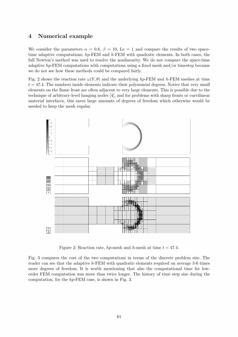
4 Numerical example

We consider the parameters α = 0.8, β = 10, Le = 1 and compare the results of two space-time adaptive computations; hp-FEM and h-FEM with quadratic elements. In both cases, thefull Newton’s method was used to resolve the nonlinearity. We do not compare the space-timeadaptive hp-FEM computations with computations using a fixed mesh and/or timestep becausewe do not see how these methods could be compared fairly.

Fig. 2 shows the reaction rate ω(Y, θ) and the underlying hp-FEM and h-FEM meshes at timet = 47.4. The numbers inside elements indicate their polynomial degrees. Notice that very smallelements on the flame front are often adjacent to very large elements. This is possible due to thetechnique of arbitrary-level hanging nodes [4], and for problems with sharp fronts or curvilinearmaterial interfaces, this saves large amounts of degrees of freedom which otherwise would beneeded to keep the mesh regular.

Figure 2: Reaction rate, hp-mesh and h-mesh at time t = 47.4.

Fig. 3 compares the cost of the two computations in terms of the discrete problem size. Thereader can see that the adaptive h-FEM with quadratic elements required on average 5-6 timesmore degrees of freedom. It is worth mentioning that also the computational time for low-order FEM computation was more than twice longer. The history of time step size during thecomputation, for the hp-FEM case, is shown in Fig. 3.

61

0

5000

10000

15000

20000

25000

30000

35000

40000

0 10 20 30 40 50 60

DO

Fs

Time

hp-adaptivity h-adaptivity

Figure 3: Comparison of discrete problem size as a function of time (left) and the size of timestep during the computation (right).

5 Conclusion

We presented a novel PDE-independent space-time adaptive hp-FEM algorithm for evolutionaryproblems based on a combination of the Rothe’s method with a novel adaptive multi-meshhp-FEM technique. The method was applied to solve a low Mach number flame propagationmodel consisting of a pair of coupled nonlinear parabolic PDEs. The method was tested withfavorable results against space-time adaptive FEM with low-order (quadratic) elements. Thealgorithms described in this paper are freely available under the GPL license as part of themodular higher-order finite element C++ library Hermes.

References

[1] R.C. Aldredge: Turbulent flame propagation with large chemical-heat release. In: AppliedMathematical Modelling, in press, September 2008.

[2] J. Hoffman, C. Johnson: Adaptive finite element methods for incompressible fluid flow. In:T. Barth, H. Deconinck (eds.), 97–157, 2003.

[3] M. Schmich, B. Vexler: Adaptivity with dynamical meshes for space-time finite elementdiscretizations of parabolic equations. In: SIAM J. Sci. Comput. Vol. 30 (1), 369–393, 2008.

[4] P. Solin, J. Cerveny, I. Dolezel: Arbitrary-level hanging nodes and automatic adaptivity inthe hp-FEM. In: Math. Comput. Simul 77, 117–132, 2008.

[5] P. Solin, J. Cerveny, L. Dubcova, D. Andrs: Monolithic discretization of linear thermo-elasticity problems via adaptive multimesh hp-FEM. In: J. Comput. Appl. Math, 2009, doi10.1016/j.cam.2009.08.092.

[6] P. Solin, L. Dubcova, J. Kruis: Adaptive hp-FEM with dynamical meshes for tran-sient heat and moisture transfer problems. In: J. Comput. Appl. Math, 2009, doi10.1016/j.cam.2009.07.025.

[7] P. Solin, K. Segeth, I. Dolezel: Higher-order finite element methods. Chapman & Hall/CRCPress, 2003.

62

On the Ritz values that can be generated

by the Arnoldi method

J. Duintjer Tebbens, G. Meurant

Institute of Computer Science, Academy of Sciences of the Czech Republic, Prague

1 Introduction

The Arnoldi method generates approximate eigenvalues of a complex n× n matrix A by consi-dering a starting unit vector v ∈ Cn and a decomposition

AVk = VkHk, Vke1 = v,

where V ∗k Vk = I and Hk is upper Hessenberg with a positive real lower sub-diagonal. The

approximate eigenvalues found in the kth iteration of the Arnoldi method, called Ritz values,are the eigenvalues of Hk. In case A is Hermitian, the method generates a matrix Hk which istridiagonal and the method is called Lanczos method.

In his 1979 paper, Scott showed that the Lanczos method may converge very slowly in pathologiccases [4]. More precisely, given a Hermitian positive definite matrix A with the eigenvalues

λ1 < λ2 < · · · < λn,

he constructed a perverse starting vector v such that the eigenvalues of Hn−1 are

λ1 + λ22

,λ2 + λ3

2, . . . ,

λn−1 + λn2

.

That is, convergence may be postponed until the very last iteration.

This extended abstract deals with generalizations of Scott’s result to the Arnoldi algorithm. Inthe case where A is normal but not Hermitian, we can easily exploit a procedure due to Ericssonto obtain the desired generalization. It turns out that in the next to last iteration one maygenerate any distribution of Ritz values as long as it satisfies a generalized interlacing propertywith respect to the spectrum of A. This is done in the next section. The last section presentsfurther generalization for non-normal, diagonalisable matrices and discusses several other issuesrelated to generating prescribed Ritz values in the Arnoldi method.

2 The normal case

The procedure described on page 10 of [1] leads to a method to compute a normal upperHessenberg matrix H ∈ Cn×n with given distinct eigenvalues and given spectrum of its leadingprincipal submatrix. This spectrum, µ1, . . . , µn−1, must satisfy what is called a generalized inter-lacing property in [1], namely

Π(r) ≡∏n−1

j=1 (λr − µj)∏nj=1,j =r(λr − λj)

> 0, 1 ≤ r ≤ n, (1)

where λ1, . . . , λn are the distinct eigenvalues of H.

63

The following theorem shows how the procedure on page 10 of [1] can be used to construct fora given normal matrix with distinct eigenvalues an initial Arnoldi vector such that the Arnoldimethod applied to the normal matrix with the initial Arnoldi vector yields prescribed Ritz valuesin the next to last step.

Theorem. Consider a normal matrix A with spectral decomposition A =Wdiag (λ1, . . . , λn)WH

where the eigenvalues λ1, . . . , λn are distinct and consider n−1 values µi such that the generalizedinterlacing property (1) is satisfied. Let z ∈ Cn be any vector satisfying

|zr|2 = Π(r), 1 ≤ r ≤ n,

and letΛZ = ZH

be the Arnoldi decomposition generated by the matrix Λ = diag (λ1, . . . , λn) and initial vectorZe1 = z, i.e. ZHZ = I and H is upper Hessenberg with a positive real lower subdiagonal. Thenthe Arnoldi algorithm applied to A with initial vector

v ≡WZen

generates in the (n− 1)st iteration the Ritz values µ1, . . . , µn−1.

P r o o f : Let H be an upper Hessenberg matrix with eigenvalues (λ1, . . . , λn) and leadingprincipal submatrix whose spectrum consists of the values µ1, . . . , µn−1. Let HX = XΛ be thespectral decomposition of H. Paige showed in [2] that

|Xn,r|2 = Π(r), 1 ≤ r ≤ n,

see also [3, 1, 5]. Hence there holds Xn,r = eiϕrzr for values ϕr, 0 ≤ ϕr ≤ 2π, and for 1 ≤ r ≤ n.If D = diag (ϕ1, . . . , ϕn) this means that we have

XT en = Dz. (2)

Let P = (en, . . . , e1) be the permutation matrix containing the columns of the identity matrixin reversed order and let H be the upper Hessenberg matrix defined by H ≡ PHTP . Then fromHX = XΛ we have

ΛXTP = XTPH.

This is an Arnoldi decomposition generated by the matrix Λ and initial vectorXTPe1 = XT en =Dz. On the other hand, from ΛZ = ZH we obtain

DΛZ = ΛDZ = DZH,

i.e. an Arnoldi decomposition generated by the matrix Λ and initial vectorDZe1 = Dz. It followsfrom the uniqueness of the Arnoldi decomposition that the two decompositions are identical andH = H. Then we obtain from ΛZ = ZH, subsequently,

ΛZP = ZPPHP = ZPHT ,

PZTΛ = HPZT ,

PZTWHWΛWH = HPZTWH ,

AW (PZT )H =W (PZT )HH.

BecauseW (PZT )H is unitary, the last equation represents the Arnoldi decomposition generatedby the matrix A and initial vectorWZPe1 =WZen. Its Hessenberg matrix has the desired Ritzvalues.

64

3 Further generalizations

The previous theorem can be generalized to the case where A is diagonisable but not necessarilynormal. The eigenvalues must be distinct and the Ritz values must satisfy a modification of (1).

Theorem. Let A be diagonalisable with spectral decomposition A = Wdiag (λ1, . . . , λn)W−1

where the eigenvalues λ1, . . . , λn are distinct and consider n−1 values µi such that the nonlinearsystem of equations in the complex variables z1, . . . , zn,

diag(z1, . . . , zn)(WHW )−1z =

Π(1)

. . .

Π(n)

(3)

has a solution. Let z ∈ Cn be any vector satisfying (3) and let

ΛZ = ZH

be the (WHW )−1-orthogonal Arnoldi decomposition generated by the complex conjugate of thematrix Λ = diag (λ1, . . . , λn) and initial vector Ze1 = z, i.e. ZH(WHW )−1Z = I and H isupper Hessenberg with a positive real lower subdiagonal. Then the Arnoldi algorithm applied toA with initial vector

v ≡WZ−Hen

generates in the (n− 1)st iteration the Ritz values µ1, . . . , µn−1.

In our talk we plan to address the proof of this theorem and the geometric meaning of theinterlacing properties (1) and (3). We also envisage to discuss generating prescribed Ritz values inarbitrary iteration numbers smaller than n−1. Finally, we will mention the problem of generatingprescribed Ritz values when A is not given but, as the starting vector v, is constructed. In thiscase it is possible to prescribe the Ritz values of more than one iteration number.

Acknowledgements: The authors thank Zdenek Strakos for initiating work on this topic. Thework of the first author was supported by project number KJB100300703 of the Grant Agencyof the Academy of Sciences of the Czech Republic.

References

[1] T. Ericsson: On the eigenvalues and eigenvectors of Hessenberg matrices. Technical report,1990.

[2] C.C. Paige: The Computation of Eigenvalues and Eigenvectors of Very Large Sparse Matri-ces. Ph.D. Thesis, University of London, 1971.

[3] B.N. Parlett: The symmetric eigenvalue problem. Prentice-Hall Inc., Englewood Cliffs, N.J.,1980. Prentice-Hall Series in Computational Mathematics.

[4] D.S. Scott: How to make the Lanczos algorithm converge slowly. Math. Comp., 33(145),239–247, 1979.

[5] J.-P.M. Zemke: Hessenberg eigenvalue-eigenmatrix relations. Linear Algebra Appl., 414(2-3),589–606, 2006.

65

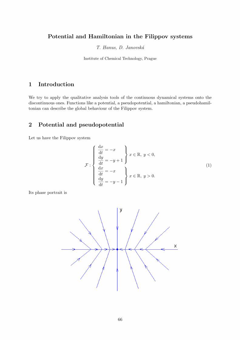
Potential and Hamiltonian in the Filippov systems

T. Hanus, D. Janovska

Institute of Chemical Technology, Prague

1 Introduction

We try to apply the qualitative analysis tools of the continuous dynamical systems onto thediscontinuous ones. Functions like a potential, a pseudopotential, a hamiltonian, a pseudohamil-tonian can describe the global behaviour of the Filippov system.

2 Potential and pseudopotential

Let us have the Filippov system

F :

dx

dt= −x

dy

dt= −y + 1

x ∈ R, y < 0,

dx

dt= −x

dy

dt= −y − 1

x ∈ R, y > 0.

(1)

Its phase portrait is

66

The function

U(x, y) =

−1

2x2 − 1

2(y − 1)2, x ∈ R, y < 0,

−1

2x2 − 1

2(y + 1)2, x ∈ R, y ≥ 0,

(2)

is the potential of the system (1). We can see that the gradient of (2) is equal to the vector fieldof (1) in all points, except for those with y = 0:[

∂U

∂x,∂U

∂y

]=

[−x,−y + 1] , x ∈ R, y < 0,

[−x,−y − 1] , x ∈ R, y > 0.

The function

U(x, y) = (−2) · U(x, y) =

x2 + (y − 1)2, x ∈ R, y < 0,

x2 + (y + 1)2, x ∈ R, y ≥ 0,(3)

is the pseudopotential of the system (1). The fall lines of (3) projected into the plane xy are thetrajectories of (1).

3 Hamiltonian and pseudohamiltonian

Now, let us have the Filippov system

F :

dx

dt= −y + 1

dy

dt= x

x ∈ R, y < 0,

dx

dt= −y − 1

dy

dt= x

x ∈ R, y > 0,

(4)

with its phase portrait

67

The function

H(x, y) =

−1

2x2 − 1

2(y − 1)2, x ∈ R, y < 0,

−1

2x2 − 1

2(y + 1)2, x ∈ R, y ≥ 0.

(5)

is the hamiltonian of the system (4). We can notice, that the condition[∂H

∂y,−∂H

∂x

]=

[−y + 1, x] , x ∈ R, y < 0,

[−y − 1, x] , x ∈ R, y > 0,

holds for all points, except for those with y = 0. So the gradient of (5) is always orthogonal tothe vector field of (4).

The function

H(x, y) = (−2) ·H(x, y) =

x2 + (y − 1)2, x ∈ R, y < 0,

x2 + (y + 1)2, x ∈ R, y ≥ 0.(6)

is the pseudohamiltonian of the system (4). The level curves of (6) are the trajectories of (1)free of orientation.

4 Graph

Here we have 3D graph of (3) and (6). They happened to be the same, which is not the rule, ofcourse.

It is a function of two variables, continuous, but not smooth. It is not differentiable at the pointswith y = 0.

68

5 Conclusion

A discontinuous dynamical system is defined piecewise, there is a special formula on each sub-domain of the state space. Handling such system requires switching formulas on the boundarybetween the subdomains. This work is the first step of the long journey. Once we will haveone formula of a dynamical system on the entire state space no matter if it is continuous ordiscontinuous.

Acknowledgement: This work has been supported by the grant MSM 6046137306.

References

[1] A. F. Filippov: Differencial’nyje uravnenija s razryvnoj pravoj cast’ju. Nauka, Moskva, 1985.

[2] M. W. Hirsch, S. Smale, R. L. Devaney: Differential equations, dynamical systems, and anintroduction to chaos. Elsevier Academic Press, USA, 2004.

[3] A. Klıc, M. Kubıcek: Matematika III, Diferencialnı rovnice. VSCHT, Praha, 1992.

[4] Y. A. Kuznetsov, S. Rinaldi, A. Gragnani: One-parameter Bifurcations in Planar FilippovSystems. In: Int. J. Bifurcation and Chaos, 2003, 2157–2188.

69

Redukce diskretnı puklinove sıte a jejı vliv

na resenı ulohy proudenı

J. Havlıcek, M. Hokr, J. Kopal, P. Ralek

Fakulta mechatroniky, informatiky a mezioborovych studiı

Technicka univerzita v Liberci

1 Uvod

Prıspevek se venuje popisu vlastnostı algoritmu pro redukci dvourozmerne puklinove sıte a vlivteto redukce na resenı ulohy proudenı v diskretnı puklinove sıti s mechanickym zatızenım.Problem vznikl jako soucast projektu Decovalex-2011, Task C [1].

Potreba redukovat rozsahlou puklinovou sıt’ tak, aby zustaly priblizne zachovany jejı hydraulickevlastnosti (nebo abychom tuto zmenu umeli vysledovat), vznikla pri snaze implementovat sdruze-nou ulohu proudenı–mechanika. Vliv mechanickeho zatızenı na rozevrenı pukliny je v soucasnedobe pocıtan analyticky zvlast’ pro kazdou puklinu, nicmene vznikly reduktor sıte poskytujezajımave poznatky o vlastnostech puklinove sıte, kdy velkou roli z hlediska toku oblastı hrajemaly pocet velkych puklin.

2 Popis ulohy

Modelovanou oblastı je ctverec o delce strany 20m, na kterem je stochasticky generovana dis-kretnı puklinova sıt’ (s parametry podle realnych merenı [2], [3]). Rozevrenı puklin je umernejejich delce. Pro ulohu proudenı je zadana Dirichletova okrajova podmınka pro tlakovou vyskua gradient tlaku (dve ruzne okrajove podmınky jsou znazorneny na obr. 1 vlevo a vpravo).Podrobnemu popisu numerickeho resenı ulohy proudenı (bez zahrnutı mechanickeho zatızenı)za pouzitı programu Flow123D se venuje [5].

Obrazek 1: Okrajove podmınky pro proudenı a mechaniku.

Pro mechaniku jsou zadana horizontalnı a vertikalnı napetı (viz obr. 1 uprostred). Pri pusobıcımmechanickem napetı nektere pukliny zmensı svoje rozevrenı a jejich hydraulicka vodivost po-klesne. U vhodne orientovanych puklin vuci vnejsımu napetı dochazı ke zvetsenı rozevrenı a hyd-raulicka vodivost roste. Mechanicky model puklin (vzorce pro analyticky vypocet napetı, defor-mace, tuhost puklin, pevnostnı kriteria) byl prevzat z [3]. Podprobnemu popisu vlivu mechanikyna hydraulicke vlastnosti puklinove sıte se venuje [6].

70

3 Redukce puklinove sıte

Kvuli prılis velke hustote puklinove sıte vznikl pozadavek na jejı redukci pri pribliznem zachovanıhydraulickych vlastnostı tak, abychom na ridsı sıti jiz mohli resit slozitejsı ulohu nez prosteproudenı (proudenı–mechanika, zahrnutı transportu castic). Pro redukci puklinove sıte (tzn.snızenı poctu puklin a jejich prusecıku – uzlu) lze pouzıt nekolik postupu.

• Vymazanı (volitelne) malych puklin: u dostatecne malych puklin lze predpokladat, ze jejichvliv na celkove proudenı bude maly (rozevrenı puklin je umerne jejich delce).

• Vymazanı slepych useku puklin: casti puklin mezi poslednım prusecıkem (uzlem) s jinoupuklinou a koncem pukliny nemajı vliv na ustalene proudenı v puklinove sıti.

• Slucovanı (volitelne) blızkych uzlu (obr. 2): cılem je snızit celkovy pocet prusecıku puklin.Slucujı se vzdy dva uzly lezıcı na teze pukline, zustane tak zachovana sousednost v pukli-nove sıti. Slucovanım uzlu lze odstranit miniaturnı useky puklin a zlepsit pomer mezinejmensım a nejvetsım elementem v diskretizaci.

• Slucovanı soubeznych useku puklin (obr. 3): v ramci slucovanı uzlu dochazı ke sloucenıcelych useku puklin. V danem useku se sectou rozevrenı slucovanych puklin a vodivost seprepocte z vodivostı slucovanych puklin tak, aby byl zachovan tok puklinou.

Obrazek 2: Ukazka slucovanı uzlu.

Obrazek 3: Princip slucovanı useku puklin.

Uvedene postupy lze ruzne kombinovat. Geometricke a hydraulicke vlastnosti vysledne sıtezavisejı na zvolenych parametrech redukce (ty mohou byt bud’ robustnı nebo jemne). Stejnetak je mozne ovlivnit vysledek redukce preferencı dominantnıch puklin, ktere by nemely bytprubehem redukce ovlivneny. Na obr. 4 je vyrez casti sıte pred a po redukci. Zretelne jsou dvedominantnı pukliny, ktere se pri redukci nemenı.

71

Obrazek 4: Ukazka casti redukovane sıte.

Obrazek 5: Zavislost vystupnıho toku (vlevo) a velikosti ulohy (vpravo) na velikosti vymazanychpuklin.

4 Ukazky vysledku vypoctu

Byla provedena sada vypoctu s ruznymi parametry redukce, bez zahrnutı vlivu mechanickehozatızenı i s nım (vertikalnı napetı je 5 MPa a horizontalnı napetı 5 Mpa nebo 25 MPa). Vysledkyprezentovane zde v abstraktu jsou pro okrajove podmınky znazornene na obr. 1 vpravo, sledovanbyl vystupnı tok dolnı castı hranice oblasti (podle predpokladu pri zvysujıcım se horizontalnımzatızenı celkovy vertikalnı tok klesa). Graf na obr. 5 vlevo popisuje zmenu vystupnıho tokuhranicemi oblasti v zavislosti na mnozstvı vymazanych malych puklin. Pukliny do velikosti 1movlivnujı celkovy vystupnı tok jen velmi malo. Velikost ulohy vsak klesne vyznamnym zpusobem(obr. 5 vpravo). Slucovanım uzlu a soubeznych puklin lze dosahnout dalsıho snızenı velikostiulohy (napr. pro sıt’ s vynechanymi puklinami kratsımi nez 1m s parametrem slucovanı 0.4 metruo cca polovinu), zde vsak jiz hraje velkou roli vliv mechaniky. V uloze proudenı bez zahrnutımechaniky je vliv slucovanı uzlu a soubeznych puklin maly (zmena toku je mensı nez 10%),pri zahrnutı mechaniky je tento vliv narust hydraulicke vodivosti puklin mnohem vyssı, nezodpovıda narustu vodivosti na neredukovane sıti. Krome toho, ze dochazı ke zmene geometriesıte, to muze byt zpusobeno tım, ze pri redukci vznika mensı pocet mnohem sirsıch puklin, proktere je jiz pouzity mechanicky model nepresny.

72

5 Zaver

Testovacı ulohy ukazaly, ze lze vyraznym zpusobem snızit velikost puklinove sıte, aniz to (provhodne zvolene parametry redukce) vyrazne ovlivnı vyslednou bilanci toku hranicı oblasti. Zvo-lit spravne vyvazene parametry redukce nenı snadne a je treba pokazde testovat, nakolik zmenasıte ovlivnı vysledne toky. Pro ulohy se zahrnutım mechaniky jiz dochazı k velke odchylce vevysledcıch oproti tokum na neredukovane sıti. Tomu lze castecne predejıt spocıtanım vlivu me-chanickeho zatızenı na dominantnı pukliny na neredukovane sıti a pote provest redukci.

Redukovane sıti s podobnymi hydraulickymi vlastnostmi jako sıt’ neredukovana by mela v bu-doucnu umoznit slozitejsı vypocty, napr. zahrnutı transportu ci slozitejsıch mechanickych modelupukliny, nez na neredukovane sıti. Vyvstava uloha nalezt zpusob, jak menit materialove parame-try sıte (napr. permeabilitu) tak, aby vysledne toky hranicemi na redukovane sıti byly shodne(ve vetsı mıre nez nynı) s toky na sıti neredukovane.

Acknowledgement: Tento prıspevek vznikl za podpory MPO CR, projekt FR-TI1/362, a v ramciucasti na mezinarodnım projektu Decovalex.

Reference

[1] J.A. Hudson, I. Neretnieks, L. Jing: DECOVALEX-2011 project, Technical Definition ofthe 2-D BMT Problem for Task C. May 2008.

[2] A. Baghbanan, L. Jing: Hydraulic properties of fractured rock masses with correlatedfracture, length and aperture. In: International Journal of Rock Mechanics and MiningSciences, 44(5), 704-719, 2007.

[3] A. Baghbanan, L. Jing: Stress effects on permeability in fractured rock mass with correla-ted, fracture length and aperture. In: International Journal of Rock Mechanics and MiningSciences, 45(8), 1320-1334, 2008.

[4] B. Mala: Fracture net. In: Technical Report TUL, June 2008.

[5] M. Hokr, J. Kopal, J. Havlıcek: Resenı ulohy proudenı v rozsahle diskretnı sıti puklin v kon-textu sdruzenych uloh proudenı-mechanika. In: Sbornık SNA 2009.

[6] M. Hokr, J. Havlıcek: Zmena hydraulickych parametru v modelu proudenı diskretnı pukli-novou sıtı pri zahrnutı vlivu mechaniky. In: Sbornık SIMONA 2009, 45-51.

[7] P. Ralek: Algoritmus pro redukci puklinove sıte v uloze 2D proudenı. In: Sbornık SIMONA2009, 104-110.

73

Two-sided quaternionic polynomials

D. Janovska, G. Opfer

Institute of Chemical Technology, Prague

University of Hamburg, Hamburg

1 Introduction

A general, quaternionic polynomial consists of a sum of terms of the type

tj(z) := a0j · z · a1j · · · aj−1,j · z · ajj , z, a0j , a1j , . . . , ajj ∈ H, j ≥ 0.

We call this term a monomial of degree j. Since there may be several terms of the same degreewe have to enumerate the terms. We do that in the form

tjk(z) := a(k)0j · z · a(k)1j · · · a(k)j−1,j · z · a

(k)jj , k = 1, 2, . . . , kj , kj ≥ 0.

The case kj = 0 means that there is no monomial of degree j. A general, quaternionic polynomialof degree n takes the form

p(z) :=

n∑j=0

kj∑k=1

tjk(z). (1)

We will treat quaternionic polynomials of the two-sided type

p(z) :=n∑

j=0

ajzjbj , z, aj , bj ∈ H, a0b0 = 0, anbn = 0, (2)

where H is the skew field of quaternions. These polynomials include also the one-sided polyno-mials, where all coefficients are located on the left or on the right side of the powers, see [4].

By R, C we denote the fields of real and complex numbers, respectively. By H we denote theskew field of quaternions that consists of elements of R4, equipped with the multiplication rule

ab := (a1b1 − a2b2 − a3b3 − a4b4, a1b2 + a2b1 + a3b4 − a4b3, (3)

a1b3 − a2b4 + a3b1 + a4b2, a1b4 + a2b3 − a3b2 + a4b1),

where a := (a1, a2, a3, a4), b := (b1, b2, b3, b4), aj , bj ∈ R, j = 1, 2, 3, 4.

The multiplication rule implies, in particular,

ℜ(ab) = ℜ(ba) and ra = ar for a, b ∈ H, r ∈ R. (4)

By 1, i, j, k we denote the standard units in H. Two quaternions a, b ∈ H are called equivalent ,if there is an h ∈ H \ 0 such that b = h−1ah. Equivalent quaternions a, b will be denoted bya ∼ b. The set

[a] :=u ∈ H : u = h−1ah for all h ∈ H \ 0

(5)

will be called an equivalence class of a.

74

Equivalent quaternions a, b can be easily recognized by

a ∼ b ⇔ ℜa = ℜb and |a| = |b|, see [3], (6)

where ℜa denotes the real part , the first component of a, and |a| denotes the absolute valueof a = (a1, a2, a3, a4), |a| :=

√a21 + a22 + a23 + a24 . We also introduce ℑa, the imaginary part ,

the second component of a. Let a be real. Then [a] = a, which means, that in this case, theequivalence class consists only of one element, a. If a is not real, then [a] always containsinfinitely many elements,

[a] := z ∈ H : ℜz = ℜa, |z| = |a|, (7)

which may be regarded as the surface of a ball in R3. Let z ∈ H be not real and z = (z1, z2, z3, z4).Then [z] contains exactly two complex numbers, a ∈ C and a ∈ C where a is determined byℜa = z1 and ℑa = +

√z22 + z23 + z24 > 0. The complex number a will be called the complex

representative of [z].

All powers zj , j ∈ N, of a quaternion z have the form zj = αz + β with real α, β, see [6], [4]. Inorder to determine the numbers α, β we set up the following iterations, see [4],

zj = αjz + βj , αj , βj ∈ R, j = 0, 1, . . . , where (8)

α0 = 0, β0 = 1,

αj+1 = 2ℜz αj + βj ,

βj+1 = −|z|2αj , j = 0, 1, . . .

2 Types of zeros of two-sided polynomials

Let z ∈ R be a real zero of p, defined in (1). Since a real z commutes with all quaternions thepolynomial can be written in the form

p(z) =

n∑j=0

Ajzj where Aj :=

kj∑k=1

a(k)0j a

(k)1j · · · a(k)jj , z ∈ R, (9)

i.e. as an one-sided quaternionic polynomial, see [4]. We will skip the discussion on real zeros inthe sequel.

By means of (8), the polynomial p can be written as

p(z) =n∑

j=0

ajzjbj =

n∑j=0

aj(αjz + βj)bj =n∑

j=0

αjajzbj +n∑

j=0

βjajbj = C(z) +B(z), (10)

where C(z) =

n∑j=0

αjajzbj , B(z) =

n∑j=0

βjajbj . (11)

Let C be defined as in (11). Then, C : R4 → R4 is a linear mapping over R. Let z0 be nonreal.Then, B(z), defined in (11), is constant for z ∈ [z0]. If p(z) = 0 for some z ∈ H, then C(z) =B(z) = 0 or C(z) = 0 and B(z) = 0. For details, see [5].

We introduce two mappings τ1, τ2 : H → R4×4 by

τ1(a) :=

a1 −a2 −a3 −a4a2 a1 −a4 a3a3 a4 a1 −a2a4 −a3 a2 a1

∈ R4×4, τ2(a) :=

a1 −a2 −a3 −a4a2 a1 a4 −a3a3 −a4 a1 a2a4 a3 −a2 a1

∈ R4×4. (12)

75

The first mapping τ1 represents the isomorphic image of a quaternion a = (a1, a2, a3, a4) in thematrix space R4×4. Thus, we have τ1(ab) = τ1(a)τ1(b). The two matrices τ1(a), τ2(b) coincide ifand only if a = b ∈ R, see [2]. The second mapping τ2, see [1], has the remarkable property thatit reverses the multiplication order

τ2(ab) = τ2(b)τ2(a).

From the definition (12) it follows that

τ1(a)T = τ1(a), τ2(b)

T = τ1(b).

Both matrices are orthogonal in the sense τ1(a)τ1(a)T = τ1(a)τ1(a) = |a|2 I, τ2(b)τ2(b)T = |b|2 I,

where I is the (4× 4) identity matrix.

Let a := (a1, a2, a3, a4) ∈ H. We introduce an column operator col : H → R4 by

col(a) :=

a1a2a3a4

.

This column operator enables us to regard a quaternion as a matrix with one column and fourrows. It is linear over R, i. e.

col(αa+ βb) = αcol(a) + βcol(b), a, b ∈ H, α, β ∈ R.

For arbitrary quaternions a, b, c we have

col(ab) = τ1(a)col(b) = τ2(b)col(a),

col(abc) = τ1(a)τ2(c)col(b).

For more properties of these mappings, see [5].

Theorem Let p(z) := C(z) +B(z) be defined as in (10), (11). Then,

col(p(z)) =

n∑j=0

αjτ1(aj)τ2(bj)

col(z) +n∑

j=0

βjcol(ajbj) (13)

=: A(z)col(z) + col(B(z)), where (14)

A(z) :=

n∑j=0

αjτ1(aj)τ2(bj)

∈ R4×4, col(B(z)) :=n∑

j=0

βjcol(ajbj). (15)

Instead of considering the equation p(z) = 0 we consider the equivalent equation

P (z) := col(p(z)) = A(z)col(z) + col(B(z)) = col(0) :=

0000

=: 0. (16)

From this formula we obtain: Let z be a nonreal zero of p such that equation (16) is valid.Then, this equation remains valid if in A(z), B(z) the zero z is replaced with the complexrepresentative z0 of [z]. In order to find the nonreal zeros z ∈ H of p, defined in (2), it issufficient to find the complex representative z0 of [z], where, in general, z0 is not a zero of p.The matrix A(z), occurring in (16) may be singular or non singular.

76

From these results we obtain the classification of the zeros of p as follows: Let z be a zero of p,defined in (2), and let z0 ∈ [z] be the complex representative of [z]. We classify the zeros z of pwith respect to the rank of A(z0). The zero z is called zero of type k if rank(A(z0)) = 4 − k,0 ≤ k ≤ 4. A zero of type 4 (rank(A(z0)) = 0) is called spherical zero. It has the property that allz ∈ [z0] are zeros. A zero of type 0 is called isolated zero. In this case z = −(A(z0))

−1col (B(z0))is the only zero in [z0]. We also call a real zero an isolated zero.

Since the polynomial p(z) := z2 + 1 has already infinitely many zeros in H, it makes no senseto count the individual zeros. Let p be any quaternionic polynomial of degree n ≥ 2. By #Z(p)we understand the number of equivalence classes in H which contain zeros of p. We call thisnumber, essential number of zeros of p. Let p be a polynomial of degree n of the form describedin (2). It can be proofed, see [5], that #Z(p), the essential number of zeros of p, is not boundedby n, but it will not exceed 2n.

3 Conclusions

For quaternionic polynomials p of the two-sided type, we have shown that the zeros z may fallinto five different classes, where for each zero the class can be determined by looking at the rankof a (4 × 4) matrix A(z) defined in (16). If a zero in one class has been found, the describedtechnique allows to find all zeros in the same class.

The representation of a given quaternionic, two-sided polynomial p in the form P (z) := A(z)z+B(z) can be used not only for the classification of the zeros, but it can be also successfully appliedto finding the zeros, by applying Newton’s method to P (z) = 0. It shows the typical feature,that it may be slow in the beginning, but it will terminate then very quickly with quadraticrate.

Acknowledgement: The research was supported by the research project MSM 6046137306 ofThe Ministry of Education, Youth and Sports, Czech Republic.

References

[1] L.I. Aramanovitch: Quaternion Non-linear Filter for Estimation of Rotating body Attitude.Mathematical Meth. in the Appl. Sciences, 18, 1239–1255, 1995.

[2] K. Gurlebeck, W. Sprossig: Quaternionic and Clifford Calculus for Physicists and Engi-neers. Wiley, Chichester, 371 p., 1997.

[3] D. Janovska, G. Opfer: Givens’ transformation applied to quaternion valued vectors. BIT,43, 991–1002, 2003.

[4] D. Janovska, G. Opfer: A note on the computation of all zeros of simple quaternionicpolynomials. SIAM J. Numer. Anal., 12 p, 2009, accepted.

[5] D. Janovska, G. Opfer: The classification and the computation of the zeros of quaternionic,two-sided polynomials. Numer. Math., 20 p., 2009, DOI: 10.1007/s00211-009-0274-y.

[6] A. Pogorui, M. Shapiro: On the structure of the set of zeros of quaternionic polynomials.Complex Variables and Elliptic Functions, 49, 379–389, 2004.

77

Stability of non unique solutions

of the Coulomb friction problem

V. Janovsky

Charles University, Faculty of Mathematics and Physics, Prague

1 Discrete static contact problems with Coulomb friction

Let Ω ⊂ R2 be a linearly elastic body supported by a rigid foundation along the contact boun-dary ΓC , see Figure 1. On ΓN and ΓD, Neumann and Dirichlet boundary conditions are prescri-bed. We consider the static contact problems with Coulomb friction, see e.g. [1]. In particular,we will investigate a discrete version of this problem, see e.g. [2]. This may be understood asa FEM-approximation of the continuous mechanical problem:

rigid foundation

Ω

ΓD

ΓN

ΓN

ΓC

Figure 1: 2D elastic body Ω in frictional contact.

Let integers n and p define the degrees of freedom of the body Ω and the number of contactnodes on ΓC , n ≥ 2p. Let f ∈ Rn and F be the given distributed volume force and the frictioncoefficient. We seek for

• distributed displacement field u ∈ Rn,

• distributed normal and tangential stress components λν ∈ Rp and λt ∈ Rp.

First, we formulate the static Tresca friction problem: Given a prescribed slip stress g =(g1, . . . , gp) ∈ Rp

+, find (u,λν ,λt) ∈ Rn ×Λν ×Λt(F ,g), such that

(Au,v)n = (f ,v)n + (λν ,Nv)p + (λt,Tv)p ∀v ∈ Rn, (1)

(µν − λν ,Nu)p + (µt − λt,Tu)p ≥ 0 ∀ (µν ,µt) ∈ Λν ×Λt(F ,g) . (2)

Here, A ∈ Rn×n is a positive definite stiffness matrix. The full-rank matrices N ∈ Rp×n andT ∈ Rp×n represent the actions of the distributed contact forces along the normal and tangentialdirections. The sets

Λν = Rp− , Λt(F ,g) = µt ∈ Rp : |µt,i| ≤ Fgi , ∀ i = 1, . . . , p (3)

are the sets of Lagrange multipliers. Under generic assumptions, the problem (1)&(2) is uniquelysolvable for any data f , F and g.

78

To a given g ∈ Rp+, let us assign the solution (u,λν ,λt) of the problem (1)&(2). In particular,

we consider the map Γ : Rp+ → Rp

+, which is defined as

Γ(g) 7−→ −λν . (4)

The solution (u,λν ,λt) of (1)&(2), which corresponds to the fixed point Γ(g) = −λν = gof the map Γ, is defined as a solution of the static Coulomb friction problem. Under genericassumptions, the fixed point exists for any data f ∈ Rn and F > 0. If F is sufficiently small,the fixed point is unique. In order to find non unique solution of the static Coulomb frictionproblem, path-following technique was proposed, [4, 5].

2 Stability of the fixed point

Let r > 0 be a fixed parameter. The variational inequality (2) is equivalent to the equations

λν = PΛν (λν − rNu) , λt = PΛt(F ,g)(λt − rTu) , (5)

see e.g. [3]. Here, PΛν and PΛt(F ,g) are the orthogonal projections of Rp onto Λν and Λt(F ,g),see (3). Hence, solving (1)&(2) is equivalent to finding roots of nonlinear equations: DefineG : Rp × Rn × Rp × Rp → Rn × Rp × Rp such that

g ∈ Rp , z ≡

uλν

λt

∈ Rn+2p 7−→ G(g, z) ≡

Au− f − N⊤λν − T⊤λt

λν − PΛν (λν − rNu)λt − PΛt(F ,g)(λt − rTu)

∈ Rn+2p . (6)

Then, given g ∈ Rp+, we seek for the (unique) root z = (u,λν ,λt) of G(g, z) = 0.

The map (6) is piecewise linear, see [6]. Hence, the differential ∇G is defined for almost all(g, z) ∈ Rp

+ × Rn+2p. Since G is obviously related to Γ, see (4), the differential ∇Γ exists foralmost all g ∈ Rp

+.

We consider a fixed point Γ(g) = g, which is related to the root G(g, z) = 0, z = (u,λν ,λt),g = −λν . Hence, (u,λν ,λt) is a solution of the static Coulomb friction problem. We say that thefixed point is regular, if the differential ∇Γ(g) ∈ Rp×p exists. Let σ(∇Γ(g)) denote the spectrumof the matrix ∇Γ(g):

Definition 1 We say, that a regular fixed point g ∈ Rp+ of Γ is stable if it holds:

λ ∈ σ(∇Γ(g)) =⇒ |λ| < 1 .

If there exists λ ∈ σ(∇Γ(g)) such that |λ| > 1, we say that the fixed point g ∈ Rp+ is unstable.

For the relevance of the above definition, see e.g. [7].

3 Example

Assume n = 4, p = 2. Let

A =

b −b 0 0

−b a −b 00 −b a −b0 0 −b a

, f =

fν,1ft,1fν,2ft,2

.

The state variable (u,λν ,λt) ∈ Rn ×Λν ×Λt(F ,−λν) is structured as follows:(u,λν ,λt) = (uν,1,ut,1,uν,2,ut,2 , λν,1, λt,1 , λν,2, λt,2)

T .

79

Let g = (g1, g2)T ∈ R2

+ denote the slip stress. Consider a fixed point Γ(g) = g i.e., G(g, z) = 0,z = (u,λν ,λt), g = −λν . Assume that the fixed point is regular. Let us compute ∇Γ(g) ∈ R2×2:

First, we define ∇H = Gz(g, z), the partial differential of the function G = G(g, z),

∇H=

b −b 0 0 −1 0 0 0−b a −b 0 0 −1 0 00 −b a −b 0 0 −1 00 0 −b a 0 0 0 −1

rχ11 0 0 0 (1−χ1

1) 0 0 00 r(−1+χ2

1+χ31) 0 0 0 2−χ2

1−χ31 0 0

0 0 rχ12 0 0 0 (1−χ1

2) 00 0 0 r(−1+χ2

2+χ32) 0 0 0 2−χ2

2−χ32

where

χ11 = (λν,1−rut,1 ≤ 0) , χ2

1 = (Fg1+λt,1−rut,1 ≥ 0) , χ31 = (−Fg1+λt,1−rut,1 ≤ 0) ,

χ12 = (λν,2−rut,2 ≤ 0) , χ2

2 = (Fg2+λt,2−rut,2 ≥ 0) , χ32 = (−Fg2+λt,2−rut,2 ≤ 0) ,

are characteristic functions (i.e., if r ≤ s then (r ≤ s) ≡ 1, if r > s then (r ≤ s) ≡ 0.). Then,consider the solutions of two linear systems (7). The relevant right-hand sides are defined asminus the partial differential of G(g, z) with respect to g1 and g2:

∇H

δu1ν,1δu1t,1δu1ν,2δu1t,2δλ1ν,1δλ1t,1δλ1ν,2δλ1t,2

= −

00000

χ31 − χ2

1

00

, ∇H

δu2ν,1δu2t,1δu2ν,2δu2t,2δλ2ν,1δλ2t,1δλ2ν,2δλ2t,2

= −

0000000

χ32 − χ2

2

. (7)

Finally,

∇Γ(g) = −[δλ1ν,1 δλ2ν,1δλ1ν,2 δλ2ν,2

]∈ R2×2 . (8)

As an example, we set a = 2, b = 1 and F = 4. In order to find non-unique solutions of the staticCoulomb friction problem, we apply the path-following technique, see [4, 5]: Consider a loadingpath. In particular, let fν,1(α) = 0.4, fν,2(α) = 0.2α + 1.8, ft,1(α) = ft,2(α) = α. The continuousresponse of the body is shown in Figure 2 (note that the solution components u and λt areuniquely determined by λν). For example, for the parameter value α = ft,1(α) = −1.5, weencounter five solutions of the Coulomb friction problem. Three of them are stable:

1. No1 : (u,λν ,λt) = (0; 0; 0; 0; −0.4; 1.5; −1.5; 1.5)T

classification: contact-stick, contact-stickσ(∇Γ(−λν)) = 0, 0 =⇒ stable fixed point

2. No2 : (u,λν ,λt) = (−1.4;−1.8;−0.7;−1.1; 0; 0; 0; 0)T

classification: no contact, no contact

σ(∇Γ(−λν)) = 0, 0 =⇒ stable fixed point

3. No3 : (u,λν ,λt) = (−0.7;−1.1; 0;−0.05; 0; 0; −0.35; 1.4)T

classification: no contact, contact-slipσ(∇Γ(−λν)) = 0, 2 =⇒ unstable fixed point

80

−8 −6 −4 −2 0 2−0.45

−0.4

−0.35

−0.3

−0.25

−0.2

−0.15

−0.1

−0.05

0

0.05

ft,1

λν,1

−8 −6 −4 −2 0 2−2.5

−2

−1.5

−1

−0.5

0

ft,1

λν,2

Figure 2: The linear loading path: fν,1(α) = 0.4, fν,2(α) = 0.2α + 1.8, ft,1(α) = ft,2(α) = α. Theresponse: solid ... no contact, dash ... contact-stick, solid-gray ... contact-slip.

4. No4 : (u,λν ,λt) = (−0.7;−1.1; 0;−0.05; 0; 0; −0.35; 1.4)T

classification: no contact, contact-stickσ(∇Γ(−λν)) = 0, 0 =⇒ stable fixed point

5. No5 : (u,λν ,λt) = (0;−0.05; 0; 0; −0.35; 1.4; −1.45; 1.5)T ,classification: contact-slip, contact-stickσ(∇Γ(−λν)) = 2, 0 =⇒ unstable fixed point.

Observe that the contact-slip at any of the contact points implies that the fixed point becomesunstable.

Acknowledgement: The research was supported by the Grant Agency of the Czech Republic(grant No. 201/07/0294) and also by the research project MSM 0021620839 of The Ministry ofEducation, Youth and Sports, Czech Republic.

References

[1] C. Eck, J. Jarusek: Existence results for the static contact problems with Coulomb friction.Math. Models Methods Appl. Sci. 8, 445–468, 1997.

[2] T. Ligursky: Discrete Contact Problems with Coulomb Friction. In: J. Safrankova andJ. Pavlu (eds.), WDS’08 Proceedings of Contributed Papers: Part I - Mathematics andComputer Sciences, Matfyzpress, Praha, 49–54, 2008.

[3] P. Hild, Y. Renard: Local uniqueness and continuation of solutions for the discrete Coulombfriction problem in elastostatics. Quart. Appl. Math. 63, 553–573, 2005.

[4] V. Janovsky: Solving a discrete contact problem via a path-following technique. In: T.S. Simos(ed.): International Conference on Numerical Analysis and Applied Mathematics 2009, AIPConference Proceedings 1168, American Institute of Physics, Melville, New York, 497–500,2009.

[5] V. Janovsky, T. Ligursky: Computing non unique solutions of the Coulomb friction problem.Submitted.

[6] S. Scholtes: Introduction to piecewise differentiable equations. Institut fur Statistik undMathematische Wirtschaftstheorie, Universitat Karlsruhe, 1994.

[7] Yu. A. Kuznetsov: Elements of Applied Bifurcation Theory. Springer Verlag, New York, 1995.

81

FETI-DP averaging for the solution of variational inequalities

M. Jarosova1, A. Klawonn2, O. Rheinbach2

1 VSB-Technical University of Ostrava, Czech Republic2 Universitat Duisburg-Essen, Germany

1 Introduction

The application of preconditioning to variational inequalities requires some care, as the precon-ditioning transforms the variables, turning the bound constraints into more general inequalityconstraints. In our talk we consider two preconditioning strategies, using edge averages, forFETI-DP (dual-primal finite element tearing and interconnecting) methods for the solution ofvariational inequalities that describe equilibrium of a system of elastic bodies in unilateral con-tact. We are interested to solve the partially bound constrained quadratic programming problemto find

minu∈Ω

ϕ(u), Ω = u ∈ Rn : uI ≥ ℓI, I = 1, . . . , k, (1)

where ϕ(u) = 12u

TKu− uT f , ℓ and f are given column n-vectors, 1 ≤ k ≪ n, and K is an n× nsymmetric positive definite matrix.

2 Dual-primal FETI method

We consider FETI-DP method, originally introduced by Farhat, Lesoinne, Le Tallec, Pierson,and Rixen [6]. In FETI-DP methods the original domain Ω is decomposed into several nonover-lapping subdomains Ωi. The continuity of the primal solution at some nodes called vertices (orcorners) is implemented directly into the formulation of the primal problem so that one degreeof freedom is considered at each vertex. The continuity of the primal variables across the rest ofthe subdomains interface is enforced by the Lagrange multipliers.

Using the theory of duality we can derivate the dual problem of the problem (1) in the form

minλ≥0

Θ(λ), Θ(λ) =1

2λTFλ− λTd, (2)

where

F = −BBK−1BBB

TB − (−BBK

−1BBK

TΠBL)

T S−1ΠΠ(−BBK

−1BBK

TΠBL),

d = −BBK−1BBfB − (−BBK

−1BBKΠB)

T S−1ΠΠL

T (fΠ − KΠBK−1BBfB) + c,

SΠΠ = LT (KΠΠ − KΠBK−1BBK

TΠB)L.

The continuity at the dual displacement variables and inequality constraints are enforced bymatrix B. The subscript Π and B denote primal variables and all other variables, respectively.Minimizing Θ(λ) over λ ≥ 0 is equivalent to solving problem (1).

82

3 Projector preconditioning for FETI-DP

The first preconditioning technique assumed here, preconditioning by a conjugate projector, wasproposed for linear systems, e.g., by Dostal [4], and extended for bound constrained problemsby Domoradova and Dostal [5].

Let F ∈ Rm×m be a symmetric positive definite matrix. A projector P is an F-conjugate projectoror briefly a conjugate projector if ImP is F-conjugate to KerP, or equivalently PTF(I−P) = PTF−PTFP = O. If U is the subspace spanned by the columns of a full column rank matrix U ∈ Rm×p,then

P = U(UTFU)−1UTF (3)

is a conjugate projector onto U . Let Ω0 = λ ∈ Rm : λ ≥ o. We use the conjugate projectors Pand Q = I−P to decompose our dual minimization problem (2) into the minimization on U andthe minimization on V ∩ Ω0, V = ImQ, we can write

minλ≥0

Θ(λ) = Θ(λ0) + minµ∈AVµ≥0

1

2µTQTFQµ+ µTg0,

where λ0 = PF−1d and g0 = −QTd. The solution λ of the dual problem (2) can then beexpressed by λ = λ0 + Qµ.

The matrix U is defined by the elements of the aggregation bases, where the Lagrange multiplierscorresponding to the variables of the coinciding edges are aggregated.

4 Transformation of basis

The second closely related preconditioning technique is an explicit transformation of basis intro-ducing edge averages as new primal variables. This turns out to be an efficient method toreplace or enhance the coarse problem of the dual-primal FETI method, especially in threespace dimensions. We introduce certain edge or face averages or edge first order moments,either additionally or instead of the assembly in a selected number of primal variables; see, e.g.,Farhat, Lesoinne, Pierson [7], Klawonn and Widlund [8], Klawonn, Widlund, and Dryja [9],and Klawonn and Rheinbach [10]. This technique was applied to the problems described byvariational inequalities by Jarosova, Klawonn and Rheinbach [2].

Let uE denote the edge unknowns in the new basis, then uE = TEuE , where TE is the transfor-mation matrix with the mutually orthogonal columns representing the new basis. This matrixperforms the desired change of the basis from the new basis to the original nodal basis. TE isobtained from TE using Gram-Schmidt orthogonalization. Ordering averages last, TE can bewritten as

TE =

1 . . . 0 1

. . ....

0 1 1−1 . . . −1 1

. (4)

Such transformation matrix can be constructed separately for each edge. The resulting trans-

formation matrix T(i)E , which operates on all relevant edges of Ωi, is a direct sum of the relevant

transformation matrices TE associated with the edges of subdomain Ωi. T(i)E is a block diagonal,

where each block represents the transformation of variables of one edge.

83

Since we assume in this case also the vertex constraints, the transformation matrix for allvariables of one subdomain Ωi is of the form

T(i) =

I(i)I O O

O I(i)V O

O O T(i)E

, (5)

where the subscripts I, V,E denote interior, vertex and edge nodes, respectively. I(i)I and I

(i)V

denote identity matrices. Using the same decomposition as in (5), the matrix of the transformedsystem has the form

T(i)TK(i)T(i) =

K(i)II K

(i)TV I K

(i)TEI T

(i)E

K(i)V I K

(i)V V K

(i)TV E T

(i)E

T(i)TE K

(i)EI T

(i)TE K

(i)V E T

(i)TE K

(i)EET

(i)E

. (6)

The edge variables are now split into two part: the dual variables and averages, so that uE =[u∆, uA]. Using this notation, we can write

T(i)TK(i)T(i) =

K(i)II K

(i)TV I K

(i)T∆I K

(i)TAI

K(i)V I K

(i)V V K

(i)TV∆ K

(i)TV A

K(i)∆I K

(i)V∆ K

(i)∆∆ K

(i)T∆A

K(i)AI K

(i)V A K

(i)∆A K

(i)AA

.Ordering the primal variables last, we obtain

T(i)TK(i)T(i) =

K(i)II K

(i)T∆I K

(i)TΠI

K(i)∆I K

(i)∆∆ K

(i)TΠ∆

K(i)ΠI K

(i)Π∆ K

(i)ΠΠ

, where K(i)ΠΠ =

[K(i)V V K

(i)TV A

K(i)V A K

(i)AA

]. (7)

Assembling the primal contributions of each transformed K(i) to KΠΠ, we obtain the transformedstiffness matrix K. Now we can rewrite problem (2) as

minu∈Ω

1

2uTTTKTu− fTTu = min

u∈Ω

1

2uT Ku− uT f , (8)

where u, f denote vector of unknowns and load vector in the new basis, respectively. Using theprocess described in Section 2 we obtain the solution to this problem. To obtain the primalsolution we need to use the backward transformation uE = TEuE .

The theoretical results show that both described methods iterate in the same subspace and thushave the same rate of convergence [2]. Thus the explicit construction of the dual matrix in theprojector can be replaced by the transformation of basis which works locally and can easily beparallelized.

5 Numerical experiments

The theoretical results are confirmed by the results of numerical experiments. For example, inTable 1 and Table 2, we illustrate the improvement on the solution of a model scalar problem,displacement of membrane over a boundary obstacle. For the solution we use MPRGP algorithmwith the rate of convergence in terms of the spectral condition number of the Hessianmatrix [3, 1].

Acknowledgement: This work has been supported by the grants GA CR 201/07/0294, theMinistry of Education of the Czech Republic No. MSM6198910027 and GA CR 103/09/H078.

84

FETI-DPH/h no preconditioned proj. preconditioning trans. of basis

4 32 22 228 51 30 3116 82 41 4232 118 58 61

Table 1: Iteration counts of dual problem for 4× 4 subdomains and changing H/h.

FETI-DPnum. of sub. no preconditioned proj. preconditioning trans. of basis

4 × 4 51 30 318 × 8 79 34 35

12 × 12 91 46 4516 × 16 101 52 5120 × 20 118 58 57

Table 2: Iteration counts of dual problem for changing number of subdomains and H/h = 8.

References

[1] Z. Dostal: Optimal Quadratic Programming Algorithms, with Applications to VariationalInequalities. 1st edition, SOIA 23, Springer US, New York 2009.

[2] M. Jarosova, A. Klawonn, O. Rheinbach: Projector preconditioning and transformation ofbasis in FETI-DP algorithms for contact problems. Submitted.

[3] Z. Dostal, J. Schoberl: Minimizing quadratic functions subject to ound constraints with therate of convergence and finite termination. Comput. Optim. Appl., 30(1), 23–43, 2005.

[4] Z. Dostal: Conjugate gradient method with preconditioning by projector. Intern. J. ComputerMath. 23, 315–323, 1988.

[5] M. Domoradova, Z. Dostal: Projector preconditioning for partially bound-constrained quad-ratic optimization. Numerical Linear Algebra with Applications, 14, 791–806, 2007.

[6] Ch. Farhat, M. Lesoinne, P. LeTallec, K. Pierson, D. Rixen: FETI-DP: A dual-primal unifiedFETI method - part I: A faster alternative to the two-level FETI method. InternationalJournal for Numerical Methods in Engineering, 50, 1523–1544, 2001.

[7] Ch. Farhat, M. Lesoinne, K. Pierson: A scalable dual-primal, domain decomposition method.Numer. Lin. Alg. Appl., 7, 687–714, 2000.

[8] A. Klawonn, O.B. Widlund: Dual-primal FETI methods for linear elasticity. Comm. PureAppl. Math., 59, 1523–1572, 2006.

[9] A. Klawonn, O.B. Widlund,. M. Dryja: Dual-primal FETI methods for three-dimensionalelliptic problems with heterogeneous coefficients. SIAM J.Numer. Anal., 40, 159–179, 2002.

[10] A. Klawonn, O. Rheinbach: Robust FETI-DP methods for heterogeneous three dimensionalelasticity problems. Comput. Methods Appl. Mech. Engrg., 196(8), 1400–1414, 2007.

85

Efficient optimization of hybrid neural networks

P. Kordık

Department of Computer Science, Faculty of Information Technology

Czech Technical University in Prague

1 Introduction

Our research focuses on optimization of supervised feed-forward neural networks with hybridneurons. The search space of possible network topologies is huge and increases even more withgrowing number of inputs. There are two overlapping problems in neural network optimization,one from the area of discrete optimization, second from continuous optimization domain. Thefirst problem is to find proper topology of the network and the second is to optimize its weights(parameters of transfer functions in neurons).

In traditional (and most popular) algorithms the topology of a neural network is subject oftrial and error strategy. One has to estimate number, type and interconnections of neurons inadvance and then redefine it, when the optimization of weights fails.

More actual algorithms [1] build network neuron by neuron from a minimal form until a sufficientaccuracy is obtained.

These algorithms typically work with a uniform type of neurons (e.g. sigmoid). They can bemodified to incorporate more different types of neurons within one network, but it is neitherstraightforward nor efficient.

In our GAME algorithm, we construct a neural network from neurons of various types. Suchhybrid neural network can easier adapt to problems (data sets) of various complexity. For simpleproblems, a linear transfer neurons can be selected and for complex problems, a multi-layerednetwork with Gaussian and Sine neurons can better reflect relationships in data.

In this contribution, we show how to optimize such networks efficiently.

Topology and Weights Evolving Artificial Neural Networks [4] use evolutionary algorithms tooptimize topology together with weights of a network. Disadvantages of such approach are courseof dimensionality (in chromosome size) and problematic preserving of bigger networks with not-yet-evolved weights. Our approach is to optimize the topology and weights independently.

2 Topology optimization of hybrid neural networks

We start from a minimal form and add layers of neurons until the accuracy on validation datais increasing. In each layer, we run special niching evolutionary algorithm [3] preserving diver-sity in the population of neurons. The evolutionary algorithm optimizes inputs of neurons, thetype and the structure of their transfer functions. Weights of transfer functions are optimizedindependently (see next section).

Figure 1 demonstrates the GAME optimization procedure. A hybrid neural network is beingevolved and corresponding compatible parts of neurons’ chromosomes are crossed over and mu-tated within the niching evolutionary algorithm running in each layer. For detailed descriptionof the algorithm, see [3].

86

1

2

3

4

5

6

7

NichingGA

Linear neuron

12345671001000 not used

Polynomial neuron

Optimization methodInputs

12345670000110

Transfer function

Inputs

12345672115130

12345671203211

Transfer function

DE

Opt. m.

02212

3211 axxaxxay ++=

02211 axaxay ++=

not used

Stopping criteria, configurations,etc.

Figure 1: An example of Linear and Polynomial neurons and their chromosomes. The topologyof this hybrid neural network is optimized layer by layer by means of a niching genetic algorithm.

3 Weights optimization

In our hybrid neural networks, neurons differ in complexity. The simplest neurons have lineartransfer function. Then we have neurons with elementary non-linear functions such as Sigmoid,Gaussian, Exponential and slightly more complex Polynomial, Rational or Sine. The most com-plex neurons can contain embedded neural network (Cascade correlation network, MultilayeredPerceptron, etc.).

The most complex neurons use their own learning algorithms to optimize their weights and thesewill not be discussed in this section.

Weights of simplest neurons (with a linear transfer function) can be estimated in a single step.We use Least Mean Squared [2] method - weights are computed directly from training data usinga matrix inverse. This method works reasonably well except rare cases when a matrix is singularand cannot be inverted.

This simple LMS method can be used also for neurons with polynomial transfer function, butthe results are not so good as for linear neurons (the pre-computed matrix is often singular).The reason is that the error surface is more complex and an iterative method is needed.

Neuron

repeat

Optimizationmethod

starting poit

new values

weightsa1, a2, ..., an

error

final values

computeerror ontraining

data

computegradient

of theerror

gradient

Figure 2: An iterative optimization of single neuron weights. The analytic gradient can be usedby the optimization method to fasten convergence.

The weights (coefficients) of non-linear neurons we optimize iteratively. We have implementedseveral optimization algorithms. Some of them are gradient based, some nature inspired meta-heuristics. In this contribution we focus on gradient based techniques (Quasi-Newton method,Conjugate Gradient method, etc.). These algorithms modify weights in order to minimize thetraining error of a single neuron. For all neurons, we have derived and implemented an analyticgradient of their training error surface [3]. Optimization methods can use this information inorder to search the optima more efficiently (see Figure 2).

87

We have experimented with many different neurons and data sets and we have found someinteresting conclusions.

For certain type of neurons, a good starting point is of crucial importance.

3.1 Starting point

The starting point is an initial configuration of weights for the iterative method to start with.For example in case of Sigmoid neuron, it is sufficient to supply a random starting point aroundzero (weights within (−0.3, 0.3) for normalized data). Large initial weighs prevent optimizationmethod to converge, because the sigmoid function is saturated (it is sensitive just in almostlinear part around zero).

yj = e−

∑ni=1(xij−ai)

2

2∗(an+i)2

(1)

In case or Gaussian neuron (Equation 1), weights an+i should not be too small. Then, the errorsurface is flat with a single deep pit and the optimization method is unable to locate this pitwith a global minima.

For Gaussian neuron, we use the maximum likelihood estimate of weights (means and standarddeviations computed on training data) as the starting point.

3.2 Error surface Inspection

We have implemented an inspection tool allowing us to monitor the the optimization process.The training error is dependent variable and weights are independent variables. To be able tosee, how the training error surface looks like, we need to use projections of the multidimensionalspace. We use scatterplot matrix of training error plots. For each plot, two weights are variedin the interval (−15, 15), all other weights are fixed (values in actual iteration) and the trainingerror is computed in each point of the plot. The darker the background is, the lower the trainingerror. We visualize also the iteration history in each plot and observe, how the process converges.

Figure 3: The Sine neuron optimized by Quasi-Newton algorithm with numerical estimates ofthe analytic gradient. Visualization of the training error surface from different perspectives (left)and the convergence history (right).

88

This visualization is particulary useful for getting information on training error surface comple-xity in each dimension (how a change of individual weight influences the error).

In the Figure 3, you can observe the training log of the single Sine neuron on the Bosthouse dataset [3]. The Quasi-Newton method (QN) needed almost 1400 iteration to find optimal values of24 weights (Bosthouse has 12 features, the output of the neuron is y =

∑12i=1 sin(ai ∗xi+a12+i)).

The algorithm managed to escape from a local minima (iteration 170) and converged to a globaloptima.

3.3 Analytic gradient

Note that supplying the optimization method the the analytic gradient is not always the bestoption. In the optimization of the Sine neuron (Figure 3), the gradient was not supplied andQN method estimated it numerically. Therefore much more iterations was needed. On the otherhand, when we supply the analytic gradient, QN relies on it much more and get stuck in a localminima after 45 iterations.

In deeper layers of the network, error surface of units becomes increasingly complex and theanalytical gradient is important, because it saves the computational time exponentially.

4 Conclusion

We have described the optimization technique for hybrid multilayered neural networks. Ouralgorithm is able to train networks efficiently, using advanced optimization methods. In thiscontribution we also present several practical observations, that should help us to improve thealgorithm in future.

Acknowledgement: This research is partially supported by the research program ”Transdis-ciplinary Research in the Area of Biomedical Engineering II”(MSM6840770012) sponsored bythe Ministry of Education, Youth and Sports of the Czech Republic.

References

[1] S.E. Fahlman, C. Lebiere: The cascade-correlation learning architecture. Technical ReportCMU-CS-90-100, Carnegie Mellon University Pittsburgh, USA, 1991.

[2] A.G. Ivakhnenko, J.-A. Muller: Self-organization of nets of active neurons. Syst. Anal.Model. Simul., 20(1-2), 93–106, 1995.

[3] P. Kordık: Fully Automated Knowledge Extraction using Group of Adaptive Models Evolution.PhD thesis, Czech Technical University in Prague, Praha, 2006.

[4] K.O. Stanley, R. Miikkulainen: Evolving neural networks through augmenting topologies.Evolutionary Computation, 10, 99–127, 2002.

89

Parallel solution of engineering problems

in mechanics using MatSol

T. Kozubek

VSB-Technical University of Ostrava, Department of Applied Mathematics, Czech Republic

Introduction

We first briefly review the TFETI based domain decomposition methodology adapted to thesolution of 2D and 3D multibody contact problems of elasticity [2]. Recall that TFETI imposesthe prescribed displacements by the Lagrange multipliers, so that all the subdomains are floatingand their kernels are a priori known. Then we show that the natural coarse grid of the rigidbody motions introduced by Farhat, Mandel, and Roux defines a projector to the subspace ofLagrange multipliers with the solution. Moreover, the preconditioning by the projector reducesthe condition number of the dual Schur complement so that it is independent on the discretizationparameter h and accelerates also the non-linear steps.

Then we present our in a sense optimal algorithms [1] for the solution of resulting quadraticprogramming problems. The unique feature of these algorithms is their capability to solve theclass of quadratic programming problems with spectrum in a given positive interval in O(1)iterations. The theory yields the error bounds that are independent on conditioning of constraintsand the results are valid even for linearly dependent equality constraints.

Finally, we put together the above results to develop scalable algorithms for the solution ofboth coercive and semi-coercive variational inequalities (see [3] and [4]). Rather surprisingly,the results on the scalability of the TFETI based solution of contact problems are qualitativelythe same as the classical results of FETI for linear elliptic problems. The resulting algorithmswere implemented in MatSol library [5] developed in Matlab environment and tested on solutionof 2D and 3D contact problems. For these computations we used an HP Blade system, modelBLc7000 with one master node and eight computational nodes, each with two dual core CPUsAMD Opteron 2210 HE. As parallel programming environment we use Matlab Distributed Com-puting Engine and Matlab Parallel Computing Toolbox. These products allow users to offloadwork from one Matlab session (the client) to other Matlab sessions (workers), see Figure 1. Onecan use multiple workers to take advantage of parallel processing or only one worker to takeadvantage of another computer’s speed or to keep the original Matlab client session free. Paral-lel Computing Toolbox allows to run as many as four Matlab workers on the local machine inaddition to the original Matlab client session. On the other hand Matlab Distributed Compu-ting Engine allows us to run as many Matlab workers on a remote cluster of computers as ourlicensing allows. This parallel environment supports both parallel and distributed programming.An example of parallel computation scenario corresponding to the TFETI based solution ofcontact problems in mechanics is depicted in Figure 2.

At the end, we give results of numerical experiments with parallel solution of contact problemsdiscretized by up to more than 10 million of nodal variables to demonstrate that the scalabilitycan be observed in computational practice. The power of the results is demonstrated also by thesolution of difficult real world problems as analysis of the roller bearing of wind generator (seeFigures 3 and 4).

90

Figure 1: Parallel programming using Matlab Distributed Computing Engine.

Figure 2: Parallel computation scenario.

Acknowledgement: This research has been supported by the grants GACR 101/08/0574 andthe Ministry of Education of the Czech Republic No. MSM6198910027.

References

[1] Z. Dostal: Optimal Quadratic Programming Algorithms, with Applications to VariationalInequalities. 1st edition, Springer US, NY 2009, SOIA 23.

91

Figure 3: Roller bearing of wind generator.

Figure 4: Von Mises stress distribution.

[2] Z. Dostal, D. Horak, R. Kucera: Total FETI - an easier implementable variant of the FETImethod for numerical solution of elliptic PDE, Comm. Num. Meth. Eng. 22, 1155–1162,2006.

[3] Z. Dostal, T. Kozubek, V. Vondrak, T. Brzobohaty, A. Markopoulos: Scalable TFETI algo-rithm for the solution of multibody contact problems of elasticity. Accepted in InternationalJournal for Numerical Methods in Engineering, 2009.

[4] Z. Dostal, T. Kozubek, P. Horyl, T. Brzobohaty, A. Markopoulos: Scalable TFETI algori-thm for two dimensional multibody contact problems with friction. Submitted to Journal ofComputational and Applied Mathematics, 2009.

[5] T. Kozubek, A. Markopoulos, T. Brzobohaty, R. Kucera, V. Vondrak, Z. Dostal: MatSol- MATLAB efficient solvers for problems in engineering. http://www.am.vsb.cz/matsol,2009.

92

Application of BOSS preconditioner

to the fourth order problems

J. Kruis, P. Mayer

Department of Mechanics, Faculty of Civil Engineering, Czech Technical University, Prague

Department of Mathematics, Faculty of Civil Engineering, Czech Technical University, Prague

1 Introduction

Systems of linear algebraic equations generated by a numerical method applied to the fourthorder problems have usually worse properties than systems obtained from the second orderproblems. In the case of many degrees of freedom, iterative methods have to be used becausethe direct methods require unattainable computer memory and unacceptable computer time.The large condition number of the matrix system leads to many iterations needed for prescribednorm of the residual.

The high number of iterations can be reduced by a suitable preconditioner. This contributiondeals with the preconditioner based on the BOSS algorithm developed by Brezina in his PhDthesis [1]. The method is based on aggregation of unknowns which is nonoverlapping at thebeginning and later the aggregation is changed to overlapping by smoothing. The size of overlaphas strong influence on the convergence as well as on the memory requirements.

2 BOSS method

Let system of linear algebraic equations be in the form

Ax = b (1)

and let the number of unknowns be n. The notation global vector is used for vectors from Rn

while local vectors is notation for vectors from Rni , where ni denotes the number of unknownsin the i-th aggregate. The global vectors contain all unknowns and they are connected withthe whole problem. The local vectors are connected with particular smoothed aggregates andcontain only unknowns collected in one aggregate. The localization matrices are defined by therelationship

g = Nili , (2)

where g denotes the global vector and li denotes the local vector of the i-th aggregate. Thereverse relation, i.e. map between global and local vectors, has the form

li = NTi g . (3)

Local matrices of aggregates are defined by the relationship

Ai = NTi ANi . (4)

Local correction operator has the form

Ri = Ni(Ai)−1NT

i . (5)

93

The inverse matrix (Ai)−1 is not computed and assembled. The matrices Ai are factorized into

LLT , LDLT or LU form.

Coarse level correction operator has the form

R0 = P(A0)−1PT , (6)

where P is the matrix of smoothed prolongator and the matrix A0 has the form

A0 = PTAP . (7)

More details about assembling of the matrix P can be found in [1] or [2]. Similarly to thematrices Ai, the matrix (A0)

−1 is not assembled because LLT , LDLT or LU factorization isused for the matrix A0. The BOSS method solves the system (1) iteratively and the flowchartof the method is summarized in Table 1.

1. initial vector z0 = x(k)

2. local correction on aggregatesfor i = 1, . . . ,m: zi = zi−1 +Ri(b−Azi−1)

3. coarse level correctionvm = zm +R0(b−Azm)

4. local correction on aggregates - the reverse orderfor i = m− 1, . . . , 0: vi = vi+1 +Ri+1(b−Avi+1)

5. vector of results x(k+1) = v0

Table 1: BOSS method.

The BOSS method is used as a preconditioner of the conjugate gradient method. It means, thestep

h(k+1) = C−1r(k+1) , (8)

where the residual r(k+1) is recalculated into new vector h(k+1) is solved by the BOSS method.

3 Numerical example

The behaviour of the preconditioner based on the BOSS method is shown on example of plateanalysis. Plate deflection is described by the fourth order partial differential equation. Squaredomain is covered by three different meshes of finite elements which contain 100x100, 200x200and 300x300 elements and the number of unknowns is 30 300, 120 600 and 270 900, respectively.Two degrees of smoothing are used, namely 2 and 3.

Tables 2 and 3 contain data about aggregation in the case of smoothing degree equal to tworespectively to three. The notation used in Tables 2 and 3 is the following: NA is the number ofaggregates, MIN N is the minimum number of unknowns in aggregate, MAX N is the maximumnumber of unknowns in aggregate, MIN NEGM is the minimum number of matrix entries stored

94

in the skyline storage scheme in aggregate, MAX NEGM is the maximum number of matrixentries stored in the skyline storage scheme in aggregate and TOT NEGM is the sum of numbersof matrix entries stored in the skyline storage scheme in aggregates. Table 4 contains the numbersof iterations for degree of smoothing 2 and 3. The number of iterations in the nonpreconditionedconjugate gradient method needed for reduction of residual to the prescribed norm was about20 200, 85 000 and 150 000 respectively.

NA MIN N MAX N MIN NEGM MAX NEGM TOT NEGM

100x100

10 3,753 5,022 291,246 457,674 3,767,298

40 1,101 1,899 48,273 128,697 3,579,471

70 636 1,266 27,246 69,906 3,659,471

100 459 1,077 15,750 51,603 3,834,897

200x200

10 13,722 15,060 1,600,305 2,895,477 25,098,081

70 2,181 3,414 158,715 309,684 15,190,809

130 1,191 2,322 66,021 185,634 14,547,495

200 840 1,617 37,851 100,644 14,742,756

300x300

10 28,131 32,619 5,498,691 9,769,518 70,659,540

100 3,231 4,953 255,795 555,552 36,662,874

300 1,191 2,262 62,376 177,045 33,739,974

Table 2: Plate problem; degree 2.

NA MIN N MAX N MIN NEGM MAX NEGM TOT NEGM

100x100

10 5,535 9,816 555,417 1,273,314 9,636,684

40 2,100 5,571 135,780 585,780 15,615,279

70 1,338 4,125 81,921 414,078 20,233,194

100 1,053 3,723 54,981 338,454 24,394,188

200x200

10 16,665 23,271 2,606,067 2,895,477 43,294,776

70 3,477 8,133 328,206 309,684 51,998,865

130 2,082 7,518 153,150 185,634 63,772,173

200 1,623 4,935 103,218 100,644 76,664,883

300x300

10 32,289 44,778 7,257,255 14,741,235 106,364,094

100 4,770 11,508 485,136 1,696,440 110,596,956

300 2,109 6,228 150,369 719,646 152,809,878

Table 3: Plate problem; degree 3.

95

NA NI deg 2 NI deg 3

100x100

10 133 33

40 171 42

70 157 42

100 166 34

200x200

10 293 69

70 567 111

130 648 122

200 692 134

300x300

10 530 123

100 1153 216

300 1422 267

Table 4: Plate problem; the number of iterations.

4 Conclusion

The preconditioner based on the BOSS method is very efficient and it reduces significantly thenumber of iterations. On the other hand, this preconditioner is relatively expensive because itneeds additional computer memory and large attention has to be paid to the implementationof the method. Numerical tests show excellent properties for systems obtained from the fourthorder problems like plate or shell analyses while for the systems obtained from the second orderproblems like plane stress the nonpreconditioned iterative method needs shorter time.

Acknowledgement: Financial support for this work was provided by the Grant Agency of theCzech Republic, project n. 201/09/1544 The financial support is gratefully acknowledged.

References

[1] M. Brezina: Robust Iterative Methods on Unstructured Meshes. Ph.D. Thesis, University ofColorado at Denver, 1997.

[2] J. Kruis, P. Mayer: BOSS Preconditioner Applied to Fourth Order Problems. Submitted toMathematics and Computers in Simulation.

96

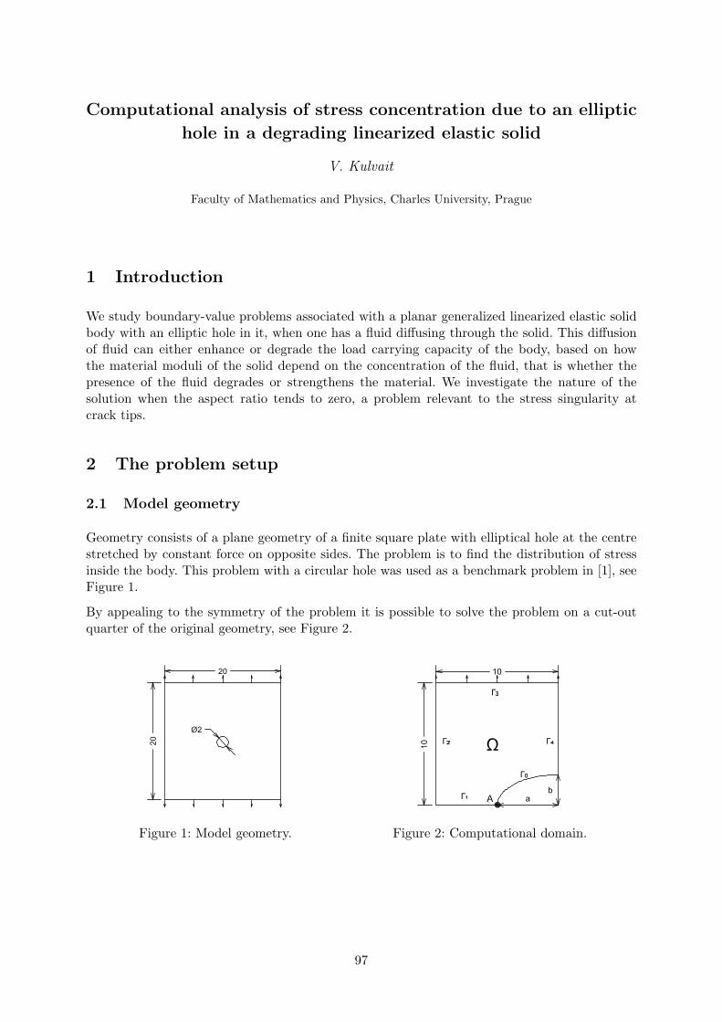
Computational analysis of stress concentration due to an elliptic

hole in a degrading linearized elastic solid

V. Kulvait

Faculty of Mathematics and Physics, Charles University, Prague

1 Introduction

We study boundary-value problems associated with a planar generalized linearized elastic solidbody with an elliptic hole in it, when one has a fluid diffusing through the solid. This diffusionof fluid can either enhance or degrade the load carrying capacity of the body, based on howthe material moduli of the solid depend on the concentration of the fluid, that is whether thepresence of the fluid degrades or strengthens the material. We investigate the nature of thesolution when the aspect ratio tends to zero, a problem relevant to the stress singularity atcrack tips.

2 The problem setup

2.1 Model geometry

Geometry consists of a plane geometry of a finite square plate with elliptical hole at the centrestretched by constant force on opposite sides. The problem is to find the distribution of stressinside the body. This problem with a circular hole was used as a benchmark problem in [1], seeFigure 1.

By appealing to the symmetry of the problem it is possible to solve the problem on a cut-outquarter of the original geometry, see Figure 2.

Figure 1: Model geometry. Figure 2: Computational domain.

97

2.2 Governing equations

For the displacement field u : Ω → R2, corresponding to that of the linearized elastic solid withelastic moduli dependent on the concentration c of the fluid diffusing through the material, thegoverning equations take the form:

0 = grad (λ(c)divu) + div (µ(c)(gradu+ (gradu)T )), (1a)

∂c

∂t= div (kgrad c). (1b)

Thus, the Cauchy stress tensor τ takes the form

τ = λ(c)divuI + µ(c)(gradu+ (gradu)T ) . (2)

2.3 Boundary and initial conditions

The body is loaded in uniform normal stress T = 4.5 along the y axis direction, and this providesthe boundary condition on Γ3, see Figure 2. We prescribe symmetry boundary conditions onthe Γ1 and Γ4. On the remaining parts of boundary Γ0 and Γ2 we prescribe homogeneous Neu-mann condition. Concerning the boundary conditions for c we set c = 1 on Γ0 and homogeneousNeumann condition on the remaining parts of the boundary. The initial conditions at t = 0 arefor simplicity set to be zero, i.e., u(0, ·) = 0 and c(0, ·) = 0 in Ω.

We carried out computational tests with the values for the model parameters taken partiallyfrom the [1] and partially from [3]. For the particular case considered, k does not depend on c.c ∈ [0, 1]. Due to this setting, the Lame coefficients λ and µ are always positive.

3 Solution for the case of a body whose Lame coefficients de-pend on the concentration

We use the system (1) that takes into account the diffusion of the fluid. Particularly the depen-dence of Lame coefficients on the concentration c takes the form:

λ = λ0(1− c2), µ = µ0(1− c

2). (3)

We examine the value of the components of the stress and strain τ22 and ε22 in the vicinity ofthe point A and their asymptotic behavior. We solve the model by FEM with approximately25.000 elements and 100.000 degrees of freedom.

The calculations were carried out for the time interval t ∈ [0, 30]. First, we study the valueof τ22 and ε22 at point A. Then, we examine the distance d, on the line from A to the upper leftcorner of the geometry, from A to point where the stress drops to half of its value in A. For thestrain ε22, this distance is denoted by dE .

From the Figure 3 we can see that for high values of ratio of a : b, the stress is increasing linearly,like in the purely elastic case, with respect to ratio of a : b. But its increase is slower. The speedof growth of τ22 at the point A is increasing with increasing time. The same is true for ε22 at A.

98

Figure 3: Dependence of τ22 and ε22 at the point A on the ratio of the axes of the ellipse a : bin coupled model.

In the case of elastostatics the values (a/b)2d and (a/b)2dE are approximately constant for suffi-ciently large ratios of a : b. Figure 4 depicts the development of the term (a/b)2d for model (1),depending on the value of a : b. For low ratios of the axes of the ellipse the term (a/b)2d isgreater than for the static problem. The asymptotic behavior of the term (a/b)2d is the same asin the case of an elastic model. The behavior of the term (a/b)2dE for the strain is much moresimilar to the case of elastostatics.

Figure 4: Dependence of term (a/b)2d on the ratio of the axes of the ellipse for coefficient ofdiffusion k = 100. On the right is the case with the stress τ22 and on the left case with thestrain ϵ22.

When the semi-major axis of the ellipse is along the direction of loading, we found that whilethe classical elastostatic case, the stress component τ22 and the strain component ε22 changelinearly with the aspect ratio a : b. However, when diffusion is taking place, we found thatthe components of stress and strain vary non-linearly for small values of the ratio of a : b butthe relationship becomes linear for larger values of the ratio of a : b. This result is depicted inFigure 5.

99

Figure 5: Dependence of τ22 and ε22 at the point A on the ratio of the axes of the ellipse incoupled model.

4 Conclusion

The system that governs the degradation of the linearized elastic solid due to the diffusion ofa fluid leads to stresses and strains that differs significantly from that for the purely linearizedelastic model. Numerical results are consistent with the physical expectation that the stress willincrease with decreasing ellipse’s minor axis b. We find that this increase is linear with respectto the aspect ratio.

Presented results will be published as part of the work [2].

Acknowledgement: V. Kulvait had been partially supported by GACR 201/09/0917.

References

[1] Z. Cai, J. Korsawe, and G. Starke. An adaptive least squares mixed finite element methodfor the stress-displacement formulation of linear elasticity. Numerical Methods for PartialDifferential Equations, 21(1):132–148, 2005.

[2] V. Kulvait, J. Malek, and K. R. Rajagopal. Stress concentration due to an elliptic hole ina degrading linearized elastic solid. Submitted for publication in International Journal ofApplied Mechanics and Engineering, 2009.

[3] A. Muliana, K. R. Rajagopal, and S. Shankar. Degradation of an Elastic Composite Cylinderdue to the Diffusion of a Fluid. Journal of Composite Materials, 43(1):1225–1249, 2009.

100

Theoretical analysis of discrete contact

problems with Coulomb friction

T. Ligursky

Charles University in Prague

1 Introduction

Contact problems describe behaviour of loaded deformable bodies in mutual contact. On thecontacting parts one often has to take into account non-penetration as well as frictional condi-tions. The Coulomb law of friction leads to a complicated mathematical problem, in which a lotof issues are still open. In the static case of linear elasticity, existence results have been obtainedfor a small coefficient of friction F (see e.g. [7, 1]). More recently, it has been proven in [8] thatif a solution possesses a certain property, it is unique provided that F is small enough. On theother hand, some examples of nonuniqueness are known for large F ([3, 4]).

In the finite element setting it is known that the discretized problem admits always a solution.There are even results guaranteeing uniqueness of the solution (see e.g. [2]). However, mostof them are of global nature and need the assumption on the magnitude of the coefficientof friction F again. To the author’s knowledge the only result concerning local uniqueness ofsolutions, which admits even large F , has been presented in [5]. Therein, the discrete problem isformulated as a system of non-smooth equations and a suitable version of the implicit functiontheorem is employed to establish the result.

Having been inspired by this approach, our contribution deals with the local behaviour of discretesolutions. It analyses dependence of solutions not only on the coefficient F as in [5] but also onloading. In fact, the role of loading seems to be important, as well (see e.g. a discrete modelwith non-unique solutions in [6]). Besides, qualitative properties of solutions are given.

Throughout the contribution we shall use the following notation: (., .)n stands for the scalarproduct in Rn, ∥.∥n for the corresponding norm, whereas ∥.∥n,∞ denotes the max-norm in Rn:

∥v∥n,∞ = maxi=1,...,n

|vi|, v = (v1, . . . , vn) ∈ Rn.

The symbol ∥.∥n is also used for the matrix norm in Rn×n generated by the vector norm ∥.∥n.

2 Problem formulation

Let us consider a two-dimensional Signorini problem with Coulomb friction in which the coeffi-cient of friction F depends on the spatial variable. A mixed finite element approximation of thismodel leads to the following variational inequality:

Find (u,λν ,λt) ∈ Rn ×Λν ×Λt(F ,−λν) such that

(Au,v)n = (f ,v)n + (λν ,Bνv)p + (λt,Btv)p ∀v ∈ Rn,

(µν − λν ,Bνu)p + (µt − λt,Btu)p ≥ 0 ∀ (µν ,µt) ∈ Λν ×Λt(F ,−λν),

(M)

101

where u represents the displacement vector, λν and λt are the corresponding normal and tan-gential Lagrange multipliers and n, p stand for the numbers of degrees of freedom and of thecontact nodes, respectively. Further, F = (F1, . . . ,Fp) ∈ Rp

+ characterizes the distribution of Fin the contact nodes and the Lagrange-multiplier sets Λν , Λt(.) are defined by

Λν = Rp−,

Λt(F , g) = µt = (µt,1, . . . , µt,p) ∈ Rp | |µt,i| ≤ Figi ∀ i = 1, . . . , p, g = (g1, . . . , gp) ∈ Rp+.

By A ∈ Rn×n we denote the symmetric stiffness matrix satisfying

∃ γ > 0 : (Av,v)n ≥ γ∥v∥2n ∀v ∈ Rn

and by Bν ,Bt ∈ Rp×n the matrices which represent the linear mappings associating with a dis-placement vector its normal and tangential component on the contact zone, respectively. Nextwe suppose that:

(j ) the Euclidean norm of each row vector of Bν , Bt is equal to one;

(jj ) each column of Bν , Bt contains at most one nonzero element;

(jjj ) ∃β > 0 : sup0=v∈Rn

(µν ,Bνv)p + (µt,Btv)p∥v∥n

≥ β∥(µν ,µt)∥2p ∀ (µν ,µt) ∈ R2p.

Finally, f ∈ Rn is the load vector.

3 Theoretical results

In this talk it will be shown that there exists at least one solution to problem (M) for any f ∈ Rn,F ∈ Rp

+ and that this solution is unique provided that ∥F∥p,∞ < βγ/∥A∥n. Furthermore,confining ourselves to F such that ∥F∥p,∞ ≤ Fmax for an arbitrary Fmax ∈ [0, βγ/∥A∥n), theunique solution is a Lipschitz-continuous function of F :

∃ δ > 0 : ∥Sf (F)− Sf (F)∥n+2p ≤ δ∥F − F∥p,∞ ∀F , F ∈ Rp+, ∥F∥p,∞, ∥F∥p,∞ ≤ Fmax.

Here Sf : Rp+ → Rn × Rp × Rp denotes the solution map for a fixed f ∈ Rn:

Sf (F) = (u,λν ,λt), F ∈ Rp+, ∥F∥p,∞ ≤ Fmax,

where (u,λν ,λt) is the solution to (M) with the coefficient F and the load vector f .

To present local analysis of the solutions we shall restrict ourselves to coefficients F from thefollowing set:

A = F ∈ Rp | Fi > 0 ∀ i = 1, . . . , p.

In addition, we shall introduce the Lagrange-multiplier set Λt(.) which does not depend on F :

Λt(g) := µt = (µt,1, . . . , µt,p) ∈ Rp | |µt,i| ≤ gi ∀ i = 1, . . . , p, g = (g1, . . . , gp) ∈ Rp+.

The equivalent formulation of (M) reads as follows:

Find (u,λν ,λt) ∈ Rn ×Λν ×Λt(−λν) such that

(Au,v)n = (f ,v)n + (λν ,Bνv)p + (Fλt,Btv)p ∀v ∈ Rn,

(µν − λν ,Bνu)p + (F (µt − λt),Btu)p ≥ 0 ∀ (µν ,µt) ∈ Λν ×Λt(−λν),

(M∗)

where F := F (F) = diagF1, . . . ,Fp ∈ Rp×p.

102

Our first result concerning local uniqueness of solutions to (M∗) says that the analysis of localbehaviour of a solution as a function of the coefficient F can be converted to the one of localbehaviour of the solution as a function of the load vector f . To state the assertion more preciselywe introduce the set-valued mappings S∗

F : Rn ⇒ Rn+2p and S∗f : A ⇒ Rn+2p by

S∗F (f) = y, f ∈ Rn,

S∗f (F) = y, F ∈ A,

where y, y ≡ (u,λν ,λt), denotes the set of all solutions to problem (M∗) with the coeffi-cient F and the load vector f in both cases. The only difference between these mappings isthat S∗

F associates the set of solutions to varying f for F fixed whereas S∗f associates the set of

solutions to varying F for f fixed.

Theorem 1 Let F0 ∈ A, f ∈ Rn be arbitrary and let y0 ≡ (u0,λ0ν ,λ

0t ) ∈ Rn+2p be a solution

to (M∗) with the coefficient F0 and the load vector f . If S∗F0 has a locally Lipschitz-continuous

branch containing y0 in a vicinity of f ∈ Rn, i.e. there exist a single-valued Lipschitz-continuousfunction φF0 from a neighbourhood O of f into Rn+2p and a neighbourhood V of y0 such that

φF0(f) = y0 and φF0(ξf ) = S∗F0(ξf ) ∩ V ∀ ξf ∈ O,

then there are neighbourhoods U , V of F0, y0, respectively, and a single-valued Lipschitz-continuous function σf : U → V satisfying

σf (F0) = y0 and σf (F) = S∗f (F) ∩ V ∀F ∈ U .

To complete this analysis we shall give sufficient conditions guaranteeing the existence of locallyLipschitz-continuous branches of the solution map S∗

F for F ∈ A fixed. We shall also show thatthese conditions are not satisfied only for f restricted to a union of some subspaces of dimensionstrictly lower than n.

4 An elementary example

In the end of the talk our theoretical approach will be illustrated on an elementary examplecorresponding to a single linear triangular finite element depicted in Figure 1. This example istaken from [5] and it is nothing else than a special case of a model studied in [6].

Denoting u := (uν , ut) and f := (fν , ft), its formulation can be written as follows:

Find (uν , ut, λν , λt) ∈ R4 such that

auν − but − λν − fν = 0,

− buν + aut − λt − ft = 0,

λν − P(−∞,0](λν − ruν) = 0,

λt − P[Fλν ,−Fλν ](λt − rut) = 0,

where the constants a := (λ + 3µ)/2 and b := (λ + µ)/2 depend on the Lame coefficientsλ ≥ 0, µ > 0 characterizing the considered isotropic and homogeneous material and r > 0 is anarbitrarily chosen parameter. Further, P(−∞,0] and P[Fλν ,−Fλν ] are projections of R1 onto theintervals (−∞, 0] and [Fλν ,−Fλν ], respectively.

103

f

zero Dirichletcondition

finiteelement

rigid foundation

Figure 1: Geometry of the elementary example.

It will be shown that the unicity of the solutions to this example depends not only on thecoefficient F but also on the load vector f . Moreover, we shall see that the structure of solutionswith respect to f is much simpler than the one with respect to F .

Acknowledgements: This work has been supported by the grant No. 18008 of the CharlesUniversity Grant Agency and under grant No. 201/07/0294 of the Grant Agency of the CzechRepublic. The support of the Necas Center for Mathematical Modeling is also acknowledged.Last but not least, the author would like to thank Prof. Jaroslav Haslinger for his help andconstructive discussions.

References

[1] C. Eck, J. Jarusek: Existence results for the static contact problem with Coulomb friction.Math. Models Methods Appl. Sci. 8(3), 445-468, 1998.

[2] J. Haslinger: Approximation of the Signorini problem with friction, obeying the Coulomblaw. Math. Methods Appl. Sci. 5, 422–437, 1983.

[3] P. Hild: An example of nonuniqueness for the continuous static unilateral contact modelwith Coulomb friction. C. R., Math., Acad. Sci. Paris 337(10), 685–688, 2003.

[4] P. Hild: Non-unique slipping in the Coulomb friction model in two-dimensional linear elas-ticity. Q. J. Mech. Appl. Math. 57(2), 225–235, 2004.

[5] P. Hild, Y. Renard: Local uniqueness and continuation of solutions for the discrete Coulombfriction problem in elastostatics. Quart. Appl. Math., 63, 553–573, 2005.

[6] V. Janovsky: Catastrophic features of Coulomb friction model. The Mathematics of FiniteElements and Applications IV, MAFELAP 1981, Proc. Conf., Uxbridge/Middlesex 1981,259–264, 1982.

[7] J. Necas, J. Jarusek, J. Haslinger: On the solution of the variational inequality to the Signo-rini problem with small friction. Boll. Unione Mat. Ital., V. Ser., B, 17, 796–811, 1980.

[8] Y. Renard: A uniqueness criterion for the Signorini problem with Coulomb friction. SIAMJ. Math. Anal. 38(2), 452–467, 2006.

104

Fast boundary elements for 3D Helmholtz equation

D. Lukas1, J. Szweda2

1Department of Applied Mathematics2Department of Mechanics, VSB–Technical University of Ostrava

We are faced with a problem of acoustic noise analysis of a railway wheel while aiming at shapeoptimization of its profile such that scattering at certain frequencies will be damped in the end.This contribution presents the related forward problem and its efficient numerical solution usinga novelty variant of the adaptive cross approximation algorithm when applied to hypersingularor double–layer Helmholtz operators, the compression time of which originally suffers from themultiple-element support of the piecewise linear ansatz functions.

1 Galerkin direct BEM for the exterior Helmholtz problem

We consider an elastic structure of a railway wheel fixed along the axle and loaded with a har-monic force on the perimeter. For a given material density ρ, elastic modulus E, Poisson ratio ν,damping β and a load f of an angular frequency ω, we search for the harmonic displacementfield U(x, t) := Reu(x) eiωt such that

−∇ · σ(u)− ρω2 u = 0 in Ω,u = 0 on ΓD,

σ · n = fn δa on ΓN,

where σij(u) = λδij∇ · u + µ(∂iuj + ∂jui), λ := Eν(1+ν)(1−2ν) (1 + 2βi), µ := E

2(1+ν) (1 + 2βi),and δa is a boundary Dirac distribution at a ∈ ΓN. For the numerical solution we employ thelowest–order tetrahedral finite elements.

The resulting deformations provide the Neumann boundary data for the exterior Helmholtzproblem

−p− κ2 p = 0, in Ωe := R3 \ Ω,∂p/∂n = vn := ω2ρu · n, on Γ := ∂Ω,∣∣∣( x

|x| ,∇p(x))− iκp(x)

∣∣∣ = O(|x|−2), x → ∞,

where κ := ω/c with the speed of sound c. The acoustical pressure is given by P(x, t) :=Rep(x) eiωt. We consider the Galerkin direct approach to the boundary integral equation ofthe latter problem, cf. [1], which reads as follows: Find p ∈ H−1/2(Γ) such that

∀v ∈ H−1/2(Γ) : ⟨Dp, v⟩Γ = ⟨(−1/2I +K ′)vn, v⟩Γ,

where I denotes the identity, the Helmholtz fundamental solution reads P (x,y) := eiκr/(4π|r|)with r := |x− y| and where

⟨Dp, v⟩Γ :=∫Γ

∫Γ

P (x,y)[(n(x)×∇v(x)) · (n(y)×∇p(y))−κ2n(x)v(x) · n(y)p(y)

]dS(y) dS(x),

⟨K ′vn, v⟩Γ :=

∫Γ

∫Γ

(∂P (x,y)/∂n(y)) vn(y)v(x) dS(y) dS(x).

We employ the lowest–order boundary element discretization using a numerical quadrature ofregularized kernels [2].

105

2 Element–based adaptive cross approximation

Typically, the boundary of the railway wheel is discretized into 15112 triangles and 22668 no-des, therefore, we aim at a sparsification of the orginally fully populated BEM matrices. Theadaptive cross approximation (ACA) [3] turns out to be a good choice. It relies on a hierar-chical decomposition of a matrix into the admissible (far field) and nonadmissible (near field)blocks so that the nonadmissible blocks are assembled completely, while the admissible ones areadaptively approximated by a sum of rank–one matrices. The algorithm is easy to include intoan existing code, since it only requires assembling of rows and columns. This works fast for thelowest–order discretization of the single–layer V as well as the double–layer operator K, sinceeither the rows or columns are related to the piecewise constant ansatz functions. However, incase of the hypersingular matrix D the piecewise linear ansatz functions have multi–elementsupports, thus, the entry evaluation costs more, moreover, the quadrature over many couplesof elements is performed several times. In our case, the ACA applied to K compressed to 12%takes 25 minutes, while it takes 3.4 hours in the case of D compressed to 15%. Note that this isnot the case for the Laplace problem, since we have the representations D = T T

· V · T.

As a remedy for the Helmholtz operator D, we propose to hierarchically cluster the matrixelement–wise, rather than nodal–wise, and approximate the admissible blocks by piecewise con-stant ansatz functions, instead of piecewise linear, while using the admissible part of V similarlyto the Laplace case. Our element–based ACA approximation is as follows:

D =∑i

∑j

D(i,j) =∑i

∑j

T Ti Vij Tj − κ2RT

i

∫Γi

∫Γj

P (x,y)ϕ(i)k (x)ϕ

(j)l (y) dS(y) dS(x)

k,l

Rj

≈ T T · V adm · T − κ2

4

∑(i,j)∈N adm

RTi ·(1/2 1/2

)· V adm

ij ·(1/21/2

)·Rj +

∑(i,j)∈Nnon

D(i,j),

where N adm and N non denotes the admissible and the nonadmissible blocks, respectively. Here,each element couple is entered at most once. In our case, the matrix D was assembled in lessthan one hour. However, the application of D costs more. Note that our approach can also beapplied to K.

Finally, to validate our method, we applied it to a unit ball and cube for the problem with thegiven solution p(x) := eiκ|x−xs|/(4π|x − xs|), where κ := 2π 151.6/340 and with the scattererplaced at xs := (0.05, 0.05, 0.05). For example, the ball surface was discretized on 6 levels into40–40960 elements. the relative solution error measured in L2(Γ) converged from 10−1 to 10−4.The ACA assembling time for D at the finest level took 42397 seconds comparing 5515 secondsin our approach, however, the 123 GMRES iterations took 496 seconds vers. our 6662 seconds.

References

[1] O. Steinbach, S. Rjasanow: The Fast Solution of Boundary Integral Equations. Springer,2007.

[2] S. Sauter, C. Schwab: Randelementmethoden: Analyse, Numerik und Implementierungschneller Algorithmen. B.G. Teubner, Stuttgart, Leipzig, Wiesbaden, 2004.

[3] M. Bebendorf, R. Grzhibovskis: Accelerating Galerkin BEM for linear elasticity using adap-tive cross approximation. Math. Meth. Appl. Sci. 29, 1721–1747, 2006.

106

A recursive formulation of limited memory

variable metric methods

L. Luksan, J. Vlcek

Institute of Computer Science, Academy of Sciences of the Czech RepublicPod Vodarenskou vezı 2, 182 07 Praha 8, and

Technical University of Liberec, Halkova 6, 461 17 Liberec

Variable metric methods with limited memory can be efficiently used for large-scale uncon-strained optimization in case the sparsity pattern of the Hessian matrix is not known. Thesemethods are usually realized in the line-search framework so that they generate a sequence ofpoints xi ∈ Rn, i ∈ N , by the simple process

xi+1 = xi + αidi, (1)

where di = −Higi is a direction vector, Hi is a positive definite approximation of the inverseHessian matrix and αi > 0 is a scalar step-size chosen in such a way that

Fi+1 − Fi ≤ ε1 αi dTi gi, dTi gi+1 ≥ ε2 d

Ti gi (2)

(the weak Wolfe conditions), where Fi = F (xi), gi = ∇F (xi) and 0 < ε1 < 1/2, ε1 < ε2 < 1.Matrices Hi, i ∈ N , are computed either by using a limited number (m≪ n) of variable metricupdates applied to the scaled unit matrix or by updating low dimension matrices. The firstapproach, used in [9], is based on the computation of the direction vector di using the Strangrecurrences [8]. The second approach, used in [1], is based on the matrix expression describedbelow. To simplifying notation, we omit index i and replace index i+ 1 by +.

Variable metric method from the Broyden class use the update

H+ = H + UMUT = H + [d,Hy]

[m1, m2

m2, m3

] [dHy

]= H +

1

bddT − 1

aHy(Hy)T +

η

a

(abd−Hy

)(abd−Hy

)T, (3)

where d = x+−x, y = g+−g, a = yTHy, b = yTd and η is a free parameter. We need to expressm consecutive steps of (3) (with the initial matrix γI) in the form H+ = γI + UMUT , whereU ∈ Rn×2m and M ∈ R2m×2m. In [1], the authors propose explicit expressions of the matrixM for three classic variable metric updates: DFP (η = 0), BFGS (η = 1) and the rank one(η = b/(b − a)). For other values of the parameter η, such explicit expressions are not known.In this contribution we describe another way, based on recursive construction of the matrix M ,which allows us to realize any member of the Broyden class of the variable metric updates. Thefollowing theorem is proved in [7].

Theorem 1 Let H+ be a matrix defined by (3) and H = γI + UMUT . Then

H+ = H1 + U+M+UT+ ,

where U+ = [U , d, H1y] and

M+ =

M +m3 zzT , m2 z, m3 z

m2 zT , m1, m2

m3 zT , m2, m3

. (4)

Here m1 = (1/b)(ηa/b + 1), m2 = −η/b, m3 = (η − 1)/a are elements of matrix M , z = M rand r = UT y.

107

If i ≤ m, the construction of matrix Hi+1 follows straightforwardly from Theorem 1. Thuswe describe the construction of matrix Hi+1 in case i > m. We will assume that Hi+1−m =γiI. At the beginning of the i-th iteration, we have available the rectangular matrix Ui−1 =[di−m, yi−m, . . . , di−1, yi−1] and the block upper triangular matrix

Ri−1 =

dTi−myi−m, . . . dTi−myi−1

yTi−myi−m, . . . yTi−myi−1

. . . . . . . . . . . . . . . . . . . . .0, . . . dTi−1yi−1

0, . . . yTi−1yi−1

,whose every block contains two rows and one column. First we determine matrixUi = [di−m+1, yi−m+1, . . . , di, yi] from matrix Ui−1 by deleting the first two columns and addingthe last two columns. Similarly easily we obtain matrix Ri from matrix Ri−1. Only the lastcolumn UT

i yi of this matrix has to be computed. Furthermore, we compute recursively matrixMi = M i

i in such a way that we set

M ii−m+1 =

[m1

i−m+1, m2i−m+1

m2i−m+1, m3

i−m+1

]

(indices 1, 2, 3 are now placed up) and for i−m+1 ≤ j ≤ i−1, compute vector zj = M ij rj , where

rj is j − i +m-th column of matrix Ri, whose every even element is multiplied by number γi(since Hi+1−m = γiI), and set

M ij+1 =

M ij +m3

j+1 zjzTj , m2

j+1 zj , m3j+1 zj

m2j+1 z

Tj , m1

j+1, m2j+1

m3j+1 z

Tj , m2

j+1, m3j+1

.Vector Hi+1gi+1 is computed by the formula

Hi+1gi+1 = γigi+1 + [di−m+1, γiyi−m+1, . . . , di, γiyi] Mi

[di−m+1, γiyi−m+1, . . . , di, γiyi]T gi+1

(even columns of matrix Ui are multiplied by number γi). As we can see, approximately6mn operations (addition and multiplication) are consumed in i-th iteration. However, approxi-mately 2(m − 1)n operations can be saved, if we compute and store inner products dTj gi+1,

yTj gi+1 instead of dTj yi, yTj yi, i−m+1 ≤ j ≤ i. Then the first m− 1 inner products dTj yi, y

Tj yi,

i −m + 1 ≤ j ≤ i − 1 can be determined from the previously computed inner products by theformulas dTj yi = dTj gi+1−dTj gi, yTj yi = yTj gi+1− yTj gi, i−m+1 ≤ j ≤ i− 1. Thus it is necessary

to compute only two inner products dTi yi, yTi yi. Inner products d

Tj gi+1, y

Tj gi+1, i−m+1 ≤ j ≤ i

can be used for the computation of direction vector si+1, so we save 2mn operations.

The method described has been tested by using a set of 60 test problems with 1000 variables.This set (Test25) was obtained by merging the sets Test14, Test15, Test18 described in [6], whichcan be downloaded from http://www.cs.cas.cz/luksan/test.html (together with report [6]).The results of the tests are listed in Table 1, where NIT is the total number of iterations, NFVis the total number of function and gradient evaluations, NF is the number of failures and TIME

is the total CPU time. We have tested the original LBFGS subroutine, described in [2], and ourrealizations of limited memory variable metric methods implemented in the UFO system [5]. InTable 1, BFGSSTR denotes the limited memory BFGS method with the Strang recurrences [9] (ananalogy of LBFGS), BFGSBNS denotes the limited memory BFGS method with compact matricesdescribed in [1], BFGSNEW denotes the limited memory BFGS method with recursive construction

108

of matrix M described above, LMVMNEW denotes the limited memory variable metric method withrecursive construction of matrix M that use parameter η proposed in [4], and CG denotes theconjugate gradient method. Note that the first four rows in Table 1 correspond to differentimplementations of the BFGS method and that our approach gives the best results.

Method NIT NFV F TIME

LBFGS 110406 117226 2 43.38BFGSSTR 99125 104085 - 37.56BFGSBNS 91650 96235 - 36.89BFGSNEW 85430 89796 - 33.50LMVMNEW 92877 99033 - 34.61

CG 144990 222460 1 60.77

Table 1: Test results.

Acknowledgement: This work has been supported by the Czech science foundation, projectNo. 201/09/1957, and the institutional research plan No. AV0Z10300504.

References

[1] R.H.Byrd, J.Nocedal, R.B.Schnabel: Representation of quasi-Newton matrices and their usein limited memory methods. Math. Programming 63, 129-156, 1994.

[2] D.C.Liu, J.Nocedal: On the limited memory BFGS method for large scale optimization.Mathematical Programming 45, 503-528, 1989.

[3] L.Luksan: Numericke optimalizacnı metody. Nepodmınena minimalizace. Vyzkumna zpravaV-1058, Ustav informatiky AV CR, Praha 2009.

[4] L.Luksan, E.Spedicato: Variable metric methods for unconstrained optimization and nonli-near least squares. Journal of Computational and Applied Mathematics 124, 61-93, 2000.

[5] L.Luksan, M.Tuma, J.Vlcek, N.Ramesova, M.Siska, J.Hartman, C.Matonoha: InteractiveSystem for Universal Functional Optimization. Research Report V-1040, Institute of Com-puter Science Czech Academy of Sciences, Prague 2008.

[6] L.Luksan, J.Vlcek: Sparse and partially separable test problems for unconstrained and equa-lity constrained optimization. Research Report V-767, Institute of Computer Science, CzechAcademy of Sciences, Prague 1998.

[7] L.Luksan, J.Vlcek: Limited memory variable metric methods from the Broyden class. Re-search Report V-1059, Institute of Computer Science Czech Academy of Sciences, Prague2009.

[8] H.Matthies, G.Strang: The solution of nonlinear finite element equations. Int. J. for Nume-rical Methods in Engineering 14, 1613-1623, 1979.

[9] J. Nocedal: Updating quasi-Newton matrices with limited storage. Math. Comp. 35, 773-782,1980.

109

Quantitative analysis of numerical solution

for the Gray-Scott model

J. Mach

Czech Technical University, Prague

1 Introduction

Reaction-diffusion systems are a class of systems of partial differential equations of parabolictype. It includes mathematical models describing various phenomena e.g. in the fields of physics,biology and chemistry. Gray-Scott model is one of these models. It was first introduced in 1984by P. Gray and S. K. Scott [1]. It is a mathematical model of the autocatalytic chemical reactionU +2V −−→ 3V , V −−→ P . U , V are reactants and P is final product of the reaction. Chemicalsubstance U is being continuously added into the reactor and the product P is being continuouslyremoved from the reactor during the reaction. Later it has been extensively studied e.g. byWei [2], Winter [3], Ueyama [5], Dkhil [6], Doelman [7]. This model is well known to exhibit richdynamics, see e.g. Nishiura [4]. There exist chemical systems exhibiting features similar to thoseof the Gray-Scott model, see e.g. Mazin [8] and references therein.

2 Problem formulation

We study the Gray-Scott in 2D. Assume that Ω ≡ (0, L)× (0, L) is an open square representingthe square reactor, where the chemical reaction takes place, ∂Ω is its boundary andν is its outernormal. Then initial-boundary value problem for the Gray-Scott model is a system of two partialdifferential equations of parabolic type ut = a∆u− uv2 + F (1− u), vt = b∆v + uv2 − (F + k)vin Ω×(0, T ) with initial conditions u(·, 0) = uini, v(·, 0) = vini and zero Neumann boundaryconditions ∂u

∂ν |∂Ω= 0, ∂v∂ν |∂Ω= 0. Functions u, v are unknowns representing concentrations of

chemical substances U , V . Parameter F denotes the rate at which the chemical substance Uis being added during the chemical reaction, F + k is the rate of V → P transformation anda, b are constants characterizing the environment in the reactor. This system may be rewrittenin several dimensionless forms. We use the one which is used also e.g. in [3, 8, 9].

3 Numerical schemes

Computational studies of the Gray-Scott model show difficulties in convergence. We comparetwo numerical schemes for solution of the initial-boundary value problem defined in Sect. 2 inorder to disclose details of these problems. Both of them are based on the method of lines.For spatial discretization we used structured numerical grids consisting of squares for the finitedifference method and of triangles for the finite elements method To solve resulting systems ofordinary differential equations Runge-Kutta-Merson method (see e.g. [10], [11]) was used.

110

3.1 FDM based numerical scheme

Let h be mesh size such that h = L/(N − 1) for some N ∈ N+. We define numerical gridas set ωh = (ih, jh) | i = 0, . . . , N − 1, j = 0, . . . , N − 1. For function u : R2 → R we definea projection on ωh as uij = u (ih, jh). We introduce finite differences ux1,ij = (ui+1,j − ui,j)/h,ux1,ij = (ui,j − ui−1,j)/h ux2,ij = (ui,j+1 − ui,j)/h, ux2,ij = (ui,j − ui,j−1)/h, and define approxi-mation ∆h of the Laplace operator ∆ as ∆huij = ux1x1,ij + ux2x2,ij . Then semi-discrete schemehas the following form

d

dtuij(t) = a∆huij + F (1− uij)− uijv

2ij ,

d

dtvij(t) = b∆hvij − (F + k)vij + uijv

2ij , (1)

plus discrete initial and boundary conditions. This system is solved by Runge-Kutta-Mersonmethod.

3.2 FEM based numerical scheme

To induce the semi-discrete scheme we begin with variational formulation of the problem definedin Sect. 2 and rewrite it in weak form. Then we proceed to discretize this problem in space. LetTh be a partition of domain Ω into disjoint triangles τ . At vertices Pj of Th we define pyramidfunctions Φ1, . . . ,ΦNh

, Φi(Pj) = δij and define finite dimensional space Sh ⊂ H1(Ω) to bespanned by these functions. We search for Galerkin approximation uh, vh of weak solution in Shthus uh =

∑Nh1 αjΦj and vh =

∑Nh1 βjΦj . Real-valued functions αj , βj are solution of Galerkin

approximation problem

d

dt(uh, φ1) + a(∇uh,∇φ) = (f1, φ), ∀φ ∈ Sh

d

dt(vh, φ2) + b(∇vh,∇φ) = (f2, φ), ∀φ ∈ Sh

with uh|t=0= uini,h, vh|t=0= vini,h, where f1(u, v) = F (1−u)−uv2, f2(u, v) = −(F+k)v+uv2 and(·, ·) denote the L2 inner product. Substituting basis functions Φ1, . . . ,ΦNh

instead of arbitraryfunctions φ ∈ Sh we get system of 2Nh ODEs with initial conditions

A ˙α(t) + aBα(t) = C(α(t), β(t)),

A ˙β(t) + bBβ(t) = E(α(t), β(t)),

Aα(0) = D,

Aβ(0) = F. (2)

Lagrange interpolation was used for numerical integration to get approximation of vectors C, E,D, F . Using method of lumped masses and renumbering unknowns we can rewrite the problemfor finding functions αj , βj in the following form

d

dtuij(t) =

2a

3h2[ui+1,j + ui+1,j+1 + ui,j−1 + ui,j+1 + ui−1,j +

+ui−1,j+1 − 6uij ] + F (1− uij)− uijv2ij

d

dtvij(t) =

2b

3h2[vi+1,j + vi+1,j+1 + vi,j−1 + vi,j+1 + vi−1,j +

+vi−1,j+1 − 6vij ]− (F + k)vij + uijv2ij (3)

plus corresponding initial and boundary conditions. This system is solved by Runge-Kutta-Merson method.

111

4 Numerical simulations

We performed a series of computations to perform quantitative comparison of our 2D numericalschemes. According to our results the Gray-Scott model is sensitive on the mesh parameter size,which means, the numerical solution may change notably when refining the computational grid.

In our numerical simulations we use square domain Ω ≡ (0.0, 0.5)×(0.0, 0.5). Initial data areconsidered such that uini + vini = 1 hold within the computational domain Ω and vini consistsof one or several spots.

We met initial data and model parameter values combinations for which the following situationsoccurred. First, we have results where FDM based numerical scheme is less dependent on thespace stepping, that is, the numerical results are visually more similar in wider range of meshparameter sizes then in case of the FEM based numerical scheme. We have also results, wherethe FEM based numerical scheme is less dependent on the space stepping. We were able to seeagreement in numerical results obtained in both of these cases from certain mesh parametersize. But we have also met combinations where we were not able to see the solutions becomingvisually more and more similar while refining the numerical grid. Example is given below inFig. 1.

(a), FDM, grid 800×800 (b), FEM, grid 800×924

Figure 1: Dependence of pattern in numerical solution on numerical scheme and grid size forgiven model parameters (a = 2 · 10−5, b = 1 · 10−5, F = 0.0737, k = 0.061882, L = 0.5) andinitial data (one spot in the middle of the domain) at fixed time t=8000.

In Fig. 1 we demonstrate the case, where we were not able to obtain agreement of numericalresults by the numerical schemes from Sect. 3. Using the same model parameters and initial datawe could see lines growing in orthogonal directions. Depicted are solutions at time t = 8000.Each of numerical schemes provided the same pattern within wide range of grid sizes. We triedto successively refine the numerical grid up to 2000×2000 and corresponding size of triangle grid.For the same model parameters as in Fig. 1 an agreement of numerical results was observed fordifferent initial data.

112

5 Conclusion

We focused on quantitative comparison of two numerical schemes which solve the Gray-Scottmodel in 2D. Our numerical simulations show that for certain combinations of initial data andmodel parameter values we may not get an agreement of numerical results provided by thesenumerical schemes while refining the numerical grid. Example result is given.

Acknowledgement: The work has been performed under the Project HPC-EUROPA(RII3-CT-2003-506079), with the support of the European Community - Research InfrastructureAction under the FP6 “Structuring the European Research Area” Programme. Partial supportof the project of “Necas Center for Mathematical modeling”, No. LC06052 and of the project“Applied Mathematics in Physics and Technical Sciences”, No. MSN6840770010 of the Ministryof Education, Youth and Sports of the Czech Republic is acknowledged.

References

[1] P. Gray, S.K. Scott: Autocatalytic reactions in the isothermal, continuous stirred tank reac-tor: oscillations and instabilities in the system A+2B → 3B, B → C. In: Chem. Eng. Sci.,39, 1087–1097, 1984.

[2] J. Wei: Pattern formation in two-dimensional Gray-Scott model: existence of single-spotsolutions and their stability. In: Physica D, 148, 20–48, 2001.

[3] J. Wei, M. Winter: Asymmetric spotty patterns for the Gray-Scott model in R2. In: Stud.Appl. Math., 110(1), 63–102, 2003.

[4] Y. Nishiura, D. Ueyama: Self-Replication, Self-Destruction, and Spation-Temporal Chaos inthe Gray-Scott model. In: Forma, 15, 281–289, 2000.

[5] Y. Nishiura, D.Ueyama: Spatio-temporal chaos for the Gray-Scott model. In: Physica D, 150,137–162, 2001.

[6] F. Dkhil, E. Logak, Y. Nishiura: Some analytical results on the Gray-Scott model. In:Asymptotic Analysis, 39, IOS Press, 225–261, 2004.

[7] A. Doelman et al.: Pattern formation in the one-dimensional Gray-Scott model. In: Nonli-nearity, 10, 523–563, 1997.

[8] W. Mazin, K.E. Rasmussen, E. Mosekilde et al.: Pattern formation in the bistable Gray-Scott model. In: Mathematics na Computers in Simulations, 40, Elsevier Science, 371–396,1996.

[9] J.S. McGough, K. Riley: Pattern Formation in the Gray-Scott model. In: Nonlinear Analysis:Real World Application, 5, Elsevier Science, 105–121, 2004.

[10] J. Sembera, M. Benes: Nonlinear Galerkin Method for Reaction-Diffusion Systems Admit-ting Invariant Regions. In: Journal of Computational and Applied Mathematics, 136(1-2),163–176.

[11] V. Minarik, J. Kratochvıl, K. Mikula, M. Benes: Numerical simulation of dislocation dy-namics. In: Numerical Mathematics and Advanced Applications, ENUMATH 2003 (peerreviewed proceedings), Springer Verlag, 631–641, 2004.

113

Effect of hydrodynamic mixing on the photosynthetic

microorganism growth: Revisited

S. Papacek, C. Matonoha

Institute of Physical Biology, University of South Bohemia, Nove Hrady

Institute of Computer Science, Academy of Sciences of the Czech Republic, Prague

1 Introduction

Biotechnology with microalgae and photo-bioreactor (PBR) design is nowadays regaining atten-tion thanks to emerging projects of CO2 sequestration and algae biofuels. Nevertheless, there donot exist reliable methods as well as programming software neither for modeling, simulation andcontrol of microbial growth in photo-bioreactors, nor for PBR design [3]. Modeling in a predictiveway the photosynthetic response in the three-dimensional flow field seems today unrealistic, be-cause the global response depends on numerous interacting intracellular reactions, with varioustime-scales. The physiological state of any cellular system and its impact on growth and productformation is the result of a complex interplay between the extracellular environment and thecellular machinery. The design of PBR in which microalgae cells function as factories as wellas the prediction of suitable PBR operating conditions is further complicated because of thedynamic variations of the extracellular environment.

Our main goal is to develop and implement the mathematical model of microalgae growth ina general PBR as tool in the design of photo-bioreactors and the optimization of their per-formance. In our previous works we studied an adequate multi-scale lumped parameter modelwhich well describes the principal physiological mechanisms in microalgae: photosynthetic light-dark reactions and photoinhibition [5], as well as its model parameter estimation [8, 7]. In [6] wepresented how to construct a distributed parameter model consisting mainly in determinationof hydrodynamic dispersion coefficient as function of space coordinates.

This paper deals with the non-homogeneous steady-state one-dimensional reaction-diffusion sys-tem (3) with a special boundary condition. However, equation (3) is rewritten in form of twoordinary differential equations (ODE), which leads after re-scaling to the standard form of thesingularly perturbed system [4]. The purpose of such an operation is to infer the asymptoticproperties of the reaction-diffusion system (3).

2 Modelling photosynthetic microorganism growth

The photosynthetic microorganism growth description is usually based on the so-called microbialkinetics, i.e. on the lumped parameter models (LPM) describing the photosynthetic responsein small cultivation systems with a homogeneous light distribution [9]. However, there is animportant phenomenon, the so-called flashing light enhancement, which demands some othermodel than it residing in the artificial connection between the steady state kinetic model andthe empiric one describing the photosynthetic productivity under fluctuating light condition.Nevertheless, even having an adequate dynamical LPM of microorganism growth, see e.g. phe-nomenological model of so-called photosynthetic factory [5, 8], another serious difficulty residesin the description of the microalgal growth in a PBR, i.e. in a distributed parameter system.

114

In order to develop the distributed parameter model (DPM) of a microorganism growth, twomain approaches for transport and bioreaction processes modelling are usually chosen:(i) Eulerian infinitesimal, and (ii) Eulerian multicompartmental. While the Eulerian infinitesimalapproach, leading to the partial differential equations (PDE), is an usual way to describe trans-port and reaction systems, the multicompartmental modelling framework, resulting in an ODEsystem, is mostly used in the process engineering area. This second approach, based on balanceequation among compartments with finite control volume, has been recently treated by Bezzo etal. [2]. The authors presented there a rigorous mathematical framework for constructing hybridmulticompartment/CFD models. Hybrid there means that the fluid flow description is resolvedby a CFD code, and does not make a part of the ODE system of governing equations.

In the sequel, we adopt the first approach aiming to clarify in an analytical manner the role ofhydrodynamic mixing, or more precisely, the mechanism of the photosynthetic microorganismgrowth enhancement due to the microbial cell transport by radial dispersion. Nevertheless, in thefuture work, our results should serve to develop a numerical scheme for setting up the optimalcompartment size in the multicompartment/CFD models.

3 Model development

Transport equation for microbial cells (concentration c) as the function of spatial coordinatesand time gets the next form [1]:

∂c

∂t+∇ · (vc)−∇ · (De∇c) = R(c) , (1)

where R(c) is the source term (representing microbial growth, unit: cell m−3s−1), v representsthe velocity field, and De is the dispersion coefficient, which corresponds to diffusion coefficientin microstructure description and becomes mere empirical parameter suitably describing mixingin the system. De is influenced by the molecular diffusion and velocity profile. When mixing ismainly caused by the turbulent micro-eddies, the phenomenon is called the turbulent diffusionand a turbulent diffusion coefficient is introduced e.g. in [1]. The reaction obviously dependson some variables, usually called as substrates. For our special case of photosynthetic growthin a PBR, the role of only one limiting substrate (the nutrients are supposed to be present ina sufficient amount, i.e. they do not limit the growth) fulfills the irradiance, in other words,an external forcing input u. Moreover we suppose the rectangular PBR geometry illuminatedfrom one side, i.e. the irradiance level is decreasing from the PBR wall to PBR core. Thus, thePBR volume (our computational domain) can be divided into layers with the same irradiancelevel, transforming the 3D problem into the one-dimensional. Consequently, the description ofcell motion in direction of light gradient, i.e. perpendicular to PBR wall and at the same timeperpendicular to the direction of convective flow, is of most interest. This motion is caused bythe just mentioned turbulent diffusion. Furthermore, we can introduce the dimensionless spatialcoordinate x, and the dimensionless dispersion coefficient p(x) by

r := xL , De := p(x) D0 ,

where L and D0 (unit: m2s−1) are the PBR length in direction of light gradient, and a constantwith some characteristic value, respectively.

Furthermore we introduce the dimensionless concentrations c and css as

y :=c

cm, yss :=

csscm

,

where cm is a characteristic (e.g. maximal) concentration of c.

115

Based on the photosynthetic factory model [5, 8] we have for the reaction term R the relation

R(c) = −k (c− css) , (2)

where k is the rate (unit: s−1) associated with the dynamic process by which is the concentration capproaching to some value css depending only on the external input u(x).

As we are interested on the steady state solution of (1), i.e. ∂c∂t = 0, we finally obtain

−[p(x)y′

]′+ q(x) y = q(x) yss, y′(0) = 0, y′(1) = 0 , (3)

where q(x) := k(u(x)) L2

D0.

4 Asymptotic properties of the reaction-diffusion system (3)

In the process engineering literature, there exists a concept of well mixed unit. This constructis further used e.g. in the multicompartmental or multizonal models [2, 6]. The crucial questionis: When a compartment with finite volume is well mixed? For a reaction-diffusion system, ithas to depend on the so-called Damkohler number.

In our previous work, in sake of the benchmark problem, we were looking for an analytical so-lution of the equation (3). Realizing that it was impossible, we did not search the solution inthe usual form of y = y(x), but we wanted to find the mean value of y in the interval x ∈ [0.1],i.e. to compute the expression

∫ 10 y(x) dx. Based on [10], the boundary value problem (3) was

transformed into the related initial value problem. It consisted in finding solutions of two homo-geneous equations, two differential equations with the right-hand side and computing a solutionof a system of two algebraic equations. By this procedure, we could have obtained a functionvalue and its derivative in an arbitrary point. The original differential equation with boundaryconditions was thus transformed into a differential equation with an initial condition. As wehave needed only a solution in several points, we could apply the above procedure repeatedly.Finally, the value

∫ 10 y(x) dx would be obtained by a suitable numerical method.

Now, we are developing an asymptotic method. Let first define ddxy := z, then the resulting first

order ODE system is

d

dxy = z ,

d

dx[p(x)z] = q(x) (y − yss) , z(0) = 0, z(1) = 0 . (4)

Consequently, if we define k0 as follows: k := kA(u(x)) k0, then the Damkohler number of

second type could be defined as DaII := k0L2

D0, and the dependence of the solution of (4) on

DaII := ε→ 0 could be studied.

The following ODE (5)

d

dx[p(x)z] = εkA(u(x)) (y − yss) , z(0) = 0, z(1) = 0 , (5)

thanks to the properties of its right hand side clearly satisfies the sufficient condition for applyingthe averaging method [4]. One can therefore approximate (4) as follows (always when ε→ 0):

d

dxy = z ,

d

dx[p(x)z] = ε

∫ 1

0[kA(u(x)) (y − yss)] dx , z(0) = 0, z(1) = 0 . (6)

116

Acknowledgement: This work was supported by the grant MSMT MSM 600 766 58 08 of theMinistry of Education, Youth and Sports of the Czech Republic, and by the Grant Agency ofCzech Republic through the research grant No. 102/05/0011.

References

[1] W.J. Beek, K.M.K. Muttzall, J.W. van Heuven: Transport Phenomena. Wiley & Sons, 2000.

[2] F. Bezzo, S. Macchietto, C.C. Pantelides: Computational issues in hybrid multizo-nal/computational fluid dynamics models. AIChE Journal, 51, 1169–1177, 2005.

[3] M. Janssen, J. Tramper, L.R. Mur, R.H. Wijffels: Enclosed Outdoor Photobioreactors: Li-ght Regime, Photosynthetic Efficiency, Scale-Up, and Future Prospects. Biotechnology andBioengineering, 81, 193–210, 2003.

[4] H.K. Khalil: Perturbation and averaging. Nonlinear systems. Prentice Hall, 2002.

[5] S. Papacek, S. Celikovsky, D. Stys, J. Ruiz-Leon: Bilinear system as modelling frameworkfor analysis of microalgal growth. Kybernetika, 43, 1–20, 2007.

[6] S. Papacek, D. Stys, P. Dolınek, K. Petera: Multicompartment/CFD modelling of trans-port and reaction processes in Couette-Taylor photobioreactor. Applied and ComputationalMechanics, 1, 577–586, 2007.

[7] S. Papacek, S. Celikovsky, B. Rehak, D. Stys: Experimental design for parameter estimationof two time-scale model of photosynthesis and photoinhibition in microalgae. Math. Comput.Simul., doi: 10.1016/j.matcom.2009.06.033, 2009.

[8] B. Rehak, S. Celikovsky, S. Papacek: Model for Photosynthesis and Photoinhibition: Para-meter Identification Based on the Harmonic Irradiation O2 Response Measurement. IEEETransactions on Circuits and Systems I: Regular Papers, Special Issue: 101–108.

[9] K. Schugerl, K.-H. Bellgardt: Bioreaction Engineering, Modeling and Control. Springer-Verlag, Berlin Heidelberg, 2000.

[10] E. Vitasek: Numericke metody, Nakladatelstvı technicke literatury, Praha, 1987.

117

Modelling of the airflow through vocal folds

J. Prokopova, M. Feistauer, V. Kucera, J. Horacek

Charles University, Faculty of Mathematics and Physics, Prague

Institute of Thermomechanics, Academy of Sciences of the Czech Republic, Prague

1 Introduction

The simulation of compressible flow in time dependent domains plays an important role in severalareas of human activities, for example development of aircrafts and turbines, civil engineering, carindustry or medicine. The presented work introduces implementation of numerical techniqueslike the ALE (Arbitrary Lagrangian-Eulerian) methods and the discontinous Galerkin finiteelement methods in these domains and creates the bases of the further work in the direction offluid-structure interaction. We are specially interested in the medical apllications of this type ofproblem. For this reason the problem of the airflow through vocal folds is treated.

2 Continuous problem

We deal with compressible flow in a bounded domain Ωt ⊂ IR2 depending on time t ∈ [0, T ].We assume that the boundary of Ωt consists of three disjoint parts ∂Ωt = ΓI ∪ΓO ∪ΓWt , whereΓI and ΓO represent the inlet and outlet and ΓWt represents moving impermeable walls.

We consider the Navier-Stokes equations in the conservative form [1]:

∂w

∂t+

2∑s=1

∂fs(w)

∂xs=

2∑s=1

∂Rs (w,∇w)

∂xsin Ωt, t ∈ [0, T ] , (1)

where

w = (ρ, ρv1, ρv2, E)T ∈ IR4,

fs(w) = (ρvs, ρv1vs + δ1sp, ρv2vs + δ2sp, (E + p)vs)T , s = 1, 2,

Rs (w,∇w) = (0, τs1, τs2, τs1v1 + τs2v2 + k∂θ

∂xs)T , s = 1, 2,

τij = λδijdivv + 2µdij(w), dij(w) =1

2

(∂vi∂xj

+∂vj∂xi

), i, j = 1, 2.

We use the following notation: ρ – density, p – pressure, E – total energy, (v1, v2) – velocityvector, θ – absolute temperature, cv > 0 – specific heat at constant volume, γ > 1 – Poissonadiabatic constant, µ > 0, λ – viscosity coefficients, k > 0 – heat conduction coefficient. We setλ = −2µ/3. System (1) is completed by the thermodynamical relations

p = (γ − 1)(E − ρ |v|2 /2), θ =

(E

ρ− 1

2|v|2

)/cv, (2)

118

and equipped with inicial condition w(x, 0) = w0(x), x ∈ Ωt and boundary conditions:

Inlet ΓI : ρ|ΓI×(0,T ) = ρD,

v|ΓI×(0,T ) = vD = (vD1, vD2)T ,

2∑j=1

(2∑

i=1

τijni

)vj + k

∂θ

∂n= 0 on ΓI × (0, T );

Moving wall ΓW : vΓW×(0,T ) = zD,∂θ

∂n= 0;

Outlet ΓO :

2∑i=1

τijni = 0,∂θ

∂n= 0 j = 1, 2.

Here zD is the velocity of the moving wall.

3 ALE formulation

The time dependence of the domain is taken into account with the aid of a regular one-to-oneALE mapping (cf. [3])

At : Ω0 −→ Ωt, i.e. At :X 7−→ x = x(X, t) = At(X). (3)

We define the ALE velocity:

z(X, t) =∂

∂tAt(X), t ∈ [0, T ], X ∈ Ω0, (4)

z(x, t) = z(A−1t (x), t), t ∈ [0, T ], x ∈ Ωt

and the ALE derivative of a function f = f(x, t) defined for x ∈ Ωt and t ∈ [0, T ]:

DA

Dtf(x, t) =

∂f

∂t(X, t), where f(X, t) = f(At(X), t), X ∈ Ω0. (5)

By the chain rule,DAf

Dt=∂f

∂t+ z · ∇f =

∂f

∂t+ div (zf)− f div z. (6)

This leads us to the ALE form of the Navier-Stokes equations:

DAw

Dt+

2∑s=1

∂gs(w)

∂xs+wdivz =

2∑s=1

∂Rs (w,∇w)

∂xs, (7)

where gs(w) = fs(w)− zsw, s = 1, 2.

4 Discretization

The problem is discretized in space by the discontinuous Galerkin finite element method ([1], [2])using piecewise polynomial approximations of the components of the state vector w, in generaldiscontinuous on interfaces between neighbouring elements from a triangulation of the polygonalapproximation Ωht of the domain Ωt. In this work we use the simplest variant of the discontinuous

119

Galerkin finite element method for solving Navier-Stokes equations, the incomplete interiorpenalty Galerkin (IIPG) scheme.

Scheme obtained by space discretization by the discontinuous Galerkin finite element methodrepresents a system of ordinary differential equations, which must be discretized with respect totime. We use the method developed in [2] for inviscid flow. A backward Euler method is usedfor a discretization of the ALE derivative

DAwh

Dt(x, tk+1) ≈

wk+1h (x)− wk

h(x)

τk, x ∈ Ωhtk+1

, (8)

where wjh(x) = wj

h

(Atj

(A−1

tk+1

)(x)), x ∈ Ωhtk+1

and wjh(x) = wh(x, tj). The nonlinear

terms in the scheme are linearized with the aid of properties of expressions gs and Rs. Thistreatment leads to the linear system,which is is solved on each time level by the GMRES methodwith a block diagonal preconditioning.

5 Numerical experiments

We consider compressible flow in the channel, whose shape is inspired by a shape of vocal foldsand supraglottal spaces as shown in Figure 1. The lower channel wall between the points Aand D is changing the shape according to the given function of time and axial coordinate:

y(x, t) = (a1 + at)

[sin

(3π

2+ π

x− xAxC − xA

)+ 1

]+ d, x ∈ [xA, xC ], (9)

y(x, t) = 2(a1 + at)cos

(π

2

x− xCxD − xC

)+ d, x ∈ [xC , xD],

at = a2sin (2πft) , t ∈ [0, T ]; a1 = 0.18, a2 = 0.015,

where f = 5.38 · 103. The motion of the upper wall of the channel is treated in a similar way.This movement is interpolated inside the domain resulting in the ALE mapping At.

Figures 2 show streamlines at different time instants t = 504, 558, 612, 666 during the fourthperiod of the motion.

6 Conclusion

Using our program code based on the finite element approximation, we solved the viscous com-pressible flow in time-dependent domains with shape motivated by the simulation of the airflow

Figure 1: Geometry of computational domain.

120

Figure 2: Streamlines at time t = 504, 558, 612, 666.

in human vocal folds. The computational results show that it is not possible to simplify themathematical model supposing the axisymmetry of the solution, because the unsymmetric flowstructure is developed in spite the computational domain is axisymmetric.

Future work will be focused on the better approximation of the computational domain to the realgeometry of the glottis and the vocal tract and mainly on the application of the fluid-structureinteraction consisting in the solution of coupled system describing flow and structure behaviour.

Acknowledgement: This work was supported by the Project OC 09019 ”Modelling of voiceproduction based on biomechanics”within the program COST 2103 and by the project No. MSM0021620839 of the Ministry of Education of the Czech Republic.

References

[1] M. Feistauer, J. Felcman, J. Straskraba:Mathematical and Computational Methods for Com-pressible Flow. Clarendon Press, Oxford, 2003.

[2] M. Feistauer, V. Kucera, J. Prokopova: Discontinuous Galerkin solution of compressibleflow in time dependent domains.. In: Mathematics and Computers in Simulation. In press,doi: 10.1016/j.matcom.2009.01.020.

[3] T. Nomura, T.J.R. Hughes: An arbitrary Lagrangian-Eulerian finite element method forinteraction of fluid and a rigid body. Comput. Methods Appl. Mech. Engrg. 95, 115–138,1992.

121

Algebraic multilevel preconditioning of coarse problems

of balanced domain decomposition methods

with nodal constraints

I. Pultarova

Department of Mathematics, Faculty of Civil Engineering, CTU in Prague

1 Coarse problems of balanced domain decomposition methodsby constraints

A method of balanced domain decomposition by constraints (BDDC) [3] is an iterative algori-thm for numerical solution of partial differential equations discretized by the finite element (FE)method. The BDDC method exploits a nonoverlaping partition of a domain, and within eachiteration, the main computation consists in solving particular boundary problems on every sub-domain and in solving a certain coarse grid problem. There are many ways how to define thecoarse base functions. In our considerations, they are defined by nodal values (degrees of freedom,DOFs) in few nodes on interfaces of subdomains and have minimal energy on each subdomainand null normal derivatives on all interfaces. Then in general, the coarse functions are discon-tinuous on interfaces of subdomains up to the nodes where the coarse DOFs are defined. Sincethe coarse problem itself can be large, an appropriate preconditioning is desired [2].

2 Algebraic multilevel preconditioning of the coarse problem

We present a new strategy of preconditioning of the coarse problem of BDDC. This is based onan algebraic multilevel (AML) preconditioning technique [1]. In spite of classical application ofAML preconditioning directly to finite element bases, we utilize a hierarchical splitting of thecoarse space within the BDDC algorithm. A quality of AML preconditioning is measured by theconstant γ in the strengthened Cauchy-Buniakowski-Schwarz (CBS) inequality [1].

We provide some numerical estimates of the CBS constants for two- and three-dimensionalelliptic problems: an equation of diffusion and an equation of linear elasticity. For discretisation,bilinear or trilinear FEs are used with rectangular or prismatic supports, respectively. Thesubdomains are of a rectangular or prismatic shape as well. Coarse base functions are definedby all corner nodal values on subdomains. In every problem a hierarchical splitting of the coarsebase system is constructed with coefficients that are equal to that for hierarchical transformationof bilinear or trilinear FEs, respectively. In each test we specify only a bilinear form a(·, ·) usedin a weak formulation of the problem, because neither boundary conditions nor a right handside of the equation influence the estimates of the CBS constant γ. The estimate of γ can becalculated from exploiting the properties of the coarse function on a single reference subdomainonly. A mesh of a reference subdomain may influence the value of γ. Then in each graph,a number of elements in a reference subdomain is indicated. Our main interest is to examinea behavior of γ when varying the coefficients of the bilinear form a(·, ·).

122

Diffusion equations (D2) and (D3). Bilinear form a(·, ·) is

a(u, v) =

∫Ω(∇u)TC∇v dx,

where

C =

(1 cc d

)or C =

1 c12 c13c12 d2 c23c13 c23 d3

for two- and three-dimensional problems (D2) and (D3), respectively. The values of c, d, diand cij are constant on subdomains and matrix C is positive definite on every subdomain.

The estimates of γ2 for the case c = 0 and d ∈ (0, 1⟩ are displayed in Figure 1 on the left for fivedifferent meshes of a reference subdomain. On the right, values of γ2 are presented for d = 1 andc ∈ (−1, 0⟩. The estimates of γ2 for the case d2 = 1, cij = 0 and d3 ∈ (0, 1⟩ are shown in the leftpart of Figure 2 for four different meshes of a reference prismatic subdomain. In the right handside of Figure 2, values of γ2 for the case di = 1 and c12 = c13 = c23 ∈ (−0.5, 0⟩ are presented.

0 0.2 0.4 0.6 0.8 10.3

0.35

0.4

0.45

0.5

0.55

0.6

0.65

0.7

0.75

c = 0, d Î (0,1]

γ2

1 x 12 x 250 x 501 x 502 x 50

−1 −0.8 −0.6 −0.4 −0.2 00.3

0.35

0.4

0.45

0.5

0.55

0.6

0.65

0.7

0.75

d = 1, c Î (−1,0]

γ2

1 x 12 x 250 x 501 x 502 x 50

Figure 1: Numerical estimates of γ2 for hierarchical splitting of coarse problems forequation (D2). Coefficients c = 0 and d ∈ (0, 1⟩ (left), and the case d = 1 and c ∈ (−1, 0⟩(right).

0 0.2 0.4 0.6 0.8 10.5

0.6

0.7

0.8

0.9

1

cij = 0, d

2 = 1, d

3 Î (0,1]

γ2

1 x 1 x 12 x 2 x 212 x 12 x 121 x 1 x 12

−0.5 −0.4 −0.3 −0.2 −0.1 00.5

0.6

0.7

0.8

0.9

1

di = 1, c

12 = c

13 = c

23 Î (−0.5,0]

γ2

1 x 1 x 12 x 2 x 212 x 12 x 121 x 1 x 12

Figure 2: Numerical estimates of γ2 for hierarchical splitting of coarse problems of BDDC forequation (D3). Coefficient d2 = 1 and cij = 0 and varying d3 ∈ (0, 1⟩ (left), and d2 = d3 = 1and c12 = c13 = c23 ∈ (−0.5, 0⟩ (right) for different meshes of a reference subdomain.

123

Elasticity equations (E2) and (E3). Bilinear form a(·, ·) is

a(u,v) =

∫Ω2µ(∇(s)u)T∇(s)v + λ divu · divv dx,

where ∇(s)u = ε(u) and

εij(u) =1

2

(∂ui∂xj

+∂uj∂xi

).

The share modulus of a material µ and the Lame constant λ can be substituted by the Poissonratio ν and by the modulus of elasticity E via µ = E/2/(1 + ν) and λ = Eν/(1 + ν)/(1− 2ν).

The estimates of γ2 for elasticity equations for ν ∈ ⟨0, 0.5) can be found in Figure 3. Two-dimensional cases for partitions of a rectangular subdomain 1× 1, 5× 5, 50× 50 and 1 × 50,respectively, are shown on the left. A three-dimensional case for five different meshes of a refe-rence prismatic subdomain can be found in the right part of Figure 3.

0 0.1 0.2 0.3 0.4 0.50.4

0.45

0.5

0.55

0.6

0.65

0.7

0.75

0.8

0.85

0.9

ν Î [0,0.5)

γ2

1 x 15 x 550 x 501 x 50

0 0.1 0.2 0.3 0.4 0.50.65

0.7

0.75

0.8

0.85

0.9

0.95

1

ν Î [0,0.5)

γ2

1 x 1 x 12 x 2 x 212 x 12 x 121 x 1 x 122 x 2 x 12

Figure 3: Numerical estimates of γ2 for hierarchical splitting of the coarse problems for equati-ons (E2) (left) and (E3) (right). Varying Poisson ratio ν ∈ ⟨0, 0.5) and different meshes ofa reference subdomains.

Acknowledgement: The research was supported by the project CEZ MSM 6840770001 andby the Grant Agency of The Czech Republic, No. 201/09/P500.

References

[1] O. Axelsson: Iterative Solution Methods. Cambridge University Press, 1996.

[2] J. Mandel, B. Sousedik, C.R. Dohrmann: Multispace and Multilevel BDDC. Computing 83,55-85, 2008.

[3] Numerical Methods in Computational Mechanics, 2009, Edited by M. Okrouhlık. e-book,http://www.it.cas.cz/files/u1784/Num methods in CM.pdf.

124

Hybrid dynamical systems: verification

and error trajectory search

S. Ratschan

Institute of Computer Science

Academy of Sciences of the Czech Republic

Modern complex technical systems usually consist not only of physical components, but alsoof computer equipment interacting with these physical components. As a consequence, suchsystems cannot be modeled based on physical laws formulated in the language of continuousmathematics alone. In addition, one needs discrete modeling formalisms. Hybrid (dynamical)systems are a formalism for modeling the resulting combined continuous-discrete behavior. Inthe talk we will describe this formalism, and discuss algorithms for the automatic analysis ofsuch hybrid systems.

When restricted to their continuous part, such hybrid systems amount to ordinary differentialequations, when restricted to their discrete part, to finite state machines. However, the inter-action between those two parts introduces significant additional difficulty that obstructs the useof classical numerical error analysis. Moreover, such systems are usually non-deterministic, inthe sense that they not only have a single initial state, but a whole set of initial stats, and in thesense that starting from a given unique state, they may allow an uncountable set of trajectories(e.g., resulting from differential inequalities). A further difficulty results from the fact that oneis often interested in analyzing the behavior of hybrid systems over an unbounded time horizon.

As a consequence, more or less all problems of analyzing hybrid systems are undecidable [4],although one can get much further with a weaker notion of quasi-decidability [3, 1, 5].

In the talk we will discuss discuss algorithms for proving that a given hybrid system does notreach an element of a set of states considered to be unsafe (in whatever unbounded time) [6, 2].Moreover, we will discuss the use of optimization techniques to find trajectories the violate thisproperty [7].

Acknowledgement: This work has been supported by GACR grant 201/08/J020 and by theinstitutional research plan AV0Z100300504.

References

[1] W. Damm, G. Pinto, and S. Ratschan. Guaranteed termination in the verification of LTLproperties of non-linear robust discrete time hybrid systems. International Journal of Foun-dations of Computer Science (IJFCS), 18(1):63–86, 2007.

[2] T. Dzetkulic and S. Ratschan. How to capture hybrid systems evolution into slices of parallelhyperplanes. In ADHS’09: 3rd IFAC Conference on Analysis and Design of Hybrid Systems,pages 274–279, 2009.

[3] M. Franzle. Analysis of hybrid systems: An ounce of realism can save an infinity of states.In J. Flum and M. Rodriguez-Artalejo, editors, Computer Science Logic (CSL’99), number1683 in LNCS. Springer, 1999.

125

[4] T. A. Henzinger, P. W. Kopke, A. Puri, and P. Varaiya. What’s decidable about hybridautomata. Journal of Computer and System Sciences, 57:94–124, 1998.

[5] S. Ratschan. Safety verification of non-linear hybrid systems is quasi-decidable. 2009. sub-mitted.

[6] S. Ratschan and Z. She. Safety verification of hybrid systems by constraint propagationbased abstraction refinement. ACM Transactions in Embedded Computing Systems, 6(1),2007.

[7] S. Ratschan and J.-G. Smaus. Finding errors of hybrid systems by optimising an abstraction-based quality estimate. In C. Dubois, editor, Tests and Proofs, volume 5668 of LNCS, pages153–168. Springer, 2009.

126

Comparison of the sparse matrix storage formats

I. Simecek

Faculty of Information Technologies,

Czech Technical University, Prague

1 Introduction

Computations with sparse matrices are widespread in scientific projects. The performance ofmathematical operations with sparse matrices depends strongly on the used matrix storageformat. In this paper, we compare the performance during the execution of some basic routinesfrom linear solvers and its dependency on the used format.

The paper consists of four parts: a general introduction of sparse matrix storage formats, per-formance testing, conclusions, and suggestions for future work.

2 Usual sparse matrix formats

In the following text, we assume that A is real sparse matrix of order n. Let nZ be the totalnumber of nonzero elements in A.

2.1 The coordinate (XY) format

The coordinate (XY) format is the most simplest sparse format. The matrix A is represented bythree linear arrays Elem,X, and Y . The array Elem[1, . . . , nZ] stores the nonzero values of A,arrays X[1, . . . , nZ] and Y [1, . . . , nZ] contain X- and Y -positions, respectively, of the elementswith the nonzero value.

2.2 The compressed sparse row (CSR) format

The most common format (see [4]) for storing sparse matrices is the compressed sparse row (CSR)format. A matrix A stored in the CSR format is represented by three linear arrays Elem,Addr,and Ci. The array Elem[1, . . . , nZ] stores the nonzero elements of A, the array Addr[1, . . . , n]contains indexes of initial nonzero elements of rows of A, and the array Ci[1, . . . , nZ] containscolumn indexes of nonzero elements of A. Hence, the first nonzero element of row j is stored atthe index Addr[j] in array Elem.

2.3 Register blocking formats

Widely-used formats(XY and CSR) are easy to understand, however sparse operations (likematrix-vector or matrix-matrix multiplication) using these formats are slow (mainly due to in-direct addressing). Sparse matrices often contain dense submatrices (blocks), so various blockingformats were designed to accelerate matrix operations. Compared to the CSR format, the aim of

127

these formats (like SPARSITY[2] or CARB[3]) is to consume less memory and to allow a betteruse of registers and the vectorization of the computation. Algorithms using these formats arevery fast, because they are tuned for a target architecture.

2.4 Quadtree data format

Quadtree (for details see [6, 5, 1]) is the recursive tree data structure. Such a tree representsa partition of the matrix into submatrices (“nodes” in the graph terminology). There are differenttypes of nodes in the tree. Inner nodes of the quadtree are divided into “Mixed” or “Empty”nodes. Leafs of the quadtree are divided into “Full” or “Empty” nodes.

Great advantages of the quadtree are the following:

• Easy and fast conversion from common sparse matrix storage formats like CSR or XY.

• Modifications (adding or removing nonzero elements) of the quadtree are relatively easy.

• The recursive style of programming and recursive style of storage (“Divide and Conquer”approach) leads to codes with a surprising performance due to the better cache memoryutilization.

3 Discussion about formats

3.1 Drawbacks of usual formats

• XY and CSR formats: These formats doesn’t support fast adding or removing nonzeroelements.

• Register blocking formats: These formats suffer from a large transformation overhead,are designed only for limited set of operations, doesn’t support fast adding or removingnonzero elements.

• Quadtree data format: A big drawback of the quadtree structure is a larger controland data overhead compared to standard formats. The standard quadtree implementationleads to a space (and execution) inefficiency. To remove inefficiencies, we use the additionaltypes of leafs: modified versions of the XY and the CSR formats. The modification meansthat we express all coordinates relatively to the beginning of the submatrix (node). Wecall “XY” and “CSR” respectively this type of node.

Our second improvement is the elimination of “Empty” nodes, because they do not containany useful information. They are simply represented by the NULL pointer.

3.2 Dynamic formats

All mentioned formats (except quadtree) doesn’t support fast adding or removing nonzero ele-ments. We must modify previous formats to eliminate this drawback. For example, the imple-mentation of the CSR format is modified in this way: The array Addr[1, . . . , n] contains pointersto rows of A (separated arrays containing the values of nonzero elements and its column indexes).Since all information are stored in dynamic arrays, we called these modified formats “dynamic”.

128

3.2.1 Combined format

The new “combined” format consists of dynamic CSR and CSC format. So, this format consumestwo times more space but it should be fast independently on the memory pattern (row-like orcolumn-like).

4 Evaluation of the results

4.1 Test applications

We have implemented these basic routines from the linear algebra that are often used in linearsolvers:

• to get an value at the given location in the sparse matrix (operation GET XY),

• to set an value at the given location in the sparse matrix (operation SET XY),

• to find the maximal value in the row in the sparse matrix (operation MAX),

• to add values of given row to other row in the sparse matrix (operation ADD),

• the transposition of the sparse matrix (operation TRANSP),

• the multiplication of a sparse matrix by a dense vector (operation SPMV),

4.2 Test data

We have used 32 real matrices from various technical areas from the MatrixMarket and Harwellsparse matrix test collection.

4.3 HW and SW configuration

All results were measured on Intel Core 2 Quad Q8200 (only one core was used) at 2.33 GHz,4 GB of the main memory at 400 MHz, running OS Windows XP Professional SP3 with thefollowing cache parameters: L1 cache is 32 KB data cache, L2 cache is 2 MB data.SW: Microsoft Visual Studio 2003, Intel compiler version 10.1 with switches for maximal per-formance.

4.4 Measured results

Comments on Table 1:

• The performance of GET XY and SET XY operations depend on the ratio nZn , for higher

values (“long” rows) can be improved by the binary search method.

• The performance of SET XY operation is different in the case if the former value of givenlocation is nonzero (the update of the value=hit) or is zero (the new nonzero entry=miss).

• The TRANSP operation in Combined format consists only of exchanging few pointers!

129

operation/format CSR CSC Combined Quad

operation GET XY 0 . . .++ 0 . . .++ 0 . . .++ +operation SET XY (hit) 0 . . .++ 0 . . .++ 0 . . .++ +operation SET XY (miss) − . . .+ − . . .+ − . . . 0 +

operation MAX ++ − ++ +operation ADD ++ −− − 0

operation TRANSP 0 0 ++ +operation SPMV + − + 0

Table 1: Performance comparison of the formats. The symbol −− denotes very slow, − denotesslow, 0 denotes average, + denotes fast, ++ denotes very fast.

5 Conclusion

We have tested the performance of some very basic routines used in linear solvers. Measuredresults satisfy the theoretical assumption that used data format affects strongly the performance.Since every format has some drawbacks and overheads, it is difficult to choose a “winner”, but ifthe numbers of these operations and the memory pattern are known, we can choose the suitabledata storage format.

6 Future works

• We should optimize some routines and deeply measure the performance on various plat-forms.

• We should develop a new format similar to combined format but with “weak coherency”.

Acknowledgement: This research has been supported by MSMT under research programMSM6840770014.

References

[1] J.D. Frens, D.S. Wise: Matrix inversion using quadtrees implemented in gofer. 1995.

[2] E. Im: Optimizing the Performance of Sparse Matrix-Vector Multiplication - dissertationthesis. Dissertation thesis, University of Carolina at Berkeley, 2001.

[3] I. Simecek: A new format for sparse matrix-vector multiplication. In: Seminar on NumericalAnalysis, Ostrava, Ustav geonomy AV CR, 101–104, 2007.

[4] I. Simecek: Performance aspects of sparse matrix-vector multiplication. Acta Polytechnica,46(3/2006), 3–8, January 2007.

[5] D.S. Wise: Matrix algorithms using quadtrees (invited talk). In: ATABLE-92, 11–26, 1992.

[6] D.S. Wise: Ahnentafel indexing into morton-ordered arrays, or matrix locality for free. In:Euro-Par 2000 Parallel Processing, volume 1900 of Lecture Notes in Computer Science,774—783, 2000.

130

Application of the BDDC method to the Stokes problem

J. Sıstek, P. Burda, J. Mandel, J. Novotny, B. Sousedık

Institute of Mathematics, Academy of Sciences of the Czech Republic, PragueDepartment of Mathematics, Faculty of Mechanical Engineering,

Czech Technical University in PragueDepartment of Mathematical and Statistical Sciences,

University of Colorado Denver, Denver, USADepartment of Mathematics, Faculty of Civil Engineering,

Czech Technical University in Prague

1 Introduction

The Balancing Domain Decomposition based on Constraints (BDDC) is one of the most advancedpreconditioners suitable for parallel iterative solution of large systems of linear equations arisingfrom finite element (FE) analysis. The method was introduced by Dohrmann [2] and the theoryis due to Mandel and Dohrmann [6]. Li and Widlund reformulated the BDDC method in [5] toa simple global approach. The underlying theory of the BDDC method covers problems withsymmetric positive definite matrix. An important application that leads to such kind of systemsis structural analysis by linear elasticity theory.

The solution of the incompressible Stokes problem by a mixed finite element method leads toa saddle point system with symmetric indefinite matrix. Thus, the standard theory of BDDCdoes not cover this important class of problems. In the first attempt to apply BDDC to the incom-pressible Stokes problem proposed by Li and Widlund [4], the optimal preconditioning propertiesof BDDC were recovered. The approach is based on the notion of benign subspaces, which isrestricted to using discontinuous pressure approximations, and the authors present results forpiecewise constant approximations. Moreover, the approach in [4] requires quite nonstandardconstraints between subdomains, thus making the implementation more problem specific anddifficult.

In this paper, we follow a different approach. We have implemented a parallel version of theBDDCmethod and verified its performance on a number of problems arising from linear elasticity(e.g. [9]). Here, we investigate the applicability of the method and its implementation to theStokes flow ‘as is’. Although it is beyond the standard theory of the BDDC method, contributiveresults are obtained using only minor changes and minimal amount of custom coding to theimplementation for elasticity problems.

It has been known for a long time, that conjugate gradient method is able to reach solutionalso for many indefinite cases (e.g. [7]), although it may fail in general. Our investigation is alsomotivated by recent trends of numerical linear algebra to investigate and often prefer the use ofPCG method with a suitable indefinite preconditioner over more robust but also more expensiveiterative methods for solving saddle point systems such as MINRES, BiCG or GMRES [8].

Results for the Stokes flow in two and three dimensions are presented. All these problemsare obtained using mixed discretization by Taylor–Hood finite elements. These elements usepiecewise (bi/tri)linear pressure approximation, which does not allow the approach via benignspaces of [4], but are very popular in the computational fluid dynamics community.

131

2 BDDC domain decomposition method

Let Ω be a bounded domain in R2 or R3, let U be a finite element space of piecewise polynomialfunctions v continuous on Ω and U ′ its dual space. Let a(·, ·) be a bilinear form on U × U andf ∈ U ′, and let ⟨·, ·⟩ denote the duality pairing of U ′ and U . Consider an abstract variationalproblem: Find u ∈ U such that

a(u, v) = ⟨f, v⟩ ∀ v ∈ U . (1)

For the case of steady Stokes flow we adopt the following slightly unusual notation

a(u, v) = ν

∫Ω∇uh : ∇vhdΩ−

∫Ωph∇ · vhdΩ +

∫Ωψh∇ · uhdΩ, (2)

⟨f, v⟩ =

∫Ωf · vhdΩ. (3)

Solution u = (uh, ph) consists of the discretized vector field of velocity and the discretized scalarfield of pressure, ν represents the kinematic viscosity of the fluid, f represents the external load,and v = (vh, ψh). For the case of Stokes problem, a(u, v) is only symmetric indefinite [3].

Write the matrix problem corresponding to (1) as Au = f . The domain Ω is decomposedinto N nonoverlapping subdomains Ωi, i = 1, ..., N . Each subdomain is a union of several finiteelements of the underlying mesh. Unknowns common to at least two subdomains are calledboundary unknowns and the union of all boundary unknowns is called the interface Γ. Let Wi

be the space of finite element functions on subdomain Ωi and put W = W1 × · · · ×WN . It isthe space where subdomains are completely disconnected, and functions on them independentof each other. Clearly, U ⊂W .

The main idea of the BDDC preconditioner in the abstract form is to construct an auxiliaryfinite dimensional space W such that

U ⊂ W ⊂W, (4)

and extend the bilinear form a (·, ·) to a form a (·, ·) defined on W × W , such that solving thevariational problem (1) with a (·, ·) in place of a (·, ·) is cheaper and can be split into independentcomputations performed in parallel. Then the solution projected to U is used for the preconditi-oning of (1). Space W contains functions continuous at selected coarse degrees of freedom suchas values at selected nodes called corners as well as averages over edges or faces.

In computation, the corresponding matrix denoted A is used. It is larger than the original matrixof the problem A, but it possesses a simpler structure suitable for direct solution methods. Thisis the reason why it can be used as a preconditioner.

The projection E : W → U is realized as a weighted average of values from different subdomainsat unknowns on the interface Γ followed by the discrete harmonic extension from boundary tointerior of each subdomain (see [9]).

Let r ∈ U ′ be the residual in an iteration of an iterative method. The BDDC preconditionerMBDDC : U ′ → U in the abstract form produces the preconditioned residual v ∈ U as

MBDDC : r → v = Ew,

where w ∈ W is obtained as the solution to problem

w ∈ W : a (w, z) = (r,Ez) ∀z ∈ W , (5)

or in terms of matrices asv = EA−1ET r. (6)

132

no BDDC ILUT with thresholdmethod preconditioner corners only corners+faces 10−3 10−4 10−5

BICGSTAB n/a 45 22 n/a 331 10GMRES 759 49 38 472 87 18

Table 1: Number of iterations for BICGSTAB and GMRES without preconditioning, and pre-conditioned by BDDC and ILU, lid driven cavity.

3 Numerical results

Our parallel implementation of the BDDC preconditioner has been extensively tested on pro-blems with symmetric positive definite matrices arising from linear elasticity (e.g. [9]). Thecurrent version is based on the multifrontal massively parallel sparse direct solver MUMPS [1],which is used for factorization of matrix A in (6). The preconditioned problem is solved byparallel PCG method run on problem (1) reduced to interface Γ by static condensation (see [9]for details). For the Stokes problem, matrix A is symmetric indefinite and as such is factorizedand the problem repeatedly solved by MUMPS representing an indefinite preconditioner.

As the first example, we select a 2D case of lid driven cavity, a popular benchmark problem formethods for viscous flow. The case of uniform mesh of 128 ×128 Taylor–Hood finite elementswas chosen. It was divided into 8 subdomains by METIS package. Solution of the problemby our earlier solver based on a serial frontal algorithm took 231 seconds on one 1.5 GHzIntel Itanium 2 processor of SGI Altix 4700 computer in CTU Supercomputing Centre, Prague,compared to 40.5 seconds on 8 processors of the same computer necessary for the solution by thenew implementation of BDDC. The stopping criterion of PCG was chosen as ∥r∥2/∥g∥2 < 10−6,resulting in 50 PCG iterations. To investigate the performance of the BDDC preconditionerin combination with standard iterative methods for general matrices, namely BICGSTAB andGMRES, we have also performed several experiments with our serial code written in Matlab.In Table 1, we compare the resulting number of iterations of these methods preconditioned byBDDC and by the ILU preconditioner for several values of threshold τ for dropping entries inincomplete factorization. Where ‘n/a’ is present in the table, BICGSTAB failed to converge.

In the second example, a 3D geometry of a channel with a sudden reduction of diameter isconsidered. Due to the symmetry of the channel, only a quarter of it is considered in the compu-tation. This problem consists of 3 393 Taylor–Hood finite elements with 54 248 unknowns, and itis solved to relative residual ∥r∥2/∥f∥2 < 10−6 by 33 PCG iterations. Division into 4 subdomainsobtained by METIS and solution at Reynolds number 100 are presented in Figure 1.

4 Conclusion

We present a parallel implementation of the BDDC preconditioner and explore its applicabilityto problems with indefinite matrices, namely the Stokes problem. Although the available theoryeither does not cover this case, or treats it differently [4], the presented experiments suggestpromising ways for this effort. We have performed several experiments, for which PCG wassuccessfully used although the system was indefinite. However the reason why a breakdown wasnot observed deserves further investigation. Our serial experiments also led to promising resultsfor combination of BDDC method with standard iterative methods for solving systems withgeneral matrices, such as BICGSTAB and GMRES.

133

Figure 1: Division of mesh into 4 subdomains (left) and pressure with streamlines (right) forchannel with sudden reduction of diameter, only a quarter of the channel is considered forsymmetries.

Acknowledgement: This research has been supported by National Science Foundation undergrant DMS-0713876, by Czech Science Foundation under grant GA CR 106/08/0403, and by theGrant Agency of the Academy of Sciences of the Czech Republic under grant IAA200600801.A part of this work was done during Jakub Sıstek’s visit at the University of Colorado Denver.

References

[1] P.R. Amestoy, I.S. Duff, J.-Y. L’Excellent: Multifrontal parallel distributed symmetric andunsymmetric solvers. Comput. Methods Appl. Mech. Engrg. 184 501–520, 2000.

[2] C.R. Dohrmann: A preconditioner for substructuring based on constrained energy minimi-zation. SIAM J. Sci. Comput. 25(1), 246–258, 2003.

[3] H.C. Elman, D.J. Silvester, A.J. Wathen: Finite elements and fast iterative solvers: withapplications in incompressible fluid dynamics. Numerical Mathematics and Scientific Com-putation, Oxford University Press, New York, 2005.

[4] J. Li, O. Widlund: BDDC algorithms for incompressible Stokes equations. SIAM J. Numer.Anal. 44(6), 2432–2455, 2006.

[5] J. Li, O.B. Widlund: FETI-DP, BDDC, and block Cholesky methods. Internat. J. Numer.Methods Engrg. 66(2), 250–271, 2006.

[6] J. Mandel, C.R. Dohrmann: Convergence of a balancing domain decomposition by constraintsand energy minimization. Numer. Linear Algebra Appl. 10(7) 639–659, 2003.

[7] C.C. Paige, M.A. Saunders: Solutions of sparse indefinite systems of linear equations. SIAMJ. Numer. Anal. 12(4), 617–629, 1975.

[8] M. Rozloznık, V. Simoncini: Krylov subspace methods for saddle point problems with indefi-nite preconditioning. SIAM J. Matrix Anal. Appl. 24(2), 368–391, 2002.

[9] J. Sıstek, J. Novotny, J. Mandel, M. Certıkova, Burda, P.: BDDC by a frontal solver andstress computation in a hip joint replacement. Mathematics and Computers in Simulation,in print, available online January 21, 2009, DOI 10.1016/j.matcom.2009.01.002 (2009).

134

Modelovanı podzemnıho proudenı jako sdruzene ulohy

v 3D-2D-1D geometrii se slozitou diskretizacı

I. Skarydova, M. Hokr

Technicka univerzita v Liberci

1 Uvod

V prıspevku se zabyvame modelovanım rezimu proudenı vody v okolı vodarenskeho tuneluv Bedrichove v Jizerskych horach, v podobe sdruzene ulohy podzemnıho a povrchoveho proudenı.Pritom vyuzıvame modelu s 3D-2D-1D geometriı a vypocet provadıme v programu Flow123D [1],vyvıjenem na Technicke univerzite v Liberci. Uloha je narocna na diskretizaci kvuli specifickemutvaru modelu (lokality), ktery je charakterizovan velkym pomerem mezi vertikalnımi a hori-zontalnımi rozmery a prıtomnostı tunelu s velmi malym prumerem proti rozmerum ulohy.

Ulohu resıme v ramci projektu Decovalex, ktery se zabyva simulacı termo-hydro-mechano-chemickych (THMC) procesu za ucelem analyzy hlubinneho uloziste a bezpecneho ukladanıjaderneho odpadu. Spojitost zde nalezame v podobnem charakteru lokality z hlediska prırodnıchpodmınek, s obdobnymi tunely v horninovem masivu se pocıta i v hlubinnem ulozisti.

2 Popis modelu

Uloha je definovana jako potencialove proudenı (parabolicke parcialnı diferencialnı rovnice 2.ra-du) v oblasti, ktera je kombinacı oblastı ruznych dimenzı Ω = Ω1 ∪ Ω2 ∪ Ω3 (tzv.

”multidimen-

zionalnı model“, podrobneji v [2]), vyjadrene jako system Darcyho zakona a rovnice kontinuity

ui = −Ki∇pi na Ωi , i = 1, 2, 3 (1)

κi∂pi∂t

−∇ · ui = qi na Ωi , i = 1, 2, 3 (2)

kde ui [m.s−1] je tzv. darcyovska rychlost (odpovıda plosne hustote toku), Ki [m.s−1] hydrau-licka vodivost a pi [m] piezometricka vyska, κ [m−1] specificka storativita, qi [s

−1] zdroje t [s]cas [3]. Na castech hranice oblasti predepisujeme standardnı Dirichletovy a Neumannovy okra-jove podmınky. Uloha je numericky resena pomocı smısene-hybridnı metody konecnych prvku,ktera umoznuje prirozene zavedenı interakce mezi jednotlivymi dimenzemi v diskretizovaneforme [2].

Diskretizacnı sıt’ modelu je tvorena ctyrsteny (3D oblast podzemnı vody v horninovem masivu),2D trojuhelnıkove elementy umıstene na hornım povrchu 3D oblasti reprezentujı tok po po-vrchu terenu (srazkove dotace zde vystupujı jako zdroje) a 1D liniove elementy potoky a reky.Pouzitı multidimenzionalnıho modelu pro sdruzenou ulohu povrchoveho a podzemnıho proudenızobecnuje puvodnı myslenku vyuzitı 2D prvku ve Flow123D jako reprezentace puklin v hornine,i kdyz model potencialoveho proudenı je pouze empirickou nahradou fyzikalnıch rıdıcıch rovnicpovrchoveho proudenı s omezenou presnostı (predpokladame zde jako dostatecnou pro vyjadrenıhydrologicke bilace bez interpretace dynamiky).

135

3 Uloha bedrichovskeho tunelu

Modely lokality bedrichovskeho tunelu resıme ve dvou variantach. Kvuli odladenı a spravnefunkcnosti nejprve model lokality bez tunelu a pote i s tunelem. Geometrie modelu (Obr. 1) jejiz zadana s triangulacı o strane 200 metru, abychom mohli postihnout nerovnosti na povrchuterenu, lokalne je triangulace zjemnena kvuli lepsımu popisu rek a dalsıch detailu. Odlisnostulohy je take v narocnosti diskretizace. Horizontalnı rozmery modelu jsou v radu kilometru,naopak vertikalnı pouze nekolik stovek metru a geometrie navıc obsahuje i tunel s malymprumerem. Proto je slozitejsı zvolit zjemnenı sıte tak, aby plynule prechazelo od jemne ko-lem tunelu k hrubsı na okraji modelu na male vzdalenosti, protoze se tunel nachazı pouze asi100 metru pod zemskym povrchem, Tab.1. Geometrii s triangulacı dale diskretizujeme pomocıelementu o strane 150 metru nebo mensımi. Dulezite je ale zjemnenı ve svislem smeru, kterehoje mozno dosahnout naprıklad vytvorenım preddefinovanych vrstev pred generovanım sıte.

Obrazek 1: Poloha tunelu, podle [5] a pohled shora na geometrii lokality tvorenou triangulacı.

priblizne rozmery [m] 5250 × 6007 × 400nadmorske vysky [m n. m.] 500 - 840rozmery tunelu [m] (prumer, delka) 3.6 × 2590prumerna mocnost nadlozı tunelu [m] 100

pocet uzlu 150m sıt’ 4253pocet elementu 150m sıt’ 21185strana elementu 150m sıt’ [m] cca 150

pocet uzlu 100m sıt’ 12573pocet elementu 100m sıt’ 62331strana elementu 100m sıt’ [m] cca 100

Tabulka 1: Cıselne charakteristiky ulohy a dvou moznostı diskretizace modelu, [4]

4 Zaver

V tomto modelu jsme ukazali moznost vyuzitı 3D-2D-1D koncepce na uloze proudenı a variantynastavenı parametru pro diskretizaci. Uloha je ve fazi rozpracovanosti, ale podle vysledku (napr.

136

Obrazek 2: Model bez tunelu - vysledne rozlozenı tlakove vysky [m].

tlakove vysky na Obr. 2) je videt, ze voda proudı podle fyzikalnıch predstav: castecne steka popovrchu a do rek, castecne se vsakuje, a na upatı kopcu vyvera. Pole rychlostı je na nazornouvizualizaci slozitejsı.

Podekovanı: Tato prace vznikla za podpory Ministerstva prumyslu a obchodu, projektc. FR-TI1/362.

Reference

[1] O. Severyn, M. Hokr, J. Kralovcova, J. Kopal, M. Tauchman: Flow123D: Numerical simu-lation software for flow and solute transport problems in combination of fracture networkand continuum. Technical report. TU Liberec, 2008.

[2] J. Sembera, J. Maryska, J. Kralovcova, O. Severyn: A novel approach to modelling of flowin fractured porous medium. Kybernetika 4/2008, 577–588.

[3] J. Valentova: Flow123D: Hydraulika podzemnı vody. CVUT Praha, 2007.

[4] SURAO: Geologicka a strukturnı analyza granitoidu z tunelu v Bedrichove v Jizerskychhorach. Prıloha 1.. Technicka zprava, Praha, 2003.

[5] D.Sustr: Numericke simulace prıtoku podzemnı vody do tunelu, diplomova prace, TU Liberec,2009.

137

Probabilistic system approach to LC-MS analysis

J. Urban, J. Vanek, D. Stys

Institute of Physical Biology, University of South Bohemia

Nove Hrady CZ

1 Introduction

The cell state may be ultimately characterized by state of metabolomic and signaling pathwaysand by state of formation of patterns in the cellular structures. These parameters comple-ment each other. The pathways and metabolite transformations define and maintain the cellularstructures. However, the current state of knowledge does not allow to devise state of pathwaysfrom observation of structure and vice versa. The state of metabolite fluxes is aspect of thefar-from equilibrium physico-chemical state of the cell or whole culture. A chemical analysis ofhuge amount of collected data from measured samples is difficult and it take a long time to bedone manually. Automatics tools could be helpful and are able to save important part of thetime. This paper is focussed on automatic processing of liquid chromatography in combinationwith mass spectrometry. A set of tools was developed: e.g. noise reduction, peaks detection orsubstance comparison.

Today, the intensity y produced by the spectrometer is usually shown as two 2D graphs, y1(t)and y2(m), where t is time and m is the mass to charge ratio. We take a more general approach,looking at peeks in 3D, y(t,m). At each point (t,m), where t is the retention time and m is massm/z, the output intensity of the spectrometer is composed of several parts:

y(t,m) = s(t,m) + q(t,m) + r(t,m), (1)

where y(t,m) is the useful signal, s(t,m) is the useful signal, q(t,m) is the systematic noiseps(t,m) = probablility that y(t,m) is useful signal, s(t,m) and r(t,m) is the random noisepq(t,m) = probablility that y(t,m) is not random noise, r(t,m) = 0.

Exact properties of each component, both theoretical and practical, are documented in thecomment section of the code. Additional discussion of the individual steps was presented in [1].

Our software automatically evaluates the given instrument, detects peaks, and calculates theprobability of error for individual peaks. There are no artificial, user-defined parameters. Theprogram not only quantifies the accuracy of the interpretation, but it also detects many peakswhich, using the existing methods, are not distinguished from the noise. Exactly the same algori-thm is used to evaluate the preliminary blank run, and the peaks detected in this measurement.Then, in the regular runs, if a similar peak is detected for the same (t,m) point, the peak iseliminated — it is a peak associated with the mobile phase and washing of the colon. Manysoftware packages simply subtract y(t,m) of the blank from y(t,m) of the sample output, butthat clearly makes no sense.

Typical measurement output data from HPLC/MC is set of points in three dimensional spacewhich is defined by axes: retention time, molecular mass and intensity. Analytes elute in everyretention time point from HPLC column, obviously because of delay proportional to some che-mical property, and enter the MS ionization chamber. Intensity for each detectable mass is

138

Figure 1: Mathematical space of system atributes.

Figure 2: Filtered LC-MS measurement with probability > 75 % in classic graphical represen-tation.

measured inside the MS and this value represented amount of ionized molecules of individualmass in exact retention time point [2, 3, 4].

2 Conclusion

Ours approach is focused on proper characterization of presented noise. Noise produced by mobilephase is characterised separately to random noise contribution. Information about the both ofnoise characterizations were integrated into probability factor. All algorithms were implementedin MATLAB environment [5].

139

Acknowledgement: This work has been supported by the grant HCTFOOD A/CZ0046/1/0008of EEA funds.

References

[1] J. Urban, J. Vanek, J. Soukup, D. Stys: Expertomica metabolite profiling: getting moreinformation from LC-MS using the stochastic systems approach. Bioinformatics, 25(20),2764–7, 2009.

[2] R.E. Ardrey: Liquid Chromatography Mass Spectrometry: An Introduction. Wiley, 2003.

[3] M.C. McMaster: HPLC, a practical user’s guide. Wiley, 2007.

[4] W. Weckwerth (ed.): Metabolomics: Methods and Protocols. Humana Press, Totowa NJ,2007.

[5] MATLAB software, www.mathworks.com, The Mathworks, Natick, Massachusetts, USA.

140

Using graphic cards for high-performance computing tasks

J. Vanek, J. Urban, Dalibor Stys

Institute of Physical Biology, Nove Hrady

1 Introduction

Recently, graphics hardware (GPU) architectures have begun to emphasize versatility, offeringrich new ways to programmable reconfigure the graphics engine. In this abstract, we introducewhether current graphics architectures can be applied to problems where general-purpose vectorprocessors might traditionally be used. Comparing the speed of graphics cards to standard CPUs,it illustrate high raw performance power, as well as room for improvement speed in many tasks.The main features and tricks of the GPU programming is described below. Based on our resultsand current trends in GPU development, we believe that efficient use of graphics hardware willbecome increasingly important to high-performance computing on commodity hardware.

2 Implementation of algorithms on GPU

Actual generation of graphic cards could be used for very realistic 3D computer gaming. However,their high computation power can be used also for another applications - for high performancecomputing [1]. Comparison of raw computation power between GPUs and CPUs are illustratedon figure 1.

Figure 1: An comparison between GPUs and CPUs raw computation power in recent years.

141

Currently, two high-level GPU programming technologies from both main manufactures areusable. Brook+ (now called ATI Stream SDK) from AMD/ATI [2] and CUDA from NVIDIA [3].The algorithm was done in CUDA because of NVIDIA hardware. GPU programming is not soeasy especially if maximum speed is necessary. But the final speed of implementation satisfiesmore sophisticated programming style.

The key to high performance of implementation is to fit the algorithm to GPU highly-parallelarchitecture. The architecture of NVIDIA GPUs is illustrated on figure 2.

Figure 2: CUDA double-hierarchy data-parallel programming model.

For the architecture the double-hierarchy is typical. Whole GPU is the set of multiprocessors aswell as the multiprocessor (MP) is a set of eight scalar processors (SP). All multiprocessors canaccess data in the device memory. For reading they can employ texture or constant cache. SPsinside one multiprocessor can utilize excepting its registers also joint shared cache. Read andwrite accesses can be synchronized and the SPs inside one multiprocessors can cooperate thisway. The survey of all memory kinds are listed for better understanding:

• Host (CPU) memory — “normal” memory where all data have to be prepared beforetransfer to GPU memory through PCI-Express bus. The results are transferred back fromGPU to host memory after computation. It is faster to transfer less amount of largermemory blocks than transfer high number of small blocks. Keep in mind that the bus isrelatively very slow and could be a bottle-neck of the computation performance.

142

• Device (GPU, global) memory — main memory installed on graphics card. It hashigh delay therefore the implementation has to look at this fact. Random read/write ofsingle data-types affects the performance a lot. Using block read/write (“coalesced access”)is necessary. The second option is to use constant or texture cache.

• Constant cache — limited amount of this kind of memory can be used for reading. It isadvisable to use it for example for look-in tables.

• Texture cache — read-only data in device memory can be cached via texture cache. Itcan be allocated either linear memory or in 2D manner. It is advisable to use it for alldata which are read-only.

• Shared memory — limited amount of on-chip memory which is shader-clocked and itbelongs to individual multiprocessor. It is accessible only for SPs of this multiprocessor.The implementation should avoid “bank conflicts” which reduce performance. Appropriateusing of this kind of memory can be a key part of high-performance implementation.

• Registry — memory which belongs to individual SPs. They are used to store the internalvariables.

Figure 3: CUDA double-hierarchy data-parallel programming model.

143

CUDA data-parallel programming model is based on the hardware double-hierarchy. The datahave to be split into algorithmically independent parts on two levels. At the first level the dataare split into grid of blocks. Each block is processed with the same algorithm which is called“kernel”. During processing of the block several number of thread is running. It is the secondlevel of the hierarchy (it is illustrated in fig. 3). All threads which evaluate one block are runningon one multiprocessor and they can utilize its shared memory for data interchange.

To manage this programming model, SIMT (single-instruction multiple thread) architecture isemployed. The multiprocessor maps each thread to one SP core, and each scalar thread executesindependently with its own instruction address and register state. The multiprocessors threadsare executed in parallel groups. The programmer has to implement its algorithm this parallelway too. At least 32 threads should do the same work.

3 Conclusion

This abstract introduces abilities of actual generation of graphic cards and shortly describes mainprogramming features and tricks how to achieve good effectivity of the algorithm. Our practicalexperiences with GPU programming lead us to conclusion that it is a promising technology.Moreover, it is usable way how to cheaply speed-up many algorithms and applications.

Acknowledgement: This work was supported by the grant HCTFOOD A/CZ0046/1/0008 ofEEA funds.

References

[1] General-Purpose Computation Using GPUs, www.gpgpu.org.

[2] AMD/ATI Stream computing SDK, ati.amd.com/technology/streamcomputing.

[3] NVIDIA CUDA gpgpu development tools, www.nvidia.com/cuda.

144

Behaviour of the augmented GMRES method

J. Zıtko, D. Nadhera

Charles University, Faculty of Mathematics and Physics, Prague

1 Introduction

Let us consider the linear system

Ax = b, A ∈ Cn×n, x, b ∈ Cn, (1)

where Cn denotes the complex n−dimensional space. It is assumed that A is a nonsingular,non-Hermitian and in praxis usually large and sparse matrix.

The restarted GMRES method with restart m, usually denoted by GMRES(m), is a well knownand popular iterative process for solving above mentioned systems and will be a base for the nextconsideration. However, restarting slows down the convergence and in many cases GMRES(m)causes stagnation. The research for reducing negative effects of restart develops in several ways.Let us mention the principal two: construction of a good preconditioner or augmentation of thecurrent Krylov subspace. In general, both processes are not stationary. The preconditioner andthe additional subspace are updated after each restart.

We will consider the GMRES(m, k) method, i.e., the restarted GMRES with restartm where thesubspace of dimension k is added in each restart. The additional subspace will be constructed onthe base of information gathered in previous restarts. The classical estimate of the norm of theresidual vector leads to the following deduction. The following text can be found in the book [3] onthe page 55. “Eigenvalues all around the origin are bad because (by the maximum principle) it isimpossible to have a polynomial that is 1 at the origin and less than 1 everywhere on some closedcurve around the origin.” On the opposite side “eigenvalues tightly clustered about some singlepoint (away from the origin) are good”. Hence the idea to remove the eigenvalues that are smallin magnitude from the spectrum of A seems to be natural. The technique how to do it is studiedby many authors. Let us mention [5, 1, 11] here. The implementation presented in [5] generatesfirst the Krylov subspace and then adds approximate eigenvectors corresponding to the smallesteigenvalues in magnitude. In this paper, k generalized harmonic Ritz values are calculated andthe corresponding eigenvectors are added to the Krylov subspace. The GMRES(m, k) method isintroduced in Section 2. The numerical behaviour of spaces, which are added, is studied in thenext Section 3. The non-stagnation conditions are mentioned and numerically tested in Section 4.Some comments to the generalization of non-stagnation conditions are in the last section.

If Y ∈ Cn×k, then Range(Y ) is the space generated by the columns of Y . In the whole paperthe following notational conventions will be used: x0 . . . an initial approximation, r0 = b− Ax0the corresponding residual, it is supposed that r0 = 0, v1 = r0/∥r0∥, ∥.∥. . . the Euclidean norm,Km(A, r0) =Range([r0, Ar0, . . . , A

m−1r0]) . . . the Krylov subspace, Sn . . . the unit sphere in Cn,Pm . . . the set of polynomials of degree m, P0

m . . . all polynomials from Pm which equal zeroin zero. Let ∅ = Z ⊆ Cn be a subspace.Define the norm ∥A∥Z = sup

x∈Z∩Sn

∥Ax∥ and WZ(A) =

xHAx|x ∈ Z ∩ Sn is the field of values of A, with respect to Z. Let s := m + k. It isassumed that all Krylov and augmented spaces have maximal dimension and that the matrix Ais diagonalizable. The following process could be analyzed without the last assumption. However,in this case, the formulas would be more complicated without any new theoretical contribution.

145

2 Description of GMRES(m, k)

Algorithm 2.1. One restarted run of GMRES(m, k).

1 Input Let x(j)0 and r

(j)0 be the starting vector and corresponding residual vector at the begin-

ning of the jth restart. Let the space Range(Yj) where Yj = [y(j)1 , y

(j)2 , . . . , y

(j)k ] be added

to Km(A, r(j)0 ). Put v1 := r

(j)0 /∥r(j)0 ∥.

2 Construction of the orthogonal basis Calculate for i = 1, 2, . . . , s the vectors vi+1 =P⊥i Aui/∥P⊥

i Aui∥ where

• for i ≤ m we substitute ui := vi and P⊥i denotes the orthogonal projection onto the

orthogonal complement of the Krylov subspace Ki(A, v1);

• for m+ 1 ≤ i ≤ s we put ui = y(j)i−m and P⊥

i denotes the orthogonal projection ontothe orthogonal complement of the space Range([v1, v2, . . . , vi]).

The motivation for this more general formulation can be found in [9] and [11]. The aboveprocedure is the shortest formulation of the idea of all known processes for the construction

of an orthonormal basis of Range([v1, Av1, . . . , Amv1, Ay

(j)1 , Ay

(j)2 , . . . , Ay

(j)k ]).

3 Output Define the matrices W , W and the (s+1)× s Hessenberg matrix H by the relations

W = [v1, v2, . . . , vm, y(j)1 , . . . , y

(j)k ], W = [v1, v2, . . . , vm, vm+1, . . . , vs+1], AW = W H.

• The new iteration x(j)s = x

(j)0 + ws, where r

(j)0 −Aws⊥ Range (AW ).

• The new matrix Yj+1 = [y(j+1)1 , y

(j+1)2 , . . . , y

(j+1)k ] is calculated by the following way:

Yj+1 =WG, where G = [g1, g2, . . . , gk] and gi for i ∈ 1, 2, . . . , k solve the eigenvalueproblem

WHAHWgi = θ−1i WHAHAWgi

The k smallest harmonic Ritz values, denoted θi, i = 1, 2, . . . k, with the correspondigharmonic Ritz vectors gi are calculated.

For more details see for example [5], [1]. The algorithm of GMRES(m, k) is now obvious. Nowwe will study the numerical behaviour of the sequence Y1,Y2, . . . , where Yj :=Range(Yj). Theconvergence was studied in special cases for example in [8]. The problem we focus is to findcheaply an integer p > 0 such that the subspaces Yj and Yj+1 do not differ to much. Varioustests could be considered for example whether the gap Θ(Yj ,Yj+1) ≤ tol ∀ j > p where tol isa given tolerance.

3 Numerical experiments

More numerical examples can be found in [6]. Let the upper bidiagonal matrix A has 0.1, 0.2,0.3, 4. . . , 1000 on the main diagonal and the superdiagonal elements are equal 0.1. The Figure 1shows that GMRES(15) stagnates but GMRES(m, k), (where m+ k = 15), converges if k ≥ 3.The approximate eigenvectors are calculated according to the part 3 in Algorithm 2.1. Thisexperiment leads to the second stage, where the improving of Yj terminates after p restarted runsand Yp is added in all the next restarts. The Figure 2 leads us to investigate the behaviour of thenumbers Θ(Z, AYj), ∥Ay(j) − θy(j)∥/∥y(j)∥ (see Figure 4) and Θ(AYj , AYj+1). The symbol Zdenotes the eigenspace corresponding to the three small eigenvalues. Index j denotes the jthrestart.

146

0 10 20 30 40 50−14

−12

−10

−8

−6

−4

−2

0

restart

log10

(nres)

GMRES(12,3)GMRES(15,0)GMRES(15,3)GMRES(15,5)

Figure 1:

0 10 20 30 40 50−14

−12

−10

−8

−6

−4

−2

0

restart

log10

(nres)

GMRES(12,3), p=∞GMRES(12,3), p=20GMRES(12,3), p=22GMRES(12,3), p=23GMRES(12,3), p=10GMRES(12,3), exact

Figure 2:

0 5 10 15 200

0.2

0.4

0.6

0.8

1

restart

Θ(Range(Z),Range(AYj)); j:=restart

Figure 3:

0 5 10 15 200

1

2

3

4

5

6

7

restart

Figure 4:

0 5 10 15 200

0.2

0.4

0.6

0.8

1

restart

Θ(Range(AYj), Range(AY

j+1)); j:=restart

Figure 5:

0 10 20 30 40 50−14

−12

−10

−8

−6

−4

−2

0

restart

log10

(nres)log

10(estimate)

GMRES(3,3), p=30GMRES(3,3), p=27GMRES(3,3), p=25GMRES(3,3), exact, estimateGMRES(3,3), exactGMRES(10,3), exactGMRES(3,3), p=30, estimateGMRES(3,3), p=27, estimate

Figure 6:

The matrix A has the same structure as in the previous case, only the dimension will be smaller,in this case A ∈ R100×100. The behaviour of Θ(Z, AYj) is drawn in Figure 3. The Figure 4describes the numbers ∥Ay(j) − θy(j)∥/∥y(j)∥ for three smallest harmonic Ritz values θ1 (thecurve above), θ2 (the curve in the middle) and θ3. The gap between the spaces AYj and AYj+1

illustrates Figure 5.

147

4 Estimates of residual vector

More detailed calculations show that the convergence of GMRES(m, k) algorithm can be veryslow for small k or when a wrong spaces Yj are added. The behaviour of the algorithm is welldescribed by the estimates of the residual norm that are independent on the number of restart.The following theorem [12] generalize the result of [4] and the presented estimate approximatethe course of GMRES(m, k) very well.

Theorem 4.1 Let m, k, s ∈ 1, 2, . . . , n − 1, s = m + k < n, j > 1. Let the subspaceYk =Range(Yk) be added to the corresponding Krylov subspace in the jth restart.1) Then the following inequalities

∥r(j)s ∥2/∥r(j)0 ∥2 ≤ minq∈P0

m

1− minw∈Sn

w⊥AYk

|wHq(A)w|2

∥q(A)w∥2

≤ minq∈P0

m

1− minw∈Sn

w⊥AYk

|wHHqw|2

∥q(A)w∥2

(2)

hold, where Hq is the Hermitian part of q(A). If Sq denotes the skew-Hermitian part of q(A) thenwe obtain further estimates substituting Sq instead of Hq in (2). Let us remark that wTSqw = 0for real vectors and matrices.2) Let m be an integer, m + k < n,. If a polynomial q ∈ P0

m exists such that the system ofequations

wHq(A)w = 0 or wHHqw = 0 or wHSqw = 0 (3)

does not have any solution in the set (AYk)⊥ ∩ Sn, then GMRES(m, k) is convergent.

5 Conclusion

The presented theorem is an example of estimates that guarantee the convergence in the case thatHq or Sq is positive or negative definite. Further generalization yields the paper [7]. The genera-lization of the basic theorem in the just mentioned paper will be formulated for GMRES(m, k)now. Let q ∈ P0

m, q(A) = Hq+iSq, where Hq and Sq is the Hermitian and skew-Hermitian partof the matrix q(A), respectively. It is easy to see that

xHq2(A)x = xH(Hq + iSq)2x = ∥Hqx∥2 − ∥Sqx∥2 + i2xHLqx. (4)

where i2 = −1 and Lq = (HqSq + SqHq)/2 = (HqSq + (HqSq)H)/2 is the Hermitian part of the

matrix HqSq. Let the subspace Yk be added to the considered Krylov subspace in all restartsand define Z = (AYk)

⊥, Hq(Z) = Hqz|z ∈ Z and Sq(Z) = Sqz|z ∈ Z. It is easy to see that∥Hqx∥ < ∥Sqx∥ ∀x ∈ Z ∩ Sn

⇔Re(xHq2(A)x) < 0 ∀x ∈ Z ∩ Sn

, (5)

and analogous relation could be written if ∥Sqx∥ < ∥Hqx∥. Because the set Z ∩ Sn is compact,the field of values WZ(q

2(A)) does not contain 0 if ∥Sqx∥ < ∥Hqx∥ or ∥Sqx∥ < ∥Hqx∥ or ifxHLqx = 0∀x ∈ Z ∩ Sn.

If Sq is nonsingular, then

∥Hqx∥ < ∥Sqx∥ ∀x ∈ Z ∩ Sn

⇔∥∥∥∥HqS

−1q

y︷ ︸︸ ︷Sqx

∥Sqx∥

∥∥∥∥ < 1 ∀x ∈ Z ∩ Sn

⇔ ⇔∥HqS

−1q ∥Sq(Z)<1︷ ︸︸ ︷

supy∈Sq(Z)∩Sn

∥HqS−1q y∥ < 1

148

and analogous relation could be written if if the matrix Hq is nonsingular and ∥Sqx∥ < ∥Hqx∥.The just formulated thoughts for the matrix q(A) form another proof of the original result ofSimoncini and Szyld (see [7]) for the matrix A.

Theorem 5.1 Let q ∈ P0m be arbitrary. Let the subspace Yk of dimension k be added to the

Krylov subspace in all restarted runs. Define Z = (AYk)⊥. Let the matrix Sq is nonsingular and

∥HqS−1q ∥Sq(Z) < 1 or the matrix Hq is nonsingular and ∥SqH−1

q ∥Hq(Z) < 1 or xHLqx = 0 ∀x ∈Z ∩ Sn.Then GMRES(2m, k) is convergent.

Acknowledgement: The work is a part of the research project MSM0021620839 financed byMSMT. The authors thanks for the support.

References

[1] A. Chapman, Y. Saad: Deflated and augment Krylov subspace techniques. Numer. Lin.Algebra with Appl., 4, 43–66, 1997.

[2] M. Eiermann, O.G. Ernst: Geometric aspects in the theory of Krylov subspace methods.Acta Numerica, 251–312, 2001.

[3] A. Greenbaum: Iterative methods for solving linear systems. SIAM, Philadelphia 1997.

[4] J.F. Grcar: Operator coefficient methods for linear equations. A restarted GMRES methodaugmented with eigenvectors. Technical Report SAND89-8691, Sandia National Laborato-ries, November 1989. Available athttp://seesar.lbl.gov/ccse/Publications/sepp/ocm/SAND89-8691.pdf.

[5] R.B. Morgan: A restarted GMRES method augmented with eigenvectors. SIAM J. MatrixAnal. Appl., 16, 1154–1171, 1995.

[6] D. Nadhera: Conditions for convergence of the restarted and augmented GMRES me-thod.(Czech) Diploma thesis, Charles University, Faculty of Mathematic and Physics, Pra-gue 2009.

[7] V. Simoncini, D.B. Szyld: New conditions for non-stagnation of minimal residual methods.Report 07-4-17, April 2007. Available at http://www.math.temple.edu/ szyld.

[8] D.C. Sorensen: Implicit application of polynomial filters in k-step Arnoldi method . SIAMJ. Matrix Anal. Appl., 13(1), 357–385, 1992.

[9] H.F. Walker, L. Zhou: A simpler GMRES. Numer. Lin. algebra with Appl., 1(6), 571–588,1994.

[10] J. Zıtko: Generalization of convergence conditions for a restarted GMRES. Numer. LinearAlgebra Appl., 7, 117–131, 2000.

[11] J. Zıtko: Convergence conditions for a restarted GMRES method augmented with eigenspa-ces. Numer. Lin. algebra with Appl., 12, 373–390, 2005.

[12] J. Zıtko: Some remarks on the restarted and augmented GMRES method. ETNA, 31, 221–227, 2008.

149