Embed Size (px)
Citation preview
Semi-supervised Document Classification Using
Ontologies
by
Roxana K. Aparicio Carrasco
A dissertation submitted in partial fulfillment of the requirements for the degree of
DOCTOR OF PHILOSOPHY
in
COMPUTING AND INFORMATION SCIENCES AND ENGINEERING
UNIVERSITY OF PUERTO RICO
MAYAGÜEZ CAMPUS
2011 Approved by:
________________________________
Edgar Acuña, Ph.D. President, Graduate Committee
__________________
Date
________________________________
Alexander Urintsev, Ph. D. Member, Graduate Committee
__________________
Date
________________________________
Elio Lozano, Ph.D. Member, Graduate Committee
__________________
Date
________________________________
Vidya Manian, Ph.D. Member, Graduate Committee
__________________
Date
________________________________
Andrés Calderón, Ph.D. Representative of Graduate Studies
__________________
Date
________________________________
Néstor Rodriguez, Ph.D. Chairperson of the Program
__________________
Date
ii
ABSTRACT
Many modern applications of automatic document classification require learning
accurately with little training data. Addressing the need to reduce the manual labeling process,
the semi-supervised classification technique has been proposed. This technique use labeled
and unlabeled data for training and it has shown to be effective in many cases. However, the
use of unlabeled data for training is not always beneficial and it is difficult to know a priori
when it will be work for a particular document collection. On the other hand, the emergence
of web technologies has originated the collaborative development of ontologies. Ontologies
are formal, explicit, detailed structures of concepts.
In this thesis, we propose the use of Ontologies in order to improve automatic
document classification, when we have little training data. We propose that making use of
ontologies to assist the semi-supervised document classification can substantially improve
the accuracy and efficiency of the semi-supervised technique.
Many learning algorithms have been studied for text. One of the most effective is
Support Vector Machines, which is the basis of this work. Our algorithm enhances the
performance of Transductive Support Vector Machines through the use of ontologies. We
report experimental results applying our algorithm to three different real-world text
classification datasets. Our experimental results show an increment of accuracy of 4% on
average and up to 20% for some datasets, in comparison with the traditional semi-supervised
model.
iii
RESUMEN
Muchas aplicaciones modernas de la clasificación automática de documentos
requieren obtener un clasificador eficiente utilizando pocos datos de entrenamiento. La
técnica de clasificación semi-supervisada surgió con el fin de reducir el proceso de
clasificación manual. Esta técnica utiliza en el entrenamiento tanto documentos etiquetados
como no etiquetados y ha demostrado ser muy eficaz en muchos casos. Sin embargo, el uso
de los datos no etiquetados no siempre es beneficioso y es difícil saber a priori cuándo es
efectivo para una colección de documentos en particular. Por otro lado, la madurez de
tecnologías web ha originado el desarrollo colaborativo de ontologías. Las ontologías son
estructuras formales, explícitas y detalladas de conceptos.
En esta tesis se propone el uso de ontologías para mejorar la clasificación de
documentos, cuando se tienen pocos datos de entrenamiento. Proponemos que el uso de
ontologías en la clasificación semi-supervisada de documentos puede ayudar a mejorar
considerablemente la precisión y la eficiencia.
El algoritmo de clasificación que utilizamos como base de nuestro trabajo es la
versión semi-supervisada de las máquinas de vectores soporte, TSVM. Nuestro algoritmo
mejora el rendimiento de los TSVM a través del uso de ontologías. Presentamos los
resultados experimentales utilizando tres conjuntos de documentos. Los resultados
experimentales muestran un incremento de la precisión del 4% en promedio y hasta un 20%
para algunos conjuntos de datos, en comparación con el modelo TSVM.

iv
To Karen Sofia
v
ACKNOWLEDGEMENTS
I want to express a sincere acknowledgement to my advisor, Dr. Edgar Acuña,
without his expertise, guidance and support none of this would have been possible. Thank
you for believing in me and motivating me every step of the way, thank you for your advices
and time. I received motivation, encouragement and support from him during all my studies.
I would also like to thank to my committee members: Dr. Alexander Urintsev, Dr.
Elio Lozano and Dr. Vidya Manian for their time and support.
Furthermore, I must thank the staff of the doctoral program in Computer and
Information Sciences and Engineering of the University of Puerto Rico Mayagüez, and
especially to the program coordinator Dr. Nestor Rodriguez for his friendliness, support and
understanding.
Thanks to the Mathematical Science Department and the Computer Engineering
Department for providing the academic environment that has allowed me to grow as both a
professional and person.
The Grant from NSF provided the funding and the resources for the development of
this research.
At last, but the most important, I would like to thank my family, for their
unconditional support, inspiration and love.
vi
Table of Contents
ABSTRACT .........................................................................................................................................................II
ACKNOWLEDGEMENTS ............................................................................................................................... V
TABLE OF CONTENTS .................................................................................................................................. VI
TABLE LIST ................................................................................................................................................... VIII
FIGURE LIST ................................................................................................................................................... IX
1 INTRODUCTION ..................................................................................................................................... 1
1.1 MOTIVATION............................................................................................................................................. 3 1.2 PROBLEM STATEMENT .............................................................................................................................. 4 1.3 CONTRIBUTIONS ....................................................................................................................................... 5 1.4 SUMMARY OF FOLLOWING CHAPTERS ...................................................................................................... 5
2 BASICS IN TEXT MINING .................................................................................................................... 7
2.1 TEXT MINING TECHNOLOGIES .................................................................................................................. 8 2.1.1 Information extraction .................................................................................................................... 9 2.1.2 Topic tracking ................................................................................................................................. 9 2.1.3 Concept linkage ............................................................................................................................ 10 2.1.4 Information Visualization ............................................................................................................. 10
2.2 PREPROCESSING ...................................................................................................................................... 10 2.2.1 Document standardization ............................................................................................................ 11 2.2.2 Tokenization ................................................................................................................................. 11 2.2.3 Stop Words Removal ..................................................................................................................... 13 2.2.4 Lemmatization or stemming .......................................................................................................... 13 2.2.5 Vectorization ................................................................................................................................. 15
2.3 DOCUMENT CLASSIFICATION .................................................................................................................. 18 2.3.1 Supervised classification .............................................................................................................. 18 2.3.2 Supervised algorithms for document classification ...................................................................... 20 2.3.3 Unsupervised document classification .......................................................................................... 20 2.3.4 Unsupervised algorithms document classification ....................................................................... 22
2.4 RELATED FIELDS ..................................................................................................................................... 23 2.4.1 Natural Language Processing ...................................................................................................... 24 2.4.2 Information Retrieval.................................................................................................................... 25
3 THEORETICAL BACKGROUND ....................................................................................................... 26
3.1 OPTIMIZATION THEORY .......................................................................................................................... 26 3.1.1 Mathematical Formulation ........................................................................................................... 26 3.1.2 Convexity ...................................................................................................................................... 28 3.1.3 Lagrange Duality ......................................................................................................................... 29
3.2 NAIVE BAYESIAN TEXT CLASSIFICATION ............................................................................................... 34 3.2.1 The probabilistic model ................................................................................................................ 34 3.2.2 Dirichlet distribution .................................................................................................................... 35 3.2.3 Multinomial Naive Bayes using Dirichlet Prior ........................................................................... 35
3.3 SUPPORT VECTOR MACHINES (SVM) ...................................................................................................... 36 3.3.1 Notation ........................................................................................................................................ 37 3.3.2 Binary Linear Classification ......................................................................................................... 37
vii
3.3.3 Geometric and Functional Margins ............................................................................................. 38 3.3.4 The Maximal Margin Classifier .................................................................................................... 41 3.3.5 Kernels .......................................................................................................................................... 47 3.3.6 Soft Margin Optimization ............................................................................................................. 49 3.3.7 Multiclass discrimination ............................................................................................................. 51
3.4 SEMI-SUPERVISED DOCUMENT CLASSIFICATION..................................................................................... 51 3.4.1 The value of unlabeled data .......................................................................................................... 52 3.4.2 Semi-supervised Expectation Maximization with Naive Bayes ..................................................... 52 3.4.3 Semi-supervised Probabilistic Latent Semantic Analysis ............................................................. 54 3.4.4 Semi-supervised Support Vector Machines .................................................................................. 56
3.5 ONTOLOGY ............................................................................................................................................. 58 3.5.1 Types of ontologies ....................................................................................................................... 59 3.5.2 Examples of ontologies ................................................................................................................. 60
4 SEMI-SUPERVISED SUPPORT VECTOR MACHINES USING ONTOLOGIES ..................... 62
4.1 TRANSDUCTIVE SUPPORT VECTOR MACHINES (TSVM) ......................................................................... 62 4.2 INCORPORATING ONTOLOGIES TO TSVM ................................................................................................ 66 4.3 JUSTIFICATION FOR USING ONTOLOGIES ................................................................................................. 69 4.4 TIME COMPLEXITY OF THE ALGORITHM ................................................................................................. 70 4.5 RELATED WORK ...................................................................................................................................... 70
5 EXPERIMENTAL EVALUATION ....................................................................................................... 72
5.1 DATASETS ............................................................................................................................................... 72 5.2 ONTOLOGIES ........................................................................................................................................... 75 5.3 PERFORMANCE MEASURES ...................................................................................................................... 75
5.3.1 Error rate and Accuracy ............................................................................................................... 75 5.3.2 Asymmetric cost ............................................................................................................................ 76 5.3.3 Recall ............................................................................................................................................ 76 5.3.4 Precision ....................................................................................................................................... 76 5.3.5 Precision / Recall breakeven point and Fβ-Measure .................................................................... 77
5.4 DESIGN CONSIDERATIONS ...................................................................................................................... 77 5.5 IMPLEMENTATION ................................................................................................................................... 78
5.5.1 Sparse Representation .................................................................................................................. 78 5.5.2 Implementation of the ontology label calculation......................................................................... 79 5.5.3 Implementation of the TSVM using ontologies ............................................................................. 80
5.6 EXPERIMENTAL RESULTS ........................................................................................................................ 80 5.6.1 Influence of the ontologies ............................................................................................................ 84 5.6.2 Time efficiency .............................................................................................................................. 84
6 CONCLUSIONS AND FUTURE WORK ........................................................................................... 87
7 ETHICAL CONSIDERATIONS ........................................................................................................... 89
7.1 ETHICS IN DATA MINING ........................................................................................................................ 89 7.2 ETHICS WHEN WORKING WITH DOCUMENTS AND ONLINE INFORMATION ................................................. 90
BIBLIOGRAPHY .............................................................................................................................................. 91
viii
Table List
Tables Page
Table 5-1 Number of labeled and unlabeled documents used in experiments for 10 categories
of Reuters dataset. ........................................................................................................... 73
Table 5-2 Number of labeled and unlabeled documents used in experiments for 4 categories
of Web-Kb dataset. ......................................................................................................... 74
Table 5-3 Contingency table for binary classification. ........................................................... 75
Table 5-4 Accuracy of TSVM y TSVM + ontologies for ten categories of Twenty
Newsgroups..................................................................................................................... 81 Table 5-5 Precision and Recall of TSVM y TSVM + ontologies for ten categories of Twenty
Newsgroups..................................................................................................................... 81 Table 5-6 Accuracy of TSVM y TSVM + ontologies for 4 categories of Web-Kb dataset. .. 82 Table 5-7 Precision and Recall of TSVM y TSVM + ontologies for 4 categories of Web-Kb
dataset. ............................................................................................................................ 82 Table 5-8 Accuracy of TSVM y TSVM + ontologies for 10 categories of Reuters dataset. .. 83 Table 5-9 Precision and Recall of TSVM y TSVM + ontologies for 10 categories of Reuters
dataset. ............................................................................................................................ 83 Table 5-10 Training time in seconds for different dataset sizes. ............................................ 85
Table 5-11 Number of iterations for different dataset sizes. .................................................. 86
ix
Figure List
Figures Page
Figure 2-1 Generic architecture of text mining systems ........................................................... 8 Figure 2-2 Algorithm for the single token extraction. ............................................................ 12 Figure 2-3 Supervised classification process .......................................................................... 19 Figure 2-4 Unsupervised classification process ...................................................................... 21
Figure 3-1 A hyperplane defined by the normal vector w at a distance b from the origin for a
two dimensional training set. .......................................................................................... 37
Figure 3-2 Geometric margin of an input example. ................................................................ 39
Figure 3-3 Optimal margin linear classifier. The examples closest to the hyperplane are
called support vectors. .................................................................................................... 45 Figure 3-4 Algorithm for the semi-supervised Naïve Bayes document classification using EM
......................................................................................................................................... 54 Figure 4-1 Example of the influence of unlabeled examples in TSVM. ................................ 64
Figure 4-2 Algorithm for training TSV (Joachims, 1999) ...................................................... 65 Figure 4-3 Algorithm for calculating the label induced by the Ontology............................... 67 Figure 4-4 Algorithm for training transductive support vector machines using ontologies. .. 68
Figure 4-5 Graphical interpretation of the use of labels induced by ontologies. .................... 69 Figure 5-1 Accuracy of TSVM and TSVM using ontologies for one class of 20 Newsgroups
for 2000 documments varying the amount of labeled documents. ................................. 84 Figure 5-2 Training time of TSVM and TSVM using ontologies for different documents sizes.
......................................................................................................................................... 85
1
1 INTRODUCTION
Automatic document classification has become an important subject due the
proliferation of electronic text documents in the last years. This problem consists in learn to
classify unseen documents into previously defined categories. The importance of make an
automatic document classification is noticeable in many practical applications: Email
filtering (Sahami et al., 1998), online news filtering (Chan et al., 2001), web log
classification (Yu et al., 2005), social media analytics (Melville et al., 2009), etc.
Supervised learning methods construct a classifier with a training set of documents.
This classifier could be seen as a function or decision rule that is used for classifying future
documents into previously defined categories. Supervised text classification algorithms have
been successfully used in a wide variety of practical domains. In experiments conducted by
Namburú et al., using high accuracy classifiers with the most widely used document datasets,
they report up to 96% of accuracy with a binary classification in the Reuters dataset.
However, they needed 2000 manually labeled documents to achieve this good result
(Namburú et al., 2005).
The problem with supervised learning methods is that they require a large number of
labeled training examples to learn accurately. Manual labeling is a costly and time-
consuming process, since it requires human effort. In some applications, this approach
becomes impractical, since most users would not have time to spend in label thousands of
documents. On the other hand, there exists many unlabeled documents readily available, and
2
it has been proved that in the document classification context, unlabeled documents are
valuable and very helpful in the classification task (Nigam et al., 1998).
The use of unlabeled documents in order to assist the text classification task has been
successfully used in numerous researches in the last years (Bennett et al., 1998), (Joachims,
1999), (Nigam, 2001), (Krithara et al., 2008). This process has received the name of semi-
supervised learning. In experiments conducted by Nigam, on the 20 Newsgroups dataset, the
semi-supervised algorithm performed well even with a very small number of labeled
documents (Nigam et al., 1998). With only 20 labeled documents and 10,000 unlabeled
documents, the accuracy of the semi-supervised algorithm was 5% superior than the
supervised algorithm using the same amount of labeled documents.
Unfortunately, semi-supervised classification does not work well in all cases. In the
experiments found in literature some methods perform better than others and for distinct
datasets the performance differs (Namburú et al., 2005). There are some datasets that do not
benefit from unlabeled data or even worst, sometimes, unlabeled data decrease performance.
Nigam (Nigam et al., 1998) suggests two improvements to the probabilistic model in which
he tries to contemplate the hierarchical characteristics of some datasets.
Another technique that is used to overcome the problem of manual labeling is Active
Learning. Active Learning tries to minimize the annotation cost by labeling as few examples
as possible and focusing in the most useful documents. Some researchers (Krithara, 2008),
(Nigam et al., 1998), (Tong, 2001) have proposed the combination of both techniques semi-
supervised learning and active learning, using active learning in the top of each iteration of
3
the semi-supervised learner. The disadvantage with this approach is that it still requires
manual labeling of the most useful examples in every iteration of the learning algorithm.
Thus, this approach is used only when the learning algorithm can interact with a human
during the labeling effort.
Simultaneously, with the advances of web technologies, ontologies have increased on
the World-Wide Web. Ontologies represent shared knowledge as a set of concepts within a
domain, and the relationships between those concepts. The ontologies on the Web range from
large taxonomies categorizing Web sites to categorizations of products for sale and their
features. They can be used to reason about the entities within that domain, and may be used
to describe the domain. In this thesis we propose the use of ontologies in order to assist the
semi-supervised classification.
1.1 Motivation
In certain applications, the learner can generalize well using little training data. Even
when it is proved that, for the case of document classification, unlabeled data could improve
efficiency. However, the use of unlabeled data is not always beneficial, and in some cases it
decreases performance.
Ontologies provide another source of information, which, with little cost, helps to
attain good results when using unlabeled data. The kind of ontologies that we focus in this
thesis give us the words we expect to find in documents of a particular class.
4
Using this information we could guide the direction of the use of unlabeled data,
respecting the particular method rules. We just use the information provided by the
ontologies when the learner needs to make a decision, and we give the most probable label
when otherwise arbitrary decision is to be made.
The advantages of using ontologies are twofold:
They are easy to get since they are either readily available or they could be built with
little cost.
Improve the time performance of the algorithm by speeding up convergence.
1.2 Problem Statement
Provide a learning approach that exploits the use of ontologies readily available, in
order to assist the semi-supervised document classification task.
This method has to be efficient, effective and improve the benefits of traditional semi-
supervised learning.
The method has to overcome the challenges of the semi-supervised learning from
documents:
1. High dimensionality. Text classification deals with a large space of input documents and
for each document, the corresponding vector has thousands of dimensions. Training
classifiers in high dimensional spaces is a computational difficult problem. It is necessary
to develop training algorithms that can handle the large number of features efficiently.
5
2. Limited training data. In most learning problems, the required number of training data
has to be bigger than the dimension of the data, in order to learn accurately. In this case,
we face the problem of having few labeled examples.
1.3 Contributions
In this thesis, we study and implement the use of ontologies in order to assist the
semi-supervised document classification.
Our contributions are as follows:
1. Incorporate the use of ontologies to semi-supervised learning algorithms, in order to learn
more accurate and more efficiently. Specifically, we modified the Transductive Support
Vector Machine algorithm in order to make use of ontologies.
2. Provide an efficient implementation that works accurate and efficiently.
3. Present empirical evaluations that confirm our premise.
1.4 Summary of Following Chapters
Chapter 2 introduces the basic concepts and characteristics that are common in Text
Mining Systems. We develop the necessary theoretical background in Chapter 3. Chapter 4
deals with the theoretical model for semi-supervised SVM using ontologies. In chapter 5 we
present experiments and data analysis related to the semi-supervised SVM model using
6
ontologies. Conclusions are presented in Chapter 6. Chapter 7 presents the ethical
considerations relative to this thesis.
`
7
2 BASICS IN TEXT MINING
Text mining, sometimes called Knowledge Discovery from Text (KDT), is the
process of automatically analyzing text documents from different perspectives and extracting
useful information from them. Text mining comes to be the analogue of data mining applied
to text documents. Therefore, it derives much of its motivation, methodologies and direction
from basic research on data mining.
Feldman and Sanger (Feldman et al., 2007) define Text Mining as a "knowledge-
intensive process in which a user interacts with a document collection over time by using a
suite of analysis tools". They emphasize that preprocessing is a major step in text mining
compared to data mining since it involves significant processing steps for transforming a text
into a structured format suitable for later analysis.
Hearst (Hearst, 1999) uses this metaphor for text mining: 'the use of large online text
collections to discover new facts and trends about the world itself'. This point of view has a
strong focus on undiscovered information within texts. Text mining includes exploratory data
analysis that leads to the discovery of a priori unknown facts derived from texts, and
hypothesis generation. The latter has successfully been applied in biology and medicine, such
as investigations and medical hypothesis generation of causes for certain diseases by mining
abstracts and texts of related biomedical literature (Fan et al., 2006).
Weiss et al. (Weiss et al., 2004) emphasize that text is different from classical input in
data mining, and give a detailed explanation of necessary preprocessing steps due to the
`
8
nature of unstructured text. They also highlight the importance of texts in daily (private and
business) communication and the importance of the use of predictive methods to analyze this
kind of unstructured information.
In summary, text mining can be defined as:
Automated Processing of Text.
A knowledge-intensive process of text documents.
Use of text collections to discover new facts.
Analyzing unstructured information.
Intelligent text processing.
2.1 Text Mining Technologies
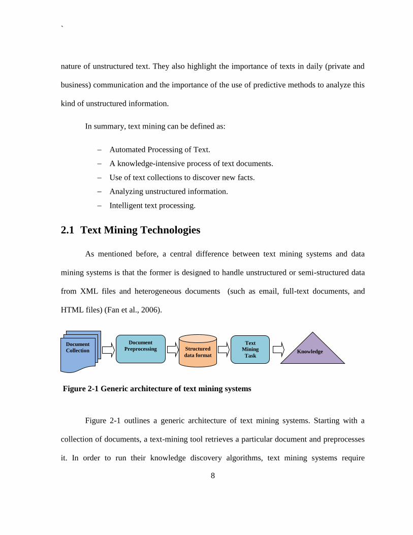
As mentioned before, a central difference between text mining systems and data
mining systems is that the former is designed to handle unstructured or semi-structured data
from XML files and heterogeneous documents (such as email, full-text documents, and
HTML files) (Fan et al., 2006).
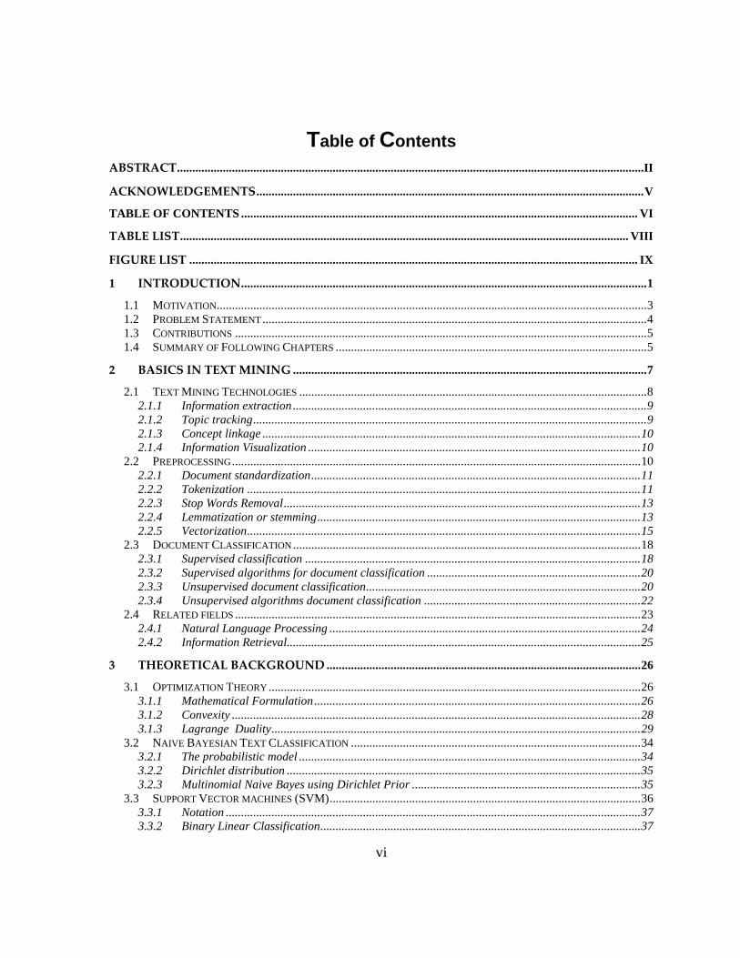
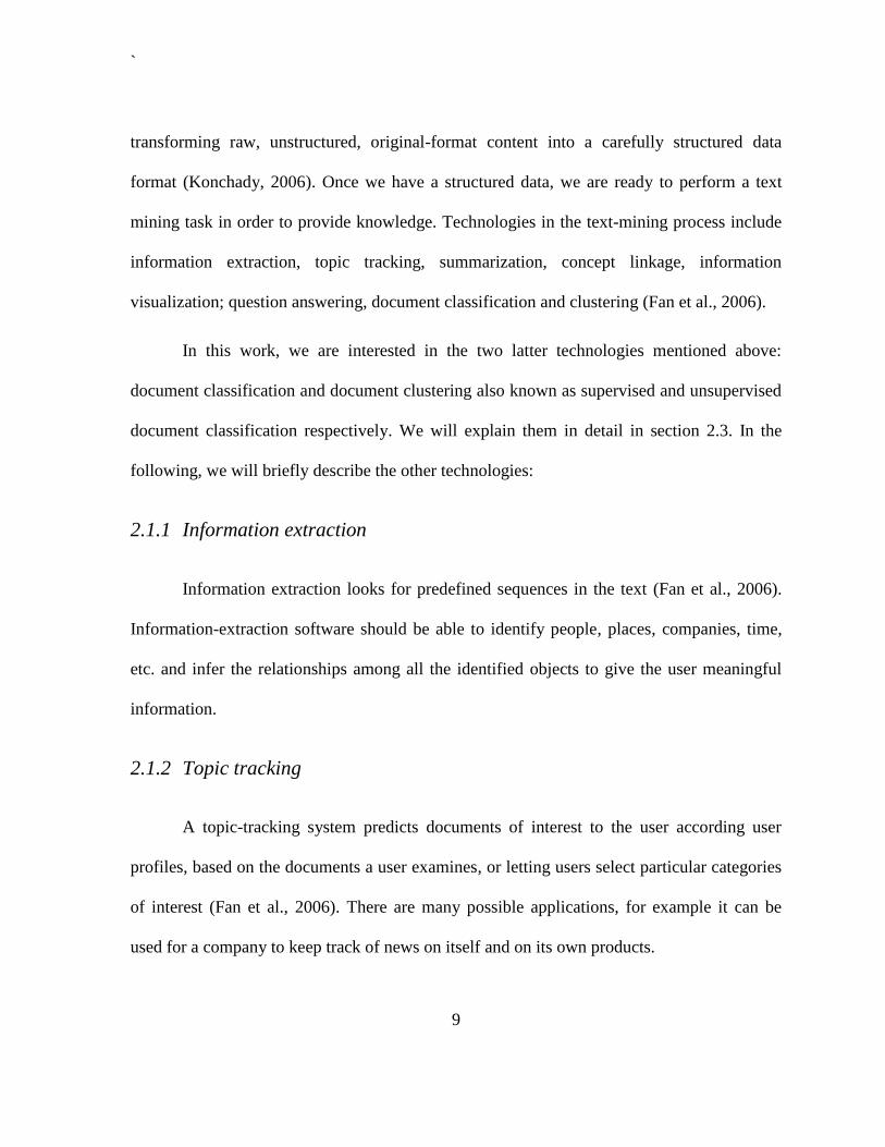
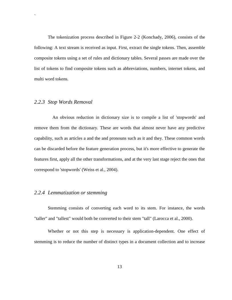
Figure 2-1 Generic architecture of text mining systems
Figure 2-1 outlines a generic architecture of text mining systems. Starting with a
collection of documents, a text-mining tool retrieves a particular document and preprocesses
it. In order to run their knowledge discovery algorithms, text mining systems require
Document
Collection
Document
Preprocessing Structured
data format
Text
Mining
Task Knowledge
`
9
transforming raw, unstructured, original-format content into a carefully structured data
format (Konchady, 2006). Once we have a structured data, we are ready to perform a text
mining task in order to provide knowledge. Technologies in the text-mining process include
information extraction, topic tracking, summarization, concept linkage, information
visualization; question answering, document classification and clustering (Fan et al., 2006).
In this work, we are interested in the two latter technologies mentioned above:
document classification and document clustering also known as supervised and unsupervised
document classification respectively. We will explain them in detail in section 2.3. In the
following, we will briefly describe the other technologies:
2.1.1 Information extraction
Information extraction looks for predefined sequences in the text (Fan et al., 2006).
Information-extraction software should be able to identify people, places, companies, time,
etc. and infer the relationships among all the identified objects to give the user meaningful
information.
2.1.2 Topic tracking
A topic-tracking system predicts documents of interest to the user according user
profiles, based on the documents a user examines, or letting users select particular categories
of interest (Fan et al., 2006). There are many possible applications, for example it can be
used for a company to keep track of news on itself and on its own products.
`
10
2.1.3 Concept linkage
Concept-linkage finds related documents by identifying their shared concepts, helping
users find information they perhaps wouldn‟t have found through traditional search methods
(Fan et al., 2006).
2.1.4 Information Visualization
Information visualization consists in showing large textual sources in a visual
hierarchy or map and providing browsing capabilities, in addition to simple searching (Fan et
al., 2006).
2.2 Preprocessing
Data mining preprocessing focuses on tasks such as normalization, error detection
and correction and dimension reduction. For text mining systems, preprocessing operations
focus on the identification and extraction of representative features for natural language
documents. These preprocessing operations are responsible for transforming unstructured
data stored in document collections into a more explicitly structured intermediate format,
which is a concern that is not relevant for most data mining systems (Feldman et al., 2007).
In the following we will describe the techniques for the transformation of
unstructured text into structured formats.
`
11
2.2.1 Document standardization
Text documents exist in many formats, depending on how the documents were
generated. If we will process all the documents, it is helpful to convert them to a standard
format. Most of the text-processing community, has adopted XML (Extensible Markup
Language) as its standard exchange format (Weiss et al., 2004). Many word processors allow
documents to be saved in XML format, and stand-alone filters can be obtained to convert
existing documents without having to process each one manually (Weiss et al., 2004).
The main advantage of standardizing the data is that the mining tools can be applied
without having to consider the format of the document (Weiss et al., 2004).
2.2.2 Tokenization
The first step in handling text is to break the stream of characters into words or, more
precisely, tokens (Weiss et al., 2004). A token is a more formal definition of a single unit of
text. A single word may not be the smallest unit of text and a token may consist of one or
more words (Feldman et al., 2007).
According to Konchady (Konchady, 2006), a token is a word, number, punctuation
mark, or any other sequence of characters that should be treated as a single unit.
The accurate extraction of tokens is important for precise results in higher-level
applications. Vector representations of documents used in document classification are made
up of a sequence of tokens and weights. Documents can be correctly categorized only when
the vector represents accurately the contents of documents (Konchady, 2006).
`
12
To get the best possible features, one should always customize the tokenizer for the
available text, otherwise extra work may be required after the tokens are obtained. Note that
the tokenization process is language-dependent. In this thesis, we focus on documents in
English. For other languages, although the general principles will be the same, the details
will differ (Weiss et al., 2004).
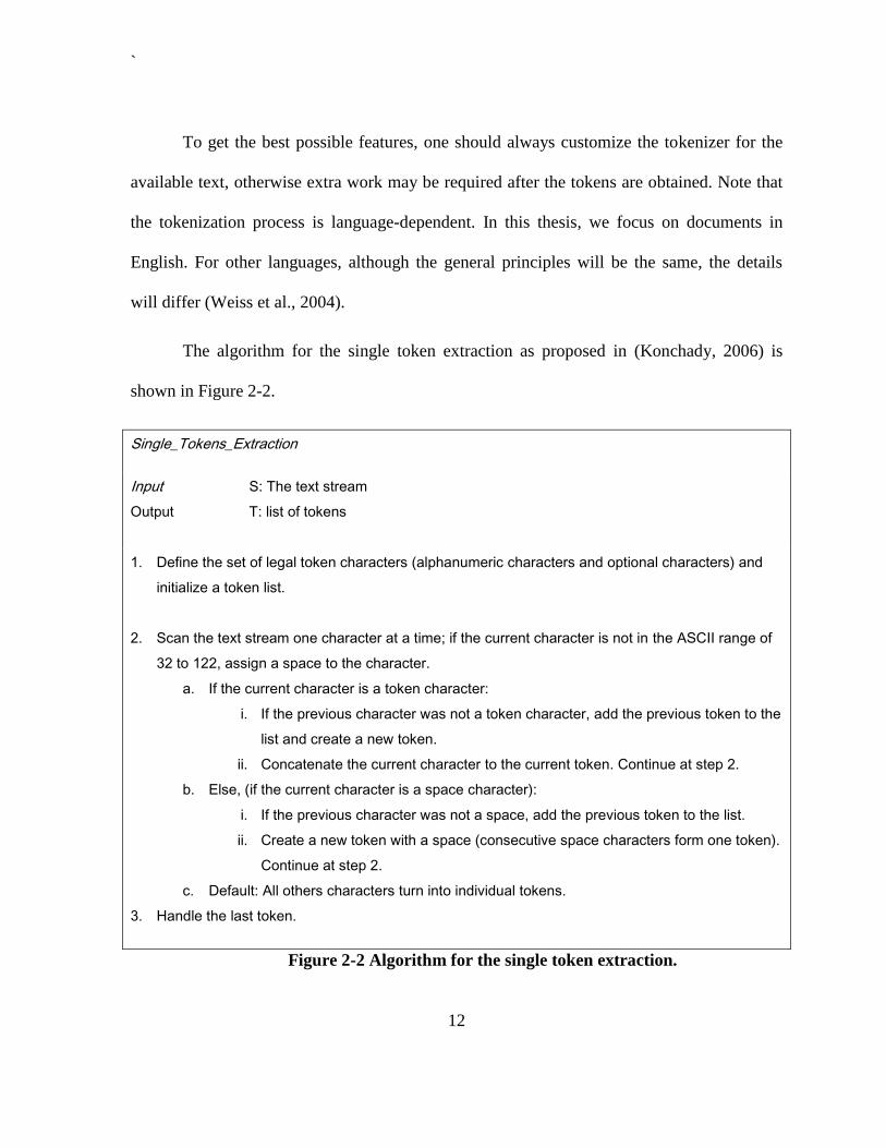
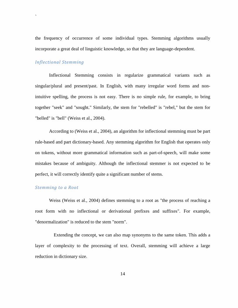
The algorithm for the single token extraction as proposed in (Konchady, 2006) is
shown in Figure 2-2.
Single_Tokens_Extraction
Input
Output
S: The text stream
T: list of tokens
1. Define the set of legal token characters (alphanumeric characters and optional characters) and
initialize a token list.
2. Scan the text stream one character at a time; if the current character is not in the ASCII range of
32 to 122, assign a space to the character.
a. If the current character is a token character:
i. If the previous character was not a token character, add the previous token to the
list and create a new token.
ii. Concatenate the current character to the current token. Continue at step 2.
b. Else, (if the current character is a space character):
i. If the previous character was not a space, add the previous token to the list.
ii. Create a new token with a space (consecutive space characters form one token).
Continue at step 2.
c. Default: All others characters turn into individual tokens.
3. Handle the last token.
Figure 2-2 Algorithm for the single token extraction.
`
13
The tokenization process described in Figure 2-2 (Konchady, 2006), consists of the
following: A text stream is received as input. First, extract the single tokens. Then, assemble
composite tokens using a set of rules and dictionary tables. Several passes are made over the
list of tokens to find composite tokens such as abbreviations, numbers, internet tokens, and
multi word tokens.
2.2.3 Stop Words Removal
An obvious reduction in dictionary size is to compile a list of 'stopwords' and
remove them from the dictionary. These are words that almost never have any predictive
capability, such as articles a and the and pronouns such as it and they. These common words
can be discarded before the feature generation process, but it's more effective to generate the
features first, apply all the other transformations, and at the very last stage reject the ones that
correspond to 'stopwords' (Weiss et al., 2004).
2.2.4 Lemmatization or stemming
Stemming consists of converting each word to its stem. For instance, the words
"taller" and "tallest" would both be converted to their stem "tall" (Larocca et al., 2000).
Whether or not this step is necessary is application-dependent. One effect of
stemming is to reduce the number of distinct types in a document collection and to increase
`
14
the frequency of occurrence of some individual types. Stemming algorithms usually
incorporate a great deal of linguistic knowledge, so that they are language-dependent.
Inflectional Stemming
Inflectional Stemming consists in regularize grammatical variants such as
singular/plural and present/past. In English, with many irregular word forms and non-
intuitive spelling, the process is not easy. There is no simple rule, for example, to bring
together "seek" and "sought." Similarly, the stem for "rebelled" is "rebel," but the stem for
"belled" is "bell" (Weiss et al., 2004).
According to (Weiss et al., 2004), an algorithm for inflectional stemming must be part
rule-based and part dictionary-based. Any stemming algorithm for English that operates only
on tokens, without more grammatical information such as part-of-speech, will make some
mistakes because of ambiguity. Although the inflectional stemmer is not expected to be
perfect, it will correctly identify quite a significant number of stems.
Stemming to a Root
Weiss (Weiss et al., 2004) defines stemming to a root as "the process of reaching a
root form with no inflectional or derivational prefixes and suffixes". For example,
"denormalization" is reduced to the stem "norm".
Extending the concept, we can also map synonyms to the same token. This adds a
layer of complexity to the processing of text. Overall, stemming will achieve a large
reduction in dictionary size.
`
15
2.2.5 Vectorization
Vector based representations has been widely used in text mining process for their
simplicity. They are also referred to as a „bag of words‟, emphasizing that document vectors
are invariant with respect to term permutations, since the original word order in the document
is clearly lost. However, many text retrieval and categorization tasks can be performed quite
well in practice using the vector-space model.
The collective set of tokens or words is typically called a dictionary or vocabulary (V).
They form the basis for creating the numeric vectors corresponding to the document
collection.
More precisely, a text document d can be represented as a sequence of terms,
| | , where |d| is the length of the document and . A vector-space
representation of d is then defined as a real vector | |, where each component is a
statistic related to the occurrence of the vocabulary entry in the document.
Note that typically the total number of terms in a set of documents is much larger than
the number of distinct terms in any single document, |V|>>|d|, so that vector-space
representations tend to be very sparse. This property can be advantageously exploited for
both memory storage and algorithm design.
The simplest vector-based representation is Boolean. In Boolean representation
indicates the presence or the absence of term in the document being
represented.
`
16
Several refinements can be obtained by extending the Boolean vector model and
introducing real-valued weights associated with terms in a document. Other vector-based
representations are described in the next subsections.
Term Frequency
A more informative weighting scheme consists of counting the actual number of
occurrences of each term in the document. This value may be multiplied by the constant
| | to
obtain a vector of term frequencies (TF) within the document.
Let be a collection of documents. For each term , let
denote the number of occurrences of in document . Then we define:
( )
| |
The idea is that terms occurring most often in a document are more relevant than
terms that do not. However, a frequent term may occur in almost every document. Such
terms do not contribute to discriminate between classes. To assign lower weights to such
term, sometimes the document frequency is used. This measure corresponds to the
number of documents in which occurs at least once.
Finally, since documents can be of different length a normalization component
adjusts the weights so that small and large documents can be compared on the same scale.
`
17
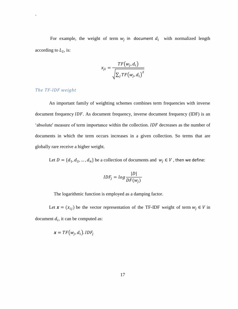
For example, the weight of term in document with normalized length
according to , is:
( )
√∑ ( )
The TF-IDF weight
An important family of weighting schemes combines term frequencies with inverse
document frequency . As document frequency, inverse document frequency (IDF) is an
„absolute' measure of term importance within the collection. decreases as the number of
documents in which the term occurs increases in a given collection. So terms that are
globally rare receive a higher weight.
Let be a collection of documents and , then we define:
| |
The logarithmic function is employed as a damping factor.
Let be the vector representation of the TF-IDF weight of term in
document , it can be computed as:
( )
`
18
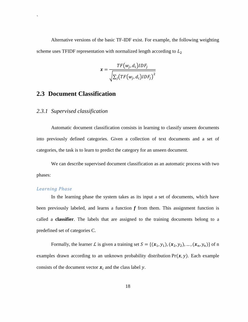
Alternative versions of the basic TF-IDF exist. For example, the following weighting
scheme uses TFIDF representation with normalized length according to
( )
√∑ ( ( ) )
2.3 Document Classification
2.3.1 Supervised classification
Automatic document classification consists in learning to classify unseen documents
into previously defined categories. Given a collection of text documents and a set of
categories, the task is to learn to predict the category for an unseen document.
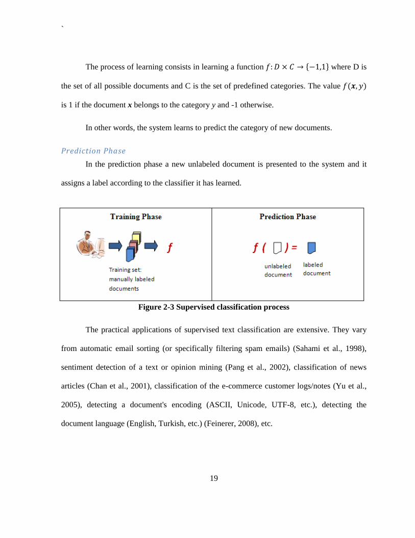
We can describe supervised document classification as an automatic process with two
phases:
Learning Phase
In the learning phase the system takes as its input a set of documents, which have
been previously labeled, and learns a function f from them. This assignment function is
called a classifier. The labels that are assigned to the training documents belong to a
predefined set of categories C.
Formally, the learner is given a training set of n
examples drawn according to an unknown probability distribution . Each example
consists of the document vector and the class label .
`
19
The process of learning consists in learning a function where D is
the set of all possible documents and C is the set of predefined categories. The value
is 1 if the document x belongs to the category y and -1 otherwise.
In other words, the system learns to predict the category of new documents.
Prediction Phase
In the prediction phase a new unlabeled document is presented to the system and it
assigns a label according to the classifier it has learned.
Figure 2-3 Supervised classification process
The practical applications of supervised text classification are extensive. They vary
from automatic email sorting (or specifically filtering spam emails) (Sahami et al., 1998),
sentiment detection of a text or opinion mining (Pang et al., 2002), classification of news
articles (Chan et al., 2001), classification of the e-commerce customer logs/notes (Yu et al.,
2005), detecting a document's encoding (ASCII, Unicode, UTF-8, etc.), detecting the
document language (English, Turkish, etc.) (Feinerer, 2008), etc.
`
20
Supervised text classification algorithms have been successfully used in a wide
variety of practical domains. In experiments conducted by Namburú et al. (Namburú et al.,
2005), using high accuracy classifiers with the most widely used document datasets, they
report up to 96% of accuracy with a binary classification in the Reuters dataset. However,
they needed 2000 manually labeled documents to achieve this good result.
The problem with the supervised learning methods is that they require a large number
of labeled training examples to learn accurately. Manual labeling is a costly and time-
consuming process, since it requires human effort. In some applications, this approach
becomes impractical, since most users would not have time to spend in label thousands of
documents (Nigam, 2001).
2.3.2 Supervised algorithms for document classification
There are many traditional learning methods which have shown good results on text
classification problems in previous studies. Some of them, among others, are the following:
Naïve Bayes classifier (Sahami et al., 1998), k-nearest neighbor classifier, Logistic
Regression, Boosting (Weiss et al., 2004), Support Vector Machines (Joachims, 1998).
2.3.3 Unsupervised document classification
Unsupervised document classification, also known as document clustering, is a
process through which documents are classified into meaningful groups called clusters,
without any prior information. Any labels associated with objects are obtained exclusively
from the data.
`
21
A clustering task may include a definition of proximity or similarity measure suitable
to the domain. There are many possible similarity measures; however, the cosine similarity
measure is the most common for text clustering:
Let x and y vector representations of two documents, and let n the dimension of the
vectors.
∑
where is the normalized vector
‖ ‖ .
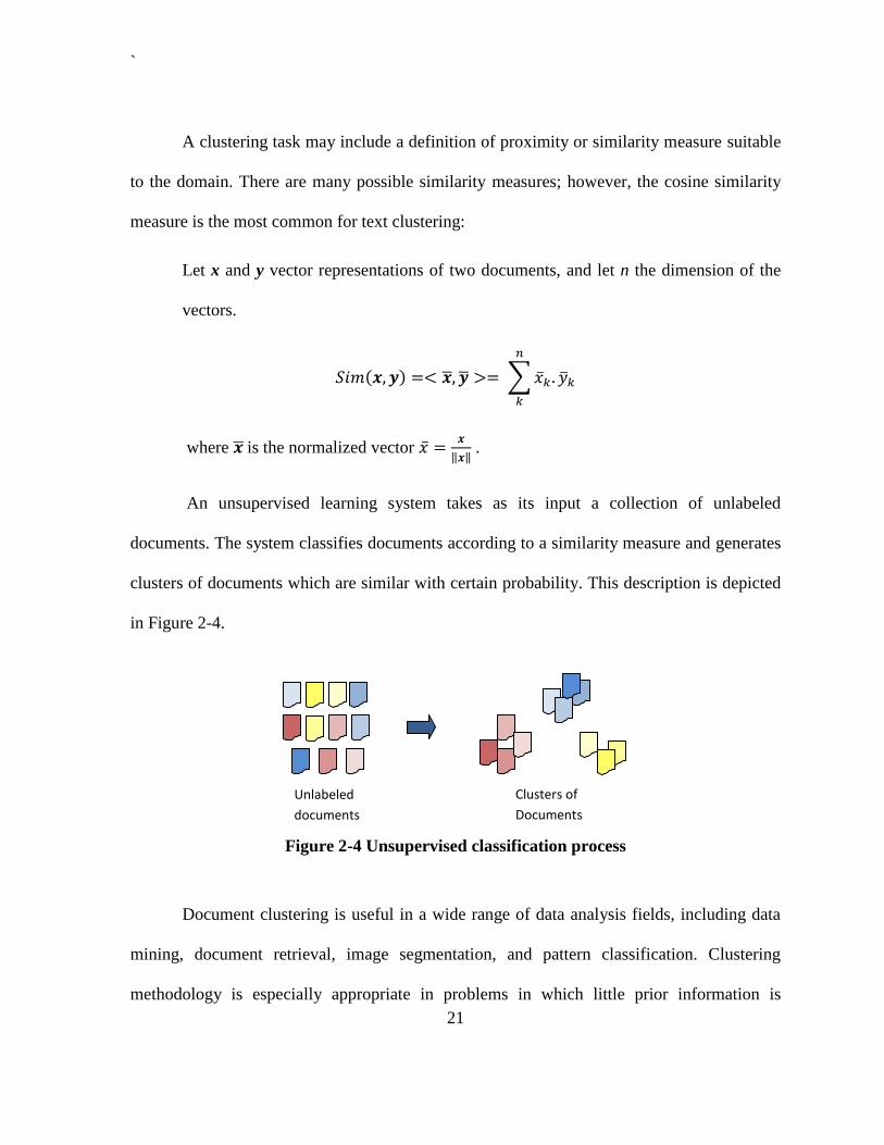
An unsupervised learning system takes as its input a collection of unlabeled
documents. The system classifies documents according to a similarity measure and generates
clusters of documents which are similar with certain probability. This description is depicted
in Figure 2-4.
Figure 2-4 Unsupervised classification process
Document clustering is useful in a wide range of data analysis fields, including data
mining, document retrieval, image segmentation, and pattern classification. Clustering
methodology is especially appropriate in problems in which little prior information is
Unlabeled
documents
Clusters of
Documents
`
22
available and the system must make as few assumptions about the data as possible (Feldman
et al., 2007).
An application of clustering is the analysis and navigation of big text collections such
as Web pages. The basic assumption, called the cluster hypothesis, states that relevant
documents tend to be more similar to each other than to non-relevant ones. If this assumption
holds for a particular document collection, the clustering of documents based on the
similarity of their content may help to improve the search effectiveness (Feldman et al.,
2007).
2.3.4 Unsupervised algorithms document classification
Traditionally clustering techniques are divided in hierarchical and partitioning
(Berkhin, 2002). Each of these can either be a hard clustering or a soft one. In a hard
clustering, every object may belong to exactly one cluster. In soft clustering, the membership
is fuzzy, objects may belong to several clusters with a fractional degree of membership in
each (Feldman et al., 2007).
Hierarchical algorithms build clusters gradually. The basics of hierarchical
clustering include the idea of conceptual clustering. Classic algorithms SLINK (Single
LINKage), COBWEB, as well as newer algorithms CURE (Clustering Using
Representatives) and CHAMELEON are in this category.
Partitioning algorithms learn clusters directly. In doing so, they either try to
discover clusters by iteratively relocating points between subsets (Partitioning Relocation

`
23
Methods), or try to identify clusters as areas highly populated (Density-Based Partitioning).
Partitioning Relocation Methods are further categorized into probabilistic clustering (EM
(Expectation Maximization), framework algorithms (SNOB, AUTOCLASS, MCLUST), k-
medoids methods like algorithms (Kaufman and Rousseeuw) PAM (Partitioning Around
Medoids), CLARA (Clustering LARge Applications), CLARANS (clustering Large
Application based upon Randomized Search) and its extensions, and k-means methods
(different schemes initialization, optimization, harmonic means, extensions). Such methods
concentrate on how well points fit into their clusters and tend to build clusters of proper
convex shapes.
Many other clustering techniques are developed, that work well in particular
scenarios. The most commonly used algorithms are the K-means, the EM-based mixture
resolving (soft, flat, probabilistic), and the HAC (hierarchical, agglomerative).
The clustering of textual data has several unique features that distinguish it from
other clustering problems. The most prominent feature of text documents as objects to be
clustered is their very complex and rich internal structure. With big document collections, the
dimension of the feature space may easily range into the tens and hundreds of thousands.
2.4 Related fields
There is a huge amount of contributions that underlines the cross-disciplinary
research in text mining with connections to various related fields, like statistics, computer
`
24
science, or linguistics. In the following we will describe those which, we consider, are the
most important:
2.4.1 Natural Language Processing
Text mining aims to extract or generate new information from textual information but
does not necessarily need to understand the text itself. Instead, natural language processing
tries to obtain a thorough impression on the language structure within texts. This allows a
deeper analysis of sentence structures, grammar, morphology, and thus better retrieves the
latent semantic structure inherent to texts (Feinerer, 2008). Some applications of natural
language processing closely related to text mining are:
Automatic Summarization
Summarization reduces the length and detail of a document while retaining its main
points and overall meaning (Fan et al., 2006). Text summarization helps users figure out
whether a lengthy document meets their needs and is worth reading.
Question answering
Another application area of natural language processing is natural language queries,
or question answering (QandA), which deals with how to find the best answer to a given
question (Fan et al., 2006).
`
25
2.4.2 Information Retrieval
Information retrieval (IR) is concerned with searching for documents, for information
within documents, and for metadata about documents, as well as that of searching relational
databases and the World Wide Web.
Automated information retrieval systems are used to reduce overload of information.
Many universities and public libraries use IR systems to provide access to books, journals
and other documents. Web search engines are the most visible IR applications.
`
26
3 THEORETICAL BACKGROUND
In this chapter, we review the main theoretical fundamentals in which we base our
thesis. We also provide a review of early work related to this thesis.
Section 1 introduces the optimization theory which is a fundamental block in the
construction of Support Vector Machines. Section 2 introduces the naive Bayesian
classification for text documents. Section 3 introduces the traditional Support Vector
Machines applied to text documents. In Section 4 we give an overview of early work in semi-
supervised document classification. Finally, section 5 introduces the concept of Ontology.
3.1 Optimization Theory
Optimization theory is the branch of mathematics that studies the extremal values of a
function. It is concerned with determining the most profitable or least disadvantageous
solution out of a set of alternatives and developing effective algorithms for finding them.
Typically the set of alternatives is restricted by several constraints on the values of a number
of variables and an objective function locates the optimum in the remaining set.
3.1.1 Mathematical Formulation
Optimization is the minimization or maximization of a function subject to constraints
on its variables (Nocedal et al., 1999).
The general optimization problem can be stated as follows:
`
27
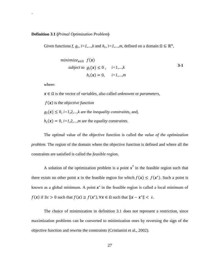
Definition 3.1 (Primal Optimization Problem)
Given functions f, , i=1,...,k and , i=1,...,m, defined on a domain ,
subject to , i=1,...,k 3-1
, i=1,...,m
where:
is the vector of variables, also called unknowns or parameters,
is the objective function
, i=1,2,...,k are the inequality constraints, and,
, i=1,2,...,m are the equality constraints.
The optimal value of the objective function is called the value of the optimization
problem. The region of the domain where the objective function is defined and where all the
constraints are satisfied is called the feasible region.
A solution of the optimization problem is a point x* in the feasible region such that
there exists no other point x in the feasible region for which . Such a point is
known as a global minimum. A point in the feasible region is called a local minimum of
if such that such that ‖ ‖ .
The choice of minimization in definition 3.1 does not represent a restriction, since
maximization problems can be converted to minimization ones by reversing the sign of the
objective function and rewrite the constraints (Cristianini et al., 2002).
`
28
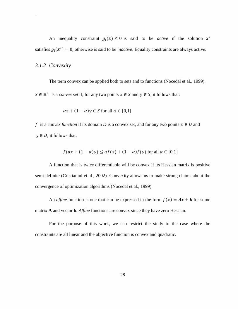
An inequality constraint is said to be active if the solution
satisfies , otherwise is said to be inactive. Equality constraints are always active.
3.1.2 Convexity
The term convex can be applied both to sets and to functions (Nocedal et al., 1999).
is a convex set if, for any two points and , it follows that:
for all [ ]
is a convex function if its domain D is a convex set, and for any two points and
y , it follows that:
for all [ ]
A function that is twice differentiable will be convex if its Hessian matrix is positive
semi-definite (Cristianini et al., 2002). Convexity allows us to make strong claims about the
convergence of optimization algorithms (Nocedal et al., 1999).
An affine function is one that can be expressed in the form for some
matrix A and vector b. Affine functions are convex since they have zero Hessian.
For the purpose of this work, we can restrict the study to the case where the
constraints are all linear and the objective function is convex and quadratic.
`
29
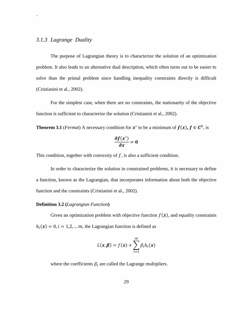
3.1.3 Lagrange Duality
The purpose of Lagrangian theory is to characterize the solution of an optimization
problem. It also leads to an alternative dual description, which often turns out to be easier to
solve than the primal problem since handling inequality constraints directly is difficult
(Cristianini et al., 2002).
For the simplest case, when there are no constraints, the stationarity of the objective
function is sufficient to characterize the solution (Cristianini et al., 2002).
Theorem 3.1 (Fermat) A necessary condition for to be a minimum of , , is
This condition, together with convexity of , is also a sufficient condition.
In order to characterize the solution in constrained problems, it is necessary to define
a function, known as the Lagrangian, that incorporates information about both the objective
function and the constraints (Cristianini et al., 2002).
Definition 3.2 (Lagrangian Function)
Given an optimization problem with objective function , and equality constraints
, the Lagrangian function is defined as
∑
where the coefficients are called the Lagrange multipliers.
`
30
If a point is a local minimum of , , for a problem with only equality
constraints, it is possible that
, but the directions in which we could move to reduce
cause us to violate one or more of the constraints (Cristianini et al., 2002). In order to
respect the equality constraint , we must move perpendicular to
, and so to respect all
of the equality constraints we must move perpendicular to the subspace V spanned by
{
}
if the
are linearly independent no legal move can change the value of the
objective function, whenever
lies in the subspace , or in other words when there
exists such that
∑
Theorem 3.2 (Lagrange)
A necessary condition for a normal point to be a minimum of , subject to
, with , is
for some values . The above conditions are also sufficient provided that is
a convex function of x.
`
31
The first of the 2 conditions gives a new system of equations, whereas the second
condition returns the equality constraints. By jointly solving the two systems one obtain the
solution.
Definition 3.3 (Generalized Lagrangian function)
Given an optimization problem defined on a domain ,
subject to , i=1,...,k
, i=1,...,m
the Generalized Lagrangian function is defined as
∑
∑
where the coefficients and are called the Lagrange multipliers.
Definition 3.4 (Lagrangian dual problem)
The Lagrangian dual problem of the primal problem of Definition 3.1 is the
following problem:
subject to , 3-2
where .
Lagrange multipliers are also called dual variables.
`
32
Theorem 3.3 (Weak duality)
Let be a feasible solution of the primal problem of Definition 3.1 and a
feasible solution of the dual problem of Definition 3.4. Then . (Cristianini et
al., 2002)
Corollary 3.1
The value of the dual is upper bounded by the value of the primal.
Corollary 3.2
If , where and ,
, then and solve
the primal and dual problem respectively. In this case
, for i=1,...,k.
The solutions of the primal and dual having the same value is not in general
guaranteed. The difference between the values of the primal and the dual problems is known
as the duality gap.
Theorem 3.4 (Strong duality)
Given an optimization problem with convex domain ,
subject to , i=1,...,k
, i=1,...,m
where and are affine functions, that is for some matrix A and
some vector b, then the duality gap is zero.
`
33
Theorem 3.5 (Kuhn-Tucker)
Given an optimization problem with convex domain ,
subject to , i=1,...,k
, i=1,...,m
with convex and and affine, necessary and sufficient conditions for a
point to be an optimum are the existence of such that:
(Karush-Kuhn-Tucker (KKT) conditions)
The third relation is known as the Karush-Kuhn-Tucker (KKT) complementary
condition. It implies that for inactive constraints, . Perturbing inactive constraints has
no effect on the solution of the optimization problem.
We can transform the primal problem into its corresponding dual by setting to zero
the derivatives of the Lagrangian with respect to the primal variables, and substituting the
resulting relations back into the Lagrangian. In this way we remove the dependence of the
`
34
primal variables. The resulting function contains only dual variables and must be maximized
under simpler constraints (Cristianini et al., 2002).
3.2 Naive Bayesian Text Classification
3.2.1 The probabilistic model
In order to model the data, Naïve Bayes classifiers assume that documents are
generated by a mixture of multinomial distributions model, where each mixture component
corresponds to a class.
Bayes‟ rule says that to achieve the highest classification accuracy, a document
should be assigned to the class for which | is highest.
Suppose that C is the number of classes, the vocabulary is of size |V|, and each
document di has |di| words in it.
The likelihood of seeing document di is a sum of total probability over all mixture
components. That is,
| ∑ ( | ) ( | )
3-3
Using the above along with standard Naive Bayes assumption: that the words of a
document are conditionally independent among them, given the class label, we can expand
the second term of equation 3-3, and express the probability of a document given a mixture
`
35
component in terms of its constituent features: the document length and the words in the
document.
( | ) | | ∏ |
3-4
Where refers to the number of times word wt occurs in document di.
The full generative model, given by combining equations 3-3 and 3-4, assigns
probability P(di|Ө) to generate document di as follows:
| | | ∑ |
∏ |
3-5
3.2.2 Dirichlet distribution
Let a random vector such that ∑ .
The Dirichlet distribution with parameters is given by:
| ∑
∏ ∏
3-6
Where an with large components correspond to strong prior knowledge about the
distribution and with small components correspond to ignorance.
3.2.3 Multinomial Naive Bayes using Dirichlet Prior
Using maximum a posteriori (MAP) to estimate the parameters of a multinomial
distribution with Dirichlet prior, yields:
`
36
| |
∑ | |
| | ∑ ∑ | |
| |
3-7
|
∑ | |
| | 3-8
Given estimates of these parameters, it is possible to calculate the probability that a
particular mixture component generated a given document to perform classification. By
applying Bayes rule it follows that:
( | ) | ∏ |
∑ | ∏ |
3-9
Then, to classify a test document into a single class, the class with the highest
posterior probability is selected. See more details in (Mitchel, 2005).
3.3 Support Vector machines (SVM)
The learning method of Support Vector Machines (SVM) was introduced by Vladimir
Vapnik et al (Boser et al., 1992). Supervised support vector machine technique has been
successfully used in text domains (Joachims, 1998).
Support Vector Machines is a system for efficiently training linear learning machines
in kernel-induced feature spaces. Linear learning machines are learning machines that form
linear combinations of the input variables (Cristianini et al., 2002).
`
37
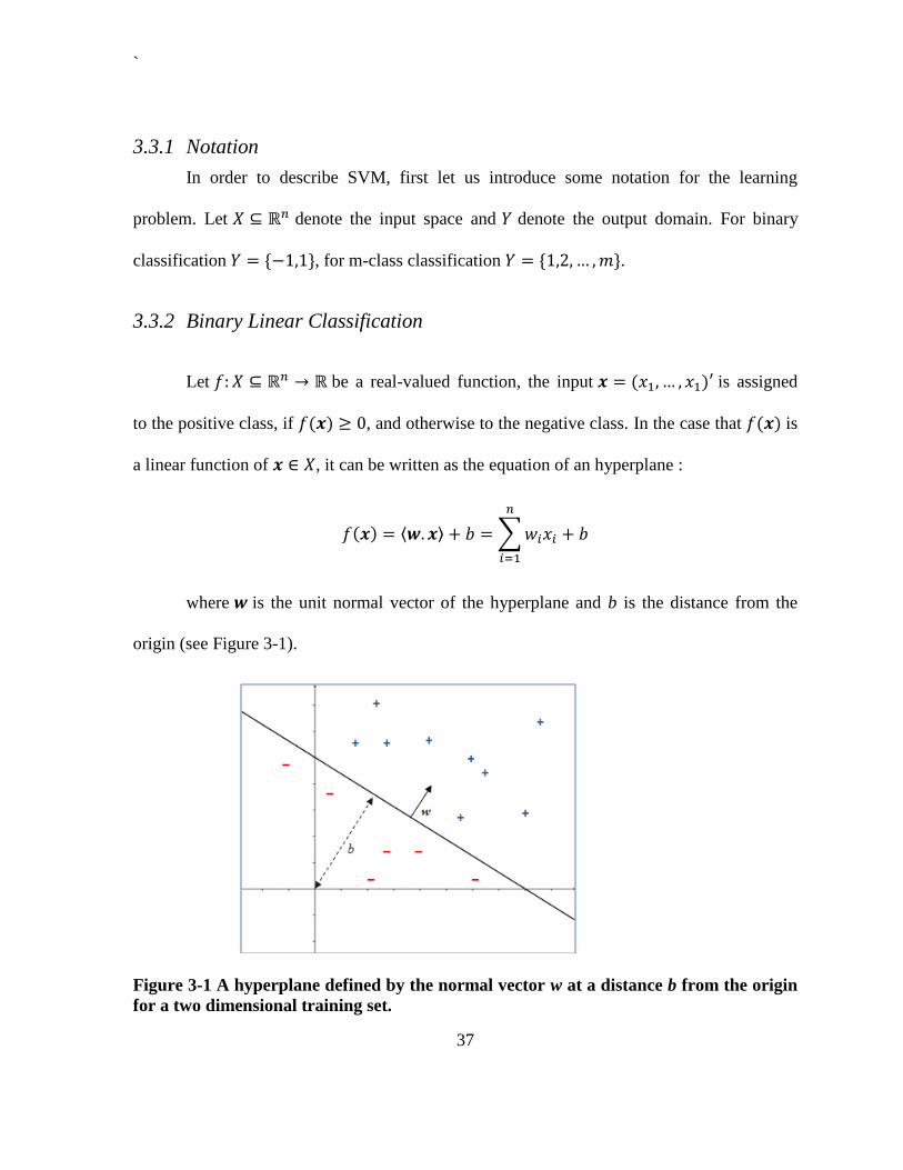
3.3.1 Notation
In order to describe SVM, first let us introduce some notation for the learning
problem. Let denote the input space and denote the output domain. For binary
classification , for m-class classification .
3.3.2 Binary Linear Classification
Let be a real-valued function, the input is assigned
to the positive class, if , and otherwise to the negative class. In the case that is
a linear function of , it can be written as the equation of an hyperplane :
⟨ ⟩ ∑
where is the unit normal vector of the hyperplane and b is the distance from the
origin (see Figure 3-1).
Figure 3-1 A hyperplane defined by the normal vector w at a distance b from the origin
for a two dimensional training set.
`
38
Then, the decision rule is given by . The parameters that control the
learning function and must be learned from the data are . The hyperplane
defined by the function above is called the decision boundary.
The quantities and b are usually called the weight vector and bias, respectively.
Sometimes b is replaced by and is called threshold (Cristianini et al., 2002).
If there exists a hyperplane that correctly classifies the training data, we say that the
data are linearly separable. If no such hyperplane exists the data are said to be nonseparable.
Intuitively, we can see that if a point is far from the separating hyperplane, then we may be
significantly more confident in the prediction for the value of y at this point. And, for a given
training set, it would be good if we manage to find a decision boundary that allows us to
make all correct and confident predictions on the training examples (meaning far from the
decision boundary). We will formalize this later using the concepts of margins.
3.3.3 Geometric and Functional Margins
Geometric Margin
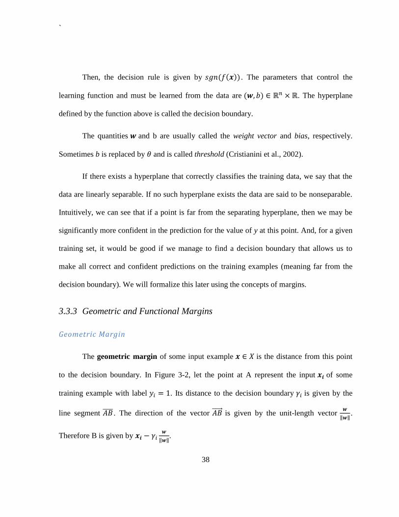
The geometric margin of some input example is the distance from this point
to the decision boundary. In Figure 3-2, let the point at A represent the input of some
training example with label . Its distance to the decision boundary is given by the
line segment . The direction of the vector is given by the unit-length vector
‖ ‖.
Therefore B is given by
‖ ‖.
`
39
Figure 3-2 Geometric margin of an input example.
Since B lies on the decision boundary then it satisfies the equation:
⟨ ⟩
Hence,
(
‖ ‖)
‖ ‖
‖ ‖
‖ ‖
‖ ‖
‖ ‖
‖ ‖
Making the analogous process for the case of a negative example we get:
`
40
(
‖ ‖
‖ ‖)
In general, we define the geometric margin of an hyperplane with respect to a
training example ( to be
(
‖ ‖
‖ ‖) 3-10
It is worth noting that the geometric margin is invariant to rescaling of the parameters
to . This fact will be useful later.
Finally, giving a training set , we define the geometric
margin of an hyperplane with respect to S to be the smallest of the geometric margins
on the individual training examples.
Functional Margin
We define the functional margin of an hyperplane with respect to a training
example ( to be the quantity:
(3-11)
If , then for the functional margin to be large, and in consequence, for our
prediction to be confident and correct, we need to be a large positive number. In
the other hand, if , then for the functional margin to be large, we need to
be a large negative number. Furthermore, implies correct classification of ( .
Thus, a large functional margin represents a confident and a correct prediction.
`
41
Since the geometric margin equals the functional margin when ‖ ‖ , thus
geometrical and functional margin are related by
‖ ‖.
Note that in the definition of linear classifiers there is an inherent degree of freedom,
due to the fact that the function associated with the hyperplane does not change if we
rescale the hyperplane to . There will, however, be a change in the
(functional) margin as measured by the function output as opposed to the geometric margin
(Cristianini et al., 2002).
The functional margin distribution of a hyperplane with respect to a training
set , is the distribution of the margins of the examples in S. We
refer to the minimum of the functional margin distribution as the functional margin of a
hyperplane with respect to a training set S.
3.3.4 The Maximal Margin Classifier
The maximal margin classifier is the simplest model of Support Vector Machine. It
tries to find a decision boundary that maximizes the geometric margin, since this would
reflect very confident predictions on the training set. For this model, we assume that the
training data are linearly separable.
Since we are trying to maximize the geometrical margin
‖ ‖ , we can pose the
following optimization problem:
`
42
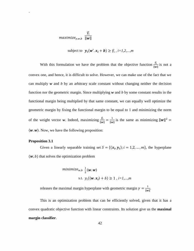
‖ ‖
subject to , i=1,2,...,m
With this formulation we have the problem that the objective function
‖ ‖ is not a
convex one, and hence, it is difficult to solve. However, we can make use of the fact that we
can multiply w and b by an arbitrary scale constant without changing neither the decision
function nor the geometric margin. Since multiplying w and b by some constant results in the
functional margin being multiplied by that same constant, we can equally well optimize the
geometric margin by fixing the functional margin to be equal to 1 and minimizing the norm
of the weight vector w. Indeed, maximizing
‖ ‖
‖ ‖ is the same as minimizing ‖ ‖
⟨ ⟩. Now, we have the following proposition:
Proposition 3.1
Given a linearly separable training set , the hyperplane
that solves the optimization problem
⟨ ⟩
s.t. ⟨ ⟩ , i=1,...,m
releases the maximal margin hyperplane with geometric margin
‖ ‖.
This is an optimization problem that can be efficiently solved, given that it has a
convex quadratic objective function with linear constraints. Its solution give us the maximal
margin classifier.
`
43
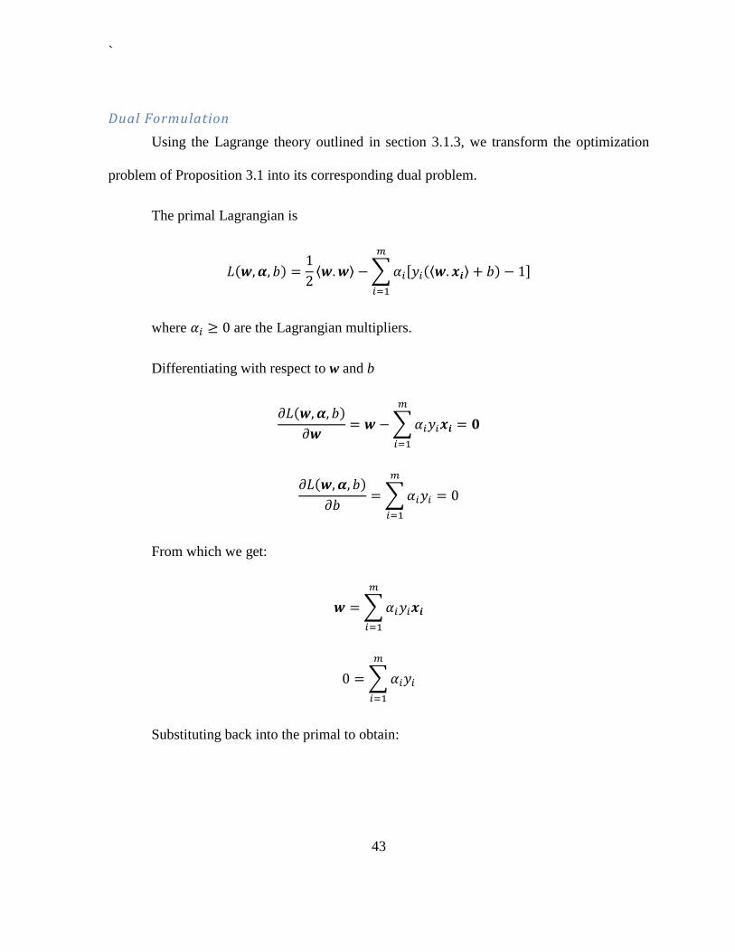
Dual Formulation
Using the Lagrange theory outlined in section 3.1.3, we transform the optimization
problem of Proposition 3.1 into its corresponding dual problem.
The primal Lagrangian is
⟨ ⟩ ∑ [ ⟨ ⟩ ]
where are the Lagrangian multipliers.
Differentiating with respect to w and b
∑
∑
From which we get:
∑
∑
Substituting back into the primal to obtain:
`
44
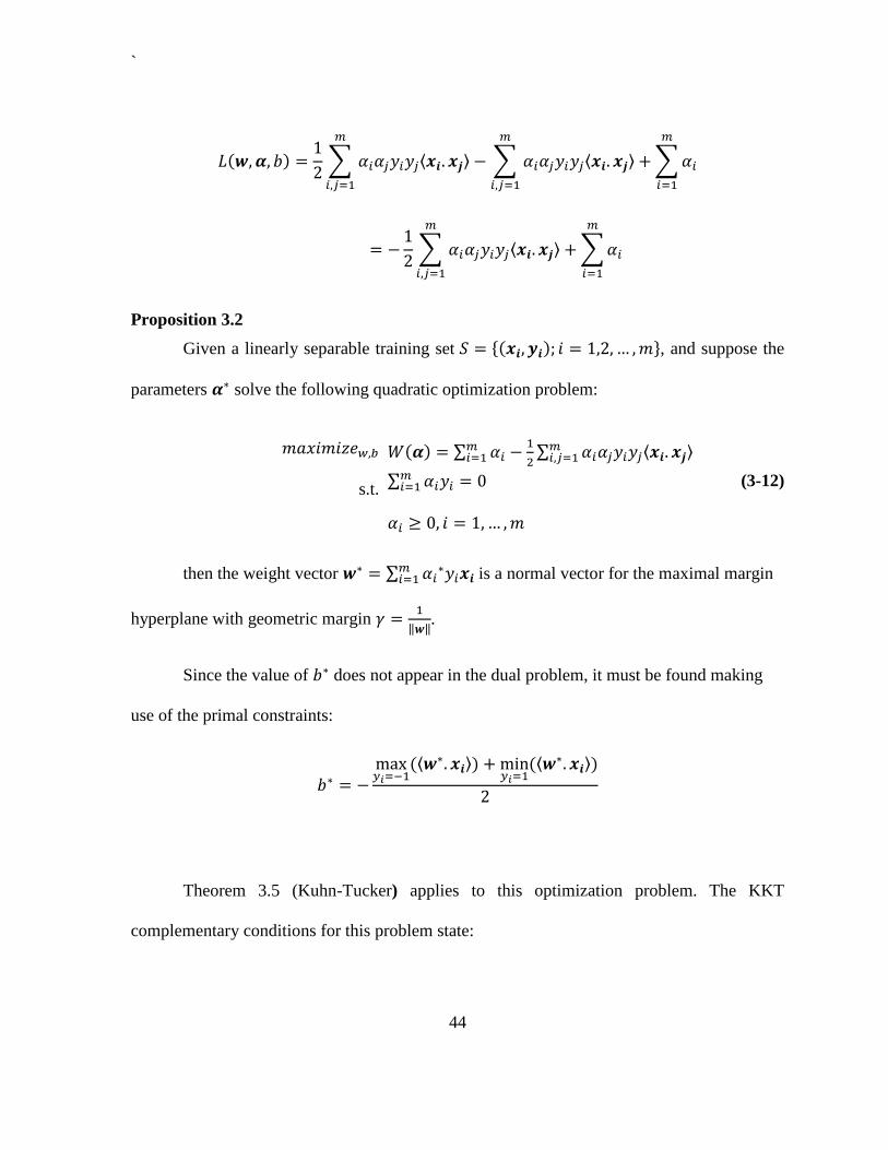
∑ ⟨ ⟩
∑ ⟨ ⟩
∑
∑ ⟨ ⟩
∑
Proposition 3.2
Given a linearly separable training set , and suppose the
parameters solve the following quadratic optimization problem:
∑
∑ ⟨ ⟩
s.t. ∑
(3-12)
then the weight vector ∑
is a normal vector for the maximal margin
hyperplane with geometric margin
‖ ‖.
Since the value of does not appear in the dual problem, it must be found making
use of the primal constraints:
⟨ ⟩
⟨ ⟩
Theorem 3.5 (Kuhn-Tucker) applies to this optimization problem. The KKT
complementary conditions for this problem state:
`
45
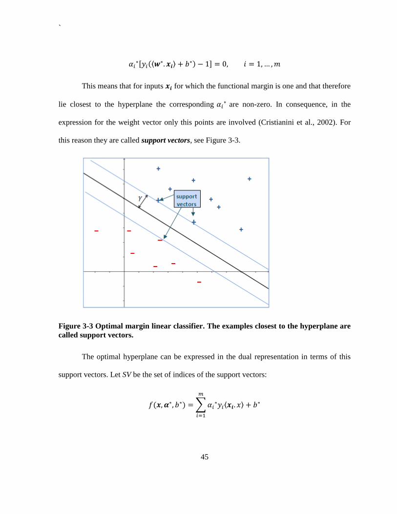
[ ⟨
⟩ ]
This means that for inputs for which the functional margin is one and that therefore
lie closest to the hyperplane the corresponding are non-zero. In consequence, in the
expression for the weight vector only this points are involved (Cristianini et al., 2002). For
this reason they are called support vectors, see Figure 3-3.
Figure 3-3 Optimal margin linear classifier. The examples closest to the hyperplane are
called support vectors.
The optimal hyperplane can be expressed in the dual representation in terms of this
support vectors. Let SV be the set of indices of the support vectors:
∑ ⟨ ⟩
`
46
∑ ⟨ ⟩
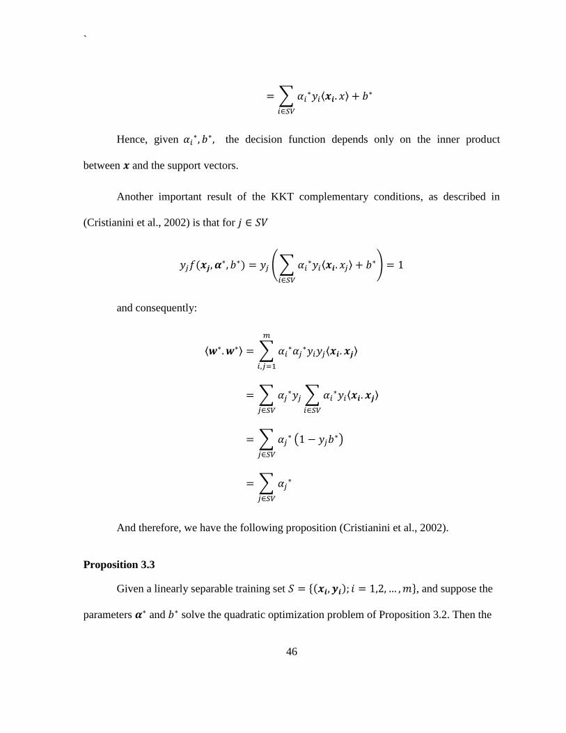
Hence, given the decision function depends only on the inner product
between and the support vectors.
Another important result of the KKT complementary conditions, as described in
(Cristianini et al., 2002) is that for
(∑
⟨ ⟩
)
and consequently:
⟨ ⟩ ∑
⟨ ⟩
∑
∑ ⟨ ⟩
∑
( )
∑
And therefore, we have the following proposition (Cristianini et al., 2002).
Proposition 3.3
Given a linearly separable training set , and suppose the
parameters and solve the quadratic optimization problem of Proposition 3.2. Then the
`
47
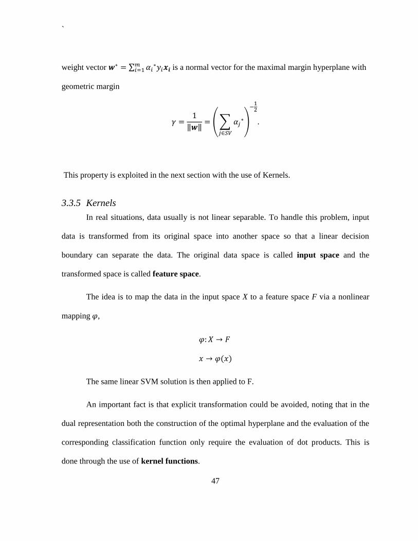
weight vector ∑
is a normal vector for the maximal margin hyperplane with
geometric margin
‖ ‖ (∑
)
This property is exploited in the next section with the use of Kernels.
3.3.5 Kernels
In real situations, data usually is not linear separable. To handle this problem, input
data is transformed from its original space into another space so that a linear decision
boundary can separate the data. The original data space is called input space and the
transformed space is called feature space.
The idea is to map the data in the input space X to a feature space F via a nonlinear
mapping ,
The same linear SVM solution is then applied to F.
An important fact is that explicit transformation could be avoided, noting that in the
dual representation both the construction of the optimal hyperplane and the evaluation of the
corresponding classification function only require the evaluation of dot products. This is
done through the use of kernel functions.
`
48
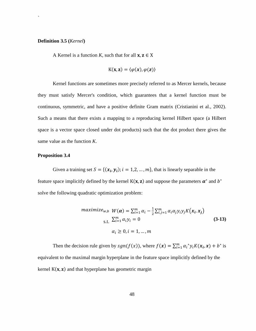
Definition 3.5 (Kernel)
A Kernel is a function K, such that for all
⟨ ⟩
Kernel functions are sometimes more precisely referred to as Mercer kernels, because
they must satisfy Mercer's condition, which guarantees that a kernel function must be
continuous, symmetric, and have a positive definite Gram matrix (Cristianini et al., 2002).
Such a means that there exists a mapping to a reproducing kernel Hilbert space (a Hilbert
space is a vector space closed under dot products) such that the dot product there gives the
same value as the function K.
Proposition 3.4
Given a training set , that is linearly separable in the
feature space implicitly defined by the kernel and suppose the parameters and
solve the following quadratic optimization problem:
∑
∑ ( )
s.t. ∑
(3-13)
Then the decision rule given by , where ∑
is
equivalent to the maximal margin hyperplane in the feature space implicitly defined by the
kernel and that hyperplane has geometric margin
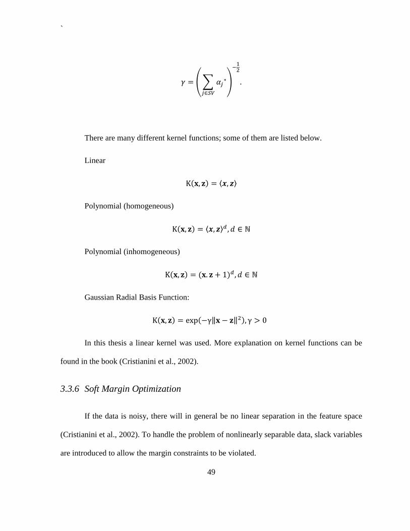
`
49
(∑
)
There are many different kernel functions; some of them are listed below.
Linear
⟨ ⟩
Polynomial (homogeneous)
⟨ ⟩
Polynomial (inhomogeneous)
Gaussian Radial Basis Function:
‖ ‖
In this thesis a linear kernel was used. More explanation on kernel functions can be
found in the book (Cristianini et al., 2002).
3.3.6 Soft Margin Optimization
If the data is noisy, there will in general be no linear separation in the feature space
(Cristianini et al., 2002). To handle the problem of nonlinearly separable data, slack variables
are introduced to allow the margin constraints to be violated.
`
50
2-norm Soft Margin
This approach consists in solving the generalized optimal plane (GOP) problem
(Bennett et al., 1998) given by:
∑
‖ ‖
3-14
Where is a penalty parameter. For each point, is added a slack term such that
if the point is misclassified, .
1-norm Soft Margin
A Robust Linear Programming approach is presented in (Bennett, 1992). It considers
the use of the 1-norm instead of the 2-norm, ‖ ‖ ∑ | | . The problem becomes the
following optimization problem:
∑
∑
3-15
`
51
3.3.7 Multiclass discrimination
We can also solve the problem of binary classification by defining a weight vector
and bias for each class (Cristianini et al., 2002). When a new instance x has to be
classified, both functions are evaluated, and the point x is assigned to class 1 if ⟨ ⟩
⟨ ⟩ , otherwise x is assigned to class -1. This approach is equivalent to
discrimination using the single hyperplane ( ) (Cristianini et al., 2002).
This approach could be used for multiclass discrimination with output domain
. For each class, define a weight vector and bias , and the decision
function is given by
⟨ ⟩
This is equivalent to associating a hyperplane to each class, and to assigning a new
point x to the class whose hyperplane is furthest from it (Cristianini et al., 2002).
3.4 Semi-supervised Document Classification
The general idea of semi-supervised learning is to use a small number of labeled
examples and a large number of unlabeled examples to achieve high-accuracy classification.
The motivation for the use of unlabeled documents for text classification is that we have
many electronic documents readily available. But, labeling the documents must typically be
done by a person, which is a costly and time-consuming process. Nigam et al. showed that, in
certain circumstances, it is possible to train a system using both unlabeled and labeled
`
52
documents and explained why unlabeled data could benefit the classification task (Nigam,
2001).
3.4.1 The value of unlabeled data
An intuitive idea given by Nigam can make us understand why unlabeled data can be
helpful. "Suppose we have some web pages about academic courses, along with a large
number of web pages that are unlabeled. By looking at just the labeled data we determine
that pages containing the word homework tend to be about academic courses. If we use this
fact to estimate the classification of the many unlabeled web pages, we might find that the
word lecture occurs frequently in the unlabeled examples that are now believed to belong to
the positive class. This co-occurrence of the words homework and lecture over the large set
of unlabeled training data can provide useful information to construct a more accurate
classifier that considers both homework and lecture as indicators of positive examples"
(Nigam, 2001).
3.4.2 Semi-supervised Expectation Maximization with Naive Bayes
The model considered in (Nigam, 2001) uses an algorithm for learning from labeled
and unlabeled documents based on the combination of Expectation-Maximization (EM) and
the naive Bayes classifier.
When we have unlabeled data available, we would still like to find MAP parameter
estimates, as in the supervised setting above. Using the Expectation-Maximization (EM)
technique, we can find locally MAP parameter estimates for the generative model.
`
53
The probability of an individual unlabeled document is a sum of total probability over
all the classes, as in equation 3-3. Hence, the expected log probability of the data, containing
|D|, is:
| ∑
| |
∑ | ( | )
3-16
The Expectation-Maximization (EM) is a two-step process that provides an iterative
approach to finding a local maximum of model probability in parameter space. The E-step of
the algorithm estimates the expectations of the class given the latest iteration of the model
parameters. The M-step maximizes the likelihood of the model parameters using the
previously computed expectations of the missing values as if they were the true ones.
In practice, the E-step corresponds to performing classification of each unlabeled
document using equation 3-9. The M-step corresponds to calculating a new maximum a
posteriori estimate for the parameters, using Equations 3-7 and 3-8 with the current estimates.
This algorithm is guaranteed to converge to some local maxima. The algorithm
iterates until it converges to a point where the parameters does not change from one iteration
to the next.
For the semi-supervised case, we consider using a limited number of labeled data in
the initialization step. We first train a classifier using the labeled data, and then estimate the
parameters. After that, the algorithm iterates trying to improve the log likelihood of the data.
The algorithm for the semi-supervised document classification is shown in Figure 3-4.
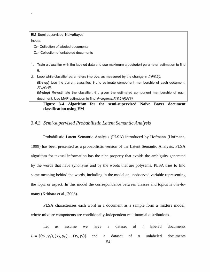
`
54
EM_Semi-supervised_NaiveBayes
Inputs:
Dl= Collection of labeled documents
Du= Collection of unlabeled documents
1. Train a classifier with the labeled data and use maximum a posteriori parameter estimation to find
θ.
2. Loop while classifier parameters improve, as measured by the change in l θ|D Y
(E-step) Use the current classifier, θ , to estimate component membership of each document,
P(cj|Di θ
(M-step) Re-estimate the classifier, θ , given the estimated component membership of each
document. Use MAP estimation to find θ θ D Y|θ θ
Figure 3-4 Algorithm for the semi-supervised Naïve Bayes document
classification using EM
3.4.3 Semi-supervised Probabilistic Latent Semantic Analysis
Probabilistic Latent Semantic Analysis (PLSA) introduced by Hofmann (Hofmann,
1999) has been presented as a probabilistic version of the Latent Semantic Analysis. PLSA
algorithm for textual information has the nice property that avoids the ambiguity generated
by the words that have synonyms and by the words that are polysems. PLSA tries to find
some meaning behind the words, including in the model an unobserved variable representing
the topic or aspect. In this model the correspondence between classes and topics is one-to-
many (Krithara et al., 2008).
PLSA characterizes each word in a document as a sample form a mixture model,
where mixture components are conditionally-independent multinomial distributions.
Let us assume we have a dataset of l labeled documents
and a dataset of u unlabeled documents
`
55
. In order to make use of the unlabeled documents, we introduce a
"fake" label z for each document, such that for every labeled document, and
for every unlabeled document (Krithara et al., 2006).
In this model, each example x is the co - ocurrence of a word w with a document d,
which we denote . The probabilistic model is a mixture of multinomial
distributions over (w,d,z).
∑ | | |
3-17
where C is the number of the latent components. Note that they assume that w,d and z
are conditionally independent given c.
Then, a variant of Expectation-Maximization algorithm is used to train the model. In
the Expectation (E) step, we calculate:
| | | |
∑ | | | 3-18
In the Maximization (M) step, the parameters of the model are updated using the
following:
| ∑
3-19
| ∑
3-20
`
56
| ∑ ∑
3-21
After training the model, the probability obtained for the “fake” label is distributed
onto the “real” labels:
| | | | 3-22
Where is a suitable parameter.
3.4.4 Semi-supervised Support Vector Machines
Bennet (Bennett et al., 1998) proposed the semi-supervised Support Vector Machine
called S3VM. Either formulation given in equation 3-14 or in equation 3-15 could be used as
an initial situation. In order to use the unlabeled data, two constraints are added for each
point in the working set. One constraint calculates the misclassification error as if the point
was in class 1 and the other constraint calculates the misclassification error as if the point
was in class -1. The objective function calculates the minimum of the two possible
misclassification errors. The class of the points corresponds to the one that results in the
smallest error. S3VM is defined by the following formulation:
*∑
∑
+ ‖ ‖
3-23
`
57
l l
( )
Where C is a positive constant for the misclassification penalty.
The solution of this problem, using integer programming leads to the use of decision
variable for each unlabeled example . This variable indicates the class of the point. If
=1 then the point is in class 1 and if then the point is in class -1. The formulation
becomes:
*∑
∑
+ ‖ ‖
3-24
( ) l l
( )
M is a positive constant that is chosen sufficiently large such that if then =
0 is feasible for any optimal w and b. Likewise, if then = 0.
The idea of the use of both labeled and unlabeled with Support Vector Machines is
related to the use of transductive inference. We will expand this concept in chapter 4.
`
58
3.5 Ontology
The evolution of the web has originated new forms of information sharing. The
continuous growing of information in the WWW makes the existence of explicit semantics
that supports machine processing of information necessary. The concept of Ontologies was
originated in the Artificial Intelligence community as an effort to formalize descriptions of
particular domains.
The term 'ontology' in the context of information management is defined as a formal,
explicit specification of a shared conceptualization (Gruber, 1993). A conceptualization
refers to an abstract model of some phenomenon in the world which identifies the relevant
concepts, relations and constraints. These concepts, relations and constraints must be
explicitly defined. Formal refers to the fact that the ontology should be machine-readable.
Finally, an ontology represents shared knowledge, that is a common understanding of the
domain between several parties. Ontologies enable semantic mapping between information
sources (Lacy, 2005).
In other words, ontology specifies a domain theory. It is a formal description of
concepts and their relations, together with constraints on those concepts and relations.
(Alexiev et al., 2005).
It is worth noting that a database schema differs from an ontology given the fact that
the last one does not represent shared knowledge. They are typically developed for one or a
limited set of applications.
`
59
3.5.1 Types of ontologies
There are many different types of ontologies. Typically they are classified according
to their expressiveness. Alexiev et. al. (Alexiev et al., 2005) classifiy ontologies into two
groups:
1. Light-weight ontologies. The ontologies in this group are those with the lower level of
expressiveness, they are:
controled vocabulary: a list of terms.
thesaurus: relation between terms are provided.
informal taxonomy: there is an explicit hierarchy, but there is not strict inheritance.
formal taxonomy: there is strict inheritance.
frames or classes: a frame ( or class) contains a number of properties and these
properties are inherited by subclasses and instances.
2. Heavy-weight ontologies.
1. value restrictions: values of properties are restricted.
2. general logic constraints: values may be constraint by logical or mathematical
formulas.
3. first-order logic constraints: very expressive ontology languages that allow first-order
logic constraints between terms and more detailed relationships such as disjoint
`
60
classes, disjoint coverings, inverse relationships, part-whole relationships, etc.
feasible for any optimal w and b. Likewise if then = 0.
3.5.2 Examples of ontologies
Currently, there exist many published ontologies, some of them are listed below:
WordNet (Princeton University, 2010), a lexical reference system.
Opencyc (Cycorp, 2011), a large Foundation Ontology for formal representation of the
universe of discourse.
Gene Ontology for genomics (IFOMIS, 2011) .
CContology (Jarrar, 2007). Customer Complaint Ontology, an e-business ontology to
support online customer complaint management.
BMO (Jenz & Partner), an e-Business Model Ontology based on a review of enterprise
ontologies and business model literature
COSMO (MICRA, 2011), a Foundation Ontology that is designed to contain
representations of all of the primitive concepts needed to logically specify the meanings
of any domain entity. It is intended to serve as a basic ontology that can be used to
translate among the representations in other ontologies or databases.
DOLCE (LOA, 2006), a Descriptive Ontology for Linguistic and Cognitive Engineering.
Dublin Core (University of Maryland, 2000), a simple ontology for documents and
publishing

`
61
Foundational Model of Anatomy (University of Washington, 2011), an ontology for
human anatomy.
In addition, semantic web search engines have also been developed. Some of them
are Swoogle (UMBC, 2007) and SWSE (SWSE, 2010) (pronounced "swizzy").
In this thesis, we have mainly used Wordnet (Princeton University, 2010), Opencyc
(Cycorp, 2011) and other ontologies found using the semantic web search engine Swoogle
(UMBC, 2007).
`
62
4 SEMI-SUPERVISED SUPPORT VECTOR
MACHINES USING ONTOLOGIES
4.1 Transductive Support Vector Machines (TSVM)
Transductive learning refers to the estimation of the class of the unlabeled working
set. In contrast with the inductive approach where the learner induces a function with low
error rate; transductive learning aims to classify a given set of unlabeled examples with as
few errors as possible. The most representative technique of transductive learning is
Transductive Support Vector Machines (TSVM). It was introduced by Joachims (Joachims,
1999) with particular application in Text Classification.
TSVM maximizes margin not only on the training, but also on the test set. For
transductive learning, the learner L receives as input a training set
and a test set T={
} (from the same distribution)
(Joachims, 1999).
Including T={
}, the corresponding labeling
to be found
and the slack variables for the unlabeled data in the derivation, we arrive to
the following optimization problem for the non-separable case:
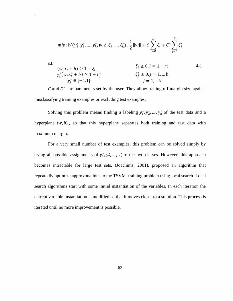
`
63
‖ ‖ ∑
∑
s.t.
4-1
(
)
are parameters set by the user. They allow trading off margin size against
misclassifying training examples or excluding test examples.
Solving this problem means finding a labeling
of the test data and a
hyperplane ⟨ ⟩ , so that this hyperplane separates both training and test data with
maximum margin.
For a very small number of test examples, this problem can be solved simply by
trying all possible assignments of
to the two classes. However, this approach
becomes intractable for large test sets. (Joachims, 2001), proposed an algorithm that
repeatedly optimize approximations to the TSVM training problem using local search. Local
search algorithms start with some initial instantiation of the variables. In each iteration the
current variable instantiation is modified so that it moves closer to a solution. This process is
iterated until no more improvement is possible.
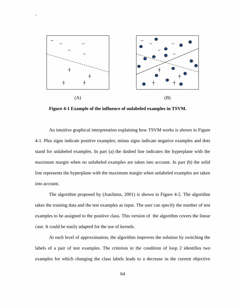
`
64
(A)
(B)
Figure 4-1 Example of the influence of unlabeled examples in TSVM.
An intuitive graphical interpretation explaining how TSVM works is shown in Figure
4-1. Plus signs indicate positive examples; minus signs indicate negative examples and dots
stand for unlabeled examples. In part (a) the dashed line indicates the hyperplane with the
maximum margin when no unlabeled examples are taken into account. In part (b) the solid
line represents the hyperplane with the maximum margin when unlabeled examples are taken
into account.
The algorithm proposed by (Joachims, 2001) is shown in Figure 4-2. The algorithm
takes the training data and the test examples as input. The user can specify the number of test
examples to be assigned to the positive class. This version of the algorithm covers the linear
case. It could be easily adapted for the use of kernels.
At each level of approximation, the algorithm improves the solution by switching the
labels of a pair of test examples. The criterion in the condition of loop 2 identifies two
examples for which changing the class labels leads to a decrease in the current objective
`
65
function. If there are no more such examples, the algorithm moves to a closer approximation
in loop 1. The function solve_svm_qp is used as a sub procedure that solves the optimization
problem 4.1, it uses the current solution as a starting point.
This algorithm is guaranteed to converge as proved by (Joachims, 2001). He also
states that the algorithm was empirically found to be robust against getting stuck in local
minima far away from the optimum.
ALGORITHM TSVM
Input: labeled examples
unlabeled examples
Output Predicted labels of the unlabeled examples
1. Train an inductive SVM M1using the labeled data .
2. Classify unlabeled documents
using M1
3. Loop1:
4. Return labels
for unlabeled documents
Figure 4-2 Algorithm for training TSV (Joachims, 1999)
While there exist unlabeled documents
1. Increase the influence of unlabeled data by incrementing
the cost factors (parameters in the algorithm)
2. Loop 2: While there exist unlabeled examples that do not
meet the restriction of the optimization problem
1. Improve the solution by switching the labels
of a pair of unlabeled examples
2. Retrain
`
66
4.2 Incorporating ontologies to TSVM
Given a collection of ontologies related to the classification problem, we build a
vector of the form:
where c is the number of classes in the classification problem. Each is a vector of
words that are known to be good discriminator for class .
Additionally, to each word could be associated a weight that corresponds to the
importance of word in discriminating its corresponding class.
For this work we focus our attention in binary classification, hence the set of classes
will be
Our proposal is to incorporate the ontologies in the algorithm, in order to use this
information to help make the decision of which unlabeled examples are worth switch to
labeled samples. We use the information of a probabilistic label given to each unlabeled
document by the ontologies. The intention is not to push too hard to conform strictly to the
ontologies, but use it as a piece of information in that point of the algorithm.
In order to use the information provided by the ontology, we first assign to each
unlabeled document a probabilistic label induced by the ontologies.
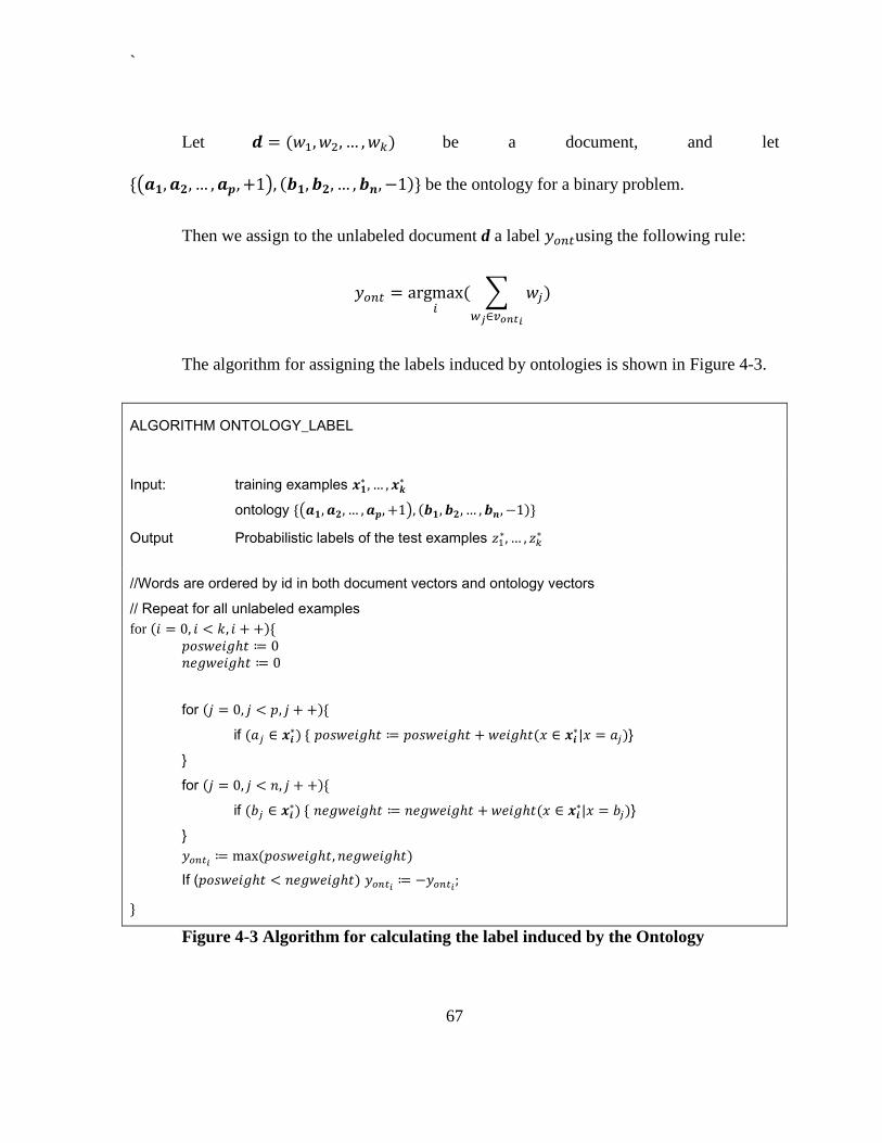
`
67
Let be a document, and let
( ) be the ontology for a binary problem.
Then we assign to the unlabeled document d a label using the following rule:
∑
The algorithm for assigning the labels induced by ontologies is shown in Figure 4-3.
ALGORITHM ONTOLOGY_LABEL
Input: training examples
ontology ( )
Output Probabilistic labels of the test examples
//Words are ordered by id in both document vectors and ontology vectors
// Repeat for all unlabeled examples
for
for
if
| }
}
for
if
| }
}
If (
Figure 4-3 Algorithm for calculating the label induced by the Ontology
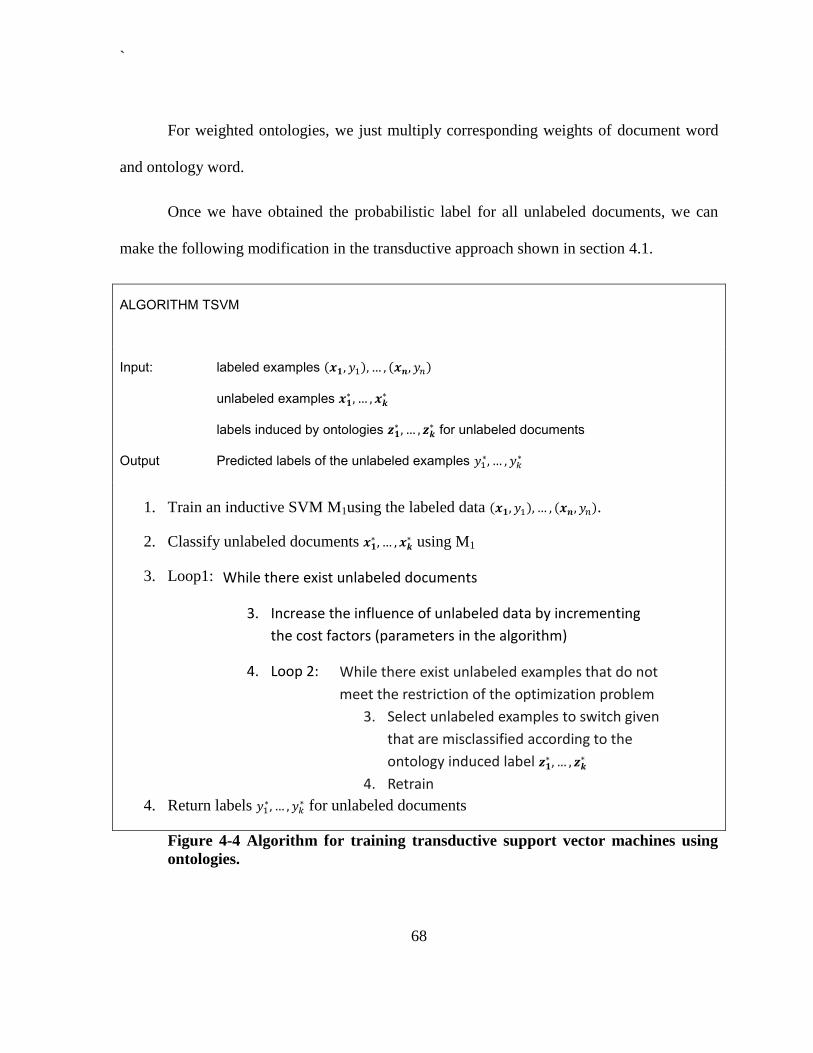
`
68
For weighted ontologies, we just multiply corresponding weights of document word
and ontology word.
Once we have obtained the probabilistic label for all unlabeled documents, we can
make the following modification in the transductive approach shown in section 4.1.
ALGORITHM TSVM
Input: labeled examples
unlabeled examples
labels induced by ontologies
for unlabeled documents
Output Predicted labels of the unlabeled examples
1. Train an inductive SVM M1using the labeled data .
2. Classify unlabeled documents
using M1
3. Loop1:
4. Return labels
for unlabeled documents
Figure 4-4 Algorithm for training transductive support vector machines using
ontologies.
While there exist unlabeled documents
3. Increase the influence of unlabeled data by incrementing
the cost factors (parameters in the algorithm)
4. Loop 2: While there exist unlabeled examples that do not
meet the restriction of the optimization problem
3. Select unlabeled examples to switch given
that are misclassified according to the
ontology induced label 𝒛𝟏 𝒛𝒌
4. Retrain
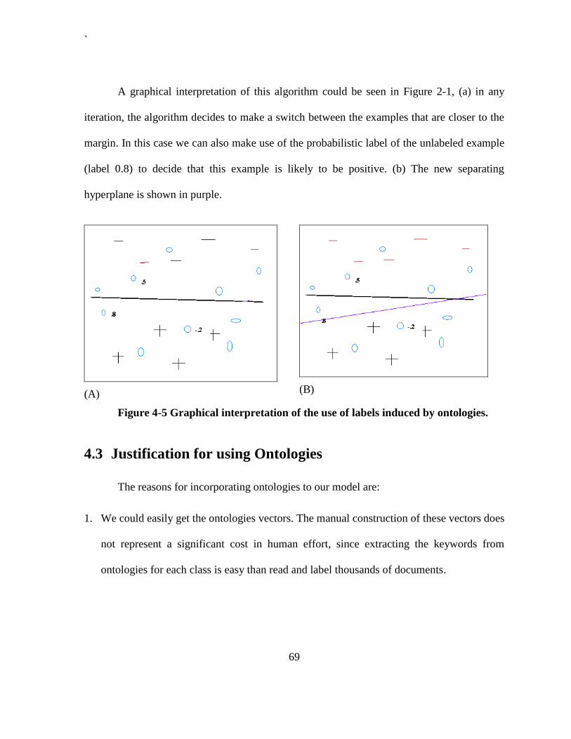
`
69
A graphical interpretation of this algorithm could be seen in Figure 2-1, (a) in any
iteration, the algorithm decides to make a switch between the examples that are closer to the
margin. In this case we can also make use of the probabilistic label of the unlabeled example
(label 0.8) to decide that this example is likely to be positive. (b) The new separating
hyperplane is shown in purple.
(A)
(B)
Figure 4-5 Graphical interpretation of the use of labels induced by ontologies.
4.3 Justification for using Ontologies
The reasons for incorporating ontologies to our model are:
1. We could easily get the ontologies vectors. The manual construction of these vectors does
not represent a significant cost in human effort, since extracting the keywords from
ontologies for each class is easy than read and label thousands of documents.
`
70
2. We can guide the classification task for the unlabeled data in a desired direction, since we
can give specific words for a class, and we can even assign weights to them. Depending
on the problem, this could be desirable.
4.4 Time Complexity of the Algorithm
Using the sparse vector representation the time complexity of the dot products depend
only on the number of non-zero entries.
Let m the maximum number of non-zero entries in any of the training examples, let q
be the rows of the Hessian. For each iteration, most time is spent on the Kernel evaluations
needed to compute the Hessian. Since we used a linear Kernel, this step has time complexity
O(q2m).
4.5 Related work
Traditionally, ontologies were used to help pre-processing text documents, such as
the use of WordNet to find synonyms to be considered as one word or token.
A distinct approach is presented in (Carlson, 2010). He extracts facts and
relationships from the web and builds ontologies. He uses these ontologies as constraints to
learn semi-supervised functions at one in a coupled manner.
Recently, (Chenthamarakshan et al., 2011) present an approach in which they first
map concepts in an ontology to the target classes of interest. They label unlabeled examples

`
71
using this mapping, in order to use them as training set for any classifier. They called this
process concept labeling.
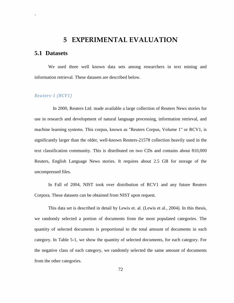
`
72
5 EXPERIMENTAL EVALUATION
5.1 Datasets
We used three well known data sets among researchers in text mining and
information retrieval. These datasets are described below.
Reuters-1 (RCV1)
In 2000, Reuters Ltd. made available a large collection of Reuters News stories for
use in research and development of natural language processing, information retrieval, and
machine learning systems. This corpus, known as "Reuters Corpus, Volume 1" or RCV1, is
significantly larger than the older, well-known Reuters-21578 collection heavily used in the
text classification community. This is distributed on two CDs and contains about 810,000
Reuters, English Language News stories. It requires about 2.5 GB for storage of the
uncompressed files.
In Fall of 2004, NIST took over distribution of RCV1 and any future Reuters
Corpora. These datasets can be obtained from NIST upon request.
This data set is described in detail by Lewis et. al. (Lewis et al., 2004). In this thesis,
we randomly selected a portion of documents from the most populated categories. The
quantity of selected documents is proportional to the total amount of documents in each
category. In Table 5-1, we show the quantity of selected documents, for each category. For
the negative class of each category, we randomly selected the same amount of documents
from the other categories.
`
73
CATEGORY LABELED UNLABELED TOTAL
Accounts/earnings 1325 25069 26394
Equity markets 1048 20296 21344
Mergers/acquisitions 960 18430 19390
Sports 813 15260 16073
Domestic politics 582 11291 11873
War, civil war 1001 17652 18653
Crime, law enforcement 466 7205 7671
Labour issues 230 6396 6626
Metals trading 505 9025 9530
Monetary/economic 533 5663 6196
Table 5-1 Number of labeled and unlabeled documents used in experiments for
10 categories of Reuters dataset.
20 Newsgroups
The 20 Newsgroups data set was collected by Ken Lang, consists of 20017 articles
divided almost evenly among 20 different UseNet discussion groups.
Some of the newsgroups are very closely related to each other (e.g.
comp.sys.ibm.pc.hardware / comp.sys.mac.hardware), while others are highly unrelated (e.g
misc.forsale / soc.religion.christian). Here is the list of the 20 newsgroups,:
comp.graphics
comp.os.ms-windows.misc
comp.sys.ibm.pc.hardware
comp.sys.mac.hardware
comp.windows.x.
rec.autos
rec.motorcycles
rec.sport.baseball
rec.sport.hockey
sci.crypt
sci.electronics
sci.med
sci.space
talk.politics.misc
talk.politics.guns
talk.politics.mideast
talk.religion.misc
alt.atheism
soc.religion.christian
misc.forsalehre
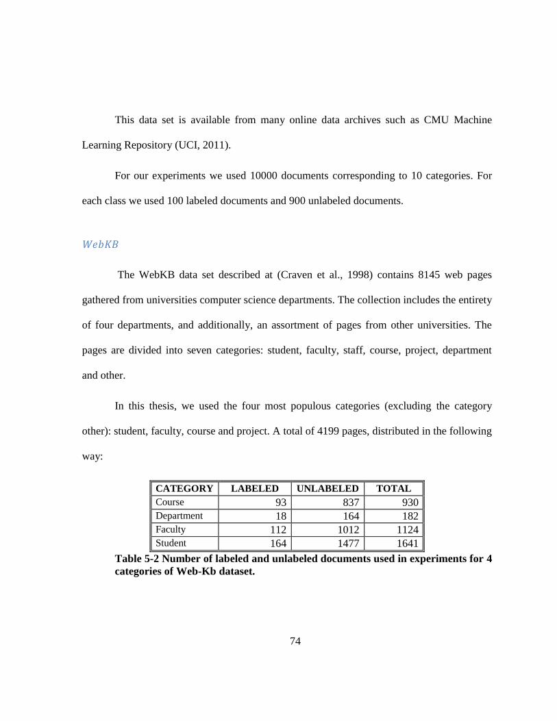
74
This data set is available from many online data archives such as CMU Machine
Learning Repository (UCI, 2011).
For our experiments we used 10000 documents corresponding to 10 categories. For
each class we used 100 labeled documents and 900 unlabeled documents.
WebKB
The WebKB data set described at (Craven et al., 1998) contains 8145 web pages
gathered from universities computer science departments. The collection includes the entirety
of four departments, and additionally, an assortment of pages from other universities. The
pages are divided into seven categories: student, faculty, staff, course, project, department
and other.
In this thesis, we used the four most populous categories (excluding the category
other): student, faculty, course and project. A total of 4199 pages, distributed in the following
way:
CATEGORY LABELED UNLABELED TOTAL
Course 93 837 930
Department 18 164 182
Faculty 112 1012 1124
Student 164 1477 1641
Table 5-2 Number of labeled and unlabeled documents used in experiments for 4
categories of Web-Kb dataset.
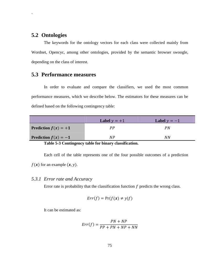
`
75
5.2 Ontologies
The keywords for the ontology vectors for each class were collected mainly from
Wordnet, Opencyc, among other ontologies, provided by the semantic browser swoogle,
depending on the class of interest.
5.3 Performance measures
In order to evaluate and compare the classifiers, we used the most common
performance measures, which we describe below. The estimators for these measures can be
defined based on the following contingency table:
Label Label
Prediction
Prediction
Table 5-3 Contingency table for binary classification.
Each cell of the table represents one of the four possible outcomes of a prediction
for an example .
5.3.1 Error rate and Accuracy
Error rate is probability that the classification function predicts the wrong class.
|
It can be estimated as:
`
76
Accuracy measures the ratio of correct predictions to the total number of cases
evaluated.
5.3.2 Asymmetric cost
In text classification problems usually negative examples exceed positive examples.
For this reason, error rate is not always a good performance measure for text classification.
Moreover, for many applications, predicting a positive example correctly is more important
than predicting a negative example correctly. For this reason this measure considers a cost
weight for the values in the contingency Table 5-3.
5.3.3 Recall
Recall is defined as the probability that a document with label is classified
correctly. It could be estimated as follows:
5.3.4 Precision
Precision is defined as the probability that a document classified as is
classified correctly. It could be estimated as follows
`
77
5.3.5 Precision / Recall breakeven point and Fβ-Measure
Precision and recall are combined to give a single measure, to make it easier to
compare learning algorithms.
Fβ-Measure is the weighted harmonic mean of precision and recall. It can be
estimated from the contingency table as:
Precision / Recall breakeven point (PRBEP) is the value at which precision and recall
are equal. is a parameter. The most commonly used value is , giving equal weight to
precision and recall.
5.4 Design Considerations
Preprocessing
We created a sparse vector representation of the documents, using normalized term
frequency.
The data sets were preprocessed to remove stop words.
Additionally, low-frequency words appearing in less than 0:2% of the documents, were
eliminated.
Implementation
Our algorithms are suited to use a sparse vector representation of documents.
Evaluation
`
78
Accuracy, Precision and Recall are used as evaluation measure.
5.5 Implementation
5.5.1 Sparse Representation
Let d the number of documents in the collection D and |V| the total number of
different words (i.e the vocabulary lenght ). In order to store the document vectors, we should
need a matrix of order O( d |V|).
However, most documents contain a small subset of the dictionary's words. In the
case of text classification, a text corpus might have thousands of word types. Each individual
document, however, has only a few hundred unique tokens. So, in the numerical vectors,
almost all of the entries for that document will be zero. Rather than store all the zeros, it is
better to represent the matrix as a set of sparse vectors, where a row is represented by a list of
pairs, one element of the pair being a column number and the other element being the
corresponding nonzero feature value. By not storing the zeros, savings in memory can be
immense. Processing programs can be adapted to handle this format.
In this thesis, we store a sparse representation of the vectors. They are stored in text
files with the form:
label ont_label w1:weight1 w2: :weight2 wk: :weightk
Each line in the text document corresponds to an document vector. Label contains the
document label for labeled documents and 0 for unlabeled documents, ont_label contains the
label obtained from the ontologies.
`
79
Then we have a sequence of pairs word id : weight. Weight is the value that
corresponds to the word for the current document. This weight could be gotten following any
of the weighting schemes sawn in section 2.2.5.
Let m be the non zero weight values of the entire collection. With this representation,
the storage growth is in the order of O(dm) which is more efficient than storing all the matrix,
since in this sparse context we have that dm <<d |V|.
We also use a sparse representation of the ontologies in the same way that the
representation used for the document vectors.
For binary classification, let p and n be the number of words extracted from
ontologies for the positive class and the negative class respectively, the vectors for the
ontologies are of the form:
+1 w1, w2, ..., wp
-1 v1, v2, ..., vn
They could also include a weight:
+1 w1:weight1, w2;weight2, ..., wp:weightp
-1 v1:weight1, v2;weight2, ..., vn:weightn
where weighti indicates a importance measure of a word wi corresponding to a class.
5.5.2 Implementation of the ontology label calculation
We use ordered list of words in order to make the algorithm efficient. In the
preprocessing step, we keep the same order in words for the ontologies than we used for the

`
80
document vectors. In a similar way than the merge part of the merge sort algorithm, we pass
through the ordered lists once.
5.5.3 Implementation of the TSVM using ontologies
We make use of a very efficient implementation of the SVM algorithm called
SVMlight
(Joachims, 1999) in order to benefit from the great characteristics that make this
algorithm computationally efficient.
The algorithm is implemented using C programming language and it has great
optimizations such as the use of working sets, shrinking of variables and caching Kernel
evaluations. The technique of caching the Kernel evaluations consists in keeping in a buffer
the calculations for the most frequent support vectors.
5.6 Experimental results
The experiments evaluate the quality and efficiency of the algorithm. The number of
documents used, and the splitting of each dataset is described in section 5.1.
For Twenty newsgroups dataset, the experiments are shown in Table 5-4, for selected
10 categories. Each category consists of 2000 examples from which 10 percent are labeled
documents. In this table we can see an improvement with respect to the TSVM in the
accuracy for three categories. The highest improvement is reached for category
soc.religion.christian. Table 5-5 shows the values of precision and recall for the same dataset. In
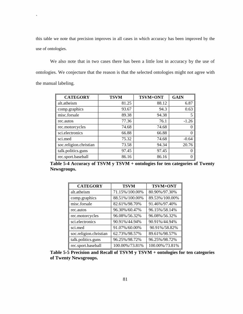
`
81
this table we note that precision improves in all cases in which accuracy has been improved by the
use of ontologies.
We also note that in two cases there has been a little lost in accuracy by the use of
ontologies. We conjecture that the reason is that the selected ontologies might not agree with
the manual labeling.
CATEGORY TSVM TSVM+ONT GAIN
alt.atheism 81.25 88.12 6.87
comp.graphics 93.67 94.3 0.63
misc.forsale 89.38 94.38 5
rec.autos 77.36 76.1 -1.26
rec.motorcycles 74.68 74.68 0
sci.electronics 66.88 66.88 0
sci.med 75.32 74.68 -0.64
soc.religion.christian 73.58 94.34 20.76
talk.politics.guns 97.45 97.45 0
rec.sport.baseball 86.16 86.16 0
Table 5-4 Accuracy of TSVM y TSVM + ontologies for ten categories of Twenty
Newsgroups.
CATEGORY TSVM TSVM+ONT
alt.atheism 71.15%/100.00% 80.90%/97.30%
comp.graphics 88.51%/100.00% 89.53%/100.00%
misc.forsale 82.61%/98.70% 91.46%/97.40%
rec.autos 96.30%/60.47% 96.15%/58.14%
rec.motorcycles 96.08%/56.32% 96.08%/56.32%
sci.electronics 90.91%/44.94% 90.91%/44.94%
sci.med 91.07%/60.00% 90.91%/58.82%
soc.religion.christian 62.73%/98.57% 89.61%/98.57%
talk.politics.guns 96.25%/98.72% 96.25%/98.72%
rec.sport.baseball 100.00%/73.81% 100.00%/73.81%
Table 5-5 Precision and Recall of TSVM y TSVM + ontologies for ten categories
of Twenty Newsgroups.
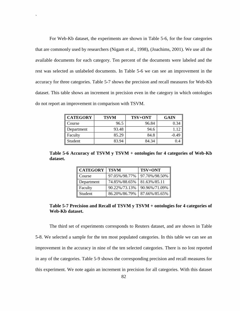
`
82
For Web-Kb dataset, the experiments are shown in Table 5-6, for the four categories
that are commonly used by researchers (Nigam et al., 1998), (Joachims, 2001). We use all the
available documents for each category. Ten percent of the documents were labeled and the
rest was selected as unlabeled documents. In Table 5-6 we can see an improvement in the
accuracy for three categories. Table 5-7 shows the precision and recall measures for Web-Kb
dataset. This table shows an increment in precision even in the category in which ontologies
do not report an improvement in comparison with TSVM.
CATEGORY TSVM TSV+ONT GAIN
Course 96.5 96.84 0.34
Department 93.48 94.6 1.12
Faculty 85.29 84.8 -0.49
Student 83.94 84.34 0.4
Table 5-6 Accuracy of TSVM y TSVM + ontologies for 4 categories of Web-Kb
dataset.
CATEGORY TSVM TSV+ONT
Course 97.05%/98.77% 97.70%/98.50%
Department 74.85%/88.65% 81.63%/85.11
Faculty 90.22%/73.13% 90.96%/71.09%
Student 86.20%/86.79% 87.66%/85.65%
Table 5-7 Precision and Recall of TSVM y TSVM + ontologies for 4 categories of
Web-Kb dataset.
The third set of experiments corresponds to Reuters dataset, and are shown in Table
5-8. We selected a sample for the ten most populated categories. In this table we can see an
improvement in the accuracy in nine of the ten selected categories. There is no lost reported
in any of the categories. Table 5-9 shows the corresponding precision and recall measures for
this experiment. We note again an increment in precision for all categories. With this dataset
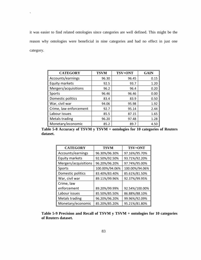
`
83
it was easier to find related ontologies since categories are well defined. This might be the
reason why ontologies were beneficial in nine categories and had no effect in just one
category.
CATEGORY TSVM TSV+ONT GAIN
Accounts/earnings 96.30 96.45 0.15
Equity markets 92.5 93.7 1.20
Mergers/acquisitions 96.2 96.4 0.20
Sports 96.46 96.46 0.00
Domestic politics 83.4 83.9 0.50
War, civil war 94.06 95.98 1.92
Crime, law enforcement 92.7 95.14 2.44
Labour issues 85.5 87.15 1.65
Metals trading 96.20 97.48 1.28
Monetary/economic 85.2 89.7 4.50
Table 5-8 Accuracy of TSVM y TSVM + ontologies for 10 categories of Reuters
dataset.
CATEGORY TSVM TSV+ONT
Accounts/earnings 96.30%/96.30% 97.16%/95.70%
Equity markets 92.50%/92.50% 93.71%/92.20%
Mergers/acquisitions 96.20%/96.20% 97.74%/95.00%
Sports 100.00%/94.06% 100.00%/94.06%
Domestic politics 83.40%/83.40% 85.61%/81.50%
War, civil war 89.11%/99.96% 92.37%/99.95%
Crime, law enforcement 89.20%/99.99% 92.54%/100.00%
Labour issues 85.50%/85.50% 86.88%/88.10%
Metals trading 96.20%/96.20% 99.96%/92.09%
Monetary/economic 85.20%/85.20% 95.21%/81.80%
Table 5-9 Precision and Recall of TSVM y TSVM + ontologies for 10 categories
of Reuters dataset.
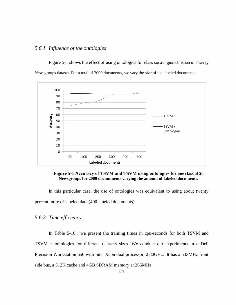
`
84
5.6.1 Influence of the ontologies
Figure 5-1 shows the effect of using ontologies for class soc.religion.christian of Twenty
Newsgroups dataset. For a total of 2000 documents, we vary the size of the labeled documents.
Figure 5-1 Accuracy of TSVM and TSVM using ontologies for one class of 20
Newsgroups for 2000 documments varying the amount of labeled documents.
In this particular case, the use of ontologies was equivalent to using about twenty
percent more of labeled data (400 labeled documents).
5.6.2 Time efficiency
In Table 5-10 , we present the training times in cpu-seconds for both TSVM and
TSVM + ontologies for different datasets sizes. We conduct our experiments in a Dell
Precision Workstation 650 with Intel Xeon dual processor, 2.80GHz. It has a 533MHz front
side bus, a 512K cache and 4GB SDRAM memory at 266MHz.
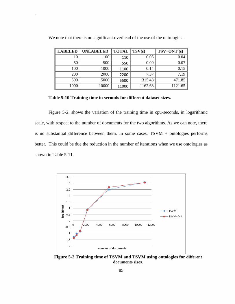
`
85
We note that there is no significant overhead of the use of the ontologies.
LABELED UNLABELED TOTAL TSV(s) TSV+ONT (s)
10 100 110 0.05 0.04
50 500 550 0.09 0.07
100 1000 1100 0.14 0.15
200 2000 2200 7.37 7.19
500 5000 5500 315.48 471.85
1000 10000 11000 1162.63 1121.65
Table 5-10 Training time in seconds for different dataset sizes.
Figure 5-2, shows the variation of the training time in cpu-seconds, in logarithmic
scale, with respect to the number of documents for the two algorithms. As we can note, there
is no substantial difference between them. In some cases, TSVM + ontologies performs
better. This could be due the reduction in the number of iterations when we use ontologies as
shown in Table 5-11.
Figure 5-2 Training time of TSVM and TSVM using ontologies for different
documents sizes.

`
86
LABELED UNLABELED TOTAL TSV(s) TSV+ONT (s)
10 100 110 0.05 0.04
50 500 550 0.09 0.07
100 1000 1100 0.14 0.15
200 2000 2200 7.37 7.19
500 5000 5500 315.48 471.85
1000 10000 11000 1162.63 1121.65
Table 5-11 Number of iterations for different dataset sizes.
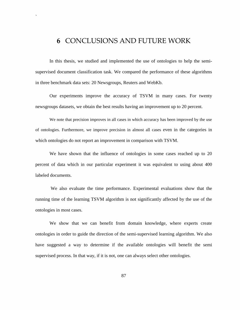
`
87
6 CONCLUSIONS AND FUTURE WORK
In this thesis, we studied and implemented the use of ontologies to help the semi-
supervised document classification task. We compared the performance of these algorithms
in three benchmark data sets: 20 Newsgroups, Reuters and WebKb.
Our experiments improve the accuracy of TSVM in many cases. For twenty
newsgroups datasets, we obtain the best results having an improvement up to 20 percent.
We note that precision improves in all cases in which accuracy has been improved by the use
of ontologies. Furthermore, we improve precision in almost all cases even in the categories in
which ontologies do not report an improvement in comparison with TSVM.
We have shown that the influence of ontologies in some cases reached up to 20
percent of data which in our particular experiment it was equivalent to using about 400
labeled documents.
We also evaluate the time performance. Experimental evaluations show that the
running time of the learning TSVM algorithm is not significantly affected by the use of the
ontologies in most cases.
We show that we can benefit from domain knowledge, where experts create
ontologies in order to guide the direction of the semi-supervised learning algorithm. We also
have suggested a way to determine if the available ontologies will benefit the semi
supervised process. In that way, if it is not, one can always select other ontologies.
`
88
Ontologies represent a new source of reliable and structured information that can be
used at different levels in the process of classifying documents, and this concept can be
extended to the use of ontologies in other areas.
Among future work that can be done based on this thesis are:
1. Include other kinds of ontologies in the process of semi-supervised learning. For example,
consider first-order logic constraints ontologies in order to incorporate the constraints to
the algorithms.
2. Identify the kernels that are well suited for document classification.
3. Design learning algorithms that work efficiently for multiclass settings, and make use of
ontologies.
4. For multiclass settings, develop a parallel algorithm in which any slave make a binary
classification.

`
89
7 ETHICAL CONSIDERATIONS
It is essential that fundamental ethical principles be applied in the design and
implementation of scientific research. The principles of research ethics have grown out of
abuses in the past. Since its formalization by the declaration of Helsinki in 1974, which
current version can be found at (WMA, 2008), in the medical field, there has been a lot of
progress. It has been proposed moral principles and practices adequate to every research area.
There is common agreement in the scientific community in principles about proper scientific
work, scientific integrity, and knowledge production practices that we will obey in this
research.
In the following, we will examine some specific ethical issues related to the main
subject of our research.
7.1 Ethics in Data Mining
Data Mining techniques allow considerable access to data. In (Fule et al., 2004) is
stated that "The process of generating rules through a mining operation becomes an ethical
issue when the results are used in decision making processes that effect people, or when
mining customer data unwittingly compromises the privacy of those customers".
In data mining research, there are a substantial number of databases that could be
considered ethically sensitive, for example in the case of medical research. The problem for
data mining researchers is that investigations using knowledge discovery tools are commonly

`
90
open ended – it is not possible to know what will be found until it is discovered. Moreover,
many useful investigations require the use of real data.
7.2 Ethics when working with documents and online information
There is a growing concern regarding the use of sensitive information stored
electronic text documents. For example, Olson (Olson, 2008) took under consideration the
ethical aspects of web mining blogs. They note that not only the privacy but, there are other
issues, for example, price discrimination. "After identifying price sensitivity by group
through data mining, the seller may offer special prices to specific customer groups" (Olson,
2008).
A main ethical concern is in the medical area, since the patient information must be
keep confidential. Suominen et. al. (Suominen et al., 2006) discuss the ethical considerations
when using text mining with nursing documentation. The principal concern is to keep
confidentiality of patients while using text mining tools.
`
91
BIBLIOGRAPHY
Alexiev, V., Breu, M., de Bruijn, J., Fensel, D., Lara, R., and Lausen, H. (2005). Information
Integration with Ontologies: Experiences from an Industrial Showcase. Wiley.
Bennett, K. a. (1992). Robust linear programming discrimination of two linearly inseparable
sets. Optimization Methods and Software 1, 23-34.
Bennett, K., and Demiriz, A. (1998). Semi-Supervised Support Vector Machines. Advances
in Neural Information Processing Systems 12, 368-374.
Berkhin, P. (2002). Survey Of Clustering Data Mining Techniques. Technical Report. Accrue
Software.
Boser, E., Guyon, M., and Vapnik, V. (1992). A training algorithm for optimal margin
classifiers. Fifth Annual Workshop on Computational Learning theory, COLT '92, (pp.
27-29). Pittsburgh, Pennsylvania, United States.
Carlson, A. (2010). Coupled Semi-Supervised Learning. Doctoral Thesis, Carnegie Mellon
University, School of Computer Science.
Chan, C., Sun, A., and Lim, E. (2001). Automated Online News Classification with
Personalization. 4th International Conference of Asian Digital Library.
Chapelle, O. S. (2008). Optimization Techniques for Semi-Supervised Support Vector
Machines. Machine Learning Research 9, 203-233.
Chenthamarakshan, V., Melville, P., Sindhwani, V., and Lawrence, R. (2011). Concept
Labeling: Building Text Classifiers with Minimal Supervision. International Joint
Conference on Artificial Intelligence (IJCAI).
Craven, M., DiPasquo, D., Freitag, D., McCallum, A., Mitchell, T., Nigam, K., et al. (1998).
Learning to extract symbolic knowledge from the World Wide Web. Fifteenth
National Conference on Artificial Intellligence.
Cristianini, N., and Shawe-Taylor, J. (2002). Support Vector Machines and other Kernel-
based Learning Methods. Cambridge University Press.
Cycorp. (2011). OpenCyc. Retrieved from OpenCyc: http://www.opencyc.org/
Fan, W., Wallace, L., Rich, S., and Zhang, Z. (2006, September). Tapping the power of text
mining. Magazine Communications of the ACM - Privacy and security in highly
dynamic systems, 49(9), pp. 77-82.
Feinerer, I. (2008). A text mining framework in R and its applications. Doctoral thesis,
University of Economics and Business, Vienna.
Feldman, R., and Sanger, J. (2007). The Text Mining Handbook. Advances Approaches in
Analyzing Unstructured Data. Cambridge.
Fule, P., and Roddick, J. (2004). Detecting privacy and ethical sensitivity in data mining
results. 27th Australasian Conference on Computer Science. Dunedin, New Zealand.
`
92
Gruber, T. (1993). A translation approach to portable ontology specifications. KNOWLEDGE
ACQUISITION, 5, 199-220.
Hearst, M. (1999). Untangling text data mining. ACL '99 Proceedings of the 37th annual
meeting of the Association for Computational Linguistics.
Hofmann, T. (1999). Probabilistic Latent Semantic Analysis. Fifteenth Conference on
Uncertainty in Artificial Intelligence .
IFOMIS. (2011). Institute for Formal Ontology and Medical Information Science. Retrieved
from Basic Formal Ontology: http://www.ifomis.org/bfo/
Jarrar, M. (2007). Towards Effectiveness and Transparency in e-Business Transactions, -An
Ontology for Customer Complaint Management. Springer.
Jenz and Partner. (n.d.). Jenz and Partner. Retrieved from The Open Source Business
Management Ontology.
Joachims, T. (1998). Text categorization with support vector machines: Learning with many
relevant features. Tenth European Conference on Machine Learning.
Joachims, T. (1999). Making large-Scale SVM Learning Practical. In B. S. Smola, Advances
in Kernel Methods - Support Vector Learning. MIT Press.
Joachims, T. (1999). Transductive inference for text classification using support vector
machines. Sixteenth International Conference of Machine Learning.
Joachims, T. (2001). Learning to classify text using support vector machines. Kluwer
Academic Publishers.
Konchady, M. (2006). Text Mining Application Programming. Charles River Media.
Krithara, A. (2008). Learning Aspect Models with Partially Labeled Data. Doctoral
Dissertation, Université Pierre et Marie Curie., , Paris.
Krithara, A., Amini, M., Renders, J., and Goutte, C. (2008). Semi-supervised Document
Classification with a Mislabeling Error Model. Advances in Information Retrieval,
30th European Conference on IR Research (ECIR'08), (pp. 370-381). Glasgow, UK.
Krithara, A., Goutte, C., Amini, M., and Renders, J. (2006). Active, Semi-Supervised
Learning for Textual Information Access. International Workshop on Intelligent
Information Access. Helsinki, Finland.
Lacy, L. (2005). Owl: Representing Information Using the Web Ontology Language.
Larocca, J., Santos, A., Kaestner, C., Neto, A., Kaestner, A., and Freitas, A. (2000).
Document Clustering and Text Summarization.
Lewis, D., Yang, Y., Rose, T., and Li, F. (2004). RCV1: A New Benchmark Collection for
Text Categorization Research. Journal of Machine Learning Research, 5, 361-397.
LOA. (2006). Laboratory of Applied Ontology. Retrieved from Descriptive Ontology for
Linguistic and Cognitive Engineering: http://www.loa.istc.cnr.it/DOLCE.html
`
93
Melville, P., Sindhwani, V., and Lawrence, R. (2009). Social media analytics: Channeling
the power of the blogosphere for marketing insight. Workshop onInformation in
Networks.
MICRA. (2011). MICRA. Retrieved from COSMO: http://micra.com/COSMO/
Mitchel, T. (2005). Generative and Discriminative Classifiers: Naive Bayes and Logistic
Regression. Retrieved from
http://www.cs.cmu.edu/~tom/mlbook/NBayesLogReg.pdf
Namburú, S., Haiying, T., L., J., and Pattipati, K. (2005). Experiments on Supervised
Learning Algorithms for Text Categorization. Aerospace Conference, 2005 IEEE.
Nigam, K. (2001). Using Unlabeled Data to Improve Text Classification. Doctoral
Dissertation, Carnegie Mellon University, School of Computer Science.
Nigam, K., McCallum, A., Thrun, S., and Mitchell, T. (1998). Learning to classify text from
labeled and unlabeled documents. Tenth Conference on Artificial intelligence.
Madison, Wisconsin, United States.
Nocedal, J., and Wright, S. (1999). Numerical Optimization. Springer.
Olson, D. (2008). Ethical aspects of web log data mining. International Journal of
Information Technology and Management, 190-200.
Pang, B., Lee, L., and Vaithyanathan, S. (2002). Thumbs up? Sentiment Classification using
Machine Learning Techniques. Conference on Empirical Methods in Natural
Language Processing (EMNLP), (pp. 79-86).
Princeton University. (2010). About WordNet. Retrieved from WordNet:
http://wordnet.princeton.edu
Sahami, M., Dumais, S., Heckerman, D., and Horvitz, E. (1998). A Bayesian Approach to
Filtering Junk E-Mail.
Shawe-Taylor, J. (2000). Support Vector Machines and other kernel-based learning methods.
Cambridge.
Suominen, H., Lehtikunnas, T., Back, B., Karsten, H., Salakoski, T., and Salanterä, S. (2006).
Theoretical considerations of ethics in text mining of nursing documents. Studies in
Health Technology and Informatics.
SWSE. (2010). SWSE. Retrieved from Semantic Web Search Engine: http://swse.deri.org/
Tong, S. (2001, November). Support Vector Machine Active Learning with Applications to
Text Classification. Journal of Machine Learning Research, 45-66.
UCI. (2011). UC Irvine Machine Learning Repository. Retrieved from Center for Machine
Learning and Intelligent Systems: http://archive.ics.uci.edu/ml/index.html
UMBC. (2007). Swoogle. Semantic Web Search. Retrieved from http://swoogle.umbc.edu/
University of Maryland. (2000). Department of Computer Science, UMD. Retrieved from
Dublin Core Ontology: http://www.cs.umd.edu/projects/plus/SHOE/onts/dublin.html
`
94
University of Washington. (2011). School of Medicine. Retrieved from Foundational Model
of Anatomy.
Weiss, S., Indurkhya, N., Zhang, T., and Damerau, F. (2004). Text Mining: Predictive
Methods for Analyzing Unstructured Information. Springer.
WMA. (2008). Declaration of Helsinki (Current Version). Retrieved from
http://www.wma.net/en/30publications/10policies/b3/
Yu, J., Ou, Y., Zhang, C., and Zhang, S. (2005). Identifying Interesting Customers through
Web Log Classification. IEEE Intelligent Systems, 20(3), 55-59.


![Semi-supervised Learning with Ladder Networkspapers.nips.cc/...semi-supervised-learning-with-ladder-networks.pdf · Semi-Supervised Learning with Ladder Networks ... 3] or classification](https://img.dokumen.tips/doc/110x75/5af9e4237f8b9ae92b8cfd03/semi-supervised-learning-with-ladder-learning-with-ladder-networks-3-or-classication.jpg)