Embed Size (px)
Citation preview

Remote Sens. 2015, 7, 13945-13974; doi:10.3390/rs71013945
remote sensing ISSN 2072-4292
www.mdpi.com/journal/remotesensing
Article
Semantic Decomposition and Reconstruction of Compound
Buildings with Symmetric Roofs from LiDAR Data and
Aerial Imagery
Hongtao Wang 1,2, Wuming Zhang 1,*, Yiming Chen 1, Mei Chen 1 and Kai Yan 1
1 State Key Laboratory of Remote Sensing Science, Beijing Key Laboratory of Environmental
Remote Sensing and Digital City, School of Geography, Beijing Normal University,
Beijing 100875, China; E-Mails: [email protected] (H.W.); [email protected] (Y.C.);
[email protected] (M.C.); [email protected] (K.Y.) 2 School of Surveying and Land Information Engineering, Henan Polytechnic University,
Jiaozuo 454003, China
* Author to whom correspondence should be addressed; E-Mail: [email protected];
Tel./Fax: +86-10-5880-9246.
Academic Editors: Norman Kerle and Prasad S. Thenkabail
Received: 11 August 2015 / Accepted: 19 October 2015 / Published: 23 October 2015
Abstract: 3D building models are important for many applications related to human
activities in urban environments. However, due to the high complexity of the building
structures, it is still difficult to automatically reconstruct building models with accurate
geometric description and semantic information. To simplify this problem, this article
proposes a novel approach to automatically decompose the compound buildings with
symmetric roofs into semantic primitives by exploiting local symmetry contained in the
building structure. In this approach, the proposed decomposition allows the overlapping of
neighbor primitives and each decomposed primitive can be represented as a parametric
form, which simplify the complexity of the building reconstruction and facilitate the
integration of LiDAR data and aerial imagery into a parameters optimization process. The
proposed method starts by extracting isolated building regions from the LiDAR point
clouds. Next, point clouds belonging to each compound building are segmented into planar
patches to construct an attributed graph, and then the local symmetries contained in the
attributed graph are exploited to automatically decompose the compound buildings into
different semantic primitives. In the final step, 2D image features are extracted depending
on the initial 3D primitives generated from LiDAR data, and then the compound building
OPEN ACCESS
Remote Sens. 2015, 7 13946
is reconstructed using constraints from LiDAR data and aerial imagery by a nonlinear least
squares optimization. The proposed method is applied to two datasets with different point
densities to show that the complexity of building reconstruction can be reduced
considerably by decomposing the compound buildings into semantic primitives. The
experimental results also demonstrate that the traditional model driven methods can be
further extended to the automated reconstruction of compound buildings by using the
proposed semantic decomposition method.
Keywords: semantic decomposition; compound building modeling; LiDAR point cloud;
aerial imagery; attributed graph
1. Introduction
3D building models are the most prominent features in digital cities and have many applications in
geographic information systems, urban planning, disaster management, emergency response, virtual
tourism, and so on. Due to the current rapid development of cities and the requirement for up-to-date
information, the automatic reconstruction of 3D building models has been an active research field in
photogrammetry and computer vision, and many approaches have been proposed on this topic based on
either photogrammetric data or LiDAR data. However, the reliable and automatic generation of detailed
large-scale building models is still a difficult and time-consuming task. In particular, the automated
generation of 3D building models with complex structures still remains a challenging issue [1,2].
Two fundamentally different methods have been used for automated 3D building reconstruction:
data-driven methods and model-driven methods. For data-driven methods, a common assumption is
that buildings have a polyhedral form, i.e., buildings only have planar roofs. Therefore, these methods
usually start with the extraction of planar patches from LiDAR point clouds using segmentation
algorithms, such as region growing [3], random sample consensus [4], 3D Hough transform [5], and
clustering methods [6,7]. Based on this segmentation, polyhedral building models are then generated
from these planar patches by intersection and step edge generation, and then some regularization rules
are often used to improve the shape of the reconstructed building model [7–9]. The main advantage of
the data-driven approach is that it can reconstruct polyhedral buildings with complex shapes. While the
main drawback of these methods is their sensitivity to the incompleteness of data arising from
occlusion, shadow and/or missing information in the input data. That is, if there are missing features in
the data, the modeling process may be hampered and the corresponding object structure may be
visually deformed. In this case, aerial imagery can serve as a complementary data source to accurately
generate building models due to its high resolution. Thus, a variety of methods using both LiDAR data
and optical imagery for building reconstruction have been proposed in the last ten years [10–19].
Among these methods, line segments, and planar patches are mainly used as the basic primitives and
the topological relationships are exploited to generate approximate building models, which are then
refined using optical images. In this process, most of the aforementioned methods need to search line
cues on multi-view aerial images, and then these 2D line segments are matched to derive the accurate
3D building structure. Although image-based edge detection algorithms perform well, matching
Remote Sens. 2015, 7 13947
ambiguities in multiple images are the main obstacle. Another limitation of the data driven methods is
that the models generated from line segments and planar patches are only geometric models, and the
semantic information about the buildings’ structures is always missed.
To obtain visual impressions and topologically-correct building models with semantic information,
geometric constraints, such as parallel and perpendicular lines should be encoded in the building
reconstruction [20,21]. Such regularization can be met easily if model driven methods are utilized. The
model-driven strategy starts with a hypothetical building model, which is then verified by the
consistency of the model with the LiDAR point clouds [22–26] or aerial imagery [27,28]. Recently, the
Reversible Jump Markov Chain Monte Carlo (RJMCMC) method has been used to generate the
building models [29,30], which performs well in the reconstruction of 3D building models. However,
its main limitation is its computational intensity. The advantage of model-driven methods is that they
can create compact, watertight, geometric building models with semantic labeling, but their main
limitation is that they can only generate certain types of predefined building models in the library, so
many existing model-driven methods usually focus on relatively simple buildings [23,27,31].
To reconstruct complex building models by using model-driven method, Constructive Solid
Geometry (CSG)-based methods have been proposed by some researchers [5,21,24,26,28,32,33].
Within these approaches, a complex building model is often regarded as a combination of simple roof
shapes, and these simple primitives are grouped into complete building models by means of Boolean
set operators (union, intersection, and subtraction). Thus, complex buildings can be reconstructed by
aggregating the basic building primitives in the library. CSG primitives have semantic information
about the model’s type and can be represented by a few shape parameters and pose parameters, which
are suitable for the building reconstruction. However, automatic decomposition of complex buildings
into CSG primitives is difficult, so the CSG modeling methods are usually adopted in a semi-automatic
way [27,34,35]. The complexity of this decomposition task has led many studies to use external
information, mostly in the form of ground plans or building footprints [5,24,25,28,32,36,37]. Among
these methods, 2D maps are used to decompose the compound buildings into non-overlapping building
regions, and then the parameters of the parametric model in each building polygon are determined
using LiDAR data or aerial imagery. The use of building footprints can simplify the reconstruction of
the complex buildings, but it is not always available and often outdated. For the automatic reconstruction
of complex buildings without ground plans, some researchers have constructed roof topology graph (a
graph indicates the topology relationship between the rooftop planar patches) to interpret the building
structures and automatically decompose complex buildings into basic primitives from LiDAR point
clouds [12,22,38–40]. By using roof topology graphs, the problem of finding basic shapes in point clouds
can be reduced to a sub-graph matching problem, and then the complex scene can be decomposed into
some predefined primitives and reconstructed by assembling these basic primitives. However, the
decomposition results of these methods are not semantic building primitives, but the combination of
planar patches or a set of polygons, which is difficult for architects to interpret and edit. In this paper, the
semantic building primitives are defined as object-based parametric building models that hold both
geometric and semantic information, which can be easily modified and reproduced.
In reality, complex buildings are often represented as compound buildings, which are the
combination of basic primitives. By decomposing the compound buildings into several semantic
primitives, the difficulty of building reconstruction can be considerably reduced. To this aim, a

Remote Sens. 2015, 7 13948
semantic decomposition method is proposed in this paper by exploiting knowledge about local
symmetries that are implicitly contained in the building structures. As a result, the compound buildings
can be decomposed into some parametric primitives (e.g., gabled roof, half-hipped roof, and hipped
roof). Then, each parametric primitive is reconstructed by a primitive-based building modeling method
proposed by Zhang et al. [41], which was developed to generate basic building primitives using
constraints from LiDAR data and aerial imagery. In contrast to the aforementioned reconstruction
methods using roof topology graph, the main contribution of this paper can be summarized as follows:
(1) automatic decomposition of compound buildings into semantic primitives by using an attributed
graph. Different from the aforementioned decomposition methods using roof topology graph, the
outputs of the proposed decomposition are semantic primitives which can be represented as fixed
parametric forms. Benefiting from this decomposition, the model driven methods can be further
extended to the automated reconstruction of the compound buildings; (2) Flexible reconstruction by
allowing the overlapping of neighbor primitives. In the process of compound building’s decomposition
and model recognition, the proposed method allows the overlapping of neighbor primitives, which can
considerably simplify the complexity of the building reconstruction because the intersection of
neighbor primitives do not need to be defined and only a small set of basic building primitives are
contained in the predefined library.
The remainder of this paper is organized as follows. The overview of the proposed method and a
detailed description of the proposed semantic decomposition and reconstruction method are given in
Section 2. In Section 3, the data sets used in this research are described, and then some experimental
results are presented. Some discussions of the proposed method are provided in Section 4. Finally,
Section 5 gives this paper’s conclusions.
2. Methodology
2.1. Overview of the Proposed Method
The proposed approach relies on the assumption that most compound buildings can be constructed as
a combination of parametric primitives, which have semantic information about the buildings’ structures
(e.g., gabled roof, half-hipped roof, hipped roof, etc.). Based on this knowledge, an automatic
decomposition algorithm is proposed to decompose the compound buildings into basic primitives, and
then each primitive is reconstructed using constraints from LiDAR data and aerial imagery.
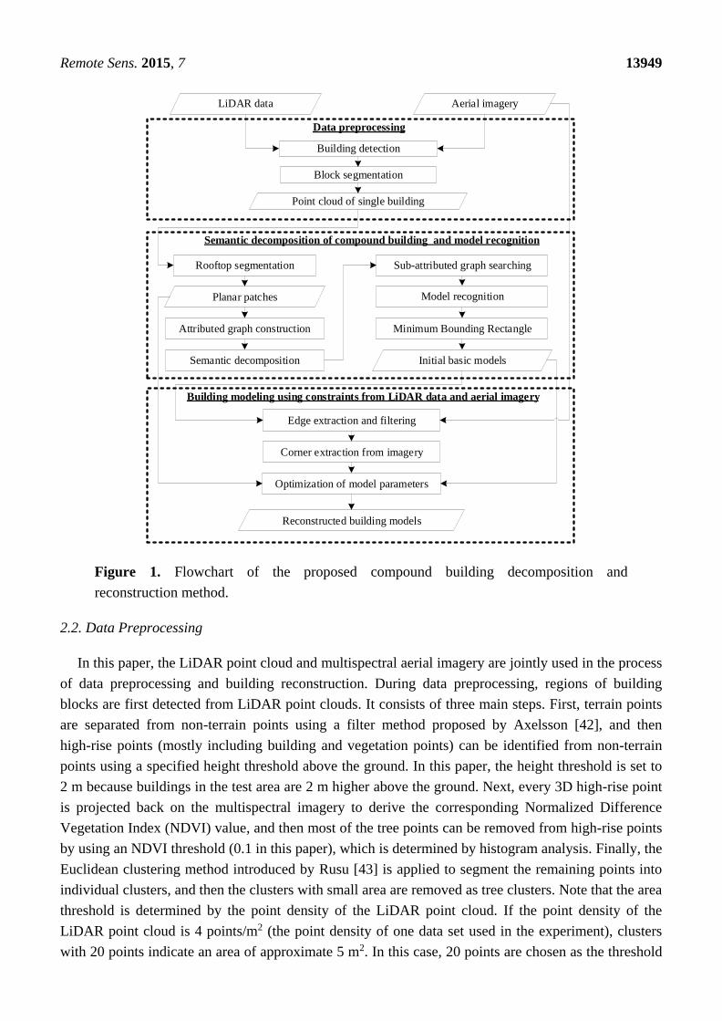
Figure 1 shows the flowchart of the proposed decomposition and reconstruction method, which
consists of three main steps. First, isolated building regions are detected and extracted from LiDAR
data during data preprocessing. In the second step, point cloud belonging to a compound building roof
is segmented into planar patches, and then an attributed graph is constructed among these segmented
planar patches. By exploiting knowledge about the local symmetries contained in the attributed graph,
the compound buildings are automatically decomposed into semantic building parts. After that, models
in each decomposition cell are recognized and estimated. In the final step, 2D corners are efficiently
extracted from the aerial imagery depending on the initial models generated from above step, and then
each primitive is reconstructed using constraints from LiDAR data and aerial imagery by a nonlinear
least squares optimization.
Remote Sens. 2015, 7 13949
LiDAR data Aerial imagery
Data preprocessing
Block segmentation
Point cloud of single building
Rooftop segmentation Sub-attributed graph searching
Planar patches
Attributed graph construction
Model recognition
Initial basic models
Optimization of model parameters
Reconstructed building models
Semantic decomposition of compound building and model recognition
Building modeling using constraints from LiDAR data and aerial imagery
Building detection
Semantic decomposition
Minimum Bounding Rectangle
Edge extraction and filtering
Corner extraction from imagery
Figure 1. Flowchart of the proposed compound building decomposition and
reconstruction method.
2.2. Data Preprocessing
In this paper, the LiDAR point cloud and multispectral aerial imagery are jointly used in the process
of data preprocessing and building reconstruction. During data preprocessing, regions of building
blocks are first detected from LiDAR point clouds. It consists of three main steps. First, terrain points
are separated from non-terrain points using a filter method proposed by Axelsson [42], and then
high-rise points (mostly including building and vegetation points) can be identified from non-terrain
points using a specified height threshold above the ground. In this paper, the height threshold is set to
2 m because buildings in the test area are 2 m higher above the ground. Next, every 3D high-rise point
is projected back on the multispectral imagery to derive the corresponding Normalized Difference
Vegetation Index (NDVI) value, and then most of the tree points can be removed from high-rise points
by using an NDVI threshold (0.1 in this paper), which is determined by histogram analysis. Finally, the
Euclidean clustering method introduced by Rusu [43] is applied to segment the remaining points into
individual clusters, and then the clusters with small area are removed as tree clusters. Note that the area
threshold is determined by the point density of the LiDAR point cloud. If the point density of the
LiDAR point cloud is 4 points/m2 (the point density of one data set used in the experiment), clusters
with 20 points indicate an area of approximate 5 m2. In this case, 20 points are chosen as the threshold
Remote Sens. 2015, 7 13950
to remove tree clusters smaller than 5 m2. After the aforementioned process, building points will be
detected and segmented into clusters that represent the individual buildings, and then building models
can be subsequently reconstructed from each collection.
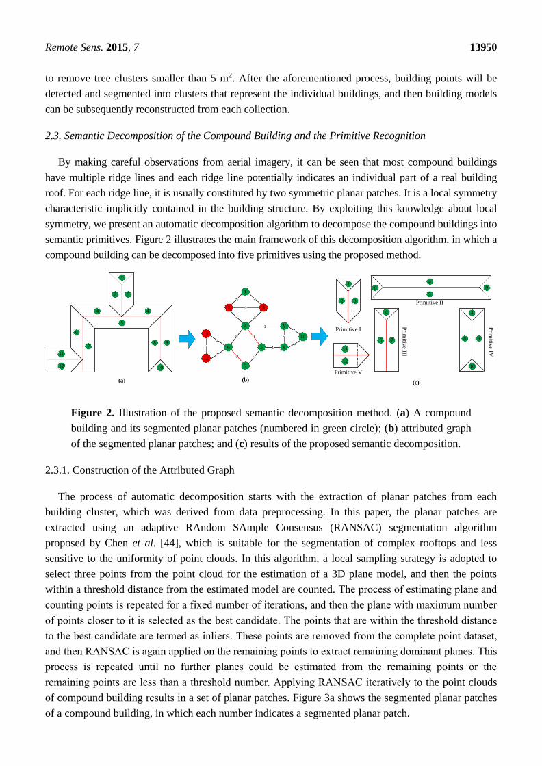
2.3. Semantic Decomposition of the Compound Building and the Primitive Recognition
By making careful observations from aerial imagery, it can be seen that most compound buildings
have multiple ridge lines and each ridge line potentially indicates an individual part of a real building
roof. For each ridge line, it is usually constituted by two symmetric planar patches. It is a local symmetry
characteristic implicitly contained in the building structure. By exploiting this knowledge about local
symmetry, we present an automatic decomposition algorithm to decompose the compound buildings into
semantic primitives. Figure 2 illustrates the main framework of this decomposition algorithm, in which a
compound building can be decomposed into five primitives using the proposed method.
1
2 3
4 4
5
6
78 9
1
2 3
4
6
7
10
5 8
9
12
2
10
11
11
12
2
22
2
1 1
1 1
1
1
1
1
1
1
1
1
1
2 3
4
5
11
12
Primitive I
Primitive V
Primitive II
(a) (b)
6 7 8 9
10
Prim
itive IV
Prim
itive III
4 4
(c)
6 9
Figure 2. Illustration of the proposed semantic decomposition method. (a) A compound
building and its segmented planar patches (numbered in green circle); (b) attributed graph
of the segmented planar patches; and (c) results of the proposed semantic decomposition.
2.3.1. Construction of the Attributed Graph
The process of automatic decomposition starts with the extraction of planar patches from each
building cluster, which was derived from data preprocessing. In this paper, the planar patches are
extracted using an adaptive RAndom SAmple Consensus (RANSAC) segmentation algorithm
proposed by Chen et al. [44], which is suitable for the segmentation of complex rooftops and less
sensitive to the uniformity of point clouds. In this algorithm, a local sampling strategy is adopted to
select three points from the point cloud for the estimation of a 3D plane model, and then the points
within a threshold distance from the estimated model are counted. The process of estimating plane and
counting points is repeated for a fixed number of iterations, and then the plane with maximum number
of points closer to it is selected as the best candidate. The points that are within the threshold distance
to the best candidate are termed as inliers. These points are removed from the complete point dataset,
and then RANSAC is again applied on the remaining points to extract remaining dominant planes. This
process is repeated until no further planes could be estimated from the remaining points or the
remaining points are less than a threshold number. Applying RANSAC iteratively to the point clouds
of compound building results in a set of planar patches. Figure 3a shows the segmented planar patches
of a compound building, in which each number indicates a segmented planar patch.

Remote Sens. 2015, 7 13951
1
2 3
4 4
5
6
78 9
1
2 3
4
6
7
10
5 8
9
12
10
11
11
12
(a) (b)
1
2 3
4
6
7
10
5 8
9
12
2
112
22
2
1 1
1 1
1
1
1
1
1
1
1
1
(c)
1
2 3
4
6
7
10
5 8
9
12
2
11
2
22
2
1 1
1 1
1
1
1
1
1
1
1
1
(d)
1
2 3
4
6
7
10
5 8
9
12
2
11
2
22
2
1 1
1 1
1
1
1
1
1
1
1
1
(e)
1
2 3
4
6
7
10
5 8
9
12
2
11
2
22
2
1 1
1 1
1
1
1
1
1
1
1
1
(f)
Figure 3. The construction of a compound building’s attributed graph. (a) The segmented
planar patches of a compound building; (b) adjacency graph of the segmented planar
patches; (c) edge labeling according to the normal vector of two adjacent planar patches;
(d) extraction of anti-symmetry planar patches; (e) grouping of remaining planar patches;
and (f) attributed graph of a compound building.
To decompose the compound buildings into semantic primitives, an adjacency graph is first
constructed using the segmented planar segments to encode the building topology. In this graph, each
vertex represents a planar patch in the building structure, and an edge between two vertices indicates
that the two planar patches are spatially connected. In this study, the adjacency relationships of all
pairs of roof planar patches are reconstructed using the boundary points of each planar patch to reduce
the complexity of calculation. More specifically, the boundary points of each planar segment are first
detected using the alpha shape algorithm [45], and then the distances between two boundary point sets
of the planar patches are calculated. The vertices representing two planar patches are connected if two
constraints are satisfied: (1) the distance between the boundary point sets of the two planar patches is
less than a predefined threshold; and (2) there are sufficient number of corresponding point pairs that
satisfy the first constraint. Applying these two criteria, the adjacency relationships of all the pairs of
segmented roof planar patches can be determined and used to decompose the compound buildings.
Figure 3b shows the adjacency graph of the segmented planar patches shown in Figure 3a.
However, representation solely based on adjacency graphs is not sufficient to discriminate different
semantic primitives. To make the decomposition more reliable, another topological relationship is
embedded into the adjacency graph, which is the normal direction of each planar segment.
Specifically, the topological relationship between two adjacent planar patches can be described by
considering the proximity and normal vector of two planar patches. In this paper, the equation of a 3D
plane is defined as AX + BY + CZ + D = 0. In this case, the normal vector of a 3D plane is the plane
parameters (A, B, C), which can be estimated by a number of 3D points located on the same planar
Remote Sens. 2015, 7 13952
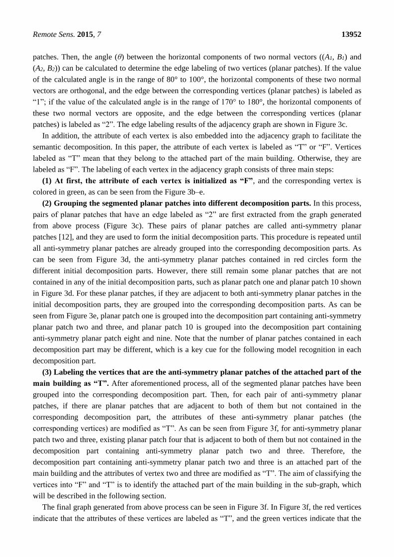
patches. Then, the angle (θ) between the horizontal components of two normal vectors ((A1, B1) and
(A2, B2)) can be calculated to determine the edge labeling of two vertices (planar patches). If the value
of the calculated angle is in the range of 80° to 100°, the horizontal components of these two normal
vectors are orthogonal, and the edge between the corresponding vertices (planar patches) is labeled as
“1”; if the value of the calculated angle is in the range of 170° to 180°, the horizontal components of
these two normal vectors are opposite, and the edge between the corresponding vertices (planar
patches) is labeled as “2”. The edge labeling results of the adjacency graph are shown in Figure 3c.
In addition, the attribute of each vertex is also embedded into the adjacency graph to facilitate the
semantic decomposition. In this paper, the attribute of each vertex is labeled as “T” or “F”. Vertices
labeled as “T” mean that they belong to the attached part of the main building. Otherwise, they are
labeled as “F”. The labeling of each vertex in the adjacency graph consists of three main steps:
(1) At first, the attribute of each vertex is initialized as “F”, and the corresponding vertex is
colored in green, as can be seen from the Figure 3b–e.
(2) Grouping the segmented planar patches into different decomposition parts. In this process,
pairs of planar patches that have an edge labeled as “2” are first extracted from the graph generated
from above process (Figure 3c). These pairs of planar patches are called anti-symmetry planar
patches [12], and they are used to form the initial decomposition parts. This procedure is repeated until
all anti-symmetry planar patches are already grouped into the corresponding decomposition parts. As
can be seen from Figure 3d, the anti-symmetry planar patches contained in red circles form the
different initial decomposition parts. However, there still remain some planar patches that are not
contained in any of the initial decomposition parts, such as planar patch one and planar patch 10 shown
in Figure 3d. For these planar patches, if they are adjacent to both anti-symmetry planar patches in the
initial decomposition parts, they are grouped into the corresponding decomposition parts. As can be
seen from Figure 3e, planar patch one is grouped into the decomposition part containing anti-symmetry
planar patch two and three, and planar patch 10 is grouped into the decomposition part containing
anti-symmetry planar patch eight and nine. Note that the number of planar patches contained in each
decomposition part may be different, which is a key cue for the following model recognition in each
decomposition part.
(3) Labeling the vertices that are the anti-symmetry planar patches of the attached part of the
main building as “T”. After aforementioned process, all of the segmented planar patches have been
grouped into the corresponding decomposition part. Then, for each pair of anti-symmetry planar
patches, if there are planar patches that are adjacent to both of them but not contained in the
corresponding decomposition part, the attributes of these anti-symmetry planar patches (the
corresponding vertices) are modified as “T”. As can be seen from Figure 3f, for anti-symmetry planar
patch two and three, existing planar patch four that is adjacent to both of them but not contained in the
decomposition part containing anti-symmetry planar patch two and three. Therefore, the
decomposition part containing anti-symmetry planar patch two and three is an attached part of the
main building and the attributes of vertex two and three are modified as “T”. The aim of classifying the
vertices into “F” and “T” is to identify the attached part of the main building in the sub-graph, which
will be described in the following section.
The final graph generated from above process can be seen in Figure 3f. In Figure 3f, the red vertices
indicate that the attributes of these vertices are labeled as “T”, and the green vertices indicate that the
Remote Sens. 2015, 7 13953
attribute of these vertices are labeled as “F”. Such graph is called an attributed graph, which can be
used to find the plausible decomposition of compound buildings.
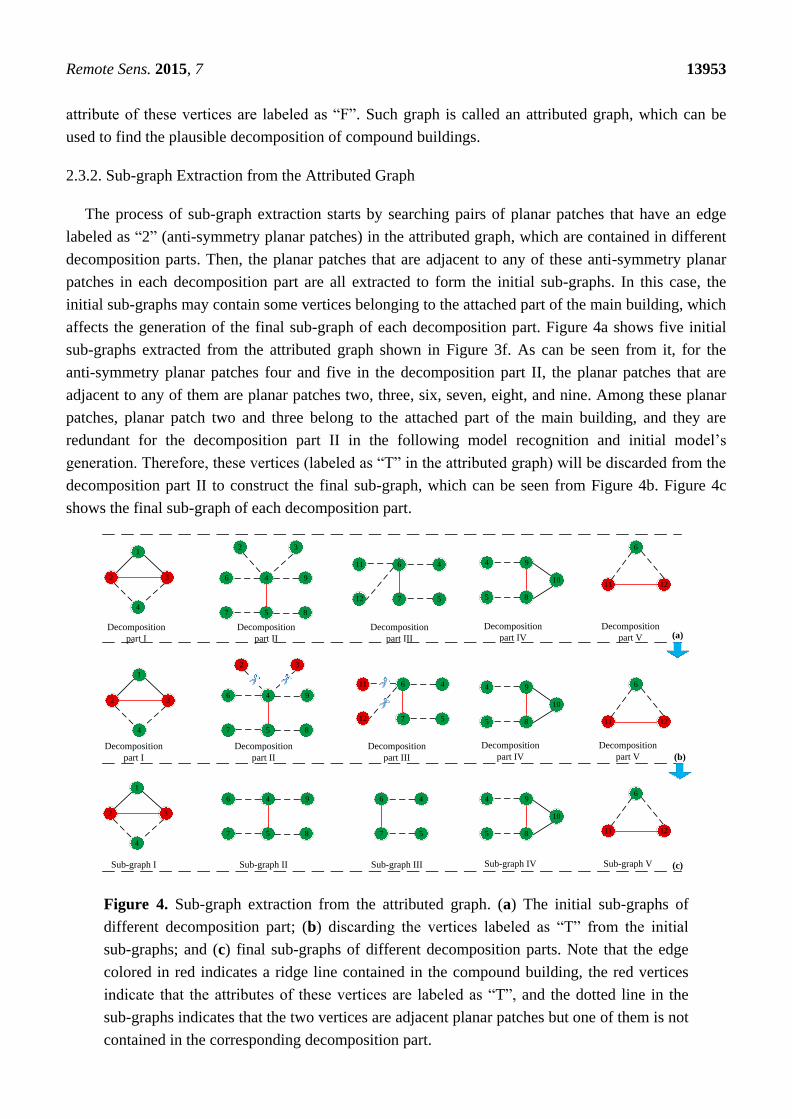
2.3.2. Sub-graph Extraction from the Attributed Graph
The process of sub-graph extraction starts by searching pairs of planar patches that have an edge
labeled as “2” (anti-symmetry planar patches) in the attributed graph, which are contained in different
decomposition parts. Then, the planar patches that are adjacent to any of these anti-symmetry planar
patches in each decomposition part are all extracted to form the initial sub-graphs. In this case, the
initial sub-graphs may contain some vertices belonging to the attached part of the main building, which
affects the generation of the final sub-graph of each decomposition part. Figure 4a shows five initial
sub-graphs extracted from the attributed graph shown in Figure 3f. As can be seen from it, for the
anti-symmetry planar patches four and five in the decomposition part II, the planar patches that are
adjacent to any of them are planar patches two, three, six, seven, eight, and nine. Among these planar
patches, planar patch two and three belong to the attached part of the main building, and they are
redundant for the decomposition part II in the following model recognition and initial model’s
generation. Therefore, these vertices (labeled as “T” in the attributed graph) will be discarded from the
decomposition part II to construct the final sub-graph, which can be seen from Figure 4b. Figure 4c
shows the final sub-graph of each decomposition part.
7
10
58
96 4
4
58
9
7 5
6 4
1
2 3
4
7
10
5 8
96 4 4
58
9
7 5
6 4
2 3
12
11
1
2 3
47
10
5
8
9
6 4
4
5
8
9
7 5
6 4
2 3
12
11
11 12
6
1
2 3
411 12
6
11 12
6
(a)
(b)
(c)
Decomposition
part I
Decomposition
part II
Decomposition
part III
Decomposition
part IV
Decomposition
part V
Decomposition
part I
Decomposition
part II
Decomposition
part III
Decomposition
part IV
Decomposition
part V
Sub-graph I Sub-graph II Sub-graph III Sub-graph IV Sub-graph V
Figure 4. Sub-graph extraction from the attributed graph. (a) The initial sub-graphs of
different decomposition part; (b) discarding the vertices labeled as “T” from the initial
sub-graphs; and (c) final sub-graphs of different decomposition parts. Note that the edge
colored in red indicates a ridge line contained in the compound building, the red vertices
indicate that the attributes of these vertices are labeled as “T”, and the dotted line in the
sub-graphs indicates that the two vertices are adjacent planar patches but one of them is not
contained in the corresponding decomposition part.
Remote Sens. 2015, 7 13954
Note that if the vertices labeled as “T” are the anti-symmetry planar patches in the corresponding
decomposition part, they will not be discarded from the initial sub-graph. As can be seen from Figure 4a,
planar patch two and three are the anti-symmetry planar patches of the decomposition part I, but not
the anti-symmetry planar patches of the decomposition part II (planar patch four and five are the
anti-symmetry planar patches of the decomposition part II). Therefore, though the vertex two and three
are labeled as “T”, they are reserved in the sub-graph I but discarded from the sub-graph II.
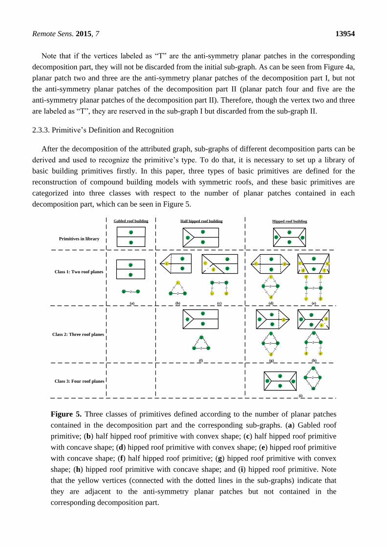
2.3.3. Primitive’s Definition and Recognition
After the decomposition of the attributed graph, sub-graphs of different decomposition parts can be
derived and used to recognize the primitive’s type. To do that, it is necessary to set up a library of
basic building primitives firstly. In this paper, three types of basic primitives are defined for the
reconstruction of compound building models with symmetric roofs, and these basic primitives are
categorized into three classes with respect to the number of planar patches contained in each
decomposition part, which can be seen in Figure 5.
Class 1: Two roof planes
Class 2: Three roof planes
Class 3: Four roof planes
Primitives in library
a b2
a b2
c
d
1
1
1
1
a
b
a
b
a
b
c
a
b
c
a
b
c d
a b2
c
1 1
a b2
c
1
1
1
1
a b2
c
d
1
1
1
1
a b2
c
1 1
d
a
b
c
a
b
a b2
1
1
c d
a b2
1
1
c d
e f
1
1
a b2
c
1
1
1
1
d e
Gabled roof building Half hipped roof building Hipped roof building
a
b
a
b
c
d
c
d
e
c d c e
d f
d
(a)
(f)
(c)(b)
(i)
(d) (e)
(g) (h)
a
b
a
b
c
a
b
c d
Figure 5. Three classes of primitives defined according to the number of planar patches
contained in the decomposition part and the corresponding sub-graphs. (a) Gabled roof
primitive; (b) half hipped roof primitive with convex shape; (c) half hipped roof primitive
with concave shape; (d) hipped roof primitive with convex shape; (e) hipped roof primitive
with concave shape; (f) half hipped roof primitive; (g) hipped roof primitive with convex
shape; (h) hipped roof primitive with concave shape; and (i) hipped roof primitive. Note
that the yellow vertices (connected with the dotted lines in the sub-graphs) indicate that
they are adjacent to the anti-symmetry planar patches but not contained in the
corresponding decomposition part.
Remote Sens. 2015, 7 13955
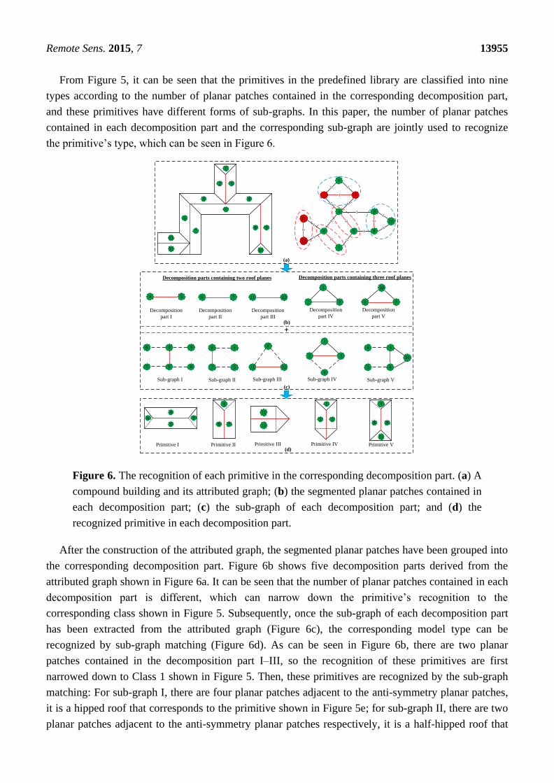
From Figure 5, it can be seen that the primitives in the predefined library are classified into nine
types according to the number of planar patches contained in the corresponding decomposition part,
and these primitives have different forms of sub-graphs. In this paper, the number of planar patches
contained in each decomposition part and the corresponding sub-graph are jointly used to recognize
the primitive’s type, which can be seen in Figure 6.
1
2 3
4
6
7
10
5 8
9
12
2
112
22
2
1 1
1 1
1
1
1
1
1
1
1
1
1
2 3
4 5 6 78 9
10
11 12
1
2 3
4
7
10
5 8
96 4 4
58
9
7 5
6 4
11 12
6
Decomposition parts containing two roof planes Decomposition parts containing three roof planes
1
2 3
4
5
6 9
6 7 8 9
10
11
12
Primitive III Primitive VPrimitive IIPrimitive I Primitive IV
44
1
2 3
4 4
5
6
78 9
10
11
12
Sub-graph I Sub-graph III Sub-graph VSub-graph II Sub-graph IV
Decomposition
part I
Decomposition
part II
Decomposition
part III
Decomposition
part IV
Decomposition
part V
+
(a)
(b)
(c)
(d)
Figure 6. The recognition of each primitive in the corresponding decomposition part. (a) A
compound building and its attributed graph; (b) the segmented planar patches contained in
each decomposition part; (c) the sub-graph of each decomposition part; and (d) the
recognized primitive in each decomposition part.
After the construction of the attributed graph, the segmented planar patches have been grouped into
the corresponding decomposition part. Figure 6b shows five decomposition parts derived from the
attributed graph shown in Figure 6a. It can be seen that the number of planar patches contained in each
decomposition part is different, which can narrow down the primitive’s recognition to the
corresponding class shown in Figure 5. Subsequently, once the sub-graph of each decomposition part
has been extracted from the attributed graph (Figure 6c), the corresponding model type can be
recognized by sub-graph matching (Figure 6d). As can be seen in Figure 6b, there are two planar
patches contained in the decomposition part I–III, so the recognition of these primitives are first
narrowed down to Class 1 shown in Figure 5. Then, these primitives are recognized by the sub-graph
matching: For sub-graph I, there are four planar patches adjacent to the anti-symmetry planar patches,
it is a hipped roof that corresponds to the primitive shown in Figure 5e; for sub-graph II, there are two
planar patches adjacent to the anti-symmetry planar patches respectively, it is a half-hipped roof that
Remote Sens. 2015, 7 13956
corresponds to the primitive shown in Figure 5c; for sub-graph III, there is only one planar patch
adjacent to both anti-symmetry planar patches, it is a variant of half hipped roof building that
corresponds to the primitive shown in Figure 5b. The aforementioned recognition method can also be
applied to the decomposition part containing three roof planes. For example, there are two planar
patches adjacent to both anti-symmetry planar patches in sub-graph IV, it is a variant of hipped roof
that corresponds to the primitive shown in Figure 5g.
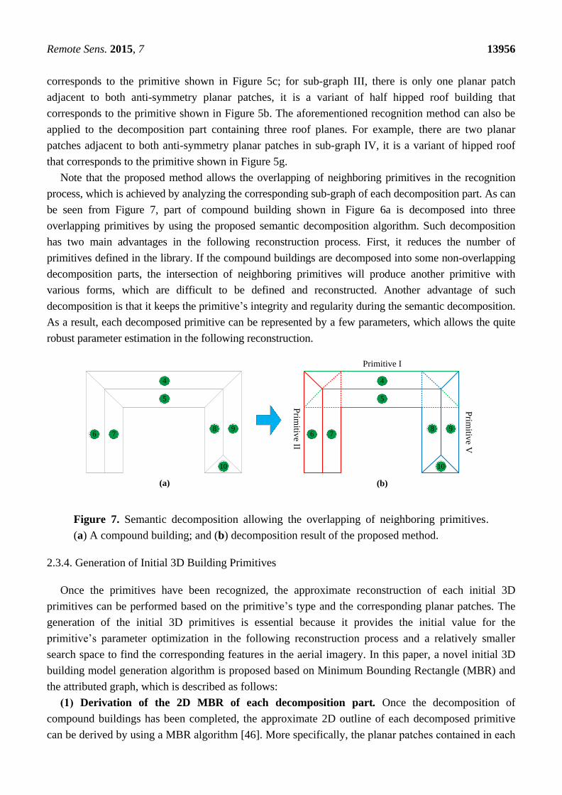
Note that the proposed method allows the overlapping of neighboring primitives in the recognition
process, which is achieved by analyzing the corresponding sub-graph of each decomposition part. As can
be seen from Figure 7, part of compound building shown in Figure 6a is decomposed into three
overlapping primitives by using the proposed semantic decomposition algorithm. Such decomposition
has two main advantages in the following reconstruction process. First, it reduces the number of
primitives defined in the library. If the compound buildings are decomposed into some non-overlapping
decomposition parts, the intersection of neighboring primitives will produce another primitive with
various forms, which are difficult to be defined and reconstructed. Another advantage of such
decomposition is that it keeps the primitive’s integrity and regularity during the semantic decomposition.
As a result, each decomposed primitive can be represented by a few parameters, which allows the quite
robust parameter estimation in the following reconstruction.
4
5
6 78 9
10
Primitive I
(a)
Prim
itive V
Prim
itive II
4
5
6 78 9
10
(b)
Figure 7. Semantic decomposition allowing the overlapping of neighboring primitives.
(a) A compound building; and (b) decomposition result of the proposed method.
2.3.4. Generation of Initial 3D Building Primitives
Once the primitives have been recognized, the approximate reconstruction of each initial 3D
primitives can be performed based on the primitive’s type and the corresponding planar patches. The
generation of the initial 3D primitives is essential because it provides the initial value for the
primitive’s parameter optimization in the following reconstruction process and a relatively smaller
search space to find the corresponding features in the aerial imagery. In this paper, a novel initial 3D
building model generation algorithm is proposed based on Minimum Bounding Rectangle (MBR) and
the attributed graph, which is described as follows:
(1) Derivation of the 2D MBR of each decomposition part. Once the decomposition of
compound buildings has been completed, the approximate 2D outline of each decomposed primitive
can be derived by using a MBR algorithm [46]. More specifically, the planar patches contained in each

Remote Sens. 2015, 7 13957
decomposition part are projected onto the XY plane to derive the convex hull, and then the 2D MBR is
determined by the rectangle with minimum area that contains all the 2D convex hull points. The MBRs
of two decomposed primitives can be seen in Figure 8, which are colored in yellow. The utility of the
2D MBR is that it can provide the approximate 2D eave corners (corners (1–4) in Figure 8) of each
decomposed primitive, which is crucial for the generation of initial 3D primitives. In addition, the 2D
MBR can be used to determine the initial parameters and the main orientation of each decomposed
primitive, which is necessary for the subsequent reconstruction steps.
a b
e
d
d d
a b
e
c c
MBR MBR
(1)
(2) (4)
(3)
(5)
(6)
(1)
(2) (4)
(3)
(5)
(6)
(a) (b)
Figure 8. The generation of initial 3D primitives using MBRs and the corresponding
planar patches. (a) The generation of initial 3D primitives with concave shapes; and (b) the
generation of initial 3D primitives with convex shapes.
(2) Generation of the initial 3D primitives. To derive the initial 3D primitives, the approximate 3D
corners of each primitive should be calculated. In this study, 3D corners of primitives are classified as
eave corners (corners (1–4) in Figure 8) and ridge corners (corners (5–6) in Figure 8) because they are
calculated by using different methods. For ridge corners, they are calculated by the intersection of
concurrent planar patches. For example, 3D coordinates of the corner (5) in Figure 8 can be calculated by
the intersection of planar patch a, b, and c. However, the 3D eave corners cannot be calculated by the
intersection of 3D planes because the wall planes are absent. In this case, the 2D MBRs can substitute the
walls to provide the approximate 2D eave corners (xi, yi) of each decomposed primitive, and then the 3D
eave corners can be calculated by using the 2D eave corners and the corresponding 3D plane equation.
As can be seen from Figure 8a, 3D coordinates of the eave corners (1–2) can be calculated by using the
2D eave corners ((x1, y1), (x2, y2)) and the 3D plane equation of planar patch a.
However, the 3D eave corners of basic primitives with convex shapes may not be located at the
corners of the MBR, which can be seen in Figure 8b. In this case, corner (2) and corner (4) cannot be
calculated using the MBR and the corresponding 3D planes. To address this problem, a 3D plane
(bottom plane) is first estimated using the 3D coordinates calculated from the MBR and anti-symmetry
planar patches, and then the 3D eave corner can be derived using this bottom plane and two adjacent
planes. For example, 3D eave corner (2) in Figure 8b can be derived by the intersection of planar patch
a, d and the estimated bottom plane. Note that the primitive’s type determines the calculation method
of the 3D eave corners. For example, the 3D eave corners of primitive (b), (d), and (g) in Figure 5 are
Remote Sens. 2015, 7 13958
calculated by using the method illustrated in Figure 8b, and the 3D eave corners of other primitives are
calculated by using the method illustrated in Figure 8a.
2.4. Image Feature Extraction and Building Modeling
The main idea of the proposed method is to decompose compound buildings into basic building
primitives, and then each building primitive is reconstructed using the constraints from LiDAR data
and aerial imagery. In this process, the relevant features should first be extracted from the LiDAR data
and aerial imagery to form the cost function, and then a non-linear least squares optimization is
performed to reconstruct the building model. In this study, the features from LiDAR data are the
segmented planar patches which have been extracted by RANSAC, and the features from the
perspective aerial imagery are the 2D image corners of each building primitive which can be derived
depending on the initial 3D building primitives generated from above process.
2.4.1. Feature Extraction from Perspective Aerial Imagery
Using the known orientation parameters of the aerial imagery, the initial building primitives derived
from LiDAR data can be projected onto the corresponding aerial imagery, which can be seen in
Figure 9a. It can be seen that, the back projected wireframe provides a relatively smaller searching
space to find the corresponding features in the aerial imagery. Thus, a buffer is constructed from the
initial building’s boundary to derive a sub-image, and then the corner extraction procedure is
conducted on this sub-image as follows:
(1) The discrete edge pixels are first detected by applying a canny edge detector [47] on the
sub-image where the initial building primitive appears, followed by linking edge pixels to derive line
segments. Then, line segments whose lengths are smaller than a given threshold are removed. The
resulting edge map is shown in Figure 9b. It can be observed that there are still too many edge pixels in
the building region and it is hard to find the correct building edges.
(2) To filter the irrelevant edge pixels, buffer regions are generated based on each back projected
edge of the initial model (pairs of red dot lines in Figure 9c), and only the edge pixels that are inside
the defined buffer are considered as candidate edge pixels. The buffer size is set according to the point
spacing of the LiDAR point cloud. Figure 9c shows the edge pixels located in each buffer region of an
initial hipped roof model; different colors represent different groups of edge pixels in the buffer zone.
(3) As seen in Figure 9c, there are many edge pixels that do not belong to the actual building
boundaries still reserved in each buffer, so the RANSAC algorithm [48] is applied to each group of
edge pixels to filter irrelevant edge pixels again, and then the inliers can be used to estimate the
equations of 2D straight lines. The result can be seen in Figure 9d; pixels with different colors indicate
different groups of inliers.
(4) During back projection, the geometry and topology of the initial building primitives are
transformed into two dimensional features, and the topological relationships between them are
preserved. That is, once the primitive’s type is determined, the relationships among the corners and the
corresponding model edges are available from a 3D initial model reconstructed from LiDAR data.
Consequently, after the straight lines have been derived from the aforementioned steps, the 2D corners

Remote Sens. 2015, 7 13959
of each building primitive can be extracted by the intersection of neighboring straight lines, which can
be seen in Figure 9e.
Figure 9. The process of corner extraction from aerial imagery. (a) Initial model back
projected onto the corresponding aerial imagery; (b) initial model superimposed onto the
edge map; (c) edge pixels in the buffer zone; (d) inliers of RANSAC superimposed onto
the gray image; and (e) the extracted 2D corners.
2.4.2. Building Modeling Using Constraints from LiDAR Data and Perspective Aerial Imagery
After the aforementioned process, both the planar patches and the accurate 2D image corner of each
building primitive can be acquired, together with the primitive’s type and initial parameters, the
accurate 3D building primitives can be derived by using a primitive-based reconstruction algorithm
proposed by Zhang et al [41]. In this method, two constraints from LiDAR data and aerial imagery are
used for the reconstruction of each building primitive. First, the back-projections of the 3D primitive’s
vertices onto the aerial image should perfectly superpose onto the extracted corners; this constraint can
be expressed by the collinearity equation. Second, the primitive’s vertices should be exactly on the 3D
planes extracted from LiDAR point clouds; this constraint can be expressed by the point-to-plane
distance. According to these constraints, the observation functions can be established as Equation (1).
𝑥𝑖 = 𝑥𝑝 − 𝑓𝑎1(𝑋𝑖 − 𝑋𝑆) + 𝑏1(𝑌𝑖 − 𝑌𝑆) + 𝑐1(𝑍𝑖 − 𝑍𝑆)
𝑎3(𝑋𝑖 − 𝑋𝑆) + 𝑏3(𝑌𝑖 − 𝑌𝑆) + 𝑐3(𝑍𝑖 − 𝑍𝑆)
(1) 𝑦𝑖 = 𝑦𝑝 − 𝑓𝑎2(𝑋𝑖 − 𝑋𝑆) + 𝑏2(𝑌𝑖 − 𝑌𝑆) + 𝑐2(𝑍𝑖 − 𝑍𝑆)
𝑎3(𝑋𝑖 − 𝑋𝑆) + 𝑏3(𝑌𝑖 − 𝑌𝑆) + 𝑐3(𝑍𝑖 − 𝑍𝑆)
𝑑𝑖 = |𝐴𝑋𝑖 + 𝐵𝑌𝑖 + 𝐶𝑍𝑖 + 𝐷|/√𝐴2 + 𝐵2 + 𝐶2
where, xi, yi: Projected image coordinates of the 3D primitive’s vertex i; xp, yp, f: Image coordinates of
the principle point and the principle distance; Xi, Yi, Zi: 3D coordinates of the primitive’s vertex i in the
object coordinate system; XS, YS, ZS: 3D coordinates of the perspective center in the object coordinate

Remote Sens. 2015, 7 13960
system; [
𝑎1 𝑏1 𝑐1
𝑎2 𝑏2 𝑐2
𝑎3 𝑏3 𝑐3
]: the elements of the rotation matrix that depend on the rotation angles; 𝑑𝑖: the
distance of a 3D primitive’s vertex i to the corresponding 3D roof plane; A, B, C, D: plane parameters
that can be estimated from the 3D points located on the same 3D roof plane.
Note that the 3D coordinates of each primitive’s vertex (Xi, Yi, Zi) in Equation (1) can be calculated
by the shape parameters and pose parameters, which are the unknown parameters that need to be
optimized. In this paper, the shape parameters are used to describe the shape and size of the primitive,
and the pose parameters define three translation parameters (Xm, Ym, Zm) and three rotation parameters
(ωm, φm, κm) of the primitive relative to the object coordinate system. For example, the unknown
parameters of a gabled roof primitive are pose parameters (Xm, Ym, Zm, ωm, φm, κm) and shape
parameters (l, w, h). l and w refer to the length and width of the gabled roof, h refers to the height of
the roof ridge relative to Zm. Using shape parameters, we can derive the vertex’s coordinate (Ui, Vi, Wi)
of the gabled roof primitive in the model coordinate system, which can be seen in Figure 10.
Figure 10. The model coordinates of the gabled primitive’s vertices calculated by
shape parameters.
When transforming the primitive from the model coordinate system (𝑈𝑉𝑊) to the object coordinate
system (𝑋𝑌𝑍), three translation parameters (𝑋𝑚, 𝑌𝑚, 𝑍𝑚) and three rotation parameters (𝜔𝑚, 𝜑𝑚, 𝜅𝑚)
are used, which can be expressed as Equation (2).
[
𝑋𝑖
𝑌𝑖
𝑍𝑖
]
𝑜𝑏𝑗𝑒𝑐𝑡
= [
𝑋𝑚
𝑌𝑚
𝑍𝑚
]
𝑜𝑏𝑗𝑒𝑐𝑡
+ 𝑅𝑚𝑜𝑑𝑒𝑙𝑜𝑏𝑗𝑒𝑐𝑡
(𝜔𝑚, 𝜑𝑚, 𝜅𝑚) [
𝑈𝑖
𝑉𝑖
𝑊𝑖
]
𝑚𝑜𝑑𝑒𝑙
(2)
Based on the aforementioned transformation, the constraints of a gabled roof expressed in Equation
(1) can be formulated as:
{
𝑥𝑖 = 𝑓𝑥(𝑋𝑚, 𝑌𝑚, 𝑍𝑚, 𝜔𝑚, 𝜑𝑚, 𝜅𝑚, 𝑙, 𝑤, ℎ)𝑦𝑖 = 𝑓𝑦(𝑋𝑚, 𝑌𝑚, 𝑍𝑚, 𝜔𝑚, 𝜑𝑚, 𝜅𝑚, 𝑙, 𝑤, ℎ)
𝑑𝑖 = 𝑓𝑑(𝑋𝑚, 𝑌𝑚, 𝑍𝑚, 𝜔𝑚, 𝜑𝑚, 𝜅𝑚, 𝑙, 𝑤, ℎ)
(3)
Using these constraint equations, the cost function to be minimized can be formulated as Equation (4):
∑(𝑥𝑖 − 𝑥𝑖′)2 + ∑(𝑦𝑖 − 𝑦𝑖
′)2 + ∑(𝑑𝑖)2 → 𝑚𝑖𝑛 (4)
(0,0,0) U
V
W
(l,0,0)
(0,w,0) (l,w,0)
(0,w/2,h) (l,w/2,h)
l
w
h
Remote Sens. 2015, 7 13961
In Equation (4), (𝑥𝑖 , 𝑦𝑖) is the back projected image coordinates of the primitive’s vertex 𝑖, which
can be calculated by the collinearity equation; (𝑥𝑖′, 𝑦𝑖
′) is the image coordinate of the primitive’s
vertex 𝑖 , which can be derived by corner extraction from aerial imagery; 𝑑𝑖 is the distance of a
primitive’s vertex 𝑖 to the corresponding roof surface. Starting from the initial values of the shape and
pose parameters, the optimal parameters can be determined by using a non-linear least squares
optimization. In this paper, the LM (Levenberg-Marquardt) non-linear least squares optimization
algorithm [49] is used to optimize the cost function. Finally, 3D buildings can be represented using the
optimized shape and pose parameters. By this means, the constraints from LiDAR data and aerial
imagery can be tightly integrated into a parameter optimization procedure to derive the accurate 3D
building primitives.
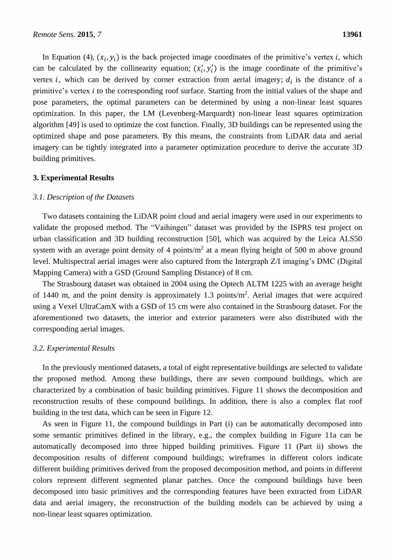
3. Experimental Results
3.1. Description of the Datasets
Two datasets containing the LiDAR point cloud and aerial imagery were used in our experiments to
validate the proposed method. The “Vaihingen” dataset was provided by the ISPRS test project on
urban classification and 3D building reconstruction [50], which was acquired by the Leica ALS50
system with an average point density of 4 points/m2 at a mean flying height of 500 m above ground
level. Multispectral aerial images were also captured from the Intergraph Z/I imaging’s DMC (Digital
Mapping Camera) with a GSD (Ground Sampling Distance) of 8 cm.
The Strasbourg dataset was obtained in 2004 using the Optech ALTM 1225 with an average height
of 1440 m, and the point density is approximately 1.3 points/m2. Aerial images that were acquired
using a Vexel UltraCamX with a GSD of 15 cm were also contained in the Strasbourg dataset. For the
aforementioned two datasets, the interior and exterior parameters were also distributed with the
corresponding aerial images.
3.2. Experimental Results
In the previously mentioned datasets, a total of eight representative buildings are selected to validate
the proposed method. Among these buildings, there are seven compound buildings, which are
characterized by a combination of basic building primitives. Figure 11 shows the decomposition and
reconstruction results of these compound buildings. In addition, there is also a complex flat roof
building in the test data, which can be seen in Figure 12.
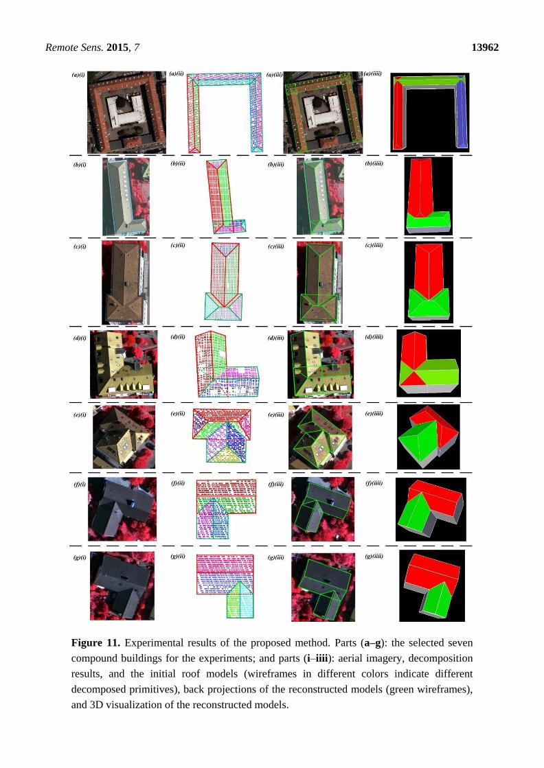
As seen in Figure 11, the compound buildings in Part (i) can be automatically decomposed into
some semantic primitives defined in the library, e.g., the complex building in Figure 11a can be
automatically decomposed into three hipped building primitives. Figure 11 (Part ii) shows the
decomposition results of different compound buildings; wireframes in different colors indicate
different building primitives derived from the proposed decomposition method, and points in different
colors represent different segmented planar patches. Once the compound buildings have been
decomposed into basic primitives and the corresponding features have been extracted from LiDAR
data and aerial imagery, the reconstruction of the building models can be achieved by using a
non-linear least squares optimization.
Remote Sens. 2015, 7 13962
Figure 11. Experimental results of the proposed method. Parts (a–g): the selected seven
compound buildings for the experiments; and parts (i–iiii): aerial imagery, decomposition
results, and the initial roof models (wireframes in different colors indicate different
decomposed primitives), back projections of the reconstructed models (green wireframes),
and 3D visualization of the reconstructed models.
Remote Sens. 2015, 7 13963
For a qualitative evaluation of the proposed method, the reconstructed 3D building models are back
projected to the corresponding aerial imagery, which are shown in Figure 11 (Part iii). As can be seen
from it, the 2D green wireframes superimposed on the aerial images are the projections of the 3D
reconstructed building models; they are located at their correct locations and coincide well with the
corresponding building edges on the aerial imagery, which means that the proposed method can
generate accurate building models. When the roof models have been reconstructed, the complete 3D
building models can be derived by extruding the roof outline to the ground when a DEM is available,
or to a ground plane with a given height. Figure 11 (Part iiii) shows the 3D visualization of the
reconstructed building models, models with different colors indicate different reconstructed primitives.
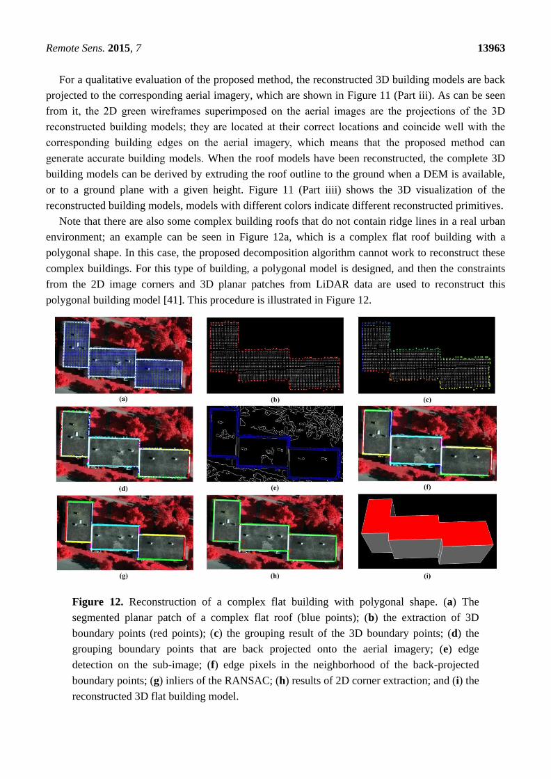
Note that there are also some complex building roofs that do not contain ridge lines in a real urban
environment; an example can be seen in Figure 12a, which is a complex flat roof building with a
polygonal shape. In this case, the proposed decomposition algorithm cannot work to reconstruct these
complex buildings. For this type of building, a polygonal model is designed, and then the constraints
from the 2D image corners and 3D planar patches from LiDAR data are used to reconstruct this
polygonal building model [41]. This procedure is illustrated in Figure 12.
Figure 12. Reconstruction of a complex flat building with polygonal shape. (a) The
segmented planar patch of a complex flat roof (blue points); (b) the extraction of 3D
boundary points (red points); (c) the grouping result of the 3D boundary points; (d) the
grouping boundary points that are back projected onto the aerial imagery; (e) edge
detection on the sub-image; (f) edge pixels in the neighborhood of the back-projected
boundary points; (g) inliers of the RANSAC; (h) results of 2D corner extraction; and (i) the
reconstructed 3D flat building model.

Remote Sens. 2015, 7 13964
After rooftop segmentation, the LiDAR points located on the same plane at different elevation
levels can be extracted, and the 2D image corners of each building can be detected with the help of
these planar patches using the following steps. First, the 3D boundary points of each planar patch are
obtained by using the modified convex hull method [51], and then these 3D boundary points are
grouped into different groups by using sleeve algorithm [14]. Red points shown in Figure 12b are the
extracted 3D boundary points and Figure 12c shows different group of boundary points. Second, the
grouped 3D boundary points were projected back to the aerial imagery and the canny detector was
applied to the aerial imagery to derive the 2D edge pixels. A buffer (15 pixels, indicating
approximately two times the point spacing) surrounding these projected boundary points was defined
to find the corresponding 2D edge pixels on the image. These are demonstrated in Figure 12d and
Figure 12e. Finally, the RANSAC algorithm was applied to each group of 2D edge pixels (Figure 12f)
to filter the irrelevant edge pixels and derive straight lines (Figure 12g), and then 2D corners can be
extracted by the intersection of the neighboring straight lines, which can be seen in Figure 12h. Once
the 2D corners have been extracted from the aerial imagery, the type of the corresponding polygonal
building model is known, and then accurate building models can be derived by using constraints from
aerial imagery and the corresponding LiDAR planar patch. Figure 12i shows the final 3D building
model reconstructed from the aforementioned procedure.
4. Discussions
4.1. Comparison Analysis of the Proposed Semantic Decomposition Method
In this section, four related building reconstruction methods based on roof topology graphs are
compared with the proposed method according to the decomposition results, and the different
decomposition results of the same compound building are used to illustrate the novelty of the proposed
method, which can be seen from Figure 13. Figure 13 (left) shows the rooftop segmentation results, the
number of the segmented planar patches and the corresponding roof topology graph, and Figure 13
(right) shows the different decomposition results (planar patches contained in each decomposition part)
and the reconstructed 3D building models.
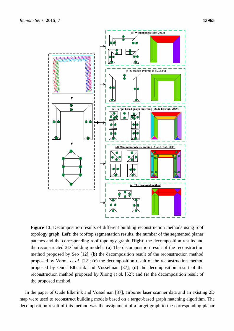
Seo [12] extracted wing models from LiDAR data by analyzing the surface patch adjacency graphs,
and then aggregated these wing models for the reconstruction of complex buildings. As can be seen
from Figure 13a, the wing models used in this method were only the combination of planar patches,
but not semantic building primitives that were familiar to people. Thus, they cannot be represented as
parametric forms to adopt a model-driven method for the reconstruction. To extract parametric models
from the LiDAR points, Verma et al. [22] defined simple roof shapes as GI, GL, and GU models, which
can be recognized by the corresponding sub-graphs. These simple roof shapes were searched from the
roof topology graphs and then reconstructed by fitting them to the point clouds. For the compound
building model in Figure 13, the decomposition result is a GU shape model in Verma et al. [22], which
is still a combination of basic building primitives (Figure 13b). This decomposition will reduce the
flexibility of the building reconstruction because it needs to define a more complicated building
primitive and then extract it using an exhaustive search.
Remote Sens. 2015, 7 13965
7
1 2
3 4
8
5 6
(a) Wing models (Seo, 2003)
6
8
5
3
4
1 2
7
1
3
4
2
6 51 2
3
4
6 5
7 8
(b) U models (Verma et al., 2006)
(c) Target based graph matching (Oude Elbrink, 2009)
(d) Minimum cycles searching (Xiong et al., 2015)
(e) The proposed method
3
4
1 2
7
3
4
6 5
8
1
3
42
3
4
1 2
1 2
7
46
3
5
56
56
8
1
3
4
24
3
56
1 2
7
56
8
1 2
7
3
4
56
8
3
1 5
3
1
3
4
2
3
5
6
4
1 2
7
6 5
8
Figure 13. Decomposition results of different building reconstruction methods using roof
topology graph. Left: the rooftop segmentation results, the number of the segmented planar
patches and the corresponding roof topology graph. Right: the decomposition results and
the reconstructed 3D building models. (a) The decomposition result of the reconstruction
method proposed by Seo [12]; (b) the decomposition result of the reconstruction method
proposed by Verma et al. [22]; (c) the decomposition result of the reconstruction method
proposed by Oude Elberink and Vosselman [37]; (d) the decomposition result of the
reconstruction method proposed by Xiong et al. [52]; and (e) the decomposition result of
the proposed method.
In the paper of Oude Elberink and Vosselman [37], airborne laser scanner data and an existing 2D
map were used to reconstruct building models based on a target-based graph matching algorithm. The
decomposition result of this method was the assignment of a target graph to the corresponding planar
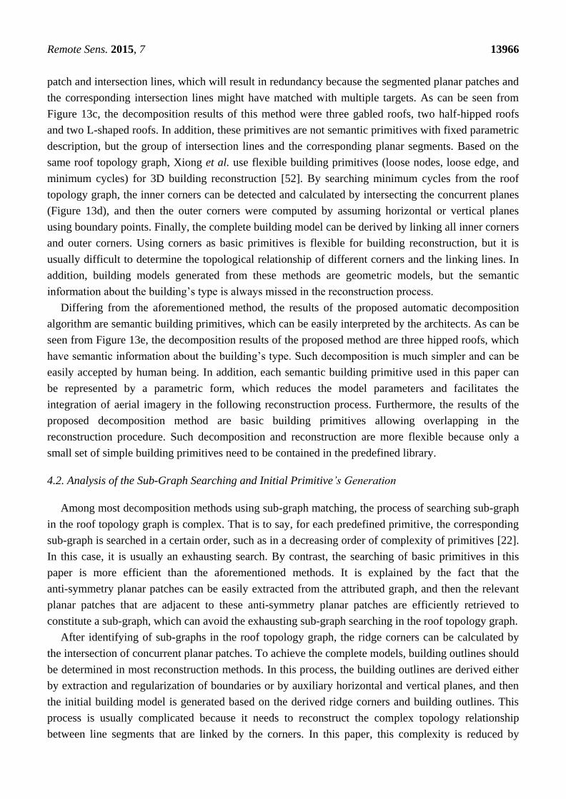
Remote Sens. 2015, 7 13966
patch and intersection lines, which will result in redundancy because the segmented planar patches and
the corresponding intersection lines might have matched with multiple targets. As can be seen from
Figure 13c, the decomposition results of this method were three gabled roofs, two half-hipped roofs
and two L-shaped roofs. In addition, these primitives are not semantic primitives with fixed parametric
description, but the group of intersection lines and the corresponding planar segments. Based on the
same roof topology graph, Xiong et al. use flexible building primitives (loose nodes, loose edge, and
minimum cycles) for 3D building reconstruction [52]. By searching minimum cycles from the roof
topology graph, the inner corners can be detected and calculated by intersecting the concurrent planes
(Figure 13d), and then the outer corners were computed by assuming horizontal or vertical planes
using boundary points. Finally, the complete building model can be derived by linking all inner corners
and outer corners. Using corners as basic primitives is flexible for building reconstruction, but it is
usually difficult to determine the topological relationship of different corners and the linking lines. In
addition, building models generated from these methods are geometric models, but the semantic
information about the building’s type is always missed in the reconstruction process.
Differing from the aforementioned method, the results of the proposed automatic decomposition
algorithm are semantic building primitives, which can be easily interpreted by the architects. As can be
seen from Figure 13e, the decomposition results of the proposed method are three hipped roofs, which
have semantic information about the building’s type. Such decomposition is much simpler and can be
easily accepted by human being. In addition, each semantic building primitive used in this paper can
be represented by a parametric form, which reduces the model parameters and facilitates the
integration of aerial imagery in the following reconstruction process. Furthermore, the results of the
proposed decomposition method are basic building primitives allowing overlapping in the
reconstruction procedure. Such decomposition and reconstruction are more flexible because only a
small set of simple building primitives need to be contained in the predefined library.
4.2. Analysis of the Sub-Graph Searching and Initial Primitive’s Generation
Among most decomposition methods using sub-graph matching, the process of searching sub-graph
in the roof topology graph is complex. That is to say, for each predefined primitive, the corresponding
sub-graph is searched in a certain order, such as in a decreasing order of complexity of primitives [22].
In this case, it is usually an exhausting search. By contrast, the searching of basic primitives in this
paper is more efficient than the aforementioned methods. It is explained by the fact that the
anti-symmetry planar patches can be easily extracted from the attributed graph, and then the relevant
planar patches that are adjacent to these anti-symmetry planar patches are efficiently retrieved to
constitute a sub-graph, which can avoid the exhausting sub-graph searching in the roof topology graph.
After identifying of sub-graphs in the roof topology graph, the ridge corners can be calculated by
the intersection of concurrent planar patches. To achieve the complete models, building outlines should
be determined in most reconstruction methods. In this process, the building outlines are derived either
by extraction and regularization of boundaries or by auxiliary horizontal and vertical planes, and then
the initial building model is generated based on the derived ridge corners and building outlines. This
process is usually complicated because it needs to reconstruct the complex topology relationship
between line segments that are linked by the corners. In this paper, this complexity is reduced by
Remote Sens. 2015, 7 13967
decomposing the compound building into simple building primitives with inherent topology
relationships among corners, line segments, and planes. As a result, the outline of each decomposed
primitive can be easily derived by using MBR algorithm, and then these initial 3D primitives can be
easily generated based on the primitive’s type, the corresponding planar patches and the 2D MBR.
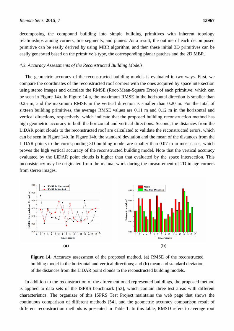
4.3. Accuracy Assessments of the Reconstructed Building Models
The geometric accuracy of the reconstructed building models is evaluated in two ways. First, we
compare the coordinates of the reconstructed roof corners with the ones acquired by space intersection
using stereo images and calculate the RMSE (Root-Mean-Square Error) of each primitive, which can
be seen in Figure 14a. In Figure 14 a, the maximum RMSE in the horizontal direction is smaller than
0.25 m, and the maximum RMSE in the vertical direction is smaller than 0.20 m. For the total of
sixteen building primitives, the average RMSE values are 0.11 m and 0.12 m in the horizontal and
vertical directions, respectively, which indicate that the proposed building reconstruction method has
high geometric accuracy in both the horizontal and vertical directions. Second, the distances from the
LiDAR point clouds to the reconstructed roof are calculated to validate the reconstructed errors, which
can be seen in Figure 14b. In Figure 14b, the standard deviation and the mean of the distances from the
LiDAR points to the corresponding 3D building model are smaller than 0.07 m in most cases, which
proves the high vertical accuracy of the reconstructed building model. Note that the vertical accuracy
evaluated by the LiDAR point clouds is higher than that evaluated by the space intersection. This
inconsistency may be originated from the manual work during the measurement of 2D image corners
from stereo images.
(a) (b)
Figure 14. Accuracy assessment of the proposed method. (a) RMSE of the reconstructed
building model in the horizontal and vertical directions; and (b) mean and standard deviation
of the distances from the LiDAR point clouds to the reconstructed building models.
In addition to the reconstruction of the aforementioned represented buildings, the proposed method
is applied to data sets of the ISPRS benchmark [53], which contain three test areas with different
characteristics. The organizer of this ISPRS Test Project maintains the web page that shows the
continuous comparison of different methods [54], and the geometric accuracy comparison result of
different reconstruction methods is presented in Table 1. In this table, RMSD refers to average root

Remote Sens. 2015, 7 13968
mean square error in the XY plane and RMSZ refers to average root mean square error in the Z
direction. The result of the proposed method is highlighted in green.
Table 1. Geometrical accuracy of different reconstruction methods in three test areas.
Researchers and References Area 1 Area 2 Area 3
RMSD (m) RMSZ (m) RMSD (m) RMSZ (m) RMSD (m) RMSZ (m)
J.Y. Rau [55] 0.9 0.6 0.5 0.7 0.8 0.6
Oude Elbrink and Vosselman [37] 0.9 0.2 1.2 0.1 0.8 0.1
Xiong et al. [39] 0.8 0.2 0.5 0.2 0.7 0.1
Perera et al. [40] 0.8 0.2 0.3 0.3 0.5 0.1
Dorninger and Pfeifer [9] 0.9 0.3 0.7 0.3 0.8 0.1
Sohn et al. [56] 0.8 0.3 0.5 0.3 0.6 0.2
Awrangjeb et al. [19] 0.9 0.2 0.7 0.3 0.8 0.1
He et al. [57] 0.7 0.2 0.6 0.3 0.7 0.2
The proposed method 0.8 0.3 0.5 0.3 0.6 0.1
As shown in Table 1, the average horizontal error and vertical error of the proposed method in three
test areas are 0.8 m and 0.3 m (Area 1), 0.5 m and 0.3 m (Area 2), 0.6 m and 0.1 m (Area 3),
respectively. Though the elevation accuracy (RMSZ) is comparable with other reconstruction methods,
the plane accuracy (RMSD) of the proposed method outperforms most of other reconstruction
methods. It is because the accurate features derived from aerial imagery can be tightly integrated into a
parameter’s optimization by decomposing the compound buildings into basic building primitives.
4.4. Uncertainties and Limitations of the Proposed Method
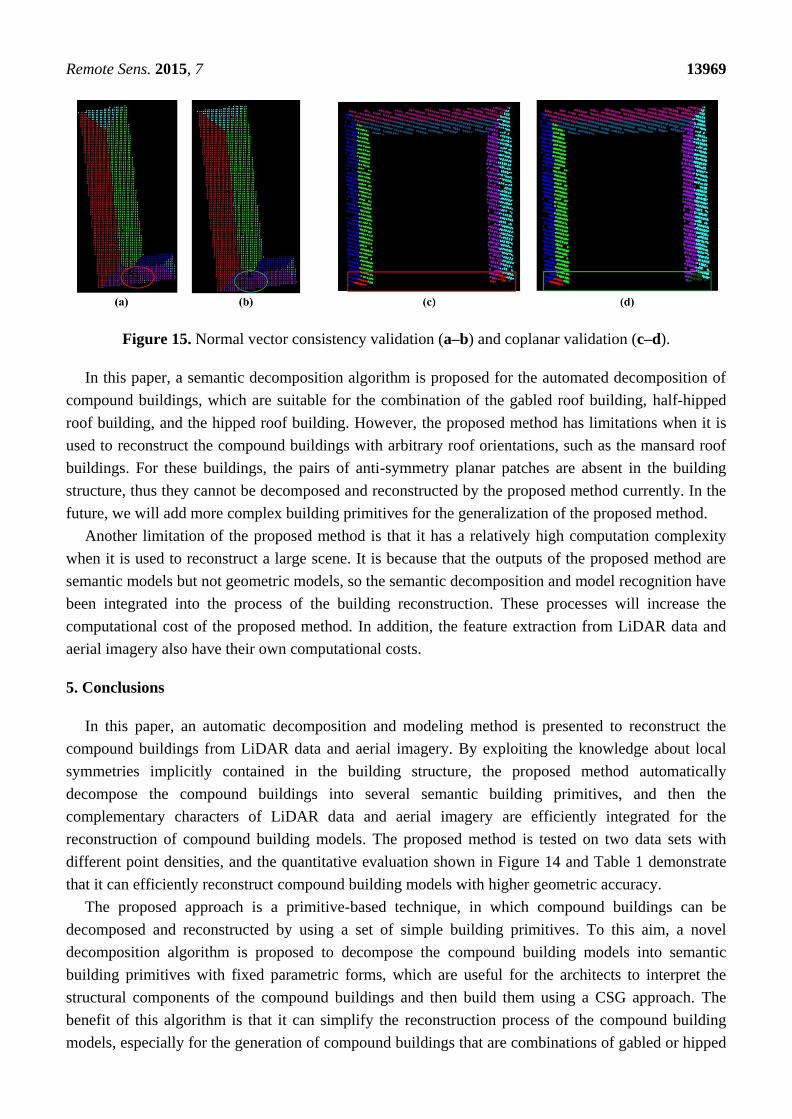
The rooftop segmentation results are important inputs for the subsequent building decomposition
and modeling. When the RANSAC algorithm is implemented in an iterative way to extract planar
patches, some LiDAR points that are not really located on the same plane can be detected. As seen in
Figure 15a, the green colored LiDAR points in the red circle are really located on the purple planar
patch, but are grouped into the green planar patch because the classic RANSAC algorithm only
considers the pure mathematical principle of the plane. In this case, the normal vector consistency
validation of the points on the extracted plane is applied. That is, the points on the extracted plane are
fit by the least-squares method, and then the discrepancy between the normal vector of each point and
the fitting plane is calculated. If the discrepancy is smaller than a predefined threshold, the point is
reserved in this planar patch. Otherwise, the point may be located on other rooftop patches and will be
put into the original building cluster for the following planar patch extraction. After the normal vector
consistency validation, the green LiDAR points in the red circle can be correctly grouped into the
corresponding planar patch, which can be seen in Figure 15b. Another problem of the rooftop
segmentation is that the extracted points are on the same mathematical planes, but are spatially separated,
as seen in the red rectangle in Figure 15c. Such coplanar patches can be separated by a connected
component analysis, as seen in Figure 15d.
Remote Sens. 2015, 7 13969
Figure 15. Normal vector consistency validation (a–b) and coplanar validation (c–d).
In this paper, a semantic decomposition algorithm is proposed for the automated decomposition of
compound buildings, which are suitable for the combination of the gabled roof building, half-hipped
roof building, and the hipped roof building. However, the proposed method has limitations when it is
used to reconstruct the compound buildings with arbitrary roof orientations, such as the mansard roof
buildings. For these buildings, the pairs of anti-symmetry planar patches are absent in the building
structure, thus they cannot be decomposed and reconstructed by the proposed method currently. In the
future, we will add more complex building primitives for the generalization of the proposed method.
Another limitation of the proposed method is that it has a relatively high computation complexity
when it is used to reconstruct a large scene. It is because that the outputs of the proposed method are
semantic models but not geometric models, so the semantic decomposition and model recognition have
been integrated into the process of the building reconstruction. These processes will increase the
computational cost of the proposed method. In addition, the feature extraction from LiDAR data and
aerial imagery also have their own computational costs.
5. Conclusions
In this paper, an automatic decomposition and modeling method is presented to reconstruct the
compound buildings from LiDAR data and aerial imagery. By exploiting the knowledge about local
symmetries implicitly contained in the building structure, the proposed method automatically
decompose the compound buildings into several semantic building primitives, and then the
complementary characters of LiDAR data and aerial imagery are efficiently integrated for the
reconstruction of compound building models. The proposed method is tested on two data sets with
different point densities, and the quantitative evaluation shown in Figure 14 and Table 1 demonstrate
that it can efficiently reconstruct compound building models with higher geometric accuracy.
The proposed approach is a primitive-based technique, in which compound buildings can be
decomposed and reconstructed by using a set of simple building primitives. To this aim, a novel
decomposition algorithm is proposed to decompose the compound building models into semantic
building primitives with fixed parametric forms, which are useful for the architects to interpret the
structural components of the compound buildings and then build them using a CSG approach. The
benefit of this algorithm is that it can simplify the reconstruction process of the compound building
models, especially for the generation of compound buildings that are combinations of gabled or hipped
Remote Sens. 2015, 7 13970
roofs. In addition, the proposed method allows the basic primitives to overlap in the decomposition
process, which can reduce the number of basic primitives in the predefined library and keep the
primitive’s integrity and regularity during the building reconstruction. As a result, the traditional model
driven methods can be further extended to the automated reconstruction of compound buildings by
using the proposed semantic decomposition method.
However, it is still a difficult task to automatically reconstruct building models with more complex
structures. In this paper, the compound buildings are assumed as a combination of simple primitives
with symmetric planar patches, which are not enough for the reconstruction of a variety of complex
buildings in reality. In the future, the non-planar roof primitives (e.g., curved structure buildings,
cones, and cylinders) will be adopted to extend the proposed method to reconstruct more complex
buildings, and the ground-based and mobile-based data will be integrated with the airborne data to
create more completed building models.
Acknowledgments
This work is supported by National Natural Science Foundation of China Grant No. 41171265,
41331171 and 40801131. This work is also supported by the National Basic Research Program of
China (973 Program) Grant No. 2013CB733402 and the Open Research Fund of Key Laboratory of
Digital Earth Science, Institute of Remote Sensing and Digital Earth, Chinese Academy of Sciences
No. 2014LDE015.
The Vaihingen data set was provided by the German Society for Photogrammetry, Remote Sensing
and Geo- information (DGPF) (Cramer, 2010): http://www.ifp.uni-stuttgart.de/dgpf/DKEP-Allg.html
(in German). The authors would also like to acknowledge the provision of the Strasbourg dataset by
Professor Pierre Grussenmeyer, INSA Strasbourg, Graduate School of Science and Technology.
Author Contributions
Hongtao Wang has proposed the semantic decomposition method, implemented and conducted the
tests on the data sets. Wuming Zhang proposed the primitive-based modeling method and guided the
research work related to this method. Yiming Chen did research on the segmentation of the buildings
and roofs. Kai Yan did research on features extraction from the aerial imagery. Mei Chen evaluated the
proposed modeling method using real data set.
Conflicts of Interest
The authors declare no conflict of interest.
References
1. Habib, A.F.; Zhai, R.; Kim, C. Generation of complex polyhedral building models by integrating
stereo-aerial imagery and LiDAR data. Photogramm. Eng. Remote Sens. 2010, 76, 609–623.
2. Haala, N.; Kada, M. An update on automatic 3D building reconstruction. ISPRS J. Photogramm.
Remote Sens. 2010, 65, 570–580.
Remote Sens. 2015, 7 13971
3. Rottensteiner, F.; Briese, C. Automatic generation of building models from LiDAR data and the
integration of aerial images. Int. Arch. Photogramm. Remote Sens. Spat. Inf. Sci. 2003, 34, 174–180.
4. Tarsha-Kurdi, F.; Landes, T.; Grussenmeyer, P. Extended RANSAC algorithm for automatic
detection of building roof planes from LiDAR data. Photogramm. J. Finl. 2008, 21, 97–109.
5. Vosselman, G.; Dijkman, S. 3D building model reconstruction from point clouds and ground
plans. Int. Arch. Photogramm. Remote Sens. Spat. Inf. Sci. 2001, 34, 37–44.
6. Xiao, Y.; Wang, C.; Li, J.; Zhang, W.; Xi, X.; Wang, C.; Dong, P. Building segmentation and
modeling from airborne LiDAR data. Int. J. Digit. Earth 2014, 5, 1–16.
7. Sampath, A.; Shan, J. Segmentation and reconstruction of polyhedral building roofs from aerial
LiDAR point clouds. IEEE Trans. Geosci. Remote Sens. 2010, 48, 1554–1567.
8. Zhou, Q.Y.; Neumann, U. 2.5D building modeling by discovering global regularities. In
Proceedings of the 2012 IEEE Conference on Computer Vision and Pattern Recognition(CVPR),
Providence, RI, USA, 16–21 June 2012; pp. 326–333.
9. Dorninger, P.; Pfeifer, N. A comprehensive automated 3D approach for building extraction,
reconstruction, and regularization from airborne laser scanning point clouds. Sensors 2008, 8,
7323–7343.
10. You, H.J.; Zhang, S.Q. 3D building reconstruction from aerial CCD image and sparse laser
sample data. Opt. Lasers Eng. 2006, 44, 555–566.
11. Sohn, G.; Dowman, I. Data fusion of high-resolution satellite imagery and LiDAR data for
automatic building extraction. ISPRS J. Photogramm. Remote Sens. 2007, 62, 43–63.
12. Seo, S. Model-Based Automatic Building Extraction from LiDAR and Aerial Imagery. Ph.D.
Thesis, The Ohio State University, Columbus, OH, USA, 2003.
13. Rottensteiner, F.; Trinder, J.; Clode, S.; Kubik, K. Fusing airborne laser scanner data and aerial
imagery for the automatic extraction of buildings in densely built-up areas. Int. Arch.
Photogramm. Remote Sens. 2004, 35, 512–517.
14. Ma, R. Building Model Reconstruction from LiDAR Data and Aerial Photographs. Ph.D. Thesis,
The Ohio State University, Columbus, OH, USA, 2004.
15. Kim, C.J.; Habib, A. Object-based integration of photogrammetric and LiDAR data for automated
generation of complex polyhedral building models. Sensors 2009, 9, 5679–5701.
16. Cheng, L.A.; Gong, J.Y.; Li, M.C.; Liu, Y.X. 3D building model reconstruction from multi-view
aerial imagery and LiDAR data. Photogramm. Eng. Remote Sens. 2011, 77, 125–139.
17. Chen, L.C.; Teo, T.A.; Shao, Y.C.; Lai, Y.C.; Rau, J.Y. Fusion of LiDAR data and optical
imagery for building modeling. Int. Arch. Photogramm. Remote Sens. 2004, 35, 732–737.
18. Kwak, E. Automatic 3D Building Model Generation by Integrating LiDAR and Aerial Images
Using a Hybrid Approach. Ph.D. Thesis, University of Calgary, Calgary, AB, Canada, 2013.
19. Awrangjeb, M.; Zhang, C.S.; Fraser, C.S. Automatic extraction of building roofs using LiDAR
data and multispectral imagery. ISPRS J. Photogramm. Remote Sens. 2013, 83, 1–18.
20. Brenner, C. Constraints for modelling complex objects. Int. Arch. Photogramm. Remote Sens.
Spat. Inf. Sci. 2005, 36, 49–54.

Remote Sens. 2015, 7 13972
21. Brenner, C. Modelling 3D objects using weak CSG primitives. Int. Arch. Photogramm. Remote
Sens. Spat. Inf. Sci. 2004, 35, 1085–1090.
22. Verma, V.; Kumar, R.; Hsu, S. 3D building detection and modeling from aerial LiDAR data. In
Proceedings of the 2006 IEEE Conference on Computer Vision and Pattern Recognition(CVPR),
New York, NY, USA, 17–22 June 2006; pp. 2213–2220.
23. Maas, H.G.; Vosselman, G. Two algorithms for extracting building models from raw laser
altimetry data. ISPRS J. Photogramm. Remote Sens. 1999, 54, 153–163.
24. Kada, M.; McKinley, L. 3D building reconstruction from lidar based on a cell decomposition
approach. Int. Arch. Photogramm. Remote Sens. Spat. Inf. Sci. 2009, 38, 47–52.
25. Henn, A.; Groger, G.; Stroh, V.; Plumer, L. Model driven reconstruction of roofs from sparse
LiDAR point clouds. ISPRS J. Photogramm. Remote Sens. 2013, 76, 17–29.
26. Haala, N.; Brenner, C. Extraction of buildings and trees in urban environments. ISPRS J.
Photogramm. Remote Sens. 1999, 54, 130–137.
27. Tseng, Y.H.; Wang, S.D. Semi-automated building extraction based on CSG model-image fitting.
Photogramm. Eng. Remote Sens. 2003, 69, 171–180.
28. Suveg, D.; Vosselman, G. Reconstruction of 3D building models from aerial images and maps.
ISPRS J. Photogramm. Remote Sens. 2004, 58, 202–224.
29. Lafarge, F.; Descombes, X.; Zerubia, J.; Pierrot-Deseilligny, M. Structural approach for building
reconstruction from a single DSM. IEEE Trans. Pattern Anal. Mach. Intell. 2008, 32, 135–147.
30. Huang, H.; Brenner, C.; Sester, M. A generative statistical approach to automatic 3D building roof
reconstruction from laser scanning data. ISPRS J. Photogramm. Remote Sens. 2013, 79, 29–43.
31. Vosselman, G.; Veldhuis, H. Mapping by dragging and fitting of wire-frame models.
Photogramm. Eng. Remote Sens. 1999, 65, 769–776.
32. Durupt, M.; Taillandier, F. Automatic building reconstruction from a digital elevation model and
cadastral data: An operational approach. Int. Arch. Photogramm. Remote Sens. Spat. Inf. Sci.
2006, 36, 142–147.
33. Wang, S.; Tseng, Y.H. Least squares model image fitting of floating models for building
extraction from images. J. Chin. Inst. Eng. 2009, 32, 667–677.
34. Gruen, A.; Wang, X. Cc-modeler: A topology generator for 3D city models. ISPRS J.
Photogramm. Remote Sens. 1998, 53, 286–295.
35. Wang, S.; Tseng, Y.H.; Chen, L.C. Semi-automated model-based building reconstruction by
fitting models to versatile data. In Proceedings of the 29th Asian Conference on Remote Sensing,
Colombo, Sri Lanka, 10–14 November 2008.
36. Haala, N.; Becker, S.; Kada, M. Cell decomposition for the generation of building models at
multiple scales. Int. Arch. Photogramm. Remote Sens. Spat. Inf. Sci. 2006, 36, 19–24.
37. Oude Elberink, S.; Vosselman, G. Building reconstruction by target based graph matching on
incomplete laser data: Analysis and limitations. Sensors 2009, 9, 6101–6118.
38. Lin, H.; Gao, J.Z.; Zhou, Y.; Lu, G.L.; Ye, M.; Zhang, C.X.; Liu, L.G.; Yang, R.G. Semantic
decomposition and reconstruction of residential scenes from LiDAR data. ACM Trans. Graph.
2013, 32, 6601–6610.
Remote Sens. 2015, 7 13973
39. Xiong, B.; Oude Elberink, S.; Vosselman, G. A graph edit dictionary for correcting errors in roof
topology graphs reconstructed from point clouds. ISPRS J. Photogramm. Remote Sens. 2014, 93,
227–242.
40. Perera, G.S.N.; Maas, H.G. Cycle graph analysis for 3D roof structure modelling: Concepts and
performance. ISPRS J. Photogramm. Remote Sens. 2014, 93, 213–226.
41. Zhang, W.; Wang, H.; Chen, Y.; Yan, K.; Chen, M. 3D building roof modeling by optimizing
primitive’s parameters using constraints from lidar data and aerial imagery. Remote Sens. 2014, 6,
8107–8133.
42. Axelsson, P. DEM generation from laser scanner data using adaptive TIN models. Int. Arch.
Photogramm. Remote Sens. 2000, 33, 111–118.
43. Rusu, R.B. Semantic 3D object maps for everyday manipulation in human living environments.
Künstl. Intell. 2010, 24, 345–348.
44. Chen, D.; Zhang, L.; Li, J.; Liu, R. Urban building roof segmentation from airborne LiDAR point
clouds. Int. J. Remote Sens. 2012, 33, 6497–6515.
45. Edelsbrunner, H.; Kirkpatrick, D.; Seidel, R. On the shape of a set of points in the plane. IEEE
Trans. Inf. Theory 1983, 29, 551–559.
46. Chaudhuri, D.; Samal, A. A simple method for fitting of bounding rectangle to closed regions.
Pattern Recognit. 2007, 40, 1981–1989.
47. Canny, J. A computational approach to edge detection. IEEE Trans. Pattern Anal. Mach. Intell.
1986, 8, 679–698.
48. Fischler, M.A.; Bolles, R.C. Random sample consensus: A paradigm for model fitting with
applications to image analysis and automated cartography. Commun. ACM 1981, 24, 381–395.
49. Marquardt, D.W. An algorithm for least-squares estimation of nonlinear parameters. J. Soc. Ind.
Appl. Math. 1963, 11, 431–441.
50. ISPRS Test Project on Urban Classification and 3D Building Reconstruction. Available online:
http://www.itc.nl/isprs_wgiii4/docs/complexscenes.pdf (accessed on 7 August 2015).
51. Sampath, A.; Shan, J. Building boundary tracing and regularization from airborne LiDAR point
clouds. Photogramm. Eng. Remote Sens. 2007, 73, 805–812.
52. Xiong, B.; Jancosek, M.; Oude Elberink, S.; Vosselman, G. Flexible building primitives for 3D
building modeling. ISPRS J. Photogramm. Remote Sens. 2015, 101, 275–290.
53. Rottensteiner, F.; Sohn, G.; Gerke, M.; Wegner, J.D.; Breitkopf, U.; Jung, J. Results of the ISPRS
benchmark on urban object detection and 3D building reconstruction. ISPRS J. Photogramm.
Remote Sens. 2013, 93, 256–271.
54. ISPRS Test Project on Urban Classification and 3D Building Reconstruction: Results. Available
online: http://brian94.de/ISPRSIII_4_Test_results/tests_datasets_results_main.html (accseesed on
30 July 2015).
55. Rau, J.Y. A line-based 3D roof modell reconstruction algorithm: TIN-merging and reshaping
(TMR). In Proceedings of the ISPRS Annals of the Photogrammetry, Remote Sensing and Spatial
Information Sciences, Melbourne, Australia, 25 August–1 September 2012; pp. 287–292.
Remote Sens. 2015, 7 13974
56. Sohn, G.; Huang, X.F.; Tao, V. Using a binary space partitioning tree for reconstructing
polyhedral building models from airborne LiDAR data. Photogramm. Eng. Remote Sens. 2008,
74, 1425–1438.
57. He, Y.; Zhang, C.; Fraser, C. A line-based spectral clustering method for efficient planar structure
extraction from lidar data. In Proceedings of ISPRS Annals of the Photogrammetry, Remote
Sensing and Spatial Information Sciences, Antalya, Turkey, 11–13 November 2013; pp. 103–108.
© 2015 by the authors; licensee MDPI, Basel, Switzerland. This article is an open access article
distributed under the terms and conditions of the Creative Commons Attribution license
(http://creativecommons.org/licenses/by/4.0/).