Embed Size (px)
Citation preview
Selmer Groups and Galois Representations
Edray Herber Goins
July 31, 2016

2

Contents
1 Galois Cohomology 7
1.1 Notation . . . . . . . . . . . . . . . . . . . . . . . . . . . . . . . . . . . . . . . . . . . 8
2 Galois Groups as Topological Spaces 9
2.1 Abstract Algebra Review . . . . . . . . . . . . . . . . . . . . . . . . . . . . . . . . . 9
2.1.1 Commutative Groups . . . . . . . . . . . . . . . . . . . . . . . . . . . . . . . 9
2.1.2 Fields . . . . . . . . . . . . . . . . . . . . . . . . . . . . . . . . . . . . . . . . 10
2.1.3 Galois Theory . . . . . . . . . . . . . . . . . . . . . . . . . . . . . . . . . . . . 10
2.2 Profinite Groups as Topological Spaces . . . . . . . . . . . . . . . . . . . . . . . . . . 11
2.2.1 Absolute Galois Groups . . . . . . . . . . . . . . . . . . . . . . . . . . . . . . 11
2.2.2 Krull Topology . . . . . . . . . . . . . . . . . . . . . . . . . . . . . . . . . . . 11
2.2.3 Profinite Groups . . . . . . . . . . . . . . . . . . . . . . . . . . . . . . . . . . 12
2.2.4 Example: `-adic Numbers . . . . . . . . . . . . . . . . . . . . . . . . . . . . . 13
3 G-Modules and X-Torsors 15
3.1 Galois Modules . . . . . . . . . . . . . . . . . . . . . . . . . . . . . . . . . . . . . . . 15
3.1.1 Abelian Groups with Continuous Galois Action . . . . . . . . . . . . . . . . . 15
3.1.2 Example: Additive Group Ga and Multiplicative Group Gm . . . . . . . . . . 15
3.1.3 Example: Elliptic Curves . . . . . . . . . . . . . . . . . . . . . . . . . . . . . 16
3.1.4 Tate Modules . . . . . . . . . . . . . . . . . . . . . . . . . . . . . . . . . . . . 17
3.1.5 Isogenies of Galois Modules . . . . . . . . . . . . . . . . . . . . . . . . . . . . 19
3.1.6 Sheaves of Galois Modules . . . . . . . . . . . . . . . . . . . . . . . . . . . . . 20
3.1.7 Principal Homogeneous Spaces . . . . . . . . . . . . . . . . . . . . . . . . . . 22
3.1.8 Torsors via Translation Maps . . . . . . . . . . . . . . . . . . . . . . . . . . . 24
3.1.9 Example: Quadratic Curves . . . . . . . . . . . . . . . . . . . . . . . . . . . . 25
3.1.10 Example: Cubic Curves . . . . . . . . . . . . . . . . . . . . . . . . . . . . . . 27
3.2 Selmer’s Cubic . . . . . . . . . . . . . . . . . . . . . . . . . . . . . . . . . . . . . . . 27
3.2.1 Example: Quartic Curves . . . . . . . . . . . . . . . . . . . . . . . . . . . . . 29
3.2.2 Elliptic Curves: 2-Isogeny . . . . . . . . . . . . . . . . . . . . . . . . . . . . . 32
3.2.3 Elliptic Curves: 2-Torsion . . . . . . . . . . . . . . . . . . . . . . . . . . . . . 32
4 Galois Cohomology 35
4.1 Continuous Maps . . . . . . . . . . . . . . . . . . . . . . . . . . . . . . . . . . . . . . 35
4.1.1 Sections . . . . . . . . . . . . . . . . . . . . . . . . . . . . . . . . . . . . . . . 35
4.1.2 Cochain Complexes . . . . . . . . . . . . . . . . . . . . . . . . . . . . . . . . 36
3

4.1.3 Where are these maps coming from? . . . . . . . . . . . . . . . . . . . . . . . 384.1.4 Example: Free G-Modules . . . . . . . . . . . . . . . . . . . . . . . . . . . . . 384.1.5 Cohomology Groups . . . . . . . . . . . . . . . . . . . . . . . . . . . . . . . . 38
4.2 Weil-Chatalet Groups . . . . . . . . . . . . . . . . . . . . . . . . . . . . . . . . . . . 394.2.1 Example: Hilbert’s Theorem 90 . . . . . . . . . . . . . . . . . . . . . . . . . . 41
4.3 Cup Product . . . . . . . . . . . . . . . . . . . . . . . . . . . . . . . . . . . . . . . . 414.4 Long Exact Sequence for Cohomology . . . . . . . . . . . . . . . . . . . . . . . . . . 43
4.4.1 Example: Kummer Theory . . . . . . . . . . . . . . . . . . . . . . . . . . . . 454.4.2 Example: Elliptic Curve . . . . . . . . . . . . . . . . . . . . . . . . . . . . . . 454.4.3 Example: Weil Pairing . . . . . . . . . . . . . . . . . . . . . . . . . . . . . . . 45
4.5 Pushforward on Cohomology . . . . . . . . . . . . . . . . . . . . . . . . . . . . . . . 464.5.1 Example: Decomposition and Inertia Groups . . . . . . . . . . . . . . . . . . 48
I Selmer Groups 514.6 History . . . . . . . . . . . . . . . . . . . . . . . . . . . . . . . . . . . . . . . . . . . 53
4.6.1 Lind and Reichardt’s Quartic . . . . . . . . . . . . . . . . . . . . . . . . . . . 534.7 Selmer and Shafarevich-Tate Groups . . . . . . . . . . . . . . . . . . . . . . . . . . . 56
4.7.1 Classical Definitions . . . . . . . . . . . . . . . . . . . . . . . . . . . . . . . . 564.7.2 Elliptic Curves . . . . . . . . . . . . . . . . . . . . . . . . . . . . . . . . . . . 57
4

List of Figures
3.1 A Geometric Proof of the Associativity of the Group Law . . . . . . . . . . . . . . . 18
5

6

7
Chapter 1
Galois Cohomology
1.1 Notation
k, F , K, L Fields
k A separable, algebraic closure of k
I A partially ordered set(G, ◦
)Absolute Galois group, namely Gal(k/k), with composition ◦ : G×G→ G(
Γ, ◦)
A profinite group
U Open subgroup of G
U , V , W Open sets in G
σ, τ , ν, ω Elements of G(X, ⊕, }
)G-module with maps ⊕ : X ×X → X and } : G×X → X
P , Q, R Elements of X
O Identity element of X(Y, �, �
)Principal homogeneous space with maps � : X × Y → Y and � : G× Y → Y
Q, R Elements of Y
f Bijection X → Y from G-module to a principal homogeneous space
g Bijection Y → Z between principal homogeneous spaces
{Y/X} Equivalence class of principal homogeneous spaces Z ∼ YE, E′ Elliptic curves
φ, φ′ Dual m-isogenies φ : E′ → E and φ′ : E → E′
Cn(G,X) All continuous maps G× · · · ×G→ X
ξ, α, β Elements of Cn(G,X)
∂n Boundary map Cn(G,X)→ Cn+1(G,X)
Zn(G,X) Kernel of ∂n, i.e., the n-cocycles
Bn(G,X) Image of ∂n−1, i.e., the n-coboundaries
Hn(G,X) nth cohomology group, as Zn(G,X)/Bn(G,X)
WC(E/k) Weil-Chatalet group of E, as H1(Gal(k/k
), E(k)
)f∗ Pushforward Hn(G,X)→ Hn(G, Y ) of the map f : X → Y
δn Connecting homomorphism Hn(G,X)→ Hn+1(G,X)
ϕ∗ Pullback Hn(G,X)→ Hn(Γ, X) of the map ϕ : Γ→ G
8

Chapter 2
Galois Groups as Topological Spaces
2.1 Abstract Algebra Review
2.1.1 Commutative Groups
Let X be a set. We say that X is a commutative group or an abelian group if there exists awell-defined binary operation ⊕ : X ×X → X such that
• (Associativity)(P ⊕Q
)⊕R = P ⊕
(Q⊕R
)for all P, Q, R ∈ X.
• (Commutativity) P ⊕Q = Q⊕ P for all P, Q ∈ X.
• (Identity) There exists a unique O ∈ X such that O ⊕ P = P for all P ∈ X.
• (Inverses) For each P ∈ X there exists a unique −P ∈ X such that P ⊕ (−P ) = O.
Say that(X, ⊕
),(Y, ⊕
), and
(Z, ⊕
)are commutative groups. A map f : X → Y is a homomor-
phism if f(P ⊕ Q) = f(P ) � f(Q) for all P, Q ∈ X. Define the kernel, image, and cokernel of ahomomorphism as, respectively,
ker f ={P ∈ X
∣∣ f(P ) = O}
= X[f ]
im f ={Q ∈ Y
∣∣Q = f(P ) for some P ∈ X}
= f(X)
coker f ={Q = Q� im f
∣∣Q ∈ Y } = Y/im f
(2.1.1)
If g : Y → Z is another homomorphism, we say that the composition of maps
Xf−−−−→ Y
g−−−−→ Z (2.1.2)
is an exact sequence if im f = ker g as subsets of Y . The following is a well-known result abouthomomorphisms between commutative groups which we state without proof.
Proposition 2.1.1. Say that f : X → Y is a homomorphism of commutative groups X and Y .
1. f(O) = O and f(−P ) = −f(P ) for all P ∈ X.
2.(ker f, ⊕
),(im f, ⊕
), and
(coker f, ⊕
)are commutative groups.
9
3. The following is an exact sequence:
{O} −−−−→ ker f −−−−→ Xf−−−−→ Y −−−−→ coker f −−−−→ {O} (2.1.3)
For example,(Z, +
)is a commutative group under addition with identity 0. For any integer n, the
map f : Z→ Z defined by a 7→ na is a homomorphism. The kernel and image are ker f = {0} andim f = nZ, respectively. In particular, coker f = Z/nZ is a commutative group under addition.
2.1.2 Fields
Let k be a set. We say that k is a field if there are well-defined binary operations + : k × k → kand · : k × k → k such that
• (Addition) Ga(k) = k is a commutative group under addition + with identity 0.
• (Multiplication) Gm(k) = k−{0} is a commutative group under multiplication · with identity1.
• (Distributivity) a ·(b+ c
)=(a · b
)+(a · c
)for all a, b, c ∈ k.
The sets of rational numbers Q, real numbers R, complex numbers C, and residue classes moduloa prime Fp = Z/pZ are each examples of fields. For any field k, exists an integer n such that theideal nZ is the kernel of the morphism
Z→ k defined by m 7→
1 + · · ·+ 1︸ ︷︷ ︸m times
if m > 0;
(−1) + · · ·+ (−1)︸ ︷︷ ︸|m| times
if m < 0; and
0 if m = 0.
(2.1.4)
We call |n| the characteristic of k. For example, the sets of rational numbers Q, real numbers R,complex numbers C each have characteristic 0, whereas the set of residue classes modulo a primeFp has characteristic p.
2.1.3 Galois Theory
Let k be a field. The polynomial ring R = k[x1, . . . , xn] is a unique factorization domain. We saythat a field K is a normal, separable extension of k if (1) k ⊂ K and K is the splitting field of afamily of polynomials in R not having repeated roots. Define Aut and Emb!
Let L be a normal, separable extension of k. Denote G = Gal(L/k) = Aut(L/k) = Emb(L/k)as its Galois group.
• Say that K is a subfield of L containing k; then K is a separable extension of k. Let H denoteall σ ∈ G such that σ(a) = a for all a ∈ K. Then H is a subgroup of G, and H = Gal(L/K).
• Conversely, say that H is a subgroup of G. Let K denote all a ∈ L such that σ(a) = a for allσ ∈ H. Then K is a subfield of L, and K = LH .
• In either case, K is a normal extension of k if and only if H is a normal subgroup of G.
10

2.2 Profinite Groups as Topological Spaces
2.2.1 Absolute Galois Groups
Let k be a field, and denote k as a separable, algebraic closure of k. (In practice, we will choose kas either the rational numbers Q, a completion Qv, or a finite field Fp.) We define G = Gal
(k/k
)as follows. Let Ik denote the category of finite, normal, separable extensions K of k with themorphisms being set inclusion: F ↪→ K ↪→ L. We have a directed family of groups given byrestriction of the action to subfields:
projL/F : Gal(L/k)projL/K−−−−−→ Gal(K/k)
projK/F−−−−−→ Gal(F/k) (2.2.1)
Define the projective limit as
Gal(k/k
)= lim←−
K
Gal(K/k) =
(. . . , σK , . . . ) ∈∏K∈Ik
Gal(K/k)
∣∣∣∣∣∣ projL/K(σL) = σK
(2.2.2)
It is easy to check that this is a group under composition. Since G = Gal(k/k
)is the projective
limit of finite groups Gal(K/k) we say that G is a profinite group. It may be useful to think of thisusing the following commutative diagram:
Gal(k/k
)projL
ssprojK��
projF
++Gal(L/k)
projL/K // Gal(K/k)projK/F // Gal(F/k)
(2.2.3)
2.2.2 Krull Topology
We may turn G into a topological space using the Krull topology : We say that a subgroup U ⊆ Gis open if it has finite index in G. (One may think of this as an open ball centered at the origin.)In general, we say that a subset V ⊆ G is open if for each σ ∈ V we can find a subgroup Uσ offinite index in G such that the coset σ ◦ Uσ is contained in V . (One may think of this coset as anopen ball centered at σ.) Here is a standard result:
Theorem 2.2.1. For any field k, denote its absolute Galois group as G = Gal(k/k
).
1. Both ∅ and G are open. The union⋃α Vα of arbitrarily many open sets is open. The inter-
section⋂α Vα of finitely many open sets is open.
2. Let U ⊆ G be a subgroup of finite index. Then each coset σ ◦ U is both open and closed.
3. The maps G × G → G and G → G defined as (σ, τ) 7→ σ ◦ τ and σ 7→ σ−1, respectively, arecontinuous.
4. G is a topological group which is Hausdorff, totally disconnected, and compact.
Proof. Clearly ∅ and G are open. Fix σ in an arbitrary union V =⋃α Vα. Then σ ∈ Vα for some α,
so that σ ◦Uσ ⊆ Vα for some open subgroup Uσ. As σ ◦Uσ ⊆ V , we see that that V must be open.Similarly, fix σ in a finite intersection V =
⋂α Vα. Then σ ∈ Vα for each α, so that σ ◦ Uσ,α ⊆ Vα
11
for some open subgroups Uσ,α. Denote Uα =⋂α Uσ,α. As the index |G : Uσ| ≤
∏α |G : Uσ,α| is
finite and σ ◦Uσ ⊆ V , we see that the intersection of finitely many open sets must be open as well.
Let U ⊆ G is an open subgroup, and denote V = σ ◦ U . As τ ◦ U = V for each τ ∈ V , we seethat V is open. Since U has finite index in G, we have a finite disjoint union G =
⋃ni=1
(σi ◦ U
).
As V = σj ◦ U for some j, the compliment G− V =⋃i 6=j(σi ◦ U
)is the union of open sets, we see
that V is closed.
We show that multiplication and inverses are continuous maps. Fix an open set W ⊆ G. Fix(σ, τ) in the inverse image V =
{(σ, τ
)∈ G×G
∣∣σ ◦ τ ∈W}. We can find an open subgroup Uσ◦τin W such that
(σ ◦ τ
)◦ Uσ◦τ ⊆ W . Denote the open subgroup Uσ,τ =
(τ ◦ Uσ◦τ ◦ τ−1
)× Uσ◦τ
in G × G. It is easy to see that (σ, τ) ◦ Uσ,τ ⊆ V , so that V is indeed open. Similarly, fix σ inthe inverse image V =
{σ ∈ G
∣∣σ−1 ∈W}
. We can find an open subgroup Uσ−1 in W such thatσ−1 ◦ Uσ−1 ⊆ W . Denote the open subgroup Uσ = σ−1 ◦ Uσ−1 ◦ σ in G. It is easy to see thatσ ◦ Uσ ⊆ V , so that V is indeed open.
Clearly G is a topological group. We show that G is both Hausdorff and totally disconnected.Choose distinct σ1 and σ2 in a subset S ⊆ G. As
(σ−1
1 ◦ σ2
)6= 1, there exists a finite, normal,
separable extension K of k such that(σ−1
1 ◦ σ2
)does not lie in the kernel U = ker projK of the
canonical projection projK : G→ Gal(K/k). As(σ1 ◦U
)∩(σ2 ◦U
)= ∅ we see that σ1 and σ2 can
be “housed ofh’ into disjoint open sets. Similarly, as S =⋃σα∈G/U Sα is a nontrivial disjoint union
of subsets Sα =(σα ◦ U
)∩ S, we see that S is disconnected in the subspace topology.
Finally, we show that G is compact. As each finite group Gal(K/k) is compact in the finitetopology, Tychonoff’s Compactness Theorem states that the product
∏K∈Ik Gal(K/k) is also com-
pact in the product topology. It suffices then to show that G ⊆∏K∈Ik Gal(K/k) is closed, which
we do by showing that every “convergent sequence” in G has a limit in G. To this end, let I bea totally ordered set. We say that a subset {σα |α ∈ I} ⊆ G is a Cauchy sequence if, given anopen subgroup U ⊆ G, we can find NU ∈ I such that σ−1
β ◦ σα ∈ U whenever α, β ≥ NU . In
particular, σα ∈⋂β≥NU
(σβ ◦ U
)is contained in the intersection of closed sets, so that the subse-
quence {σα |α ≥ NU} is contained in a closed subset of G. Hence must have an accumulation pointσ = limα σα in G.
Any subgroup U of finite index in G contains a normal subgroup U ′ =⋂τ∈G
(τ−1 ◦ U ◦ τ
)also
of finite index. Hence we may as well define an open subgroup as one which is a normal subgroupof finite index. In this case, the quotient group G/U ' Gal(K/k) for some finite, normal, separableextension K of k, which shows that by definition G ' lim←−U (G/U). (Often we abuse notation and
say U = Gal(k/K).)
2.2.3 Profinite Groups
In general, let I be some partially ordered set, and say that we have a collection of finite groups{Γα∣∣α ∈ I}. This is a directed family of groups whenever we have a collection of compatible group
homomorphisms
projγ,α : Γγprojγ,β−−−−→ Γβ
projβ,α−−−−→ Γα (2.2.4)
whenever α ≤ β ≤ γ. Define the projective limit as
Γ = lim←−α
Γα =
{(. . . , gα, . . . ) ∈
∏α∈I
Γα
∣∣∣∣∣ projβ,α(gβ) = gα
}(2.2.5)
12

Using the ideas from above, it is easy to check that this is a group under composition. As Γ is theprojective limit of finite groups, we say that Γ is a profinite group. In fact, Γ is a topological groupwhich is Hausdorff, totally disconnected, and compact. Serre, in his “Galois cohomology”, showsthe converse: If Γ is a topological group which is Hausdorff, totally disconnected, and compact,then G is the projective limit of of finite groups.
2.2.4 Example: `-adic Numbers
Fix a prime `. Denote I = {1, 2, . . . } = Z>0 as the collection of positive integers. For each positiveinteger α ∈ I, the subset `α Z is an additive subgroup of the integers Z which is also closed undermultiplication. The quotients Γα = Z/`α Z are then finite abelian groups. We have projectionmaps
projβ,α : Z/`β Z→ Z/`α Z which sends a mod `β 7→ a mod `α (2.2.6)
whenever α ≤ β. We define the set
Z` = lim←−α
Z/`α Z =
{(. . . , aα, . . . ) ∈
∏α∈I
Z/`α Z
∣∣∣∣∣ aβ ≡ aα mod `α
}(2.2.7)
It is easy to check thatΓα = Z/`α Z ' Z`/`α Z` for any α ∈ I. (2.2.8)
It is easy to show that Z` is a ring; we call it the collection of `-adic integers. The quotient fieldQ` is the collection of `-adic numbers.
13

14

Chapter 3
G-Modules and X-Torsors
3.1 Galois Modules
3.1.1 Abelian Groups with Continuous Galois Action
Continue to denote G = Gal(k/k
)as above. Let X be a set. (In practice, X is a subset of the
multiplicative group k×
or a subset of E(k) for some elliptic curve defined over k.) We say thatX is a G-module or a Galois module over k if there exist binary operations ⊕ : X ×X → X and} : G×X → X such that
• (Associativity)(P ⊕Q
)⊕R = P ⊕
(Q⊕R
)and
(σ ◦ τ
)} P = σ }
(τ } P
)for all σ, τ ∈ G
and P, Q, R ∈ X.
• (Commutativity) P ⊕Q = Q⊕ P for all P, Q ∈ X.
• (Distributivity) σ }(P ⊕Q
)=(σ } P
)⊕(σ }Q
)for all σ ∈ G and P, Q ∈ X.
• (Identity) There exists a unique O ∈ X such that O ⊕ P = 1} P = P for all P ∈ X.
• (Inverses) For each P ∈ X there exists a unique −P ∈ X such that P ⊕ (−P ) = O.
• (Continuity) For each P ∈ X, the stabilizer V ={σ ∈ G
∣∣σ } P = P}
of P is open.
To be more precise, we may also say X is a Z[G]-module on which G acts continuously, wherewe view X as a topological space via the discrete topology. Condition (Continuity) needs furtherexplanation: The set U ⊆ V ⊆ G is the kernel of the permutation representation G → Aut(X)defined as that map which sends σ to the homomorphism P 7→ σ } P . Hence U is a normalsubgroup of G; the condition (Continuity) assumes its index is finite. As each P ∈ X is containedin some subset
XU ={P ∈ X
∣∣σ } P = P for all σ ∈ U}
(3.1.1)
corresponding to some normal, open subgroup U ⊆ G, we have X =⋃U X
U .
3.1.2 Example: Additive Group Ga and Multiplicative Group Gm
Say that X = Ga(k) = k under ⊕ = + or X = Gm(k) = k − {0} under ⊕ = ·. The absoluteGalois group G = Gal
(k/k
)acts in the canonical way; denote this action by the binary operation
} : G×X → X. We show that X is a G-module.
15
It is easy to see that axioms (Associativity), (Commutativity), (Distributivity), (Identity), and(Inverses) are satisfied. It suffices to show that axiom (Continuity) is safisfied: Choose P ∈ X,and let V ⊆ G denote its stabilizer. As this is an element of k, it lies in some finite, normalseparable extension K of k. Denote the open subgroup U = ker projK as the kernel of the canonicalprojection projK : G → Gal(K/k). It is easy to see that the coset σ ◦ U acts trivially on P forany σ ∈ V . Hence σ ◦ U ⊆ V , so we see that V is indeed open. (Note that XU = Ga(K) = K orXU = Gm(K) = K − {0}, respectively, so that X =
⋃U X
U .)
3.1.3 Example: Elliptic Curves
Fix coefficients a1, a2, a3, a4, a6 ∈ k, and consider the homogeneous cubic polynomial
f(x1, x2, x0) =(x2
2 x0 + a1 x1 x2 x0 + a3 x2 x20
)−(x3
1 + a2 x21 x0 + a4 x1 x
20 + a6 x
30
). (3.1.2)
For each normal, separable extension K of k we denote the set
E(K) =
{(x1 : x2 : x0) ∈ P2(K)
∣∣∣∣ f(x1, x2, x0) = 0
}'{
(x, y) ∈ A2(K)
∣∣∣∣ y2 + a1 x y + a3 = x3 + a2 x2 + a4 x+ a6
}∪ {O}
(3.1.3)
in terms of O = (0 : 1 : 0). The only solution over k to the simultaneous polynomial equations
f =∂f
∂x1=
∂f
∂x2=
∂f
∂x0= 0 is the trivial solution x1 = x2 = x0 if and only if the discriminant
∆ = −a41 a2 a
23 − 8 a2
1 a22 a
23 − 16 a3
2 a23 + a3
1 a33 + 36 a1 a2 a
33 − 27 a4
3 + a51 a3 a4
+ 8 a31 a2 a3 a4 + 16 a1 a
22 a3 a4 − 30 a2
1 a23 a4 + 72 a2 a
23 a4 + a4
1 a24 + 8 a2
1 a2 a24
+ 16 a22 a
24 − 96 a1 a3 a
24 − 64 a3
4 − a61 a6 − 12 a4
1 a2 a6 − 48 a21 a
22 a6 − 64 a3
2 a6
+ 36 a31 a3 a6 + 144 a1 a2 a3 a6 − 216 a2
3 a6 + 72 a21 a4 a6 + 288 a2 a4 a6 − 432 a2
6
(3.1.4)
is nonzero. In this case, we say that E : y2 +a1 x y+a3 = x3 +a2 x2 +a4 x+a6 is an elliptic curve
defined over k.
Proposition 3.1.1. For any field k, denote its absolute Galois group as G = Gal(k/k
). Let E be
an elliptic curve defined over k. Then X = E(k) is a G-module.
Sketch of Proof. The absolute Galois group G = Gal(k/k
)acts in the canonical way; denote this
action by the binary operation } : G×X → X. We construct a binary operation ⊕ : X ×X → Xwith certain properties: Consider two points P = (p1 : p2 : p0) and Q = (q1 : q2 : q0) in X. Draw a(projective) line through them, say a x1 + b x2 + c x0 = 0 in terms of the (projective) point
(a : b : c) =
(∣∣∣∣∣p2 p0
q2 q0
∣∣∣∣∣ :
∣∣∣∣∣p0 p1
q0 q1
∣∣∣∣∣ :
∣∣∣∣∣p1 p2
q1 q2
∣∣∣∣∣)
if P 6= Q, or
(∂f
∂x1(P ) :
∂f
∂x2(P ) :
∂f
∂x0(P )
)if P = Q.
(3.1.5)
16
Denote P ∗ Q as the point of intersection between the line a x1 + b x2 + c x0 = 0 and the curvef(x1, x2, x0) = 0. We define ⊕ : X ×X → X by P ⊕Q =
(P ∗Q
)∗ O. This is the so-called Group
Law for elliptic curves.
We must show that six properties hold for the binary operations ⊕ : X × X → X and } :G × X → X. (Commutativity) holds because P ∗ Q = Q ∗ P . (Distributivity) holds becauseσ }
(P ∗Q
)=(σ } P
)∗(σ }Q
)and σ }O = O. (Identity) holds for O because the line through
P ∗O and O goes through one other point, namely P , so that P ⊕O =(P ∗O
)∗O = P . Similarly,
(Inverses) holds for −P = P ∗ O because the line through P and P ∗ O goes through one otherpoint, namely O, so that P ⊕ (−P ) =
(P ∗ (−P )
)∗ O = O ∗ O = O. As for (Continuity), choose
P ∈ X and let V ⊆ G denote its stabilizer. Then the coordinates of P = (p1 : p2 : p0) lie insome finite, normal separable extension K of k. Denote the open subgroup U = ker projK as thekernel of the canonical projection projK : G → Gal(K/k). It is easy to see that the coset σ ◦ Uacts trivially on P for any σ ∈ V . Hence σ ◦ U ⊆ V , so we see that V is indeed open. (Note thatXU = E(K), so that X =
⋃U X
U .)
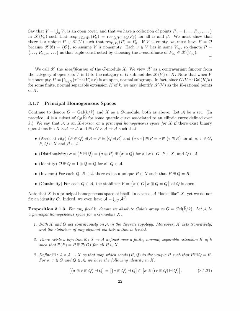
It suffices then to show that (Associativity) holds for ⊕ : X ×X → X. For this, it suffices toshow that
(P ⊕Q
)∗R = P ∗
(Q⊕R
)for all P, Q, R ∈ X. We omit a rigorous proof, and instead
give a geometric one for k ⊆ R. See Figure 3.1.
3.1.4 Tate Modules
Let X and Y be G-modules, and say that we have a G-module homomorphism f : X → Y . Wesay that f is an isogeny if either f(P ) = O for all P ∈ X or f has the following properties:
• (Homomorphism) f(P ⊕Q) = ϕ(P )⊕ ϕ(Q) for all P, Q ∈ X.
• (G-Map) σ } f(P ) = f(σ } P ) for all σ ∈ G and P ∈ X.
• (Kernel) The kernel X[f ] ={P ∈ X
∣∣ f(P ) = O}
is a finite group.
• (Image) The image f(X) = Y . That is, for each Q ∈ Y , there exists at least one P ∈ X suchthat f(P ) = Q.
If f : X → Y is an isogeny, define the (separable) degree as the integer deg f = #X[f ].
For each integer m, define the “multiplication-by-m” map [m] : X → X as that map whichsends
[m]P =
P ⊕ · · · ⊕ P︸ ︷︷ ︸m times
if m > 0;
(−P )⊕ · · · ⊕ (−P )︸ ︷︷ ︸|m| times
if m < 0; and
O if m = 0.
(3.1.6)
This is a G-module homomorphism. Let m = `α be a power of a prime `; then X[`α] is a G-submodule of X. We have projection maps
projβ,α : X[`β]→ X[`α] which sends P 7→ [`β−α]P (3.1.7)
17

-4.8
-4.4
-4-3.6
-3.2
-2.8
-2.4
-2-1.6
-1.2
-0.8
-0.4
00.4
0.8
1.2
1.6
22.4
2.8
3.2
3.6
44.4
4.8
-3
-2.5
-2
-1.5
-1
-0.5
0.51
1.52
2.53
P
R
P*Q
P+
Q
Q*R
(P+
Q)*
R =
P*(Q
+R)
Q+
R
Q
Figure 3.1: A Geometric Proof of the Associativity of the Group Law18

whenever α ≤ β. We define the `-adic Tate module for X as the projective limit
T`(X) = lim←−α
X[`α] =
{(. . . , Pα, . . . ) ∈
∏α∈I
X[`α]
∣∣∣∣∣ [`β−α]Pβ = Pα
}(3.1.8)
This is a Z`[G]-module. To see why, define } : Z`[G]× T`(X)→ T`(X) by[∑σ∈G
m(σ)σ
]} P =
(. . . ,
∑σ∈G
σ } [mα(σ)]Pα, . . .
). (3.1.9)
Each mα ∈ Z/`α Z. If mα = nα + aα `α, then
[mα]Pα = [nα]Pα ⊕ [aα]([`α]Pα
)= [nα]Pα ⊕O = [nα]Pα. (3.1.10)
Define V`(X) = T`(X) ⊗Z` Q` as a Q`-module. Since G acts continuously on V`(X), we have acontinuous representation
ρX,` : Gal(k/k
)→ GL
(V`(X)
). (3.1.11)
We define this as the `-adic representation associated to X.
3.1.5 Isogenies of Galois Modules
Let X, Y , and Z be G-modules.
• Say that we haveG-module homomorphisms f : X → Y and h : X → Z. Wheneverker f ⊆ kerh and im f = Y , there exists a G-module homomorphism g : Y → Zwhich makes the following diagram commute:
X
f
��
h // Z
Y
g
?? (3.1.12)
• Let f : X → Y be an isogeny, and denote m = deg f as its (separable) degree.There exists a G-module homomorphism f : Y → X such that f ◦ f = [m] is the“multiplication-by-m” map.
Proof. Write ϕ−1(Q) = R ⊕ f−1(O) for some R ∈ f−1(Q); then #f−1(Q) = #f−1(O) = m. Forthe composition f ◦ f : X → X we have(
f ◦ f)(P ) =
⊕R∈f−1
(f(P )
)R =⊕
R∈f−1(O)
f(P ) = (3.1.13)
For the composition f ◦ f : Y → Y we have
(f ◦ f
)(Q) = ϕ
⊕R∈f−1(Q)
R
=⊕
R∈f−1(Q)
ϕ(R) =⊕
R∈f−1(Q)
Q = [m]Q. (3.1.14)
Hence f ◦ f = [m] is indeed the “multiplication-by-m” map.
19

3.1.6 Sheaves of Galois Modules
Continue to denote G = Gal(k/k
)and X as a G-module, both as above. Given any element ν ∈ G,
define the subset
Xν =⋃ν∈V
{P ∈ X
∣∣σ } P = P for all σ ∈ V}
(3.1.15)
as the union over those open subsets V ⊆ G containing ν. We call Xν the stalk over ν, andany element Pν ∈ Xν a germ of the stalk. Given any nonempty open set V ⊆ G, define UV =⋂τ∈G
(τ−1 ◦ 〈V 〉 ◦ τ
)as the largest normal, open subgroup contained in the group generated by V ;
for V being empty, define U∅ = G. We wish to consider the subset
X (V ) =
(. . . , Pν , . . . ) ∈∏ν∈V
Xν
∣∣∣∣∣∣∣for each ν ∈ V , there exists a normal,
open subgroup Uν ⊆ G such that ν ◦ Uν ⊆ Vand σ } Pν◦ω = Pν◦ω for all σ ∈ UV and ω ∈ Uν
,
(3.1.16)where we set X (∅) = {O}. We may identify each point P =
(. . . , Pν , . . .
)in X (V ) as a morphism
P : V →⋃ν∈V
Xν defined by ν 7→ Pν . (3.1.17)
Proposition 3.1.2. For any field k, denote its absolute Galois group as G = Gal(k/k
). Let X be
a G-module, Xν ⊆ X be a stalk for each ν ∈ G, and X (V ) as above for each open set V ⊆ G.
1. Xν is a G-module.
2. X is a sheaf of G-modules.
Proof. We begin by showing that each stalk Xν is a G-module. Since Xν =⋂ν∈U X
U is theintersection over normal, open subgroups U containing ν, it suffices to show that each XU is aG-module. First, we show that there are restrictions ⊕ : XU ×XU → XU and } : G×XU → XU .Each subset XU is closed under addition because σ}
(P ⊕Q
)=(σ}P
)⊕(σ}Q
)= P ⊕Q for any
σ ∈ U and P, Q ∈ XU . As U is a normal subgroup in G, the conjugate σ′ = τ−1 ◦σ ◦ τ is also in Ufor any τ ∈ G. Hence σ}
(τ }P
)= τ }
(σ′}P
)= τ }P , showing that τ }P is also in XU for any
τ ∈ G. Hence properties (Associativity), (Commutativity), (Distributivity), and (Continuity) hold.Property (Identity) holds because
(σ}O
)⊕(σ}O
)= σ}
(O⊕O
)= σ}O, so that σ}O = O for
any σ ∈ G. Property (Inverses) holds because(σ}P
)⊕(σ}(−P )
)= σ}
(P⊕(−P )
)= σ}O = O,
so that σ } (−P ) = −(σ } P
)for any σ ∈ G. In particular, σ } (−P ) = −P for any σ ∈ U and
P ∈ XU .
Proposition 2.2.1 shows that G is a topological space. In order to show that X is a sheaf, wemust show that the following three properties hold:
• (G-Modules) X (V ) is a G-module for every open set V ⊆ G, where X (∅) = {O}.
We define binary operations ⊕ : X (V )×X (V )→X (V ) and } : G×X (V )→X (V ) component-wise:
P =(. . . , Pν , . . .
)Q =
(. . . , Qν , . . .
)}
=⇒
{P ⊕Q =
(. . . , Pν ⊕Qν , . . .
)τ } P =
(. . . , τ } Pν , . . .
) (3.1.18)
20

We explain why these are well-defined. Fix P, Q ∈X (V ). For each ν ∈ V , we can find normal, opensubgroups Uν,P , Uν,Q ⊆ G such that ν◦Uν,P , ν◦Uν,Q ⊆ V and σ}Pν◦ω = Pν◦ω, σ}Qν◦ω′ = Qν◦ω′ forall σ ∈ UV and ω ∈ Uν,P , ω′ ∈ Uν,Q. (Recall that for V nonempty we set UV =
⋂τ∈G
(τ−1 ◦〈V 〉◦τ
),
and U∅ = G otherwise.) Define Uν = Uν,P ∩ Uν,Q; this is a normal, open subgroup such thatν ◦ Uν ⊆ V . Property (Distributivity) for the stalks Xν◦ω implies that σ }
(Pν◦ω ⊕ Qν◦ω
)=(
σ } Pν◦ω)⊕(σ } Qν◦ω
)= Pν◦ω ⊕ Qν◦ω for all σ ∈ UV and ω ∈ Uν , showing that P ⊕ Q is in
X (V ). As UV is a normal subgroup, the conjugate σ′ = τ−1 ◦ σ ◦ τ is also in UV for any τ ∈ G.Then σ }
(τ } Pν◦ω
)= τ }
(σ′ } Pν◦ω
)= τ } Pν◦ω for all σ ∈ UV and ω ∈ Uν , showing that τ } P
is in X (V ).It is easy to see that properties (Associativity), (Commutativity), and (Distributivity) hold.
As σ } O = O and σ } (−Pν) = −(σ } Pν
)for all σ ∈ G, the elements O =
(. . . , O, . . .
)and
−P =(. . . , −Pν , . . .
)are in X (V ); hence properties (Identity) and (Inverses) hold. It remains
to show that property (Continuity) holds. Fix a point P =(. . . , Pν , . . .
)in X (V ), and consider
an element σ of the stabilizer{σ ∈ G
∣∣σ } P = P}
=⋂ν∈V
{σ ∈ G
∣∣σ } Pν = Pν}
. This groupcontains the open set σ ◦UV , so that it is indeed open. Hence X (V ) is a G-module for every openset V ⊆ G.
• (Restriction Morphisms) Whenever we have open sets U ⊆ V ⊆ W , there exist G-modulehomomorphisms
resW/U : X (W )resW/V−−−−→ X (V )
resV/U−−−−→ X (U) (3.1.19)
such that resV/V = 1.
Define the map resW/V : X (W )→X (V ) as that which takes a tuple P =(. . . , Pν , . . .
)for ν ∈W
to that tuple resW/V (P ) =(. . . , Pν , . . .
)for ν ∈ V which is formed by removing those coordinates
corresponding to ν ∈W −V . We explain why this is well-defined for V nonempty. For each ν ∈W ,there exists a normal, open subgroup U ′ν ⊆ G such that ν ◦ U ′ν ⊆ W and σ } Pν◦ω = Pν◦ω forall σ ∈ UW and ω ∈ U ′ν . As V is open, we can find a normal, open subgroup U ′′ν ⊆ G such thatν ◦ U ′′ν ⊆ V . Denote Uν = U ′ν ∩ U ′′ν ; this is a normal, open subgroup such that ν ◦ Uν ⊆ V . AsV ⊆W , we have UV ⊆ UW – recall that V is assumed nonempty – so that σ } Pν◦ω = Pν◦ω for allσ ∈ UV and ω ∈ Uν . This shows that resW/V (P ) is indeed in X (V ).
As σ } O = O, it is clear that σ }[resW/V (P )
]= resW/V
[σ } P
]and resW/V
(P ⊕ Q
)=
resW/V (P )⊕ resW/V (Q) for all σ ∈ G and P, Q ∈ X (W ); hence resW/V is a G-module homomor-phism. Similarly, it is clear that resW/U = resV/U ◦ resW/V and resV/V = 1 whenever U ⊆ V ⊆W .
• (Gluing Property) Say that V =⋃α Vα is a covering of open sets. Whenever we have a
collection of points Pα ∈ X (Vα) such that resVα/Vα∩Vβ (Pα) = resVβ/Vα∩Vβ (Pβ) for all α andβ, then there exists a unique P ∈X (V ) such that resV/Vα(P ) = Pα.
V P.resV/Vα
ww
�resV/Vβ
''Vα+ �
88
Vβ3 S
ff
Pα �
''
Pβ/
wwVα ∩ Vβ3 S
ee
+ �
99
resV/Vα∩Vβ (P )
(3.1.20)
21
Say that V =⋃α Vα is an open cover, and that we have a collection of points Pα =
(. . . , Pα,ν , . . .
)in X (Vα) such that resVα/Vα∩Vβ (Pα) = resVβ/Vα∩Vβ (Pβ) for all α and β. We must show thatthere is a unique P ∈ X (V ) such that resV/Vα(P ) = Pα. If V is empty, we must have P = Obecause X (∅) = {O}, so assume V is nonempty. Each ν ∈ V lies in some Vαν , so denote P =(. . . , Pαν ,ν , . . .
)as that tuple constructed by choosing the ν-coordinate of Pαν ∈X (Vαν ).
We call X the sheafification of the G-module X. We view X as a contravariant functor fromthe category of open sets V in G to the category of G-submodules X (V ) of X. Note that when Vis nonempty, U =
⋂τ∈G
(τ−1◦〈V 〉◦τ
)is an open, normal subgroup. In fact, since G/U ' Gal(K/k)
for some finite, normal separable extension K of k, we may identify X (V ) as the K-rational pointsof X.
3.1.7 Principal Homogeneous Spaces
Continue to denote G = Gal(k/k
)and X as a G-module, both as above. Let A be a set. (In
practice, A is a subset of Cd(k) for some quartic curve associated to an elliptic curve defined overk.) We say that A is an X-torsor or a principal homogeneous space for X if there exist binaryoperations � : X ×A → A and � : G×A → A such that
• (Associativity)(P ⊕Q
)�R = P �
(Q�R
)and
(σ ◦ τ
)�R = σ �
(τ �R
)for all σ, τ ∈ G,
P, Q ∈ X and R ∈ A.
• (Distributivity) σ �(P �Q
)=(σ } P
)�(σ �Q
)for all σ ∈ G, P ∈ X, and Q ∈ A.
• (Identity) O �Q = 1 �Q = Q for all Q ∈ A.
• (Inverses) For each Q, R ∈ A there exists a unique P ∈ X such that P �Q = R.
• (Continuity) For each Q ∈ A, the stabilizer V ={σ ∈ G
∣∣σ �Q = Q}
of Q is open.
Note that X is a principal homogeneous space of itself. In a sense, A “looks like” X, yet we do notfix an identity O. Indeed, we even have A =
⋃U AU .
Proposition 3.1.3. For any field k, denote its absolute Galois group as G = Gal(k/k
). Let A be
a principal homogeneous space for a G-module X.
1. Both X and G act continuously on A in the discrete topology. Moreover, X acts transitively,and the stabilizer of any element via this action is trivial.
2. There exists a bijection Ξ : X → A defined over a finite, normal, separable extension K of ksuch that Ξ(P ) = P � Ξ(O) for all P ∈ X.
3. Define � : A×A → X as that map which sends (R,Q) to the unique P such that P �Q = R.For σ, τ ∈ G and Q ∈ A, we have the following identity in X:[(
σ � τ �Q)�Q
]=[(σ �Q
)�Q
]⊕[σ }
((τ �Q)�Q
)]. (3.1.21)
22

4. Define the relation A ∼ B when B is a principal homogeneous space for X and there is abijection f : A → B, commuting with the action by G, satisfying f(P � Q) = P � f(Q) forall P ∈ X and Q ∈ A. Then ∼ is an equivalence relation. Moreover, for σ ∈ G, Q ∈ A, andR ∈ B, we have the following identity in X:[(
σ �Q)�Q
]=[(σ �R
)�R
]⊕[(σ } P
)⊕ (−P )
](3.1.22)
where P = f(Q)�R is in X.
Three principal homogeneous spaces A, B, and C for a G-module X are said to be equivalentwhen we can find maps f : A → B and g : B → C which make the following diagram commute:
X∼−−−−→ X
∼−−−−→ X
ΞA
y ΞB
y ΞC
yA f−−−−→ B g−−−−→ C
(3.1.23)
In fact, it is easy to verify that top row is a translation map P 7→ P ⊕ OB,A 7→ P ⊕ OC,A for all
P ∈ X, in terms of OB,A =(ΞB−1 ◦ f ◦ ΞA
)(O), etc. (Milne, in his “Etale Cohomology”, denotes
PSH(X/k) as the set of equivalence classes {A/X} of such principal homogeneous spaces for X.)
Proof. The action of X on A is Q 7→ P �Q for any fixed P ∈ X. As(X, ⊕
)is an abelian group
with identity O, properties (Associativity) and (Identity) show that both X and G do indeed acton A. Property (Inverses) shows that the only P = O if the only element such that P � Q = Q;hence the stabilizer of any Q ∈ A is the trivial group {O} ⊆ X. As one point sets are open inthe discrete topology, this shows that the group action is continuous. Similarly, property (Inverses)shows that any R ∈ A is in the orbit of a given Q ∈ A, so this action is transitive.
Fix Q ∈ A. Define Ξ : X → A by Ξ(P ) = P � Q. Clearly this is well-defined and bijective.Let V be the stabilizer of Q. As G acts on A continuously, we can find an open normal subgroupU ⊆ V ⊆ G, so that G/U ' Gal(K/k) for some finite, normal, separable extension K of k. Clearly,Ξ is defined over K.
Continue to fix Q ∈ A. For each σ ∈ G, denote ξ(σ) =(σ � Q
)� Q as that unique element
such that ξ(σ) � Q = σ � Q. It suffices to show that ξ(σ ◦ τ) = ξ(σ) ⊕(σ } ξ(τ)
). We have the
identity
ξ(σ ◦ τ)�Q =(σ ◦ τ
)�Q = σ �
(τ �Q
)= σ �
(ξ(τ)�Q
)=(σ } ξ(τ)
)�(σ �Q
)=[(σ } ξ(τ)
)⊕ ξ(σ)
]�Q,
(3.1.24)
where we have used properties (Associativity) and (Distributivity). As ξ(σ) is unique, we musthave ξ(σ ◦ τ) = ξ(σ)⊕
(σ } ξ(τ)
)as desired.
We show that ∼ is an equivalence relation. Clearly A ∼ A since we may choose f = 1. Assumethat A ∼ B. Denote f−1 : B → A as the inverse of the map f : B → A. Choose P ∈ A and R ∈ B,and denote Q = f−1(R) ∈ A. Then we have
f−1(P �R
)= f−1
(P � f(Q)
)= f−1
(f(P �Q)
)= P �Q = P � f−1(R). (3.1.25)
Hence B ∼ A. Now assume that A ∼ B and B ∼ C. Denote f : A → B and g : B → C as bijectionssuch that for all P ∈ X, Q ∈ A, and R ∈ B we have f(P�Q) = P�f(Q) and g(P�R) = P�g(R).The composition h = g ◦ f : A → C is also a bijection. We have the identity
h(P �Q) = g(f(P �Q)
)= g(P � f(Q)
)= P �
(g ◦ f(P )
)= P � h(Q). (3.1.26)
23
Hence A ∼ C. This shows that ∼ is indeed an equivalence relation. Fix σ ∈ G, Q ∈ A, andR ∈ B. Define ξA(σ), ξB(σ), P ∈ X via the relations ξA(σ)�Q = σ �Q, ξB(σ)�R = σ �R, andP �R = f(Q). We have the identity
(ξA(σ)⊕ P
)� f(Q) = P �
[ξA(σ)� f(Q)
]= P �
[f(ξA(σ)�Q
)]= P � f
(σ �Q
)= P �
(σ � f(Q)
)= P �
(σ �
[P �R
])= P �
(σ } P
)�(σ �R
)= P �
(σ } P )�
(ξB(σ)�R
)=(ξB(σ)⊕
(σ } P
))�(P �R
)=(ξB(σ)⊕
(σ } P
))� f(Q).
(3.1.27)
This shows that ξA(σ)⊕ P = ξB(σ)⊕(σ ◦ P
), so that ξA(σ) = ξB(σ)⊕
[(σ } P )⊕ (−P )
].
3.1.8 Torsors via Translation Maps
If A is a principal homogeneous space for X, then there exists a bijection Ξ : X → A. The followingresult gives a partial converse: if there exists a certain type of bijection Ξ : X → A, then there isa binary operation � : X ×A → A such that A is a principal homogeneous space for X.
Proposition 3.1.4. For any field k, denote its absolute Galois group as G = Gal(k/k
). Let X
and Y be G-modules, f : X → Y be a G-module homomorphism, and A and B be sets on which Gacts continuously. Assume that we have bijections ΞA : X → A and ΞB : Y → B such that for eachσ ∈ G there exists ξB(σ) = f
(ξA(σ)
)∈ Y for ξA(σ) ∈ X satisfying
σ � ΞA(P ) = ΞA((σ } P )⊕ ξA(σ)
)σ � ΞB(Q) = ΞB
((σ }Q)⊕ ξB(σ)
) for allP ∈ X,
Q ∈ Y.(3.1.28)
1. The map � : X × A → A defined by P � Q = ΞA(P ⊕ Ξ−1
A (Q))
makes A a principalhomogeneous space for X. Moreover, ΞA(P ) = P � ΞA(O) for all P ∈ X.
2. Then there is a map f∗ : A → B such that f∗(P�Q) = f(P )⊕f∗(Q) and σ}f∗(Q) = f∗(σ�Q)for all σ ∈ G, P ∈ X, and Q ∈ A. Moreover, the following diagram commutes:
GξA
uu
ξB
))X
ΞA��
f // Y
ΞB��
A f∗ // B
(3.1.29)
This proposition explains how the existence of a bijection ΞA : X → A which depends on a mapξA : G→ X constructs homogeneous spaces. We say that A is an f -descendant of B whenever theconditions above hold. Note that if ξB = O, then B ' Y as G-modules and im ξA ⊆ ker f . In thiscase, we say A an f -cover for Y , with f∗ : A → Y being the covering map.
Proof. We show that � : X ×A → A satisfies the following properties:
• (Associativity)(P ⊕Q
)�R = P �
(Q�R
)for all P, Q ∈ X and R ∈ A.
24
• (Distributivity) σ �(P �Q
)=(σ } P
)�(σ �Q
)for all σ ∈ G, P ∈ X, and Q ∈ A.
• (Identity) O �Q = Q for all Q ∈ A.
• (Inverses) For each Q, R ∈ A there exists a unique P ∈ X such that P �Q = R.
• (Translation) ΞA(P ) = P � ΞA(O) for all P ∈ X.
For (Associativity), we have(P ⊕Q
)�R = ΞA
(P ⊕Q⊕Ξ−1
A (R))
= ΞA(P ⊕Ξ−1
A[ΞA(Q⊕Ξ−1
A (R))])
= P �(Q�R
). (3.1.30)
For (Distributivity),
σ �(P �Q
)= σ � ΞA
(P ⊕ Ξ−1
A (Q))
= f((σ } P )⊕
[σ } Ξ−1
A (Q)]⊕ ξA(σ)
)= ΞA
((σ } P )⊕
[σ } Ξ−1
A (Q)⊕ ξ(σ)])
= ΞA((σ } P )⊕ Ξ−1
A[σ �Q
])=(σ } P
)�(σ �Q
).
(3.1.31)
For (Identity), we have O � Q = ΞA(O ⊕ Ξ−1
A (Q))
= ΞA(Ξ−1A (Q)
)= Q. For (Inverses), let
Q, R ∈ A be given, and define P = Ξ−1A (R) ⊕
(−Ξ−1A (Q)
). It is easy to see that P ∈ X is
that unique element such that P � Q = R. For (Translation), let Q = ΞA(O). Then ΞA(P ) =ΞA(P ⊕O
)= ΞA
(P ⊕ Ξ−1
A (Q))
= P �Q = P � ΞA(O).Define f∗ : A → B by the composition f∗ = ΞB ◦ f ◦ΞA
−1. For any P ∈ X and Q ∈ A, we have
f∗(P �Q
)= ΞB ◦ f
(P ⊕ ΞA
−1(Q))
= ΞB
[f(P )⊕
(f ◦ ΞA
−1)(Q)
]= f(P )⊕ f∗(Q). (3.1.32)
Now choose σ ∈ G and Q ∈ A, and set P = ΞA−1(Q). Since σ � Q = ΞA
((σ } P ) ⊕ ξA(σ)
), we
have
f∗(σ �Q) = ΞB ◦ f((σ } P )⊕ ξA(σ)
)= ΞB
[f(σ } P
)⊕ f
(ξA(σ)
)]= ΞB
[(σ } f(P )
)⊕ ξB(σ)
]= σ � ΞB
(f(P )
)= σ � f∗(Q).
(3.1.33)
By construction, the diagram commutes.
3.1.9 Example: Quadratic Curves
The following proposition explains how to determine conic sections as principal homogeneous spacesfor Pell’s equation x2 −Dy2 = 1.
Proposition 3.1.5. Let k be a field of characteristic different from 2, and denote its absoluteGalois group as G = Gal
(k/k
). Fix elements ai ∈ k such that the determinants
a11, D = −∣∣∣∣a11 a12
a12 a22
∣∣∣∣ and
∣∣∣∣∣∣a11 a12 a13
a12 a22 a23
a13 a23 a33
∣∣∣∣∣∣ (3.1.34)
are nonzero.
25

1. Denote X as the collection of k-rational points P = (x, y) satisfying x2 −Dy2 = 1. Then Xis a G-module via the binary operation ⊕ : X ×X → X defined by
(x1, y1)⊕ (x2, y2) =(x1 x2 +Dy1 y2, x1 y2 + x2 y1
). (3.1.35)
2. Denote A as the collection of k-rational points Q = (z, w) on the conic section
a11 z2 + 2 a12 z w + a22w
2 + 2 a13 z + 2 a23w + a33 = 0. (3.1.36)
Then A is a principal homogeneous space for X.
Proof. Consider the injective group homomorphism
X → SL2(k) defined by (x, y) 7→[x D yy x
]. (3.1.37)
(The obvious map X → k×
defined by P 7→ x +√Dy is a homomorphism of G-modules, but it
is not injective!) As SL2(k) is G-module, the induced structure turns X into a G-module as well.Note that (x, y) ⊕ (−1, 0) = (−x,−y), while O = (1, 0) is the identity and −P = (x,−y) is theinverse.
Consider the bijection Ξ : X → A defined by
Ξ(x, y) =
(z0 +
x− a12 y√d
, w0 +a11 y√d
)where Ξ(O) =
(z0 +
1√d, w0
) in terms of
z0 =
a12 a23 − a13 a22
a11 a22 − a212
,
w0 =a12 a13 − a11 a23
a11 a22 − a212
.
(3.1.38)This is defined over the finite, normal, separable extension K = k(
√d) of k, where
d = −a11
∣∣∣∣a11 a12
a12 a22
∣∣∣∣∣∣∣∣∣∣a11 a12 a13
a12 a22 a23
a13 a23 a33
∣∣∣∣∣∣−1
= − a11
a13 z0 + a23w0 + a33. (3.1.39)
Geometrically, the point Q0 = (z0, w0) is the “center” of the conic section; it is not actually on thecurve. It is easy to check that
σ[Ξ(P )
]= Ξ
((σ P )⊕ ξ(σ)
)where ξ(σ) =
{(−1, 0) if σ(
√d) = −
√d;
O if σ(√d) = +
√d.
(3.1.40)
Proposition 3.1.4 states that A is a principal homogeneous space for X. For example, the binaryoperation � : X ×A → A defined by
(x, y)� (z, w) = f((x, y)⊕ f−1(z, w)
)=
(z0 + x (z − z0)− y (a12 z + a22w + a23), w0 + x (w − w0) + y (a11 z + a12w + a13)
)(3.1.41)
26
which may also be realized via the injective group homomorphism
Y → SL2(k) defined by (z, w) 7→
a11 z + a12w + a13a12 z + a22w + a23
a13 z0 + a23w0 + a33
w − w0 − z − z0
a13 z0 + a23w0 + a33
.(3.1.42)
The proposition follows.
3.1.10 Example: Cubic Curves
3.2 Selmer’s Cubic
Proposition 3.2.1. Let k be a field of characteristic different from 2 and 3. Fix D ∈ k×, andconsider the cubic curve C : a u3 + b v3 + cw3 = 0 for a, b, c ∈ k satisfying D = a b c.
1. C is a principal homogeneous space for the elliptic curve E : y2 = x3−432D2. In particular,E acts continuously and transitively on C via the map � : E × C → C given by
(x, y)� (u : v : w)
=
(2w y + (x2 − 17) z
(x2 + 17) + 34x z2,w[x4 − 172
]− 34 z
[xw z (x2 − 17) + y (2x+ 17 z2 + x2 z2)
][(x2 + 17) + 34x z2
]2).
(3.2.1)
2. Denoting the elliptic curve E′ : y2 = x3 + 27D2 x, there are rational maps ϕ′ : E → E′ andg : C → E′ defined over k which make the following diagram commute:
E
f
��
ϕ′ // E′
C
g
>> (3.2.2)
Moreover, g(P �Q) = ϕ′(P )⊕ g(Q) for all P on E and Q on C.
3. If C has a k-rational point Q0 = (u0 : v0 : w0), then C and E are birationally equivalent overk.
Ernst Selmer considered this family of cubic curves for k = Q. In particular, he showed thatC : 3u3 + 4 v3 + 5w3 = 0 has a Qv-rational point for every place v of Q, yet it has no Q-rationalpoint. We will see later that we can use properties of the Selmer group to better understand thisphenomenon.
Proof. Denote X = E(k) as the collection of k-rational points P = (x, y) on the cubic curveE : y2 = x3 − 432D2. As its discriminant is a nonzero ∆ = −212 · 39 · D4, we see that E is anelliptic curve defined over k. Recall that X is a G-module by Proposition 3.1.1. Denote Y = C(k)as the collection of k-rational points Q = (u, v, w) the quartic curve C : a u3 + b v3 + cw3 = 0. Themap f : E → C defined by
f(x, y) =
(−6 b x
3√d
:36 a b c− y
3√d2
:36 a b c+ y
d
)where f(O) =
(0 :
3√d : 1) (3.2.3)
27

is a bijection from X to Y which is defined over the finite, normal, separable extension K =k(√−3, 3√d) of k for d = c/b. Using the identity (x, y) ⊕ (0, 0) =
(17/x, −17 y/x2
)for the group
law on E, one checks that for any σ in G = Gal(k/k
)we have the relation
σ[f(P )
]= f
((σ P )⊕ ξ(σ)
)where ξ(σ) =
{(0, 0) if σ(
√2) = −
√2;
O if σ(√
2) = +√
2.(3.2.4)
Proposition 3.1.4 states that Y = C(k) is a principal homogeneous space for X = E(k). The map� : X × Y → Y above is defined by (x, y)� (u : v : w) = f
((x, y)⊕ f−1(u : v : w)
).
We have seen before that there is a 2-isogeny ϕ′ : E → E′ defined by
ϕ′(x, y) =
(x2 + 17
x, y
x2 − 17
x2
)=⇒
(ϕ′ ◦ f−1
)(z, w) =
(2
z2,
4w
z3
). (3.2.5)
Since im ξ ={
(0, 0), O}
= E[ϕ′], the second statement in the proposition above follows fromProposition 3.1.4.
Finally, say that Q0 = (u0 : v0 : w0) is a k-rational point on C. Since
x =1− 17 z2 z2
0 + 2ww0
(z − z0)2
y =34 z z0 (z2w0 + z2
0 w)− 2 (w + w0)
(z − z0)3
(3.2.6)
if and only if
z = z0 + 2−w0 y + 17 z3
0 x+ 17 z0
x2 + 34 z20 x+ 17
w = w0 − 34z0
(z2
0 x2 + 2x+ 17 z2
0
)y + w0
(3 z2
0 x3 + 34 z4
0 x2 + x2 + 17z2
0 x+ 17)(
x2 + 34 z20 x+ 17
)2(3.2.7)
we see that the quartic curve 2w2 = 1 − 17 z4 is birationally equivalent over k to the cubic curvey2 = x3 + 17x.
Proposition. Let k be a field of characteristic different from 3 containing a cube rootζ3 of unity. (In practice, we choose k = Q(
√−3) since we want a number field.) Choose
k-rational numbers A, B, C, and D such that ∆ = 27ABC(D3 −ABC
)3is nonzero.
We want to consider the projective curves
C : Az31 +B z3
2 + C z30 = 3D z1 z2 z0.
These are called Desboves’ Curves. An example would be 3 z31 + 4 z3
2 + 5 z30 = 0. This
family of curves has complex multiplication, i.e., for a primitive cube root ζ3 of unity,we have an automorphism of order 3 defined by
[ζ3] : C(k)→ C(k) which sends(z1 : z2 : z0
)7→(ζ3 z1 : ζ2
3 z2 : z0
). (3.2.8)
28
First, we show why this is a principal homogeneous space for an elliptic curve. Consider themap f : E → C defined by
f(x, y) =
(3B x
3√d
:3Dx+ (1− ζ3) y + (1− ζ2
3 ) (D3 −ABC)3√d2
:3Dx+ (1− ζ2
3 ) y + (1− ζ3) (D3 −ABC)
d
)where f(O) =
(0 :
3√d : −1
)(3.2.9)
for the elliptic curve E : y2 + 3Dxy + (D3 − ABC) y = x3 and d = C/B. This is defined overthe finite, normal, separable extension K = k( 3
√d) of k, and one checks that
σ[f(P )
]= f
((σ P )⊕ ξ(σ)
)where ξ(σ) =
(0, 0) if σ( 3
√d) = ζ3
3√d;
(0,−b) if σ( 3√d) = ζ2
33√d;
O if σ( 3√d) = 3
√d.
(3.2.10)
Hence C is indeed a principal homogeneous space for E.Second, we show that if C has a rational point P0 =
(a1 : a2 : a0
), then C is birationally
equivalent to a different elliptic curve.
3.2.1 Example: Quartic Curves
The following proposition explains how to determine quartic curves as principal homogeneous spacesfor elliptic curves.
Proposition 3.2.2. Let k be a field of characteristic different from 2, and denote its absoluteGalois group as G = Gal
(k/k
). Consider a quartic Q(z) = c4 z
4 + c3 z3 + c2 z
2 + c1 z + c0 withcoefficients in k and a nonzero discriminant
Disc(Q) = c21 c
22 c
23 − 4 c0 c
32 c
23 − 4 c3
1 c33 + 18 c0 c1 c2 c
33 − 27 c2
0 c43 − 4 c2
1 c32 c4
+ 16 c0 c42 c4 + 18 c3
1 c2 c3 c4 − 80 c0 c1 c22 c3 c4 − 6 c0 c
21 c
23 c4 + 144 c2
0 c2 c23 c4
− 27 c41 c
24 + 144 c0 c
21 c2 c
24 − 128 c2
0 c22 c
24 − 192 c2
0 c1 c3 c24 + 256 c3
0 c34.
(3.2.11)
Define the coefficients
a1 =c3
3 − 4 c2 c3 c4 + 8 c1 c24
8 c24
a2 =3 c2
3 − 8 c2 c4
4 c4
a4 =3 c4
3 − 16 c2 c23 c4 + 16 c2
2 c24 + 16 c1 c3 c
24 − 64 c0 c
34
16 c24
a6 =
(c3
3 − 4 c2 c3 c4 + 8 c1 c24
)264 c3
4
(3.2.12)
1. The polynomial P (x) = x3 + a2 x2 + a4 x+ a6 in terms of is a resolvent cubic for Q(z) such
that Disc(P ) = Disc(Q).
2. The quartic curve C : w2 = Q(z) is a principal homogeneous space for the elliptic curveE : y2 = P (x). If C has a k-rational point Q0 = (z0, w0), then C and E are birationallyequivalent over k.
29

3. Assume that a1 = 0.
In particular, the quartic curves w2 = 1 − z4 and 2w2 = 1 − 17 z4 are principal homogeneousspaces for the cubic curves y2 = x3 + 4x and y2 = x3 + 17x, respectively, as well as g-covers forthe cubic curves y2 = x3 − x and y2 = x3 − 68x, respectively. We will see later that the formerquartic curve has Q-rational points, whereas the latter quartic curve does not.
Proof. Using the factorization Q(z) = c4 (z − e1) (z − e2) (z − e3) (z − e4) over k, we find thefactorization
P (x) =
[x+ c4
(e1 + e2 − e3 − e4)2
4
] [x+ c4
(e1 − e2 + e3 − e4)2
4
] [x+ c4
(e1 − e2 − e3 + e4)2
4
](3.2.13)
also over k. One readily verifies that Disc(P ) = Disc(Q).Denote X = E(k) as the collection of k-rational points P = (x, y) satisfying y2 = P (x), and
A = C(k) as the collection of k-rational points Q = (z, w) satisfying w2 = Q(z). The discriminantof the cubic curve is ∆ = 24 · Disc(Q). As this is nonzero, we see that E is indeed an ellipticcurve over k; Proposition 3.1.1 states that X is indeed a G-module. The birational transformationΞ : X → A defined by
Ξ(x, y) =
(−c3 x+ 2 c4 a1 + 2 d y
4 c4 x,d(2 a6 + a4 x− x3
)+2 c4 a1 y
4 c4 x2
)(3.2.14)
is defined over the finite, normal, separable extension K = k(√d) of k, where d = c4. It is easy to
check that
σ[Ξ(P )
]= Ξ
((σ P )⊕ ξ(σ)
)where ξ(σ) =
(
0, a1
√d)
if σ(√d) = −
√d;
O if σ(√d) = +
√d.
(3.2.15)
Proposition 3.1.4 states that A is a principal homogeneous space for X.Say that Q0 = (z0, w0) is a k-rational point on C. Then the invertible substitution
x =b1 (z − z0) + b2
z − z0+
b3(z − z0
)2 (w − w0)
y =b4 (z − z0)2 + b5 (z − z0) + b6(
z − z0
)2 +b7 (z − z0) + b8(
z − z0
)3 (w − w0)
(3.2.16)
in terms of the coefficients
b1 = 2 c4 z20 + c3 z0
b2 = 4 c4 z30 + 3 c3 z
20 + 2 c2 z0 + c1
b3 = −2w0
b4 = w0
(4 c4 z0 + c3
)b5 = 2w0
(6 c4 z
20 + 3 c3 z0 + c2
)b6 = 2w0
(4 c4 z
30 + 3 c3 z
20 + 2 c2 z0 + c1
)b7 = −
(4 c4 z
30 + 3 c3 z
20 + 2 c2 z0 + c1
)b8 = −4w2
0
(3.2.17)
shows that the relation y2 = P (x) holds if and only if w2 = Q(z) holds. Hence the curves C and Eare birationally equivalent over k.
30

Proposition 3.2.3. Let k be a field of characteristic different from 2, and denote its absoluteGalois group as G = Gal
(k/k
). Fix ci ∈ k such that the discriminants
c4 6= 0,
c33 − 4 c2 c3 c4 + 8 c1 c
24 = 0,
c21 c
22 c
23 − 4 c0 c
32 c
23 − 4 c3
1 c33 + 18 c0 c1 c2 c
33 − 27 c2
0 c43 − 4 c2
1 c32 c4
+ 16 c0 c42 c4 + 18 c3
1 c2 c3 c4 − 80 c0 c1 c22 c3 c4 − 6 c0 c
21 c
23 c4 + 144 c2
0 c2 c23 c4
− 27 c41 c
24 + 144 c0 c
21 c2 c
24 − 128 c2
0 c22 c
24 − 192 c2
0 c1 c3 c24 + 256 c3
0 c34 6= 0.
(3.2.18)
1.
C : w2 = c4 z4 + c3 z
3 + c2 z2 + c1 z + c0 (3.2.19)
2.
E : y2 = x3 + c2 x2 +
(c1 c3 − 4 c0 c4
)x+
(c0 c
23 + c2
1 c4 − 4 c0 c2 c4
)E′ : y2 = x3 + c2 x
2 +5 c2 c
23 − 20 c2
2 c4 + 14 c1 c3 c4 + 64 c0 c24
4 c4x
+−3 c2
2 c23 + 12 c3
2 c4 − 6 c1 c2 c3 c4 + 32 c0 c23 c4 − 24 c2
1 c24 − 64 c0 c2 c
24
4 c4
(3.2.20)
g∗(z, w) =
(16 c2
4 z2 + 8 c3 c4 z +
(4 c2 c4 − c2
3
)4c4
, 2Y (c3 + 4Xc4)
). (3.2.21)
Moreover, the following diagram commutes:
GξA
uuξB��
O
))E′′
ΞA��
f // E
ΞB��
g // E′
C′ f∗ // Cg∗
55
(3.2.22)
Proof. Denote X = E′′(k), Y = E(k), and Z = E′(k). We have an isogeny g : Y → Z defined by
g(x, y) =
(x2 − e x+ (e2 − 4 c0 c4)
x− e, y
x2 − 2 e x+ 4 c0 c4
(x− e)2
)where e =
c23 − 4 c2 c4
4 c4.
(3.2.23)Similarly, denote A = C′(k) and B = C(k). In the proof of Proposition 3.2.2, we exhibited abirational transformation ΞB : Y → A such that σ
[ΞB(P )
]= ΞB
((σ P ) ⊕ ξB(σ)
), where ξB(σ) ∈{
(e, 0), O}
= ker g for all σ ∈ G. Proposition 3.1.4 states that the map g∗ = g ◦ ΞB−1 makes the
diagram above commute.
31
3.2.2 Elliptic Curves: 2-Isogeny
Let E : y2 = x3 + a x2 + b x be an elliptic curve over a field k having characteristic different from2, and denote X = E(k) as the collection of k-rational points P = (x, y). Recall that
(X,⊕
)is an
abelian group with identity O = (0 : 1 : 0):
(x1, y1)⊕ (x2, y2)
=
((y1 − y2
x1 − x2
)2
− x1 − x2 − a,(x1 + 2x2 + a) y1 − (x2 + 2x1 + a) y2
x1 − x2−(y1 − y2
x1 − x2
)3).
(3.2.24)For example, (x, y)⊕(0, 0) =
(b/x, −b y/x2
). Note that (0, 0) is a point of order 2, i.e., [2] (0, 0) = O.
For each d ∈ k×, consider the quartic curve Cd : w2 = d− 2 a z2 +((a2− 4 b)/d
)z4, and denote
Y = Cd(k) as the collection of k-rational points Q = (z, w). The map f : E → Cd defined by
f(x, y) =
(√d
y
x2 + a x+ b,√d
x2 − bx2 + a x+ b
)where f(O) =
(0,√d)
(3.2.25)
is a bijection from X to Y which is defined over the finite, normal, separable extension K = k(√d)
of k. (You can find these formulas on page 294 of Silverman’s “The Arithmetic of Elliptic Curves”.)In fact, one checks that
σ[f(P )
]= f
((σ P )⊕ ξ(σ)
)where ξ(σ) =
{(0, 0) if σ(
√d) = −
√d;
O if σ(√d) = +
√d.
(3.2.26)
Proposition 3.1.4 states that Y = Cd(k) is a principal homogeneous space for X = E(k). Weabuse notation and say Cd is a principal homogeneous space for E. Rather explicitly, the map� : E × Cd → Cd is given by
(x, y)� (z, w) = f((x, y)⊕ f−1(z, w)
)=
dw y + d (x2 − b) zd (x2 + a x+ b)− (a2 − 4 b)x z2
,
d2 (x2 + a x+ b)[w (x2 − b)− 2 a y z
]+ d (a2 − 4 b) z
[x z w (x2 − b) + 2 y (d x+ b z2 + x2 z2)
][d (x2 + a x+ b)− (a2 − 4 b)x z2
]2 .
(3.2.27)
3.2.3 Elliptic Curves: 2-Torsion
Here’s a slightly more advanced example using the same elliptic curve. Assume that E[2] ⊆ E(k),so that we can write E : y2 = (x− e1) (x− e2) (x− e3) in terms of the k-rational roots
e1 =−a+
√a2 − 4 b
2, e2 =
−a−√a2 − 4 b
2, and e3 = 0. (3.2.28)
For each d1, d2 ∈ k×, consider the quadric intersection Hd1,d2 : x>Ax = x>Bx = 0 defined interms of the 4× 4 matrices
A =
d1 0 0 00 −d2 0 00 0 0 00 0 0 −e1
and B =
d1 0 0 00 0 0 00 0 −d1 d2 00 0 0 −e2
. (3.2.29)
32
When x = (u : v : w : 1) is an affine point, we may express this in terms of the affine equationsd1 u
2 − d2 v2 = e1 and d1 u
2 − d1 d2w2 = e2. Denote Y = Hd1,d2(k) as the collection of k-rational
points x. The map f : E → Hd1,d2 defined by
f(x, y) =
(x2 − e1 e2
2√d1 y
:x2 − 2 e1 x+ e1 e2
2√d2 y
:x2 − 2 e2 x+ e1 e2
2√d1 d2 y
: 1
)where f(O) =
(1√d1
:1√d2
:1√d1 d2
: 0
) (3.2.30)
is a bijection from X to Y which is defined over the finite, normal, separable extension K =k(√d1,√d2) of k. It is a bit tedious, but one checks that
σ[f(P )
]= f
((σ P )⊕ ξ(σ)
)where ξ(σ) =
(e1, 0) if σ(√d1) = −
√d1, σ(
√d2) = +
√d2;
(e2, 0) if σ(√d1) = −
√d1, σ(
√d2) = −
√d2;
(e3, 0) if σ(√d1) = +
√d1, σ(
√d2) = −
√d2;
O if σ(√d1) = +
√d1, σ(
√d2) = +
√d2.
(3.2.31)Proposition 3.1.4 states that Hd1,d2 is also a principal homogeneous space for E. Rather explic-
itly, the map � : E ×Hd1,d2 → Hd1,d2 is given by
(x, y)� (u : v : w : 1) = f((x, y)⊕ f−1(u : v : w : 1)
)= (? :? :? :?) .
(3.2.32)
I find it unsettling that no one has ever written down these expressions before – when it seemsobvious to do so...
Elliptic Curves: 3-Isogeny
Let E : y2 + a x y + b y = x3 be an elliptic curve over a field k having characteristic differentfrom 3 as well as a primitive cube root of unity ζ3, and denote X = E(k) as the collection ofk-rational points P = (x, y). It is easy to check that (x, y) ⊕ (0, 0) =
(−b y/x2, −b2 y/x3
)and
(x, y)⊕ [2] (0, 0) =(b x/y, −b x3/y2
). Note that (0, 0) is a point of order 3, i.e., [3] (0, 0) = O.
For each d ∈ k×, consider the cubic curve Cd : w3 = d+ 3 a z w+((a3− 27 b)/d
)z3, and denote
Y = Cd(k) as the collection of k-rational points Q = (z, w). The map f : E → Cd defined by
f(x, y) =
(3√d2
x
ax+ (1− ζ23 ) y + (1− ζ3) b
, − 3√da x+ (1− ζ3) y + (1− ζ2
3 ) b
a x+ (1− ζ23 ) y + (1− ζ3) b
)where f(O) =
(0,
3√d)
(3.2.33)is a bijection from X to Y which is defined over the finite, normal, separable extension K = k( 3
√d)
of k. (Recall that a primitive cube root ζ3 of unity is assumed to be an element of k.) One checksthat
σ[f(P )
]= f
((σ P )⊕ ξ(σ)
)where ξ(σ) =
(0, 0) if σ( 3
√d) = ζ3
3√d;
(0,−b) if σ( 3√d) = ζ2
33√d;
O if σ( 3√d) = 3
√d.
(3.2.34)
33
Proposition 3.1.4 states that Cd is a principal homogeneous space for E. Rather explicitly, themap � : E × Cd → Cd is given by
(x, y)� (z, w) = f((x, y)⊕ f−1(z, w)
)= (?, ?) .
(3.2.35)
34
Chapter 4
Galois Cohomology
4.1 Continuous Maps
4.1.1 Sections
Let G = Gal(k/k
), and X be a G-module as above. Let C0(G,X) = X; and for each positive
integer n, let Cn(G,X) denote the collection of continuous maps ξ : G× · · · ×G→ X. That is, foreach normal, open subgroup U ⊆ G we have maps
ξU : (G/U)× · · · × (G/U)s⊗···⊗s−−−−→ G× · · · ×G ξ−−−−→ XU (4.1.1)
in terms of sections which are continuous maps s : G/U → G of profinite groups. We explain whysuch sections exist. To this end, we will show the following:
Proposition 4.1.1. Let G = Gal(k/k
). Given closed subgroups U and W satisfying W ⊆ U ⊆ G,
there exists a continuous map s such that the composition
G/Us−−−−→ G/W
�−−−−→ G/U (4.1.2)
is the identity map.
Proposition 2.2.1 shows that every open subgroup U is also a closed set. Similarly, W = {1} isa closed set: Choose σ ∈ G−W . Then σ ◦ U ⊆ G−W for any nontrivial open subgroup U ⊆ G.
Proof. We follow the ideas in Serre’s “Galois Cohomology.” Consider the set
I =
{(V, s)
∣∣∣∣∣ V is a closed subgroup of U containing W
and s : G/U → G/V is a continuous section
}. (4.1.3)
First we show that I contains a maximal element (V, s). We may place a partial ordering on I bysaying “(Vα, sα) ≤ (Vβ, sβ)” whenever Vβ ⊆ Vα and the following diagram is commutative:
G/V
** **����
G/U
s
44
sβ //
sα
**
G/Vβ // //
����
G/U
G/Vα
44 44
(4.1.4)
35

Recall that Zorn’s Lemma asserts “Every partially ordered set in which every chain (i.e. totallyordered subset) has an upper bound contains at least one maximal element.” Say that
{(Vα, sα)
}⊆
I is a totally ordered family of elements; it suffices to show that this chain has a maximal element.Denote V =
⋂α Vα; this is a closed subgroup of U containing W . Moreover, G/V ' lim←−αG/Vα as
compact sets, so s = lim←−α sα : G/U → G/V is a continuous section. Hence (V, s) ∈ I as well.Let (V, s) be a maximal element of I. It suffices then to show V = W . Say otherwise, that
V 6= W . Choose an open normal subgroup U1 such that W ⊆ V ∩U1 ( V . Then U1 ◦V is an opennormal subgroup of G, so write G =
⋃α σα ◦
(V ∩ U1
). We define a map
G/V → G/V ∩ U1 by(σα ◦ u
)◦ V 7→
(σα ◦ u
)◦ V ∩ U1 (4.1.5)
We show that this is well-defined: Say that(σα ◦ u1
)◦ V =
(σβ ◦ u2
)◦ V . Then α = β. Moreover,
σα ◦ u1 ◦ v1 = σα ◦ u2 ◦ v2 in the coset σα ◦U1 ◦ V , so that u2−1 ◦ u1 = v2 ◦ v1
−1 is in U1 ∩ V . Hence(σα ◦ u1
)◦ (U1 ∩ V ) =
(σβ ◦ u2
)◦ (U1 ∩ V ). It is easy to check that this map is continuous. But
then V1 = U1 ∩ V is a larger element in I, a contradiction.
4.1.2 Cochain Complexes
Hence, we may write Cn(G,X) = limU Cn(G/U, XU
). Consider a sequence of boundary maps
· · · −−−−→ Cn−1(G,X)∂n−1−−−−→ Cn(G,X)
∂n−−−−→ Cn+1(G,X) −−−−→ · · · (4.1.6)
defined as
∂n ξ : (σ1, . . . , σn+1) 7→(σ1 } ξ(σ2, . . . , σn+1)
)⊕
[n⊕i=1
(−1)i ξ(σ1, . . . , σi ◦ σi+1, . . . , σn+1)
]⊕ (−1)n+1 ξ(σ1, . . . , σn).
(4.1.7)(I want to be careful here with the binary operation ⊕ : X ×X → X because at times we’ll wantto think of X as a multiplicative group.) Here are some useful results:
Proposition 4.1.2. Let G = Gal(k/k
), and X be a G-module. Denote Cn(G,X) as the collection
of continuous maps ξ : G× · · · ×G→ X.
1. For fixed P0, P1, . . . , Pn ∈ X, the “linear” map ξ : G×· · ·×G→ X defined by ξ(σ1, . . . , σn) =P0 ⊕
(σ1 } P1
)⊕ · · · ⊕
(σn } Pn
)is continuous. That is, ξ ∈ Cn(G,X).
2. If ξ ∈ Cn(G,X) has finite image in X, then there exists an open subgroup U ⊆ G such thatthe continuous map factors as
G× · · · ×G ξ−−−−→ Xy x(G/U)× · · · × (G/U)
ξU−−−−→ XU
(4.1.8)
3. C∗(G,X) is a cochain complex. That is, each ∂n is a linear operator, and the composition∂n ◦ ∂n−1 : ξ 7→ O is the zero map.
36

Often we abuse notation and say ∂2 = O.
Proof. To show that ξ(σ1, . . . , σn) = P0 ⊕(σ1 } P1
)⊕ · · · ⊕
(σn } Pn
)is a continuous map ξ :
G × · · · × G → X, we must show that the inverse image ξ−1(W ) ⊆ G × · · · × G of an an openset W ⊆ X is also open. Denote the open subgroup U =
⋂α
⋂τ∈G/Vα
(τ ◦ Vα ◦ τ−1
)in terms
of the stabilizers Vα ={σ ∈ G
∣∣σ } Pα = Pα}
. For each σ = (σ1, . . . , σn) ∈ ξ−1(W ), the cosetσ ◦ U ⊆ ξ−1(W ) because for any τ ∈ U we have
ξ(σ ◦ τ
)= P0 ⊕
(σ1 } τ } P1
)⊕ · · · ⊕
(σn } τ } Pn
)= P0 ⊕
(σ1 } P1
)⊕ · · · ⊕
(σn } Pn
)= ξ(σ).
(4.1.9)
Hence ξ−1(W ) is indeed open.We show that ξ ∈ Cn(G,X) with finite image factors by comparing with ξU ∈ Cn
(G/U, XU
).
Express the image of the map ξ : G × · · · × G → X as im ξ = {P1, P2 . . . , Pm} ⊆ X, and choosen-tuples (σα,1, . . . , σα,n) ∈ G×· · ·×G which map to each Pα. As ξ is continuous, we can find opensubgroups Uα,β such that
(σα,1 ◦Uα,1
)×· · ·×
(σα,n ◦Uα,n
)⊆ ξ−1(X). As G is totally disconnected,
we may assume that(σα,β ◦ Uα,β
)∩(σα′,β ◦ Uα′,β
)= ∅ are disjoint whenever α 6= α′. Denote the
open subgroup
U =
⋂α,β
⋂τ∈G/Uα,β
(τ ◦ Uα,β ◦ τ−1
) ∩⋂
α
⋂τ∈G/Vα
(τ ◦ Vα ◦ τ−1
) (4.1.10)
in terms of the stabilizers Vα ={σ ∈ G
∣∣σ } Pα = Pα}
. As(σα,β ◦ U
)∩(σα′,β ◦ U
)= ∅ whenever
α 6= α′, we see that ξU((G/U)× · · · × (G/U)
)= {P1, P2, . . . , Pm} ⊆ XU . The images of ξ and ξU
are the same, so the result follows.Finally, fix ξ ∈ Cn−1(G,X). For each (σ1, . . . , σn+1) ∈ G × · · · × G, we have the following
identities:
σ1}(∂n−1 ξ
)(σ2, . . . , σn+1)
=(σ1 } σ2 } ξ(σ3, . . . , σn+1)
)⊕
[−
n⊕i=2
(−1)i σ1 } ξ(σ2, . . . , σi ◦ σi+1, . . . , σn+1)
]⊕((−1)n σ1 } ξ(σ2, . . . , σn)
)n⊕i=1
(−1)i(∂n−1 ξ
)(σ1, . . . , σi } σi+1, . . . , σn+1)
=(−σ1 } σ2 } ξ(σ3, . . . , σn+1)
)⊕
[n⊕i=2
(−1)i σ1 } ξ(σ2, . . . , σi ◦ σi+1, . . . , σn+1)
]
⊕
[n−1⊕i=1
(−1)n+i ξ(σ1, . . . , σi ◦ σi+1, . . . , σn)
]⊕ ξ(σ1, . . . , σn−1)
(−1)n+1(∂n−1 ξ
)(σ1, . . . , σn)
=(−(−1)n σ1 } ξ(σ2, . . . , σn)
)⊕
[−n−1⊕i=1
(−1)n+i ξ(σ1, . . . , σi ◦ σi+1, . . . , σn)
]⊕(−ξ(σ1, . . . , σn−1)
)(4.1.11)
37
The sum of these identities is(∂n ◦ ∂n−1 ξ
)(σ1, . . . , σn+1) = O.
4.1.3 Where are these maps coming from?
We give another way to view what’s going on here. First note that X is a Z[G]-module. If wedenote XG as that submodule fixed by the action of G, then the map
XG → HomZ[G](Z, X) defined by P 7→ φP (1) = P. (4.1.12)
Note that an element of the hom must satisfy
φ(∑σ∈G
aσ σ)
=∑σ∈G
aσ σ ◦ φ(1) (4.1.13)
so that it is uniquely determined by P = φ(1) ∈ XG. Hence the map above is a bijection ofG-modules.
4.1.4 Example: Free G-Modules
Let X = Z[Gn] be the collection of finite integer combinations P =∑
i ai(σi1, σi2, . . . , σin
)of
n-tuples from G = Gal(k/k
), i.e., ai ∈ Z and σij ∈ G, where all but finitely many ai = 0. We have
an operation ⊕ : X ×X → X defined by
P =∑i
ai(σi1, σi2, . . . , σin
)Q =
∑i
bi(σi1, σi2, . . . , σin
) 7→ P ⊕Q =
∑i
(ai + bi)(σi1, σi2, . . . , σin
).
Similarly, we have a binary operation } : G×X → X defined by
σ } P =∑i
ai(σ ◦ σi1, σi2, . . . , σin
).
4.1.5 Cohomology Groups
Define the following G-modules:
• The n-cocycles as Zn(G,X) = ker ∂n, which is a submodule of Cn(G,X).
• The n-coboundaries as Bn(G,X) = im ∂n−1, which is a submodule of Zn(G,X).
• The nth cohomology group as Hn(G,X) = Zn(G,X)/Bn(G,X).
In particular, we have
Hn(G,X) = limUHn(G/U, XU
). (4.1.14)
Since each group G/U ' Gal(K/k) is finite, we can use information about finite group cohomologyin order to compute these cohomology groups.
38

4.2 Weil-Chatalet Groups
Consider for the moment n = 1. Let me give a couple of examples of these boundary maps.For each P ∈ C0(G,X) = X, let ∂0 P ∈ C1(G,X) be that continuous map which sends σ 7→(σ } P
)⊕ (−P ). For each ξ ∈ C1(G,X), let ∂1 ξ ∈ C2(G,X) be that continuous map which sends
(σ, τ) 7→(σ } ξ(τ)
)⊕(−ξ(σ ◦ τ)
)⊕ ξ(σ). This gives the following definitions:
Z1(G,X) ={ξ : G→ X
∣∣ ξ(σ ◦ τ) = ξ(σ)⊕(σ } ξ(τ)
)for all σ, τ ∈ G
}B1(G,X) =
{ξ : G→ X
∣∣ there exists P ∈ X such that ξ(σ) =(σ } P
)⊕ (−P ) for all σ ∈ G
}(4.2.1)
The elements of Z1(G,X) are called crossed homomorphisms. We explain the relationship withprincipal homogeneous spaces.
Theorem 4.2.1. For any field k, denote its absolute Galois group as G = Gal(k/k
). Let Y be a
principal homogeneous space for a G-module X. Let {Y/X} denote the equivalence class of principalhomogeneous spaces Z ∼ Y , and assume that there are maps which make the following diagramcommute:
X'−−−−→ X
f
y yhY
g−−−−→ Z
(4.2.2)
Define a map ξf : G→ X corresponding to f : X → Y by ξf (σ) =(f−1 ◦ σ ◦ f
)(O).
1. The 1-cochain ξf is a 1-cocycle, i.e., ξf ∈ Z1(G,X). Moreover, if ξh : G→ X corresponds toh : X → Z, then ξf and ξh differ by a 1-coboundary, i.e., ξf ∈ ξh ⊕B1(G,X).
2. There is a one-to-one correspondence between equivalence classes {Y/X} and cohomologyclasses ξ ∈ H1(G,X).
This result states that there is a one-to-one correspondence between the following diagram andclasses in H1(G,X):
Xξf (σ)−−−−→ X
τ(O)−−−−→ Xξh(σ)−−−−→ X
f
y f
y yh yhY
σ−−−−→ Yg−−−−→ Z
σ−−−−→ Z
(4.2.3)
where the bijections on the top row are essentially translation maps P 7→ P ⊕Q. The cohomologygroup WC(X/k) = H1(G,X) is called the Weil-Chatalet group of X. When X = E(k) for anelliptic curve E defined over k, we denote
WC(E/k) = H1(Gal(k/k
), E(k)
). (4.2.4)
Proof. As f(P ) = P � f(O), we have ξf (σ) =(σ � Q
)� Q in terms of Q = f(O). To show
ξf ∈ Z1(G,X), we must show that ξf (σ ◦ τ) = ξf (σ) ⊕(σ } ξf (τ)
)for all σ, τ ∈ G. But this
follows from Proposition 3.1.3. To show ξf ∈ ξh ⊕ B1(G,X), we must find P ∈ X such thatξf (σ) = ξh(σ) ⊕
[(σ } P ) ⊕ (−P )
]for all σ ∈ G. But this also follows from Proposition 3.1.3.
Hence the map sending the equivalence class {Y/X} to the cohomology class ξf ∈ H1(G,X) iswell-defined.
39

Now we show the map f 7→ ξf is injective. Say that {Y/X} and {Z/X} map to the same
class ξf = ξh ∈ H1(G,X). We will show that Y ∼ Z. By assumption, there exists P0 ∈ Xsuch that ξf (σ) = ξh(σ) ⊕
[(σ } P0) ⊕ (−P0)
]for all σ ∈ G. Define the map g : Y → Z by
g(Q) =[(Q � f(O)
)⊕ P0
]� h(O). The properties of the map � : Y × Y → X imply that g is a
bijection. This map commutes with the action by G, because for all σ ∈ G and Q ∈ Y we have
σ � g(Q) =
[((σ �Q
)�(σ � f(O)
))⊕(σ } P0
)]�(σ � h(O)
)=
[((σ �Q
)� f(O)
)⊕ P0 ⊕
(ξh(σ)⊕
[(σ } P0)⊕ (−P0)
]⊕(−ξf (σ)
))]� h(O)
=
[((σ �Q
)� f(O)
)⊕ P0
]� h(O)
= g(σ �Q
).
(4.2.5)Similarly, for all P ∈ X and Q ∈ Y we have
g(P �Q) =
[((P �Q
)� f(O)
)⊕ P0
]� h(O) =
[P ⊕
(Q� f(O)
)⊕ P0
]� h(O)
= P � g(Q).
(4.2.6)
Finally, we show that the map f 7→ ξf is surjective. Choose ξ ∈ Z1(G,X). Let Y = X as sets.We define a binary operation � : G×Y → Y by σ�Q =
(σ}Q
)⊕ ξ(σ). Then � has the following
properties:
• (Associativity)(σ ◦ τ
)�Q = σ �
(τ �Q
)for all σ, τ ∈ G and Q ∈ Y .
• (Identity) 1 �Q = Q for all Q ∈ Y .
• (Continuity) For each Q ∈ Y , the stabilizer V ={σ ∈ G
∣∣σ �Q = Q}
of Q is open.
For (Associativity),(σ ◦ τ
)�Q =
(σ } τ }Q
)⊕ ξ(σ ◦ τ)
=(σ } τ }Q
)⊕[ξ(σ)⊕
(σ } ξ(τ)
)]= σ }
[(τ }Q
)⊕ ξ(τ)
]⊕ ξ(σ)
= σ �(τ �Q
).
(4.2.7)
For (Identity), 1 �Q =(1}Q
)⊕ ξ(1) = Q because ξ(σ) = ξ(σ)⊕
(σ} ξ(1)
)implies ξ(1) = O. For
(Continuity), fix Q ∈ Y . The functions ∂0Q, ξ : G→ X are continuous, so that the inverse images(∂0Q
)−1(P ) and ξ−1(−P ) of a given P ∈ X are open sets. Hence the stabilizer
V =
{σ ∈ G
∣∣∣∣ (σ }Q)⊕ ξ(σ) = Q
}=⋃P∈X
{σ ∈ G
∣∣∣∣ (σ }Q)⊕ (−Q) = P = −ξ(σ)
}=⋃P∈X
[(∂0Q
)−1(P ) ∩ ξ−1(P )
] (4.2.8)
must also be open since it is the union of open sets. Clearly σ � f(P ) = f((σ } P ) ⊕ ξ(σ)
)for
all σ ∈ G and P ∈ X if we choose f = 1 as the identity map f : X → Y . Proposition 3.1.4shows that Y is a principal homogeneous space for X. As f(P ) = P � f(O) for all P ∈ X, wehave ξf (σ) =
(σ � f(O)
)� f(O) = ξ(σ) for all σ ∈ G, so that ξ would indeed be the image of
{Y/X}.
40

4.2.1 Example: Hilbert’s Theorem 90
For certain G-modules X, there is only one equivalence class of principal homogeneous spaces.
Theorem 4.2.2. For any field k we have H1(Gal(k/k), k
×)= {1}.
Proof. Denote G = Gal(k/k) and X = k×
. Fix an open, normal subgroup U ⊆ G, and say thatG/U ' Gal(K/k). Then XU = K×. We will show that H1
(Gal(K/k), K×
)= {1}.
Let ξ ∈ Z1(G/U, XU
); recall that ξ(σ τ) = ξ(σ) ·
(σ ξ(τ)
). We can find Q ∈ XU such that the
element P =∑
τ∈G/U((τ Q)/ξ(τ)
)is nonzero. (This is a nontrivial statement to prove!) Then for
any σ ∈ G/U we have
σ P =∑
τ∈G/U
σ τ ◦Qσ ξ(τ)
=∑
τ∈G/U
ξ(σ)σ τ Q
ξ(σ τ)= ξ(σ) · P =⇒ ξ(σ) =
(σ P)· P−1. (4.2.9)
Hence ξ ∈ B1(G/U, XU
). In particular, this shows that Z1
(G/U, XU
)= B1
(G/U, XU
), so that
H1(G/U, XU
)= {1} for any open set U . Hence H1(G,X) = limU H
1(G/U, XU
)= {1} as
desired.
There is a nice way to interpret this result using group schemes. Denote the projective curveGm : x y = 1, and X = Gm(k) as the collection of k-rational points P = (x, y). This is an abeliangroup under the binary operation ⊕ : X ×X → X defined by (x1, y1)⊕ (x2, y2) = (x1 x2, y1 y2). It
is easy to check that O = (1, 1) is the identity, and −P = (y, x) is the inverse. The map k× → X
defined by a 7→ (a, 1/a) is a group isomorphism, so X ' k×
. (Gm is called the multiplicativegroup.)
Corollary 4.2.3. For any field k we have WC(Gm/k) = {1}. That is, the multiplicative groupGm has no nontrivial principal homogeneous spaces.
Proof. The Weil-Chatalet group of Gm is WC(Gm/k) = H1(Gal(k/k), k
×)= {1}.
4.3 Cup Product
Let E[m] ⊆ E(k) denote the m-torsion of elliptic curve E defined over a field k, and µm ⊆ k×
denote the collection of mth roots of unity. Recall that the Weil pairing e : E[m] × E[m] → µminduces a cup product:
∪e : H1(Gal(k/k), E[m]
)×H1
(Gal(k/k), E[m]
)→ H2
(Gal(k/k), µm
). (4.3.1)
(I’ll prove this later in Corollary 11.1.) This is actually part of a general result.
Theorem 4.3.1. Let G = Gal(k/k
). Let X, Y , and Z be G-modules. Say that we have a contin-
uous, bilinear G-module homomorphism e : X × Y → Z. Then we have a continuous map
∪e : H1(G,X)×H1(G, Y )→ H2(G,Z). (4.3.2)
In general, there is a continuous map ∪e : Hn(G,X) ×Hm(G, Y ) → Hm+n(G,Z). I omittedthe general proof for now, but I may include it when I teach the course next semester.
41
Proof. First we construct a map C1(G,X) × C1(G, Y ) → C2(G,Z). For α ∈ C1(G,X) and β ∈C1(G, Y ), define ξ = α ∪e β ∈ C2(G,Z) by
(α ∪e β
)(σ, τ)→ e
(α(σ), σ } β(τ)
). Say that we have
1-cocycles α ∈ Z1(G,X) and β ∈ Z1(G, Y ). We show that their image is a 2-cocycle ξ ∈ Z2(G,Z).Since ∂1 α = ∂1 β = 0, we see that α(σ ◦ τ) = α(σ)⊕
(σ } α(τ)
)and β(τ ◦ ν) = β(τ)⊕
(τ } β(ν)
)for all σ, τ, ν ∈ G. Hence
(∂2 ξ
)(σ, τ, ν) =
[σ } ξ(τ, ν)
]⊕[−ξ(σ ◦ τ, ν)
]⊕[ξ(σ, τ ◦ ν)
]⊕[−ξ(σ, τ)
]=
[σ } e
(α(τ), τ } β(ν)
)]⊕[−e(α(σ ◦ τ), σ } τ } β(ν)
)]⊕[e
(α(σ), σ } β(τ ◦ ν)
)]⊕[−e(α(σ), σ } β(τ)
)]= e
((σ } α(τ)
)⊕(−α(σ ◦ τ)
), σ } τ } β(ν)
)⊕ e(α(σ),
(σ } β(τ ◦ ν)
)⊕(−σ } β(τ)
))= e
(−α(σ), σ } τ } β(ν)
)⊕ e(α(σ), σ } τ } β(ν)
)= O.
(4.3.3)Now say that we have 1-coboundaries α ∈ B1(G,X) and β ∈ B1(G, Y ). We show that their imageis a 2-boundary ξ ∈ B2(G,Z). Since there exist P ∈ X and Q ∈ Y such that α(σ) =
(∂0 P
)(σ) =(
σ}P)⊕ (−P ) and β(τ) =
(∂0Q
)(τ) =
(τ }Q
)⊕ (−Q) for all σ, τ ∈ G, define η : G→ Z as that
continuous map which sends σ 7→ e(P,(σ }Q
)⊕ (−Q)
). Then we have
(∂1 η
)(σ, τ) =
[σ } η(τ)
]⊕[−η(σ ◦ τ)
]⊕ η(σ)
=
[σ } e
(P,(τ }Q
)⊕ (−Q)
)]⊕[−e(P,(σ } τ }Q
)⊕ (−Q)
)]⊕ e(P,(σ }Q
)⊕ (−Q)
)= e
((σ } P
)⊕ (−P ), σ } τ }Q
)⊕[−e((σ } P
)⊕ (−P ), σ }Q
)]= e(α(σ), σ } β(τ)
).
(4.3.4)Hence ξ = ∂1 η is indeed a 2-coboundary. This shows that we have the following commutative
42

diagram, where the rows are short exact sequences:
{O} {O}y yB1(G,X)×B1(G, Y )
∪e−−−−→ B2(G,Z)y yZ1(G,X)× Z1(G, Y )
∪e−−−−→ Z2(G,Z)y yH1(G,X)×H1(G, Y )
∪e−−−−→ H2(G,Z)y y{O} {O}
(4.3.5)
The result follows.
Corollary 4.3.2. Let G = Gal(k/k
). Let X be a G-module, and define the dual of X as the
G-module X∨ = Homcont(X, k×
). There is a continuous map
WC(X/k
)×WC
(X∨/k
)→ Br(k) (4.3.6)
in terms of the Brauer group of k, defined as Br(k) = H2(Gal(k/k), k
×).
Proof. Denote Y = X∨ and Z = k×
, and consider X×X∨ → k×
which sends (P, e) 7→ e(P ). Uponidentifying WC(X/k) = H1
(Gal(k/k), X
), the result follows from Theorem 4.3.1.
4.4 Long Exact Sequence for Cohomology
Let φ′ : E → E′ be two isogeneous elliptic curves defined over k. We wish to see how the shortexact sequence
{O} −−−−→ E[φ′] −−−−→ E(k)φ′−−−−→ E′(k) −−−−→ {O} (4.4.1)
gives information about the cohomology groups associated to E and E′. To this end, we present ageneral result.
Theorem 4.4.1. Let G = Gal(k/k
). Let X, Y , and Z be G-modules. Say that we have a short
exact sequence of G-module homomorphisms
{O} −−−−→ Xf−−−−→ Y
g−−−−→ Z −−−−→ {O} (4.4.2)
1. (Push-Forward) Then there exists an exact sequence
Hn(G,X)f∗−−−−→ Hn(G, Y )
g∗−−−−→ Hn(G,Z) (4.4.3)
2. (Connecting Homomorphism) There exists an exact sequence
Hn(G, Y )g∗−−−−→ Hn(G,Z)
δn−−−−→ Hn+1(G,X)f∗−−−−→ Hn+1(G, Y ) (4.4.4)
43

Proof. First we construct maps Cn(G,X) → Cn(G, Y ) → Cn(G,Z). For α ∈ Cn(G,X) (respec-tively, β ∈ Cn(G, Y )), define f∗ α ∈ Cn(G, Y ) (respectively, g∗ β ∈ Cn(G,Z) as that map whichsends f∗ α : (σ1, . . . , σn) 7→ f
(α(σ1, . . . , σn)
)(respectively, g∗ β : (σ1, . . . , σn) 7→ g
(β(σ1, . . . , σn)
)).
We show that im f∗ = ker g∗. Say that β = f∗ α. Then β(σ1, . . . , σn) = f(α(σ1, . . . , σn)
), so that
β(σ1, . . . , σn) ∈ im f = ker g, so that g(β(σ1, . . . , σn)
)= O. Hence g∗ β = O, i.e., im f∗ ⊆ ker g∗.
Conversely, say that g∗ β = O. Then g(β(σ1, . . . , σn)
)= O, so that β(σ1, . . . , σn) ∈ ker g = im f ,
so that β(σ1, . . . , σn) = f(α(σ1, . . . , σn)
). Hence β = f∗ α, i.e., ker g∗ ⊆ im f∗.
Since ∂n(f∗ α
)= f∗
(∂n α
)(respectively, ∂n
(g∗ β
)= g∗
(∂n β
)), we have the following commu-
tative diagram:
Bn(G,X)f∗−−−−→ Bn(G, Y )
g∗−−−−→ Bn(G,Z)y y yZn(G,X)
f∗−−−−→ Zn(G, Y )g∗−−−−→ Zn(G,Z)y y y
Hn(G,X)f∗−−−−→ Hn(G, Y )
g∗−−−−→ Hn(G,Z)
(4.4.5)
Second we construct the connecting homomorphism by tracing through the following diagram,where the top row consists of kernels and the bottom row consists of cokernels:
Hn(G,X)f∗ //
��
Hn(G, Y )g∗ //
��
Hn(G,Z)
�� δn
//
Cn(G,X)
Bn(G,X)
f∗ //
∂n
��
Cn(G, Y )
Bn(G, Y )
g∗ //
∂n
��
Cn(G,Z)
Bn(G,Z)//
∂n
��
{O}
{O} // Zn+1(G,X)f∗ //
��
Zn+1(G, Y )g∗ //
��
Zn+1(G,Z)
��Hn+1(G,X)
f∗ // Hn+1(G, Y )g∗ // Hn+1(G,Z)
(4.4.6)
(I have to thank J.-K. Yu for helping me draw this diagram!) Pick ξ ∈ Zn(G,Z). As g : Y → Zis surjective, we see that ξ = g∗ β for some β ∈ Cn(G, Y ), chosen uniquely modulo f∗C
n(G,X).But g∗
(∂n β
)= ∂n
(g∗ β
)= ∂n ξ = O, so that ∂n β ∈ f∗ Zn+1(G,X). Hence ∂n β = f∗ α for some
α ∈ Zn+1(G,X), chosen uniquely modulo Bn+1(G,X). Define δn : Hn(G,Z) → Hn+1(G,X) asthat map which sends δn : ξ 7→ α. Since this map is constructed using inverse images of G-modulehomomorphisms, is easy to see that δn itself is a G-module homomorphism.
44

We show ker δn = im g∗ in Hn(G,Z). Say that ξ ∈ ker δn. Then δn ξ = α = O, so thatα = ∂n α
′ for some α′ ∈ Cn(G,X). Since ξ = g∗ β for some β ∈ Cn(G, Y ), denote β′ = β − f∗ α′.Since ∂n β
′ = f∗ α − f∗(∂n α
′) = O, we have β′ ∈ Zn(G, Y ). As g∗ β′ = g∗ β = ξ, we see that
ξ ∈ im g∗. Conversely, say that ξ ∈ im g∗. Then ξ = g∗ β′ for some β′ ∈ Zn(G, Y ). Since
f∗(δn ξ
)= ∂n β
′ = O, we have δn ξ = O. As f : X → Y is injective, we see that ξ ∈ ker δn.
Finally we show im δn = ker f∗ in Hn+1(G,X). Say that α ∈ im δn. Then α = δn(g∗ β
)for
some β ∈ Cn(G, Y ). As f∗ α = ∂n β = O, we see that α ∈ ker f∗. Conversely, say that α ∈ ker f∗.Then f∗ α = ∂n β for some β ∈ Cn(G, Y ), so denote ξ = g∗ β. Since ∂n ξ =
(g∗ ◦ f∗
)α = O, we
have ξ ∈ Zn(G,Z). As δn ξ = α, we see that α ∈ im δn.
4.4.1 Example: Kummer Theory
We will show that H1(Gal(k/k), µm
)' k×/(k×)m. To this end, recall
{1} −−−−→ µm −−−−→ k× m−−−−→ k
× −−−−→ {1} (4.4.7)
Consider a sequence of homomorphisms of G-modules:
Xf−−−−→ Y
g−−−−→ Z (4.4.8)
(We do not assume this sequence is exact.) If we denote X[f ] = ker f and realize that f(X)∩Y [g] =ϕ(X[g ◦ f ]
), then the following sequence is exact:
{O} −−−−→ Y [g]
f(X[g ◦ f ]
) −−−−→ Y
f(X)
g−−−−→ Z(g ◦ f
)(X)
−−−−→ Z
g(Y )−−−−→ {O}
Let X = H0(G,µm) and Y...
We use this and the information above to construct the following exact diagram:
{O} −−−−→E′k[φ]
φ (Ek[2])−−−−→
E′k(Q)
φ(Ek(Q)
) φ−−−−→ Ek(Q)
2Ek(Q)−−−−→ Ek(Q)
φ(E′k(Q)
) −−−−→ {O}y' y' y' y'{1} −−−−→ {1} −−−−→ Z2
ρ(k) −−−−→ Z2r(k)+2 −−−−→ Z2
ρ′(k)+2 −−−−→ {1}
for some ranks ρ(k) and ρ′(k). Note that ρ(k) + ρ′(k) = r(k). By considering the torsion, we seethat 2 ≤ ρ′(k) + 2, so 0 ≤ ρ′(k) ≤ r(k) as claimed.
4.4.2 Example: Elliptic Curve
E = y2 = x3 + a x2 + b x. Define φ : E → E′, and recall Cd.
4.4.3 Example: Weil Pairing
We have seen before that H1(Gal(k/k), k
×)= {1}. Recall that the Brauer group of k is defined
as Br(k) = H2(Gal(k/k), k
×).
45

Proposition 11.1. Let E be an elliptic curve defined over a field k containing the mthroots of unity. There exists a continuous map
H1(Gal(k/k), E[m]
)×H1
(Gal(k/k), E[m]
)→ Br(k)[m∗]. (4.4.9)
Proof. The Weil pairing is a map e : E[m]×E[m]→ µm defined as follows. Choose a basis {T1, T2}for E[m] and a primitive mth root of unity ζ. Then given any points P, Q ∈ E[m], we can writeP = [a]T1 ⊕ [b]T2 and Q = [c]T1 ⊕ [d]T2 for some a, b, c, d ∈ Z/mZ. Define e(P,Q) = ζad−bc. Itis easy to check that this map has the following properties:
• (Bilinearity) e(P1 ⊕ P2, Q) = e(P1, Q) e(P2, Q) and e(P, Q1 ⊕Q2) = e(P,Q1) e(P,Q2).
• (Antisymmetry) e(P,Q) = e(Q,P )−1.
• (Nondegeneracy) e(P,Q) = 1 for all Q ∈ E[m] if and only if P = O.
Hence the Weil pairing gives a G-module isomorphism E[m] ' E[m]∨. Using Corollary 4.3.2, wesee that there is a continuous map
∪e : H1(Gal(k/k), E[m]
)×H1
(Gal(k/k), E[m]
)→ H2
(Gal(k/k), µm
). (4.4.10)
Using the short exact sequence
{1} −−−−→ µm −−−−→ k× m−−−−→ k
× −−−−→ {1} (4.4.11)
coming from the map P 7→ Pm, we find the Long Exact Sequence for Cohomology implies
H1(Gal(k/k), k
×) δ1−−−−→ H2(Gal(k/k), µm
)−−−−→ Br(k)
m∗−−−−→ Br(k). (4.4.12)
However, Hilbert’s Theorem 90 (Theorem 4.2.2) states that H1(Gal(k/k), k
×)= {1}, so that we
have a G-module isomorphism H2(Gal(k/k), µm
)' Br(k)[m∗].
4.5 Pushforward on Cohomology
Assume that we have a homomorphism ϕ : Γ → G of profinite groups, continuous in the profinitetopology. (In practice, Γ = Gal
(kv/kv
)for some embedding k ↪→ kv.) We explain how the
cohomology groups Hn(Γ, X
)and Hn
(G, X
)are related.
Proposition 12.1. Let G = Gal(k/k
). Let X be a G-module, and let ϕ : Γ→ G be a
continuous homomorphism of profinite groups.
• X is a Γ-module upon defining }ϕ : Γ×X → X by g }ϕ P = ϕ(g)} P .
• There is a continuous homomorphism ϕ∗ : Hn(G, X
)→ Hn
(Γ, X
).
Say that we have a collection of homomorphisms ϕα : Γα → G of profinite groups. UsingTheorem 4.3.1, a short exact sequence of G-modules in the form
{O} −−−−→ Xf−−−−→ Y
g−−−−→ Z −−−−→ {O} (4.5.1)
46

induces a long exact sequence of G- and Γ-modules:
Hn(G, Y )g∗−−−−→ Hn(G,Z)
δn−−−−→ Hn+1(G,X)f∗−−−−→ Hn+1(G, Y )y⊗αϕ∗α y⊗αϕ∗α y⊗αϕ∗α y⊗αϕ∗α∏
α
Hn(Γα, Y )g∗−−−−→
∏α
Hn(Γα, Z)δn−−−−→
∏α
Hn+1(Γα, X)f∗−−−−→
∏α
Hn+1(Γα, Y )
(4.5.2)
Ultimately, we will be interested in the kernel of such vertical pushforward maps.
Proof. As X is a G-module, we have binary operations ⊕ : X ×X → X and } : G ×X → X, sodefine the binary operation }ϕ : Γ×X → X by γ }ϕ P = ϕ(γ)}ϕ P . We must show the followingproperties:
• (Associativity)(g ◦ h
)}ϕ P = g }ϕ
(h}ϕ P
)for all g, h ∈ Γ and P, Q, R ∈ X.
• (Distributivity) g }ϕ(P ⊕Q
)=(g }ϕ P
)⊕(g }ϕ Q
)for all g ∈ Γ and P, Q ∈ X.
• (Identity) 1}ϕ P = P for all P ∈ X.
• (Continuity) For each P ∈ X, the stabilizer V ={g ∈ Γ
∣∣ g }ϕ P = P}
of P is open.
For (Associativity), we have(g ◦ h
)}ϕ P = ϕ(g ◦ h)} P =
(ϕ(g) ◦ ϕ(h)
)} P = ϕ(g)}
(ϕ(h)} P
)= g }ϕ
(h}ϕ P
). (4.5.3)
For (Distributivity), we have
g }ϕ(P ⊕Q
)= ϕ(g)}
(P ⊕Q
)=(ϕ(g)} P
)⊕(ϕ(g)}Q
)=(g }ϕ P
)⊕(g }ϕ Q
). (4.5.4)
For (Identity), we have 1 }ϕ P = ϕ(1) } P = 1 } P = P . For (Continuity), fix P ∈ X. Then itsstabilizer
V ={g ∈ Γ
∣∣ g }ϕ P = P}
= ϕ−1({σ ∈ G
∣∣σ } P = P})
(4.5.5)
is the inverse image of an open set. As ϕ is continuous, V must be open as well.Now we show there is a continuous homomorphism ϕ∗ : Hn
(G, X
)→ Hn
(Γ, X
). Each ξ ∈
Cn(G,X) is a continuous map G× · · · ×G→ X, so the pullback ϕ∗ ξ = ξ ◦ ϕ is a continuous mapΓ × · · · × Γ → X. Since we have ϕ∗
(α ⊕ β
)=(α ◦ ϕ
)⊕(β ◦ ϕ
)=(ϕ∗ α
)⊕(ϕ∗ β
), we see that
this defines a continuous homomorphism ϕ∗ : Cn(G,X)→ Cn(Γ, X). For elements gi in Γ, denoteσi = ϕ(gi) in G. We have the boundary map
∂n(ϕ∗ ξ
)(g1, . . . , gn+1) =
(∂n ξ
)(σ1, . . . , σn+1)
=(σ1 } ξ(σ2, . . . , σn+1)
)⊕
n⊕i=1
(−1)i ξ(σ1, . . . , σi ◦ σi+1, . . . , σn+1)⊕ (−1)n+1 ξ(σ1, . . . , σn)
=(g1 }ϕ ϕ
∗ ξ(g2, . . . , gn+1))
⊕n⊕i=1
(−1)i ϕ∗ ξ(g1, . . . , gi ◦ gi+1, . . . , gn+1)⊕ (−1)n+1 ϕ∗ ξ(g1, . . . , gn)
= ϕ∗(∂n ξ
)(g1, . . . , gn+1).
(4.5.6)Hence ∂n ϕ
∗ = ϕ∗ ∂n, so that we have continuous homomorphisms ϕ∗ : Zn(G,X)→ Zn(Γ, X) andϕ∗ : Bn(G,X)→ Bn(Γ, X). The result follows.
47
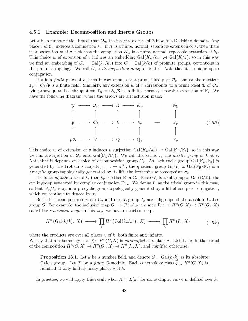
4.5.1 Example: Decomposition and Inertia Groups
Let k be a number field. Recall that Ok, the integral closure of Z in k, is a Dedekind domain. Anyplace v of Ok induces a completion kv. If K is a finite, normal, separable extension of k, then thereis an extension w of v such that the completion Kw is a finite, normal, separable extension of kv.This choice w of extension of v induces an embedding Gal
(Kw/kv
)↪→ Gal
(K/k
), so in this way
we find an embedding of Gv = Gal(kv/kv
)into G = Gal
(k/k
)of profinite groups, continuous in
the profinite topology. We call Gv a decomposition group of k at v. Note that it is unique up toconjugation.
If v is a finite place of k, then it corresponds to a prime ideal p of Ok, and so the quotientFp = Ok/p is a finite field. Similarly, any extension w of v corresponds to a prime ideal P of OKlying above p, and so the quotient FP = OK/P is a finite, normal, separable extension of Fp. Wehave the following diagram, where the arrows are all inclusion maps:
P −−−−→ OK −−−−→ K −−−−→ Kwx x x xp −−−−→ Ok −−−−→ k −−−−→ kvx x x xpZ −−−−→ Z −−−−→ Q −−−−→ Qp
=⇒
FPxFpxFp
(4.5.7)
This choice w of extension of v induces a surjection Gal(Kw/kv
)� Gal
(FP/Fp
), so in this way
we find a surjection of Gv onto Gal(FP/Fp
). We call the kernel Iv the inertia group of k at v.
Note that it depends on choice of decomposition group Gv. As each cyclic group Gal(FP/Fp
)is
generated by the Frobenius map Frp : a 7→ aNp, the quotient group Gv/Iv ' Gal(FP/Fp
)is a
procyclic group topologically generated by its lift, the Frobenius automorphism σv.
If v is an infinite place of k, then kv is either R or C. Hence Gv is a subgroup of Gal(C/R
), the
cyclic group generated by complex conjugation Fr∞. We define Iv as the trivial group in this case,so that Gv/Iv is again a procyclic group topologically generated by a lift of complex conjugation,which we continue to denote by σv.
Both the decomposition group Gv and inertia group Iv are subgroups of the absolute Galoisgroup G. For example, the inclusion map Gv → G induces a map Resv : Hn(G,X)→ Hn(Gv, X)called the restriction map. In this way, we have restriction maps
Hn(Gal(k/k
), X
)−−−−→
∏v
Hn(Gal(kv/kv
), X
)−−−−→
∏v
Hn (Iv, X) (4.5.8)
where the products are over all places v of k, both finite and infinite.
We say that a cohomology class ξ ∈ Hn(G,X) is unramified at a place v of k if it lies in the kernelof the composition Hn(G,X)→ Hn(Gv, X)→ Hn(Iv, X), and ramified otherwise.
Proposition 13.1. Let k be a number field, and denote G = Gal(k/k
)as its absolute
Galois group. Let X be a finite G-module. Each cohomology class ξ ∈ Hn(G,X) isramified at only finitely many places v of k.
In practice, we will apply this result when X ⊆ E[m] for some elliptic curve E defined over k.
48

Proof. We use Proposition 4.1.2. As ξ : G× · · · ×G → X has finite image, there exists a normal,open subgroup U such that the map factors as
ξ : G× · · · ×G −−−−→ (G/U)× · · · × (G/U) −−−−→ X. (4.5.9)
We may express G/U ' Gal(K/k) for some finite, normal, separable extension K of k. But thereare only finitely many places v of k which ramify in K, so the result follows.
49

50

Part I
Selmer Groups
51


4.6 History
4.6.1 Lind and Reichardt’s Quartic
Proposition 4.6.1. Let k be a field of characteristic different from 2 and 17. Consider the quarticcurve C : 2w2 = 1− 17 z4.
1. C is a principal homogeneous space for the elliptic curve E : y2 = x3 + 17x. In particular,E acts continuously and transitively on C via the map � : E × C → C given by
(x, y)� (z, w)
=
(2w y + (x2 − 17) z
(x2 + 17) + 34x z2,w[x4 − 172
]− 34 z
[xw z (x2 − 17) + y (2x+ 17 z2 + x2 z2)
][(x2 + 17) + 34x z2
]2).
(4.6.1)
2. Denoting the elliptic curve E′ : y2 = x3 − 68x, there are rational maps ϕ′ : E → E′ andg : C → E′ defined over k which make the following diagram commute:
E
f
��
ϕ′ // E′
C
g
>> (4.6.2)
Moreover, g(P �Q) = ϕ′(P )⊕ g(Q) for all P on E and Q on C.
3. If C has a k-rational point Q0 = (z0, w0), then C and E are birationally equivalent over k.
Lind and Reichardt studied this quartic equation over k = Q and its completions kv = Qp andR. Then showed that C : 2w2 = 1 − 17 z4 has a Qv-rational point for every place v of Q, yet ithas no Q-rational point. We will see later that we can use properties of the Selmer group to betterunderstand this phenomenon.
Proof. Denote X = E(k) as the collection of k-rational points P = (x, y) on the cubic curveE : y2 = x3 + 17x. As its discriminant is a nonzero ∆ = −26 · 173, we see that E is an ellipticcurve defined over k. Recall that X is a G-module by Proposition 3.1.1. Denote Y = C(k) asthe collection of k-rational points Q = (z, w) the quartic curve C : 2w2 = 1 − 17 z4. The mapf : E → C defined by
f(x, y) =
(√2
y
x2 + 17,
1√2
x2 − 17
x2 + 17
)where f(O) =
(0,
1√2
)(4.6.3)
is a bijection from X to Y which is defined over the finite, normal, separable extension K = k(√
2)of k. Using the identity (x, y)⊕ (0, 0) =
(17/x, −17 y/x2
)for the group law on E, one checks that
for any σ in G = Gal(k/k
)we have the relation
σ[f(P )
]= f
((σ P )⊕ ξ(σ)
)where ξ(σ) =
{(0, 0) if σ(
√2) = −
√2;
O if σ(√
2) = +√
2.(4.6.4)
53
Proposition 3.1.4 states that Y = C(k) is a principal homogeneous space for X = E(k). The map� : X × Y → Y above is defined by (x, y)� (z, w) = f
((x, y)⊕ f−1(z, w)
).
We have seen before that there is a 2-isogeny ϕ′ : E → E′ defined by
ϕ′(x, y) =
(x2 + 17
x, y
x2 − 17
x2
)=⇒
(ϕ′ ◦ f−1
)(z, w) =
(2
z2,
4w
z3
). (4.6.5)
Since im ξ ={
(0, 0), O}
= E[ϕ′], the second statement in the proposition above follows fromProposition 3.1.4.
Finally, say that Q0 = (z0, w0) is a k-rational point on C. Since
x =1− 17 z2 z2
0 + 2ww0
(z − z0)2
y =34 z z0 (z2w0 + z2
0 w)− 2 (w + w0)
(z − z0)3
(4.6.6)
if and only if
z = z0 + 2−w0 y + 17 z3
0 x+ 17 z0
x2 + 34 z20 x+ 17
w = w0 − 34z0
(z2
0 x2 + 2x+ 17 z2
0
)y + w0
(3 z2
0 x3 + 34 z4
0 x2 + x2 + 17z2
0 x+ 17)(
x2 + 34 z20 x+ 17
)2(4.6.7)
we see that the quartic curve 2w2 = 1 − 17 z4 is birationally equivalent over k to the cubic curvey2 = x3 + 17x.
First say that p is a prime such that p - 3D and p ≡ 2 (mod 3). The group homomorphismGm(Fp) → Gm(Fp) defined by z 7→ z3 is injective. Actually, z3 = a if and only if z = aq in termsof q = (2p− 1)/3. Hence we have a bijection
P1(Fp)→ C(Fp) defined by (z1 : z0) 7→(Bq z1 : −
(Az3
1 + C z30
)q: Bq z0
).
In particular, this shows that #C(Fp) = #P1(Fp) = p + 1. Now say that p is a prime such thatp - 3D and p ≡ 1 (mod 3).
Cassel’s Construction
Proposition. Let k be a field of characteristic different from 2 and 3. Consider thequartic curve C : w2 = a4 z
4 + a3 z3 + a2 z
2 + a1 z + a0 as well as the cubic curve
E : y2 = x3+−a2
2 + 3 a1 a3 − 12 a0 a4
3x+
2 a32 − 9 a1 a2 a3 + 27 a0 a
23 + 27 a2
1 a4 − 72 a0 a2 a4
27.
1. C is a principal homogeneous space for the elliptic curve E. In particular, E actscontinuously and transitively on C via the map � : E × C → C given by
(x, y)� (z, w)
= (?, ?) .(4.6.8)
54

2. There are rational maps [2] : E → E and g : C → E defined over k which makethe following diagram commute:
E
f
��
[2] // E
C
g
?? (4.6.9)
Moreover, g(P �Q) = [2]P ⊕ g(Q) for all P on E and Q on C.3. If C has a k-rational point Q0 = (z0, w0) with w0 6= 0, then C and E are bira-
tionally equivalent over k. Moreover, the cubic curve E contains the rational point(x0, y0) = g(z0,−w0).
Proof. Define the map f : E → C by
f(x, y) =
(z0 + w0
2 (x− x0)
(y − y0) + µ (x− x0), w0
(x− x0)3 + 2 y0
((y − y0) + µ (x− x0)
)+ 2 ν (x− x0)(
(y − y0) + µ (x− x0))2
)
f(O) =(z0, w0
)in terms of the constants
x0 =
(3 a23 − 8 a2 a4) z4
0 + (4 a2 a3 − 24 a1 a4) z30
+ (4 a22 − 6 a1 a3 − 48 a0 a4) z2
0 + (4 a1 a2 − 24 a0 a3) z0 + (3 a21 − 8 a0 a2)
12w20
y0 =
(−a33 + 4 a2 a3 a4 − 8 a1 a
24) z6
0 + (−2 a2 a23 + 8 a2
2 a4 − 4 a1 a3 a4 − 32 a0 a24) z5
0
+ (−5 a1 a23 + 20 a1 a2 a4 − 40 a0 a3 a4) z4
0
+ (−20 a0 a23 + 20 a2
1 a4) z30 + (5 a2
1 a3 − 20 a0 a2 a3 + 40 a0 a1 a4) z20
+ (2 a21 a2 − 8 a0 a
22 + 4 a0 a1 a3 + 32 a2
0 a4)x0 + (a31 − 4 a0 a1 a2 + 8 a2
0 a3)
8w30
µ = −4 a4 z30 + 3 a3 z
20 + 2 a2 z0 + a1
2w0
ν = −
(8 a33 a4 − 32 a2 a3 a
24 + 64 a1 a
34) z9
0 + (9 a43 − 24 a2 a
23 a4 − 48 a2
2 a24 + 96 a1 a3 a
24 + 192 a0 a
34) z8
0
+ (24 a2 a33 − 96 a2
2 a3 a4 + 48 a1 a23 a4 + 384 a0 a3 a
24) z7
0
+ (16 a22 a
23 + 36 a1 a
33 − 64 a3
2 a4 − 112 a1 a2 a3 a4 + 240 a0 a23 a4 + 48 a2
1 a24 + 256 a0 a2 a
24) z6
0
+ (48 a1 a2 a23 + 72 a0 a
33 − 192 a1 a
22 a4 − 24 a2
1 a3 a4 + 192 a0 a2 a3 a4 + 384 a0 a1 a24) z5
0
+ (30 a21 a
23 + 120 a0 a2 a
23 − 216 a2
1 a2 a4 − 96 a0 a22 a4 + 288 a0 a1 a3 a4 + 384 a2
0 a24) z4
0
+ (−8 a21 a2 a3 + 32 a0 a
22 a3 + 144 a0 a1 a
23 − 96 a3
1 a4 − 256 a0 a1 a2 a4 + 384 a20 a3 a4) z3
0
+ (−12 a31 a3 + 48 a0 a1 a2 a3 + 144 a2
0 a23 − 240 a0 a
21 a4) z2
0
+ (−24 a0 a21 a3 + 96 a2
0 a2 a3 − 192 a20 a1 a4) z0 + (a4
1 − 8 a0 a21 a2 + 16 a2
0 a22 − 64 a3
0 a4)
32w40
55

Notice that E is the Jacobian of C. We have a 2-covering g : C → E defined as follows:
x =1
12
(3 a23 − 8 a2 a4) z4 + 4 (a2 a3 − 6 a1 a4) z3
+ 2 (2 a22 − 3 a1 a3 − 24 a0 a4) z2 + 4 (a1 a2 − 6 a0 a3) z + (3 a2
1 − 8 a0 a2)
a4 z4 + a3 z3 + a2 z2 + a1 z + a0
y =w
8
(a33 − 4 a2 a3 a4 + 8 a1 a
24) z6 − 2 (−a2 a
23 + 4 a2
2 a4 − 2 a1 a3 a4 − 16 a0 a24) z5
+ 5 (a1 a23 − 4 a1 a2 a4 + 8 a0 a3 a4) z4 + 20 (a0 a
23 − a2
1 a4) z3 − 5 (a21 a3 − 4 a0 a2 a3 + 8 a0 a1 a4) z2
− 2 (a21 a2 − 4 a0 a
22 + 2 a0 a1 a3 + 16 a2
0 a4) z − (a31 − 4 a0 a1 a2 + 8 a2
0 a3)(a4 z4 + a3 z3 + a2 z2 + a1 z + a0
)2
Lisker’s Question
Consider the equation
C :x
y+y
z+z
x= n. (4.6.10)
a3 + b3 + c3
abc= n (4.6.11)
looked similar to an elliptic curve, so I thought to translate this conjecture into one explicitlyinvolving an elliptic curve. Fix an integral solution (x, y, z) and make the substitution
u = 3n2z − 12x
z
v = 1082x y − nx z + z2
z2
(4.6.12)
Then (u, v) is a rational point on the elliptic curve
En : v2 = u3 +Au+B whereA = 27n (24− n3)
B = 54 (216− 36n3 + n6)(4.6.13)
4.7 Selmer and Shafarevich-Tate Groups
4.7.1 Classical Definitions
Assume now that k is a number field. Define the f -Selmer, Shafarevich-Tate, and f -Cassels groups,respectively, as
Sel(f)(X/k) = ker
[H1(Gal(k/k
), X[f ]
)−→
∏v
H1(Gal(kv/kv
), X
)]
III(X/k) = ker
[H1(Gal(k/k
), X
)−→
∏v
H1(Gal(kv/kv
), X
)]
Cas(f)(X/k) = ker
[H2(Gal(k/k
), X[f ]
)−→
∏v
H2(Gal(kv/kv
), X[f ]
)](4.7.1)
56

Note that the Selmer and Shafarevich-Tate groups are subgroups of the Weil-Chatalet group ofX[f ]. Since f is an isogeny, we see that the elements of these groups are ramified at only finitelymany places v of k.
Then we have the first few cohomology groups
XG = H0(G,X)
ZG = H0(G,Z)
WC(X/k) = H1(G,X)
(4.7.2)
The First Isomorphism Theorem asserts that we have a short exact sequence of G-modules
{O} −−−−→ X[ϕ] −−−−→ Xϕ−−−−→ Z −−−−→ {O} (4.7.3)
The long exact sequence from cohomology asserts that we have the commutative, exact diagram
{O} {O} {O}y y y{O} −−−−→ ZG
ϕ(XG)
δ0−−−−→ Sel(ϕ)(X/k) −−−−→ III(X/k)ϕ∗−−−−→ · · ·y y y
{O} −−−−→ ZG
ϕ(XG)
δ0−−−−→ H1(G,X[ϕ]) −−−−→ H1(G,X)ϕ∗−−−−→ · · ·y y y
{O} −−−−→∏v
H1(Gv, X)'−−−−→
∏v
H1(G,X)
(4.7.4)
4.7.2 Elliptic Curves
Let φ : E′ → E and φ′ : E → E′ be dual m-isogenies of elliptic curves, all of which are defined overa number field k. Define the φ′-Selmer, Shafarevich-Tate, and φ′-Cassels groups, respectively, as
Sel(φ′)(E/k) = ker
[H1(Gal(k/k
), E[φ′]
)−→
∏v
H1(Gal(kv/kv
), E(kv)
)]
III(E/k) = ker
[H1(Gal(k/k
), E(k)
)−→
∏v
H1(Gal(kv/kv
), E(kv)
)]
Cas(φ′)(E/k) = ker
[H2(Gal(k/k
), E[φ′]
)−→
∏v
H2(Gal(kv/kv
), E[φ′]
)](4.7.5)
where the product is over all all places v of k. Note that III(E/k) ⊆ WC(E/k). While the Weil-Chatalet group WC(E/k) = H1
(Gal(k/k
), E(k)
)is known to be infinite, the Shafarevich-Tate
group is conjectured to be finite! The following result shows how these are all related.
Proposition 14.1. Let φ : E′ → E and φ′ : E → E′ be dual m-isogenies of ellipticcurves, all of which are defined over a number field k.
57

• We have the short exact sequence
{O} −−−−→ E′(k)
φ′(E(k)
) δ0−−−−→ Sel(φ′)(E/k) −−−−→ III(E/k)[φ′∗]
φ′∗−−−−→ {O}.
(4.7.6)In particular, the index
[E′(k) : φ′
(E(k)
)]is finite.
• The connecting homomorphism induces an embedding
Sel(φ)(E′/k)
φ′∗ Sel(m)(E/k)
∼−−−−→ III(E′/k)[φ∗]
φ′∗ III(E/k)[m∗]
δ1−−−−→ Cas(φ′)(E/k). (4.7.7)
• With δ1 as above, we have the orders
∣∣∣∣ E′(k)[φ]
φ′(E(k)[m]
)∣∣∣∣ ∣∣∣∣ E(k)
mE(k)
∣∣∣∣ =
∣∣Sel(φ′)(E/k)
∣∣ ∣∣Sel(φ)(E′/k)∣∣∣∣im δ1
∣∣ ∣∣III(E/k)[m∗]∣∣ . (4.7.8)
Tate showed that Cas(m)(E/k) = {1} for a a number field k containing the mth roots of unityfor a prime m = p. Hence, im δ1 = {O} and Sel(φ)(E′/k) = φ′∗ Sel(m)(E/k) in this case.
Proof. We have the following collection of short exact sequences:
{O} −−−−→ E[φ′] −−−−→ E[m]φ′−−−−→ E′[φ] −−−−→ {O}y y y
{O} −−−−→ E[φ′] −−−−→ E(k)φ′−−−−→ E′(k) −−−−→ {O}
(4.7.9)
The Long Exact Sequence for Cohomology (Theorem 4.4.1) induces the following commutativediagram with exact rows and exact columns:
{O} −−−−→ E′(k)
φ′(E(k)
) δ0−−−−→ H1(G, E[φ′]
)−−−−→ H1
(G, E(k)
)[φ′∗]
φ′∗−−−−→ {O}yφ y y{O} −−−−→ E(k)
mE(k)
δ0−−−−→ H1(G, E[m]
)−−−−→ H1
(G, E(k)
)[m∗]
m∗−−−−→ {O}y yφ′∗ yφ′∗{O} −−−−→ E(k)
φ(E′(k)
) δ0−−−−→ H1(G, E′[φ]
)−−−−→ H1
(G, E′(k)
)[φ∗]
φ∗−−−−→ {O}
(4.7.10)
Upon choosing embeddings of k into completions kv, we have embeddings of Gv = Gal(kv/kv
)into
58
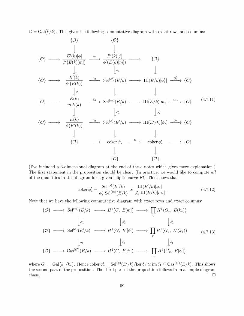
G = Gal(k/k
). This gives the following commutative diagram with exact rows and columns:
{O} {O}y y{O} −−−−→ E′(k)[φ]
φ′(E(k)[m]
) '−−−−→ E′(k)[φ]
φ′(E(k)[m]
) −−−−→ {O}y yδ0 y{O} −−−−→ E′(k)
φ′(E(k)
) δ0−−−−→ Sel(φ′)(E/k) −−−−→ III(E/k)[φ′∗]
φ′∗−−−−→ {O}yφ y y{O} −−−−→ E(k)
mE(k)
δ0−−−−→ Sel(m)(E/k) −−−−→ III(E/k)[m∗]m∗−−−−→ {O}y yφ′∗ yφ′∗
{O} −−−−→ E(k)
φ(E′(k)
) δ0−−−−→ Sel(φ)(E′/k) −−−−→ III(E′/k)[φ∗]φ∗−−−−→ {O}y y y
{O} −−−−→ cokerφ′∗'−−−−→ cokerφ′∗ −−−−→ {O}y y
{O} {O}
(4.7.11)
(I’ve included a 3-dimensional diagram at the end of these notes which gives more explanation.)The first statement in the proposition should be clear. (In practice, we would like to compute allof the quantities in this diagram for a given elliptic curve E!) This shows that
cokerφ′∗ =Sel(φ)(E′/k)
φ′∗ Sel(m)(E/k)' III(E′/k)[φ∗]
φ′∗ III(E/k)[m∗]. (4.7.12)
Note that we have the following commutative diagram with exact rows and exact columns:
{O} −−−−→ Sel(m)(E/k) −−−−→ H1(G, E[m]
)−−−−→
∏v
H1(Gv, E(kv)
)yφ′∗ yφ′∗ yφ′∗
{O} −−−−→ Sel(φ)(E′/k) −−−−→ H1(G, E′[φ]
)−−−−→
∏v
H1(Gv, E
′(kv))
yδ1 yδ1 yδ1{O} −−−−→ Cas(φ′)(E/k) −−−−→ H2
(G, E[φ′]
)−−−−→
∏v
H2(Gv, E[φ′]
)(4.7.13)
where Gv = Gal(kv/kv
). Hence cokerφ′∗ = Sel(φ)(E′/k)/ker δ1 ' im δ1 ⊆ Cas(φ′)(E/k). This shows
the second part of the proposition. The third part of the proposition follows from a simple diagramchase.
59
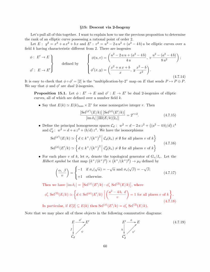
§15: Descent via 2-Isogeny
Let’s pull all of this together. I want to explain how to use the previous proposition to determinethe rank of an elliptic curve possessing a rational point of order 2.
Let E : y2 = x3 + a x2 + b x and E′ : v2 = u3 − 2 a u2 + (a2 − 4 b)u be elliptic curves over afield k having characteristic different from 2. There are isogenies
φ : E′ → E
φ′ : E → E′
defined by
φ(u, v) =
(u2 − 2 a u+ (a2 − 4 b)
4u, v
u2 − (a2 − 4 b)
8u2
);
φ′(x, y) =
(x2 + a x+ b
x, y
x2 − bx2
).
(4.7.14)It is easy to check that φ ◦ φ′ = [2] is the “multiplication-by-2” map on E that sends P 7→ P ⊕ P .We say that φ and φ′ are dual 2-isogenies.
Proposition 15.1. Let φ : E′ → E and φ′ : E → E′ be dual 2-isogenies of ellipticcurves, all of which are defined over a number field k.
• Say that E(k) ' E(k)tors × Zr for some nonnegative integer r. Then∣∣Sel(φ′)(E/k)
∣∣ ∣∣Sel(φ)(E′/k)∣∣∣∣im δ1
∣∣ ∣∣III(E/k)[2∗]∣∣ = 2r+2. (4.7.15)
• Define the principal homogeneous spaces Cd : w2 = d − 2 a z2 +((a2 − 4 b)/d
)z4
and C′d : w2 = d+ a z2 + (b/d) z4. We have the isomorphisms
Sel(φ′)(E/k) '
{d ∈ k×/
(k×)2 ∣∣∣ Cd(kv) 6= ∅ for all places v of k
}Sel(φ)(E′/k) '
{d ∈ k×/
(k×)2 ∣∣∣ C′d(kv) 6= ∅ for all places v of k
} (4.7.16)
• For each place v of k, let σv denote the topological generator of Gv/Iv. Let theHilbert symbol be that map
(k×/(k×)2
)×(k×/(k×)2
)→ µ2 defined by(
α, β
v
)=
−1 if σv(√α) = −
√α and σv(
√β) = −
√β;
+1 otherwise.(4.7.17)
Then we have∣∣im δ1
∣∣ =[Sel(φ)(E′/k) : φ′∗ Sel(2)(E/k)
], where
φ′∗ Sel(2)(E/k) '{d ∈ Sel(φ)(E′/k)
∣∣∣∣ (a2 − 4 b, d
v
)= 1 for all places v of k
}.
(4.7.18)In particular, if E[2] ⊆ E(k) then Sel(φ)(E′/k) = φ′∗ Sel(2)(E/k).
Note that we may place all of these objects in the following commutative diagrams:
Eφ′ //
f
��
E′
Cdψ
?? E′φ //
h��
E
C′dψ′
?? (4.7.19)
60

in terms of the maps
f(x, y) =
( √d y
x2 + a x+ b,
√d (x2 − b)
x2 + a x+ b
)ψ(z, w) =
(d
z2,dw
z3
)
h(u, v) =
( √d v
u2 − 2 a u+ (a2 − 4 b),
√d(u2 − (a2 − 4 b)
)u2 − 2 a u+ (a2 − 4 b)
)ψ′(z, w) =
(d
z2,dw
z3
)(4.7.20)
(You may wish to compare with the maps in §4.) This gives an explicit way to compute the Mordell-Weil rank r, assuming of course that the subgroup of the Shafarevich-Tate group III(E/k)[2∗] istrivial. The idea is to find kv-rational points on principal homogeneous spaces.
Proof. We can write E(k)tors ' E(k)[2∞]×T , where T is a finite group of odd order. Upon writing∣∣E(k)tors ∩ E[2]∣∣ = 2e, we have the expressions
E′(k)[φ]
φ′(E(k)[2]
) ' Z22−e and
E(k)
2E(k)' Z2
r+e =⇒∣∣∣∣ E′(k)[φ]
φ′(E(k)[2]
)∣∣∣∣ ∣∣∣∣ E(k)
2E(k)
∣∣∣∣ = 2r+2. (4.7.21)
The first statement in the proposition follows from Proposition 14.1.We prove the latter two statements. Consider the short exact sequence
{O} −−−−→ E[φ′] −−−−→ E[2]φ′−−−−→ E′[φ] −−−−→ {O}. (4.7.22)
The Long Exact Sequence for Cohomology (Theorem 4.4.1) induces the following exact sequence:
H1(G, E[2]
) φ′∗−−−−→ H1(G, E′[φ]
) δ1−−−−→ H2(G, E[φ′]
). (4.7.23)
We follow the proof of Theorem 4.4.1 to compute δ1. Choose ξ ∈ H1(G, E′[φ]
). For any σ ∈ G
we have ξ(σ) ∈ E′[φ] ={O, (0, 0)
}, so that [2] ξ(σ) = O. Using Proposition 13.1 (or better yet,
following the proof of Proposition 4.1.2), we see that there exists d ∈ k× such that
ξ(σ) =
(0, 0) if σ(√d) = −
√d;
O if σ(√d) = +
√d.
(4.7.24)
Hence the map k×/(k×)2 → H1
(G, E′[φ]
)defined by d 7→ ξ is actually an isomorphism. In fact,
the discussion in §5 and Theorem 4.2.1 prove the second statement in the proposition. As the mapφ′ : E[2]→ E′[φ] is surjective, we have ξ = φ′∗ β for β ∈ C1
(G, E[2]
), where
β(σ) =
((−a+
√a2 − 4 b)/2, 0
)if σ(√a2 − 4 b) = −
√a2 − 4 b and σ(
√d) = −
√d;(
(−a−√a2 − 4 b)/2, 0
)if σ(√a2 − 4 b) = +
√a2 − 4 b and σ(
√d) = −
√d;(
0, 0)
if σ(√a2 − 4 b) = −
√a2 − 4 b and σ(
√d) = +
√d;
O if σ(√a2 − 4 b) = +
√a2 − 4 b and σ(
√d) = +
√d.
(4.7.25)
It is easy to verify that
β(σ) =(∂0 P
)(σ) = where P =
?? if σ(√d) = −
√d;(
(−a+√a2 − 4 b)/2, 0
)if σ(√d) = +
√d.
(4.7.26)
61

Consider the quadric intersection Hd1,d2 : x>Ax = x>Bx = 0 in P3 defined in terms of
A =
d1 0 0 00 −d2 0 00 0 0 0
0 0 0(a−√a2 − 4 b
)/2
and B =
d1 0 0 00 0 0 00 0 −d1 d2 0
0 0 0(a+√a2 − 4 b
)/2
.(4.7.27)
We have the following diagram:
E∼ //
f
��
Eφ′ //
g
��
E′
Cd
ψ
??
// H1,d
?? Eφ′ //
g
��
E′φ //
h
��
E
Hd1,d2
??
φ′∗
// C′d1
ψ
?? (4.7.28)
in terms of the maps
g(x, y) =
(x2 − b2√d1 y
:x2 +
(a−√a2 − 4 b
)x+ b
2√d2 y
:x2 +
(a+√a2 − 4 b
)x+ b
2√d1 d2 y
: 1
)
φ′∗ (x1 : x2 : x3 : x0) =
(x0
x1,d2 x2 x3
x21
)
(z, w) 7→
(w
2 z:d−√a2 − 4 b z2
2 d z:d+√a2 − 4 b z2
2 d z: 1
)(4.7.29)
(Recall that this is not the only choice of β!) We compute α = ∂1 β ∈ C2(G, E[2]
)as
α(σ, τ) =(σ β(τ)
)⊕(−β(σ ◦ τ)
)⊕ β(σ)
=
(0, 0) if σ(√a2 − 4 b) = −
√a2 − 4 b and τ(
√d) = −
√d;
O otherwise.
(4.7.30)
Since α ∈ Z2(G, E[φ′]
), we define δ1 ξ = α ∈ H2
(G, E[φ′]
). Recall the following diagram:
{O} −−−−→ Sel(2)(E/k) −−−−→ H1(G, E[2]
)−−−−→
∏v
H1(Gv, E(kv)
)yφ′∗ yφ′∗ yφ′∗
{O} −−−−→ Sel(φ)(E′/k) −−−−→ H1(G, E′[φ]
)−−−−→
∏v
H1(Gv, E
′(kv))
yδ1 yδ1 yδ1{O} −−−−→ Cas(φ′)(E/k) −−−−→ H2
(G, E[φ′]
)−−−−→
∏v
H2(Gv, E[φ′]
)(4.7.31)
62

We must verify that if ξ ∈ Sel(φ)(E′/k) we have α ∈ Cas(φ′)(E/k). Actually, it suffices for ourpurposes to determine when α = O. Note that(
ker δ1
)∩ Sel(φ)(E′/k) =
(imφ′∗
)∩ Sel(φ)(E′/k)
= φ′∗ Sel(2)(E/k)
=
{ξ = φ′∗ β
∣∣∣∣∣ β ∈ Z1(G, E[2]
)and
Resv β ∈ B1(Gv, E(kv)
)for all places v of k
}.
(4.7.32)
Consider the composition
k×(k×)2 ∼−−−−→ H1
(G, E′[φ]
) δ1−−−−→ H2(G, E[φ′]
)−−−−→
∏v
H2(Gv, E[φ′]
). (4.7.33)
This composition is uniquely determined by the image α(σv, σv). We see that
φ′∗ Sel(2)(E/k) = ker[Sel(φ)(E′/k) −→ Cas(φ′)(E/k)
]'{d ∈ Sel(φ)(E′/k)
∣∣∣∣ (a2 − 4 b, d
v
)= +1 for all places v of k
}.
(4.7.34)
If E[2] ⊆ E(k), then√a2 − 4 b ∈ k×, so that δ1 : ξ 7→ O is the trivial map.
§16: Example: Notes to Cremona
Let me work out a more specific example. You’ll recall the elliptic curves we sent to Cremona:
E : y2 + x y = x3 − 1568667218344734400688655080x
+ 23913566028813160045118782083988547150400
E′ : v2 + u v = u3 − 1569352275530075968688655080u
+ 23891634009988359905502318672762947150400
(4.7.35)
(E and E′ are switched from what I have listed here to what I have in the notes to Cremona.) Itis easy to verify that
a = 274413197622721
b = 2192182993093017600000000
}=⇒ a2−4 b = 2521 ·5641 ·
(72763777009
)2. (4.7.36)
We found using mwrank that
E(Q) ' Z8 × Z2 E′(Q) ' Z2 × Z8 × Z2
Sel(φ′)(E/Q) ' Z2
4 '⟨100578403849, 4081, 4369, 2521
⟩Sel(φ)(E′/Q) ' Z2
2 '⟨−13, 15
⟩Sel(2)(E/Q) ' Z2
3 Sel(2)(E′/Q) ' Z26
III(E/Q) ' {1} III(E′/Q) ' Z22
(4.7.37)
63

Since E′[2] ⊆ E′(Q), it is clear that φ∗ Sel(2)(E′/k) = Sel(φ′)(E/k); fortunately, mwrank verifies this.
We wish to compute φ′∗ Sel(2)(E/k) ⊆ Sel(φ)(E′/k); you’ll recall that mwrank does not compute thiscorrectly. By considering the set of “bad” primes for these elliptic curves, in order to compute theimage of the connecting homomorphism, we must compute the value of the Hilbert symbol(
2521 · 5641, d
v
)for
{d ∈ {−195, −13, 1, 15};v ∈ {2, 3, 5, 7, 11, 13, 17, 53, 257, 2521, 5641, ∞}.
(4.7.38)
Hence im δ1 = 〈−13, 15〉 = Sel(φ)(E′/k), so that φ′∗ Sel(2)(E/k) ' {1}.
64
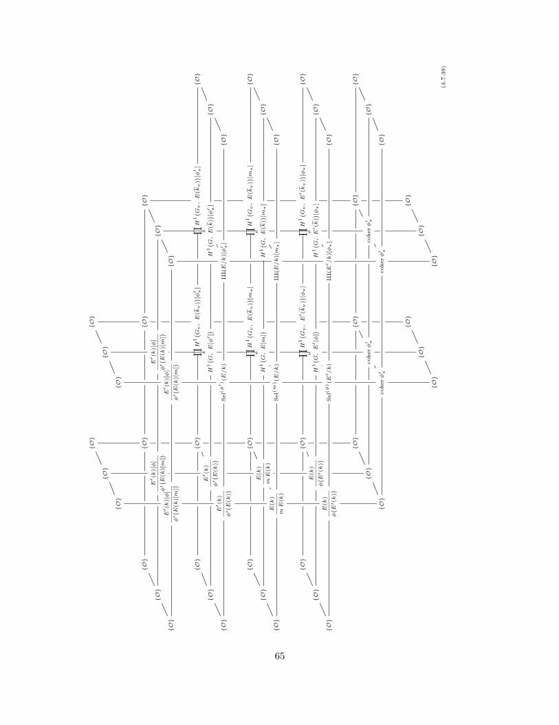
{O}
{O}
{O}
{O}
{O}
{O}
{O}
{O}
{O}
{O}
{O}
E′ (k)[φ]
φ′( E
(k)[m
])E′ (k)[φ]
φ′( E
(k)[m
]){O}
{O}
E′ (k)[φ]
φ′( E
(k)[m
])E′ (k)[φ]
φ′( E
(k)[m
]){O}
{O}
{O}
∏ v
H1( G v
,E(kv)) [φ′ ∗]
∏ v
H1( G v
,E(kv)) [φ′ ∗]
{O}
{O}
E′ (k)
φ′( E
(k))
H1( G,
E[φ′ ])
H1( G,
E( k
)) [φ′ ∗]
{O}
{O}
E′ (k)
φ′( E
(k))
Sel(φ′ )(E/k)
III(E/k)[φ′ ∗]
{O}
{O}
{O}
∏ v
H1( G v
,E(kv)) [m
∗]
∏ v
H1( G v
,E(kv)) [m
∗]
{O}
{O}
E(k
)
mE(k
)H
1( G,
E[m
])H
1( G,
E( k
)) [m∗]
{O}
{O}
E(k
)
mE(k
)Sel(m
)(E/k)
III(E/k)[m∗]
{O}
{O}
{O}
∏ v
H1( G v
,E′ (kv)) [φ∗]
∏ v
H1( G v
,E′ (kv)) [φ∗]
{O}
{O}
E(k
)
φ( E′
(k))
H1( G,
E′ [φ])
H1( G,
E′ (k)) [φ∗]
{O}
{O}
E(k
)
φ( E′
(k))
Sel(φ)(E′ /k)
III(E′ /k)[φ∗]
{O}
{O}
{O}
{O}
{O}
{O}
cokerφ′ ∗
cokerφ′ ∗
{O}
{O}
cokerφ′ ∗
cokerφ′ ∗
{O}
{O}
{O}
{O}
{O}
{O}
{O}
(4.7.39)
65