Self%tuning+Transac1onal+Memory+ via+Machine+Learning++

Self-‐tuning Transac1onal Memory via Machine Learning

and Analy1cal Modeling

Paolo Romano

INESC-‐ID Ins+tuto Superior Técnico, Lisbon University

Roadmap • Background on Transactional Memory

•  alternative implementations

•  TM performance tuning

• Gray box based self-tuning •  Provisioning and optimization of a Distributed TM •  Divide and conquer •  Bootstrapping •  Hybrid ensembling

Multi-cores are now ubiquitous

The multi-core (r)evolution Shared Memory

CPU1

CPU2

CPU3

CPU4

Concurrent programming is complex

Hard to get right: •  fine-grained locks •  deadlocks •  correctness

Classic approach: Locking

atomic { withdraw(acc1,val); deposit(acc2,val); }

Transactional Memory abstraction

Programmer identifies atomic blocks Runtime implements synchronization

Transactional Memory System

(A very incomplete) Historical perspective on TM

Hardware TM

[ISCA]

1993 1995

Software TM

[PODC]

2005

1st Intel dual core

CPU

2014

1st Intel CPU with

HTM

Intel’s Haswell CPU targets mainstream computing platforms: •  including desktops, servers, laptops, and tablets Recently also IBM has integrated HTM supports in its high-end CPUs: •  BG/Q, zEC12, Power8

Transactional Memory: One abstraction, many implementations

•  Software (STM): •  instrumenting read and write accesses

•  PRO: flexibility •  CON: instrumentation overheads

•  Hardware (HTM): •  extension of the cache consistency mechanism

•  PRO: no instrumentation overheads •  CON: hw is inherently limited

•  Hybrid (HyTM) •  mix of the two worlds that tries to achieve the best of both

•  Distributed (DTM)

•  natural extension of TM for distributed shared memory •  PRO: fault-tolerance, potential for higher scalability •  CON: synchronization costs are amplified

Automatic Tuning of the Parallelism Degree in Hardware Transactional Memory – EuroPar 2014 6

Software TM

int i = 0

…

atomic { i++}

int i = 0…TM.begin-tx()int tmp = TM.read(&i)tmp++TM.write(&i, tmp)TM.end-tx()

Source program Compiled program

instrumentation to invoke STM

•  Non-negligible instrumentation overheads

•  Highly flexible: •  Avoid inherent restrictions of hardware implementations

•  Over 10 years of research on STM è highly optimized prototypes and designs









HTM: Intel Transactional Synchronization Extensions (TSX)

CPU1

CPU2

Memory Bus

L1 Cache

L1 Cache

L2 Cache L2 Cache

L3 Cache

CPU 1 CPU 2

xbegin

TSX: on

read x: 0 // Set bit read on x cache line

x: 0 -- r

write y = 1 // Buffer write in L1 cache

y: 1 -- w

xend // Atomically clean bits and publish

x: 0 y: 1

xbegin read y: 1

write y = 2

xabort

invalidation snooped write invalidates tx read

…

…

y: 1 -- r x: 0 y: 2

Restrictions of TSX No progress guarantees:

•  A transaction may always abort

…due to a number of reasons:

•  Forbidden instructions

•  Capacity of caches

•  Faults and signals

•  Contending transactions, aborting each other









Distributed Transactional Memory 11 Automatic Tuning of the Parallelism Degree in Hardware Transactional Memory – EuroPar 2014

• Extends the reach of TM abstraction to distributed applications

• Enhanced scalability, high-availability and fault-tolerance

• Attractive paradigm for the cloud

At the convergence of two areas 12 Automatic Tuning of the Parallelism Degree in Hardware Transactional Memory – EuroPar 2014

Transac1ons allow to:

1.  Deal with remote data races 2.  Boost performance by batching remote

synchroniza+ons during commit phase

•  Natural source of inspira+on for DSTMs... •  but DSTMs have unique requirements,

e.g.: •  >70% txs are 100x shorter in DSTM

Distributed Shared Memory Distributed Databases

Distributed Transactional Memory





TM performance tuning •  TM abstraction allows for encapsulating a vast range of

alternative implementation strategies •  no one size fits all solution [SPAA08, PACT14]

• Each implementation comes with various tuning-knobs: •  number of retries in HTM [ICAC14] •  granularity of locks in STM [PPoPP08]

• Parallelism degree: •  how many threads should be concurrently active? [EuroPar14]

•  Thread mapping: •  on which cores should the active threads be executed? [JPDC14]

14 Automatic Tuning of the Parallelism Degree in Hardware Transactional Memory – EuroPar 2014

TM tuning: no one size fits all 15 Automatic Tuning of the Parallelism Degree in Hardware Transactional Memory – EuroPar 2014

ASPLOS Submission #137– Confidential Draft – Do Not Distribute!!

ProteusTM: Abstraction Meets Performance in Transactional Memory

AbstractThe Transactional Memory (TM) paradigm promises to

greatly simplify the development of concurrent applications.This led, over the years, to the creation of a plethora of TMimplementations delivering wide ranges of performance acrossworkloads. Yet, no universal TM implementation fits each andevery workload. In fact, the best TM in a given workload canreveal to be disastrous for another one. This forces developersto face the complex task of tuning TM implementations, whichsignificantly hampers the wide adoption of TMs.

In this paper, we address the challenge of automaticallyidentifying the best TM implementation for a given workload.Our proposed system, ProteusTM, hides behind the TM inter-face a large library of implementations. Under the hood, itleverages an innovative, multi-dimensional online optimiza-tion scheme, combining two popular machine learning tech-niques: Collaborative Filtering and Bayesian Optimization.

We integrated ProteusTM in GCC and demonstrated itsability to switch TM implementations and adapt several con-figuration parameters (e.g., number of threads). We extensivelyevaluated ProteusTM, obtaining average performance < 3%from optimal, and gains up to 100⇥ over static alternatives.

1. IntroductionThe advent of multi-cores has brought parallel computing tothe fore-front of software development, fostering research onparadigms to simplify the development of concurrent applica-tions. The Transactional Memory (TM) [35] abstraction is aprominent approach that promotes a simple idiom for synchro-nizing code: programmers specify only what should be doneatomically (via serializable transactions), leaving to the TMthe responsibility of implementing how to achieve it.

Over time, several works have provided evidence [57, 46,52] on the effectiveness of TM to simplify the developmentand verification of concurrent programs, enhancing code reli-ability and productivity. Recently, the relevance of TM wasamplified by the standardization of constructs in popular lan-guages (such as C/C++ [49]), and by the integration of hard-ware support in processors by Intel and IBM [67, 39].The abstraction vs performance dilemma. Unfortunately,TM performance remains a controversial matter [11]: despitethe large body of work in the area, the search for a “univer-sal” TM with optimal performance across all workloads hasbeen unsuccessful.Fig. 1 conveys experimental evidence ofthe strong sensitivity of TM to the workload characteristics.We report on the energy efficiency (in Fig. 1a) and through-put (in Fig. 1b) of various TMs in different architectures andbenchmarks. We normalized the data with respect to the best

0

0.2

0.4

0.6

0.8

1

genome red-black tree labyrinth

Nor

mal

ized

wrt

best NOrec:4t

Tiny:8tHTM:8t

(a) Throughput/Joule on a single-chip8-core CPU (Machine A in Table 2).

0

0.2

0.4

0.6

0.8

1

vacation red-black tree intruder

Nor

mal

ized

wrt

best NOrec:48t

Tiny:8t

Swiss:32t

(b) Throughput on a multi-chip 32-core CPU (Machine B in Table 2).

Figure 1: Performance heterogeneity in TM applications.

performing configuration for the considered workload. Fig. 1shows that, in two different architectures and metrics, theoptimal TM configuration differs significantly for each work-load. Furthermore, choosing wrong configurations can crippleperformance by several orders of magnitude. Interestingly,some TMs used in these experiments were designed to tacklevarious workloads [29, 27], but configuring them properly isnon-trivial and they still cannot perform well for all workloads.

The problem is that the efficiency of existing TM imple-mentations is strongly dependent on the workloads they face.Performance can be affected by a number of factors, includingprogram inputs [26], phases of program execution [24], tuningof the internal parameters of the TM algorithms [25], as wellas architectural aspects of the underlying hardware [12].

Given the vast TM design space, manually identifying opti-mal configurations, using trial and error on each workload, is adaunting task. Overall, the complexity associated with tuningTM contradicts the motivation at its basis, i.e., to simplifythe life of programmers, and represents a roadblock to theadoption of TM as a mainstream paradigm [42].Contributions. We propose a new system, ProteusTM1,which allows developers to still enjoy the simplicity and easeof usage of the TM abstraction, while sparing them from theburden of tuning TM implementations to specific workloads.

Under the simple and elegant interface of TM, ProteusTMhides a large library of TM implementations. At run-time,ProteusTM relies on an innovative combination of learningtechniques to pursue optimal efficiency via multi-dimensionaladaptation of the TM implementation and its parameters.

At the heart of ProteusTM lie two key components:• PolyTM is a polymorphic TM library that encapsulates state-of-the-art results from research in TM, and has the uniqueability to transparently and dynamically adapt across multipledimensions: (i) switch between different TM algorithms; (ii)reconfigure the internal parameters of a TM; (iii) adapt thenumber of threads concurrently generating transactions.• RecTM is in charge of determining the optimal TM config-

1Proteus is a Greek god who can foretell the future and adapt his shape.

Benchmark Lines of Code Atomic Blocks DescriptionSTAMP [9] 28803 35 Suite of 8 heterogeneous benchmarks with a variety of workloads (genomics, graphs, databases).Data Structures 3702 12 Concurrent Red-Black Tree, Skip-List, Linked-List and Hash-Map with workloads varying contention and update ratio.STMBench7 [32] 8623 45 Based on OO7 [10] with many heterogeneous transactions over a large and complex graph of objects.TPC-C [63] 6690 5 OLTP workload with in-memory storage adapted to use one atomic block encompassing each transaction.Memcached [58] 12693 120 Caching service with many short transactions that are used to read and update the cache coherently.

Table 1: TM applications used in our evaluation. These 15 benchmarks span a wide variety of workloads and characteristics.

Machine ID Processor / Number of cores / RAM HTM RAPLMachine A 1 Intel Haswell Xeon E3-1275 3.5GHz /

4 (8 hyper-threads) / 32 GBYes Yes

Machine B 4 AMD Opteron 6172 2.1 Ghz / 48 / 32 GB No No

Table 2: Machines used in our experimental test-bed.

More in detail, the Controller builds a bagging ensemble [7]of k CF learners, each trained on a random subset of thetraining set. Then, it computes µx as the average of the valuesoutput by the single predictors, and s2

x as their variance. InProteusTM, we use 10 bagged models; we highlight that thecost of employing them instead of a single one is negligible,mainly because they are only queried during profiling phases.Stopping Criterion. As discussed, SMBO requires the defi-nition of a predicate to stop exploring new configurations.

Our Controller uses a stopping criterion that seeks a bal-ance between exploration and exploitation by relying on thenotion of EI: it uses the estimated likelihood that additionalexplorations may lead to better configurations. More precisely,the exploration is terminated after k steps when: (i) the EIdecreased in the last 2 iterations; (ii) the EI for the k-th ex-ploration was marginal, i.e., lower than e with respect to thecurrent best sampled KPI; (iii) the relative performance im-provement achieved in the k�1-th iteration did not exceed e .In §6.3, we evaluate the effectiveness of this policy.

5.3. Monitor: Lightweight Behavior Change Detection

The Monitor periodically gathers KPIs from PolyTM. Theseare used for two tasks: (i) while profiling a new workload, theyare fed to the Controller, providing feedback about the qualityof the current configuration; (ii) at steady-state, they are usedto detect a workload change. The Monitor implements theAdaptive CUSUM algorithm to detect, in a lightweight androbust way, deviations of the current KPI from the mean valueobserved in recent time windows [2]. This allows the Monitorto detect both abrupt and smooth changes and to promptlytrigger a new profiling phase in our Controller. Note thatenvironmental changes (e.g., inter-process contention or VMmigration) are indistinguishable from workload changes fromthe perspective of our behavior change detection.

6. EvaluationThis section provides an extensive validation of our contribu-tions. We introduce, in §6.1 the test-bed, applications, andaccuracy metrics used. In §6.2 we assess the overhead in-curred by PolyTM to provide self-tuning capabilities. In §6.3,we evaluate the effectiveness of RecTM’s components sepa-rately. Finally, in §6.4 we evaluate the ability of ProteusTM toperform online optimization of dynamic workloads.

MachineID

TM Backend # threads HTM AbortBudget

HTM CapacityAbort Policy

Machine A STMs andTSX [67]

1,2,3,4,5,6,7,8

1,2,4,8,16,20

Set budget to 0;decrease budgetby 1; halve budget

Machine B STMs 1,2,4,6,8,16,32,48

N/A N/A

Table 3: Parameters tuned by ProteusTM. STMs areTinySTM [29], SwissTM [27], NORec [15] and TL2 [22].

6.1. Experimental Test-Bed

We deployed ProteusTM in two machines with different char-acteristics (described in Table 2) and used a wide variety ofTM applications (summarized in Table 1). We considered over300 workloads, which are representative of heterogeneous ap-plications, from highly to poorly scalable, from HTM to STMfriendly [26]. Moreover, we tested three KPIs: execution time,throughput and EDP (Energy Delay Product, a popular energyefficiency metric [36]). We measure energy consumption viaRAPL [17] (available on Machine A).

Our system optimizes the KPI by tuning the four dimensionslisted in Table 33. Overall, we consider a total of 130 TMconfigurations for Machine A and 32 for Machine B.Evaluation metrics. We evaluate the performance of Pro-teusTM along 2 accuracy metrics: Mean Average PercentageError (MAPE) and Mean Distance From Optimum (MDFO).

Noting ru,i the real value of the target KPI for workload uwhen running with i as configuration, bru,i the correspondingprediction of the Recommender, and S the set of testing hu, iipairs, MAPE is defined as: Âhu,ii2S |ru,i �bru,i|/ru,i.

Noting with i⇤u the optimal configuration for workload u andwith bi⇤u the best configuration identified by the Recommender,the MDFO for u is computed as: Âhu,·i2S |ru,i⇤u � ru,bi⇤u

|/ru,i⇤u .MAPE reflects how well the CF learner predicts perfor-

mance for an application. In contrast, MDFO captures thequality of final recommendations output by the Recommender.

6.2. Overhead Analysis and Reconfiguration Latency

We now assess the overhead of PolyTM, i.e., the inherentsteady-state cost of supporting adaptation. We comparethe performance of a bare TM implementation T with thatachieved by PolyTM using T without triggering adaptation.

Table 4 summarizes the results averaged across all bench-marks. The contention management for HTM is set to decreaselinearly the retries starting from 5 (a common setting [67, 41]).We also show the overhead of the optimized code path, em-

3 ProteusTM also includes HybridTMs: we omit them as, in our workloads,HybridTMs never outperformed STMs/HTMs (similarly to recent work [26]).

7

- Machine A - Machine B

DTM performance tuning •  Support both scale up and scale out [TAAS14]

•  how many machines should my DTM be provisioned with? •  how many threads should be active on each machine?

•  Communication latencies play a critical factor •  select the distributed coordination protocol that maximizes efficiency

[DSN13] •  dynamically tune parameters (e.g., batching) of the Group

Communication System to enhance efficiency [ICPE15] •  where should data and code be placed to maximize locality? [ICAC13]

•  Cost of exploration can be much higher [Netys13]: •  launching a new VM is not as simple as spawning a new thread:

•  latency for VM activation, system reconfiguration, state transfer •  economical cost for VM activation in the cloud


Performance of Distributed TM

• Heterogeneous, nonlinear scalability trends!

0

1000

2000

3000

4000

5000

6000

2 3 4 5 6 7 8 9 10

Com

mitt

ed T

ransa

ctio

ns/

sec

Number of nodes

RG - Small RG - Large TPC-C

DTM : Factors limiting scalability

0

0.1

0.2

0.3

0.4

0.5

0.6

0.7

0.8

0.9

1

2 3 4 5 6 7 8 9 10

Com

mit P

robabili

ty

Number of nodes


500

1000

1500

2000

2500

3000

3500

4000

4500

5000

5500

2 3 4 5 6 7 8 9 10

Netw

ork

RT

T L

ate

ncy

(m

icro

sec)

Number of nodes


Aborted transac+ons because of conflicts

Network latency in commit phase





Based on the following papers

1.  D. Didona, P. Romano, S. Peluso, F. Quaglia, Transactional Auto Scaler: Elastic Scaling of In-

Memory Transactional Data Grids, ACM Transactions on Autonomous and Adaptive Systems (TAAS), 9, 2, 2014, DOI: http://dx.doi.org.10.1145/2620001

2.  D. Didona and Paolo Romano, Performance Modelling of Partially Replicated In-Memory Transactional Stores, IEEE 22nd International Symposium on Modeling, Analysis and Simulation of Computer and Telecommunication Systems (MASCOTS'14), September 2014

3.  D. Didona, P. Romano, F. Quaglia, E. Torre, Combining Analytical Modeling and Machine-Learning to Enhance Robustness of Performance Prediction Models, 6th ACM/SPEC International Conference on Performance Engineering (ICPE), Feb 2015

4.  D. Didona, P. Romano, Hybrid Machine Learning/Analytical Models for Performance Prediction: a Tutorial, 6th ACM/SPEC International Conference on Performance Engineering (ICPE), Feb. 2015

5.  D. Didona, P. Romano, Using Analytical Models to Bootstrap Machine Learning Performance Predictors, IEEE International Conference on Parallel and Distributed Systems (ICPADS), December 2015

Approaches to Performance Modelling

White Box Black Box

White box modelling

•  Exploit knowledge on internal system dynamics

² model dynamics analytically or via simulation

PROS

•  Good accuracy on average ��

•  Minimal or no learning phase

CONS

•  Simplifying assumptions ��è low accuracy when these assumptions do not hold

•  Knowledge of system internals often unavailable

Related Work

Queuing Theory

Goal

Model a server as a queue

(arrival rate, service demands)! KPIs

• High predictivepower

• Several metrics

• Explicit modeling

• Assumptions,approximations

Diego Didona (2013) 12 / 30

Related Work

Machine Learning

Goal

Observe x = (x1...xn), y = (y1...yn)

Infer f : y = f (x)

y' = f(x')Machine Learner

Training input{xi} Statistical Model

y=f'(x)

Query x'

Training output{yi = f(xi)}

• No explicitmodeling

• High accuracy ininterpolation

• Poor accuracy inextrapolation

• Training time

Diego Didona (2013) 14 / 30

Black box modelling

PROS

•  High accuracy in areas already observed (interpolation)

��

•  Do not require knowledge on system’s internals

CONS

•  Poor accuracy in non-observed areas (extrapolation)

•  Curse of dimensionalityØ  Extensive training phases

Key Observation & Questions

Pros of white-box are cons of black-box & vicev.

Can we achieve the best of the two worlds?

How can black and white box modelling be reconciled ?

Gray box modeling

•  Combine WB and BB modeling

•  Enhance robustness –  Lower training +me thx to WBM –  Incremental learning thx to BBM

•  Will present three methodologies:

Hybrid ensembling

Divide and conquer Bootstrapping

Gray box modeling


Hybrid ensembling


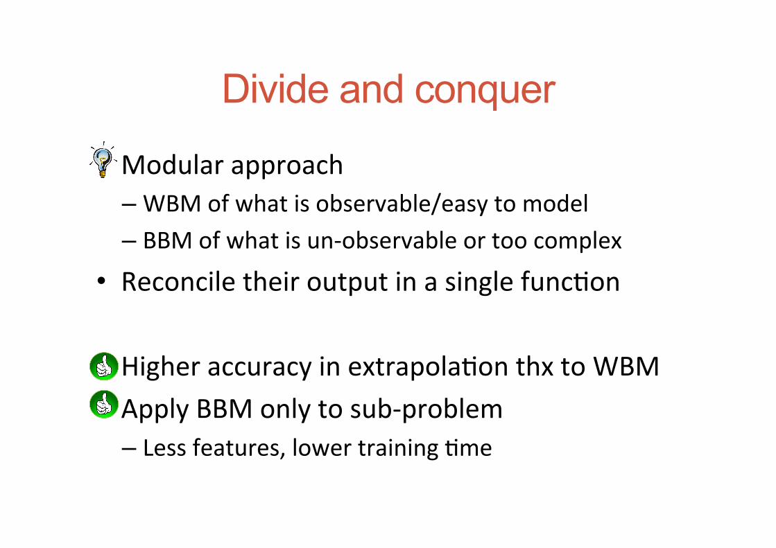
Divide and conquer

•  Modular approach – WBM of what is observable/easy to model – BBM of what is un-‐observable or too complex

•  Reconcile their output in a single func+on

•  Higher accuracy in extrapola+on thx to WBM •  Apply BBM only to sub-‐problem

– Less features, lower training +me

Case study: Infinispan

•  Distributed in-‐memory key-‐value store: – Nodes maintain elements of a dataset

•  Full vs par+al replica+on (# copies per item)

– Transac+onal -‐-‐ACI(D)– manipula+on of data •  Concurrency control scheme (enforce isola+on) •  Replica+on protocol (disseminate modifica+ons)

DTM optimization in the Cloud

•  Important to model network-‐bound ops but… •  Cloud hides detail about network L

– No topology info – No service demand info – Addi+onal overhead of virtualiza+on layer

•  BBM of network-‐bound ops performance – Train ML on the target pla_orm

TAS/PROMPT [TAAS14,Mascots14]

•  Analy+cal modeling (queuing theory based) –  Concurrency control scheme

•  E.g., encounter +me vs commit +me locking –  Replica+on protocol

•  E.g., PB vs 2PC –  Replica+on scheme

•  Par+al vs full –  CPU

•  Machine Learning –  Network bound op (prepare, remote gets) –  Decision tree regressor

Analytical model in TAS/PROMPT

•  Concurrency control scheme (lock-‐based) – A lock is a M/G/1 server –  Conflict prob = u+liza+on of the server

•  Replica+on protocol – mul+-‐master/Two-‐phase Commit based à one model –  single-‐master/primary-‐backup à two models

•  Replica+on scheme –  Probability of accessing remote data –  # nodes involved in commit

Machine Learning in TAS/PROMPT

•  Decision tree regressor •  Opera+on-‐specific models

– Latency during prepare – Latency to retrieve remote data

•  Input – Opera+ons rate (prepare, commit, remote get…) – Size of messages – # nodes involved in commit

ML accuracy for network bound ops

0

5000

10000

15000

20000

25000

30000

35000

0 5000 10000 15000 20000 25000 30000 35000

Pre

dic

ted T

pre

p(µ

sec)

Real Tprep(µsec)

EC2

500

1000

1500

2000

2500

3000

3500

4000

500 1000 1500 2000 2500 3000 3500 4000P

redic

ted T

pre

p(µ

sec)

Real Tprep(µsec)

Private Cluster

•  Seamlessly portable across infrastructures – Here, private cloud and Amazon EC2

AM and ML coupling

•  At training +me, all features are monitorable •  At query +me they are NOT!

EXAMPLE •  Current config: 5 nodes, full replica+on

– Contact all 5 nodes at commit

•  Query config: 10 nodes, par+al replica+on – How many contacted nodes at commit??

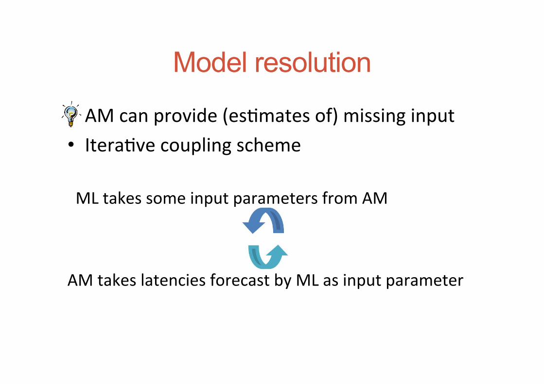
•  AM can provide (es+mates of) missing input •  Itera+ve coupling scheme ML takes some input parameters from AM

AM takes latencies forecast by ML as input parameter

Model resolution

Model’s accuracy

0.5

0.6

0.7

0.8

0.9

1

2 4 6 8 10 12 14 16 18 20

Co

mm

it P

rob

ab

ility

Number of nodes

EC2

TPCC-W-RealTPCC-W-Pred

TPCC-R-RealTPCC-R-Pred

0

500

1000

1500

2000

2500

3000

3500

4000

2 4 6 8 10 12 14 16 18 20

Th

rou

gh

pu

t (t

x/se

c)

Number of nodes

EC2



0.5

0.6

0.7

0.8

0.9

1

2 3 4 5 6 7 8 9 10

Com

mit

Pro

babili

ty

Number of nodes

PB, write transactions only



0

500

1000

1500

2000

2500

3000

3500

4000

4500

2 3 4 5 6 7 8 9 10

Th

rou

gh

pu

t (t

x/se

c)

Number of nodes




0

500

1000

1500

2000

2500

3000

3500

4000

4500

2 3 4 5 6 7 8 9 10

Thro

ughput (t

x/se

c)

Number of nodes




TOP: primary-‐backup. BOTTOM: mul+-‐master (2PC-‐based)

Comparison with Pure ML, I

•  YCSB (transac+fied) workloads while varying –  # opera+ons/tx –  Transac+onal mix –  Scale –  Replica+on degree

0

0.1

0.2

0.3

0.4

0.5

0.6

0.7

0 20 40 60 80

Me

an

re

lativ

e e

rro

r

Percentage of additional training set

CubistM5R

SMORegMLP

PROMPTDivide et Impera

Comparison with Pure ML, II

•  ML trained with TPCC-‐R and queried for TPCC-‐W •  Pure ML blunders when faced with new workloads

0

500

1000

1500

2000

2500

3000

3500

4000

2 4 6 8 10 12 14 16 18 20

Th

rou

gh

pu

t (t

x/se

c)

Number of nodes

real TAS pure ML

Gray box modeling


Hybrid ensembling


Bootstrapping

•  Obtain zero-‐training-‐+me ML via ini+al AM 1.  Ini+al (synthe+c) training set of ML from AM 2.  Retrain periodically with “real” samples

Analytical !model!

Boostrapping"training set!

Machine learning!!

Gray box "model!

Sampling of"the Parameter Space!

Model construction!

Current training set!

Machine learning!

Gray box "model!

New data"come in!

(1) (2)

How many synthetic samples?

0

0.1

0.2

0.3

0.4

0.5

0.6

0.7

2000 4000 6000 8000 10000 12000 14000 0.01

0.1

1

10

100

1000

10000

MA

PE

Tra

inin

g tim

e (

sec,

logsc

ale

)

Training set size

KVS-MAPEKVS-time

TOB-MAPETOB-time

•  Important tradeoff –  Higher # à lower fimng error over the AM output –  Lower # à higher density of real samples in dataset

How to update the synthetic training set?

•  Merge: simply add real samples to synthe+c set

•  Replace only the nearest neighbor (RNN)

•  Replace neighbors in a given region (RNR) – Two variants

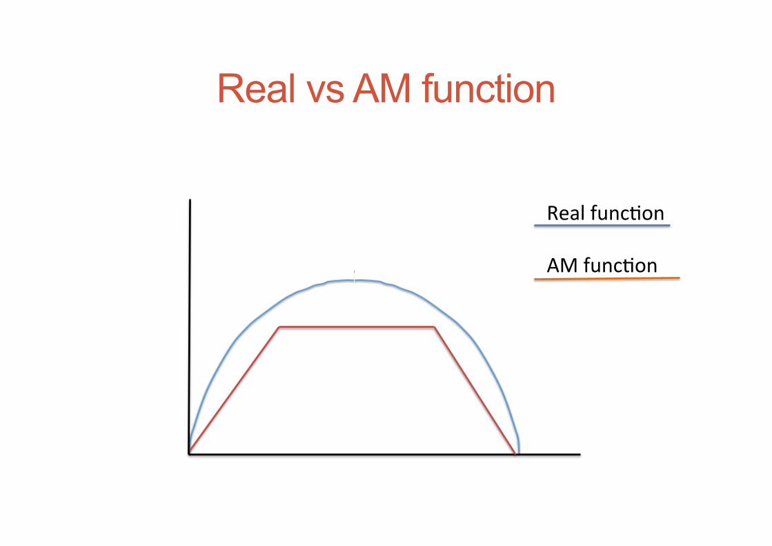
Real vs AM function

Real func+on AM func+on

•  Assuming enough point to perfectly learn AM

Real vs learnt

Synthe+c sample

ML func+on

•  Add real samples to synthe+c

Merge

Real sample

•  Problem: same/near samples have diff. output

Merge

•  Remove nearest neighbor

Replace Nearest Neighbor (RNN)

•  Preserve distribu+on…


•  … but may induce alterna+ng outputs


•  Add real and remove synth. samples in a radius

Replace Nearest Region (RNR)

•  R = radius defining neighborhood


R

•  R = radius defining neighborhood


R

•  Skew samples’ distribu+on


•  Replace all synthe+c samples in a radius R

Replace Nearest Region 2 (RNR2)

R

Replace Nearest Region 2 (RNR2)

•  Maintain distribu+on, piecewise approxima+on

Weighting

•  Give more relevance to some samples

•  Fit beoer the model around real samples – “Trust” real samples more than synthe+c ones – Useful especially in Merge

•  Too high can cause over-‐fimng! – Learner fails to generalize

Evaluation

•  Case studies – Response +me in Total Order Broadcast (TOB)

•  building block at the basis of many DTM •  2-‐dimensional yet highly nonlinear perf. Func+on

– Throughput in Distributed TM (Infinispan) •  7-‐dimensional performance func+on

Weighting

TOB (10K synthe+c samples)

154 CHAPTER 5. THE HYBRID ENSEMBLE APPROACH

0

0.1

0.2

0.3

0.4

0.5

1 2 5 10 100 1000Weight (log)

Merge 20

0

0.1

0.2

0.3

0.4

0.5

1 2 5 10 100 1000Weight (log)

Merge 70

0

0.1

0.2

0.3

0.4

0.5

1 2 5 10 100 1000

MA

PE

Weight (log)

BBM 20

0

0.1

0.2

0.3

0.4

0.5

1 2 5 10 100 1000

MA

PE

Weight (log)

BBM70

0

0.1

0.2

0.3

0.4

0.5

1 2 5 10 100 1000

MA

PE

Weight (log)

WBM

0

0.1

0.2

0.3

0.4

0.5

1 2 5 10 100 1000

MA

PE

Weight (log)

(a) TOB: 1K synthetic samples

0

0.1

0.2

0.3

0.4

0.5

1 2 5 10 100 1000M

AP

EWeight (log)

(b) TOB: 10K synthetic samples

0.1

0.2

0.3

0.4

0.5

1 2 5 10 100 1000

MA

PE

Weight (log)

(c) DTP: 1K synthetic samples

0.1

0.2

0.3

0.4

0.5

1 2 5 10 100 1000

MA

PE

Weight (log)

(d) DTP: 10K synthetic samples

Figure 5.5: Impact of the weight parameter for the Merge updating policy, using 1K and 10Ksynthetic samples.

accuracy for the DTP case. This arguably depends on the fact that Cubist approximates non-

linear functions by means of piece-wise linear approximation in the leaves of the decision tree

that it builds. Such model may be unable to properly approximate the performance function of

the base DTP performance model, which is defined over a multi-dimensional space and exhibits

strongly non-linear behaviors.

5.4.2.2 Updating

This section evaluates the alternative algorithms for the updating of the knowledge base, that

have been presented in Section 5.2.1.2: it first assesses the sensitivity of each algorithm to its key

parameters and finally compares their accuracy assuming an optimal tuning of such parameters.


0

0.1

0.2

0.3

0.4

0.5

1 2 5 10 100 1000Weight (log)

Merge 20

0

0.1

0.2

0.3

0.4

0.5

1 2 5 10 100 1000Weight (log)

Merge 70

0

0.1

0.2

0.3

0.4

0.5

1 2 5 10 100 1000

MA

PE

Weight (log)

BBM 20

0

0.1

0.2

0.3

0.4

0.5

1 2 5 10 100 1000

MA

PE

Weight (log)

BBM70

0

0.1

0.2

0.3

0.4

0.5

1 2 5 10 100 1000

MA

PE

Weight (log)

WBM

0

0.1

0.2

0.3

0.4

0.5

1 2 5 10 100 1000

MA

PE

Weight (log)


0

0.1

0.2

0.3

0.4

0.5

1 2 5 10 100 1000

MA

PE

Weight (log)


0.1

0.2

0.3

0.4

0.5

1 2 5 10 100 1000

MA

PE

Weight (log)


0.1

0.2

0.3

0.4

0.5

1 2 5 10 100 1000

MA

PE

Weight (log)








5.4.2.2 Updating





0

0.1

0.2

0.3

0.4

0.5

1 2 5 10 100 1000Weight (log)

Merge 20

0

0.1

0.2

0.3

0.4

0.5

1 2 5 10 100 1000Weight (log)

Merge 70

0

0.1

0.2

0.3

0.4

0.5

1 2 5 10 100 1000

MA

PE

Weight (log)

BBM 20

0

0.1

0.2

0.3

0.4

0.5

1 2 5 10 100 1000

MA

PE

Weight (log)

BBM70

0

0.1

0.2

0.3

0.4

0.5

1 2 5 10 100 1000

MA

PE

Weight (log)

WBM

0

0.1

0.2

0.3

0.4

0.5

1 2 5 10 100 1000

MA

PE

Weight (log)


0

0.1

0.2

0.3

0.4

0.5

1 2 5 10 100 1000

MA

PE

Weight (log)


0.1

0.2

0.3

0.4

0.5

1 2 5 10 100 1000

MA

PE

Weight (log)


0.1

0.2

0.3

0.4

0.5

1 2 5 10 100 1000

MA

PE

Weight (log)








5.4.2.2 Updating




DTM (10K synthe+c samples)

Update function

•  In both considered case studies, simplicity pays off: –  the Merge policy performs analogously to RNR2 –  …but, unlike RNR2, Merge is parameter-‐free

5.4. EVALUATION 159

0.2

0.3

0.4

0.5

10 20 30 40 50 60 70 80 90

MA

PE

% Training set

Merge

0.2

0.3

0.4

0.5

10 20 30 40 50 60 70 80 90

MA

PE

% Training set

RNR2-0.01

0

0.1

0.2

0.3

0.4

0.5

1 2 5 10 100 1000M

AP

EWeight (log)

WBM

0

0.1

0.2

0.3

0.4

0.5

1 2 5 10 100 1000

MA

PE

Weight (log)

BBM

0.1

0.2

0.3

0.4

0.5

0.6

0.7

0.8

10 20 30 40 50 60 70 80 90

MA

PE

% Training set

(a) TOB

0.2

0.3

0.4

0.5

10 20 30 40 50 60 70 80 90

MA

PE

% Training set

(b) DTP

Figure 5.7: Comparison between Merge and Replace-based Bootstrapping

The plot in Figure 5.7 clearly highlights the advantages that the Bootstrapping technique can

provide, eventually outperforming both the base model and the reference ML-based predictor.

It also shows that, in the considered case studies, and for the considered parameters’ values,

there is no clear winner between the two updating variants. In fact, the conducted evaluation

suggests —maybe surprisingly— that the weighting parameter results to be the one that affects

accuracy the most, up to the point that its careful tuning allows the Merge updating policy to

perform similarly to the —relatively more complex— RNR2.

5.4.2.3 Bootstrapping in extrapolation

So far, the Bootstrapping technique has been evaluated by drawing the additional training set Dt

for the black box learner uniformly at random from a real data set D, and assessing its accuracy

over D\Dt . This means that the learned performance function has been corrected by benefiting

from an unbiased sampling of the whole space over which its accuracy is then assessed. This

section serves the purpose of assessing the Bootstrapping technique’s robustness against biased

sampling strategies: even if provided only with a set R of real samples corresponding to narrow

regions of the parameters’ space, the bootstrapped learner still inherits the predictive power of

the base base predictor when working in extrapolation with respect to R.

A realistic use case for such a scenario would be if the real samples were not to be collected

Visualizing the correction BASE MODEL PURE ML (70% TS)

BOOTSTRAPPED ML (70% TS)

Gray box modeling


Hybrid ensembling


Hybrid KNN

Hybrid boos+ng Probing

Hybrid Boosting

•  Learning the error of a model on a func+on may be simpler than learning the func+on itself

•  Chain composed by AM + cascade of ML

•  ML1 trained over residual error of AM

•  MLi, i>1 trained over residual error of MLi-‐1

Training and Querying Hyboost

<x1, y1> <x2, y2> . . . <xn, yn>

Original training set

Training


<x1, y1> <x2, y2> . . . <xn, yn>

<x1, y1-‐ AM(x1)> <x2, y2 -‐ AM(x2)> . . . <xn, yn – AM(xn)>

Residual error of AM Original training set

AM

Training


<x1, y1> <x2, y2> . . . <xn, yn>


<x1, y1-‐ ML1(x1)> <x2, y2 – ML1(x2)>

.

.

. <xn, yn – ML1(xn)>

ML1

Residual error of AM Residual error of ML1 Original training set

AM

Training


<x1, y1> <x2, y2> . . . <xn, yn>


<x1, y1-‐ ML1(x1)> <x2, y2 – ML1(x2)>

.

.

. <xn, yn – ML1(xn)>

ML1

Residual error of AM Residual error of ML1

Query F(x) = AM(x) + ML1(x)+…+MLm(x)


AM

Training

Gray box modeling


Hybrid ensembling


Hybrid KNN


Hybrid KNN •  Predict performance of x with model that is supposed to be the most accurate for it

•  Split training set D into D’, D’’

•  Train ML1…MLN on D’ – ML can differ in nature, parameters, training set…

•  For a query sample z –  Pick the K training samples in D’’ closer to z –  Find the model with lowest error on the K samples – Use such model to predict f(x)

KNN Training and Querying

TR TRAINING SET ML1 MLn … AM


TR

ML TRAINING SET

KNN TRAINING SET

ML1 MLn … AM

TRAINING


TR

ML TRAINING SET

KNN TRAINING SET

ML1 MLn … AM

QUERYING

KNN, CUT-‐OFF C NEAREST NEIGHBORS

X


TR

ML TRAINING SET

KNN TRAINING SET

ML1 MLn … AM

QUERYING


EVALUATE ACCURACY

X


TR

ML TRAINING SET

KNN TRAINING SET

ML1 MLn … AM

QUERYING


EVALUATE ACCURACY

X MOST

ACCURATE MODEL


TR

ML TRAINING SET

KNN TRAINING SET

ML1 MLn … AM

QUERYING


EVALUATE ACCURACY

X MOST

ACCURATE MODEL

F(X)

Gray box modeling


Hybrid ensembling


Hybrid KNN


Probing •  Build a ML model as specialized as possible

– Use AM where it is accurate – Train ML only where AM fails

•  Differences w.r.t. KNN – Training: in KNN, ML is trained on all samples:

•  Here, ML trained on samples for which AM is inaccurate

– Querying: In KNN, vo+ng decides on ML vs AM •  Here, binary classifier predicts when the AM is inaccurate

Probing training and querying

<x1, y1> <x2, y2> . . . <xn, yn>


AM

ML training set Classifier training set

TRAINING

Probing training and querying Original training set

AM


<x1, y1>

TRAINING

ERROR < CUT-‐OFF?


AM


ERROR < CUT-‐OFF?

<x1, y1>

YES

<x1, AM>

TRAINING


AM


<x2, y2>

NO

<x1, AM>

<x2, ML>

NO

<x2, y2>

ERROR < CUT-‐OFF?

TRAINING

Probing training and querying

ML

QUERYING

CLASSIFIER AM

x

F(x) = AM(x) if Classify(x) = AM ML(x) otherwise

Evaluation

•  Sensi+vity to meta-‐parameters – Hyboost

•  Size of the chain – Hybrid KNN

•  Proximity cut-‐off – Probing

•  Minimum AM’s accuracy cut-‐off

•  Comparison among the techniques

HyBoost

•  Chain composed by AM + Decision Tree •  Longer chains yielded negligible improvements in the considered case studies

5.4. EVALUATION 161

0

0.1

0.2

0.3

0.4

0.5

1 2 5 10 100 1000

MA

PE

Weight (log)

WBM

0

0.1

0.2

0.3

0.4

0.5

1 2 5 10 100 1000

MA

PE

Weight (log)

BBM

0.1

0.2

0.3

0.4

0.5

0.6

0.7

0.8

10 20 30 40 50 60 70 80 90

MA

PE

% Training Set

HyBoost

0.1

0.2

0.3

0.4

0.5

0.6

0.7

0.8

10 20 30 40 50 60 70 80 90

MA

PE

% Training Set

(a) TOB

0.1

0.2

0.3

0.4

0.5

10 20 30 40 50 60 70 80 90

MA

PE

% Training Set

(b) DTP

Figure 5.9: Evaluating the accuracy of HyBoost.

region.

Figure 5.8c, instead, shows the accuracy achieved by a bootstrapped learner trained over a

combination of synthetic samples and the same set of real samples used in the previous case.

Clearly, the accuracy in the right part of the plot is similar to the one in Figure 5.8b; the left part,

instead, which corresponds to the performance queries in extrapolation, portrays a significant

enhancement in accuracy. These improved predictive capabilities in extrapolation stem from the

availability of a synthetic training set provided by the embedded base model. This claim can be

verified by analyzing Figure 5.8a, which reports the accuracy of a Cubist learner trained only

over synthetic data samples: it is easy to see that the left side of the plot is very similar to the

left side of the plot in Figure 5.8b, demonstrating how a bootstrapped learner is able to leverage

the knowledge provided by the base model about the performance of the target application in

unexplored regions of the parameters’ space.

5.4.3 Hybrid Boosting

The conducted evaluation study on the HyBoost technique, described in this section, only fo-

cuses on analyzing the effectiveness of this technique depending on the characteristics of the

white and black box models for two considered case studies. The only tuning parameter of

this technique, in fact, would be the size and the composition of the chain, i.e., the number of

Infinispan

Tuning of hyper-parameters matters

•  Comparison – Pure AM, Pure ML (Cubist, Decision tree regressor) vs – Probing (AM + Cubist)

•  Analogous considera+ons hold for KNN

5.4. EVALUATION 165

0.1

0.2

0.3

0.01 0.2 0.4 0.6 0.8 1

MA

PE

Cutoff

PROB 60

0.1

0.2

0.3

0.01 0.2 0.4 0.6 0.8 1

MA

PE

Cutoff

PROB 80 0.2

0.3

0.4

0.5

0.01 0.2 0.4 0.6 0.8 1M

AP

E

Cutoff

PROB 40

0.2

0.3

0.4

0.5

0.01 0.2 0.4 0.6 0.8 1M

AP

ECutoff

PROB 20

0

0.1

0.2

0.3

0.4

0.5

1 2 5 10 100 1000

MA

PE

Weight (log)

BBM 20

0

0.1

0.2

0.3

0.4

0.5

1 2 5 10 100 1000M

AP

EWeight (log)

WBM

0.1

0.2

0.3

0.4

0.5

0.01 0.2 0.4 0.6 0.8 1

MA

PE

Cutoff

BBM 40

0.1

0.2

0.3

0.01 0.2 0.4 0.6 0.8 1

MA

PE

Cutoff

BBM 60 BBM 80

0.1

0.2

0.3

0.01 0.2 0.4 0.6 0.8 1

MA

PE

Cutoff

BBM 60 BBM 80

0.2

0.3

0.4

0.5

0.01 0.2 0.4 0.6 0.8 1

MA

PE

Cutoff

(a) 20% and 40% of training set

0.1

0.2

0.3

0.01 0.2 0.4 0.6 0.8 1

MA

PE

Cutoff

(b) 60% and 80% of training set

Figure 5.12: Sensitivity analysis of Probing w.r.t. the c parameter (TOB)

prediction as accurate. The classification algorithm employed to train the classifier responsible

for estimating the best model for a given query is the Weka implementation of the C.45 Decision

Tree (Quinlan, 1993b).

Figure 5.12 and Figure 5.13 report the results of such sensitivity analysis. The first phe-

nomenon that comes evident for both the case studies is that the accuracy does not vary, as a

function of c, as smoothly as in the KNN case, which is the other considered Selection-based

Hybrid Ensemble technique that relies on a cutoff parameter. This is because c directly affects

both the training set of the classifier used and of the black box performance predictor. The

resulting behavior of these two components affects in an intertwined and complex fashion that

ultimately results in the portrayed accuracy trends.

Also, as expectable, for both case studies, the lower the employed cut-off value the more

the accuracy is similar to the one attained by the black box model. This happens because the

underlying white box model is considered to be accurate and, thus, to be reliable, only if it

attains a correspondingly low error. In a dual fashion, as c moves towards higher values, the

accuracy delivered by the Probing-based predictor resembles the underlying base model’s one.

Regarding the specific case studies, the characteristics of the corresponding base predic-

tors and black box models play again a fundamental role to determine the effectiveness of the


0.2

0.3

0.4

0.5

0.01 0.2 0.4 0.6 0.8 1

MA

PE

Cutoff

(a) 20% and 40% of training set

0.2

0.3

0.01 0.2 0.4 0.6 0.8 1

MA

PE

Cutoff

(b) 60% and 80% of training set

Figure 5.13: Sensitivity analysis of Probing w.r.t. the c parameter (DTP)

Probing technique. In the TOB case, in fact, Probing only slightly enhances the accuracy with

respect to the best between the pure white and black approaches at a medium training set (Fig-

ure 5.12a). With lower training set, the classifier cannot distinguish when it is better to rely

on the white or the black box. At higher training sets, the accuracy of the black box model

alone is generally better than its white box counterpart’s (Figure 5.12b). As a result, even if the

accuracy of the white box model is below the desired threshold, it is likely that the black box

learner alone could still reach a higher accuracy, if trained with the proper data-set. Ultimately,

this leads the Probing-based predictor to rely on the white box model even when it should not,

and in removing samples from the black box learner’s training set, thus reducing its accuracy.

The plots in Figure 5.13, instead, reveal slightly different dynamics for what concerns the

DTP case study. On one side, in fact, just like the TOB case, the classifier does not help, or only

marginally helps, in increasing accuracy when there is low amount of training data available

(Figure 5.13a. Conversely, as training data become more abundant, Probing is able to deliver

higher accuracy than the two underlying models alone (Figure 5.13b) this is because, as already

highlighted during the KNN discussion, there is no clear winner between the white and the

black box model. Therefore, provided that the classifier is able to distinguish when to prefer

one over the other, it is possible to take selectively advantage of both with beneficial effects on

accuracy.

No free lunch theorem strikes again

•  No one-‐size-‐fits-‐all hybrid model exists •  Tackle choice of best hybrid model via cross-‐valida+on

5.4. EVALUATION 167

0.1

0.2

0.3

0.4

20 40 60 80

MA

PE

% Training Set

BBM

WBM

Bootstrapping

HyBoost

Probing

KNN

0.1

0.2

0.3

0.4

20 40 60 80

MA

PE

% Training Set

BBM

WBM

Bootstrapping

HyBoost

Probing

KNN

0.1

0.2

0.3

0.4

20 40 60 80

MA

PE

% Training Set

BBMWBM

BootstrappingHyBoost

ProbingKNN

0.1

0.2

0.3

0.4

20 40 60 80M

AP

E% Training Set

BBM

0.1

0.2

0.3

0.4

20 40 60 80

MA

PE

% Training Set

BBMWBM

BootstrappingHyBoost

ProbingKNN

0.1

0.2

0.3

0.4

20 40 60 80

MA

PE

% Training Set

WBMBootstrapping

HyBoostProbing

KNN

0.1

0.2

0.3

0.4

20 40 60 80

MA

PE

% Training Set

(a) TOB

0.1

0.2

0.3

0.4

20 40 60 80

MA

PE

% Training Set

(b) DTP

Figure 5.14: Comparing the performance of the 4 proposed gray box techniques.

5.4.6 Comparison among the approaches

This section concludes the experimental evaluation and is dedicated to comparing the accuracy

achieved by the four proposed hybrid ensemble techniques in the two considered case studies.

In particular, the comparison is performed assuming a proper tuning of the internal parameters

of the compared ensemble algorithms. Specifically, the reported data are obtained using 10-fold

cross validation to determine appropriate values for the internal parameters of the compared

ensemble algorithms.

As already hinted in Section 5.4.1.3, identifying the best gray box model and correspond-

ing parameterization given some training data is a problem that falls beyond the scope of the

proposed Hybrid Ensemble techniques: it is, indeed, a common trait shared with pure black box

modeling techniques. Therefore, it can be tackled by means of standard techniques developed

for the selection and tuning of Machine Learning algorithms, such as Bayesian Optimization or

grid/random search (Bergstra et al., 2011).

The following evaluation aims at showing how the characteristics of the target performance

function and of a hybrid predictor affect accuracy in the most favorable case, i.e., excluding

the cases in which a given predictor performs poorly only because of a correspondingly poor

setting of its internal parameters.

Figure 5.14 reports the accuracy attained by the four proposed gray box models, as well as

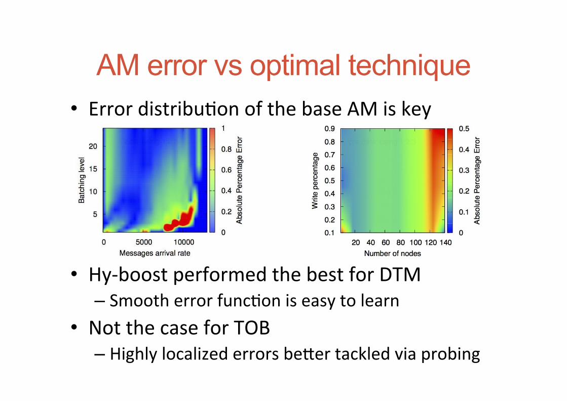
AM error vs optimal technique •  Error distribu+on of the base AM is key

•  Hy-‐boost performed the best for DTM – Smooth error func+on is easy to learn

•  Not the case for TOB – Highly localized errors beoer tackled via probing

Concluding remarks: TM and Self-tuning

•  Transac+onal memory is an aorac+ve alterna+ve to lock-‐based synchroniza+on: –  hides complexity behind intui+ve abstrac+on –  relevance amplified by integra+on with GCC, commodity (Intel’s) and HPC (IBM’s) CPUs

•  Performance of TM is strongly affected by: – workload characteris+cs –  choice of the TM implementa+on –  plethora of implementa+on-‐dependent parameters

•  Self-‐tuning is cri+cal to ensure efficiency!

Concluding remarks: Which modeling methodology?

•  White and black box models can be effec+vely used in synergy –  Increased predic+ve power via analy+cal models –  Incremental learning capabili+es via black box models

•  Presented three gray box methodologies: – Divide and conquer, Bootstrapping, Hybrid ensembling – Design, implementa+on and applica+on to (D)TM

•  Careful choice of technique and parameters – Use standard techniques for hyper-‐parameters opt.

Open questions

•  Any other way of hybridizing Black and White modelling?

•  Can we further combine them? •  e.g. use a bootstrapped model in

an ensemble? •  Can we infer the best gray box

technique by analyzing the error func+on of the AM model?

References •  [SPAA08] Torvald Riegel, Christof Fetzer, Pascal Felber, Automatic data partitioning in

software transactional memories. SPAA 2008: 152-159 •  [PPoPP08] Pascal Felber, Christof Fetzer, Torvald Riegel, Dynamic performance tuning of word-based

software transactional memory. PPOPP 2008: 237-246 •  [SASO12] D. Didona, D. Carnevale Paolo Romano, S. Galeani, An Extremum Seeking Algorithm for

Message Batching in Total Order Protocols, IEEE International Conference on Self-Adaptive and Self-Organizing Systems (SASO 2012), Lyon, France, 10-14 Sept. 2012

•  [Netys13] Diego Didona, Pascal Felber, Derin Harmanci, Paolo Romano and Joerg Schenker, Identifying the Optimal Level of Parallelism in Transactional Memory Systems, The International Conference on Networked Systems 2013, BEST PAPER AWARD

•  [DSN13] M. Couceiro, P. Ruivo, Paolo Romano, L. Rodrigues, Chasing the Optimum in Replicated In-memory Transactional Platforms via Protocol Adaptation, The 43rd Annual IEEE/IFIP International Conference on Dependable Systems and Networks (DSN 2013)

•  [ICAC 13] Joao Paiva, Pedro Ruivo, Paolo Romano and Luis Rodrigues, AutoPlacer: scalable self-tuning data placement in distributed key-value stores, The 10th International Conference on Autonomic Computing (ICAC 2013), San Jose, CA, USA, 26-28 June 2013 - BEST PAPER AWARD FINALIST

•  [PACT14] N. Diegues and Paolo Romano and L. Rodrigues, Virtues and Limitations of Commodity Hardware Transactional Memory, The 23rd International Conference on Parallel Architectures and Compilation Techniques (PACT 2014), August 2014

•  [JPDC14] M. Castro et al., Adaptive thread mapping strategies for transactional memory applications, Journal of Parallel and Distributed Computing, Volume 74, Issue 9, September 2014

•  [TAAS14] D. Didona, Paolo Romano, S. Peluso, F. Quaglia, Transactional Auto Scaler: Elastic Scaling of In-Memory Transactional Data Grids, ACM Transactions on Autonomous and Adaptive Systems (TAAS), 9, 2, 2014

•  [ICPE15] D. Didona, Paolo Romano, F. Quaglia, E. Torre, Combining Analytical Modeling and Machine-Learning to Enhance Robustness of Performance Prediction Models, 6th ACM/SPEC International Conference on Performance Engineering (ICPE), Feb 2015


THANK YOU

Ques+ons?

romano@inesc-‐id.pt www.gsd.inesc-‐id.pt/~romanop

Documents

Self%tuning+Transac1onal+Memory+ via+Machine+Learning++