Self-similarity and turbulence characteristics of wind turbine … Library/Our People/Profiles... · Self-similarity and turbulence characteristics of wind ... directly solving the

WIND ENERGYWind Energ. (2014)

Published online in Wiley Online Library (wileyonlinelibrary.com). DOI: 10.1002/we.1792

RESEARCH ARTICLE

Self-similarity and turbulence characteristics of windturbine wakes via large-eddy simulationShengbai Xie and Cristina ArcherCollege of Ocean, Earth and Environment, University of Delaware, Newark, Delaware 19716

ABSTRACT

Mean and turbulent properties of the wake generated by a single wind turbine are studied in this paper with a new largeeddy simulation (LES) code, the wind turbine and turbulence simulator (WiTTS hereafter). WiTTS uses a scale-dependentLagrangian dynamical model of the sub-grid shear stress and actuator lines to simulate the effects of the rotating blades.WiTTS is first tested by simulating neutral boundary layers without and with a wind turbine and then used to study thecommon assumptions of self-similarity and axisymmetry of the wake under neutral conditions for a variety of wind speedsand turbine properties. We find that the wind velocity deficit generally remains self similarity to a Gaussian distribution inthe horizontal. In the vertical, the Gaussian self-similarity is still valid in the upper part of the wake, but it breaks downin the region of the wake close to the ground. The horizontal expansion of the wake is always faster and greater than thevertical expansion under neutral stability due to wind shear and impact with the ground. Two modifications to existingequations for the mean velocity deficit and the maximum added turbulence intensity are proposed and successfully tested.The anisotropic wake expansion is taken into account in the modified model of the mean velocity deficit. Turbulent kineticenergy (TKE) budgets show that production and advection exceed dissipation and turbulent transport. The nacelle causessignificant increase of every term in the TKE budget in the near wake. In conclusion, WiTTS performs satisfactorily in therotor region of wind turbine wakes under neutral stability. Copyright © 2014 John Wiley & Sons, Ltd.

KEYWORDS

wind turbine wake; wake model; self-similarity; turbulence; large-eddy simulation

Correspondence

Shengbai Xie, College of Ocean, Earth and Environment, University of Delaware, Newark, Delaware 19716.E-mail: [email protected]

Received 22 August 2013; Revised 5 July 2014; Accepted 11 July 2014

1. INTRODUCTION

With the increasing demand for clean, safe and cheap energy, wind power has been expanding globally in recent yearsand it has become a dominant renewable energy source, with over 280 GW installed worldwide by the end of 2012.1 Ingeneral, wind turbines are installed in wind farms along several rows and columns. Because wind turbines generate wakesthat propagate downwind, the wakes from turbines in upwind rows can impact negatively the performance of downwindrows. Understanding wake losses is therefore an increasingly important topic as wind farms grow in size and in numberof turbine rows. Although a modern wind turbine can be very large in size, e.g. >100 m in both diameter and hub height,it still operates in the lower part of the atmospheric boundary layer (ABL hereafter), where the wind is highly turbulent.Therefore, it is important to study the interaction between the turbulent atmosphere and the wind turbine wake in order tooptimize the design of the wind turbine as well as the layout of the wind farm for maximum energy extraction.

As comprehensively reviewed in,2, 3 wind turbine wakes have been extensively studied in the past two decades. However,this topic is still far from being fully understood because of the highly turbulent nature of wakes. The wake can be roughlydivided into two regions: the near wake and the far wake (although sometimes a transition region is also considered2). Thenear wake region is where the effect of the rotor is dominant and the wake is significantly affected by blade aerodynamics,stalled flow and tip vortices.3 Tip vortices are shed from the blade tip and root and propagate a short distance downstreamfollowing helical trajectories. When the inclination angle is small, the tip vortices can be interpreted as cylindrical shearlayers that expand in the wake due to turbulent diffusion and forms a ring-shaped domain of high turbulence intensity andgreat velocity gradients.2 At a certain distance downstream, the tip vortices break down because of instability. This distance

Copyright © 2014 John Wiley & Sons, Ltd.

Self-similarity and turbulence of wind turbine wakes via LES S. Xie and C. Archer

marks the end of the near wake region.2 The range of the near wake region depends on wind loads and inflow conditions.Typically, it is confined to the region from the rotor to less than three diameters (D) downstream.4 Beyond the near wake,past a transitional region,2 the far wake region begins in which the wake is fully developed. Hypothetically, in the absenceof ambient wind shear, velocity and turbulence intensity should remain self-similar and axisymmetric. In this region, rotoreffects are less important, whereas turbulent diffusion of momentum becomes dominant. Most effort in the literature hasbeen put toward understanding the far wake behavior.3

The modeling frameworks to study wind turbine wakes can also be roughly divided into two groups: kinetic models andfield models.2, 3 In kinetic models, also known as explicit models, an analytical expression of a specific wake property, suchas wind speed deficit, is explicitly given. Most kinetic models are based of self-similarity.5–8 In some widely used wakemodels, e.g. WAsP, the Wind Atlas Analysis and Application Program,6, 9 the wake is assumed to be axisymmetric andgrows linearly with a constant velocity deficit through the wake radius, whereas the deficit decays with distance followinga power law. However, the self-similarity and axisymmetry assumptions are questionable in the presence of strong windshear and ground effects3, 5, 10 and will be therefore evaluated in this study. Kinetic models have achieved great success inthe wind industry sector due to their simplicity and computer efficiency.

The second approach to studying wind turbine wakes is to use so-called field models, also known as implicit models,which solve the flow equations numerically at every point of the flow field. In early works, a linearized form of the momen-tum equation in the main flow direction was used together with a parabolic approximation, a constant advection velocityand a constant eddy viscosity.11 Ainslie12 developed a parabolic eddy viscosity model in which the wake was assumedto be axisymmetric. Because of the improvements in computer power, efficiency and cost, numerical modeling of windturbine wakes using computation fluid dynamics (CFD) has become more popular in recent years.10, 13–18

So far, directly solving the flow interactions with the blades at high Reynolds numbers has been too computationallyintensive for most practical applications, especially if multiple wind turbines are considered. Therefore, parameterizationsof the aerodynamic forces on the rotor have been developed in the wind industry community. An example of such aparameterization is the actuator disk model, which uses a permeable circular disk to represent the rotor, and the integratedthrust force induced by the wind turbine is uniformly distributed on the disk.3, 14 This approach is easy to implement intoa classic unsteady Navier–Stokes solver and has shown satisfactory results with relatively coarse grids.19, 20 However, theoriginal disk models were not able to take into account the rotational effects of the wind turbine blades since only drag forcealong the axial direction was considered. Alternatively, the actuator line model10, 15, 17 calculates the instantaneous dragand lift forces of each blade element from tabulated airfoil data and distributes the forces along actuator lines representingthe blades. Since the actuator line model uses the aerodynamic information of each blade element, it is capable of capturingdetailed three-dimensional (3D) rotational phenomena, such as tip vortices, and it is therefore used in this study. Thedisadvantage is that both finer grid resolution and smaller time steps are required by the actuator line model than by theactuator disk model to smoothly resolve the flow structures that form on the fast moving blade tips.

Another important issue in using CFD for studying wind turbine wakes is how to properly represent the ABL turbulence.As pointed out by Chamorro and Porté-Agel21 from their wind tunnel measurements, the turbulence properties of theincoming ABL have significant effects on the wakes. Since the Reynolds number of such a flow is usually very high (> 107

based on rotor diameter and free wind speed at hub height), direct numerical simulation is still practically impossiblewith today’s computer technology. Consequently, assumptions and simplified cases have been often used. In early CFDstudies of wind turbine wakes, laminar free-stream flow with uniform wind speed has been widely used.13, 16, 17 Troldborget al.22 generated a turbulent inflow with the same spectral characteristics as the real atmosphere by exerting time-varyingbody forces in a plane upstream the rotor but without mean wind shear. The techniques of solving Reynolds averagedNavier–Stokes equations are powerful in the study of high Reynolds number problems, and their relatively high efficiencyis attractive from the industry point of view. Crespo et al.2, 4, 23 developed the UPMWAKE model to calculate the windturbine wake in the ABL using a parabolic approximation and the � � � model for turbulence closure. However, Reynoldsaveraged Navier–Stokes models directly resolve only the mean flow properties and parameterize the effects of the Reynoldsstresses, whereas large eddy simulation (LES) models directly resolve the unsteady flow properties, not the mean flowproperties, all the way down to the filter scale and parameterize the effects of eddies smaller than that scale with theso-called sub-grid scale (SGS) models. Consequently, LES has become increasingly popular for ABL simulations in recentyears.24, 25 Jimenez et al.14 used a classic dynamic SGS model26 to show that LES can be used successfully to investigatethe details of the flow within wind turbine wakes. Calaf et al.19, 20 studied the fully developed, neutral boundary layer inan array of several wind turbines using LES with a scale-dependent Lagrangian SGS model.25, 27, 28 This SGS model isparticularly suitable to study the anisotropic turbulence with complex geometry, such as wind turbine wakes, since it doesnot need any spatial averaging. The same SGS model was also used in Lu and Porté-Agel’s15 study of a large wind farm ina stable ABL and will be used in this study as well.

In this paper, a new LES code is developed to study wind turbine wakes, the wind turbine and turbulence simulator(WiTTS), which uses the scale-dependent Lagrangian model for the SGS stresses and an actuator line model for the windturbine rotor. By using WiTTS, the assumption of self-similarity and several wake models is examined for a single windturbine in a neutral ABL. Turbulence intensity and TKE budgets are also studied. The paper is organized as follows. WiTTS

Wind Energ. (2014) © 2014 John Wiley & Sons, Ltd.DOI: 10.1002/we

S. Xie and C. Archer Self-similarity and turbulence of wind turbine wakes via LES

is introduced in Section 2; details of the simulation setup are given in Section 3; the WiTTS validation is presented inSection 4; and results of both mean flow properties and turbulence properties are discussed in Section 5.

2. WITTS: NUMERICAL METHODS AND MODELING APPROACHES

2.1. Governing equations and discretization

In this study, the filtered incompressible Navier–Stokes equations

@Qui

@tC Quj

@Qui

@xjD �

1

�

@Qp

@xi�@� r

ij

@xjC f�i �…ıi1 (1)

with the continuity constraint

@Qui

@xiD 0 (2)

are solved by LES. Here, i D 1, 2, 3; Qui is the filtered fluid velocity; � rij is the trace-free part of the SGS stress tensor;

Qp is the filtered modified dynamic pressure including the trace of the SGS stress tensor, � is air density and f�i is thebody-forcing term from the actuator line model. The SGS stress tensor � r

ij is modeled by a scale-dependent Lagrangiandynamic model,25, 27 discussed later in Section 2.2, and the flow is driven by a streamwise pressure gradient …. For astatistically steady and fully developed flow,

… D �u2�

H(3)

where H is the height of the computational domain, u� is the prescribed friction velocity. The air density � is assumed tobe constant in this study and the molecular viscosity is neglected since the Reynolds number is sufficiently high. However,since the molecular viscous effect is important near the wall, a wall model is needed to calculate the wall shear stresscorrectly, which will be described later in Section 2.2.

Equations (1) and (2) are solved by finite difference schemes discretisized on a marker-and-cell staggered grid.29 Theadvective term A D Quj@Qui=@xj at time step n is calculated by a hybrid method combining the fourth-order WeightedEssentially non-oscillatory (WENO) scheme30 and a conserved the fourth-order central scheme,31 i.e.

An D ˛.An/central C .1 � ˛/.An/WENO (4)

where ˛ < 1 is a weighting function that is set to be 0.8 in this study. The hybrid scheme is proposed because the centralscheme induces numerical oscillations where the velocity gradient is large, meanwhile, the WENO scheme can suppressthe non-physical oscillations but is found to be too dissipative in calculating turbulence fluctuations.

Equations (1) are marched in time by a fractional step method.32 First, the momentum equation without thepressure term is integrated in time explicitly then a Poisson equation is solved to update pressure satisfying the continuityconstraint (Equation (2)). In this study, a paralleled multigrid approach with red-black Gauss–Seidel smoother is used asthe Poisson solver.33

2.2. Scale-dependent Lagrangian dynamic model of SGS shear stress

In a LES, a parametrization is required for the closure of the system of equations. The linear eddy viscosity model is widelyused to relate the deviatoric part of the SGS stress tensor to the filtered rate of strain tensor

� rij D �2�r QSij (5)

where �r is the eddy viscosity for SGS motions, and QSij is the resolved strain rate tensor

QSij D1

2

�@Qui

@xjC@Quj

@xi

�(6)

The Smagorinsky model34 is often used for eddy viscosity

�r D .CS4/2ˇ̌QSˇ̌

(7)



where CS is the Smagorinsky coefficient, generally assumed to be constant;35 4 is the filter width; andˇ̌QSˇ̌

is thecharacteristic filtered rate of strain defined by ˇ̌

QSˇ̌D�2QSij QSij

�1=2(8)

Since CS in reality varies in different flow regions, a dynamic approach is utilized to determine its value. This approach isbased on the Germano identity26

Lij D Qui Quj � Qui Quj D Tij � � ij (9)

where .�/ denotes a test filtering with filter width of4 D ˛4 and ˛ is usually taken as 2; Lij is the resolved stress; and Tij

is the SGS stress at the test filter scale. The Smagorinsky model is used for Tij as follows:

Tdij � Tij �

1

3Tkkıij D �2.CS˛4/

2ˇ̌̌QSˇ̌̌QSij (10)

where .�/d denotes the deviatoric part of a tensor. Next, Equations (5) and (10) are substituted into Equation (9) to get theerror

eij D Ldij � C2

S,4Mij (11)

where

Mij D 242�ˇ̌QSˇ̌QSij � ˛

2ˇˇ̌̌QSˇ̌̌QSij

�(12)

and

ˇ D C2S,˛4=C2

S,4 (13)

The parameter ˇ is the ratio between the coefficients at the test filter scale and at the filter scale. By minimization of the errorusing a least square approach36 and assuming that ˇ D 1, the Smagorinsky coefficient at the test filter scale is obtained as

C2S D

JLM

JLM, (14)

where J.�/ is an averaging process to eliminate numerical instability. For general inhomogeneous turbulence where a spatialaverage is problematic, Meneveau et al.28 developed a weighted Lagrangian time average along the fluid trajectory asfollows

JLM D

Z t

�1LijMijŒx.t0/, t0�W.t � t0/dt0 (15)

and

JLM D

Z t

�1MijMijŒx.t0/, t0�W.t � t0/dt0 (16)

where W.t� t0/ D .1=T/e.t�t0/=T is the weighting function and T is chosen as T D 1.54.JLMJMM/�1=8. The exponential

form of W.t � t0/ allows using forward relaxation-transport equations to replace the backward time integrals as follows

DJLM

DtD@JLM

@tC Qu � JLM D

1

T�.LijMij � JLM/ (17)

and

DJMM

DtD@JMM

@tC Qu � JMM D

1

T�.MijMij � JMM/ (18)

By using the first-order numerical time and space schemes, Equations (17) and (18) can be solved easily and economicallyto update JLM and JMM at each time steps.



The assumption of ˇ D 1 implies a scale invariance, i.e. C2S,4 D C2

S,˛4. However, this assumption is questionable andit was found that Cs obtained with Equation (14) corresponds to the test filter scale ˛4 rather than grid filter scale 4.27

Porté-Agel et al.25 and Bou-Zeid et al.27 introduced scale-dependent approaches by using the second test filter at scaleO4 D ˛24 to calculate ˇ dynamically. Following Bou-Zeid et al. approach, by applying the previously discussed Germano

identity and minimizing the error at the second test filter scale, the coefficient at this scale can be obtained as

C2S,˛24

DJQN

JNN(19)

and JQN ,JNN can be calculated in a similar way to Equations (17) and (18), where QN D QijNij, NN D NijNij and

Qij DbQui Quj� OQui OQuj, Nij D 242�1

ˇ̌QSˇ̌QSij � ˛

4ˇ2jbQSjbQSij

�. Assuming that ˇ is scale-invariant (this assumption is more reasonable

than the scale-invariant assumption of CS), such that ˇ D C2S,˛24

=C2S,˛4 D C2

S,˛4=C2S,4 implies that

C2S,4 D C2

S,˛4=ˇ DJLM=JMM�JQN=JMM

JNN=JLM

� (20)

The molecular viscous effect is important near the wall and it is taken into account by a local similarity model27

as follows:

�walli,3 .x, y/ D �w.x, y/

Qui.x, y,4z=2/qQu

21 C Qu

22

, i D 1, 2 (21)

where

�w.x, y/ D �

24 �

ln�4z=2

z0

�352 hQu1.x, y,4z=2/2 C Qu2.x, y,4z=2/2

i(22)

and z0 is the uniform surface roughness.

2.3. Actuator line model of wind turbine aerodynamics

In this study, the wind turbine blades are modeled by an actuator line model.17 This model treats each blade as an actuatorline which is comprised of a series of airfoil elements along the spanwise direction. At each element with a radius r in the.� , x/ plane where � is the azimuthal coordinate, as shown in Figure 1, the incident tangential velocity V� and the normalvelocity Vx are calculated by using an iterative blade element momentum (BEM) method.37 Note that in a standard actuatorline model, V� and Vx at the blade can be directly calculated from the velocity field by interpolation, so the BEM methodis not necessary. But in our simulations, we found that interpolating directly at the blade is a bit problematic since it usesvelocities affected by the distribution of the body forces. Instead, we interpolate the streamwise velocity a certain distanceupstream of the blade (about 3x), which is less affected by the rotor and then uses this velocity to predict the velocities atthe blade by the BEM method. The local relative velocity Vrel can be expressed as

Vrel D .V� �r, Vx/ (23)

where is the rotational speed of the turbine. Hence, the angle between Vrel and the rotor plane is � D tan�1.Vx=.r �V� //. The angle of attack is defined as ˛ D � � � , where � is the local pitch angle. The lift coefficient CL and thedrag coefficient CD are functions of ˛ and can be found from a tabulated data for a specific airfoil. Consequently, theaerodynamic force per spanwise unit length is calculated as

f DFdrD

1

2�V2

relc.CLeL C CDeD/ (24)

where � is the air density; c is the chord length; and eL, eD are the unit vectors in the directions of lift and drag, respectively.A 3D Gaussian distribution function17 is applied to spread f smoothly from each airfoil element to grid points in thefollowing convolution form

f� D f˝ � , � D1

�3�3=2exp

�

d2

�2

!(25)



Figure 1. Cross-section airfoil element.

where d is the distance between a grid point and the element at the actuator line; � is the regularization kernel; and � is aconstant to adjust the width of the distribution, which is set equal to the grid size in this study following Mikkelsen38 andWu and Porté-Agel.18 Previous studies have shown that the predicted power is sensitive to this value.10, 39 Churchfield etal.40 suggested that " D C=4.3 such that the Gaussian width is similar to the chord length C. Since the grid width D.xyz/

1=3 in this study is about half of the chord length, it means that " � =2. However, as shown by Troldborg,10 asmall value of " causes spurious oscillations in the resulting velocity field. In this study, we found that " D works wellby comparing our LES data to the wind tunnel measurements as shown in Section 4.2.

The nacelle can be taken into account as a drag force Fx

Fx D1

2�CD,nacAnacU2

hub (26)

where Anac is the incident area of the nacelle, and CD,nac is the drag coefficient of the nacelle. The tower of the wind turbinecan also be modeled as a drag force. However, it is neglected because of its small size compared with the resolution usedin the current numerical simulations.

3. SIMULATION SETUP

The WiTTS model is used to study the neutrally stratified turbulent boundary layer with a single wind turbine above a flatground surface. In this study, the simulation setup generally follows the boundary layer wind tunnel tests of Saint AnthonyFalls Laboratory at the University of Minnesota.21 The streamwise length of the computational domain is Lx D 4.32 m,the vertical height is Lz D 0.46 m and the spanwise length is Ly D 0.72 m (Figure 2). The wind turbine is located0.6 m downstream from the inlet section and at the center in the spanwise direction. The diameter of the turbine rotoris D D 0.15 m and the hub height is h D 0.125 m. The ratio of D=h D 1.2 is similar to that found in large turbines(�2 MW).18 The computational domain is uniformly divided in each direction by Nx�Ny�Nz D 288�48�64 grid points,which correspond to grid sizes of 4x � 4y � 4z � 0.015 m � 0.015 m � 0.007 m. In the scale-dependent Lagrangian

dynamic SGS model, the test filtering at 2 and the second test filtering at 4, where Dq2

x C2y are performed in

a 2D way in each horizontal plane by using a Gaussian filter.As a consequence of the staggered grid used in this study, no boundary condition is necessary for the horizontal

velocity components at the ground surface as shown in Figure 3, but the wall model from Equation (21) is used forshear stresses.

The periodic conditions are used at the spanwise boundaries and the free slip condition is used at the top, i.e. @Qu@z D

0, @Qv@z D 0, Qw D 0. At the outlet section in the streamwise direction, the weakly reflecting boundary condition is used



Figure 2. Schematic of the computational domain (not to scale).

Figure 3. Schematic of the first staggered grid off the ground (not to scale).

@Qui

@tC C

@Qui

@xD 0 (27)

where C is a characteristic speed and it is taken as the mean streamwise velocity at the inflow section. The inflow boundarycondition is imposed at the inlet section in the streamwise direction of the domain. The inflow information comes froma separate simulation of the turbulent boundary layer using the same code with the same domain size and resolution butwithout the wind turbine. In this separate simulation, the periodic boundary conditions are used at all horizontal boundaries.The simulation are carried out for a period long enough for the turbulence to become fully developed. In order to studythe influence of different flow characteristics on the performance of the wind turbine, three different boundary layers aregenerated with different mean wind speeds at the hub height: Uhub ' 1.6, 2.2 and 3.4 m s�1. The surface roughness lengthis set to be z0 D 0.03 mm.

The wind turbine in the wind tunnel study uses a three-blade GWS/EP-6030 � 3 rotor.18, 21 The wind turbine rotatesat either constant rotational speed or constant tip speed ratio � D D

2 =Uhub. A list of selected cases discussed in thispaper is shown in Table I. Note that Cases 1–6 are numerical wind tunnel experiments using the WiTTS code, whereasCase 7 is a full-scale simulation using Simulator for Offshore Wind Farm Applications (SOWFA),41 a computational fluiddynamics solver developed at the National Renewable Energy Laboratory, for the sake of cross-comparison and generality.In SOWFA, the governing equations are solved using the finite volume method on unstructured meshes and the constantSmagorinsky model (CS D 0.168) for the SGS shear stress.40 An actuator line model for the wind turbine was also usedin SOWFA. In SOWFA, the rotor speed is neither determined by a fixed rotational speed nor by a fixed tip–speed ratio butby a torque controller in which the torque comes out of integrating the aerodynamic forces from the blade elements. Theresolution in Case 7 is about 3.5 m. The Siemens SWT-2.3-93 wind turbine with rotor diameter of 93 m and hub height of63.4 m are used in Case 7. The mean streamwise velocity at the hub height is about Uhub D 8.65m s�1. Note that the drag



Table I. Setup details of the seven cases simulated in this study. Cases 1–6 are numerical wind tunnel experimentsusing the WiTTS code and Case 7 is a full-scale simulation using SOWFA. Uhub: the mean streamwise component ofvelocity in the free upstream at hub height level; z0, surface roughness length; �, tip–speed ratio of rotor;�, rotationalspeed of rotor; h, hub height; D, diameter of rotor; CD,nac, drag coefficient of nacelle disk; CT , thrust coefficient; Ihub,

turbulence intensity in the free upstream at hub height level.

Case Uhub (m s�1) u� (m s�1) z0.mm/ � � (rpm) h (m) D (m) CD,nac CT Ihub

1 2.2 0.102 0.03 4.25 N/A 0.125 0.15 0.85 0.461 0.072 2.2 0.102 0.03 N/A 1120 0.125 0.15 0.85 0.461 0.073 2.2 0.102 0.03 N/A 1500 0.125 0.15 0.85 0.375 0.074 1.6 0.075 0.03 4.25 N/A 0.125 0.15 0.85 0.450 0.0705 3.4 0.150 0.03 4.25 N/A 0.125 0.15 0.85 0.550 0.076 2.2 0.102 0.03 4.25 N/A 0.125 0.15 0.3 0.476 0.077 8.65 0.386 9.0 N/A N/A 63.4 93 0.0 0.560 0.05

10 12 14 16 18 20 22

(a)

z/H

0 0.5 1 1.5 20

0.1

0.2

0.3

0.4

(b)

hub

top

bottom

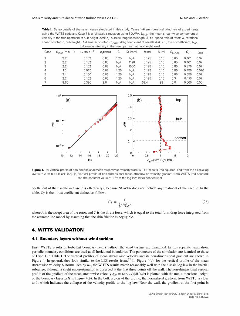
Figure 4. (a) Vertical profile of non-dimensional mean streamwise velocity from WiTTS’ results (red squared) and from the classic loglaw with � D 0.41 (black line). (b) Vertical profile of non-dimensional mean streamwise velocity gradient from WiTTS (red squared)

and the constant value of 1 from the log law (black dashed line).

coefficient of the nacelle in Case 7 is effectively 0 because SOWFA does not include any treatment of the nacelle. In thetable, CT is the thrust coefficient defined as follows

CT DT

12�U2

hubA(28)

where A is the swept area of the rotor, and T is the thrust force, which is equal to the total form drag force integrated fromthe actuator line model by assuming that the skin friction is negligible.

4. WITTS VALIDATION

4.1. Boundary layers without wind turbine

First, WiTTS results of turbulent boundary layers without the wind turbine are examined. In this separate simulation,periodic boundary conditions are used at all horizontal boundaries. The parameters of the simulation are identical to thoseof Case 1 in Table I. The vertical profiles of mean streamwise velocity and its non-dimensional gradient are shown inFigure 4. In general, they look similar to the LES results from.27 In Figure 4(a), for the vertical profile of the meanstreamwise velocity U normalized by u�, the WiTTS results match reasonably well with the classic log law in the inertialsubrange, although a slight underestimation is observed at the first three points off the wall. The non-dimensional verticalprofile of the gradient of the mean streamwise velocity �m D .�z=u�/.dU=dz/ is plotted with the non-dimensional heightof the boundary layer z=H in Figure 4(b). In the bulk region of the profile, the normalized gradient from WiTTS is closeto 1, which indicates the collapse of the velocity profile to the log law. Near the wall, the gradient at the first point is



underestimated, which causes an ‘overshoot problem’ at z=H < 0.1.42 However, note that the hub height of the windturbine is about z=H � 0.27, where �m � 0.955 and the bottom tip level of the rotor is at z=H � 0.11, where �m � 1.12.Therefore, we found that the simulation within the rotor region is minimally affected by the slight disagreement of thelaw-of-the-wall scaling near the wall.

In Figure 5, the normalized streamwise spectra of streamwise velocity at several heights z=H are plotted as a function ofk1z, where k1 is the streamwise wave number. It appears that normalized spectra at different heights collapse well. In theinertial subrange (k1z > 1), the �5/3 power law scaling of the spectra is captured well by WiTTS, and in the productionsubrange (k1z < 1), the spectra follow a slope of �1.25, 27

In Figure 6, the vertical profiles of spatial averaged Smagorinsky coefficient < Cs,� > and the scale-dependent coef-ficient < ˇ > are plotted. Although a slight increase is observed from the interior region to about z=H � 0.1, theSmagorinsky coefficient < Cs,� > in the bulk region away from the wall is almost constant near 0.12, which impliesthat the turbulence is nearly homogeneous and isotropic, considering that the SGS mixing length ` D< Cs,� > isalmost constant. Below z=H � 0.1, < Cs,� > decreases fast to the wall, which is consistent with the fact that ` decreases

-5/3

-1z/H=0.008

0.070

0.477

0.289

0.383

0.195

0.102

Figure 5. Normalized streamwise spectra of streamwise velocity versus k1z, where u� D 0.102 m s�1.

z/H

0 0.04 0.08 0.12 0.160

0.1

0.2

0.3

0.4

0.5

<β>

z/H

0.4 0.6 0.8 10

0.1

0.2

0.3

0.4

0.5

Figure 6. Vertical profiles of (a) the Smagorinsky coefficient < Cs,� > and (b) scale-dependent parameter < ˇ >.



with z in that region. Further, the scale-dependent parameter < ˇ > is less than 1, which is consistent with the idea thatCs,4� < Cs,2� < Cs,�.25 In the interior region, < ˇ > is closer to 1, indicating that the scale dependence is weaker in thatregion, whereas near the wall, < ˇ > decreases faster because the scale dependence is stronger since the length scales ofturbulence shrink fast near the wall.

4.2. Boundary layer with a wind turbine

The WiTTS results of Case 1 are compared with the wind tunnel measurements reported in.21 The vertical profiles ofthe time-averaged, resolved, streamwise component of velocity u are plotted at several downstream sections in Figure 7.Note that, from this point on, .�/ denotes a time average instead of the test filtering used in the earlier sections and e.�/ isneglected for simplicity. In general, the WiTTS results match well with the wind tunnel data, especially in the region abovethe hub, although an overestimation of wind speed below the hub is also observed. This overestimation has two possiblecontributors: one is from the ‘overshoot problem’, shown in Figure 4(b) and Figure 7 at x=D D �1 by the overestimationof mean wind shear �m, and the other is the absence of the tower in our simulation. However, the overestimation is mainlyin the region below the rotor near the wall and its magnitude is small compared with the deficit in the rotor region. Thevelocity deficit is confined generally within the region of the turbine rotor and its maximum occurs behind the nacelle sincethe nacelle has a relatively large drag coefficient compared with the blades. The velocity deficit region, i.e. wake region,expands slowly downstream while its magnitude decreases. The velocity almost recovers back to its upstream profile after20D downstream.

Figure 8 compares the resolved streamwise turbulence intensity Ix, which is defined as the root mean square (rms) ofthe resolved streamwise velocity fluctuation component u0 D u � u divided by Uhub, resulted from the WiTTS and theexperiment. The simulated vertical profiles of Ix agree well qualitatively with the wind tunnel data, especially for thelocation of the maximum and minimum values. Both WiTTS and the wind tunnel data show that in general, turbulenceintensity is increased in the wake by the wind turbine, and at each downstream section, the maximum occurs near the top-tipheight due to the high wind shear. The global maximum appears near �5-7D downstream. Unlike velocity, turbulenceintensity recovers much slower and it is still noticeable after 20D especially in the region above hub height. Note that nearthe ground, an overestimate appears because of the less accurate scaling of the law-of-the-wall discussed earlier. But still,

Figure 7. Comparison of profiles of time-averaged mean streamwise component of velocity at several downstream sections on thevertical central plane.



Figure 8. Comparison of profiles of turbulence intensity Ix at several downstream sections on the vertical central plane.

this numerical problem appears only in the region near the wall and does not seem to affect the rotor region, which is thefocus of this paper.

The vertical profiles of the kinematic shear stress �u0w0 including its SGS part are compared in Figure 9. In the rotorregion, the wake exhibits two opposite behaviors above and below the hub height. Above the hub height, the shear stress(equal and opposite in sign to the turbulent momentum flux) is positive and enhanced by the wind turbine, which impliesa stronger downward turbulent momentum flux with the wind turbine than without it. Two maxima are found: the first oneat the top-tip height, lasting almost throughout the entire wake and the second maximum near the hub height in the nearwake region < 2D. Below the hub height, shear stress is enhanced too but with a negative sign in the wake < 10D, whichimplies a stronger upward turbulent momentum flux with the turbine than without it. This suggests that entrainment occursin such a way that enhanced downward momentum flux is found above the hub height and enhanced upward momentumflux below the hub height.

In summary, although some discrepancies exist between the results of WiTTS and the experiments in the region nearthe wall, in most part of the boundary layer and in the wake region, they match well. Since we are interested in the rotorregion, which is away from the wall, WiTTS appears to be a valid choice for this study.

5. RESULTS

5.1. Mean velocity properties

The self-similarity of a wake after a bluff body has been studied for decades.35, 43 In a fully developed wake, thetime-averaged, resolved, streamwise velocity deficit ıU.x, y, z/ D uinflow.z/ � u.x, y, z/, normalized by its maximumıUmax.x/, can be expressed as one function as

ıU.x, y, z/

ıUmax.x/D f .�/ (29)

where f .�/ is a self-similar shape function of �.x, y, z/ D r.y, z/=r 12.x/, r is the distance from the centerline of the wake and

r 12.x/ is the half-width, which is defined as the spanwise distance between two points on a profile at which the mean deficit



Figure 9. Comparison of profiles of the kinematic shear stress �u0w0 at several downstream sections on the vertical central plane.

is half of its maximum. The assumption of self-similarity is critical in several wind turbine wake models.5, 6, 44 However,this assumption is still arguable considering that a rotating wind turbine is much more complicated than a still bluff body. Inorder to clarify it, the normalization is carried out upon the profiles of ıU for Cases 1, 4, 5 and 6 in the horizontal plane atthe hub height and in the vertical central plane, respectively. A theoretical Gaussian function obtained with the hypothesisof uniform eddy viscosity (,35 p. 154) in the following form is used for comparison

f .�/ D exp.��2 ln 2/ (30)

As shown in Figure 10, in the bulk region of the wake, the self-similarity assumption with the Gaussian shape worksreasonably well in the horizontal plane, especially for � 1. The deviation from the Gaussian shape increases with theradius toward the edge of the wake where the shear is strong. Also, in the near wakes, e.g. x=D 3, Case 6 shows a smallbut noticeable deviation from the Gaussian curve. This implies that the self-similarity in the near wake depends on thespecific design of the rotor and nacelle. An extreme example showing the effect of the nacelle design is plotted in Figure 11,where the non-dimensional mean streamwise velocity deficit ıu=Uhub of Cases 1 and 7 are compared. Recall that Case 1is a wind tunnel scale simulation by WiTTS with nacelle, whereas Case 7 is a full-scale simulation by SOWFA withoutnacelle. Clearly, the discrepancy is significant in the near wake region. In Case 1, a single maximum deficit is found alongthe centerline. In contrast, two deficit maxima are observed in Case 7, each centered approximately at half the rotor radius.After 6D downstream, the two maxima merge together gradually at the centerline with the expanding of the annular shearlayer. The two cases become similar only after about 7D, and the self-similarity for Case 7 appears much later than for Case1. Nevertheless, the specific design of a turbine only has a significant effect in the near or intermediate wake region, but inthe far wake region, e.g., x=D > 7, the wake is less influenced by the turbine design and shows self-similar properties well.

Similarly, vertical profiles of velocity deficit are shown in Figure 12. Basically, self-similarity holds well in the upperhalf of the profiles, although small deviations are also found near the wake edges. In the lower parts of the profiles, however,self-similarity is preserved up to � � �1. Below that, it is invalidated by the strong shear near the ground, especially forCase 5 in Figure 12(c), in which u� is the strongest among the four cases. In summary, the assumption of self-similarityis verified in the bulk region of the wake both horizontally and vertically, but it only holds in the far wake region since inthe near wake, the design of the nacelle has a significant impact. Also, the self similarity is less valid, where wind shear isstrong, e.g. near the edges of the wake or near the ground.



Figure 10. Self-similarity profiles of time-averaged resolved streamwise velocity deficit in the horizontal plane at the hub height for(a) Case 1; (b) Case 4; (c) Case 5; and (d) Case 6. The velocity deficits are normalized by its value at the centerline. The y-axis is the

radial coordinate r D d=2 normalized by the half-width r 12

at that section.

Figure 11. Contours of non-dimensional time-averaged resolved streamwise velocity deficit in the horizontal plane at hub height for(a) Case 1 and (b) Case 7. The deficit is normalized by Uhub.

To evaluate wake effects or develop wake models, it is important to study how the wake develops with distance. Sinceself-similarity is often assumed, the evaluation of ıUmax.x/ is critical, and different relationships are used in different wakemodels. As shown in Figures 10 and 12, the maximum always appears near the centerline of the wake in cases wherethe nacelle effect is not negligible. Therefore, ıUhub is often used, since it is easier to measure. By fitting data from fieldmeasurements, Barthelmie et al.45 proposed

ıUhub

U1D c1

� x

D

�c2(31)

where U1 is the mean wind speed upstream and c1 and c2 are constants with values of (1.03, �0.97) or (1.07, �1.11),which are equally plausible.



(a) (b)

(d)(c)

Figure 12. Self-similarity profiles of time-averaged streamwise velocity deficit in the vertical central plane for (a) Case 1; (b) Case 4;(c) Case 5; and (d) Case 6. The velocity deficits are normalized by its value at the centerline. The y-axis is the radial coordinate r D d=2

normalized by the half-width r 12

at that section.

The widely used Jensen’s model6, 9 assumes a top-hat function for f .�/ in Equation (29), such that ıUmax.x=D/ DıU.x=D/ is constant inside the wake at x=D that yields

ıU

U1D a0

�1

1C 2kwakexD

�2

(32)

based on a linear expansion of the wake. Here, a0 D 2a D .1�p

1 � CT / is twice of the induction factor a, CT is the thrustcoefficient, kwake D A= ln.hhub=z0/ is a wake decay constant, A � 0.521 and z0 is the surface roughness length. The wakediameter Dw.x/ at distance x is determined by

Dw.x/ D�

1C 2˛0x

D

�D (33)

where ˛0 is a constant rate of expansion of the wake radius.With similar assumptions of top-hat profiles and linear expansion of the wake, an analytical modeling was proposed by

Frandsen et al.5 using momentum conservation in the wake as follows:

ıU

U1D

1

2˙

1

2

s1 � 2

A0

A.x/CT (34)

Here, A0 is the incident rotor area and A.x/ is the area of the cross section of the wake at distance x. The ‘C’ applieswhen a0 > 0.5 and � applies when a0 0.5. In the absence of wind shear, the cross section of the wake is a circle, i.e.

A.x/ D ��

Dw2

�2and

Dw.x/ D�ˇk=2 C ˛

x

D

�1=kD (35)

Here, ˇ D 12

1Cp

1�CTp1�CT

, k D 3 and

˛ D ˇk=2��

1C 2˛0x

D

�k� 1

� x

D

�(36)



Recently, based on LES results, Bastankhah and Porté-Agel44 proposed a new analytical model from the conservationof mass and momentum. The self-similarity property is used with a uniform Gaussian distribution of the velocity deficitas follows:

ıUhub

U1D 1 �

s1 �

CT

8.k�x=DC "/2(37)

where k� D @�=@x is the growth rate of the wake, � is the standard deviation of the velocity deficit that will be discussedlater, " D 0.2

pˇ and ˇ D 0.5.1 C

p1 � CT /=

p1 � CT . By using the Gaussian distribution, the velocity deficit at any

position .x, y, z/ can be found as

ıu.x, y, z/

U1DıUhub.x/

U1exp

��

1

2.k�x=DC "/2

�� z � zh

D

�2C� y

D

�2�

(38)

where zh is the hub height.In Figure 13, we present the non-dimensional velocity deficit at hub height ıUhub=Uhub from our LES results together

with the wake model predictions described earlier. The LES results show that in the near wake region, the curve shapeshighly depend on the incoming wind conditions and nacelle designs. We find it interesting that Case 7, which has no nacelle,shows an increase of the deficit with distance from almost zero to its maximum at about 6D to 7D, which correspondsto the merge of the two maxima of deficit at the centerline shown in Figure 11(b). For those cases with higher drag ofthe nacelle, the maximum appears faster with larger magnitude. In the far wakes, all the cases decrease gradually, andthe rate of decay decreases with distance. In Figure 13(a), the Barthelmie’s empirical model with two sets of suggestedparameters is also plotted. Since this model is based on field measurements, it gives fair prediction to some of our LESdata in the far wakes when c1 D 1.03, c2 D �0.97 are used. However, the magnitudes are underestimated by both choices.Moreover, the curves of the deficits do not converge for different conditions such that it is hard to fit all curves by using onlyone or two relationships. The Jensen’s model and Frandsen’s model are used in Figure 13(b,c), respectively. Since bothmodels start from the top-hat assumption of the deficit distribution, they underestimate the velocity deficit at the centerlinesignificantly. The Bastankhah’s model plotted in Figure 13(d) appears to be the best of the three candidates. It successfullycaptures the non-converging curves due to different CT and matches reasonably well with each individual case. However,it still underestimates the magnitude and overestimates the rate of decrease of the deficit with distance in the far wake. The

(b)

(d)

(a)

(c)

Figure 13. Non-dimensional time-averaged streamwise velocity deficit at hub height with LES and with several wake models. Thevelocity deficits are normalized by upstream mean wind speed at hub height Uhub. The symbols are LES results and lines are wakemodel results. The Barthelmie’s model (Equation (31)) is used in (a) and c1 D 1.03, c2 D �0.97 are used for the black solid lineand c1 D 1.07, c2 D �1.11 are used for the red solid line; the Jensen’s model (Equation (32)) is used in (b); the Frandsen’s model

(Equation (34)) is used in (c); and the Bastankhah’s (Equation (37)) model is used in (d).



discrepancies are possibly caused by the assumption that the wake grows isotropically in all directions perpendicular to thewind direction, without consideration of the azimuthal variation caused by the ambient wind shear, as discussed next.

In order to quantify the wake growth, the standard deviation � (square root of the variance �2) of the mean velocitydeficit ıu.x/ at each cross section is often treated as a proxy for the width (or spread) of the wake. The variance is calculatedas follows:

�2 D1

M0

Z 1�1

.x � �/2ıu.x/dx D M2=M0 � �2 (39)

Here, � D M1=M0 is the mean and M0, M1 and M2 are the zeroth, first and second moments, respectively, defined as

M0 D

Z 1�1

ıu.x/dx, M1 D

Z 1�1

xıu.x/dx, M2 D

Z 1�1

x2ıu.x/dx (40)

For a Gaussian distribution, a spread of 4� includes approximately 95% of the area under the distribution, thus, it is oftenused as the ‘boundary’ of the wake. Accordingly, the non-dimensional standard deviation normalized by the rotor diametercan be calculated horizontally at the hub height level and vertically in the vertical central plane, respectively (Figure 14).The prediction from the Jensen’s model Equation (33) is also shown as a comparison, in which ˛0 D 0.05 is chosen. For thehorizontal expansion of the wake at the hub height level, the linear assumption used in the Jensen’s model actually workswell. The LES results approximately follow the same rate of linear expansion, although they grow a bit faster in the region5 < x=D < 10 and a slightly slower past 10D [Figure 14(a)]. On the other hand, for the vertical expansion of the wake[Figure 14(b)], the LES results depart significantly from the Jensen’s wake model. The expansions are slower in overalland the discrepancies increase with distance, which imply an anisotropy in the wake growth. Another linear relationship1C 0.07x=D was used in Figure 14(b) to better fit the curves, i.e. ˛0 D 0.035. Note that this fitting is not perfect since theLES curves appear less linear in the far wakes, but it is used here only for its simplicity.

To examine this anisotropy, contours of non-dimensional velocity deficit ıu=ıumax, where ıumax is the maximum ofthe deficit at the cross section, are plotted at several vertical cross sections downstream in Figure 15 for Case 1. Theboundary of the wake is represented by the contour line of ıu=ıumax D 0.136, corresponding to the value at 4� of a normaldistribution. As shown in Figure 15(a,b), the anisotropy is relatively small all the way to about x=D � 8, as the contours arequalitatively symmetric and circular, which suggests that the wake models produce reasonably good predictions. However,the wake expansion is still slightly slower vertically than horizontally because of vertical wind shear, as shown by the moreelliptic than circular shape. But the difference between the axes are small so the shape does not change too much. In thefurther downstream wake regions [Figure 15(c,d)], besides the vertical wind shear, the anisotropy is primarily caused bythe impact of the wake with the ground, which causes the wake to spread out laterally near the ground and the elliptic shapeto be destroyed. However, this effect is limited in the lower part and the rest of the wake is less affected.

Looking back at the Bastankhah’s model, it is clear that ignoring the anisotropic wake expansion causes an overestimateof the area of wake in the far wake region, especially when the wake hits the ground. Therefore, the mean velocity deficit isunderestimated because of conservation of mass and momentum, whereas the decay rate is overestimated. Here, a simple

(b)(a)

Figure 14. The wake width represented by 4�=D along the streamwise direction, where D is the rotor diameter and � is the standarddeviation of mean velocity deficit: (a) in the horizontal plane at the hub height level, representative of horizontal wake expansion and

(b) in the vertical central plane, representative of vertical wake expansion.



(a) (b)

(c) (d)

Figure 15. Contours of non-dimensional mean velocity deficit of Case 1 on the cross sections at (a) x=D D 2, (b) x=D D 8.0, (c)x=D D 14.0 and (d) x=d D 18.0. The velocity deficit is normalized by the maximum of deficit ıUmax at each section. The black solidline represents the contour line of ıu=ıumax D 0.136. The white and red dashed lines are the predicted wake boundary from the

Jensen’s model and the Frandsen’s model, respectively.

modification is proposed to take the anisotropic wake expansion into account. Instead of using the same � in all directions,an elliptical Gaussian function corresponding to �y ¤ �z can be used in the following relationship

ıu.x, y, z/

U1DıUhub.x/

U1exp

�

y2

2�2yC.z � zh/

2

2�2z

!!(41)

As shown in Figure 14, we can simply use the linear estimations of �y and �z as

�y

DD ky

x

DC ",

�z

DD kz

x

DC " (42)

where ky and kz are the expansion rates of the wake in the horizontal and vertical directions, respectively, and " is definedin Equation (37). As a consequence of Equation (41), by equating the momentum loss to the total thrust force followingthe same procedure of Bastankhah and Porté-Agel,44 Equation (37) can be rewritten as

ıUhub

U1D 1 �

s1 �

CT

8�y�z

D2

(43)

Note that Equation (43) coincides with Equation (37) when �y D �z.The modified model Equation (43) is tested by using the present cases and ky D 0.025, kz D 0.0175 from the observation

of Figure 14. Note that the expansion rates are not constant but vary case by case, as shown in44 and.46 Comparisonsbetween the modified model and the original model are shown in Figure 16. As discussed earlier, the Bastankhah’s originalmodel underestimates the values of velocity deficit in the far wakes in Figure 16(a), meanwhile, the modified model reducesthis underestimation noticeably and matches better with the LES results in Figure 16(b). It shows that the anisotropy in thewake expansion is important to get the correct estimation of the velocity deficit. Note that the linear fit of the expansion rateis only the first-order approximation. Higher-order fittings are possible and can be embedded easily into the current model.

5.2. Turbulence properties

The turbulence intensity in the wake of a wind turbine is important to the performance and wind load of the wind turbinessitting behind. In Figure 17, contours of the three components of the resolved turbulence intensity of Case 1 are plotted in



(b)(a)

Figure 16. Comparisons of the modified Bastankhah’s model and Bastankhah’s original model for non-dimensional time-averagedstreamwise velocity deficit at hub height. The symbols are LES results and the dashed lines in (a) are from the original Bastankhah’

model and in (b) are from the modified model.

(b)

(c)

(a)

Figure 17. Turbulence intensity of Case 1: (a) streamwise component Ix , (b) spanwise component Iy and (c) vertical component Iz .

the vertical central plane. In the near wake region, the nacelle induces a significant increase of Ix that lasts only about 2Ddownstream. An increase in Ix also happens at the top-tip level of the rotor, which continuously increases and reaches itsmaximum at about 5D downstream in this case and lasts until about 15D. Therefore, this effect of Ix is very important todownstream wind turbines in a modern wind farm with a typical spacing of about 8D � 10D. An interesting finding is thata low turbulence intensity region forms past the wind turbine beneath the rotor level in the wake. This decreased turbulenceintensity is caused by the net effect of the reduced wind shear induced by the turbine and the background wind shear.4

Compared with the streamwise component, the other components Iy and Iz are less significant, as expected[Figure 17(b,c)]. The spanwise intensity Iy also shows an asymmetry due to wind shear that is larger above hub height thanbelow. At the hub height level, Iy slightly increases not directly past the nacelle but at a distance of about 0.5D downstream.The maximum of Iy occurs roughly at the same distance as Ix, at about 6 � 7D, but at a vertical location that is lower than



the top-tip level. The flow separation at the edge of the nacelle induces a significant increase of Iz in the near wake, whereasa small increase of Iz is observed at the tips of the rotor. Because of its dominance, Ix is of particular interest and will besimply referred as the turbulence intensity I in this study, as done in many other works.3

In order to show the wind turbine effect on turbulence intensity, the added turbulence intensity can be defined as4

4I Dq

I2wake � I2

1 (44)

where I1 is the turbulence intensity in the free upstream. Although an exact description of the 3D distribution of theturbulence intensity is complex, in practice, it is useful to model the maximum added turbulence intensity in a relativelysimple way. As discussed earlier, the maximum always appears near the top-tip level of the annular shear layer of thewake. In the near wake region, by assuming that the production of TKE is much larger than its dissipation, Crespo andHernández4 proposed a theoretical expression for the maximum added turbulence intensity4Im

4Im D 0.75a D 0.362Œ1 � .1 � CT /1=2� (45)

where a is the induction factor and CT is the thrust coefficient. In Figure 18, 4Im at the top-tip level within x < 3D fromthe LES cases are plotted with the theoretical model. In general, the WiTTS results show very good agreements with thetheoretical model in the range 0.3 < CT < 0.6, where4Im increases mainly with CT in the near wake region.

For the far wakes, by fitting the UPMWAKE results in the region 5 < x=D < 15 with 0.07 < I1 < 0.14, Crespo andHernández4 proposed that the maximum added turbulence intensity is related to the induction factor a and free upstreamturbulence intensity I1 as follows

4Im D 0.73a0.8325I�0.03251

� x

D

��0.32(46)

Alternatively, Quarton47 proposed an empirical relationship

4Im D 4.8C0.7T I0.681

�x

xN

��0.57

(47)

where xN is the estimated length of the near wake using the definition by Vermeulen8 as

xN D

p0.214C 0.144 m.1 �

p0.134C 0.124 m/

.1 �p

0.214C 0.144 m/p

0.134C 0.124 m

r0

dr=dx(48)

where m D 1p1�CT

, r0 D Rq

MC12 and R is the radius of the rotor. In Equation (48), dr=dx is the expansion rate of the wake

that has three contributors: ambient turbulence, .dr=dx/2a D 2.5I0C0.005; rotor generated turbulence, .dr=dx/2r D 0.012B�;

X

0.2 0.4 0.6 0.8

0.1

0.2

0.3Case 1Case 2Case 3Case 4Case 5Case 6Case 7Crespo & Hernandez (1996)

X

Figure 18. The maximum added turbulence intensity 4Im of the LES cases versus the theoretical model from Crespo andHernández (1996).



and shear generated turbulence, .dr=dx/2m D.1�m/

p1.49Cm

9.76.1Cm/ , where B is the number of blades and � is the rotor-tip speed

ratio. A modification form of the Quarton’s model based on the wind tunnel measurements was proposed by Hassan48 as

4Im D 5.7C0.7T I0.681

�x

xN

��0.96

(49)

Those three models are actually quite similar to each other in form considering that a and CT are strongly linked. Thebiggest discrepancy is that4Im slightly decreases with I1 in Equation (46), whereas it increases with I1 in Equations (47)and (49). The three models are tested for all cases in this paper and the results are compared with the LES data. The resultsare shown in Figure 19, where only Case 2 is omitted since it is very close to Case 1. The LES results show that, althoughthe incoming turbulence intensity is the same for Cases 1 to 6, the added turbulence intensities are still scattered caused bythe differences in wind speed, rotation speed of rotor or nacelle design. But all cases share a very similar pattern, i.e., the4Im increases quickly in the near wake region until it reaches a maximum, then it gradually decreases. The point where4Im is maximum varies depending on the specific case, but in general, it is in the range between about 4D and 8D. Itis clear that neither of the three wake models match well with the LES results in the near or intermediate wake regions.The Quarton’s model overestimates the added intensity significantly, whereas the Crespo’s model underestimates both themagnitude of the added intensity and its rate of decaying with distance. The Hassan’s model appears to have better matchto the LES results, but still, it underestimates the magnitude in the far wake regions.

Based on the observations, a modification to the Hassan’s model is proposed here as follows

4Im D 5.7C0.5T I0.681

�x

xN

��0.96

(50)

Note that the only explicit change made here is the power of CT . Since xN is also a function of CT , the change also affectsthe estimation of xN for each case. As shown in Figure 19(d), although the magnitude of 4Im is still underestimated inthe far wake at distances greater than 16D and the rate of change is slightly overestimated, the current model improvesthe prediction and fits the curves of LES results better compared with the other three models. The modification is purelyempirical and simple, thus, a more comprehensive investigation is expected in future studies.

It is also interesting to study the budget of TKE in the wind turbine wakes. In Figure 20, the following four terms of theTKE budget, averaged over Cases 1–5, are plotted in the vertical central plane: advection of TKE by mean flow

� uj@k

@xj(51)

(b)(a)

(d)(c)

Figure 19. The added turbulence intensity at the top-tip level of rotor with comparisons of several wake models. The symbols are LESresults and dashed lines are wake model results. The Quarton’s model (Equation (47)) is used in (a), the Crespo’s model (Equation (46))

is used in (b), the Hassan’s model (Equation (49)) is used in (c) and our new model (Equation (50)) is used in (d).



z/D

0 3 6 9

0.5

1

1.5

2 30

-30

TA

z/D

0 3 6 9

0.5

1

1.5

2 10

-10

TTz/

D

0 3 6 9

0.5

1

1.5

2 30

0

TP

x/D

z/D

0 3 6 9

0.5

1

1.5

2 0

-10

TD

Figure 20. The budget of turbulent kinetic energy averaged over all WiTTS cases. TA: TKE advection by mean flow; TT: TKE transportby eddies; TP: TKE production; TD: TKE dissipation. All terms are normalized by the corresponding u3

�=D.

transport of TKE by the eddies

�@ku0i@xi

(52)

TKE production by shear

u0iu0j@ui

@xj(53)

and dissipation

� 2�rS0ijS0ij (54)

where .�/ denotes the time average, k D 12

��u01�2C�u02�2C�u03�2� is TKE, u0i is the velocity fluctuations and S0ij is the

rate of strain tensor of the velocity fluctuations as follows

S0ij D1

2

@u0i@xjC@u0j@xi

!(55)

and �r is an eddy viscosity from Equation (5). All terms are normalized by its corresponding u3�=D of each case.

In general, the TKE advection by the mean flow and the TKE transport by the eddies behave in a very similar manner: alarge positive value after the nacelle occurs but is limited within 3D; opposite signs on either sides of the rotor are observedwithin 1D upwind and downwind; and a relatively strong negative value is generated at near the top-tip level that lastsabout 5D downstream due to the presence of the TKE maximum at about 5D. Moreover, the magnitude of the advectionby mean flow is larger than the transport by eddies in the near wake region. Because of the asymmetry of the vertical windshear, the advection and transport are both weak at the lower levels beneath the rotor.

The TKE production caused by wind shear at the top-tip level of the rotor is significant. The nacelle forms two regions ofenhanced TKE production, above and below its edges. The high production region above the nacelle merges with the high



production region at the top-tip level at about 3D. The TKE dissipation mainly happens in the near wake region past thenacelle and is weak in the rotor region, consistent with the assumption used to derive Equation (45). In the far wake, a localmaximum of dissipation happens in the upper part above the hub level but below the top-tip level, whereas the dissipationnear the ground appears to be unaffected by the turbine.

6. CONCLUSIONS

In this study, a new LES code, the WiTTS, is developed to study the wake generated from a single wind turbine in the neutralABL. A scale-dependent Lagrangian dynamic model is used for the SGS stress, and the actuator line model is used to takeinto account the rotational effect of the rotor. The WiTTS results match well with wind tunnel measurements, although thescaling of the law-of-the-wall shows a classic ‘overshoot’ problem near the ground. The mean velocity deficit shows goodself-similarity properties following a normal distribution in the horizontal plane at the hub height level. Self-similarity isa less valid approximation in the vertical near the ground due to strong wind shear. The wake expansion is found to beanisotropic due to the wind shear and impact with the ground, such that the wake grows faster horizontally than vertically.Several wake models of the velocity deficits are examined and compared against our LES results. A modification to theBastankhah’s model is proposed to take into account the anisotropic expansion of the wake in a simple way by assumingtwo different variances in the vertical and in the horizontal directions rather than the same one in both directions. Theresults show that the modification improves the prediction in the far wake regions.

Aligned with the mean wind direction, the streamwise component of turbulence intensity is the dominant one among thethree components, and thus, it is further studied here. The highest turbulence intensity occurs near the top-tip level. TheWiTTS results prove that the theoretical model proposed by Crespo and Hernández works well to predict the maximumadded turbulence intensity 4Im in the near wake region. In the far wake, the LES results are used to test several wakemodels for the added turbulence intensity. An empirical modification is also proposed to the Hassan’s model for betterfitting in the far wakes. The budget of turbulence kinetic energy from the WiTTS are is also evaluated. It is found that theadvection of TKE by the mean flow is important in the near wake, and the transport of TKE by eddies has a similar patternbut lower magnitude. The TKE production is affected significantly by the nacelle in the near wake and at the top-tip level ofthe rotor, lasting several rotor diameters downstream. The TKE dissipation is relatively small in the whole wake, althoughit is significantly increased by the nacelle wake within 2D.

In future work, we plan to improve WiTTS to better predict the law-of-the-wall near the ground. Brasseur and Wei42

studied this in detail and showed that the issue can be remedied by changing the grid cell aspect ratio. Previous studieshave already shown that atmospheric stability can have a significant influence on the wake properties15, 49, 50 and viceversa. Therefore, the stable and unstable atmospheric conditions, not only neutral, will also be studied by using improvednumerical tools. Lastly, WiTTS will be expanded to treat multiple, overlapping wakes from several wind turbines.

REFERENCES

1. Global Wind Statistics. Global wind energy council, 02/11/2013, 2012.2. Crespo A, Hernández J, Frandsen S. Survey of modelling methods for wind turbine wakes and wind farms. Wind

Energy 1999; 2: 1–24.3. Vermeer LJ, Crespo A. Wind turbine wake aerodynamics. Progress in Aerospace Sciences 2003; 39: 467–510.4. Crespo A, Hernández J. Turbulence characteristics in wind-turbine wakes. Journal of Wind Engineering and Industrial

Aerodynamics 1996; 61: 71–85.5. Frandsen S, Barthelmie R, Pryor S, Rathmann O, Larsen S, Høstrup J, Thøgersen M. Analytical modelling of wind

speed deficit in large offshore wind farms. Wind Energy 2006; 9: 39–53.6. Jensen NO. A note on wind turbine interaction. Risø-M-2411, Risø National Laboratory, Roskilde, 1983.7. Lissaman PBS. Energy effectiveness of arbitrary arrays of wind turbines. Journal of Energy 1979; 3: 323–328.8. Vermeulen PEJ. An experimental analysis of wind turbine wakes. Proceedings of the 3rd International Symposium on

Wind Energy System, Lyngby, Denmark, August 26–29, 1980; 431–450.9. Katic I. A simple model for cluster efficiency. Proceedings of the European Wind Energy Association Conference and

Exhibition, Rome, Italy, 1986; 407–409.10. Troldborg N. Actuator line modeling of wind turbine wakes. PhD Thesis, Technical University of Denmark, 2008.11. Sforza PM, Sheering P, Smorto M. Three-dimensional wakes of simulated wind turbines. AIAA Journal 1981; 19:

1101–1107.12. Ainslie JF. Calculating the field in the wake of wind turbines. Journal of Wind Engineering and Industrial

Aerodynamics 1988; 27: 213–224.



13. Ivanell S, Sørensen JN, Mikkelsen R, Henningson D. Analysis of numerically generated wake structures. Wind Energy

2009; 12: 63–80.

14. Jimenez A, Crespo A, Migoya E, Garcia J. Advances in large-eddy simulation of a wind turbine wake. Journal of

Physics: Conference Series 2007; 75: 012041.

15. Lu H, Porté-Agel F. Large-eddy simulation of a very large wind farm in a stable atmospheric boundary layer. Physics

of Fluids 2011; 23: 065101.

16. Sørensen JN, Shen WZ, Mundate X. Analysis of wake states by a full-field actuator disc model. Wind Energy 1998; 1:

73–88.

17. Sørensen JN, Shen WZ. Numerical modeling of wind turbine wakes. Journal of Fluids Engineering 2002; 124:

393–399.

18. Wu YT, Porté-Agel F. Large-eddy simulation of wind-turbine wakes: evaluation of turbine parametrisations.

Boundary-Layer Meteorology 2011; 138: 345–366.

19. Calaf M, Meneveau C, Meyers J. Large eddy simulation study of fully developed wind-turbine array boundary layers.

Physics of Fluids 2010; 22: 015110.

20. Calaf M, Parlange MB, Meneveau C. Large eddy simulation study of scalar transport in fully developed wind-turbine

array boundary layers. Physics of Fluids 2011; 23: 126603.

21. Chamorro LP, Porté-Agel F. Effects of thermal stability and incoming boundary-layer flow characteristics on

wind-turbine wakes: a wind-tunnel study. Boundary-Layer Meteorology 2010; 136: 515–533.

22. Troldborg N, Sørensen JN, Mikkelsen R. Actuator line simulation of wake of wind turbine operating in turbulent

inflow. The Science of Making Torque from Wind, Journal of Physics: Conference Series 2007; 75: 012063.

23. Crespo A, Manuel F, Moreno D, Fraga E, Hernández J. Numerical analysis of wind turbine wakes. In Proceedings of

Delphi Workshop on Wind Energy Applications, Delphi, Greece, 1985; 15-25.

24. Moeng C. A large-eddy simulationmodel for the study of planetary boundary-layer turbulence. Journal of the

Atmospheric Sciences 1984; 46: 2052–2062.

25. Porté-Agel F, Meneveau C, Parlange MB. A scale-dependent dynamic model for large-eddy simulation: application to

a neutral atmospheric boundary layer. Journal of Fluid Mechanics 2000; 415: 261–284.

26. Germano M, Piomelli U, Cabot WH. A dynamic subgrid-scale eddy viscosity model. Physics of Fluids A 1991; 3:

1760–1765.

27. Bou-Zeid E, Parlange MB, Meneveau C. A scale-dependent Lagrangian dynamic model for large eddy simulation of

complex turbulent flows. Physics of Fluids 2005; 17: 025105.

28. Meneveau C, Lund T, Cabot W. A Lagrangian dynamic subgrid-scale model of turbulence. Journal of Fluid Mechanics

1996; 319: 353–385.

29. Harlow FH, Welch JE. Numerical calculation of time-dependent viscous incompressible flow of fluid with free surface.

Physics of Fluids 1965; 8: 2182–2189.

30. Liu X, Osher S, Chan T. Weighted essentially non-oscillatory schemes. Journal of Computational Physics 1994; 115:

200–212.

31. Vasilyev OV. High order finite difference schemes on non-uniform meshes with good conservation properties. Journal

of Computational Physics 2000; 157: 746–761.

32. Kim J, Moin P. Application of a fractional-step method to incompressible Navier-Stokes equations. Journal of

Computational Physics 1985; 59: 308–323.

33. McAdams A, Sifakis E, Teran J. A parallel multigrid Poisson solver for fluids simulation on large grids. Proceedings

of Eurographics/ ACM SIGGRAPH Symposium on Computer Animation, Madrid 2-4th July, 2010; 65–74.

34. Smagorinsky J. General circulation experiments with the primitive equations: I. The basic experiment. Monthly

Weather Review 1963; 91(3): 99–164.

35. Pope SB. Turbulent Flows. Cambridge University Press: New York, 2000.

36. Lilly DK. A proposed modification of the Germano subgrid-scale closure method. Physics of Fluids A 1992; 4:

633–635.

37. Manwell J, McGowan J, Rogers A. Wind Energy Explained: Theory, Design and Application. Wiley: New York, 2002.

577 pp.

38. Mikkelsen R. Actuator disc methods applied to wind turbines. PhD Dissertation, Technical University of Denmark,

2003.



39. Martinez LA, Leonardi S, Churchfield MJ, Moriarty PJ. A comparison of actuator disk and actuator line wind turbinemodels and best practices for their use. 50th AIAA Aerospace Sciences Meeting including the New Horizons Forumand Aerospace Exposition, Nashville, Tennessee, 09–12 January 2012.

40. Churchfield MJ, Lee S, Moriarty PJ, Martínez LA, Leonardi S, Vijayakumar G, Brasseur JG. A large-eddy simu-lation of wind-plant aerodynamics. 50th AIAA Aerospace Sciences Meeting including the New Horizons Forum andAerospace Exposition, Nashville, Tennessee, 09–12 January 2012.

41. Churchfield MJ, Lee S, Michalakes J, Moriarty PJ. A numerical study of the effects of atmospheric and wake turbulenceon wind turbine dynamics. Journal of Turbulence 2012; 13: 1–32.

42. Brasseur JG, Wei T. Designing large-eddy simulation of the turbulent boundary layer to capture law-of-the-wallscaling. Physics of Fluids 2010; 22: 021303.

43. Tennekes H, Lumley JL. A First Course in Turbulence. The MIT Press: Cambridge, MA, 1972.44. Barthelmie R, Larsen G, Pryor S, Jørgensen H, Bergström H, Schlez W, Rados K, Lange B, Vølund P, Neckelmann

S, Mogensen S, Schepers G, Hegberg T, Folkerts L, Magnusson M. ENDOW (efficient development of offshore windfarms): modelling wake and boundary layer interactions. Wind Energy 2004; 7: 225–245.

45. Bastankhah M, Porté-Agel F. A new analytical model for wind-turbine wakes. Renewable Energy 2014; 70: 116–123.46. Wu YT, Porté-Agel F. Atmospheric turbulence effects on wind-turbine wakes: an LES study. Energies 2012; 5:

5340–5362.47. Quarton DC. Wake turbulence characterization. Final report from Garrad Hassan and partners to the energy

technology support unit of the Department of Energy of the UK; Contract No. ETSUWN 5096, 1989.48. Hassan U. A wind tunnel investigation of the wake structure within small wind turbine farms. E/5A/CON/5113/1890.

UK Department of Energy, ETSU, 1992.49. Abkar M, Porté-Agel F. The effect of free-atmosphere stratification on boundary-layer flow and power output from

very large wind farms. Energies 2013; 6: 2338–2361.50. Roy SB, Traiteur JJ. Impacts of wind farms on surface air temperatures. Proceedings of the National Academy of

Sciences 2010; 107(42): 17899–17904.


Documents

Self-similarity and turbulence characteristics of wind turbine … Library/Our People/Profiles... · Self-similarity and turbulence characteristics of wind ... directly solving the