Self-Diagnosis for Detecting System Failures in Large-Scale Wireless Sensor Networks

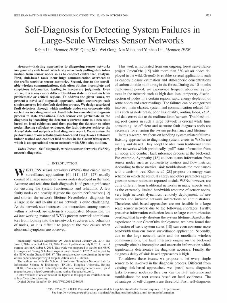
IEEE TRANSACTIONS ON WIRELESS COMMUNICATIONS, VOL. 13, NO. 10, OCTOBER 2014 5535

Self-Diagnosis for Detecting System Failures inLarge-Scale Wireless Sensor Networks

Kebin Liu, Member, IEEE, Qiang Ma, Wei Gong, Xin Miao, and Yunhao Liu, Member, IEEE

Abstract—Existing approaches to diagnosing sensor networksare generally sink based, which rely on actively pulling state infor-mation from sensor nodes so as to conduct centralized analysis.First, sink-based tools incur huge communication overhead tothe traffic-sensitive sensor networks. Second, due to the unreli-able wireless communications, sink often obtains incomplete andsuspicious information, leading to inaccurate judgments. Evenworse, it is always more difficult to obtain state information fromproblematic or critical regions. To address the given issues, wepresent a novel self-diagnosis approach, which encourages eachsingle sensor to join the fault decision process. We design a series offault detectors through which multiple nodes can cooperate witheach other in a diagnosis task. Fault detectors encode the diagnosisprocess to state transitions. Each sensor can participate in thediagnosis by transiting the detector’s current state to a new statebased on local evidences and then passing the detector to othernodes. Having sufficient evidences, the fault detector achieves theAccept state and outputs a final diagnosis report. We examine theperformance of our self-diagnosis tool called TinyD2 on a 100-nodeindoor testbed and conduct field studies in the GreenOrbs system,which is an operational sensor network with 330 nodes outdoor.

Index Terms—Self-diagnosis, wireless sensor networks (WSNs),network diagnosis.

I. INTRODUCTION

W IRELESS sensor networks (WSNs) that enable manysurveillance applications [6], [11], [25], [27] usually

consist of a large number of sensor nodes deployed in the wild.Accurate and real-time fault diagnosis is of great significancefor ensuring the system functionality and reliability. A fewfaulty nodes can heavily degrade the system performance [12]and shorten the network lifetime. Nevertheless, diagnosis fora large scale and in-situ sensor network is quite challenging.As the network size increases, the interactions among sensorswithin a network are extremely complicated. Meanwhile, thead hoc working manner of WSNs prevent network administra-tors from looking into the in-network structures and behaviorsof nodes, so it is difficult to pinpoint the root causes whenabnormal symptoms are observed.

Manuscript received September 29, 2013; revised January 21, 2014 andJune 6, 2014; accepted June 19, 2014. Date of publication July 8, 2014; date ofcurrent version October 8, 2014. This work was supported in part by the NSFCDistinguished Young Scholars Program under Grant 61125202 and in part bythe NSFC under Grant 61103187. The associate editor coordinating the reviewof this paper and approving it for publication was L. Libman.

The authors are with the School of Software, Tsinghua National Lab forInformatics Science & Technology (TNList), Tsinghua University, Beijing100084, China (e-mail: [email protected]; [email protected]; [email protected]; [email protected]; [email protected]).

Color versions of one or more of the figures in this paper are available onlineat http://ieeexplore.ieee.org.

Digital Object Identifier 10.1109/TWC.2014.2336653

This work is motivated from our ongoing forest surveillanceproject GreenOrbs [15] with more than 330 sensor nodes de-ployed in the wild. GreenOrbs enables several applications suchas canopy closure estimation and atmospheric concentrationsof carbon dioxide monitoring in the forest. During the 10 monthsdeployment period, we experience frequent abnormal symp-toms in the network such as high data loss, temporary discon-nection of nodes in a certain region, rapid energy depletion ofsome nodes and error readings. The failures can be categorizedinto two main classes, system and communication related fail-ures such as node crash, poor link quality, routing loops, et al.,and data errors due to the malfunction of sensors. Troubleshoot-ing root causes in such a large network is crucial while timeconsuming, so efficient and accurate fault diagnosis tools arenecessary for ensuring the system performance and lifetime.

In this research, we focus on handling system related failures.Existing approaches to diagnosing system errors in WSNs aremainly sink-based. They adopt the idea from traditional enter-prise networks which periodically “pull” state information fromall nodes and conduct fault inference process at the back-end.For example, Sympathy [18] collects status information fromsensor nodes such as connectivity metrics and flow metrics.According to these metrics, sink troubleshoots the root causeswith a decision tree. Zhao et al. [28] propose the energy scanscheme in which the residual energy and other parameter aggre-gates on sensor nodes are reported to sink. WSNs, however, arequite different from traditional networks in many aspects suchas the extremely limited bandwidth resource of sensor nodes,very high network dynamics, remotely deployment, ad hocmanner and invisible network interactions to administrators.Therefore, sink-based approaches are not feasible in a largescale sensor network due to the following shortages. Firstly,proactive information collection leads to large communicationoverhead that heavily shortens the system lifetime. Based on theexperience in our GreenOrbs deployment, we have found thatcollection of basic system states [18] can even consume morebandwidth than our forest surveillance application. Secondly,due to the large network scale and the unreliable wirelesscommunications, the fault inference engine on the back-endgenerally obtains incomplete and uncertain information whichsignificantly deteriorates the diagnosis accuracy. Finally, thediagnosis delay of sink-based approaches is high.

To address these issues, we propose to let every singlesensor to be involved in the diagnosis process. Different fromexisting sink-based approaches, we “push” some diagnosistasks to sensor nodes so they can join the fault inference andtroubleshoot the root causes based on local evidences. Theadvantages of self-diagnosis are threefold. First, self-diagnosis

1536-1276 © 2014 IEEE. Personal use is permitted, but republication/redistribution requires IEEE permission.See http://www.ieee.org/publications_standards/publications/rights/index.html for more information.

5536 IEEE TRANSACTIONS ON WIRELESS COMMUNICATIONS, VOL. 13, NO. 10, OCTOBER 2014

can save a large amount of transmissions by applying localdecision. Second, self-diagnosis avoids information loss on theway to sink and thus improves the accuracy. Finally, it providesrealtime diagnosis results.

In spite of all these benefits, employing a self-diagnosisstrategy in a large scale WSN is challenging. First, it is wellknown that the computation and storage resources at eachsensor are limited, so the components injected to nodes have tobe light-weight. Second, a sensor only has very narrow scopeon the system state and in many cases it can hardly determinethe root causes simply based on local evidences. Hence howto make multiple sensors cooperate with each other to detectnetwork failures needs to be addressed.

In this study, we present our new self-diagnosis tool calledTinyD2. We introduce our fault detectors based on the FiniteState Machines (FSMs). The fault detectors encode the diagno-sis process to state transitions. Each fault detector has severalstates, each of which indicates an intermediate step of the faultdiagnosis process. Taking the local information from each nodeas input, the fault detector switches its state. Thus, a sensor canparticipate in the diagnosis by transiting the state of the faultdetector to a new one based on local evidences and then deliverthe detector to other nodes. Fault detectors travel among sensornodes and continuously collect new evidences. When a detectorachieves its Accept state, the fault is pinpointed and a diagnosisreport can be formed accordingly. During the fault inferenceprocess, sensor nodes cooperate with each other to achieve thefinal diagnosis report that can assist network administratorsin conducting further diagnosis or failure recovery actions.The detectors are light-weight in terms of storage space andcomputation overhead. During the diagnosis process, messagesexchanged among sensors include not full detectors but only thecurrent state of them which is necessarily small in size. We alsoform the diagnosis trigger as a change-point detection problemand present a triggering strategy based on the cumulative sumcharts and a bootstrap scheme.

The major contributions of this work are as follows:

1) We study the problem of fault diagnosis in an operationalsensor network and present a novel self-diagnosis frame-work for large scale WSNs.

2) We design new fault detectors based on Finite StateMachines, through which multiple nodes cooperate witheach other and achieve diagnosis results.

3) We form the diagnosis triggering as a change-point de-tection problem and address it based on cumulative sumcharts and a bootstrap scheme.

4) We implement our self-diagnosis approach TinyD2 andconduct intensive experiments to examine its effective-ness in a 100 nodes testbed and a 330 nodes workingsystem.

The rest of this paper is organized as follows. Section II in-troduces existing efforts that are related to this work. Section IIIdescribes the fault detectors and the self-diagnosis process. Wediscuss the implementation details of TinyD2 in Section IV, andpresent the experimental results in Section V. We conclude thework in Section VI.

II. RELATED WORK

Both debugging and diagnosing approaches are related to thiswork. Debugging tools [12], [19] aim at finding software bugsand even agnostic failures in sensor networks. Clairvoyant [26]enables the source-level debugging for WSNs which allowspeople remotely execute standard debugging commands suchas step and break. Dustminer [9] focuses on troubleshootingunknown interactive bugs by mining the logs from sensornodes. Dustminer aims to find event sequences that are rareto see when the system works well and frequently appearwhen system performance degrees. Then the administratorslook into these suspicious sequences and locate the underlyingroot causes. Debugging tools are powerful at finding networkfaults, however, in cost of incurring huge control overhead,so they are generally used in the pre-deployment scenarios.Besides, debugging tools usually require human involvement.Instead, TinyD2 does not focus on exploring agnostic failuresin pre-deployed systems but aims to provide lightweight andefficient diagnosis services for operational WSNs.

However, a post-deployment WSN may experience manyfailures even when there is no bug in its software system. Thefocus of this research is troubleshooting performance failures innetworking and many existing efforts are related to our work.Some researchers propose to periodically scan parameters likeresidual energy [28] on sensor nodes. MintRoute [23] visual-ize the network topology by collecting neighbor tables fromsensor nodes and thus help to find link and route failures.SNMS [20] constructs network infrastructure for logging andretrieving state information at runtime and EmStar [2] sup-ports simulation, emulation and visualization of operationalsensor networks. Other researchers employ varying inferencestrategies for troubleshooting network faults. Sympathy [18]actively collects metrics such as data flow and neighbor tablefrom sensor nodes and determines the root causes based ona tree-like fault decision scheme. It can find faults on bothnode side and sink side. PAD [13] proposes the concept ofpassive diagnosis which leverages a packet marking strategy toderive network state and deduces the faults with a probabilisticinference model. PAD is designed to detect node and link levelerrors. Megan et al. [21] present Visibility, a new protocoldesign that aims at reducing the diagnosis overhead. PD2 [1]is a data-centric approach that tries to pinpoint the root causesof application performance problems. Nevertheless, most of theexisting diagnosis solutions are sink-based and in this workwe focus on a novel self-diagnosis approach which encouragessensor nodes to join the fault decision process. Some existingworks have considered to perform self-diagnosis to identifyfaults by measuring local parameters. For example, Harte et al.[5] propose to determine if the node is vulnerable to hardwaremalfunctions by measuring accelerometers. Some researchersuse battery voltage scanning [17] to estimate the power statusof sensor nodes as well as predict the nodes’ residual lifetime.These approaches, however, mainly consider measurementswithin single node which are insufficient in many diagnostictasks. Instead, TinyD2 introduces new fault detectors by whichmultiple sensors can collaborate in diagnosis process.

In this work, we focus on detecting system and communi-cation related failures such as node crash, poor link quality,

LIU et al.: SELF-DIAGNOSIS FOR DETECTING SYSTEM FAILURES IN LARGE-SCALE WSNs 5537

routing loops, and the like. In fact, there are other categoriesof failures. Note that even if the communication system workswell and sensing data can be delivered to sink successfully,some sensors could malfunction and output wrong readings[29]. Different from performance failures, these errors, are datarelated which can also severely hurt the upper layer applica-tions. Thus, besides the functional failures, many researchersalso tackle the problem of detecting faulty sensing data [4].Rajagopal et al. [16] propose an online scheme for detectingfaulty readings. They explore the data correlation among neigh-boring sensors. SensorRank [24] explores a Markov Chain torate sensors in terms of their correlation, thus faulty readings aredetected through voting. The proposed voting scheme consistsof a self-diagnosis phase in which current sensor reading iscompared with the last correct reading from the same sensorand a neighbor-diagnosis phase that explores the spatial cor-relation among neighboring sensors. Network diagnosis tech-niques for large scale enterprise networks and Internet are alsorelated to this work. SCORE [10] and Shrink [7] diagnosethe network failures based on shared risk modeling. Giza [14]tries to address the performance diagnosis problem in a largeIPTV network and NetMedic [8] enables detailed diagnosisin enterprise networks. Due to the ad hoc nature of sensornetworks, enterprise network oriented approaches are normallyinfeasible for WSNs.

III. IN-NETWORK FAULT DECISION

In this section, we describe our self-diagnosis scheme forin-network fault decision. In TinyD2, we propose the self-diagnosis concept in which the root causes of faults are deter-mined within the network. In-network fault decision exhibitsmany advantages such as saving traffic cost, higher accuracy,and realtime information. In the following subsections, weshow the details of our self-diagnosis design.

A. Motivation and Main Ideas

Obviously, letting all sensor nodes deliver their detailedsystem information and interactions with all other sensor nodesat realtime is impractical in a large scale sensor network, ouridea is encouraging the sensor nodes to join the fault diagnosisprocess, as the sensor nodes have the first-hand evidences.Nevertheless, pushing fault inference tasks to sensor nodeswill bring additional computation and storage cost as well asmessage exchanging overhead in local area to sensors. Besides,as single sensor node only has limited scope on the systemstate, self-diagnosis without centralized control may face morechallenges compared with traditional back-end fault inferencesolutions.

A straightforward approach for achieving self-diagnosis isto assign several thresholds on each sensor and make thesensor nodes continuously monitor local system information,and report a failure when the threshold is exceeded. Such amethod is easy to implement and efficient in detecting sometypes of local problems like low battery power. Unfortunately,it often fails to deal with the following two situations. Firstly,as sensor nodes only have limited scope on the system state, it

cannot detect the root causes of many interactive problems thatare caused by the interactive behaviors among multiple sensornodes. Secondly, problematic sensors, for example the crashednodes themselves are usually incapable to detect and reporttheir problems to the sink. In this case, we can only infer theirfailures from the neighbors.

Another choice is to leverage the clustering schemes andmake sensor nodes report their information to cluster headswhere the fault diagnosis process is performed. Such an ap-proach can employ existing inference methods at the headnodes, while it has the limitation that it can only be appliedin clustering networks. Otherwise, it will be quite costly tomaintain such infrastructures. Besides, the overhead of col-lecting information from sensor nodes to cluster heads isnon-negligible.

Instead, we present a new self-diagnosis solution whichmakes multiple sensors cooperate with each other to deter-minethe diagnosis results. We propose a series of fault detectorsthat can act as glue and stick different sensors to a diagnosistask. After the system is deployed, each sensor continuouslymonitors its local system information. If some exceptions occur,the sensor creates a new fault detector. Detailed diagnosistriggering scheme will be discussed in Section III-D.

During the diagnosis process, sensor nodes only transmit thecurrent state of the fault detector and the detector structuresare stored in each sensor. Once a final diagnosis decision isachieved, the sensor node will cache the report for a specifiedperiod. The report handling actions includes reporting the diag-nosis decision to sink as well as starting the active state collec-tion components if more information is required by the sink.

TinyD2 is designed for different kinds of ad hoc networkswith varying network topologies. For failures that are caused bylocal errors such as the low battery power or system reboot, ourapproach can pinpoint the root causes from the local evidencesonly. In this case, diagnosis process is finished within onesingle node. For some exceptions appear during the interactionsamong multiple sensors, TinyD2 requires several nodes tocollaborate with each other. In this scenario, we assume thatneighboring nodes have connections with each other directly orthrough multi-hop paths.

B. Fault Detector Design

In TinyD2, the fault detectors encode the fault inferenceprocess to state transition. Our detectors are based on the FiniteState Machines (FSMs) model. A FSM model consists of afinite number of states and transitions between these states. Atransition in FSM means a state change which will be enabledwhen specified condition is fulfilled. Current state is determinedby the historical states of the system, so it indicates the seriesof inputs to the system from the very beginning to presentmoment. Our fault detectors generalize the FSM model and uselocal evidences on each sensor node as inputs. Each state canbe seen as an intermediate diagnosis decision and if the localevidences support certain conditions on current state we transitthe detector to the corresponding new state.

As there will be different kinds of failure cases, one fault de-tector cannot cover all of them. To address this issue, we group


Fig. 1. An example of the FSM-based fault detector. (a) A partial networktopology. (b) The data structure of an FSM-based fault detector.

the exceptions into different categories and the classification ofan exception is according to its symptom. We then design faultdetectors for different categories of faults. We consider threeclasses of symptoms. The first category of symptoms is causedby local errors such as the low battery power or system reboot,which means we can pinpoint the root causes from the localevidences only. The second category relates to failures on othernodes, for example if current node detects that a neighbor hasjust been removed from its neighbor table, it will issue a faultdetector to neighborhood to make sure whether this neighboris still alive. The third category of symptoms can be caused bylocal or external problems while multiple nodes interact witheach other. For example, when two nodes are interacting witheach other and the sender experiences a high retransmissionratio on its current link. The node, however, is unable to knowwhether it is because of the poor link quality or the congestionat the receiver. To deal with unknown type of failures, oursolution provides an open framework that can scale to new faulttypes by developing and disseminating new fault detectors tosensor nodes.

Now we take the high retransmission ratio as an example todescribe our fault detector design. The fault detector for thisexception is shown in Fig. 1.

In Fig. 1(a), we illustrate a partial network topology in whichsensor node A is transmitting packets to node B, {Ci} denotesa group of sensors in the neighboring region of A and B that cancommunicate with A and B. At the very beginning, A detectsthat the retransmission ratio on link A− > B abruptly turns tobe significantly high, so A creates a new fault detector as shownin Fig. 1(b). Formally, the fault detector M is represented asa quintuple M = (E,S, S0, f, F ) where E denotes the set ofinput evidences, S is the set of states in which S0 is called the

Fig. 2. State transitions of the fault detector in a self-diagnosis process.

Start state, F denotes a subset of S that includes all Acceptstates, f are the set of state-transition functions which specifythe conditions for state switching. In the example of Fig. 1(b),cyclic vertices Si denote states in S, each arc indicates apossible transition from one state to another and annotations onthe arcs specify the transition conditions. Note that some statesmay have self-loops. States denoted by double cycles are theAccept states which represent final diagnosis decisions. When afault detector reaches an Accept state, we can conclude the faulttype and root causes.

Now we describe the details of a diagnosis process with thedetector shown in Fig. 2. Assume that A detects an abnormalretransmission ratio change on its link A− > B, it creates anew fault detector which is now at the Start state. In thisdetector, the Start state has the meaning that some node Afinds that its transmission performance experiences problemson link A− > B. A then broadcasts the current state togetherwith the detector type to its neighbors. Two categories ofnodes may receive and handle this state, the first categoryincludes the receiver B and the second category contains agroup of nodes that have recently transmits packets to A orB denoted as {Ci}. Based on their local knowledge, they canmake different transitions. In this example, if B receives theStart state, it checks its local evidences for the fact that if ithas just received many duplicated data packets from A. Sincerecording all detailed acknowledgment information is costly,here the duplicate reception is used as an indication of whetherB has received and acknowledged the data packets from A. IfB has acknowledged A but still receives the same data packetfrom A, it means that A successfully sends the packets to Bbut fails to receive the acknowledgment from B, otherwise itmeans that B has difficulties in receiving data packets fromA. The arcs with conditions B − /− > A and A− /− > Brepresent the two situations, respectively. Based on B’s localevidences, we can change the state from Start to S1 or S2.In this example, as illustrated by the blue arc in Fig. 2, Bdoes not receive enough data packets from A, so B transitsthe state to S2 and rebroadcast this state. S2 can be handledby nodes in {Ci}. If the local information of Ci shows thatthe data delivery from Ci to B is successful, it can be inferred


that the poor link quality on link A− > B leads to the highpacket loss (frequent retransmissions). In this case, Ci transitsthe detector state to an Accept state LA−>B which indicates apoor link quality on link A− > B. Otherwise, if Ci can hardlytransmit data packets to B as well, the state is transited to S7

as shown by the blue arc. Note that the state S7 has self-loopson condition Ci − /− > B. if the state with self-loops has anoutput arc labeled with NUM , it indicates that this state hasa threshold on the maximum number of loops. Take S7 forexample, if more than a certain number of nodes say that theyhave problems in communicating with B(Ci − /− > B), wetransit the state to the Accept state Bc which indicates that thereare severe contention at B and node B is probably congested.

One potential issue in this design lies in the fact that thediagnosis messages can also be lost due to the network failures.For example, as shown in Fig. 1 if node B is congested, it mayhave difficulties in receiving data packets as well as diagnosismessage (state of a fault detector) from A. However, our faultdetectors are not intended for single node, all neighbors whichheard the detector can join the diagnosis process as long as ithas related evidence. In the above example, though node B failsto hear the diagnosis message from A due to the congestion,some other nodes {Ci} may forward the diagnosis process andreach the conclusion that B is congested.

Another issue is that it is difficult to make different sensornodes achieve consistent diagnosis results due to the distributivemanner of TinyD2. Since different nodes have different viewsof the network, they would reach different conclusions forthe same fault detector. In this case, sink will tolerate allthese results and conduct further analysis by querying moreinformation.

C. Message Exchanging and Report Handling

The message exchanged during the diagnosis process includefour major parts, the source node ID that creates the faultdetector, the detector type, current state of the detector and othersupplementary information. In the example of Fig. 2, we add theID of node B as the supplementary information to a diagnosismessage.

Upon receiving the state of a new fault detector, the sensornode will check whether it can contribute to this fault diagnosistask. If it has some knowledge, the sensor will transit the stateof the corresponding fault detector and propagate the new state,otherwise it simply drops or broadcasts the state to other nodesaccording to the lifetime of this detector. Note that each faultdetector has a limitation (similar to TTL) on the number of hopsit is delivered.

When the final diagnosis decision is made at some node, itwill try to report the decision to sink. If further information isrequired by the sink, the corresponding sensor nodes will startthe active information collection components.

D. Diagnosis Process Triggering

Frequent diagnosis processes can lead to high transmissionand computation cost in a local region. There is a trade-offbetween the diagnosis performance and the cost: triggeringmore fault detectors can improve the fault detection ratio and

reduce the detection delay at the cost of higher overhead. Toaddress this issue, we propose a triggering strategy based onthe change-point analysis method.

We investigate two categories of evidences for detectingabnormal symptoms and triggering diagnosis. The first categoryof evidences are the occurrences of special events, such asthe sensor node changes its parent, a neighbor has just beenremoved from the neighbor table of current node, local errorevents are detected, and the like. Once these specified events aredetected, we directly trigger a new diagnosis process. The sec-ond category of evidences come from the changing of certainparameter values, such as the retransmission frequency, ingressand egress traffic, routing metrics like ETX, and the like.

Abnormal values of these parameters are related to networkfailures. These parameters, however, can have varying valuesfor different nodes. For example, sensor nodes in differentnetwork region can exhibit varying traffic measurements whileall of them are healthy. Therefore, it is infeasible to set fixedthresholds on these parameters for diagnosis triggering. Instead,we observe that the network errors take place when certainparameters experience a significant change trend in its value.For example, the ingress traffic of a node significantly decreasesfor a certain time period or the retransmission frequency ona link remarkably rises. Then a new fault detector is createdfor diagnosing the root causes. As state parameters observedby a node may deviate from routine values due to temporaryfluctuations in the network, it is very challenging to decidewhether the state deviations are caused by a new failure orjust jitters. The major issue during this process is to determinewhether a significant change has taken place in the parametervalues. In this work, we form this problem as a change-pointdetection problem by regarding the sampled values of a param-eter during the last period as a time series. Change-points aredefined as the abrupt variations in the generative parameters ofa time series and by recognizing these variations we can knowwhether there are apparent changes in the parameter values.There are many existing solutions for change-point detectionand analysis. Considering the limited computation and storageresources in sensor nodes, in this work we apply a light-weightapproach which combines the cumulative sum charts (CUSUM)and bootstrapping to detect changes.

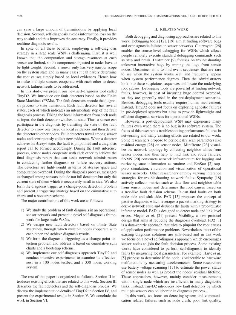
Cumulative Sum Charts: We take the traffic data as an exam-ple to illustrate the diagnosis triggering scheme. In TinyD2, weapply a window-based scheme for caching the latest parametervalues. As shown in Fig. 3(a), assume that the window size is12 and thus a sensor node stores 12 latest data points of itsingress traffic. At the first step, we calculate the cumulative sumcharts of this data sequence. Let {Xi} i = 1, 2, . . . , 12 denotethe data points in this stream and X be the mean of all values.The cumulative sums are represented as {Ci} i = 0, 1, . . . , 12.Here we define C0 = 0 and then the other cumulative sums arecalculated by adding the difference between current value andthe mean value to the prior sum.

Ci = Cj−1 + (Xi −X) (1)

The CUSUM series are illustrated in Fig. 3(b). The CUSUMreaches zero at the end. An increase of the CUSUM valueindicates that the values in this period are above the overall


Fig. 3. Cumulative sum charts.

average value and a descending curve means that values in thecorresponding period are below the overall average.

A straight line in the cumulative sum charts indicates that theoriginal values are relatively stable. In contrast, bowed curvesare caused by variations in the initial values. The CUSUM curvein Fig. 3(b) turns in direction around C6 and we can infer thatthere is an abrupt change. Besides making decision directlyaccording to the CUSUM charts, we also propose to assign aconfidence level to our determination by a bootstrap analysis.

Bootstrap Strategy: Before discussing the bootstrap scheme,we firstly introduce an estimator (Dc) of the change which isdefined as the difference between maximum value and mini-mum value in {Ci}.

Dc = max(Ci)−min(Ci) (2)

In each bootstrap, we randomly reorder the original valuesand obtain a new data sequence, that is, {Xj

i }j = 1, 2, . . .mwhere m denote the number of bootstraps we performed. Thenthe cumulative sums {Cj

i } as well as the corresponding Djc are

calculated based on the new sequence {Xji }.

The idea behind bootstrap is that randomly reordered datasequences simulate the behavior of CUSUM if no change hasoccurred. With multiple bootstrap samples we can estimate thedistribution of Dc without value changes. We then derive theconfidence level by comparing the Dc calculated from valuesin original order with that from the bootstrap samples.

Confidence = NumberOf(Dc > Djc)/m (3)

Where Dc is calculated from the original data sequenceand Dj

c is derived from a bootstrap, m is the total number ofbootstraps performed. If the confidence is above a pre-specifiedthreshold, for example 90%, we decide that there is an apparentchange in the parameter values.

Localizing the Change-Point: After determining the occur-rence of a change, we localize the position of the change witha simple strategy by finding Ci with the largest abstract value.In this example, C6 has the largest abstract value, so we decidethat the value change occurs between X6 and X7. Note thatthis method can easily be generalized to find multiple changes,however, in this work we only cache and process parametervalues in a short period, so we only pick out the major changeand trigger a diagnosis process.

TABLE IDEPLOYMENTS OF THE FOREST MONITORING PROJECT

IV. TINYD2 IMPLEMENTATION

We have implemented the TinyD2 on the Telosb mote with aMSP430 processor and CC2420 transceiver. On this hardwareplatform, the program memory is 48 K bytes and the RAMis 10 K bytes. We apply the TinyOS 2.1 as our software de-velopment platform and the application and TinyD2 diagnosisfunctionalities are implemented as different components. In thefollowing subsections, we will firstly introduce the applicationbackground and the protocol design of our GreenOrbs project,and then we show the details of integrating TinyD2 withGreenOrbs.

A. The GreenOrbs Sensor Network System

We launch our forest monitoring sensor network systemwhich targets several urgent applications in forestry such ascanopy closure estimates, carbon sequestration, research onbiodiversity and the fire risk prediction. Table I illustrates ourmain deployment experiences up to now.

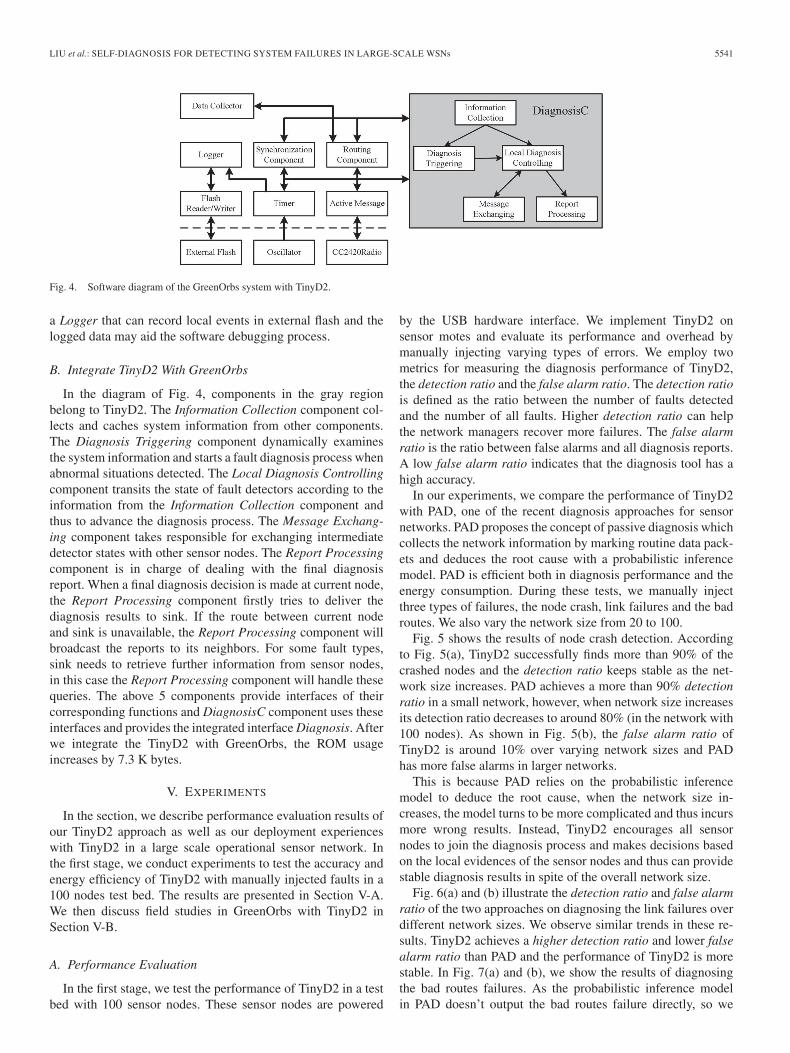
The software on the sensor nodes is developed on the TinyOS2.1 which is the most widely used platform for sensor networks.Fig. 4 illustrates the major components in our system. We applysome components from the TinyOS library which provide lowlayer functionalities such as the basic wireless communication,the timing service and methods for accessing the external flash.The Data Collector is in charge of sampling the sensing dataand sending them to sink through multi-hop routes. Our routingprotocol is design based on the CTP [3]. The SynchronizationComponent provides the network-wide synchronization serviceand thus enables the synchronized duty cycles. We also include


Fig. 4. Software diagram of the GreenOrbs system with TinyD2.

a Logger that can record local events in external flash and thelogged data may aid the software debugging process.

B. Integrate TinyD2 With GreenOrbs

In the diagram of Fig. 4, components in the gray regionbelong to TinyD2. The Information Collection component col-lects and caches system information from other components.The Diagnosis Triggering component dynamically examinesthe system information and starts a fault diagnosis process whenabnormal situations detected. The Local Diagnosis Controllingcomponent transits the state of fault detectors according to theinformation from the Information Collection component andthus to advance the diagnosis process. The Message Exchang-ing component takes responsible for exchanging intermediatedetector states with other sensor nodes. The Report Processingcomponent is in charge of dealing with the final diagnosisreport. When a final diagnosis decision is made at current node,the Report Processing component firstly tries to deliver thediagnosis results to sink. If the route between current nodeand sink is unavailable, the Report Processing component willbroadcast the reports to its neighbors. For some fault types,sink needs to retrieve further information from sensor nodes,in this case the Report Processing component will handle thesequeries. The above 5 components provide interfaces of theircorresponding functions and DiagnosisC component uses theseinterfaces and provides the integrated interface Diagnosis. Afterwe integrate the TinyD2 with GreenOrbs, the ROM usageincreases by 7.3 K bytes.

V. EXPERIMENTS

In the section, we describe performance evaluation results ofour TinyD2 approach as well as our deployment experienceswith TinyD2 in a large scale operational sensor network. Inthe first stage, we conduct experiments to test the accuracy andenergy efficiency of TinyD2 with manually injected faults in a100 nodes test bed. The results are presented in Section V-A.We then discuss field studies in GreenOrbs with TinyD2 inSection V-B.

A. Performance Evaluation

In the first stage, we test the performance of TinyD2 in a testbed with 100 sensor nodes. These sensor nodes are powered

by the USB hardware interface. We implement TinyD2 onsensor motes and evaluate its performance and overhead bymanually injecting varying types of errors. We employ twometrics for measuring the diagnosis performance of TinyD2,the detection ratio and the false alarm ratio. The detection ratiois defined as the ratio between the number of faults detectedand the number of all faults. Higher detection ratio can helpthe network managers recover more failures. The false alarmratio is the ratio between false alarms and all diagnosis reports.A low false alarm ratio indicates that the diagnosis tool has ahigh accuracy.

In our experiments, we compare the performance of TinyD2with PAD, one of the recent diagnosis approaches for sensornetworks. PAD proposes the concept of passive diagnosis whichcollects the network information by marking routine data pack-ets and deduces the root cause with a probabilistic inferencemodel. PAD is efficient both in diagnosis performance and theenergy consumption. During these tests, we manually injectthree types of failures, the node crash, link failures and the badroutes. We also vary the network size from 20 to 100.

Fig. 5 shows the results of node crash detection. Accordingto Fig. 5(a), TinyD2 successfully finds more than 90% of thecrashed nodes and the detection ratio keeps stable as the net-work size increases. PAD achieves a more than 90% detectionratio in a small network, however, when network size increasesits detection ratio decreases to around 80% (in the network with100 nodes). As shown in Fig. 5(b), the false alarm ratio ofTinyD2 is around 10% over varying network sizes and PADhas more false alarms in larger networks.

This is because PAD relies on the probabilistic inferencemodel to deduce the root cause, when the network size in-creases, the model turns to be more complicated and thus incursmore wrong results. Instead, TinyD2 encourages all sensornodes to join the diagnosis process and makes decisions basedon the local evidences of the sensor nodes and thus can providestable diagnosis results in spite of the overall network size.

Fig. 6(a) and (b) illustrate the detection ratio and false alarmratio of the two approaches on diagnosing the link failures overdifferent network sizes. We observe similar trends in these re-sults. TinyD2 achieves a higher detection ratio and lower falsealarm ratio than PAD and the performance of TinyD2 is morestable. In Fig. 7(a) and (b), we show the results of diagnosingthe bad routes failures. As the probabilistic inference modelin PAD doesn’t output the bad routes failure directly, so we


Fig. 5 (a) The detection ratio for node crash V.S. network size. (b) The falsealarm ratio for node crash V.S. network size.

Fig. 6 (a) The detection ratio for link failures V.S. network size. (b) The falsealarm ratio for link failures V.S. network size.

only present the results of TinyD2. According to the resultsin Figs. 5–7, we can conclude that TinyD2 achieves similarperformances on detecting all these three types of failures.

Fig. 7 (a) The detection ratio for bad routes V.S. network size. (b) The falsealarm ratio for bad routes V.S. network size.

Fig. 8. Overhead (TinyD2 V.S. PAD).

We then evaluate the overhead of TinyD2. We firstly comparethe traffic overhead of TinyD2 with that of PAD. PAD is verylightweight in the bandwidth consumption since it obtains net-work information only by marking routine data packets. Notethat it is difficult to directly measure the energy consumptionof the diagnosis services from an operational sensor networkwithout extra hardware. As radio communications dominate thepower consumption [22] of diagnosis approaches, we use thetraffic incurred by different diagnosis approaches to estimatetheir energy cost. We apply the ratio between diagnosis trafficand the overall network traffic to quantify the overhead. Fig. 8shows the CDF of the two approaches’ traffic overhead. TheX axis shows the percentage of traffic that a diagnosis tool takesin total network traffic and Y axis illustrates the cumulativeprobability. For example, a data point <5%, 0.9> means thatat 90% of cases the diagnosis tool takes less than 5% of the


Fig. 9. Overhead over time.

total traffic. The curve of TinyD2 is on the left of the curve ofPAD which indicates that the cumulative overhead of TinyD2 isless than PAD. For example, according to Fig. 8, at 80% of thecases the TinyD2 only uses less than 3.5% of overall networktraffic while PAD uses less than 6%. Note that typical sink-based approaches such as Sympathy [18] can incur even moretraffic cost than the initial sensory data acquisition applicationsand thus their traffic usages can exceed 50%. Reasons to ex-plain the results are three-folds. First, TinyD2 mainly exploreslocal information exchange with sporadic reports to sink andin sink-based approaches, system metrics from all nodes aredelivered to sink over long paths. Second, TinyD2 uses shortmessages, which contains the state of a detector only. Sink-based methods, however, need to transmit a large number ofparameters. Finally, in TinyD2, only the problematic regionstrigger a diagnosis process while sink-based schemes requireall nodes periodically report their information.

We also evaluate the overhead of TinyD2 over time. Asshown in Fig. 9, we find that the overhead of TinyD2 exhibitshigh variations over time. In this figure, X axis is the timelineand the Y axis shows the traffic overhead. In some timestamps,the diagnosis overhead is less than 1% and in some other times-tamps the overhead can reach to nearly 4%. This is becausethe TinyD2 is an on-demand approach which only works whennetwork failures occur.

B. Field Studies

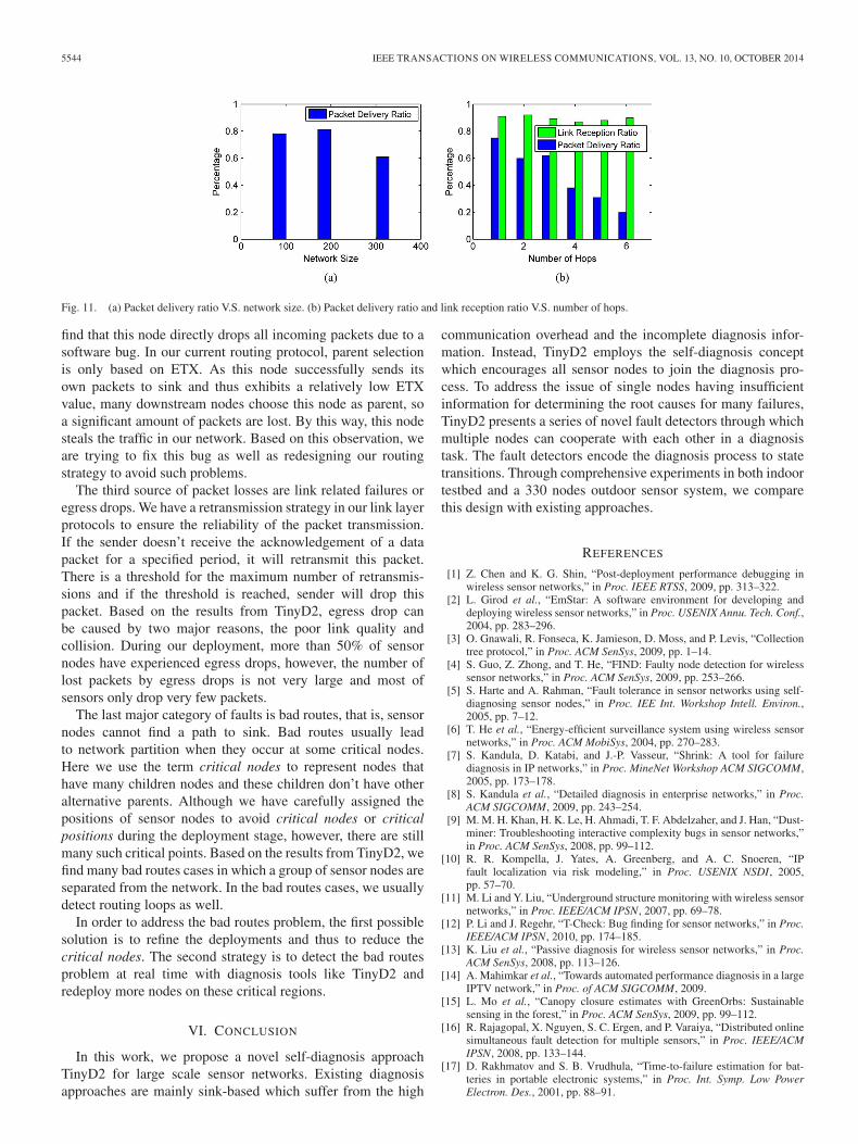
In this section, we discuss our field studies with TinyD2 inour GreenOrbs system. A part of the logical topology of ournetwork is illustrated in Fig. 10. During the deployments, wemeasure the system performance by the Packet Delivery Ratiowhich is the ratio between the number of packets received bysink and the number of packets sent by all sensor nodes. Wealso randomly sample two local metrics on some sensor nodes,the Link Reception Ratio and Traffic.

As illustrated in Fig. 11(a), when the network contains 100and 200 nodes, nearly 80% of the packets are reported tosink in time. When the network size is 330 nodes, the PacketDelivery Ratio is around 60%. Fig. 11(b) shows the averagePacket Delivery Ratio of nodes that have varying hop distancesto sink. According to the results, we can conclude that thefarther the node is away from sink, the less data they deliverto sink. Meanwhile, Fig. 11(b) also presents the average Link

Fig. 10. Part of logical topology of the forest monitoring sensor system.

Reception Ratio of nodes that have different hop distances tosink. From the results in Fig. 11(b), we find that more than90% transmissions on our sampled links can successfully reachthe receiver in varying areas of the network. Note that thecommunication protocol applied in our current system has alink layer retransmission strategy, so we believe that poor linkqualities are not the major cause of the system performancedegradation.

With the help of TinyD2, we summarize four major cat-egories of network faults that are responsible for the poorPacket Delivery Ratio in our system. We analyze the occurrencefrequency of these failures as well as their hazard rating tothe network performance. We also propose advice on potentialrecovery methods.

The first category of failures is node crash, including bothsoftware and hardware errors. The crashed nodes do not sendor respond to any message. These fatal errors are caused by theunreliability of the software system and physical damages. Forexample, the rain can short-circuit the batteries of sensor nodesand thus destroy the nodes’ power supply. Nodes that experi-ence a software crash can be recovered by manually reboot andphysical damages can only be resolved by changing the hard-ware. TinyD2 detects that around 3% of nodes may be crashedduring a long term deployment. The occurrences of node crashrandomly distribute over the whole deployment regions.

The second category of network faults are ingress dropsor message pool overflow drops. Ingress drop means that thereceiver has successfully acknowledged a packet but drops thepacket before processing it. In our current system, the receivedpackets are firstly cached in a message pool of the sensor node,and then being processed and forwarded to the parent node.If the message pool overflows, the ingress drop occurs. Themessage pool will overflow if the incoming traffic is higher thanthe node processing capability. Besides, ingress drops can alsoresult from some software bugs. According to the results fromTinyD2, only a few nodes (around 2% of all sensor nodes) havethe ingress drop problem. They, however, severely deterioratethe system performance. For example, during our deploymentone sensor nodes that experience ingress drop contributesnearly 10% of all packet losses. With further investigation, we


Fig. 11. (a) Packet delivery ratio V.S. network size. (b) Packet delivery ratio and link reception ratio V.S. number of hops.

find that this node directly drops all incoming packets due to asoftware bug. In our current routing protocol, parent selectionis only based on ETX. As this node successfully sends itsown packets to sink and thus exhibits a relatively low ETXvalue, many downstream nodes choose this node as parent, soa significant amount of packets are lost. By this way, this nodesteals the traffic in our network. Based on this observation, weare trying to fix this bug as well as redesigning our routingstrategy to avoid such problems.

The third source of packet losses are link related failures oregress drops. We have a retransmission strategy in our link layerprotocols to ensure the reliability of the packet transmission.If the sender doesn’t receive the acknowledgement of a datapacket for a specified period, it will retransmit this packet.There is a threshold for the maximum number of retransmis-sions and if the threshold is reached, sender will drop thispacket. Based on the results from TinyD2, egress drop canbe caused by two major reasons, the poor link quality andcollision. During our deployment, more than 50% of sensornodes have experienced egress drops, however, the number oflost packets by egress drops is not very large and most ofsensors only drop very few packets.

The last major category of faults is bad routes, that is, sensornodes cannot find a path to sink. Bad routes usually leadto network partition when they occur at some critical nodes.Here we use the term critical nodes to represent nodes thathave many children nodes and these children don’t have otheralternative parents. Although we have carefully assigned thepositions of sensor nodes to avoid critical nodes or criticalpositions during the deployment stage, however, there are stillmany such critical points. Based on the results from TinyD2, wefind many bad routes cases in which a group of sensor nodes areseparated from the network. In the bad routes cases, we usuallydetect routing loops as well.

In order to address the bad routes problem, the first possiblesolution is to refine the deployments and thus to reduce thecritical nodes. The second strategy is to detect the bad routesproblem at real time with diagnosis tools like TinyD2 andredeploy more nodes on these critical regions.

VI. CONCLUSION

In this work, we propose a novel self-diagnosis approachTinyD2 for large scale sensor networks. Existing diagnosisapproaches are mainly sink-based which suffer from the high

communication overhead and the incomplete diagnosis infor-mation. Instead, TinyD2 employs the self-diagnosis conceptwhich encourages all sensor nodes to join the diagnosis pro-cess. To address the issue of single nodes having insufficientinformation for determining the root causes for many failures,TinyD2 presents a series of novel fault detectors through whichmultiple nodes can cooperate with each other in a diagnosistask. The fault detectors encode the diagnosis process to statetransitions. Through comprehensive experiments in both indoortestbed and a 330 nodes outdoor sensor system, we comparethis design with existing approaches.

REFERENCES

[1] Z. Chen and K. G. Shin, “Post-deployment performance debugging inwireless sensor networks,” in Proc. IEEE RTSS, 2009, pp. 313–322.

[2] L. Girod et al., “EmStar: A software environment for developing anddeploying wireless sensor networks,” in Proc. USENIX Annu. Tech. Conf.,2004, pp. 283–296.

[3] O. Gnawali, R. Fonseca, K. Jamieson, D. Moss, and P. Levis, “Collectiontree protocol,” in Proc. ACM SenSys, 2009, pp. 1–14.

[4] S. Guo, Z. Zhong, and T. He, “FIND: Faulty node detection for wirelesssensor networks,” in Proc. ACM SenSys, 2009, pp. 253–266.

[5] S. Harte and A. Rahman, “Fault tolerance in sensor networks using self-diagnosing sensor nodes,” in Proc. IEE Int. Workshop Intell. Environ.,2005, pp. 7–12.

[6] T. He et al., “Energy-efficient surveillance system using wireless sensornetworks,” in Proc. ACM MobiSys, 2004, pp. 270–283.

[7] S. Kandula, D. Katabi, and J.-P. Vasseur, “Shrink: A tool for failurediagnosis in IP networks,” in Proc. MineNet Workshop ACM SIGCOMM,2005, pp. 173–178.

[8] S. Kandula et al., “Detailed diagnosis in enterprise networks,” in Proc.ACM SIGCOMM, 2009, pp. 243–254.

[9] M. M. H. Khan, H. K. Le, H. Ahmadi, T. F. Abdelzaher, and J. Han, “Dust-miner: Troubleshooting interactive complexity bugs in sensor networks,”in Proc. ACM SenSys, 2008, pp. 99–112.

[10] R. R. Kompella, J. Yates, A. Greenberg, and A. C. Snoeren, “IPfault localization via risk modeling,” in Proc. USENIX NSDI, 2005,pp. 57–70.

[11] M. Li and Y. Liu, “Underground structure monitoring with wireless sensornetworks,” in Proc. IEEE/ACM IPSN, 2007, pp. 69–78.

[12] P. Li and J. Regehr, “T-Check: Bug finding for sensor networks,” in Proc.IEEE/ACM IPSN, 2010, pp. 174–185.

[13] K. Liu et al., “Passive diagnosis for wireless sensor networks,” in Proc.ACM SenSys, 2008, pp. 113–126.

[14] A. Mahimkar et al., “Towards automated performance diagnosis in a largeIPTV network,” in Proc. of ACM SIGCOMM, 2009.

[15] L. Mo et al., “Canopy closure estimates with GreenOrbs: Sustainablesensing in the forest,” in Proc. ACM SenSys, 2009, pp. 99–112.

[16] R. Rajagopal, X. Nguyen, S. C. Ergen, and P. Varaiya, “Distributed onlinesimultaneous fault detection for multiple sensors,” in Proc. IEEE/ACMIPSN, 2008, pp. 133–144.

[17] D. Rakhmatov and S. B. Vrudhula, “Time-to-failure estimation for bat-teries in portable electronic systems,” in Proc. Int. Symp. Low PowerElectron. Des., 2001, pp. 88–91.


[18] N. Ramanathan et al., “Sympathy for the sensor network debugger,” inProc. ACM SenSys, 2005, pp. 255–267.

[19] T. Sookoor, T. Hnat, P. Hooimeijer, W. Weimer, and K. Whitehouse,“Macrodebugging: Global views of distributed program execution,” inProc. ACM SenSys, 2009, pp. 141–154.

[20] G. Tolle and D. Culler, “Design of an application-cooperative manage-ment system for wireless sensor networks,” in Proc. IEEE EWSN, 2005,pp. 121–132.

[21] M. Wachs et al., “Visibility: A new metric for protocol design,” in Proc.ACM SenSys, 2007, pp. 73–86.

[22] Q. Wang, M. Hempstead, and W. Yang, “A realistic power consumptionmodel for wireless sensor network devices,” in Proc. IEEE SECON, 2006,pp. 286–295.

[23] A. Woo, T. Tong, and D. Culler, “Taming the underlying challenges ofreliable multihop routing in sensor networks,” in Proc. ACM SenSys,2003, pp. 14–27.

[24] X. Y. Xiao, W. C. Peng, C. C. Hung, and W. C. Lee, “Using sensorranksfor in-network detection of faulty readings in wireless sensor networks,”in Proc. 6th ACM Int. Workshop Data Eng. Wireless Mobile Access, 2007,pp. 1–8.

[25] N. Xu et al., “A wireless sensor network for structural monitoring,” inProc. ACM SenSys, 2004, pp. 13–24.

[26] J. Yang, M. L. Soffa, L. Selavo, and K. Whitehouse, “Clairvoyant: Acomprehensive source-level debugger for wireless sensor networks,” inProc. ACM SenSys, 2007, pp. 189–203.

[27] Z. Yang, M. Li, and Y. Liu, “Sea depth measurement with restrictedfloating sensors,” in Proc. IEEE RTSS, 2007, pp. 469–478.

[28] J. Zhao, R. Govindan, and D. Estrin, “Residual energy scan for monitoringsensor networks,” in Proc. IEEE WCNC, 2002, pp. 356–362.

[29] R. Zhang, P. Ji, D. Mylaraswamy, M. Srivastava, and S. Zahedi, “Cooper-ative sensor anomaly detection using global information,” Tsinghua Sci.Technol., vol. 18, no. 3, pp. 209–219, Jun. 2013.

Kebin Liu (M’08) received the B.S. degree from theDepartment of Computer Science, Tongji University,Shanghai, China, in 2004 and the M.S. and Ph.D.degrees from Shanghai Jiao Tong University, Shang-hai, in 2007 and 2010, respectively. He is currentlyan Assistant Researcher with the School of Softwareand TNLIST, Tsinghua University, Beijing, China.His research interests include WSNs and distributedsystems.

Qiang Ma received the B.S. degree from the De-partment of Computer Science and Technology,Tsinghua University, Beijing, China, in 2009 andthe Ph.D. degree in computer science and engineer-ing from Hong Kong University of Science andTechnology, Kowloon, Hong Kong, in 2013. He isnow a Postdoctoral Researcher with the School ofSoftware, Tsinghua University. His research interestsinclude sensor networks and diagnosis.

Wei Gong received the B.S. degree from the De-partment of Computer Science and Technology,Huazhong University of Science and Technology,Wuhan, China, in 2003 and the M.S. and Ph.D.degrees from the School of Software and the De-partment of Computer Science and Technology,Tsinghua University, Beijing, China, in 2007 and2012, respectively. His research interests includeWSNs, RFID, and mobile computing.

Xin Miao received the B.S. degree from the De-partment of Computer Science and Technology,Tsinghua University, Beijing, China, in 2005 and thePh.D. degree in computer science and engineeringfrom Hong Kong University of Science and Tech-nology, Kowloon, Hong Kong, in 2013. He is cur-rently a Postdoctoral Researcher with the School ofSoftware, Tsinghua University. His research interestsinclude sensor networks and RFID.

Yunhao Liu (SM’06) received the B.S. degree fromthe Department of Automation, Tsinghua University,Beijing, China, in 1995 and the M.S. and Ph.D.degrees in computer science and engineering fromMichigan State University, East Lansing, MI, USA,in 2003 and 2004, respectively. He is currently aChang Jiang Professor and the Dean of the Schoolof Software at Tsinghua University.

Documents

Self-Diagnosis for Detecting System Failures in Large-Scale Wireless Sensor Networks