Self-creating and organizing neural networks

IEEE TRANSACTIONS ON NEURAL NETWORKS, VOL. 5, NO. 4, JULY 1994 561

Self-creating and Organizing Neural Networks Doo-I1 Choi and Sang-Hui Park, Member, IEEE

Abstract- We have developed a self-creating and organizing unsupervised learning algorithm for artificial neural networks. In this study, we introduce SCONN and SCONN2 as two versions of Self-creating and Organizing Neural Network (SCONN) algorithms. SCONN creates an adaptive uniform vector quantizer (VQ), whereas SCONN2 creates an adaptive nonuniform VQ by neural-like architecture. SCONN’s begin with only one output node, which has a sufficiently wide activation level, and the activation level decrease depending upon the time or the activation history. SCONN’s decide automatically whether to adapt the weights of existing nodes or to create a new “son node.” They are compared with two famous algorithms-the Kohonen’s Self Organizing Feature Map (SOFM) [4] as a neural VQ and the Linde-Buzo-Gray (LBG) algorithm [7] as a traditional VQ. The results show that SCONN’s have significant benefits over other algorithms.

I. ADAFTFIE VECTOR QUANTIZATION

RADITIONAL VQ’s may attempt to minimize a mean T square error (MSE) or entropic performance measure. If we know information about the pattern vector such as probability density function fz (z), optimal codebook vectors can be generated [l]. As is the general case, when we do not know this probabilistic information, we use an adaptive vector quantization (AVQ) method to estimate the fz(z) automatically. Set Sj partitions the vector space Rn into k clustering sets.

BY COMPETITIVE LEARNING

The adaptive (learning) algorithm estimates the unknown probability density function fz (z). Most neural networks using competitive learning architecture can use a neural AVQ system. Then weight vectors represent centroids of each clustering set and mean square quantization error can be expressed as

Manuscript received April 1, 1992; revised September 20, 1992. D. I. Choi was with the Department of Electrical Engineering, Yonsei

University, Seoul, Korea. He is now with Kong Ju National University, Kong Ju City, Chungnam, Korea.

S. H. Park is with the Department of Electrical Engineering, Yonsei University, Seoul, Korea.

IEEE Log Number 9205986.

where d(z, wi) denotes Euclidian distance between input vector z = (zl, zz,..., zn) and weight vector wi = (wli, w2i, . . . , w,i). As the number of the clustering set k increases, probability density function fz(z) in each cluster becomes approximately uniform. Therefore we obtain

k

If input vector z is presented randomly according to its density function, the sequence of input vectors z [t] becomes stationary and ergodic, since then the time-averaged MSE

converges with probability one to MSE as t -+ W.

Competitive learning drives weights vectors to the unknown centroids Ti that minimize MSE. More generally, E[wi] = Ti holds asymptotically as the random weights vectors w; wanders in a Brownian motion about the centroid Ti [2].

Competitive learning algorithms for artificial neural networks create an AVQ that minimizes MSE. One problem is that nodes with wi far from any input vector may never win, and therefore never learn. These are sometimes called dead nodes. They may actually be desirable if the future might bring different input patterns, but otherwise can be prevented in several ways. Kohonen’s SOFM is considered as one of the most powerful algorithms that creates topographic maps and prevent dead nodes. However, problems still remain in SOFM and we will discuss those in Section 11.

Meanwhile, classical VQ, the nodes of which have no topological relations, have been shown to converge to a local optimum [7]. But problems are in place; e.g., global optimality is hard to achieve and computational time is too long in LBG. We will discuss classical VQ in Section V.

In Sections I11 and IV we propose two versions of SCONN that provide new forms of neural VQ and harmonize optimality and topographicity.

11. ON KOHONEN’S SELF-ORGANIZING FEATURE MAP

In general, stability of competitive learning algorithms largely depends on initial random weights. At the extreme case, there can exist many dead nodes that do not learn at any case. Many ideas are proposed to remove such problems [3].

1045-9227/94$04.00 0 1994 IEEE

- ~~

562 IEEE TRANSACTIONS ON NEURAL NETWORKS, VOL. 5, NO. 4, JULY 1994

XZ x2

10.

-10.

-10. 10. x i

10.

-10.

-10. 10. x i

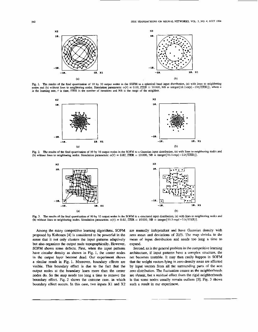
Fig. 1. The results of the final quantization of 10 by 10 output nodes in the SOFM to a spherical band input distribution, (a) with lines to neighboring nodes and (b) without lines to neighboring nodes. Simulation parameters: a(t) = 0.02, ITER = 10000, NB = integer{lO.lexp(-l5t/ITER)}, where a is the learning rate, t is time, ITER is the number of iterations and NB is the range of the neighbor.

-10. I J -10. 10. x1

X2

10. I I

-10. I I -10. 10. x i

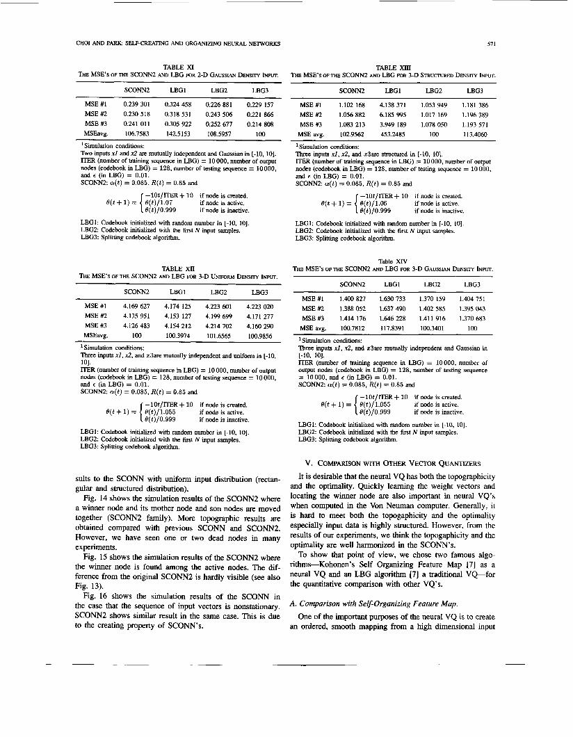
Fig. 2. (b) without lines to neighboring nodes. Simulation parameters: a(t) = 0.02, ITER = 10000, NB = integer{lO.lexp(-15t/ITER)}.

The results of the final quantization of 10 by 10 output nodes in the SoFM to a Gaussian input distribution, (a) with lines to neighboring nodes and

X t x2

10.

-10.

-10. 10. X I

10.

-10.

-10. 10. x i

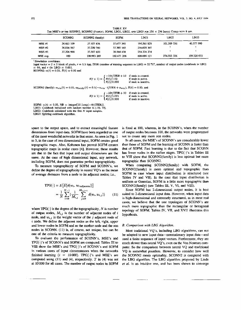
Fig. 3. The results of the final quantization of 10 by 10 output nodes in the SOFM to a structured input distribution, (a) with lines to neighboring nodes and (b) without lines to neighboring nodes. Simulation parameters: a(t) = 0.02, ITER = 10000, NB = integer{lO.lexp(-15t/ITER)}.

Among the many competitive learning algorithms, SOFM proposed by Kohonen [4] is considered to be powerful in the sense that it not only clusters the input pattems adaptively but also organizes the output node topographically. However, SOFM shows some defects. First, when the input pattems have circular density as shown in Fig. 1, the center nodes in the output layer become dead. Our experiment shows a similar result in Fig. 1. Moreover, boundary effects are visible. This boundary effect is due to the fact that the output nodes at the boundary learn more than the center nodes do. So the map needs too long a time to remove the boundary effect. Fig. 2 shows the extreme case, in which boundary effect occurs. In this case, two inputs XI and X2

are mutually independent and have Gaussian density with zero mean and deviations of 20/3. The map shr inks to the mean of input distribution and needs too long a time to expand.

Second, as is the general problem in the competitive learning architecture, if input pattems have a complex structure, the net becomes unstable. It may then easily happen in SOFM that the weight vectors lying in zero-density areas are affected by input vectors from all the surrounding parts of the non zero distribution. The fluctuation ceases as the neighborhoods are shrunk, but a residual effect from the rigid neighborhoods is that some nodes usually remain outliers [5 ] . Fig. 3 shows such a result in our experiment.

CHOI AND PARK SELF-CREATING AND ORGANIZING NEURAL NETWORKS 563

XZ

10. -1

-10.

-10. 10. x i

XZ

10. 14 -10.

_______~

-10. 10. x i

(a) (b)

Fig. 4. The results of the final quantization of 10 by 10 output nodes in the SOFM to a nonstationary input sequence, (a) with lines to neighboring nodes and (b) without lines to neighboring nodes. The input sequence is generated at the random position in the big rectangle when t < 5000, and then in the small rectangle when 5000 < t < 10000. Simulation parameters: u(t) = 0.02, ITER = 10000, NB = integer{lO.lexp(-15t/ITER)}.

X 2 XZ

10.

-10.

-10. 10. X I

10.

-10.

-10. 10. x i (a) (b)

Fig. 5. and (b) without lines to neighboring nodes. Simulation parameters: u(t) = 0.02, ITER = 10000, NB = integer{l0.lexp(-l5t/ITER)}.

The results of the final quantization of 10 by 10 output nodes in the SOFM to a rectangular input distribution, (a) with lines to neighboring nodes

TABLE I AN ALGORITHM FOR THE ScO"

Step 1. Initialize weights. Step 2. Present new input. Step 3. Step 4. Select winner node. Step 5.

Calculate distance to all node@).

Decide whether winner node is active. If winner node is active, then go to step 6. If winner node is inactive, then go to step 7. Adapt weights of active winner node (or winner node and its family nodes). Decrease activation values of all nodes. Go to step 2.

Step 6.

Fig. 6. Learning in tree topology.

Step 7. Create a son node from an inactive winner (mother) node. Decrease activation values of all nodes. Go to step 2.

Third, SOFM can not overcome the so-called stability- plasticity dilemma; i.e., the weight vector set can not adapt neatly to new input regions in the case where the sequence of input vectors are nonstationary. Fig. 4 shows such a result in our experiment. This result is due to change in the input environment after the neighbor is rigid.

On the other hand, if the input vector distribution is more uniform, e.g., the rectangular distribution of Fig. 5, the weight vectors set neatly adapts to the input data.

111. THE SELF CREATING AND ORGANIZING NEURAL NETWORK

We assumed that there are a few neurons at the primitive stage and that stimuli that activate the neurons have a wide dynamic range-i.e., the neuron's activation levels are large

enough to be activated for any input stimuli. Suppose that the activation levels of all the neurons decrease slowly to a certain level as time goes by; then there can be a neuron that is the most stimulated but not active on a certain input stimulus. We assumed one more thing-that a most stimulated (but not active) neuron creates a son neuron to resemble itself. The details of SCONN algorithm is presented in Table I.

At the first step, it is assumed that there is only one output node with small random weight at the primitive stage (i.e., j = 0) and its activation level is set large enough to respond to any input stimuli. At the second step, new input is presented randomly or sequentially.

At the third step, distance(s) d3 between the input and each output node j is (are) calculated using (5).

N-I

dj" = (xi(t) - wi,j(t))' i = O

( 5 )


o P cell a1 0 0 1 1 1 2

0 x1 x2

'I1 1

(a)

(C) (d)

Fig. 7. The concept of the various stages in the SCONN, where two input vectors X1 and X2 are uniformly distributed in the box. Small circles indicate weight vectors and large circles indicate activation levels; i.e., (a) is for the primitive stage of the SCONN, where the activation level of a P cell is so wide that it creates no son cells, and (b) is for the creating stage of the SCONN, where the P cell creates a son cell because of a decreasing activation level, (c) is for the organizing stage of the SCONN, where weight vectors converge to its own region and (d) is for the final stage of the SCONN, where input vectors are clustered uniformly.

XZ

10.

-10.

XZ

10.

x2

10.

-10.

-10. 10. X I -10. 10. x i

-10.

-10. 10. X I -10. 10. x1

(C) ( 4 Fig. 8. Weight vectors during the creating and organizing process. (a) t = 0, (b) t = 400, (c) t = 2000 and (d) t = 10000.

where zz(t) is the input to node i at time t and ~ , , ~ ( t ) is the weight from input node i to output node j at time t. At the fourth step, an output node with the minimum distance is selected as the winner. At the fifth step, it is decided using (6) whether the winner node is active or inactive.

YW3 ( is inactive, otherwise

where yw3 is the output of the winner node, d,, is the distance between the inputs and the winner node, and O(t) is an activation level that is sufficiently wide at a primitive stage and decreases with time.

At the sixth step, the weights of an active winner node is adapted using (7)

(6 ) is active, if dw3 < O(t)

w, w,(t + 1) = %, w,(t) + (.ll(t)(G(t) - wz, w,(t)) (7)

CHOI AND PARK: SELF-CREATING AND ORGANIZING NEURAL NETWORKS 565

X2

-10. 10. xi

(a) X 2

10 .1 . . . . . . . . .1 . m . .. . . . . I ..

...... . . . . . . . . . . . . .

m . 9 .

W . . 1. . 9 . . ..... . .. . ........ -10. 10. xi

(b)

Fig. 9. The results of the final quantization of 100 output nodes in the SCONN to a rectangular input distribution, (a) with lines between mother nodes and son nodes and (b) without lines between mother nodes and son nodes. Simulation parameters: a(t) = 0.085, ITER = 10000, R(t) = 0.85, and 19(t) = 8.5exp(-O.O01t)+ 1.5, where a is the learning rate, t is time, ITER is the number of iterations, R is the resemblance factor, and I9 is the activation level.

XZ

10.

-10.

-10. 10. xi

(a) XZ

Fig. 10. The results of the final quantization of 100 output nodes in the SCONN to a structured input distribution, (a) with lines between mother nodes and son nodes and (b) without lines between mother nodes and son nodes. Simulation parameters: a(t) = 0.085, ITER = 10000, R(t) = 0.85, and O ( t ) = 9exp(-O.O01t) + 1.

X2

10.

-10.

-10. 10. xi

(a) X2

10.

-10.

. . .. ........ ......... m 8.. , . . 8 ". S', ' ...... :.-. . = : . . . .

-10. 10. xi

(b)

Fig. 11. The results of the final quantization of 100 output nodes in the SCONN to a Gaussian input distribution, (a) with lines between mother nodes and son nodes and (b) without lines between mother nodes and son nodes. Simulation parameters: a(t) = 0.085, ITER = 10000, R(t) = 0.85, and O ( t ) = 8.5exp(-O.O0lt) + 1.5.

TABLE II AN ALGORITHM FOR THE SCONN2

Step 1. Step 2. Step 3. Step 4.

Step 6.

Step I .

Step 8.

step 5.

Initialize weights. Present new input. Calculate distance to all node(s). Find active node(s) and a winner node. If active node does not exist, then go to step 8. Decrease response ranges of active node(s). Increase response ranges of inactive node(s). Adapt weights of winner node (or winner node and its family nodes). Go to step 2. Create a son node from an inactive winner (mother) node. Go to step 2.

INPUT VECTOR /

A node

Fig. 12. U Altemative method to find a winner node.

where wi, wj(t) are the weights from the inputs to an active winner node and a(t) is the gain term that can be constant or decrease with time.


XZ XZ

10. I‘ 10. ,- XZ

10. r-1

-10.

-10. 10. x i

(a)

-10. 10. x i -10. 10. X I

(b) (C)

Fig. 13. The results of the final quantization of 100 output nodes in the SCONN2 to a Gaussian input distribution, (a) with lines between mother nodes and son nodes, (b) without lines between mother nodes and son nodes, and (c) with circles that indicate activation levels. Simulation parameters: a(t) = 0.085, ITER = 10 000, R(t ) = 0.85, and O ( t + 1) = -1Ot/ITER + 10 if node is created. O(t)/1.05 if node is active. O(t)/O.999 if node is inactive.

TABLE JII THE MSE’s AND TOFOGRAPHICITIES OF THE SCONN, SCONN2, SCONN2 (FAMILY LEARNING) AND SOFM FOR THE 2-D UNIFORM DENSITY INPUT.’

SCONN SCO“2 SCONN2 (family) SOFM

MSE TPG MSE TPG MSE TPG MSE TPG

1 0.699 766 2.423 679 0.692 823 2.510 171 0.730 402 2.009 671 0.808 734 1.937 326 2 0.697 004 2.419 227 0.696 019 2.379 536 0.747 959 1.919 486 0.811 306 1.991 037 3 0.707 671 2.431 449 0.701 286 2.451 331 0.761 428 1.942 320 0.801 768 1.989 436

Avg. 100.6848 123.8931 100 125.0288 107.1603 100 115.8689 100.7889

Simulation conditions: Two inputs x1 and 1 2 are mutually independent and uniform in [-lo, lo]. ITER = 10 000. Number of output nodes = 100.

SCONN2: a(t) = 0.085, R(t) = 0.85, and SCONN: a(t) = 0.085, R(t) = 0.85, and O ( t ) = 8.5exp(-O.O01t) + 1.5

-10tIITER + 10 if node is created.

if node is inactive. e( t + 1) = e(t)/ i .os if node is active. { O(t)/0.999

SCONN2 (family): awln(t) = 0.085, afam,ly(t) = 0.5(-awln . t/ITER+ aW,,), R(t) = 0.85, and

-lOt/ITER + 10 if node is created.

if node is inactive. e(t + 1) = e(t)/ i .o4 if node is active. { O(t)/0.999

SOFM: a(t) = 0.02 and NB = integer { 10.1 exp(-lBt/ITER)) where a is the learning rate, t is time, ITER is the number of iterations, R is the resemblance factor, O is the activation level, and NE! is the range of the neighborhood.

If one wants the network organized more topographically, winner node and its “family nodes” (e.g.. its mother node and son nodes) can be moved together (see Fig. 6). The amount of movement is the fraction awin and af,,;l,(t).

But this type of learning may make some nodes dead. Other adapting equations found in the literature ([2], [4], and [ 5 ] ) are also available for fine clustering.

At the seventh step, a son node is created from a mother node (an inactive winner node) using (8) and (9). The son node resembles its mother node by (9).

where s j is the current number of total output nodes, wi+j

are the weights from the inputs to a son node created from a mother node, and R(t) is the resemblance factor that varies from 0 to 1.

In this algorithm, there can be three criteria to stop the program. Those criteria are iterations ( t ) , number of output nodes ( s j ) and activation level (O(t)).

In order for a network to search for the optimal number of output nodes automatically, it is desirable to have the activation level be a criterion to stop the program. ‘ Fig. 7 shows the concept of self-creating and organizing.

To make it easier to understand, suppose that inputs $1 and 22 have uniform distributions from 0 to 1, a primitive neuron has an activation level that is greater than 1.414, and weights between neuron and input neurons are initialized randomly from 0 to 1. If activation level decreases very slowly, weight vectors of a primitive neuron move to the mean of the input

CHOI AND PARK: SELF-CREATING AND ORGANIZING NEURAL NETWORKS

X2

18.

-18.

561

X 2

18.

-18.

-18. 10. X I -10. 10. X I

(a) (b)

Fig. 14. The results of the final quantization of 100 output nodes in the SCONN2 with a topologically defined family (SCONN2(family)), to a structured input distribution (a) with lines between mother nodes and son nodes and (b) without lines between mother nodes and son nodes. Simulation parameters: awin(t) = 0.085, afamily(t) = 0.5(-awi,t/ITER + aWin), ITER = 10000, R ( t ) = 0.85, and 8( t + 1) = -lOt/ITER + 10 if node is created. 8(t)/ l .04 if node is active. 8(t) /0.999 if node is inactive.

TABLE IV THE MSE's AND TOP~GRAPHIC~~IES OF THE SCONN, SCONN2, SCONN2 (FAMILY LEARNING) AND SOFM FOR 2-D STRUCTURED DENSITY INPUT.'

~~

SCONN scoNN2 ~~

SCONN2 (family) SOFM


1 0.293 634 1.650 631 0.305 167 1.627 870 0.323 474 1.354 122 0.408 377 1.697 329 2 0.300 297 1.583 279 0.297 496 1.616 888 0.330 515 1.412 182 0.420 420 1.711 846 3 0.303 075 1.663 696 0.296 630 1.599 724 0.344 911 1.384 317 0.415 300 1.675 941

Avg. 100. 117.9970 100.2549 116.7170 111.3592 100. 138.6942 122.5146

Simulation conditions: Two inputs 21 and 12 are structured in [-lo, 101. ITER = 10000. Number of output nodes = 100. S C O W a(t) = 0.085, R(t) = 0.85, and 8( t ) = 9exp(-O.O01t) + 1. SCONN2: a(t) = 0.085, R(t) = 0.85, and


if node is inactive. 8 ( t + 1) = 8(t)/ l .05 if node is active. { 8(t) /0.999

SCONN2 (family): awin(t) = 0.085, afamily(t) = 0.5(-awin . t/ITER + a,in), R( t ) = 0.85, and

f -lOt/ITER+ 10 if node is created. 8( t + 1) = 8 ( t ) / i . 0 4 I fqt)/0.999

SOFM: a(t) = 0.02 and NE3 = integer {10.1exp(-15t/ITER)}.

vectors. Fig. 7(a) shows such a primitive stage of SCONN, where input vectors are distributed uniformly in a box. In this figure, a large circle indicates the activation level of a primitive neuron (P cell). And the weight vectors of a P cell converges to the mean of the input vectors as the learning continues, but the P cell does not create any son neurons at the primitive stage.

With the decreasing of a primitive neuron's activation level, it is possible for it to create its son neuron. Fig. 7(b) shows such a creating stage of the SCONN.

After the first creating stage, all the neurons compete with each other, so that each neuron's weight vectors converge to the mean of its own input region. Fig. 7(c) shows such an organizing stage of the SCONN. The creating stages and the organizing stages are repeated in the SCONN so that input patterns are clustered uniformly as shown in Fig. 7(d). Fig. 8 shows an example of the creating and organizing process in the SCONN with the structured input distribution,

if node is active. if node is inactive.

where a mother node and a son node are connected with lines.

Fig. 9 to Fig. 11 shows simulation results of SCONN with rectangular, structured, and Gaussian input distributions. The SCONN removes the problems of SOFM and it clusters the input patterns neatly. Moreover, under the same condition, the ability to learn in SCONN is about 1.5 times faster than in SOFM.

IV. ADAFTIVE NONUNIFORM VECTOR QUANTIZATION BY SCONN (SCONN2)

The SCONN is one of the adaptive uniform VQ's created by neural-like architecture. The nonuniform quantization is desirable in most applications because of low MSE. Now we introduce the second version of SCONN (SCONN2) which is one of the adaptive nonuniform VQ's and is easily modified from the first version of SCONN.

568

x2

10.

-10.

IEEE TRANSACTIONS ON NEURAL NETWORKS, VOL. 5 , NO. 4, JULY 1994

XZ

10.

-10.

-10. 10. xi -10. 10. xi

Fig. 15. The results of the final quantization of 100 output nodes in the SCONN2 where winner node is found among the active nodes (a) for the Gaussian input distribution and (b) for the structured input distribution. Simulation parameters: a(t) = 0.085, ITER = 10 000, R(t) = 0.85, and O(t+ l ) = -1Ot/ITER+10 if node is created. B(t)/1.05 if node is active. O(t)/O.999 if node is inactive.

XZ XZ

Fig. 16. The results of final quantization of 100 output nodes in the SCONN to a nonstationary input sequence, (a) with lines between mother nodes and son nodes, (b) without lines between mother nodes and son nodes. The input sequence is generated at the random position in the big rectangular when t < 5000, and then in the small rectangular when 5000 < t < 10000. Simulation parameters: a(t) = 0.085, ITER = 10000, R(t) = 0.85, and O ( t ) = 9.2exp(-O.O01t) + 0.8.

TABLE V THE MSE'S AND TOPOGRAPHICITIES OF THE SCoI", sCoNN2, sCo"J2 (FAMILY LEARNING) AND SoFM FOR THE 2-D GAUSSIAN DENSITY

SCONN SCONN2 SCONN2 (family) SOFM


1 0.490 871 1.869 469 0.275 424 1.572 361 0.300 301 1.212 188 0.440 644 1.102 191 2 0.488 475 1.850 346 0.279 633 1.593 742 0.305 755 1.186 630 0.391 795 1.150 293 3 0.460 356 1.897 384 0.294 822 1.591 780 0.296 966 1.156 OOO 0.449 203 1.124 921

Avg. 169.4008 166.3170 100 140.8740 106.2531 105.2529 150.8030 100

'Simulation conditions: Two inputs zl and 22 are mutually independent and Gaussian in [-lo, lo]. ITER = 10000. Number of output nodes = 100. SCO": a(t) = 0.085, R(t) = 0.85, and O ( t ) = 8.5exp(-O.O01t) + 1.5 SCONN2: a(t) = 0.085, R(t) = 0.85, and

-lOt/ITER+ 10 if node is created. if node is active. if node is inactive.


S O M . a( t ) = 0.02 and NB = integer{lO.lexp(-15t/ITER)}.

In many cases, no closed-form solution for the optimal placement of wi is possible. However, in the limit of a very large number N of quantization levels, asymptotic results can

be obtained. One quantity of chief interest is the point density function f (w) of the weight vectors in the space of the input vectors. With the distortion measure (2), the asymptotic point

CHOI AND PARK SELF-CREATING AND ORGANIZING NEURAL NETWORKS 569

TABLE VI THE MSE's AND TOW GRAPHIC^ OF THE SCONN. SCONN2. SCONN2 (FAMILY LEARNING) AND SOFM EOR 3-D UNIFORM DENSITY INPUT.

SCONN scoNN2 SCONN2 (family) SOFM


1 4.888 767 4.823 085 4.845 221 4.917 696 5.119 826 3.893 846 5.889 933 4.088 605 2 4.915 354 4.733 254 4.911 867 4.845 108 5.044 287 4.080 308 5.905 648 3.829 795 3 4.947 878 4.965 981 4.946 740 4.776 528 5.086 391 4.108 342 6.064 101 3.952 243

Ave. 100.3276 122.3381 100 122.4814 103.7179 101.7847 121.4628 100

'Simulation conditions: Three inputs cl, 22, and 23 are mutually independent and uniform in [-lo, 101. ITER = 10000. Number of output nodes = 100. SCONN: a(t) = 0.085, R(t) = 0.85, and O ( t ) = 6.3exp(-O.O01t) + 3.7. SCONN2: a(t) = 0.085, R(t) = 0.85, and

-lOt/ITER+ 10 if node is created.

if node is inactive. O ( t + 1) = O(t)/l.04 if node is active. { e(t)/o.999

SCONN2 (family): awin(t) = 0.085, afamily(t) = 0.5(-awi,. t/ITER+ awin), R(t) = 0.85, and

-1OtIITER + 10 if node is created.

if node is inactive. O ( t + 1) = O(t)/l.03 if node is active. { O(t)/0.999

S O W a(t) = 0.02 and NB = integer{ 10.1 exp(-l5t/ITER)}.

TABLE W THE MSE'S AND TOP~GRAPHICITIES OF THE SCONN, sCoNN2, sCoNN2 (FAMILY LEARNING), AND SoFM FOR 3-D STRUcnrrtED DENSITY

SCONN scoNN2 SCONN2 (family) SOFM


1 1.204 077 3.022 673 1.297 048 2.929 170 1.426 308 2.585 696 2.325 819 3.986 451 2 1.178 982 3.033 456 1.272 655 2.990 427 1.402 380 2.575 390 2.397 905 4.266 053 3 1.192 455 2.998 349 1.319 378 3.031 778 1.330 718 2.500 069 2.415 691 4.231 573

Ave. 100 1 18.1869 108.7698 116.841 1 116.3303 100 199.6752 162.9529

'Simulation conditions: Three inputs 21, 22, and 23 are structured in [-lo, 101. ITER = 10000. Number of output nodes = 100. SCO": a(t) = 0.085, R(t) = 0.85, and O ( t ) = 12exp(-O.O01t) + 2. SCONN2: a(t) = 0.085, R(t) = 0.85, and



SCONN2 (family): a,in(t) = 0.085, afamily(t) = 0.5(-a,jn . t/ITER+ awin). R(t) = 0.85, and

-1OtIITER + 10 if node is created.


SOFM: a( t ) = 0.02 and NB = integer{l0.lexp(-l5t/ITER)}.

density f (w) has been shown to be

f (w) = const. . f ( z ) 4 ( m + 2 )

Therefore the algorithm of the SCONN2 is changed from that of SCONN as shown in Table 11.

At the fourth step in the algorithm given in Table 11, there can be two methods to find a winner node. These are to find a winner node among the whole nodes or the active nodes. To find a winner node among the active nodes is realistic. However, as shown in Fig. 12, it is possible that the node (B node in Fig. 12) that is the nearest to the input vector

(A node in Fig. 12) moves toward the input vector. Although this phenomenon scarcely occurs and is negligible, it can affect the stability of the network. We think that in practice

if N + (10)

where n denotes the quantization dimension [6]. In the SCONN, activation levels of all the node decrease

with time, so that weight vectors are distributed at the final stage according to the input distribution. One idea of

sampled input then the activation levels of that nodes decrease and the activation levels of other nodes increase to estimate e($) according to (10) automatically.

nonunifom AVQ is that if the nodes are active on a certain is not active, SO that another node far from the input Vector

570 IEEE TRANSACTIONS ON NEURAL NETWORKS, VOL. 5 , NO. 4, JULY 1994

TABLE VIII Tm MSE's AND TOPOGRAPHIC^ OF THE SCONN, SCONN2, SCONN2 (FAMILY LEARNING) AND SOFM FOR 3-D GAUSSIAN DENSITY h".'

SCONN SCONN2 SCONN2 (family) SOFM

MSE TPG MSE TPG MSE TPG MSE TPG ~ ~

1 1.771 797 3.101 582 1.671 795 2.856 377 1.721 856 2.181 352 1.959 929 2.061 715 2 1.785 820 3.046 252 1.679 738 2.863 404 1.658 060 2.237 052 2.018 215 2.023 421 3 1.773 733 3.128 836 1.624 331 2.831 346 1.696 961 2.146 209 1.990 817 1.962 037

Avg. 107.1440 153.4051 100 141.4070 102.0301 108.5567 119.9583 100

' Simulation conditions: Three inputs 11, 22, and 23 are mutually independent and Gaussian in [-lo, 101. ITER = 10000. Number of output nodes = 100. SCONN: a(t) = 0.085, R(t ) = 0.85, and O ( t ) = 7.6exp(-O.O01t) + 2.4. SCONN2: a(t) = 0.085, R(t) = 0.85, and


if node is inactive. e( t + 1) = e(t)/i.o35 if node is active. { e ( t ) / o . m g

SCONN2 (family): awin(t) = 0.085, afamily(t) = 0.5(-awin . t/ITER + aWin), R(t) = 0.85, and


if node is inactive. e( t + 1) = e(t)/i.o25 if node is active. { e ( t ) /o .wg

SOFM: a(t) = 0.02 and NB = integer{lO.lexp(-15t/ITER)}.

X2 X2 XZ

10.

-10.

10.

-10.

10.

-10.

-10. 10. x1 -18. 10. x1 -10. 10. x i (a) (b) (C)

Fig. 17. The results of the final quantization of 128 codebook vectors in the LBG algorithm to a structured input distribution. (a) Codebook vectors are initialized randomly. (b) The first N vectors in the training sequence are chosen as the initial codebook vectors. (c) The splitting algorithm. Simulation conditions: Number of training sequence: 1OOOO. Number of codebook vectors: 128. If (MSEm-l - MSE,)/MSE, 5 0.001, halt.

TABLE M TABLE X W MSE's OF THE SCONN2 AND LBG FOR 2-D UNIFORM DENSITY hpur.l Tm MSE's OF THE SCONN2 AND LBG FOR 2-D STRUCTURED DENSITY INPUT.

SCONN2 LBGl LBG2 LBG3 SCONN2 LBGl LBG2 LBG3

MSE #1 0.558 600 0.565 759 0.542 449 0.547 332 MSE #1 0.235 704 0.333 789 0.301 716 0.307 404 MSE #2 0.550 864 0.536 535 0.540 349 0.541 463 MSE #2 0.232 621 0.353 793 0.258 982 0.245 014 MSE #3 0.550 087 0.570 425 0.551 344 0.558 001 MSE #3 0.235 315 0.359 937 0.263 412 0.248 063

MSE avg. 101.5549 102.3607 100 100.7744 MSE avg. 100 148.8714 117.1210 113.7629

' Simulation conditions: Two inputs XI and x2 are mutually independent and uniform in [-lo, 101. ITER (number of training sequence in LBG) = 10 000, number of output nodes (codebook in LBG) = 128, number of testing sequence = 10000, and E (in LBG) = 0.01. SCONN2: a(t) = 0.085, R(t) = 0.85 and

' Simulation conditions: ' h o inputs XI and x2 are structured in [-lo, 101. ITER (no. of training sequence in LBG) = 10 000, number of output nodes (codebook in LBG) = 128, number of testing sequence = 10000, and E (in LBG) = 0.01. SCONN2: a(t) = 0.085, R(t) = 0.85 and

-lOt/ITER + 10 if node is created. if node is active. if node is inactive.

-10t/ITER + 10 if node is created. if node is active. if node is inactive.

LBG1: Codebook initialized with random number in [-lo, 101. LBG2: Codebook initialized with the first N input samples. LBG3: Splitting codebook algorithm.

LBG1: Codebook initialized with random number in [-lo, 101. LBG2 Codebook initialized with the first N input samples. LBG3: Splitting codebook algorithm.

finding a winner node among the whole nodes is the better method.

Fig. 13 shows the simulation results of the SCONN2 with Gaussian input distribution. The SCONN2 shows similar re-


TABLE XI TABLE XIII THE MSE's OF THE SCONN2 AND LBG FOR 2-D GAUSSIAN DENSITY INPUT. THE MSE's OF THE SCONN2 AND LBG FOR 3-D STRUCTURED DENSITY INPUT.

SCONN2 LBGl LBG2 LBG3

MSE #1 0.239 301 0.324 458 0.226 881 0.229 157 MSE #2 0.230 518 0.318 531 0.243 506 0.221 866 MSE #3 0.241 011 0.305 922 0.252 677 0.214 808 MSEavg. 106.7583 142.5153 108.5957 100

'Simulation conditions: ' b o inputs XI and x2 are mutually independent and Gaussian in [-IO, 101. ITER (number of training sequence in LBG) = 10 000, number of output nodes (codebook in LBG) = 128, number of testing sequence = 10 000, and E (in LBG) = 0.01. SCONN2: a(t) = 0.085, R(t) = 0.85 and


if node is inactive.

LBGl: Codebook initialized with random number in [-lo, 101. LBG2 Codebook initialized with the first N input samples. LBG3: Splitting codebook algorithm.

e( t + 1) = q t ) / i . 0 7 if node is active. { O(t)/0.999

TABLE XII THE MSE's OF THE SCONN2 AND LBG FOR 3-D UNIFORM DENSITY INPUT.

~ ~~

SCONN2 LBGl LBG2 LBG3 ~~

MSE #1 4.169 627 4.174 125 4.223 601 4.223 020 MSE #2 4.135 951 4.153 127 4.199 699 4.171 277 MSE #3 4.126 483 4.154 212 4.214 702 4.160 290 MSEavg. 100 100.3974 101.6565 100.9856

~ ~~ ' Simulation conditions: Three inputs XI, x2, and z3are mutually independent and uniform in [-lo, 101. ITER (number of training sequence in LBG) = 10 000, number of output nodes (codebook in LBG) = 128, number of testing sequence = 10 000, and E (in LBG) = 0.01. SCONN2 a(t) = 0.085, R(t) = 0.85 and



LBGl: Codebook initialized with random number in [-lo, 101. LBG2: Codebook initialized with the first N input samples. LBG3: Splitting codebook algorithm.

O ( t + 1) = O(t)/1.055 if node is active. { e(t)/o.999

sults to the SCONN with uniform input distribution (rectangular and structured distribution).

Fig. 14 shows the simulation results of the SCONN2 where a winner node and its mother node and son nodes are moved together (SCONN2 family). More topographic results are obtained compared with previous SCONN and SCONN2. However, we have seen one or two dead nodes in many experiments.

Fig. 15 shows the simulation results of the SCONN2 where the winner node is found among the active nodes. The dif- ference from the original SCONN2 is hardly visible (see also Fig. 13).

Fig. 16 shows the simulation results of the SCONN in the case that the sequence of input vectors is nonstationary. SCONN2 shows similar result in the same case. This is due to the creating property of SCONN's.

SCONN2 LBGl LBG2 LBG3

MSE #1 1.102 168 4.138 371 1.053 949 1.181 386 MSE #2 1.056 882 6.185 995 1.017 169 1.196 389 MSE #3 1.083 213 3.949 189 1.078 050 1.193 571

MSE avg. 102.9562 453.2485 100 113.4060

'Simulation conditions: Three inputs x l , x2, and z3are structured in [-lo, lo]. ITER (number of training sequence in LBG) = 10000, number of output nodes (codebook in LBG) = 128, number of testing sequence = 10000, and E (in LBG) = 0.01. SCONN2: a(t) = 0.085, R(t) = 0.85 and



LBG1: Codebook initialized with random number in [-lo, 101. LBG2: Codebook initialized with the first N input samples. LBG3: Splitting codebook algorithm.

O ( t + 1) = O(t)/1.06 if node is active. { e ( t ) /o .wg

Table XIV THE MSE's OF THE SCONN2 AND LBG FOR 3-D GAUSSIAN DENSITY INPUT.

SCONN2 LBGl LBG2 LBG3 _____ ~ ~ _ _ _ _ _ ~~ _____

MSE #1 1.400 827 1.630 733 1.370 159 1.404 751 MSE #2 1.388 052 1.637 490 1.402 585 1.395 043 MSE #3 1.414 176 1.646 228 1.411 916 1.370 683

MSE avg. 100.7812 117.8391 100.3401 100

' Simulation conditions: Three inputs XI , x2, and 23are mutually independent and Gaussian in [-lo, 101. ITER (number of training sequence in LBG) = 10000, number of output nodes (codebook in LBG) = 128, number of testing sequence = 10000, and e (in LBG) = 0.01. SCONN2: a(t) = 0.085, R(t) = 0.85 and


LBG1: Codebook initialized with random number in [-lo, 101. LBG2 Codebook initialized with the first N input samples. LBG3: Splitting codebook algorithm.

v. COMPARISON WITH OTHER VECMR QUANTIZERS

It is desirable that the neural VQ has both the topographicity and the optimality. Quickly learning the weight vectors and locating the winner node are also important in neural VQ's when computed in the Von Neuman computer. Generally, it is hard to meet both the topogaphicity and the optimality especially input data is highly structured. However, from the results of our experiments, we think the topogaphicity and the optimality are well harmonized in the SCONN's.

To show that point of view, we chose two famous algorithms-Kohonen's Self Organizing Feature Map [7] as a neural VQ and an LBG algorithm [7] a traditional VQ-for the quantitative comparison with other VQ's.

A . Comparison with Self-organizing Feature Map. One of the important purposes of the neural VQ is to create

an ordered, smooth mapping from a high dimensional input

IEEE TRANSACITONS ON NEURAL NETWORKS, VOL. 5, NO. 4, JULY 1994 512

TABLE XV Re MSES OF THE SCONN2, SCONN2 ( F ~ Y ) , SOFM, LBG1, LBG2, AND LBG3 FOR 256 X 256 IMAGE CODED WITH 8 BPP.

SCONN2 SCONN2 (family) SOFM LBGl LBG2 LBG3

MSE #1 36.663 109 37.107 838 37.677 395 194.561 829 101.389 336 40.377 960 MSE #I2 36.836 567 37.200 760 37.303 165 216.039 307 MSE #3 37.306 988 37.587 650 38.564 438 254.334 274

109.320 023 MSE ave. 100 100.983 269 102.471 268 600.086 121 274.503 326

Simulation conditions: Input vector = 2 x 2 block of pixels, r = 1.5 bpp, ITER (number of training sequence in LBG) = 32 767, number of output nodes (codebook in LBG) = 64, and E (in LBG) = 0.001. SCONN2: a(t) = 0.05, R ( t ) = 0.95 and


if node is inactive. O ( t + 1) = O(t)/l.02 if node is active.

SCONN2 (family): a,;,(t) = 0.05, afamily(t) = 0.5(-aW;,. t/ITER + awin), R(t ) = 0.95, and

-10t/ITER+ 10 if node is created. O(t + 1) = O(t)/l.015 if node is active.


{ e( t)/0.999

{ O(t)/0.999

SOFM: a(t) = 0.05, NB = integer{lO.lexp(-4t/lTER)}. LBGI: Codebook initialized with random number in [-lo, 101. LBG2: Codebook initialized with the first N input samples. LBG3: Splitting codebook algorithm.

space to the output space, and to extract meaningful feature dimensions from input data. SOFM have been regarded as one of the most wonderful networks in that sense. As seen in Fig. 1 to 5, in the case of two dimensional input, SOFM creates good topographic maps. Also, Kohonen has proved SOFM creates topographic maps in scalar cases [4]. However, these results are due to the fact that input and output dimensions are the same. At the case of high dimensional input, any network, including SOFM, does not guarantee perfect topographicity.

To measure topographicity of SOFM and SCONN’s, we define the degree of topographicity in neural VQ’s as the mean of average distances from a node to its adjacent nodes; i.e.,

where TPG(-) is the degree of the topographicity, N is number of output nodes, M i j is the number of adjacent nodes of i node, and wi,j is the weight vector of the j adjacent node of i node. We define the adjacent nodes as the left, right, upper and lower nodes in SOFM and as the mother node and the son nodes in SCONN. (1 1) is, of course, not unique, but can be one of the criteria to measure topographicity.

To evaluate the performance of SCONN’s, MSE’s and TPG(-)’s of SC0N”s and SOFM are computed. Tables I11 to VI11 show the MSE’s and TPG(.)’s of SC0N”s and SOFM in various cases of input circumstances when the networks finished learning (t = 10000). TPG(.)’s and MSE’s are computed using (11) and (4), respectively. T in (4) was set at loo00 for all cases. The number of output nodes in SOFM

is fixed at 1 0 0 , whereas, in the SCONN’s, when the number of output nodes becomes 1 0 0 , the networks were programmed not to create any more son nodes.

In all cases, the MSE’s of SCONN’s are considerably lower than those of SOFM and the learning of SCONN is faster than that of SOFM. Fast learning is due to the fact that SCONN has fewer nodes in the earlier stages. TPG(-)’s in Tables I11 to VIII show that SCONN2(family) is less optimal but more topographic than SCONN2.

When comparing SCONN2(family) with SOW, the SCONN2(family) is more optimal and topographic than SOFM in case where input distribution is structured (see Tables IV and VII). In the case that input distribution is uniform or Gaussian, SOFM is a little more topographic than SCONN2(family) (see Tables 111, V, VI, and VIII).

Since SOFM has 2-dimensional output nodes, it is best suited to 2-dimensional input data. However, when input data is high-dimensional and extremely structured, as in most real cases, we believe that the tree topologies of SCONN’s are much more topographic than the rectangular or hexagonal topology of SOFM. Tables IV, VII, and XVII illustrates this hypothesis.

B. Comparison with LBG Algorithm.

Most traditional VQ’s, including LBG algorithms, can not be adapted to new input data-nonstationary input data-and need a finite sequence of input vectors. Furthermore, they are much slower than neural VQ’s, even on the Von Neuman computer. So the comparison between neural VQ and traditional VQ is somewhat pointless. However, to consider how well the SCONN2 meets optimality, SCONN2 is compared with the LBG algorithm. The LBG algorithm proposed by Linde et al. is an intuitive one, and has been shown to converge


Fig. 18 (a) The original 256 x 256 image coded with 8 bpp. (b) The result of SCONN2. (c) The result of SCONN2(family). (d) The result of SOFM.

to a local optimum [7]. Furthermore, any such solution is, in general, not unique [SI, [9]. Global optimality may be approximately achieved by initializing the codebook vectors to different values and repeating the above algorithm for several sets of initializations and then choosing the results with the minimum overall mean squared quantization error [lo]. However, this trial and error, of course, does not necessarily guarantee global optimum.

For example, if the initial codebook vectors are chosen at random just like in neural VQ’s, many useless codebook vectors can be found after adaptation (see Fig. 17 (a)). In the LBG algorithm, to prevent this phenomenon there are several ways to choose the initial codebook vector. The first is choosing the first N vectors in the training sequence as the initial codebook vectors. This method approximately converges to global optimum if N is large and the training sequence is stationary. The second is to use another uniform quantizer over all or most of the source alphabet.

The third technique is using the splitting algorithm. Splitting is another technique for progressively increasing the size of a VQ codebook.

Tables IX to XIV show the simulation results of MSE of SCONN2 and LBG. In these tables, random initial number, first N sample in the training sequence, and splitting codebooks are used in LBGl, LBG2, and LBG3, respectively.

Since the first N sample is large enough (100 out of 10 000) and the training sequence used here is stationary, LBG2 can be considered as globally near optimal algorithm. The results show the MSE’s of SCONN2 are similar to those of LBG2 to within 3%. From this we conclude that SCONN2 is also globally near optimal.

In LBG3 (splitting algorithm), codebook vectors split into two close codebook vectors after adaptation. In spite of much longer computational time, splitting algorithm does not need the initialization of whole codebook vectors and is especially useful when the input distribution is unknown

514 IEEE TRANSACTIONS ON NEURAL NETWORKS, VOL. 5 , NO. 4, JULY 1994

(g)

Fig. 18.Continued. (e) The result of LBGI. (f) The result of LBG2. (g) The result of LBG3.

and nonstationary. And it is somewhat similar to the SCONN algorithm.

The splitting algorithm, of course, is globally optimal for the rectangular and Gaussian input distribution used here. However, when the input region is discontirmus like the structured distribution used here, the splitting algorithm can

MSE's of splitting algorithms are also higher than those of

VI. IMAGE EXAMPLE

In the next example, we consider the case of an image coding system. m e encoder takes each input vector 2, (a

block of pixel) and replaces it with a vector from the channel symbol set &f, or codebook (weight). This symbol set is assumed to be from a space of binary If M has

be 'ocalb optimal but not globally optimal (see Fig. l7(C)). elements, then the compression rate y in bits/pixel (bpp) is

SCONN. The advantage of SCONN against the splitting algorithm

would appear to be that it places the new points in areas where the data density is high. One iteration with N training sequence in LBG is equivalent to N time learning in SCO" or SOFM. In all the experiments, LBG converges within 4 to 11 iterations. Although leaming time of 10 000 x (4 to 11) in SCO" is equivalent to adaptation iteration of (4 to 11) in LBG, we set learning time of SCONN to 10000. If SCONN2 learns more

where k is the vector size in pixels/vector. The goal now becomes to produce the best codebook (or weight vector set), for a given rate of 7 . There are many ways to mxwm codebook quality. In this study, the quality measures used for image coding were SNR. The SNR is defined as

times, SCONN will converge to the optimum more. SNR = 1010g(u2/MSE) [dB] (13)


TABLE XVI THE SNR’s OF THE SCONN2, SCONN2 (FAMILY), SOFM, LBGl, LBG2, AND LBG3 FOR A 256 x 256 IMAGE CODED WITH 8 BPP.

SCONN2 SCONN2 (family) SOFM LBGl LBG2 LBG3

SNR #1 31.392 979 31.340 614 3 1.274 462 24.144 693 26.975 348 30.973 827 SNR #2 31.372 478 31.329 752 31.317 814 23.689 943 SNR #3 31.317 369 3 1.284 824 31.173 401 22.981 222

SNR avg. 132.855 591 132.675 354 132.407 745 100 114.276 726 131.215 637

TABLE XVII THE TOPOGRAPHICITIES OF THE sCoNN2, sCoNN2 (FAMILY)

AND SOFM FOR A 256 x 256 IMAGE CODED WITH 8 BPP.

SCONN2 (familv) scoNN2 SOFM

TPG #1 24.834 766 13.526 837 29.820 015 TPG #2 23.124 216 13.870 852 32.381 046 TPG #3 24.481 445 14.895 908 29.791 443

TPG avg. 171.279 892 100 217.509 293

where cz is the variance of the original image. The results are shown in Fig. 18 and Tables XV-XVII, which show that results of SCONN2 are near optimal and much more topographic than those of SOFM.

VII. CONCLUSIONS AND DISCUSSION

In this study, we showed some defects of SOFM and proposed some neural networks of a new architecture named the “Self-creating and Organizing Neural Network,” i.e., SCONN and SCONN2. The simulation results showed that SCONN’s

/ I , I some of the following features. SCONN’s are so stable that they can classify input pattems neatly and reduce MSE considerably compared with SOFM. SCONN’s can search for the optimal number of output nodes automatically. SCONN’s do not have the boundary effect found in SOFM. SCONN’s have no dead output nodes. SCONN’s have a faster learning time. SCONN’s do not depend on the initial state. SCONN2 creates nonuniform VQ’s while preserving the benefits of SCONN.

SCONN removed some of the problems found in neural networks based on competitive learning architecture. Espe- cially, SCONN2(family) is more optimal and topographical than SOFM as input distribution becomes complicated.

But one must know rough information about the input vector space, such as the minimum and maximum values of input vectors to set the initial activation level, and the decreasing and increasing rates of the activation level.

In SCONN2, the decreasing rate must greater than increasing rate to progressively increasing the size of nodes. If the values of the increasing and decreasing rates are fixed, number of the nodes converges to a certain size, and therefore no more nodes are created. If one want to keep increasing number of nodes, it can be a good method to increase the decreasing rate

or to decrease the increasing rate after network converges to stable stage.

It is mathematically impossible mapping from a multidimensional input information space to a 2- or 3-dimensional brain field while preserving the same topologies. But the brain must treat multidimensional information space in a 2- or 3- dimensional neuronal field. We think the tree-like topology of the SCONN’s is a good method to form brain maps.

REFERENCES

[I] A. Gersho, “Asymptotically optimal block quantization,” IEEE Trans. Inform. Theory, vol. 25, pp. 373-380, July 1979.

[2] B. Kosko, “Stochastic competitive leaming,” IJCNN-90, vol. 2, pp. 215-226, June 1990.

[3] D. E Rumelhart, J. L. McClelland, and the PDP research group, Parallel Distributed Processing. Cambridge, MA: MIT Press, vol. 1, 1986, pp. 151-193.

[4] T. Kohonen, Self Organization and Associative Memory, 2nd ed. New York Springer-Verlag, 1988, ch.5, pp. 119-157.

[5] J. Kangas, T. Kohnen, and J. Laaksonen, “Variants of self-organizing maps” IEEE Trans. Neural Network, vol. 1, pp. 93-99, 1990.

[6] P. L. Zador, “Asymptotic quantization error of continuous signals and the quantization dimension,” IEEE Trans. Inform. Theory, 28, no. 2, pp. 139-149, 1982.

[7] Y. Linde, A. Buzo, and R. M. Gray, “An Algorithm for Vector Quantizer Design,” IEEE Trans. Commun., vol. 28, pp. 84-95, Jan. 1980.

[8] N. Farvardin and J. W. Modestino, “Optimum quantizer performance for a class of non-Gaussian memoryless source,” IEEE Trans. Inform. Theory, vol. 30, no. 3, pp. 485497, 1984.

[9] R. M. Gray and E. D. Kamin, “Multiple local optima in vector quantizer,” IEEE Trans. Inform. Theory. vol. 28, no. 2, pp. 256261, 1982.

[lo] J. Makhoul, S . Roucos, and H. Gist, “Vector quantization in speech coding,” Proc. IEEE, vol. 73, no. 11, 1985.

Doo-II Choi received the B.S., M.S., and Ph.D. degrees in electrical engineering in 1985, 1987, and 1993, respectively, from Yonsei University, Seoul, Korea. He is currently an Assistant Professor at Kong Ju National University, Kong Ju City, Chungnam, Korea. His research interest is self- organizing neural networks.

Mr. Choi is a member of the Korean Institute of Electrical Engineers.

Sang-Hui Park received the B.S , M.S., and Ph.D. degrees in electrical engineering in 1962, 1964, and 1971, respectively, from Yonsei University. He is a Professor on the faculty of Electncal Engineering of Yonsei University and the director of the Institute of Medical Instruments Technology His current inter- ests include bio-cybernetics and neural computers

Dr Park is an editor of the Korean Institute of Electrical Engineers. He is the president of the Ko- rea Society of Medical and Biological Engineering.

Documents

Self-creating and organizing neural networks