Self-calibration of gyro using monocular SLAM for an indoor mobile robot

International Journal of Control, Automation, and Systems (2012) 10(3):558-566 DOI 10.1007/s12555-012-0312-x

ISSN:1598-6446 eISSN:2005-4092http://www.springer.com/12555

Self-calibration of Gyro using Monocular SLAM for an Indoor Mobile Robot

Hyoung-Ki Lee, Kiwan Choi, Jiyoung Park, and Hyun Myung*

Abstract: Rate gyros are widely used to calculate the heading angle for mobile robot localization. They are normally calibrated in the factory using an expensive rate table prior to their use. In this paper, a self-calibration method using a monocular camera without a rate table is proposed. The suggested method saves time and cost for extra calibration procedure. SLAM (Simultaneous Localization And Mapping) based on visual features and odometry gives reference heading (yaw) angles. Using these, the coefficients of a scale factor function are estimated through Kalman filtering. A new undelayed fea-ture initialization method is proposed to estimate the heading angle without any delay. Experimental results show the efficiency of the proposed method. Keywords: Feature initialization, gyro, Kalman filter, scale factor, self-calibration, SLAM.

1. INTRODUCTION

SAIT (Samsung Advanced Institute of Technology)

has been developing cleaning robots for home environments that can generate a coverage path and clean floors, minimizing overlap of the traveled region. To meet this requirement, the robot needs the capability of localization and map building. For localization, the robot is equipped with a camera for external position measurements. The camera captures visual features from the ceiling image for SLAM (Simultaneous Localization And Mapping) [1]. The view of the camera is often blocked, however, when the robot travels under objects such as beds and tables in home environments. Thus, dead reckoning should be added to the visual SLAM. More accurate calculation of the heading (yaw) angle is required to improve the dead reckoning accuracy.

To measure the heading angle, a rate gyro is widely used with integration of its rate output. The scale factor of the rate gyro needs to be calibrated in order to optimize performance. The conventional method for calibration is to use a rate table to obtain the reference angular rate. However, this is time consuming and increases the cost of the gyro. Furthermore, scale factors

change with time due to aging. As such, self-calibration and on-line calibration during normal operation are preferable.

In the field of self-calibration of gyro sensors, a method was proposed to calibrate rate gyro biases with a GPS/inertial attitude reference system [2]. Inertial navigation system errors are analyzed using the GPS as a reference and the scale factors and biases of inertial sensors are obtained utilizing an optimal Kalman filter/smoother [3]. A GPS signal is not available, however, in indoor environments. Other researchers have demonstrated self-calibration of odometry and gyro parameters using absolute reference measurements based on an infrared scanner [4]. The range sensor used in this approach is not affordable for cleaning robot products. Some researchers are also trying to use visual and inertial sensors at the same time to calibrate the inertial sensor. The relative displacement and rotation between visual and inertial sensors are estimated in [5] and [6]. Although the IMU biases are also calibrated using a camera in [5], the scale factors are not considered for calibration.

In this paper, a self-calibration method using a monocular camera and odometry is proposed. Fig. 1 illustrates the concept of the proposed scheme. In order to use a monocular camera as a heading angle reference system, the pose of the camera should be calculated. The probabilistic SLAM is a well-known solution for this.

© ICROS, KIEE and Springer 2012

__________

Manuscript received February 24, 2011; revised December 12,2011 and March 27, 2012; accepted April 5, 2012. Recommendedby Editorial Board member Chan Gook Park under the directionof Editor Hyouk Ryeol Choi. The revision of this work was supported by the EnergyEfficiency & Resources of the Korean Institute of EnergyTechnology Evaluation and Planning (grant No. 2011201030001D-11-2-200), funded by the Korean Government Ministryof Knowledge Economy. Hyoung-Ki Lee, Kiwan Choi, and, Jiyoung Park are with MSLab. of Samsung Advanced Institute of Technology, SamsungElectronics Co., Ltd., Nongseo-dong, Giheung-gu, Yongin,Gyeonggi-do 449-712, Korea (e-mails: {twinclee, kiwan,ji.young.park}@samsung.com). Hyun Myung is with the Dept. of Civil & EnvironmentalEngineering, KAIST, Guseong-dong, Yuseong-gu, Daejeon 305-701, Korea (e-mail: [email protected]).

* Corresponding author.

Reference

angle

GyrosEncoders

Nominal

scale factor

Calibrated

scale factor

Kalman Filter

Reference

angle

GyrosEncoders

Nominal

scale factor

Calibrated

scale factor

Kalman Filter

Fig. 1. Self-calibration of scale factor of gyro based on SLAM.


559

Davison [7] proved that the standard EKF (Extended Kalman Filter) formulation of SLAM can be very successful even when the only source of information is video from an agile single camera.

The main problem with Davison’s approach lies in initializing uncertain depth estimates, because the camera is a projective sensor that measures the bearing of images. Davison used a particle approach to estimate a feature’s depth. After the depth uncertainty has become sufficiently small to be considered as a Gaussian estimate, the feature is initialized. However, this method causes a delay in initialization of features. Our cleaning robot moves along a seed-sowing path that consists of 90-degree turns and straight movements. The gyro scale factor cannot be estimated during straight movements but only during rotations, and the time for parameter convergence is not sufficient. As such, undelayed feature initialization is preferable.

For undelayed feature initialization several methods have been proposed. Montiel [8] showed that a camera can be used as a visual compass to indicate the heading angle based on SLAM. It is assumed that all features are at infinity and thus the direction to features is coded as an angle azimuth-elevation pair, ignoring the depth. However, difficulties arise in that we do not know in advance which features have infinite depth and which do not.

Eade and Drummond [9] presented an inverse depth concept in FastSLAM-type particle filter, and Montiel et

al. [10,11] applied this concept to EKF SLAM. In these approaches, the state vector of landmark includes the inverse of the landmark depth. However, the state vector of the features is represented by six elements, even though 3 elements are enough to represent a position in 3D space, thus leading to additional computational burden.

In this paper, a new undelayed initialization scheme for use in EKF-based SLAM is introduced, where the measurement model is represented in the 3D camera frame, in contrast to the 2D pixel coordinates of all previous works. This new measurement model has low linearization error due to the absence of the perspective projection. While EKF-based SLAM calculates accurate yaw angles, yaw gyro bias and scale factor function coefficients are estimated with the EKF, because they are augmented into the state vector. The following are the main contributions of this paper:

a) Proposal of a SLAM formulation augmenting the coefficient of the scale factor into a state vector;

b) Introduction of a new undelayed feature initializa-tion scheme with low linearization error in the measure-ment model of the EKF. The overall schematic diagram of the proposed method can be seen in Fig. 2. There is no need to use a rate table to determine the random bias and scale factor parameters. These parameters of the gyro are estimated using the proposed Kalman filter.

This paper is organized as follows. In the next section we briefly outline the SLAM system augmented by the gyro scale factor coefficients. Section 3 presents experimental results showing the accuracy of the heading angle using the self-calibrated gyro.

EKF Prediction

New

feature?

EKF Update

Encoder

Gyro

Undelayed feature

initializationObservation Y

N

Robot position,

Feature locations,

Gyro bias, scale factor

Fig. 2. Overall schematic diagram of the proposed method.

2. GYRO SCALE FACTOR ESTIMATION

2.1. Robot kinematics modeling 2.1.1 Coordinate frame

A robot moving on an irregular floor of a home environment undergoes attitude change. The attitude of a robot is a set of three angles measured between the robot’s body and the absolute world coordinate frame. The body frame can be thought of as being embedded in the robot body such that its x-axis points forward, the y-axis points to the left, and the z-axis points upward. The body axes are labeled xb, yb, and zb. Referring to Fig. 3, three Euler angles, roll θ, pitch φ, and yaw ψ are defined to be rotation angles around the xb, yb, and zb axes, respectively. The camera frame is shown with the subscript “c” in the figure. The camera faces the ceiling to capture the ceiling image.

2.1.2 Robot kinematics model

The state vector to represent the position, pW, and

orientation, ( ) ,W Tθ ϕ ψΨ = of the robot in the

world frame is given by

( )( ) .

( )

W

vW

p kk

k

= Ψ

x (1)

In the state vector, Euler angles are used rather than a quaternion, since the pitch angle of our robot is always between –π/2 and π/2. No velocity term appears in the

zb

yb

xb

zc

yc

xc

zW

xW

yW

Wp

i-th feature

im ( )=m

C C C C T

i i i ix y z

b

offsetp

Fig. 3. Coordinate frames.

Hyoung-Ki Lee, Kiwan Choi, Jiyoung Park, and Hyun Myung

560

state vector, because a dead-reckoning system can provide good prediction information in our system. Our dead-reckoning system consists of a 3-axis gyroscope and two wheel encoders. The system can calculate translation in the xb axis of the body frame and rotations around the xb, yb, and zb axes. Since it cannot give information about translation in the yb and zb directions, they are assumed to be unchanged. Instead, their uncertainty will increase as the robot moves.

The prediction model of the Kalman filter is given by the following:

( 1)( ( ))

( 1)

( ) ( )( 0 0),

( ) ( ) ( )

W

v vW

W W b T

b

W W b

b

p kf k

k

p k C k x

k E k k t

+=

Ψ +

+ ∆= Ψ + ∆

x

ω

(2)

where ωb is the body frame referenced rotation rates, which are provided by gyro sensors, ∆xb is given by the wheel encoders, and ∆t is the sampling time. The

direction cosine matrix W

bC and rotation rate transfor-

mation matrix W

bE between the body and world frames

are given by:

,

W

b

c c c s s s c c s c s s

C s c s s s c c s s s c s

s c s c c

ψ ϕ ψ ϕ θ ψ θ ψ ϕ θ ψ θ

ψ ϕ ψ ϕ θ ψ θ ψ ϕ θ ψ θ

ϕ ϕ θ ϕ θ

− +

= + − −

(3)

1

0 ,

0 sec sec

W

b

s t c t

E c s

s c

θ ϕ θ ϕ

θ θ

θ θϕ ϕ

= −

(4)

where s(.), c(.), and t(.) represent sin(.), cos(.), and tan(.), respectively [18].

2.2. Gyro modeling

An accurate heading angle is critical to dead reckoning performance. Hence, the yaw gyro is calibrated to obtain a more accurate scale factor than a nominal one. Roll and pitch gyros do not need to be calibrated, because the roll and pitch angles of the robot do not change very much on the floor in a home environment. The measurement of turn rate provided by the yaw rate gyro can be expressed in terms of the true input rate and the error terms as follows [18]:

( )

( , , ) ,

z z z z x x y y

g x y z z

u S B M M

B a a a n

ω ω ω= + + +

+ +

(5)

where uz is the gyro’s rate output (unit: Volt); ωz is the turn rate of the gyro about its z-axis; Sz(.) is a scale factor function; ωx and ωy are the turn rate of the gyro about its x-axis and y-axis, respectively; Mx and My are the cross-coupling coefficients; Bg(.) is an acceleration related error and a(.) is the acceleration along the x, y, z axes; Bz is the bias, which may drift very slowly; and nz is the zero-mean random bias.

A practical and simple model for MEMS gyros

neglecting small errors is given by ( ) .z z z z

u S Bω= +

With the measured output uz, the rotation rates ωz can be modeled as a nominal model (raw data) plus residual errors (δωz) as follows:

1z,nom , ,( ) ,

z z z nom z z nom zS u Bω ω δω δω−

= + = − + (6)

where Bz,nom is the deterministic bias and S−1z,nom is the

nominal scale factor provided in manufacturer supplied specification sheets. The scale factors of low-cost MEMS gyros are usually modeled with a linear function. However, nonlinearity in the scale factor cannot be neglected for navigational use of the gyro [12]. δωz represents the nonlinearity in the scale factor and slowly varying bias drift. When the nonlinearity is modeled with a polynomial function, we obtain

2

1 2,

n

z z z n z za u a u a u Bδω = + + + +� (7)

where ai are the coefficients of the polynomial and the bias Bz is random bias that drifts with very low frequency mainly due to thermal effects. It can be modeled by

1 2( 1) ( ) ( ) ,

z z B

T tB k B k C C n

T t T t

∆+ = + + +

+ ∆ + ∆ (8)

where the parameters C1, C2, and T should be tuned when zero input is applied and nB is a Gaussian white-noise process [16]. T determines the varying rate. As T becomes large, the bias drift increases or decreases very slowly. If T is large enough, a simple model of

( 1) ( )z z B

B k B k n+ = + can be adopted as shown in [17].

In equation (2), ωb(k) is given by:

, , ,

( ) .b Tx nom y nom z nom zω ω ω δω= +ω (9)

Notice that the roll and pitch rates are modeled as nominal models, i.e., raw data, because their errors have little effect on the localization performance.

2.3. Extended Kalman filter design 2.3.1 Prediction model of Kalman filter

Substituting (7), (8), and (9) into (2), we obtain a new state update equation to include gyro modeling errors:

z 1 2

( 1)

x ( 1) ( 1)

( 1)

( ( ), ( ), ( ), )

( ) ( ) ,

( )

v

aug z

i

v v z i

tTT t T t

i

k

k B k

a k

f k B k a k

B k C C w

a k

∆

+∆ +∆

+

+ = + +

= + + +

x

x U

(10)

where w is the Gaussian white noise process vector and the system input U is given by U = (uz uz

2 … uzn)T.

Notice that the coefficients of the scale factor error, ai, are augmented into the above equation as constants. To do SLAM, feature locations, i.e., map elements that represent the environment should be estimated simul-taneously as well as robot position. Feature locations are assumed to be stationary and thus the process model for


561

the position of the i-th feature is given as:

( 1) ( ) ( ) .T

i i i i im k m k x y z+ = = (11)

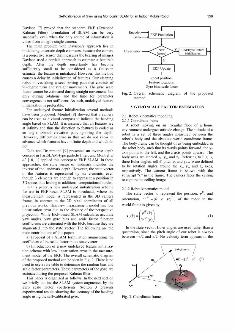
2.3.2 Measurement model of Kalman filter

Referring to Figs. 3 and 4, the observation of a feature

mi from a camera location defines a ray expressed in the

camera frame as ( ) .C C C C T

i i i ix y z=m The camera

does not directly observe ,C

im but its projection in the

image plane according to the pinhole model. In all

previous works, the measurement model of the Kalman

filter utilizes the pixel coordinates z ( )Ti i i

u v= in the

image plane, as shown in Fig. 4. The conventional

measurement model is given by

0

0

( , ) ( ),

C

i

C

ii C

i v i iC

i i

C

i

yu f

xum

v zv f

x

+

= = = = +

z h x Proj m (12)

where u0 and v0 are the camera center in pixels, and f is

the focal length. It should be noted that this model has

high linearization errors, since the perspective projection

transformation causes C

ix to be located in the

denominator. Linearization errors make the EKF

unstable when initializing uncertain depth estimates of

features, because the camera does not give any depth

information. To solve this problem, some feature

initialization methods were proposed as mentioned in the

introduction section. The concept proposed in this paper

is to regard a camera as a range and bearing sensor,

where the range information has high uncertainty. Thus,

( )C C C C T

i i i ix y z=m is used as a measurement

instead of ( ) .Ti i i

u v=z The method to calculate

( )C C C T

i i ix y z from (

iu )T

iv of the pixel coordinates

is explained in the following subsection describing

feature initialization. The proposed measurement model

is related to the estimated states via:

( ),

Ci

C C C W W bi i W i b offset

Ci

x

y C m p C p

z

= = − −

m (13)

where ,C

ix ,C

iy and C

iz are the Cartesian coordinates

of the i-th feature in the 3 dimensional camera frame (see

Figs. 3 and 4), C

WC is the transformation matrix from the

world frame to the camera frame, and pboffset is the sensor

offset from the robot center, measured in the body frame by referring to Fig. 3. Equation (13) does not suffer from linearization error caused by the perspective projection transformation. However, the new measurement model leads to another problem with conversion from 2D

information of ( )Ti i i

u v=z to 3D information of

C

im = ( ) .C C C T

i i ix y z This is explained in conjunction

with feature initialization below.

(ui,vi)

i-th feature

u

v

xc

zc

yc

ct

mC

i

1cn

2cn

Fig. 4. Image plane and camera frame.

2.3.3 Linearization error analysis EKF SLAM suffers from linearization errors. As the

linearity of the model is increased, accordingly better performance is expected from the Kalman filter. The trigonometric functions and the perspective projection are the main factors contributing to linearization errors. Equation (10) in the prediction model and (12) in the measurement model have nonlinearities due to trigonometric functions of robot orientation. When the orientation error is small, the trigonometric linearization error does not cause significant problems. A precise dead reckoning system or high update rate can be helpful to ensure that the orientation error does not become large. Furthermore, multi-map approaches [19,20] can reduce these trigonometric nonlinearities, as they maintain small orientation errors in local maps. The iterated Kalman filter framework [21] can also decrease the overall nonlinearities by applying optimization theory to EKF. Thus, we focus on reducing the linearization error due to the perspective projection. In the followings, we assume that the robot’s orientation error is negligible, and the linearization error due to the trigonometric function is not considered. This is because the conventional approaches in [9-11] also have the same error characteristics for orientation errors. Thus, the linearization error of the proposed measurement model is compared with that of the conventional measurement model.

In the conventional measurement model, the Jacobian of zi in (12) is given by

( )2

2

( , ) ( ) ( )

( , ) ( , )

0( )

| .

0( )

W C C

i i i

W C W

i i i

C

i

C C

i i C C

W WC

i

C C

i i

p m

p m p m

f y f

x x

f z f

x x

∂ ∂ ∂=

∂ ∂ ∂

⋅−

= −

⋅ −

h Proj m m

m

C C

(14)

If C

ix has a very large uncertainty, EKF SLAM will

easily fail to converge. This occurs especially when the direction of the xc–axis is close to the depth direction of a feature in early observation of features.


562

However, in the proposed measurement model, the Jacobian of the measurement model is a constant, which means there is no linearization error caused by the perspective projection.

2.3.4 Feature initialization

When an unknown feature is observed for the first time, both the feature state initial values and covariance assignment are needed. The initial location of the observed feature is defined as:

( , , ) ( ) ,W W W W b W b C Ti b offset b C im p z p C p C CΨ = + + m (15)

cos( )cos( )

sin( ) cos( ) ,

sin( )

d a e

C

i d a e

d e

h h h

h h h

h h

=

m (16)

where (hd ha he )T are the spherical coordinates of the

feature in the camera frame. hd, ha, and he are the distance, azimuth, and elevation angle to the feature in the camera frame, respectively, and are given by

( )

1

1 2 2

tan ( / ) ,

tan

d

a i i

ei i

dh

h v u

hf u v

−

−

= +

(17)

where (ui, vi) are the measured pixel coordinates and d is the assumed depth, which can be set arbitrarily. For example, d can be set as the maximum distance of the workspace. Notice that if the measurement noise covariance of hd is set to be large enough, the EKF SLAM converges even with large error between d and the true distance. This is because the proposed measurement model is perfectly linear.

The state vector and covariance are given by

xx and

,

aug

i

Taug

x z x zm

m

PP

m m m mR

=

= ∇ ∇ ∇ ∇

0I 0 I 0

0

(18)

where ∇ mx and ∇ mz are the Jacobian of the mi

function with respect to the state estimate xaug and observation z, respectively, and Rm is the measurement noise covariance matrix. To obtain Rm, the covariance of the feature in the (ct, cn1, cn2) frame (referring to Fig. 4) is introduced as follows:

2

2

0 1

2

2

0 0

0 0 ,

0 0

ct

m cn

cn

R

ε

ε

ε

=

(19)

where εct, εcn1, and εcn2 are the standard deviations of the error in the ct, cn1, and cn2 directions, respectively. ct, cn1, and cn2 are orthogonal to each other and cn1 and cn2 can be chosen in any direction.

The value of εct must be set to be large enough to

reflect the uncertainty regarding the depth. The ideal value for εct is an infinite value, but considering computational efficiency, an infinite value may not be optimal. In our system, a value over 105 cm occasionally caused problems in the process of inverting the matrix and SLAM resulted in failure. It is recommended that

43000 cm 10 cm.

ctε≤ ≤ (20)

The values given above are obtained empirically and only provide a guideline for selecting a proper value for εct.

The values of εcn1 and εcn2 approximately depend on the tracking error, calibration error, and the depth such that

2 2,

cn trk cal

d

fε ε ε≈ + (21)

where εtrk is the standard deviation of the image feature tracking error and εcal is the standard deviation of the camera calibration error.

After obtaining Rm0, Rm can be derived from

0,

C CT

m t m tR C R C= (22)

where C

tC is the rotation matrix that makes the ct-

direction parallel to the x-axis of the camera frame. The

exact form of C

tC is not expressed here for simplicity.

3. EXPERIMENTAL RESULTS

The Samsung cleaning robot VC-RE70V, which is

commercially available in the market, is used as a robot platform [13]. The onboard sensory system includes two incremental encoders that measure the rotation of each motor, and an IMU (Inertial Measurement Unit) that provides measures of the robot’s linear accelerations and angular rates. Fig. 5 shows the cleaning robot and custom-made IMU board. The IMU board has one yaw gyro (XV-3500, EPSON Corporation), one roll-pitch gyro (IDG-300, Invensense Inc.), one 3-axis accelerometer (KXPA4, Kionix Inc.), and a microprocessor. Costing less than US$20, the IMU board is affordable for cleaning robot products. The robot has one camera of 640×480 resolution that faces upward in order to capture ceiling images.

The SLAM algorithm estimates the heading angles of the robot based on the ceiling images. For feature extraction of the images, we used the Harris corner detector [14]. To track the features in the subsequent

Yaw Gyro

3-axis Accelerometer

Roll-Pitch Gyro

Fig. 5. Cleaning robot and IMU board.


563

images, we used image patches (15×15 pixels), which are able to serve as long-term landmark features with robustness to viewpoint change. To match these patches in subsequent frames, we set the search region on the image. As this region is broadened, the tracking procedure requires longer time. On the contrary, if the size of the region is reduced, tracking failure would occur more frequently. The search region was estimated based on the estimated position of the feature and the error covariance of the EKF. In the search region, we match the image patches using the Lucas-Kanade method [15].

Fig. 6 shows the ceiling image captured by the camera. The red cross marks indicate the Harris corners to be tracked, and we have chosen 5 features for computational simplicity. For application to a vacuum cleaning, the robot moves along the seed-sowing path. Thus, the robot collects a large amount of rotation data that can be used for calibration. Fig. 7 shows the feature positions estimated through the SLAM algorithm. In the figure, the 3D coordinates of the features are projected to the XY-

plane. The ellipses represent the 1σ bounds of the error covariances. Notice that the depth of the features cannot be estimated through the camera rotation alone. If the robot then moves forward, the estimated positions of the features converge to the true Cartesian coordinates.

The nominal scale factor of the yaw gyro on a specification sheet is 146.4 (deg/sec/Volt). We have examined the linearity of the scale factor of the gyro with a rate table. A custom made rate table used in our experiment consists of a direct drive motor, a PCI board, a motor controller, and an embedded computer from Yaskawa Corp and PCM-9578 from Avantech. The

available angular rate ranges from -150 to 150o/s with a resolution of 0.05o/s and accuracy of 0.06o with standard deviation of 0.0014o.

Fig. 8 shows the results obtained through this rate table. Three sample gyros were rotated at different angular velocities. Notice that the scale factor is almost the same for all of the angular velocities. We also have examined the linearity of the scale factor of other MEMS gyro products such as SMG 060 from Bosch, ADXRS 300 from Analog Devices, ENC-03 from Murata, and XV-8100 from EPSON. XV-3500 gyroscope shows the best linearity performance compared to the other products. The scale factor can be considered as a linear function for XV-3500, which means that the error of the scale factor, δωz, in (7) is modeled with a first order function. To model the bias Bz in (8) of the yaw gyro, its output was recorded over a long period of time when subjected to zero input. The results are shown in Fig. 9. Using the least square fit method, the parameters of (8) are given as C1 = 0.6, C2 = 6.04 and T = 500.

Fig. 10 shows the convergence of the estimated parameter a1 in (7). It converges to the true value of 135.5, which was obtained using the rate table.

After getting calibrated gyro parameters by performing EKF SLAM, the performance of heading angle estimation between the calibrated and uncalibrated

Fig. 6. Captured ceiling image.

-20 -15 -10 -5 0 5 10 15-10

-5

0

5

10

15

20

25

x (m)

y(m

)

Fig. 7. Estimated feature positions.

20 30 40 50 60 70 80 90135.3

135.35

135.4

135.45

135.5

135.55

135.6

135.65

135.7

Angular velocity (deg/sec)

Scale factor (deg/sec/Volt)

sample #1

sample #2

sample #3

Fig. 8. Scale factors measured at different angular velocities using a rate table.

0 500 1000 1500 2000 25000

1

2

3

4

5

6

7

8

Measured output

Modelled output

Time[sec]

ωz

[deg/sec]

Fig. 9. Output of the yaw gyro when subjected to zero input.


564

gyros was compared in Table 1. Note that the camera was not used in this case in order to clearly see the sole performance of gyro calibration. Table 1 shows the heading angle errors for both cases after 10 clockwise rotations. The mean value of the absolute error is reduced to 0.4% of the original error with the calibrated gyro. Fig. 11 shows the angle errors after the robot finished 10 minutes of cleaning. We tested 4 samples and repeated 3 experiments for each sample. The mean and standard deviation of the angle error for the calibrated gyro are -0.18o and 0.91o and the uncalibrated gyro with the nominal scale factor shows considerable part-to-part

variation in the angle error. It should be noted that the scale factor calibration reduces the angle error dramatically. Even though the gyro used in this work is a low-lost MEMS gyro, it shows quite good performance after scale factor calibration. Fig. 12 shows the improvement of the position accuracy of dead reckoning. The robot started from the (0, 0) position marked with a circle and stopped at the position marked as ‘x’. The position error of the calibrated gyro at the final position is 13.8 cm and that of the uncalibrated gyro is 66.0 cm. Ground truth data are obtained by a Hawk digital motion tracker system produced by Motion Analysis Inc., which has accuracy within 5mm. We can see that the heading angle improvement provides more accurate position estimation.

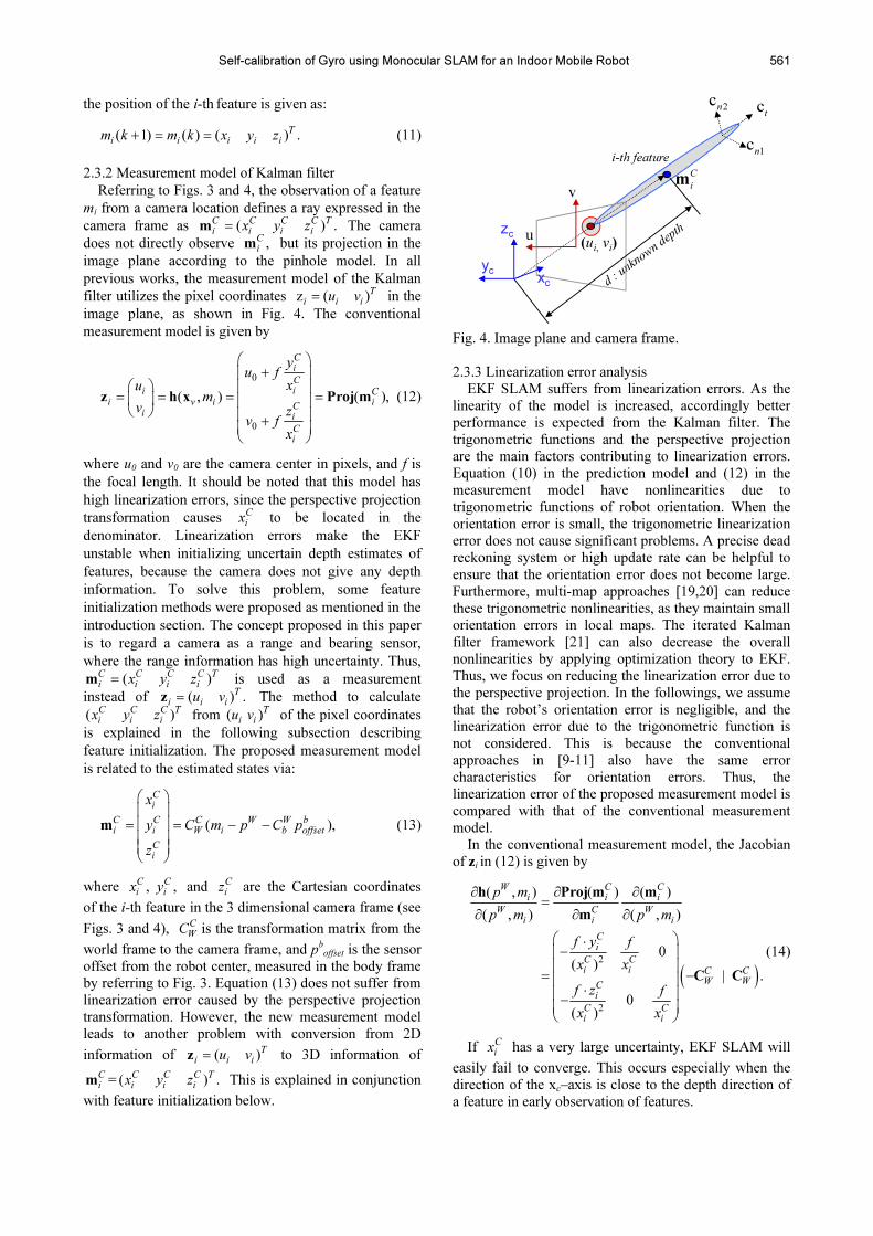
We have performed an additional experiment to show the performance of SLAM with a calibrated gyro. In Fig. 13, the robot started from (0, 0) position and stopped at position indicated by a circle. The solid line indicates the ground truth data obtained by the motion tracker system, the dashed line denotes the dead-reckoning localization result with a calibrated gyro without SLAM, and the x-marked line indicates the localization result with SLAM with a calibrated gyro. It is clear that the SLAM can give an accurate localization result compared to the dead-reckoning system.

Table 1. The heading angle error after 10 rotations (unit:deg).

With Nominal

Scale Factor

With Calibrated

Scale Factor

1 24.73 -0.17

2 23.33 -1.57

3 23.70 -1.20

4 23.61 -1.29

5 24.23 -0.68

6 -25.92 0.59

7 -25.78 0.76

8 -25.81 0.74

9 -25.34 1.17

10 -25.63 0.91

Mean Absolute Error 24.83 0.99

-50 0 50 100 150 200 250 300 350 400 450-50

0

50

100

150

200

250

300

x (cm)

y (cm)

ground truth

calibrated

uncalibrated

Fig. 12. Trajectory plots of the calibrated gyro and the uncalibrated gyro.

0 2 4 6 8 10 12 14 16 18 200

50

100

150

time (sec)

a1

(deg/sec/Volt)

True value

0 2 4 6 8 10 12 14 16 18 200

50

100

150

time (sec)

a1

(deg/sec/Volt)

True value

Fig. 10. Convergence of the scale factor parameter.

-10 -8 -6 -4 -2 0 2 4 6 8 100

0.5

1

1.5

2

2.5

3

3.5

4

Angle error (deg)

num

ber

of

occurr

ence

(a) With calibrated scale factor.

-10 -8 -6 -4 -2 0 2 4 6 8 100

0.5

1

1.5

2

2.5

3

3.5

4

4.5

5

Angle error (deg)

nu

mb

er

of

occu

rren

ce

(b) With nominal scale factor.

Fig. 11. Histogram of angle errors after 10 minutes ofcleaning operation.


565

Fig. 13. Trajectory plots of the dead-reckoning and SLAM results with a calibrated gyro.

0 10 20 30 40 500

50

100

150

200

250

robot movement (cm)

error of feautre location (cm)

conventional method

inverse depth method

proposed method

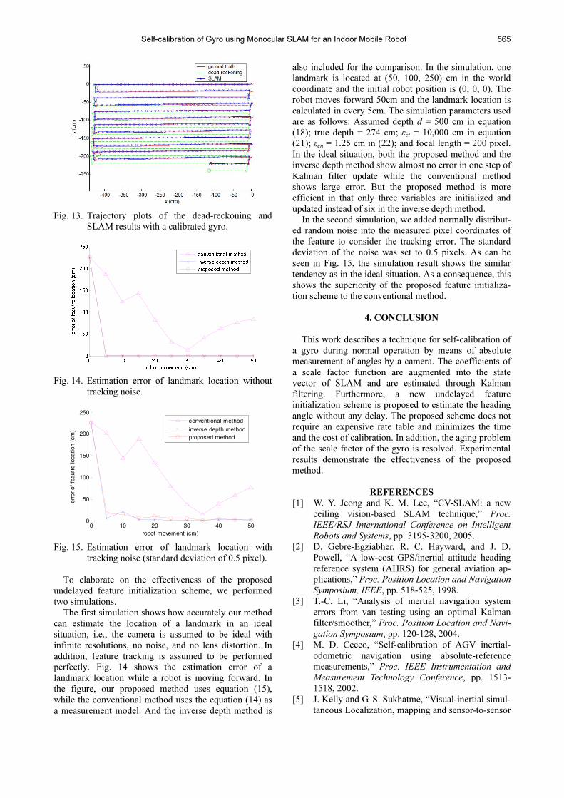
Fig. 14. Estimation error of landmark location without tracking noise.

0 10 20 30 40 500

50

100

150

200

250

robot movement (cm)

error of feautre lo

catio

n (cm

)

conventional method

inverse depth method

proposed method

Fig. 15. Estimation error of landmark location with tracking noise (standard deviation of 0.5 pixel).

To elaborate on the effectiveness of the proposed

undelayed feature initialization scheme, we performed two simulations.

The first simulation shows how accurately our method can estimate the location of a landmark in an ideal situation, i.e., the camera is assumed to be ideal with infinite resolutions, no noise, and no lens distortion. In addition, feature tracking is assumed to be performed perfectly. Fig. 14 shows the estimation error of a landmark location while a robot is moving forward. In the figure, our proposed method uses equation (15), while the conventional method uses the equation (14) as a measurement model. And the inverse depth method is

also included for the comparison. In the simulation, one landmark is located at (50, 100, 250) cm in the world coordinate and the initial robot position is (0, 0, 0). The robot moves forward 50cm and the landmark location is calculated in every 5cm. The simulation parameters used are as follows: Assumed depth d = 500 cm in equation (18); true depth = 274 cm; εct = 10,000 cm in equation (21); εcn = 1.25 cm in (22); and focal length = 200 pixel. In the ideal situation, both the proposed method and the inverse depth method show almost no error in one step of Kalman filter update while the conventional method shows large error. But the proposed method is more efficient in that only three variables are initialized and updated instead of six in the inverse depth method.

In the second simulation, we added normally distribut-ed random noise into the measured pixel coordinates of the feature to consider the tracking error. The standard deviation of the noise was set to 0.5 pixels. As can be seen in Fig. 15, the simulation result shows the similar tendency as in the ideal situation. As a consequence, this shows the superiority of the proposed feature initializa-tion scheme to the conventional method.

4. CONCLUSION

This work describes a technique for self-calibration of

a gyro during normal operation by means of absolute measurement of angles by a camera. The coefficients of a scale factor function are augmented into the state vector of SLAM and are estimated through Kalman filtering. Furthermore, a new undelayed feature initialization scheme is proposed to estimate the heading angle without any delay. The proposed scheme does not require an expensive rate table and minimizes the time and the cost of calibration. In addition, the aging problem of the scale factor of the gyro is resolved. Experimental results demonstrate the effectiveness of the proposed method.

REFERENCES

[1] W. Y. Jeong and K. M. Lee, “CV-SLAM: a new ceiling vision-based SLAM technique,” Proc.

IEEE/RSJ International Conference on Intelligent

Robots and Systems, pp. 3195-3200, 2005. [2] D. Gebre-Egziabher, R. C. Hayward, and J. D.

Powell, “A low-cost GPS/inertial attitude heading reference system (AHRS) for general aviation ap-plications,” Proc. Position Location and Navigation

Symposium, IEEE, pp. 518-525, 1998. [3] T.-C. Li, “Analysis of inertial navigation system

errors from van testing using an optimal Kalman filter/smoother,” Proc. Position Location and Navi-

gation Symposium, pp. 120-128, 2004. [4] M. D. Cecco, “Self-calibration of AGV inertial-

odometric navigation using absolute-reference measurements,” Proc. IEEE Instrumentation and

Measurement Technology Conference, pp. 1513-1518, 2002.

[5] J. Kelly and G. S. Sukhatme, “Visual-inertial simul-taneous Localization, mapping and sensor-to-sensor


566

self-calibration,” Proc. IEEE Int'l Symp. Computa-tional Intelligence in Robotics and Automation, Daejeon, Korea, Dec. 2009.

[6] J. Lobo and J. Dias, “Relative pose calibration be-tween visual and inertial sensors,” Int’l J. Robotics Research, vol. 26, no. 6, pp. 561-575, June 2007.

[7] A. J. Davison, “Real-time simultaneous localization and mapping with a single camera,” Proc. Interna-tional Conference on Computer Vision, 2003.

[8] J. M. M. Montiel and A. J. Davison, “A visual compass based on SLAM,” Proc. IEEE Interna-tional Conference on Robotics and Automation, pp. 1917-1922, 2006.

[9] E. Eade and T. Drummond, “Scalable monocular SLAM,” Proc. IEEE Conference on Computer Vi-sion and Pattern Recognition, 2006.

[10] J. M. M. Montiel, J. Civera, and A. J. Davison, “Unified inverse depth parameterization for mo-nocular SLAM,” Proc. Robotics: Science and Sys-tems, Philadelphia, USA, 2006.

[11] J. Civera, A. J. Davison, and J. M. M. Montiel, “In-verse depth to depth conversion for monocular SLAM,” Proc. IEEE International Conference on Robotics and Automation (ICRA), Roma, Italy, 2007.

[12] H. Chung, L. Ojeda, and J. Borenstein, “Sensor fusion for mobile robot dead-reckoning with a pre-cision-calibrated fiber optic gyroscope,” Proc. IEEE International Conference on Robotics and Automation, pp. 3588-3593, 2001.

[13] H. Myung, H.-K. Lee, K. Choi, and S. Bang, “Mo-bile robot Localization with gyroscope and con-strained Kalman filter,” International Journal of Control, Automation, and Systems, vol. 8, no. 3, pp. 667-676, June 2010.

[14] C. Harris and M. Stephens, “A combined corner and edge detector,” Proc. of the 4th Alvey Vision Conference, pp. 147-151, 1988.

[15] S. Baker and I. Mattews, “Lucas-Kanade 20 years on: a unifying framework Part 1,” International Journal of Computer Vision, vol. 56, no. 3, pp. 221-225, 2004.

[16] B. Barshan and H. F. Durrant-Whyte, “Inertial navigation systems for mobile robots,” IEEE Trans. on Robotics and Automation, vol. 11, no. 3, pp. 328-342, 1995.

[17] S. I. Roumeliotis, G. S. Sukhatme, and G. A. Bekey, “Circumventing dynamic modeling: evaluation of the error-state Kalman filter applied to mobile robot Localization,” Proc. IEEE International Confer-ence on Robotics and Automation, pp. 1656-1663, 1999.

[18] D. H. Titterson and J. L. Weston, Chapter 4 of Strapdown Inertial Navigation Technology, 2nd Edition, The Institution of Electrical Engineers, 2004.

[19] J. D. Tardós, J. Neira, P. M. Newman, and J. J. Leonard, “Robust mapping and localization in in-door environments using Sonar data,” Int’l Journal of Robotics Research, vol. 21, no. 4, pp. 311-330,

2002. [20] L. M. Paz, J. D. Tardós, and J. Neira, “Divide and

Conquer: EKF SLAM in O(n),” IEEE Trans. on Robotics, vol. 24, no. 5, pp. 1107-1120, October 2008.

[21] S. Tully, H. Moon, G. Kantor, and H. Choset, “Iter-ated filters for bearing-only SLAM,” Proc. IEEE International Conference on Robotics and Automa-tion, May 2008.

Hyoung-Ki Lee received his Ph.D. de-gree in robotics from KAIST (Korea Advanced Institute of Science and Tech-nology), Daejeon, Korea in 1998. In 1999, he worked as a Postdoctoral Fellow in Mechanical Engineering Lab., AIST, in Japan. In 2000, he joined Samsung Ad-vanced Institute of Technology and is developing a vacuum cleaning robot with

a localization function as a part of a home service robot project. His research interests include SLAM (Simultaneous Localiza-tion And Mapping) for home robots, fusing different kinds of sensors (inertial sensors, cameras, range finders, etc.), and de-veloping new low-cost sensor modules such as a MEMS gyro sensor module and structured light range finder.

Kiwan Choi received his M.S. degree in mechanical design and production engi-neering from Seoul National University, Korea in 1999. He is currently a senior researcher in the Robot Navigation Group, Samsung Advanced Institute of Technology, Samsung Electronics Co., Ltd. His current research interests in-clude SLAM (Simultaneous Localization

And Mapping), inertial navigation systems, and mobile robotics.

Jiyoung Park received her M.S. degree in electronics and electrical engineering from KAIST in 2006. She is currently a senior researcher with the Robot Naviga-tion Group, Advanced Institute of Tech-nology, Samsung Electronics Inc. Her current research interests include inertial navigation systems and mobile robotics.

Hyun Myung received his Ph.D. degree in electrical engineering from KAIST (Korea Advanced Institute of Science and Technology), Daejeon, Korea in 1998. He is currently an assistant professor in the Dept. of Civil and Environmental Engi-neering, and also an adjunct professor of the Robotics Program and KIUSS (KAIST Institute for Urban Space and

Systems) at KAIST. He was a principal researcher in SAIT (Samsung Advanced Institute of Technology, Samsung Elec-tronics Co., Ltd.), Yongin, Korea (2003.7-2008.2). He was a director in Emersys Corp. (2002.3-2003.6) and a senior re-searcher in ETRI (Electronics and Telecommunications Re-search Institute) (1998.9-2002.2), Korea. His research interests are in the areas of mobile robot navigation, SLAM (Simultane-ous Localization and Mapping), evolutionary computation, numerical and combinatorial optimization, and intelligent con-trol based on soft computing techniques.

Documents

Self-calibration of gyro using monocular SLAM for an indoor mobile robot