Self-Adaptive Generator Protection - GE Grid Solutions · Self-Adaptive Generator Protection Methods ... used to derive a differential and restraint signal. The relay has a percent

60th

Annual Georgia Tech Protective Relaying Conference

1

I. INTRODUCTION

The setting of many of the functions that are used to

protect synchronous generators is relatively

straightforward, requiring system or machine data that is

readily available to the protection engineer. However,

there are occasions where the effective application of a

protection function requires detailed measurement and

analysis of operational data from the machine. This

paper identifies two such functions: Split Phase

protection and 3rd

Harmonic Neutral Undervoltage

protection and discusses the particular application issues

associated with each. These functions are responsible

for detection of two of the most common types of stator

winding failures; inter-turn faults and ground faults. A

new algorithm is presented that can respond to the

influencing system conditions and automatically adapt

these functions accordingly. The resulting protection

schemes are more sensitive, less likely to mis-operate,

and are easier to set than their conventional

counterparts.

II. INTERTURN FAULTS

A hydroelectric generator is often wound with a double-

layer, multi-turn winding. The winding may be a single

circuit or there may be two, four, six or eight branches

in parallel. Under normal operation there is very little

difference in the current in each branch. However,

during an internal fault, currents will circulate between

the parallel branches of the winding within one phase.

Split phase protection takes advantage of this

characteristic by measuring the current unbalance

between these parallel branches. In hydro machines a

significant percentage of stator faults begin as turn-to-

turn faults [1]. Due to the very high effective turns-ratio

between the windings and the shorted turn, inter-turn

faults cause extremely high currents in the faulted loop

leading to quickly progressing damage.

These faults are not detectable by the stator differential

or ground fault protections since there is no difference

between the currents at the output and the neutral

terminals and there is no path for fault current to ground.

If these faults can be detected before they evolve in to

phase or ground faults then the damage to the machine

and associated downtime can be greatly reduced.

Therefore the split phase protection should ideally be

sensitive enough to operate for a single-turn fault in the

winding of the machine.

A. Detection Methods

There are several methods currently in use today.

1) Scheme A

In scheme A, a neutral point is brought out for each

parallel circuit. An overcurrent element is connected

between each neutral. During an inter-turn fault, a

circulating current is produced in the faulted phase that

is passed between the neutrals.

R

Figure 1 −−−− Scheme A

Self-Adaptive Generator Protection Methods

D. Finney, B. Kasztenny, M. McClure, G. Brunello – General Electric

A. LaCroix – Hydro Québec

60th


2

2) Scheme B

In this scheme a differential and restraint signal are

derived using currents from both sides of the machine.

One current represents the total current in the machine

while the other is the current from a CT representing 1/2

the total current. This scheme is also known as

“combined split phase and differential” or “partial

longitudinal differential”.

R

Figure 2 −−−− Scheme B

3) Scheme C

In scheme C, the currents from each parallel circuit are

used to derive a differential and restraint signal. The

relay has a percent slope characteristic. The restraint

signal provides security against a false differential

produced during an external fault while still allowing

fast operation during internal faults. This scheme is

sometimes known as “transverse differential”.

R

Figure 3 −−−− Scheme C

4) Scheme D

The scheme shown in Figure 4 also responds to the

difference between the currents in the two circuits.

However, the summation is done outside the relay.

Therefore this method cannot derive a restraint signal.

An instantaneous element using this signal must be set

high enough to avoid pickup during an external fault.

This will make the element relatively ineffective for

detection of single-turn faults. As such this scheme

usually employs a definite time or inverse time

characteristic for security.

R

Figure 4 −−−− Scheme D

5) Scheme E

In this scheme a window-type CT is used to measure the

difference between the current in each circuit, as shown

in Figure 5. This method avoids the CT error issues of

Scheme D.

R

Figure 5 −−−− Scheme E

B. Characterization

Under normal operation the level of the inherent split

phase current is usually less then 0.5% of the rated

machine current [1]. During an external fault many

machines produce a transient circulating current. The

magnitude of this transient can be several times larger

than the steady state current and may persist for upwards

60th


3

of 30 cycles [1]. For an internal fault, the magnitude of

the circulating current corresponding to a single-turn

short is dependent on several factors. These include the

type of the winding (adjacent versus alternate pole) and

the number of poles.

C. Application

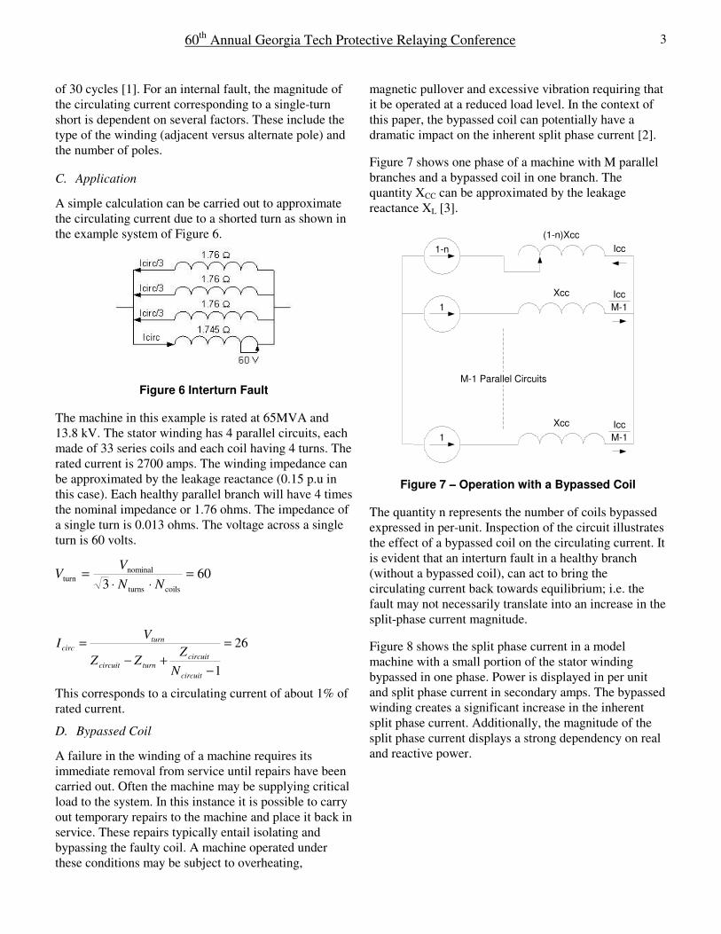
A simple calculation can be carried out to approximate

the circulating current due to a shorted turn as shown in

the example system of Figure 6.

Figure 6 Interturn Fault

The machine in this example is rated at 65MVA and

13.8 kV. The stator winding has 4 parallel circuits, each

made of 33 series coils and each coil having 4 turns. The

rated current is 2700 amps. The winding impedance can

be approximated by the leakage reactance (0.15 p.u in

this case). Each healthy parallel branch will have 4 times

the nominal impedance or 1.76 ohms. The impedance of

a single turn is 0.013 ohms. The voltage across a single

turn is 60 volts.

603 coilsturns

nominalturn =

⋅⋅=

NN

VV

26

1

=

−+−

=

circuit

circuitturncircuit

turncirc

N

ZZZ

VI

This corresponds to a circulating current of about 1% of

rated current.

D. Bypassed Coil

A failure in the winding of a machine requires its

immediate removal from service until repairs have been

carried out. Often the machine may be supplying critical

load to the system. In this instance it is possible to carry

out temporary repairs to the machine and place it back in

service. These repairs typically entail isolating and

bypassing the faulty coil. A machine operated under

these conditions may be subject to overheating,

magnetic pullover and excessive vibration requiring that

it be operated at a reduced load level. In the context of

this paper, the bypassed coil can potentially have a

dramatic impact on the inherent split phase current [2].

Figure 7 shows one phase of a machine with M parallel

branches and a bypassed coil in one branch. The

quantity XCC can be approximated by the leakage

reactance XL [3].

M-1 Parallel Circuits

Icc

Icc

M-1

Icc

M-1

(1-n)Xcc

Xcc

Xcc

1-n

1

1

Figure 7 −−−− Operation with a Bypassed Coil

The quantity n represents the number of coils bypassed

expressed in per-unit. Inspection of the circuit illustrates

the effect of a bypassed coil on the circulating current. It

is evident that an interturn fault in a healthy branch

(without a bypassed coil), can act to bring the

circulating current back towards equilibrium; i.e. the

fault may not necessarily translate into an increase in the

split-phase current magnitude.

Figure 8 shows the split phase current in a model

machine with a small portion of the stator winding

bypassed in one phase. Power is displayed in per unit

and split phase current in secondary amps. The bypassed

winding creates a significant increase in the inherent

split phase current. Additionally, the magnitude of the

split phase current displays a strong dependency on real

and reactive power.

60th


4

Figure 8 −−−− Split Phase Current Measurements

As a result the pickup setting of the split phase

protection must be increased to prevent false operation.

This can make the function ineffective for the detection

of single-turn faults.

III. STATOR GROUND FAULTS

Stator ground faults are short circuits between any of the

stator windings and ground, via the iron core of the

stator. Typically, when a single machine is connected to

the power system through a step-up transformer, it is

grounded through high impedance. As a result, the

amount of the short circuit current during stator ground

faults is driven by the amount of capacitive coupling in

the machine and its step-up transformer. Therefore when

a ground fault occurs, very small capacitive current

flows making the short circuit difficult to detect.

Ground faults can be detected throughout most of the

winding through the use of an overvoltage relay

responding to the fundamental component of the voltage

across the grounding impedance. The magnitude of this

voltage is proportional to the location of the fault.

Therefore, for faults at or near the neutral of the

machine, this element is ineffective [4].

Little or no damage is done to the machine as a result of

a ground fault close to the neutral. It does, however,

prevent the overvoltage protection from detecting a

second ground fault. If a second ground fault occurs, the

grounding impedance does not limit the fault current. If

the second ground is on the same phase it will not be

detectable by the differential. The result can be

potentially catastrophic damage to the machine [5].

Therefore, a second method to detect faults close to the

neutral and effectively prevent widespread damage to

the machine is beneficial. This second method is

sometimes known as 100% stator ground fault

protection.

A. Methods for Detection

Several techniques for 100% stator ground fault

detection take advantage of the third harmonic voltage

generated by the machine itself [5].

V3

V3

V3

V3N V

3T

k

Figure 9 Stator Ground Fault

Under normal operating conditions a portion of the 3rd

harmonic appears across the generator terminals and a

portion appears across the grounding impedance as

shown by the green line in Figure 10. For a fault at k, the

distribution of the third shifts to the red line. This causes

the third harmonic at the neutral to decrease and the

third harmonic at the terminals to increase.

Thir

d H

arm

onic

Volta

ge

∆V

3N

100%0% % of Stator Winding

k

Figure 10 Third Harmonic Distribution

If the third harmonic can be measured both at the

generator neutral and at the terminals, then a differential

scheme can be applied [5]. This scheme is less sensitive

to variations in the third harmonic due to machine

loading. However, if the VT connection does not permit

measurement of the third harmonic at the generator

terminal end [5], comparison of the neutral and terminal

end third harmonic signatures is impossible, and then

only the third harmonic neutral undervoltage element

may be applied.

60th


5

Figure 11 – Neutral Undervoltage Scheme

The third harmonic undervoltage element uses the

voltage that forms across the high impedance ground,

which is connected to the neutral point of the generator

unless a better path to ground is presented. Figure 12 is

an example of the third harmonic voltage measured at

the neutral of a generator at various levels of real and

reactive loading. Power is displayed in primary units and

third harmonic voltage is displayed in secondary volts.

During a ground fault close to the generator neutral the

third harmonic voltage will decrease or drop to zero.

Figure 12 −−−− Third Harmonic Voltage Characteristic

In the scheme of Figure 11 a neutral voltage is measured

from the machine neutral point. During a stator ground

fault, the third harmonic will flow into the ground fault,

shunting the neutral grounding path, and the

measurement of neutral voltage will drop to or near

zero.

B. Characterization

The characteristic of the third harmonic varies

considerably between different machine designs; it can

also vary considerably between machines of the same

design due to manufacturing variation. Under normal

operation the level of the third harmonic neutral voltage

can vary considerably based upon machine output

(MW), power factor (PF) and machine voltage (kV).

In order to provide optimum protection for the machine,

the complete third harmonic characteristic must be

found and the setting should be calculated based on this

data. Data must be collected and then plotted with

output (MW) along the X-axis and third harmonic

neutral voltage (V) along the Y-axis as shown in Figure

13.

Once this data is plotted an appropriate tripping voltage

should be determined. It should be significantly high

such that the protection will function, even when the

fault is farther up on the winding. The setting must also

allow enough margin to allow for variation and errors in

the data collection and input accuracy.

A power blocking value should be derived so that it

complements the tripping voltage. The local minimums

in the third harmonic characteristic should be blocked

allowing the highest possible tripping voltage.

There are several options for setting this function.

1) Type Testing

A simple method of setting this function utilizes the data

from type tests for machines of the same design.

Electrical machines of the same design and manufacture

can be type tested and a standard set point can be

calculated and used. This provides the easiest solution

however it is the least effective and can provide less

protection or lead to nuisance tripping.

2) Site Testing

The setting can be derived by taking site data for each

machine by running the machine through the range of

power output and power factor. Taking data at regular

intervals will allow for a sufficiently accurate setting to

allow for protection while keeping from false tripping.

This method is provides good protection but is more

expensive than type tests and still allows the opportunity

for data collection errors. An example of the data

collected during a site test is shown in Figure 13.

60th


6

Figure 13 – Third Harmonic Neutral Voltage Data

C. Electronic Data Collection

If a data logger with sufficient memory exists in the

applied protective relay [7], data logging can be used to

collect operating data over the operating time. This data

can be extracted from the data logger and used to

calculate the setting. This method provides much more

accurate characterization of the third harmonic, however

the data may not cover the entire operating region. If the

machine has not operated in those regions the protection

setting decision may be made with incomplete data,

which could lead to nuisance tripping or insufficient

protection.

IV. SELF-ADAPTIVE PROTECTION PRINCIPLES

The previous sections describe the deviation that can

sometimes occur in the operating signals of the split

phase and 3rd

harmonic undervoltage element as a result

of active and reactive loading of the machine and the

resulting problems relating to setting selection. It is

proposed that for both functions a method could be

derived to automatically adapt to these variables.

The method would measure and log the variations in the

operating quantity over time in order to learn the

characteristics under various loading conditions and

operate based on a departure from this characteristic in

order to protect the machine.

Implemented in a microprocessor-based device, data

collection would entail sampling the voltages and

currents and the operating quantities, filtering digitally,

extracting magnitudes/angles using a standard Fourier

algorithm, and calculating active and reactive quantities

from these.

The method would allow for the protection to become

active as soon as the data has been collected. The

function could be proactively enabled and disabled to

protect for operating conditions where sufficient

operation data has been collected and block for

operating conditions where insufficient data has been

collected.

The function would require a security margin to account

for measurement errors.

A best-fit curve could be calculated to approximate the

operating characteristic; there are several methods for

forming this function. This method would require

recalculation of the curve each time data is collected and

would be very processor intensive.

Alternately, the operating characteristic could be

approximated by an array of data points stored to create

a mesh of operating signal values spaced equally over

the active-reactive power region. This method requires

more memory to store the data but is less processor-

intensive.

Data would be collected whenever the machine is in

operation. The data would be used to update the array

holding the operating data for the machine. Since the

array consists of a finite number of elements, the

measured value of the operating signal data would not

usually correspond exactly to a point in the array (points

I-IV in Figure 14).

MW

MVAR

III

IVIII

Measured

data

Figure 14 - Operating Data Array

Therefore either the point closest to the measured value

could be updated or all four adjacent points could be

updated simultaneously.

Before the data could be used for fault detection the data

must be validated. This could be a manual operation –

the data could be downloaded and analyzed. If

satisfactory the function could then be placed in-service.

60th


7

Alternately, the validation of the data could be

automated. In such a scheme, a test could be carried out

on the data to determine whether or not it is changing

dramatically between successive samples. An additional

test would be to examine the smoothness of the

characteristic over successive data points.

An important consideration is the number of points in

the array required for an accurate representation of the

data. The factors influencing this determination include

the smoothness of the operating characteristic, the

method used to interpolate between points in the array

and the accuracy required by the function.

Once the data has been validated it may be used for fault

detection. Again, it is unlikely that the measured value

of P and Q will correspond to a point in the array.

An expected operating value must therefore be

calculated for each value of P and Q. Since this

function is adaptive the value must be calculated in real

time.

Terminal voltage can have a significant effect on the

quiescent value of the operating signal. The signal can

be similarly affected during other system disturbances.

Therefore it is important to inhibit learning during these

periods. This can be achieved by monitoring of the

positive sequence voltage and current. Learning is

inhibited if the positive sequence voltage is lower than

its nominal range. Learning is also inhibited when the

positive sequence current is greater than its nominal

value. Additionally, some machines may exhibit a

significant difference in the operating signal between the

offline and online state. In such cases, learning may also

be supervised by breaker position. Once system

conditions return to normal for a definite period, normal

learning can resume. Similar supervision can be applied

in the tripping mode.

V. DEVELOPMENT OF ADAPTIVE ALGORITHMS

As explained in the previous section adaptive algorithms

in this application consist of two parts. First, a learning

procedure is required to establish the operate/restraint

surface based on the measured data over longer periods

of time. Second, an operate logic is required to use the

learned surface for tripping at a given time.

This section presents practical ways of implementing

such algorithm. The equations are derived for two-

dimensional situations, i.e. when a single operating

quantity depends on two variables, but can be easily

extended onto generalized multi-dimensional cases.

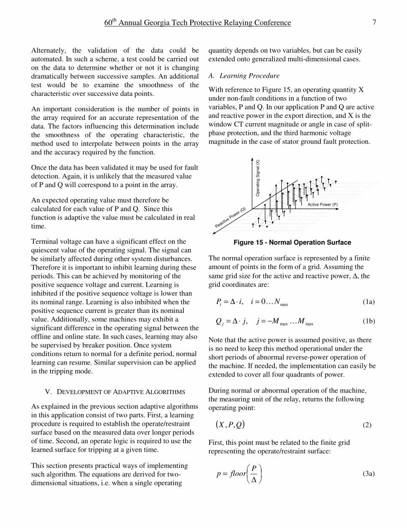
A. Learning Procedure

With reference to Figure 15, an operating quantity X

under non-fault conditions in a function of two

variables, P and Q. In our application P and Q are active

and reactive power in the export direction, and X is the

window CT current magnitude or angle in case of split-

phase protection, and the third harmonic voltage

magnitude in the case of stator ground fault protection.

Reactive P

ower (Q)

Opera

ting

Sig

nal (X

)

Active Power (P)

Figure 15 - Normal Operation Surface

The normal operation surface is represented by a finite

amount of points in the form of a grid. Assuming the

same grid size for the active and reactive power, ∆, the

grid coordinates are:

max0, NiiPi …=⋅∆= (1a)

maxmax, MMjjQ j …−=⋅∆= (1b)

Note that the active power is assumed positive, as there

is no need to keep this method operational under the

short periods of abnormal reverse-power operation of

the machine. If needed, the implementation can easily be

extended to cover all four quadrants of power.

During normal or abnormal operation of the machine,

the measuring unit of the relay, returns the following

operating point:

( )QPX ,, (2)

First, this point must be related to the finite grid

representing the operate/restraint surface:

∆=

Pfloorp (3a)

60th


8

∆=

Qfloorq (3b)

Where floor stands for rounding down to the nearest

integer.

The operating point is located between the following

four corners of the grid (Figure 16):

( ) ( ) ( ) ( )qpqpqpqp ,1,1,1,1,,, ++++ (4)

During the learning phase, the value of X shall be used

to adjust all four corners surrounding the operating

point. Different approaches can be used.

In one method, all four points are treated equally and

use the same value to adjust the value of the learned X.

For example:

( ) XXX OLDqpNEWqp ⋅+⋅−= αα ),(),( 1 (5a)

In the above, a smoothing filter is used for extra

security. Only a small fraction of the measurement (α) is

added to the previous value. In this way the sought value

at the (p, q) point of the grid reaches its steady state

asymptotically, and the value of α controls the speed of

learning. The higher the α, the faster will be the

convergence.

Similar equations are used to adjust the other three

corners around the measuring point:

( ) XXX OLDqpNEWqp ⋅+⋅−= ++ αα )1,()1,( 1 (5b)

( ) XXX OLDqpNEWqp ⋅+⋅−= ++++ αα )1,1()1,1( 1 (5c)

( ) XXX OLDqpNEWqp ⋅+⋅−= ++ αα ),1(),1( 1 (5d)

In another method, the closer the operating point to a

given point of the grid, the higher the impact on the

learned value for that point of the grid. This can be

accomplished using the following equations for

learning.

First, the relative distances between the operating point

and the four corners are calculated:

( ) ( )2

22

),(2 ∆⋅

−∆⋅+−∆⋅=

QqPpD qp (6a)

( ) ( )2

22

)1,(2 ∆⋅

−∆+∆⋅+−∆⋅=+

QqPpD qp (6b)

( ) ( )2

22

)1,1(2 ∆⋅

−∆+∆⋅+−∆+∆⋅=++

QqPpD qp (6c)

( ) ( )2

22

),1(2 ∆⋅

−∆⋅+−∆+∆⋅=+

QqPpD qp (6d)

These distances can be used to speed up the learning for

corners located closer to the operating point:

( )( )( ) XD

XDX

qp

OLDqpqpNEWqp

⋅−⋅+

⋅−⋅−=

),(

),(),(),(

1

11

α

α (7a)

( )( )( ) XD

XDX

qp

OLDqpqpNEWqp

⋅−⋅+

⋅−⋅−=

+

+++

)1,(

)1,()1,()1,(

1

11

α

α (7b)

( )( )( ) XD

XDX

qp

OLDqpqpNEWqp

⋅−⋅+

⋅−⋅−=

++

++++++

)1,1(

)1,1()1,1()1,1(

1

11

α

α(7c)

( )( )( ) XD

XDX

qp

OLDqpqpNEWqp

⋅−⋅+

⋅−⋅−=

+

+++

),1(

),1(),1(),1(

1

11

α

α (7d)

Version (7) has an advantage over version (5) when the

operating point lingers at the border line between two

different segments of the grid – it provides smooth

transition between training one set of point versus a

different set of points on the grid.

60th


9

Active Power (P)

Reactive

Pow

er

(Q)

(p+1,q)(p,q)

(p+1,q+1)(p,q+1)

(P,Q)

D(p,q+1)

D(p,q)

D(p+1,q)

D(p+1,q+1)

Figure 16 - Calculation of Distances

Equations (5) and (7) average the data when forming the

operate/restraint surface by means of exponential

convergence. A separate check must be designed to

decide if a given value learned in the process is final and

could be trusted, i.e. used by the operating logic.

Two criteria are used to decide if a given point is

properly trained.

First, it is checked if the update process as dictated by

equation (5) or (7) stops changing the value. This is

determined by checking the increment after the update

takes place. For example, when using form (7) one

checks:

NEWqpOLDqpNEWqpqp XXXFLG ),(),(),(),(1 ⋅<−= β (8)

Where β is an arbitrary value expressing the percentage

difference that identifies the steady state is being

reached.

The above flag is calculated each time a given point on

the grid is updated as a part of the learning procedure

that is for all four points surrounding the operating

point.

Second, it is checked with the surface emerging in

response to learning is smooth. This is determined by

checking differences between the surrounding points on

the grid:

…&),(),1(),(),(2 qpqpqpqp XXXFLG ⋅<−= − δ

…… && ),(),1(),( qpqpqp XXX ⋅<− + δ

…… && ),()1,(),( qpqpqp XXX ⋅<− − δ

),()1,(),(& qpqpqp XXX ⋅<− + δ… (9)

Where δ is an arbitrary factor. Equation (9) takes

exception for the points on the outer border of the grid –

these points have only three, not four, neighboring

points.

For a given point on the grid (p, q) to be considered

trained, both the flags (8) and (9) must be asserted.

The learning procedure can be summarized as follows:

1. Take the measurement of the operating point

(equation (2)).

2. Calculate the coordinates of the grid (equation

(3)).

3. Update the four corners of the grid surrounding

the operating point (equations (6) and (7)).

4. Calculate the first validity flag for the four

updated points (equation (8)).

5. Calculate the second validity flag for the four

updated points and their neighbors (equation (9)).

6. Update the validity flags for the affected points on

the grid.

VI. SIMULATION RESULTS

Figures 17-21, illustrate the learning procedure using an

arbitrary surface. In this example the operating quantity

is given by the following equation:

22QP

ePX+⋅= (10)

For the third harmonic undervoltage function the

following design constants are selected:

25,25,05.0 maxmax ===∆ MNpu

60th


10

03.0,03.0,05.0 === δβα .

For the split phase function the following design

constants are selected for both the current magnitude

and angle:

10,10,125.0 maxmax ===∆ MNpu

03.0,03.0,05.0 === δβα .

The above means the (P, Q) grid stretches as follows

(0,1.25pu) for the active, and the reactive power.

Figure 17 presents function (10). This is the target

function that should be learned by the procedure.

Figure 17 - Simulated 3rd Harmonic Characteristic

During the training, the operating point was varied

randomly to wander within the assumed (P, Q) space.

For each (P, Q) pair, the X value was calculated per

equation (10), thus creating the measured operating

point per equation (2). This operating point was injected

into the learning algorithm.

Figures 18,19 & 20 present the shape of the

operate/restraint surface at various stages of the

learning.

Figure 18 - Learned Data at 1.7 hr at 1 sample/sec

These plots display the validity flags for the points on

the grid – red dotes stand for “not learned”, and green

dots signify “learned” points of the surface.

Figure 19 - Learned Data at 3.4 hr at 1 sample/sec

60th


11

Figure 20 - Learned Data at 5 hr at 1 sample/sec

Figure 21 - Final Learned Data

Figure 21 shows the final learned surface at the end of

the process. This shape is identical with the assumed

model of the process (10), proving the learning

procedure is stable and capable of re-creating the

process.

VII. TRIPPING LOGIC

Before the learned surface can be used to detect sudden

changes and be used for tripping, the validity of the

learned points on the (P, Q) grid needs to be verified.

With reference to Figure 16, a given measurement point

is approximated by four surrounding corners on the grid.

Operation (3) is executed as a part of the tripping logic

to obtain the grid coordinates. All four corners (p, q), (p,

q+1), (p+1,q+1), (p+1,q) must be valid in order to

proceed.

When valid, the four corners are used to interpolate the

expected value of the operating signal. A weighted

average can be used for this approximation:

),1()1,1()1,(),( qpqpqpqp DDDDD ++++ +++= (11a)

( …+⋅+⋅= ++ )1,()1,(),(),(

1qpqpqpqpEXPECTED DXDX

DX

)),1(),1()1,1()1,1( qpqpqpqp DXDX ++++++ ⋅+⋅+… (11b)

Where the four distances are calculated for a given value

of X using equations (6).

The tripping logic checks for differences between the

expected and actual values.

The third harmonic undervoltage function operates if:

Ω−< EXPECTEDNV X3 (12)

Where Ω is a security margin.

The split-phase protection operates if

Π>∠− EXPECTEDEXPECTEDSPI X2X1 (13)

Where Π is a security margin. The characteristic for the

split phase function is illustrated in Figure 22

V_1

Π

Conventional

Trip Zone

Adaptive

TripZone

X1EXPECTED

X2EXPECTED

Figure 22 Adaptive Split Phase Function

60th


12

In the above operating equations the security margins

can be expressed as a fixed values, or as percentages of

the expected value, or both in a combination.

Separate learning procedures are executed for the third

harmonic undervoltage function, and for each phase of

the split phase overcurrent function.

In a practical device it will be necessary to export and

import learned data if, for instance the protective device

is replaced. Also it will be necessary to signal to the

algorithm that a repair has been carried out and it is

necessary to re-evaluate the learned data

VIII. CONCLUSIONS

In the area of generator protection the current state of

microprocessor-based technology presents opportunities

to overcome the limitations of conventional protection

schemes. This paper has focused on two candidates:

split phase protection and third harmonic undervoltage.

It has been shown that these functions can present

challenges for effective application. It has also been

demonstrated that adaptive algorithms can be designed

to circumvent these problems and can result in a

function that is more sensitive over a wider range of

operation.

Moving forward the authors intend to prototype the

algorithms in a microprocessor-based device and carry

out field trials on in-service machines in order to

validate the methods, optimize the design constants used

in the algorithm, and identify possible opportunities for

improvement.

REFERENCES

[1] H.R. Sills, J.L. McKeever, “Characteristics of split-

phase currents as a source of generator protection,”

AIEE Trans. vol. 72, pp. 1005-1016, 1953.

[2] J. DeHaan “Electrical Unbalance Assessment of a

Hydroelectric Generator with Bypassed Stator

Coils,” International Conference on Electric

Machines and Drives, pp. 803-805, May 1999.

[3] R.G Rhudy, H.D. Snively, J.C. White, “Performance

of Synchronous Machines Operating with

Unbalanced Armature Windings” IEEE

Transactions on Energy Conversion, vol. 3, no. 2,

June 1988

[4] J.W. Pope, “A Comparison of 100% Stator Ground

Fault Protection Schemes for Generator Stator

Windings” IEEE Transactions on Power Apparatus

and Systems, Vol. PAS-103, no. 4, April 1984

[5] IEEE Guide for Generator Ground Protection, IEEE

Standard C37.101, 1993.

[6] IEEE Guide for AC Generator Protection, IEEE

Standard C37.102, 1995.

[7] “G60 – Generator Management Relay. Instruction

Manual”, General Electric Publication No. GEK-

106228B, 2001.

[8] Ouyang Bei, Wang Xiangheng, Sun Yuguang,

Wang Weijian, Wang Weihong, “Research on the

Internal Faults of the Salient-pole Synchronous

Machine,” Power Electronics and Motion Control

Conference, pp. 558-563, Aug. 2000.

[9] V. A. Kinitsky, “Calculation of internal fault

currents in synchronous machines,” IEEE Trans.

Pattern Appl. Syst., vol. PAS-84, no. 5, pp. 391–389,

May 1965.

[10] D. Finney, G. Brunello, A. LaCroix, “Split Phase

Protection of Hydrogenerators” Western Protective

Relay Conference, Oct. 2005.

BIOGRAPHIES

Dale Finney received his Bachelor of Engineering

degree from Lakehead University in 1988. He began his

career with Ontario Hydro where he worked as a

protection and control engineer. Currently, Mr. Finney is

employed as an Applications Engineer with GE

Multilin. His areas of interest include generator

protection, distance protection, and substation

automation. Mr. Finney is a registered professional

engineer in the province of Ontario and is a member of

the IEEE and PSRC.

Bogdan Kasztenny holds the position of Protection and

System Engineering Manager for the protective relaying

business of General Electric. Prior to joining GE in

1999, Dr.Kasztenny conducted research and taught

protection and control at Wroclaw University of

Technology, Texas A&M University, and Southern

Illinois University.

60th


13

Between 2000 and 2004 Bogdan was heavily involved in

the development of the Universal Relay™ series of

protective IEDs, including a generator protection relay.

Bogdan authored more than 140 papers, is the inventor

of several patents, a Senior Member of the IEEE, and

serves on the Main Committee of the PSRC.

In 1997, he was awarded a prestigious Senior Fulbright

Fellowship. In 2004 Bogdan received GE’s Thomas

Edison Award for innovation.

Gustavo Brunello received his Engineering Degree

from the National University in Argentina and a Master

in Engineering from University of Toronto. He also

attended a 2 year post-graduate course in Power Systems

Engineering at Polytechnic of Turin (Italy).

After graduation he worked for the National Electrical

Power Board in Argentina where he was involved in

testing and commissioning the 500 kV backbone

transmission system. He then joined NEI Reyrolle

(England) were he specialized in protective relays. For

several years he worked with ABB Relays and Network

Control both in Canada and Italy. In 1999, he joined GE

Power Management (Multilin) as a Senior Application

Engineer. Presently, he is Regional Sales Manager

André Lacroix is a professional engineer. He graduated

from Polytechnique of Montréal in 1983 and began his

career as a consultant in the design of electrical

substations including protection and control. He has also

been employed with a start-up & commissioning

services firm concerned with protection for co-

generation projects in northern Ontario and consulting

for Hydro Québec projects. Since 1992 he has been

employed with Hydro Québec in the roles of control

engineer, project engineer, and generator protection

engineer.

Michael McClure received his Bachelors degree from

Clarkson University in 2003. He began his career as an

Edison Engineering Development Program member and

has worked as a generator design engineer and generator

protection system engineer. Currently, Mr. McClure is

employed as a generator protection engineer with GE

Energy. His areas of interest include Generator

Protection and Excitation.

Documents

Self-Adaptive Generator Protection - GE Grid Solutions · Self-Adaptive Generator Protection Methods ... used to derive a differential and restraint signal. The relay has a percent