Selection on moral hazard in health insurance∗

Liran Einav, Amy Finkelstein, Stephen Ryan, Paul Schrimpf, and Mark Cullen†

September 2010

Preliminary and incomplete. Comments are very welcome.

Abstract. Existing empirical work on asymmetric information in insurance markets tends to focus

either on selection or on moral hazard, but not on how they interact. In this paper we explore the

possibility that individuals may select insurance coverage in part based on their anticipated behavioral

response to the insurance contract. Such “selection on moral hazard”can have important implications

for attempts to ameliorate the consequences either of selection or of moral hazard. To explore these

issues, we develop a model of plan choice and medical utilization, and estimate it using individual-

level panel data from a single firm, containing information about health insurance options, choices, and

subsequent claims. To identify the behavioral response to health coverage and the heterogeneity in it,

we take advantage of a change in the health insurance options offered to some, but not all, of the firm’s

employees. We find substantial selection on moral hazard in our setting, with individuals who exhibit

greater behavioral response to coverage also selecting greater coverage. For example, our estimates

suggest that “moral hazard type” and health expectations are of similar importance in determining

insurance selection, and that abstracting from selection on moral hazard could lead one to substantially

over-estimate the spending reduction associated with introducing a high deductible health insurance

option.

JEL classification numbers: D12, D82, G22

Keywords: Insurance markets; Adverse selection; Moral hazard; Health insurance

∗We are grateful to Felicia Bayer, Brenda Barlek, Chance Cassidy, Fran Filpovits, Frank Patrick, and Mike

Williams for innumerable conversations explaining the institutional environment of Alcoa, to Colleen Barry, Susan

Busch, Linda Cantley, Deron Galusha, James Hill, Sally Vegso, and especially Marty Slade for providing and explain-

ing the data, to Tatyana Deryugina, Sean Klein, Michael Powell, Iuliana Pascu, and James Wang for outstanding

research assistance, and to Igal Hendel, Jon Levin, Rob Townsend, and seminar participants at Chicago Booth, SITE,

and Stanford for helpful discussions. The data were provided as part of an ongoing service and research agreement

between Alcoa, Inc. and Stanford, under which Stanford faculty, in collaboration with faculty and staff at Yale Uni-

versity, perform jointly agreed-upon ongoing and ad hoc research projects on workers’health, injury, disability, and

health care, and Mark Cullen serves as Senior Medical Advisor for Alcoa, Inc. We gratefully acknowledge support

from the NIA (R01 AG032449), the National Science Foundation Grant SES-0643037 (Einav), the Alfred P. Sloan

Foundation (Finkelstein), and John D. and Catherine T. MacArthur Foundation Network on Socioeconomic Status

and Health, and Alcoa, Inc. (Cullen). Einav also acknowledges the hospitality of the Center for Advanced Study in

the Behavioral Sciences at Stanford.†Einav: Department of Economics, Stanford University, and NBER, leinav@stanford.edu; Finkelstein: Department

of Economics, MIT, and NBER, afink@mit.edu; Schrimpf: Department of Economics, MIT, paul_s@mit.edu; Ryan:

Department of Economics, MIT, and NBER, sryan@mit.edu; Cullen: Department of Internal Medicine, School of

Medicine, Stanford University, mrcullen@stanford.edu.

1 Introduction

Economic analysis of market failure in insurance markets tends to analyze selection and moral haz-

ard as distinct phenomena. In this paper, we explore the potential for selection on moral hazard

in insurance markets. By this we mean the possibility that moral hazard effects are heterogeneous

across individuals, and that individuals’ selection of insurance coverage is affected by their an-

ticipated behavioral response to coverage — their “moral hazard type.”We examine these issues

empirically in the context of employer-provided health insurance in the United States.

Selection on moral hazard has implications for the standard analysis of both selection and moral

hazard. For example, a standard —and ubiquitous —approach to mitigating selection in insurance

markets is risk adjustment, i.e. pricing on observable characteristics that predict one’s insurance

claims. However, the potential for selection on moral hazard suggests that monitoring techniques

that are usually thought of as reducing moral hazard — such as cost sharing that varies across

categories of claims with differential scope for moral hazard —may also have important benefits in

combatting adverse selection. In contrast, a standard approach to mitigating moral hazard is to

offer plans with higher consumer cost sharing. But if individuals’anticipated behavioral response

to coverage affects their propensity to select such plans, the magnitude of the behavioral response

could be much lower (or much higher) from what would be achieved if plan choice were unrelated

to the behavioral response. As we discuss in more detail below, not only the existence of selection

on moral hazard but also the sign of any relationship between anticipated behavioral response and

demand for higher coverage is ex ante ambiguous. Ultimately, these are empirical questions. To our

knowledge, however, there is no empirical work on selection on moral hazard in insurance markets.

Health insurance provides a particularly interesting setting in which to explore these issues. Both

selection and moral hazard have been well-documented in the employer-provided health insurance

market in the U.S. Moreover, given the extensive government involvement in health insurance, as

well as the concern about the size and rapid growth of the health care sector, there is considerable

academic and public policy interest in how to mitigate both selection and moral hazard in this

market.

Recognition of the possibility of selection on moral hazard, however, highlights potentially

important limitations of analyzing these problems in isolation. For example, the sizable empirical

literature on the likely spending reductions that could be achieved through higher consumer cost

sharing has intentionally focused on isolating and exploring exogenous changes in cost sharing —

such as those induced by the famous Rand experiment (Manning et al., 1987; Newhouse et al.,

1993). Yet, the very same feature that solves the causal inference problem —namely randomization

(or attempts to approximate it in the subsequent quasi-experimental literature on this topic) —

removes the endogenous choice element. It thus abstracts, by design, from any selection on moral

hazard, which could have important implications for the spending reductions achieved through

offering plans with higher consumer cost sharing, especially since substantial plan choice is now the

norm not only in private health insurance but also increasingly in public health insurance programs,

such as Medicare Part D.

1

We explore these issues using data on the U.S. workers at Alcoa Inc, a large multinational pro-

ducer of aluminum and related products. We observe individual-level data on the health insurance

options, choices, and subsequent medical utilization of employees (and their dependents); we also

observe relatively rich demographic information. Crucially for identifying and estimating moral

hazard, we observe variation in the health insurance options offered to different groups of workers.

In an effort to control health spending, Alcoa began introducing a new set of health insurance

options in 2004, designed to encourage employees to move into plans with substantially higher

consumer cost sharing. We calculate that, if there were no change in behavior, the move from the

original options to the new options would have increased the average share of spending paid out of

pocket from 13 to 28 percent. We exploit the fact that, for unionized employees, the introduction

of the new health insurance options was phased in gradually, as the new health insurance options

could only be introduced when existing union contracts expired.

We begin by providing descriptive and motivating evidence on moral hazard in our setting.

Difference-in-differences estimates suggest that the new options are associated with an average

reduction in medical spending of about $600 (11 percent) per employee. We find evidence consistent

with heterogeneity in this moral hazard effect, such as larger moral hazard effects for older relative

to younger employees. We also present suggestive evidence of selection on moral hazard, with those

who select more generous coverage appearing to have a greater behavioral response to coverage.

We then develop a utility-maximizing model of individual health insurance plan choices and

claims. The model draws heavily on a relatively standard two-period framework for modeling health

insurance demand and subsequent medical care utilization (as in, e.g., Cardon and Hendel, 2001).

In the first period, a risk-averse expected-utility-maximizing individual makes optimal coverage

choices based on his risk aversion, health expectations, and anticipated behavioral response to the

contract choice. In the second period, health is realized and individuals make optimal medical

expenditure decisions based on their realized health as well as on their chosen coverage. It is this

last effect which generates what we term moral hazard, with a larger responsiveness corresponding

to a higher “moral hazard type.”We allow for unobserved heterogeneity along three dimensions:

health expectations, risk aversion, and moral hazard, and for flexible correlation across these three.

An individual’s optimal health insurance choice involves a trade-off of higher up-front premiums

in exchange for lower ex-post out-of-pocket spending. All else equal, the optimal amount of coverage

is increasing in the individual’s health expectation and his risk aversion; these are standard results.

In addition, all else equal, the optimal amount of coverage is increasing in the individual’s moral

hazard type: individuals with a greater behavioral response to coverage benefit more from more

coverage, since they will consume more care as a result. This is the “selection on moral hazard”

comparative static that is the focus of our paper. Empirically, however, the sign (let alone the

magnitude) of any selection on moral hazard is ambiguous and depends on the heterogeneity in

moral hazard as well as the correlation between moral hazard type and the other primitives that

affect health insurance choice, expected health and risk aversion.

We use this model, together with the data on individual plan options, plan choice, and subse-

quent medical spending, to recover the joint distribution of individuals’(unobserved) health type,

2

risk aversion, and moral hazard type. The econometric model and its identification share many

properties with some of our earlier work on insurance (Cohen and Einav, 2007; Einav, Finkelstein,

and Schrimpf, 2010). The inclusion of moral hazard and heterogeneity in it is new. The panel

structure of the data and the staggered timing of the introduction of the new options are key in

allowing us to identify this new element. The model is estimated using Markov Chain Monte Carlo

Gibbs sampler, and its fit appears reasonable.

We estimate substantial heterogeneity in moral hazard, which is a necessary condition for se-

lection on moral hazard to be important. For example, we find that the standard deviation across

individuals of the spending reduction that would be achieved by moving them from the most com-

prehensive to the least comprehensive of the new options — essentially moving them from a no

deductible plan to a high ($3,000 for family coverage) deductible plan — is more than twice the

average.

Moreover, we find substantial selection on moral hazard in our data. We estimate that the de-

mand for the high deductible plan is declining in moral hazard type —so that the more behaviorally

responsive individuals are less likely to choose the high deductible plan —with a quantitatively

large gradient. For example, we find that for determining plan choice, selection on moral hazard is

roughly as important as “traditional”selection on the basis of ex ante information on health risk,

and considerably more important than selection on risk aversion.

We examine some of the implications of the selection on moral hazard we detect for spending

and welfare. In terms of spending, our results suggest, for example, that if we were to introduce

the high deductible plan in a setting where previously there was only the no deductible plan, and

price it so that 10 percent of the population chooses the high deductible plan, spending would fall

by approximately $115 per person. By contrast, were we to ignore selection on moral hazard and

assume that the 10 percent who chose the high deductible plan were randomly drawn from the

moral hazard distribution, we would have estimated a spending reduction more than twice as large,

at about $270 per person. In terms of welfare, we estimate, for example, that about 10 percent

of the welfare gain that can be achieved in our setting by perfect risk adjustment that eliminates

adverse selection could be achieved if better monitoring technologies eliminated selection on moral

hazard. We also estimate that about one-quarter of the welfare cost of moral hazard in our setting

comes from selection on moral hazard, rather than the “traditional” ineffi ciency coming through

excessive health care consumption. While our quantitative estimates are obviously specific to our

particular population and counterfactual analyses, at a broad level these findings highlight the

potential for selection on moral hazard to play a non-trivial role in the analysis of both selection

and moral hazard.

Our paper is related to several distinct literatures. As previously noted, our modeling approach

is closely related to that of Cardon and Hendel (2001), which is also the approach taken by Bajari

et al. (2006), Handel (2009), and Carlin and Town (2010) in modeling health insurance plan choice.

Like our approach, all of these other papers have allowed for selection based on expected health

type. We differ from these other papers by our focus on identifying and estimating moral hazard —

and in particular heterogeneous moral hazard —and in examining the relationship between moral

3

hazard type and plan choice. From a methodological perspective, we also differ from most discrete

choice models in that we do not allow for a choice-specific, i.i.d. error term, which does not seem

appealing given the vertically rankable nature of our choices.

Our examination of selection on moral hazard is motivated in part by the growing empirical

literature demonstrating that selection in insurance markets often occurs on dimensions other than

risk type. This literature has tended to abstract from moral hazard, and focused on selection

on preferences, such as risk aversion (Finkelstein and McGarry, 2006; Cohen and Einav, 2007),

cognition (Fang et al., 2008), or desire for wealth after death (Einav, Finkelstein, and Schrimpf,

2010). Our exploration of selection on moral hazard highlights another potential dimension of

selection and one that, we believe, has particularly interesting implications for contract design in

contexts where moral hazard is important. For many questions the extent to which selection occurs

on the basis of expected health type or risk aversion does not matter (see, e.g., Einav, Finkelstein,

and Cullen, 2010). However, as we illustrate in this paper, for questions regarding the design of

contracts to reduce selection and the implications of contract design for spending, the extent to

which selection is based on moral hazard can be important.

Finally, our analysis of the spending reduction associated with changes in cost sharing is re-

lated to a sizable experimental and quasi-experimental literature in health economics analyzing

the impact of higher consumer cost sharing on spending. The difference-in-differences exercises

with which we begin our analysis is very much in the spirit of this literature, which searches for

identifying variation in consumer health plans to isolate the causal impact of consumer cost sharing

on health spending. Our central difference-in-differences estimate translates into an implied arc

elasticity of medical spending with respect to the average out-of-pocket cost share of about -0.14.

This is broadly similar to the findings of the existing experimental and quasi-experimental literature

which tends to produce arc elasticities in the range of -0.1 to -0.4, with the “central”Rand elas-

ticity estimate of -0.2 (see Chandra, Gruber, and McKnight (2010) for a recent review). However,

our subsequent exploration of heterogeneity in this average moral hazard effect and selection on it

suggests the need for caution in using such estimates, which do not account for endogenous plan

selection, for forecasting the likely spending effects of introducing the option of plans with higher

consumer cost sharing. It also suggests that one can embed the basic identification approach of

the difference-in-differences framework in a model that allows for and investigates such endogenous

selection.

The rest of the paper proceeds as follows. Section 2 describes the data and presents descriptive

evidence of moral hazard, heterogeneity in moral hazard, and selection on moral hazard in our data.

Section 3 sketches a two-period model of an individual’s health insurance plan choice and spending

decisions. Building on this behavioral model, Section 4 presents the econometric specification and

describes its identification and estimation. Section 5 presents our results, and Section 6 illustrates

some of their implications for spending and welfare. The last section concludes.

4

2 Data and Descriptive Evidence

2.1 Setting and Data

We study health insurance choices and medical care utilization of the U.S.-based workers (and their

dependents) at Alcoa, Inc., a large multinational producer of aluminum and related products. Our

main analysis is based on data from 2003 and 2004, although for some of the analyses we extend

the sample through 2006.

In 2004, in an effort to control health care spending by encouraging employees to move into plans

with substantially higher consumer cost sharing, Alcoa introduced a new set of health insurance

PPO options. The new options were introduced gradually to different employees based on their union

affi liation, since new benefits could only be introduced when an existing union contract expired.

The staggered timing in the transition from one set of insurance options to another provides a

plausibly exogenous source of variation that can help us identify the impact of health insurance on

medical care utilization, which is what we mean throughout by the term “moral hazard.”

Our data contain the menu of health insurance options available to each employee, the em-

ployee’s coverage choices, and detailed, claim-level information on his (and any covered depen-

dents’) medical care utilization and expenditures for the year.1 The data also contain relatively

rich demographic information (compared to typical claims data), including the employee’s union

affi liation, employment type (hourly or salary), age, race, gender, annual earnings, job tenure at

the company, and the number and ages of other insured family members.

Sample definition and demographics Alcoa has about 45,000 active employees per year. We

exclude about 15 percent of the sample whose data are not suited to our analytical framework.2

Given the source of variation used to identify moral hazard, we concentrate on the approximately

one third of Alcoa workers who are unionized.3 We further exclude the approximately two thirds

of unionized workers that are covered by the Master Steel Workers’ agreement. These workers

faced only one PPO option which was left unchanged over our sample period. Finally, we exclude

the approximately 10 percent of unionized employees who choose HMOs or who opt out of Alcoa-

1Health insurance choices are made in November, during the open enrollment period, and apply for the subsequent

calendar year. They can be changed during the year only if the employee has a qualifying event, which is not common.2The biggest reduction in sample size comes from excluding workers who are not at the company for the entire

year (for whom we do not observe complete annual medical expenditures). In addition, we exclude employees who

are outside the traditional benefit structure of the company (for example because they were working for a recently

acquired company with a different (grandfathered) benefit structure); for such employees we do not have detailed

information on their insurance options and choices. We also exclude a small number of employees because of missing

data or data discrepancies.3Approximately 70 percent of Alcoa workers are hourly employees, and approximately half of these are unionized.

Salaried workers are not unionized.

5

provided insurance, thus limiting our sample to employees enrolled in one of Alcoa’s PPO plans.4

Our baseline sample therefore consists of the approximately 4,000 unionized workers each year

not covered by the Master agreement. These workers belong to one of 28 different unions. Table

1 (top row) provides some descriptive statistics on the demographic characteristics of our baseline

sample in 2003. Our sample is 72 percent white, 84 percent male, with an average age of 41,

average annual income of about $31,000, and an average tenure of about 10 years at the company.

Approximately one quarter of the sample has single (employee only) coverage, while the rest also

cover additional dependents. The remaining rows of Table 1 show summary statistics for four

different groups of employees based on when they were switched to the new benefit options (i.e.

four different treatment groups); we discuss this comparison when we present our difference-in-

differences strategy and results below.

As noted, our main analysis is based on the 2003 and 2004 data (7,574 employee-years and

4,481 unique employees). We exclude the 2005 and 2006 data from our primary analysis because

it introduces two challenges for estimation of our plan choice model. First, the relative price of

comprehensive coverage on the new options was raised substantially in 2005 and raised further

in 2006, yet remarkably few employees already in the new option set changed their plans. This

is consistent with substantial evidence on the persistence of health insurance plan choices, and

the existence of switching costs (or other forms of behavioral inertia) in health insurance markets

(Handel, 2009; Carlin and Town, 2010). Rather than modeling these switching costs —and their

potential correlations with our primitives of interest —we prefer instead to restrict the data to

a time period where they are less central to understanding plan choices. Of course, plan choice

for individuals under the old options may also reflect inertial factors (indeed, plan switching is

extremely rare (less than 1 percent) for employees whose options did not change in 2004), but the

pricing under the old options is not changing during our sample period, making any such inertia

less central for trying to understand current choices. Second, the pricing in 2006 is such that it is

hard to rationalize some of the plan choices in which there is considerable mass, without extending

the model to include some combination of switching costs, additional plan features, and/or biased

expectations; again, we prefer to avoid these issues in the context of our primary question of interest.

The main drawback to limiting the data to 2003 and 2004 is that less than one-fifth of our sample

were offered the new benefits starting in 2004, while another half of the sample was transitioned

to the new benefits in 2005 and 2006 (Table 1, column (1)). Therefore, for some of the descriptive

evidence we report in this section (which does not require an explicit model of plan choice) we use

data from 2003-2006. This sample produces qualitatively similar descriptive results to the 2003-

2004 sample, but the larger sample size allows for greater precision (and hence probing) in our

4As is typical in claims data bases, we lack informaton for employees who choose an HMO or who opt out of

employer coverage on both the details of their insurance coverage and their medical care utilization. Of course,

this raises potential sample selection concerns. Reassuringly, as we show in Appendix A, the change in PPO health

insurance options does not appear to be associated with a statistically or economically signficiant change in the

fraction of employees who choose one of these excluded options.

6

descriptive exercises.

Medical spending We have detailed, claim-level information on medical expenditures and uti-

lization. Our primary use of these data is to construct annual total medical spending for each

employee (and his covered dependents). In Appendix A, we also use these data in a less aggregated

way to break out spending by category (i.e., doctor’s offi ce, outpatient, inpatient, and other).

Figure 1 graphs the distribution of medical spending for our sample. We show the distribution

separately for the approximately three-quarters of our sample with non-single coverage and the

remainder with single employee coverage; not surprisingly, average spending is substantially higher

in the former group. Across all employees, the average annual spending (on themselves and their

covered dependents) is about $5,200.5 As is typical, medical expenditures are extremely skewed.

For example, for non-single coverage, average spending ($6,100) is about 2.5 times greater than the

median spending ($1,800), about 4 percent of our baseline sample has no spending, while the top

10 percent spends over $13,000.

Health insurance options and choices An attractive feature of our setting is that the PPO

plans in both the original and new regimes differ (within and across regimes) only in their consumer

cost sharing requirements. They are identical on all non-cost sharing features, such as the network

definition. Table 2 summarizes the original and new plan options and the fraction of employees who

choose each option in our baseline sample. Employees may choose from up to four coverage tiers:

single (employee only) coverage, or one of three non-single coverage tiers: employee plus spouse,

employee plus children, or family. In our analysis we take coverage tier as given, assuming that it

is primarily driven by family structure.6

There were three PPO options under the old benefits and five entirely different PPO options

under the new benefits.7 The primary change from the old to the new benefits was to offer plans

with higher deductibles and to increase the lowest out-of-pocket maximum.8

5A little over one quarter of total spending is in doctor offi ces, about one third is for inpatient hospitalizations,

and about one third is for outpatient services. About half of the remaining four percent of spending is accounted for

by emergency room visits.6Employee premiums vary across the four coverage tiers according to fixed ratios. Cost sharing provisions differ

only between single and non-single coverage. Specifically, for a given PPO, deductibles and out-of-pocket maxima

are twice as great for any non-single coverage tier as they are for single coverage. As shown in Table 1, about one

quarter of the sample chooses single coverage. Within non-single coverage, slightly over half choose family coverage,

30 percent choose employee plus spouse, and about 16 percent choose employee plus children (not shown).7Since the five options were all new, there was no option of being defaulted into one’s existing coverage. Default

coverage was option 4, but given that the majority of employees did not choose it, we are not particularly concerned

that defaults played an important role in 2004.8At a point in time, prices within a coverage tier vary slightly across employees (in the range of several hundred

dollars) under either the old or new options, depending on the employee’s affi liation (see Einav, Finkelstein, and

Cullen (2010) for more detail). Premiums were constant over time under the old options; as mentioned, under the

7

As shown in the table, under the new options there was a shift to plans with higher consumer cost

sharing. Under the old options virtually all employees faced no deductible. Looking at employees

with non-single coverage in Panel B (patterns for single coverage employees are similar), about

two fifths faced a $2,000 out-of-pocket maximum while three-fifths faced a $5,000 out-of-pocket

maximum. By contrast, under the new options, about a third of the employees faced a deductible,

and all of them faced a high out-of-pocket maximum of at least $5,000 for non-single coverage.9

As one way to summarize the differences in consumer cost sharing under the different plans,

we used the plan rules to simulate the average share of medical spending that would be paid out

of pocket (counterfactually for most individuals) under different plans for all 2003 employees and

their realized medical claims.10 Less generous plans correspond to those with higher consumer cost

sharing. The results are summarized in the third row of each panel of Table 2. Combining the

information on average enrollment shares of the different plans with our calculation of the average

cost sharing in the different plans, we estimate that, holding spending behavior constant, the change

from the original options to the new options on average would have more than doubled the share

of spending paid out of pocket from about 13 to 28 percent.11

The plan descriptions in Table 2, and the subsequent parameterization of our model in Section

4, abstract from some additional details. First, while we model all plans as having a 10 percent

in-network consumer coinsurance after the plan deductible is reached for all care, under the old

options doctor visits and ER visits had in fact co-pays rather than coinsurance.12 Second, we have

summarized (and model) the in-network features only. All of the plans have higher (less generous)

new options, premiums were increased substantially (and cross-employee differences were removed) in 2005 and 2006

(not shown).9A $5,000 ($2,500) out-of-pocket maximum for non-single (single) coverage is rarely binding. With no deductible

and a 10 percent consumer cost sharing, the employee must have $50,000 ($25,000) in total annual medical expen-

ditures to hit the out-of-pocket maximum. Using the realized claims, we calculate that only about one percent of

the employees would hit the out-of-pocket maximum in a given year. By contrast, under the old options the lowest

out-of-pocket maximum was $2,000 ($1,000) for non-single (single) coverage, corresponding to total annual spending

of $20,000 ($10,000). Using the same realized claims distribution, we calculate that about 5.5 percent of employees

would hit this out-of-pocket maximum.10By constructing (counterfactually) the share of a given (constant) set of medical expenditures that would be

covered by different plans, we are able to construct a measure of the relative comprehensiveness of different plans

that is purged of the confounding factors of selection and moral hazard that influence the acutal out-of-pocket share

of medical expenditures covered by each plan.11These numbers are based on the average out of pocket shares by plan calculated in Table 2 and the plan shares

for the 2003 - 2006 sample (not shown). Using the 2003-2004 sample’s plan shares (shown in Table 2) we estimate

that the move to the new options would on average raise the average out of pocket share from 12 to 25 percent.12Specifically they had doctor and ER co-pays of $15 and $75 respectively, or $10 and $50 depending on the plan.

In practice, given the average costs of a doctor visit (~$115) and an ER visit (~$730) in our data, the switch from

the co-pay to coinsurance did not make much difference for predicted out-of-pocket spending.

8

consumer cost sharing for care consumed out of network rather than in network. We choose

to model only the in-network rules (where more than 95% of spending occurs) in order to avoid

having to model the decision to go in or out of network. Third, while in general the new options were

designed to have higher consumer cost sharing, a wider set of preventive care services (including

regular physicals, screenings, and well baby care) were covered with no consumer cost sharing

under the new options.13 Finally, the least comprehensive of the new options (option 1) includes

a health reimbursement account (HRA) into which the employer makes tax-free contributions that

the employee can draw on to pay for out-of-pocket medical expenses, or roll over for subsequent

years.

2.2 Descriptive evidence of moral hazard

Before turning to our model, we present some basic descriptive evidence of moral hazard in our

setting. These findings motivate our subsequent modeling of potential selection on moral hazard.

The analysis also provides a feel for the basic identification strategy for moral hazard.

Asymmetric information: the “positive correlation”property We start with the (easier)

empirical task of documenting the existence of some form of asymmetric information in our data.

Table 3 reports realized medical spending as a function of insurance coverage in our baseline sample.

The analysis —which is in the spirit of Chiappori and Salanie’s (2000) “positive correlation test”—

shows that under either the old or new options individuals who choose more comprehensive coverage

have systematically higher (contemporaneous) spending. This is consistent with the presence of

adverse selection and/or moral hazard in our data.

Moral hazard: difference-in-differences estimates To identify moral hazard in the data sep-

arately from adverse selection, we take advantage of the variation in the option set faced by different

groups of employees. Table 4 presents this basic difference-in-differences evidence of moral hazard

for our baseline sample. Specifically, we show various moments of the spending distribution in 2003

and in 2004 for the control group (employees who are covered by the old options in both years) and

the treatment group (employees who are switched to the new options in 2004). The results show a

strikingly consistent pattern across all the various moments of the spending distribution: spending

falls for the treatment group, and tends to increase slightly for the control group.

The results in Table 4 also suggest slight differences in 2003 spending for the treatment group

relative to the control group, although these cross-sectional differences are, for the most part, small

relative to the changes over time within the treatment group. More generally, the bottom four

rows of Table 1 indicate differences in demographics as well as initial spending across all four of the

13Busch et al. (2006) and Cabral (2009) describe the treatment of preventive care in more detail, and analyze

the impact of the change in benefit options on the use of preventive care. We estimate that the specific preventive

care items affected by the change in benefit options account for less than 2 percent of total annual medical spending

(which is the focus of our analysis).

9

treatment groups. In Appendix A we therefore explore in depth the sensitivity of our difference-in-

differences estimates to controlling for observable differences across employees, and also investigate

the validity of the underlying identifying assumption behind the difference-in-differences estimates,

namely that absent the changes in health insurance benefits these different groups would have

experienced similar trends in health spending. We find these results generally quite reassuring.

Table 5 summarizes our central difference-in-differences estimates (which we then explore in

more detail in Appendix A). Columns (1)-(3) show the results for our baseline 2003-2004 sample.

The first column shows the difference-in-differences estimate when the dependent variable is mea-

sured in dollars. Such a specification assumes that the moral hazard effects of insurance occurs in

levels. This is consistent with the model we write down in the next section. However, both because

it is possible that the moral hazard effect is in fact proportional to spending, and because one

may be concerned about the results being driven by a few outliers with extremely high spending,

in columns (2) and (3) we investigate specifications that give rise to a proportional moral hazard

effect. Given the large fraction of employees with zero spending, we cannot estimate the model in

simple logs. Instead, in column (2) we report estimates from a specification in which spending, m,

is measured by log(1 +m),14 and column (3) reports a quasi-maximum likelihood Poisson model.15

The results suggest that the move to the new options is associated with an economically significant

decline in spending.

An important concern about the results in columns (1)-(3) is that they are not very precise.

This is reflected in the large standard errors of the estimate, and in the relatively large differences

in the quantitative implications of the different specifications. This lack of precision is driven by

the fact that only about one-fifth of the employees in our sample are switched to the new benefits

in 2004 (Table 1, column (1)). Therefore, in columns (4)-(6) we report analogous estimates from

the 2003-2006 sample, during which more than half of the employees switched to the new benefits.

As expected, the standard error of our estimates decreases substantially, and the quantitative

implications of the results become much more stable across specifications. The estimated spending

reduction is now statistically significant at the 5 percent level, with the point estimates suggesting

a reduction of spending of about $600 (column (4)) or 11-17% (columns (5) and (6)). In Appendix

A we show that the reduction in spending appears to arise entirely through reduced doctor and

outpatient spending, with no evidence of a discernible effect on inpatient spending.16

We can compute a back-of-the-envelope elasticity of health spending with respect to the out-

of-pocket cost sharing by combining these estimates of the spending reduction with the estimates

14Given that almost all individuals spend at least several hundred dollars (Figure 1), the results are not sensitive

to the choice of 1 relative to some other small numbers. For the same reason, the estimated coeffi cients can be

approximately interpreted as elasticities.15The QMLE-Poisson model requires only that the conditional mean be correctly specified for the estimates to be

consistent. See, e.g., Wooldridge (2002, Chapter 19) for more discussion.16The reduction in outpatient spending appears to occur entirely on the intensive margin, while the reduction in

doctor spending may occur entirely through a reduction in doctor visits.

10

in Table 2 of the average cost sharing of different plans (holding behavior constant). Given the

distribution of employees across the different plans, the numbers in Table 2 suggest that the change

from the old options to the new options should increase the average share of out-of-pocket spending

from 12.6 percent to 28.4 percent in the 2003-2006 sample. Combining the point estimate of a $591

reduction in spending (Table 5, column (4)) with our calculation of the increase in cost sharing, our

estimates imply an arc elasticity of medical spending with respect to out-of-pocket cost sharing of

about -0.14.17 This is broadly similar to the widely used Rand experiment arc-elasticity of medical

spending of -0.2 (Manning et al., 1987; Keeler and Rolph, 1988). Subsequent studies that have

used quasi-experimental variation in health insurance plans have tended to estimate elasticities of

medical spending in the range of -0.1 to -0.4.18

Heterogeneity in moral hazard: difference-in-differences estimates A necessary (but not

suffi cient) condition for selection on moral hazard is that there is heterogeneity in individuals’re-

sponsiveness to consumer cost sharing. To our knowledge, the experimental and quasi-experimental

literature in health economics analyzing the impact of higher consumer cost sharing on spending

has focused on average effects and largely ignored potential heterogeneity. This may in part reflect

the fact that, because health realizations are, by their nature, partially random, testing for hetero-

geneity in moral hazard is not trivial. It is particularly challenging without an explicit model of

the nature of moral hazard which can, for example, provide guidance as to whether the effect of

consumer cost sharing is additive or multiplicative.19

In the context of a model with an additive separable moral hazard effect (such as the one we

develop below), homogeneous moral hazard would imply a constant (additive) change in spending

for all individuals. The results in Table 4 showing the difference-in-differences estimates at different

quantiles of the distribution indicate that the change in spending associated with the change in

17We compute an arc elasticity, in which the proprotional change in spending (and in consumer cost sharing) is

calculated relative to the average observed across the old and new options, so that our results are more directly

comparable with the existing literature. The arc elasticity is calculated as (q2−q1)/(q1+q2)/2(p2−p1)/(p1+p2)/2 where p denotes the

average consumer cost sharing rate. For the 2003-2006 sample, the proportional change in spending and cost sharing

is 11% and 77%, respectively.18See Chandra, Gruber, and McKnight (2010), who provide a recent review of some of this literature as well as one

of the estimated elasticities.19Without such a model, a nonparametric test for whether there is heterogeneity in moral hazard effects is possible

to construct when there is no choice in health insurance and an exogenous change in health insurance coverage. In

this case, a nonparametric test can be developed by relying on the panel nature of the data and comparing the

joint distribution (before and after the introduction of a new benefit) of the quantiles of medical spending for the

treatment group relative to the control group; the change in individual’s spending rank (i.e. the joint distribution of

the quantiles of spending) in the control group provides an estimate of the variation in ranking across individuals in

their spending to expect simply from the random nature of health realizations. However, when an endogenous plan

choice is present (as in our setting), a nonparamteric test for heterogeneity in moral hazard is more challenging.

11

insurance options is higher at higher quantiles. Due to censoring at zero this is mechanically true

(and therefore not particularly informative) at the lower spending quantiles, but even comparing

quantiles above the median shows a marked pattern of larger effects at larger quantiles.20 Of

course, since individuals may move quantiles with the change in options, this is not evidence of

heterogeneity per se, but it is nonetheless suggestive.

Table 6 presents additional suggestive evidence of heterogeneous (level or proportional) moral

hazard effects by reporting the difference-in-differences estimates separately for observably different

groups of workers. Specifically, we show the estimated reduction in spending associated with the

change from the old to the new options separately for workers above and below the median age

(panel (A)), male vs. female workers (panel (B)), and above and below the median income (panel

(C)) (we defer a discussion of the fourth panel until the next subsection). Of course, differencesacross demographic groups in the estimated reduced form effect of the change in health insurance

options on spending may reflect either heterogeneous treatment effects (the object of interest)

or heterogeneous treatments (i.e., greater changes in cost sharing for some groups than others,

given their endogenous plan choices). To get a sense of the variation in treatment across groups,

in columns (5) and (6) we report the average out of pocket share for each demographic group

under the old and new options; column (7) reports the increase in the average out of pocket share

associated with the change in options, which provides a measure of the treatment.

The estimates in Table 6 —while generally not precise —are suggestive of heterogenous moral

hazard. The top two rows show that the reduction in spending associated with the new options is

an order of magnitude higher for older workers than for younger workers, despite a somewhat larger

treatment for the younger workers (column (7)). Panel (B) indicates similar point estimates for male

and female workers; although males experience a larger treatment. Similarly, panel (C) indicates

similar point estimates for higher and lower income workers, but a somewhat larger treatment for

higher income workers. While many of the estimates are quite imprecise, the results are suggestive

of larger behavioral responses to consumer cost sharing for older workers than younger works, and

perhaps for female workers relative to male workers and for lower income workers relative to higher

income workers.

Selection on moral hazard: difference-in-differences estimates As discussed in the intro-

duction, the pure comparative static of selection on moral hazard (holding all other factors that

determine plan choice constant) is that individuals with a greater behavioral response to coverage

(i.e., a larger moral hazard effect) will choose greater coverage. We therefore examine whether the

estimated moral hazard effect (estimated by examining the change in spending with the change

from the original to the new options) is different between those who chose more vs. less coverage

under the original options. Specifically, the last panel of Table 6 presents the estimated treatment

effect of the move from the original to the new options separately for individuals who chose more

20Kowalski (2010) finds similar patterns in her quantile treatment estimates using a different identification strategy

in a different firm.

12

coverage under the original options in 2003 compared to those who chose less coverage under the

original options in 2003.21 Consistent with selection on moral hazard, we estimate a reduction in

spending associated with the move from the old options to the new options that is more than twice

as large for those who originally had more coverage than those who originally had less coverage,

even though the reduction in cost sharing associated with the change in options (i.e., the treatment)

is substantially larger for those who had less coverage. We do not have enough precision, however,

to reject the null that estimated spending reductions are the same across the two groups. Overall,

we view the findings as suggestive descriptive evidence of selection on moral hazard of the expected

sign. The rest of the paper now investigates this phenomenon more formally.

3 A model of coverage choice and utilization

We now present a stylized model of individual coverage choice and health care utilization which

we will then use as the main ingredient in our econometric specification and counterfactual exer-

cises. The model is designed to allow us to isolate and examine separately three different potential

determinants of coverage choice: health expectations, risk aversion, and “moral hazard type.”

We consider a two period model. In the first period, a risk-averse expected-utility maximizing

individual makes an optimal health insurance coverage choice, using his available information to

form his expectation regarding his subsequent health realization. In the second period, the in-

dividual observes his realized health and makes an optimal health care utilization decision, which

depends on the realized health as well as on his coverage. It is this last effect which leads to what we

call moral hazard. This general modeling framework is similar to the one used in existing empirical

models of demand for health insurance and medical spending (Cardon and Hendel, 2001; Bajari et

al., 2009; Handel, 2009; Carlin and Town, 2010).

We begin with notation. This is a model of individual behavior, so we omit i subscripts to

simplify notation; in the next section, where we take the model to the data, we describe how

individuals may vary. At the time of his utilization choice (period 2), an individual is characterized

by two objects: his health realization λ, and his “moral hazard type” ω. The health realization

λ captures the uncertain aspect of demand for healthcare, with individuals with higher λ being

sicker and demanding greater healthcare consumption. The moral hazard type ω determines how

responsive health care utilization decisions are to insurance coverage. In other words, ω affects the

individual’s price elasticity of demand for healthcare with respect to its (out of pocket) price, with

individuals with higher ω being more price elastic and therefore increasing their utilization more

21Specifically, we compare individuals who picked option 3 (“more coverage”) under the original options to those

who picked option 2 (“less coverage”) under the original options. To do this analysis we need to limit the sample

to the approximately 85 percent of the sample who was already employed at the firm by 2003 and in one of these

two options. The estimated change in spending associated with the move from the old to the new options for this

subsample is -859 (standard error 245), compared to -592 (standard error 264) in the full 2003-2006 sample (Table 5,

column (4)).

13

sharply in response to greater insurance coverage.

At the time of coverage choice (period 1), an individual is characterized by three objects: Fλ(·),ω, and ψ. The first, Fλ(·), represents the individual’s expectation about his subsequent health riskλ. It is precisely the (natural) assumption that individuals don’t know λ with certainty at the

time of coverage choice, which leads them to demand insurance. The second object that enters

the individual’s coverage choice is his moral hazard type ω, which determines his period 2 price

elasticity of demand for health care. Because individuals are forward looking, they anticipate that

their price sensitivity will subsequently affect their utilization choices, and this in turn affects their

utility from different coverages. It is this channel that creates the potential for selection on moral

hazard, which is the main focus of our paper. Finally, the third object is ψ, which captures the

individual’s coeffi cient of absolute risk aversion. Importantly, unlike ω and Fλ(·), which enterthe coverage choice but also affect (deterministically and stochastically, respectively) utilization

decisions, risk preferences affect coverage choice but play no direct role in utilization decisions.

Utilization choice In the second period, insurance coverage, denoted by j, is taken as given. We

assume that the individual’s health care utilization decision is made in order to maximize a tradeoff

between health and money, with higher ω individuals putting greater weight on health. Specifically,

we assume that the individual’s second period utility is separable in health and money and can be

written as u(m;λ, ω) = h(m− λ;ω) + y(m), where m ≥ 0 is the monetized utilization choice, λ is

the monetized health realization, and y(m) is the residual income. Naturally, y(m) is decreasing in

m at a rate that depends on coverage. In contrast, we assume that h(m−λ;ω) is concave in its first

argument, so that it is increasing for low levels of utilization (when treatment presumably improves

health) and is decreasing eventually (when there is no further health benefit from treatment and

time costs dominate). Thus, we assume that the marginal benefit from incremental utilization is

decreasing. Using this formulation, we think of λ, the underlying health realization, as shifting

the level of optimal utilization m∗. Finally, we assume that h(m− λ;ω) is increasing in its second

argument, but this is purely a normalization which (as we will see below) allows us to interpret

individuals with higher ω as those who are more price elastic.

We parametrize further so that the second-period utility function is given by

u(m;λ, ω, j) =

[(m− λ)− 1

2ω(m− λ)2

]︸ ︷︷ ︸+ [y − cj(m)− pj ]︸ ︷︷ ︸

h(m− λ;ω) y(m)

. (1)

That is, we assume that h(m−λ;ω) is quadratic in its first argument, with ω affecting its curvature.

We also explicitly write the residual income as the initial income y minus the premium pj associated

with coverage j and minus the out-of-pocket expenditure cj(m) associated with utilization m under

coverage j. Because y and pj are taken as given (at the time of utilization choice), it will be

convenient to define

u(m;λ, ω, j) =

[(m− λ)− 1

2ω(m− λ)2

]− cj(m), (2)

14

so that u(m;λ, ω, j) = u(m;λ, ω, j) + y − pj .Given this parameterization, the optimal utilization is given by

m∗(λ, ω, j) = arg maxm≥0

u(m;λ, ω, j). (3)

It will also be convenient to denote u∗(λ, ω, j) ≡ u(m∗(λ, ω, j);λ, ω, j) and u∗(λ, ω, j) ≡ u(m∗(λ, ω, j);λ, ω, j).

To facilitate intuition, we consider here optimal utilization for the case of a linear (i.e., constant

coinsurance) coverage contract, so that cj(m) = c ·m where c ∈ [0, 1]. Full insurance is therefore

given by c = 0 and no insurance is given by c = 1. The first order condition implied by the

optimization problem in equation (3) is therefore given by 1− 1ω (m− λ)− c = 0, or

m∗(λ, ω, c) = max [0, λ+ ω(1− c)] . (4)

Thus, abstracting from the potential truncation of utilization at zero, the individual will spend

m∗ = λ with no insurance (i.e. c = 1) and m∗ = λ + ω with full insurance (i.e. c = 0). Note that

the utilization response to the change in coverage from full to no insurance is ω; utilization responds

more to changes in coverage for individuals of greater moral hazard type (i.e., higher ω). One way

to think about this model of moral hazard, therefore, is that λ represents the non-discretionary

health care shocks that individuals will always pay to treat, regardless of insurance. There is also

discretionary health care utilization (such as various forms of preventive care, for example) which,

without insurance will not be undertaken. With insurance, some amount of this discretionary care

will be consumed, with individuals who place a higher weight on health relative to money (i.e.,

individuals with a higher ω) consuming more of this discretionary care when they are insured.22

Coverage choice In the first period, the individual faces a fairly standard insurance coverage

choice. As mentioned, we assume that the individual is an expected-utility maximizer, with a

coeffi cient of absolute risk aversion of ψ. We further assume that the individual’s von Neumann

Morgenstern (vNM) utility function is of the constant absolute risk aversion (CARA) form, w(x) =

− exp(−ψx). In a typical insurance setting w(x) is defined solely over financial outcomes. However,

because moral hazard is present, individuals trade off income and health and therefore w(x) is

defined over the realized second-period utility u∗(λ, ω, j). We note that income enters u∗(λ, ω, j)

additively with a coeffi cient of one, so u∗(λ, ω, j) is monetized and can still be thought of in dollars,

as in the regular case.

Consider now a set of coverage options J , with each option j ∈ J defined by its premium pj

and coverage function cj(m). Following the above assumptions, the individual will then evaluate

his expected utility from each option,

vj(Fλ(·), ω, ψ) = −∫

exp(−ψu∗(λ, ω, j))dFλ(λ), (5)

22We have written the model as if it is the individual who makes all the utilization decisions. In practice, many of

the decisions are also affected by physicians. To the extent that physicians also respond to the individual’s coverage

(and they are likely to), our interpretation of moral hazard should be thought of as some combination of both the

individual’s and the physician’s responses.

15

with his optimal coverage choice given by

j∗(Fλ(·), ω, ψ) = arg maxj∈J

vj(Fλ(·), ω, ψ). (6)

An important modeling assumption to highlight is that, unlike the vast majority of applications

that involve discrete choices, we do not add a choice-specific i.i.d. error term to the expected

utility from each choice. Given the ordered nature of choices in our setting and the purely financial

differences among plans, adding an additional i.i.d. error term does not seem appealing.

Measuring welfare and effi cient contracts Our standard measure of consumer welfare in this

context will be the notion of certainty equivalent. That is, for an individual defined by (Fλ(·), ω, ψ),

we denote the certainty equivalent to a contract j as the scalar ej that solves − exp(−ψej) =

vj(Fλ(·), ω, ψ), or

ej(Fλ(·), ω, ψ) ≡ − 1

ψln

[∫exp(−ψu∗(λ, ω, j))dFλ(λ)

]. (7)

Our assumption of CARA utility over (additively separable) income and health implies no income

effects. To see the implications of no income effects, we can substitute u∗(λ, ω, j) = u∗(λ, ω, j)+y−pjinto equation (7) and reorganize to obtain

ej(Fλ(·), ω, ψ) ≡ ej(Fλ(·), ω, ψ) + y − pj ≡ (8)

≡ − 1

ψln

[∫exp(−ψu∗(λ, ω, j))dFλ(λ)

]+ y − pj ,

so that ej(Fλ(·), ω, ψ) captures the welfare from coverage, and residual income enters additively.

Using this notation, differences in e(·) across contracts with different coverages capture the will-ingness to pay for coverage. For example, an individual defined by (Fλ(·), ω, ψ) is willing to pay at

most ek(Fλ(·), ω, ψ)− ej(Fλ(·), ω, ψ) in order to increase his coverage from j to k.

Equation (8) can also be used to characterize the comparative statics of willingness to pay

for more coverage with respect to the model’s primitives. In general, willingness to pay for more

coverage is increasing in risk aversion ψ and in risk Fλ(·) (in a first order stochastic dominancesense).23 Given our specific parametrization, willingness to pay for more coverage is also increasing

in moral hazard type ω.24

23These comparative statics do not always hold. The model has unappealing properties when a significant portion

of the distribution of λ is over the negative range, in which case the individual is exposed to a somewhat artificial

uninsurable (background) risk (since spending is truncated at zero). We are not particularly concerned about this

feature, however, as our estimated parameters do not give rise to it, and because we have experimented with a

(non-elegant) modification to the model that does not have this feature, and the overall results were similar.24 In a more general model, ω is associated with two effects. One is the increased utilization, which increases

willingness to pay. The second effect is the increased flexibility to adjust utilization as a function of the realized

uncertainty (λ), which in turn reduces risk exposure and reduces willingness to pay for insurance. Our specific

parameterization was designed to have spending under no insurance unaffected by ω; this eliminates this latter effect,

and therefore makes the comparative statics unambiguous.

16

We assume that insurance providers are risk neutral, so that the provider’s welfare is given by

his expected profits, or

πj(Fλ(·), ω) ≡ pj −∫

[m∗(λ, ω, j)− cj (m∗(λ, ω, j))] dFλ(λ), (9)

where the integrand captures the share of the utilization covered by the provider under contract j.

Total surplus sj is then given by

sj(Fλ(·), ω, ψ) = ej(Fλ(·), ω, ψ)+πj(Fλ(·), ω) = ej(Fλ(·), ω, ψ)+y−∫

[m∗(λ, ω, j)− cj (m∗(λ, ω, j))] dFλ(λ).

(10)

That is, total surplus is simply certainty equivalent minus expected cost.

Finally, it may be useful to characterize the nature of the effi cient contract in this setting.

Because of our CARA assumptions, premiums are a transfer which do not affect total surplus.

Therefore, the effi cient contract can be characterized by the effi cient coverage function c∗(·) thatmaximizes total surplus (as given by equation (10)) over the set of possible coverage functions.

Such optimal contracts would trade off two offsetting forces. On the one hand, an individual is

risk averse while the provider is risk natural, so optimal risk sharing implies full coverage, under

which the individual is not exposed to risk. On the other hand, the presence of moral hazard

makes an insured individual’s privately optimal utilization choice socially ineffi cient; any positive

insurance coverage makes the individual face a healthcare price which is lower than the social cost

of healthcare, leading to excessive utilization. Effi cient contracts will therefore resolve this tradeoff

by some form of partial coverage (Arrow, 1971; Holmstrom, 1979). For example, it is easy to see

that no insurance (c∗(m) = m) is effi cient if individuals are risk neutral or face no risk (Fλ(·)is degenerate), and that full insurance (c∗(m) = 0) is effi cient when moral hazard is not present

(ω = 0). In all other situations, the effi cient contract is some form of partial insurance.

4 Econometric model: specification, estimation, and identification

4.1 Specification

We now turn to specify a more complete econometric model that is based on the simple model

of individual coverage choice and utilization developed in the preceding section. This will allow

us to jointly estimate coverage choices and utilization, relate the estimated parameters of the

model to underlying economic objects of interest, and quantify how spending and welfare may be

affected under various counterfactuals. The additional modeling assumptions in this section are

of two different natures. First, we will need to specify more parametrically some of the objects

introduced earlier (e.g., individuals’beliefs Fλ(·)). Second, we need to specify how and what formof heterogeneity we allow across individuals, and for a given individual over time.

17

Our unit of observation is an employee i, in a given year t. We abstract from the specifics of

the timing and nature of claims, and, as we have done so far, simply code utilization mit as the

total medical spending (in dollars) for the entire year. The individual faces the choice set of either

the original plan options or the new plan options (as described in Table 2), depending on the year

and the employee’s union affi liation, which dictates whether and when he was switched to the new

benefits options.

Using the model of Section 3, recall that individuals are defined by three objects: their beliefs

about their subsequent health status Fλ(·), their moral hazard parameter ω, and their risk aversionψ. We assume that ωi and ψi may vary across employees, but are constant for a given employee over

time. It is the potential heterogeneity in ωi which is the focus of the paper. We also assume that

Fλ(·) is a lognormal distribution with parameters µλ,it, σλ,i, and κλ,i. Thus, beliefs about healthalso vary across employees, and we also allow µλ,it to be time varying to reflect the possibility that

information about one’s health evolves with time.

At the time of coverage choice individuals believe that

log (λit − κλ,i) ∼ N(µλ,it, σ2λ,i), (11)

and these beliefs are correct. Assuming a lognormal distribution for λ is natural, as the distribution

of annual health expenditures is highly skewed with a fat tail. The additional parameter κλ,i is

used in order to capture the significant fraction of individuals who have no spending over an entire

year. When κλ,i is negative, the support of the implied distribution of λit is expanded, allowing for

λit to obtain negative values, which in turn implies (when ωi is not too large) zero spending. The

parameter σλ,i indicates the precision of the individual’s information about his subsequent health.

It is the heterogeneity in µλ,it, σλ,i, and κλ,i that gives rise to the traditional form of adverse

selection on the basis of expected health, i.e. on the basis of expected λ (denoted λ) which is given

by

λ (µλ, σλ, κλ) = exp

(µλ +

1

2σ2λ

)+ κλ. (12)

That is, higher µλ,it, σλ,i, or κλ,i are all associated with higher expected λ, which all else equal

leads to greater expected medical spending and greater cost by the insurance provider.25 All else

equal, individuals with higher µλ,it, σλ,i, or κλ,i also prefer to choose greater coverage, thus giving

rise to adverse selection.

Let xit denote a vector of observables which are taken as given, and let xi denote their within-

individual average. In order to link the latent variables to observables, we make several parametric

assumptions. First, we assume that logωi, logψi, and µλ,i (which denotes the average (over time)

25Note that expected medical spending of an individuals is closely related but not identical to λ, since both moral

hazard and the restriction that spending be non negative create a wedge between expected medical spending and

expecetd health (see, e.g., equation (4)).

18

of µλ,it for a given individual i) are drawn from a jointly normal distribution, such that26 µλ,i

logωi

logψi

∼ N xiβλ

xiβω

xiβψ

,

σ2µ σµ,ω σµ,ψ

σµ,ω σ2ω σω,ψ

σµ,ψ σω,ψ σ2ψ

. (13)

We then assume a random effects structure on µit, so that µit varies over time, but is correlated

within an employee, such that

µλ,it = µλ,i + (xit − xi)βλ + ελ,it, (14)

where ελ,it is an i.i.d. normally distributed error term, with variance σ2ε . The variance of µλ,it is

then σ2µ = σ2

µ + σ2ε . Finally, we assume that

σ−2λ,i ∼ Γ(γ1, γ2)1{σ2

λ,i ≤ σ2} (15)

and that

κλ,i ∼ N(xiβκ, σ

2κ

). (16)

That is, σ2λ,i is drawn from a right truncated inverse gamma distribution,27 and κλ,i is drawn from

a normal distribution, and both are drawn independently from the other latent variables.

Thus, overall we estimate four vectors of mean shifters (βλ, βω, βψ, βκ), eight variance and

covariance parameters (σµ, σε, σω,σψ,σκ,σµ,ω,σµ,ψ,σω,ψ), and two additional parameters (γ1, γ2)

that determine the distribution of σ−2λ,i . Of course, an important decision is what observables xi

shift which primitive, and whether we would like any observables to be excluded from one or more of

the (four) equations. To pay particular attention to the underlying variation emphasized in Section

2, in all the specifications we experiment with, we include in xi treatment group fixed effects for

each of the four treatment groups (see Table 1), as well as a year fixed effect on µλ,it, the only time

varying latent variable. We also include coverage tier fixed effects since both the choice sets and

spending varies substantially by coverage tier (see Table 2 and Figure 1, respectively).

4.2 Estimation

We estimate the model using Markov Chain Monte Carlo (MCMC) Gibbs sampling. The multi-

dimensional unobserved heterogeneity naturally lends itself to such methods, as the iterative sam-

pling allows us to avoid evaluating multi-dimensional integrals numerically, which is computation-

ally cumbersome. The key observation is that the model we developed is suffi ciently flexible so

that we can augment the latent variables into the model and formulate a hierarchical statistical

model. To see this, let θ1 ={βλ, βω, βψ, βκ;σµ, σε, σω, σψ, σκ, σµ,ω, σµ,ψ, σω,ψ; γ1, γ2

}be the set

26For notational simplicity we consider xi to be the superset of covariates, and implicitly assume some coeffi cient

restrictions if we allow for different mean shifters for different latent variables.27We truncate the distribution of σ−2λ,i because the untruncated distribution causes the unconditional distribution

of λit to have no moments.

19

of parameters we are interested in, and let θ2 ={λit, µλ,it, σλ,i, κλ,i, ωi, ψi

}i=N,t=2004

i=1,t=2003be the set of

employee-year latent variables. The model is set up so that, even conditional on θ1, we can al-

ways rationalize the observed data —namely, plan choice and medical utilization —by appropriately

finding a set of latent variables for each individual, θ2.

Thus, the iterative procedure is straightforward. We can first sample from the distribution of θ1

conditional on θ2. Because, conditional on θ2, there is no additional information in the data about

θ1 this part of the sampling is simple and quite standard. Then, we can sample from the distribution

of θ2 conditional on θ1 and the information available in the data. This latter step is of course more

customized toward our specific model, but does not introduce any conceptual diffi culties. The full

sampling procedure, the specific prior distributions we impose, and the resultant posteriors are

described in detail in Appendix B. We verified using Monte Carlo simulations that the procedure

seems to work quite effectively, and is pretty robust to initial values. For our baseline results, the

estimation seems to converge after about 5,000 iterations of the Gibbs sampler, so we drop the first

10,000 draws and use the last 10,000 draws of each variable to report our results. The results we

report are based on the posterior mean and posterior standard deviation from these 10,000 draws.

One important diffi culty that our model introduces is related to our decision to not allow for an

additive separable plan-specific error term. It is extremely common in applications of discrete choice

(such as ours) to add such error terms, and often to assume that they are distributed i.i.d. across

plans and individuals. Such error terms serve two important roles. First, they allow the researcher

to rationalize any choice observed in the data through a large enough error term. Second, their

independence makes the objective function of any M-estimator smooth, which is computationally

attractive for numerical optimization. In the context of our application, however, we view such

error terms as economically unappealing. The options from which individuals in our sample choose

are financially rankable and are identical in their non-financial features. This makes one wonder

what such error terms would capture that is outside of our model. The clear ranking of the options

also makes the i.i.d. nature of the error terms not very appealing. Instead, we introduce a fair

amount of heterogeneity along the other dimensions of our model. Some of this heterogeneity (e.g.,

the heterogeneity in σλ,i and κλ,i) is richer than the minimum required to capture the key economic

forces we would like to capture, but this richness is what allows us to rationalize all observed choices

in the data. This still leads to a model which is not very attractive for numerical optimization,

which is one important reason why we use Gibbs sampling.

4.3 Identification

We briefly discuss the identification of the model. Conditional on the individual-behavior model

described in Section 3, the object of interest that we seek to identify is the joint distribution of

Fλ(·), ω, and ψ. We have data on individuals’ health insurance options, choices, and medical

spending. Throughout the paper we make the strong assumption that individuals beliefs (about

20

their subsequent λ) are correct.28 The model and its identification share many properties with

some of our earlier work on insurance (Cohen and Einav, 2007; Einav, Finkelstein, and Schrimpf,

2010). The key novel element is that we now allow for moral hazard, and heterogeneity in it. The

panel structure of the data and the staggered timing of the introduction of the new options are

key in allowing us to identify this new element. We organize our discussion of identification in two

steps. We first consider nonparametric identification of our model with ideal data, and then discuss

the ways in which our actual data is different from the ideal, thus requiring us to make additional

parametric assumptions that aid in identification.

Identification with ideal data The two features of our data set that are instrumental for iden-

tification are the panel structure of the data and the exogenous change in the health insurance

options available to employees. In the ideal setting, we consider a case in which we observe individ-

uals for a suffi ciently long period before and a suffi ciently long period after the change in coverage.

Moreover, we assume that the choice set from which employees can choose coverage is continuous

(for example, one can imagine a continuous coinsurance rate, and an increasing and differentiable

mapping from coinsurance rate to premium).

In such a setting, our model is non-parametrically identified. To see this, note that such

data provide us with two medical expenditure distributions, Gbeforei (m) and Gafteri (m), for each

individual i. Using the realized utility model (during the second period of the model), these two

distributions allow us to recover for each individual Fi,λ(·) and ωi. To see this, recall that abstractingfrom the truncation of medical spending at zero, our model implies that medical expenditure mit

is equal to λit + ωi(1 − ct). If Fi,λ(·) is stable over time,29 one can regress (for each employee iseparately) mit on a dummy variable that is equal to 1 after the change. The estimated coeffi cient

on the dummy variable would be then an estimate of ωi (cafter − cbefore), providing an estimate ofωi. The distribution of λit can then be recovered by observing that λit = mit − ωi(1 − ct), whichis known.

Conditional on Fi,λ(·) and ωi, individual i’s choice from a continuous set of options provides a

unique mapping from choices to his coeffi cient of absolute risk aversion since —conditional on Fi,λ(·)and ωi —the coeffi cient of risk aversion is the only unknown primitive that may shift employees’

choices, and it does so monotonically. Thus, using information about Fi,λ(·) and ωi and individuali’s choice from the continuous option set,30 we can recover ψi. Since we recovered Fi,λ(·), ωi, andψi for each employee, we can now combine these estimates for our entire sample, and obtain the

28While it is reasonable to question this assumption, absent direct data on beliefs some assumption about beliefs is

essential for identification. Otherwise, it is not possible to distinguish beliefs from other preferences that only affect

choices, such as risk aversion (see Einav, Finkelstein and Schrimpf (2010) for a more detailed discussion of this point).

While we could instead assume some other (pre-specified) form of biased beliefs, correct beliefs seem like a natural

starting point.29 If Fi,λ(·) changes over time, one could parameterize, identify, and estimate the autocorrelation structure with a

suffi ciently long panel. We therefore treat Fi,λ(·) as stable over time throughout this section.30This can be done using either the options set before the change or after. In fact, the ideal data leads to over

21

joint distributions of Fλ(·), ω, and ψ.

Identification with our specific data Our actual data depart from the ideal data described

above in two main ways. First, although we have a panel structure, we only observe individuals

for two periods in the baseline sample (that is limited to 2003 and 2004). Second, the choice set is

highly discrete (including three to five options) rather than continuous. We thus make additional

parametric assumptions to aid us in identification. This implies that our identification in the

actual estimation cannot rely anymore on identifying the individual-specific parameters employee-

by-employee. Rather, we observe a distribution of medical expenditures before the change and a

distribution for medical expenditure after the change. We then identify the model by comparing

the distribution after with the distribution before.

We can now think first about the identification of moral hazard. A comparison of spending

distributions before and after a change in health insurance options may be contaminated by other

confounders that change over time. Therefore, analogously to the difference-in-differences strategy

of the reduced form (Section 2), we use the majority of the sample for which the options did

not change during our sample period as a control group. We can therefore conceptually think of

identification in our baseline sample as if we follow a stable population before and after a treatment,

using the control population to adjust for any time-varying effects.

To gain intuition for our identification of moral hazard, consider a set of individuals who chose

the same sequence of plans in 2003 and 2004. Of course, this is a selected subset of the population, a

point that we will return to below. Without moral hazard, the distribution of medical expenditures

for this group, before and after the change, would have remained the same. With moral hazard,

spending under the new, say, lower coverage plan is lower. Loosely, and abstracting from truncation

of spending at zero, the overall difference in the level of spending identifies the average moral hazard

effect. Since our model implies that the moral hazard parameter affects spending additively, the

extent of heterogeneity in moral hazard is identified by the difference in the distributions, quantile-

by-quantile.

Once the distribution of moral hazard, ωi, is known, the remaining identification challenge is

very similar to our earlier work (Cohen and Einav, 2007; Einav, Finkelstein, and Schrimpf, 2010).

Conditional on the distribution of ωi, our data provide information about coverage choices and

subsequent realizations. By assuming that Fi,λ(·) follows a lognormal distribution, we can mapthe data on choices and spending to the remaining primitives of risk aversion ψi and risk types

Fi,λ(·). Intuition for this is perhaps most easily seen in two steps (although in practice it is moreeffi cient to estimate all parameters simultaneously, as we do). The observed distribution of medical

spending (net of the known moral hazard) provides information on the distribution of health risk

Fi,λ(·); conditional on health risk and moral hazard, the choice of insurance identifies risk aversion(ψi). We assume a three-dimensional heterogeneity in Fi,λ(·) —in mean µ, variance σ, and offsetκ. Loosely, the distribution of the mean is primarily identified by the first moment of the spending

identification, so could allow us to test or enrich the model.

22

distribution, the distribution of the variance by the second moment, and the distribution of κ is

primarily driven by the extent of zero spending across different choices

Two diffi culties still remain. First, the choice set is discrete, so choices can only map to intervals

of risk aversion. Second, while the distribution of ωi across individuals is known, the specific value

of ωi is not known for each individual. Here, the parametric assumption regarding the joint normal

distribution of logωi, µλ,i, and logψi is useful, as it allows us to integrate over all possible values

within each such choice interval. The final step is to repeat a similar argument for each observed

sequence of choices, which together aggregate to the joint distribution of the population as a whole,

which is the object we wish to identify.

5 Results

5.1 Parameter estimates

Table 7 presents the estimated parameters from estimating the model on the baseline sample of

7,572 employee-years. The top panel presents the estimated coeffi cients on the mean shifters of

the four latent variables: µλ,it and κλ,i that affect health risk, ωi that affects moral hazard, and

ψi that captures risk aversion. The middle panel report the estimated variance-covariance matrix

and additional parameters. At the bottom we report some implied quantities of interest that are

derived from the estimates.

Overall, the estimates imply (bottom panel of Table 7) an average realized health risk of about

$5,600 per employee-year. We estimate an average moral hazard parameter (ω) that is about 15

percent as large as health risk, or about $820 dollar; by way of context, recall that ω is approximately

the size of the spending effect as we move individuals from no insurance to full insurance.31 ,32

The signs of the covariates seem generally sensible. Looking at the top panel, our estimates

imply that employees with single coverage are associated with lower expected health realizations

relative to employees who cover their spouse or their entire family, who (together with their covered

dependents) are associated with greater (aggregate) medical shocks. Employees who cover only their

children are in between The effect of coverage tier on moral hazard is similar, with employees who

cover their spouse and their entire families showing the largest moral hazard effect. This likely

reflects the fact that in our model moral hazard type (ω) is measured in absolute (dollar) terms

31Abstracting from truncation of spending at 0, with no insurance individuals spend λ while withfull insurance

they spend λ+ ω. See equation 4.32We estimate an average coeffi cient of absolute risk aversion of about 0.0016, but caution against trying to compare

this to existing estimates. In our model, realized utility is a function of both health risk and financial risk, while in

other papers that estimate risk aversion from insurance choices (e.g., Cohen and Einav, 2007; Handel, 2009) realized

utility is only over financial risk. Thus, the estimated “level” of risk aversion is not directly comparable; indeed,

one could add a separable health related component to utility that is affected only by λ to change the risk aversion

estimates, without altering anything else in the model.

23

rather than relative to health risk, so individuals with greater health risk have more opportunities

to exercise moral hazard. Finally, employees who also cover dependents are estimated to have lower

levels of (absolute) risk aversion. The rest of the covariates in our baseline specification capture

group and year dummy variables.

We estimate statistically significant and economically large heterogeneity in each one of the

components: health risk, moral hazard, and risk aversion. The magnitude of the heterogeneity is

most easily gauged by examining the bottom panel of Table 7. Our estimates indicate a standard

deviation for realized health risk (λ) of about $40,000, or a coeffi cient of variation of over 7. Moral

hazard (ω) is also estimated to be highly heterogenous, with a standard deviation across employees

of about $2,400, or a coeffi cient of variation of about 3. Finally, we estimate a coeffi cient of variation

for absolute risk aversion (ψ) that is about one.

The correlations (see middle panel) are all statistically significant, and their signs seem reason-

able. The correlation between health risk and moral hazard is positive, presumably reflecting the

same point discussed earlier, that sicker individuals face more opportunities to exercise discretion

with respect to utilization behavior. The correlation between risk aversion and health risk (and

moral hazard) is negative, perhaps reflecting the fact that individuals who are more risk averse are

also those who take better care of their health. A similar pattern was documented by Finkelstein

and McGarry (2006) in the context of long-term care insurance. Finally, as may be expected, we

estimate a strong correlation in µλ,it over time, greater than 0.8 (not shown), suggesting that much

of an individual’s health risk is persistent over time, for example due to chronic conditions.

5.2 Model fit

In Table 8 we report the actual and predicted plan choice probabilities. We fit the choices of

employees who are choosing from the original plan options remarkably well. The fit of the choices

from the new options is also reasonable, but not as good as the fit for the original options. This is

likely because there are many fewer employees in the baseline sample who are subject to the new

options. Thus, to the extent that the same model attempts to rationalize the choices from both

the old and new options, it is natural that more weight is given to trying to fit choices from the old

menu, leading to slightly worse fit for those choosing from the new menu.33

Figure 2 reports the actual and predicted distributions of medical expenditure. The top panel

reports the fit for the individuals facing the old options, and the bottom panel reports the fit for

33 In light of this, we experimented with an alternative sample that adds the non-unionized hourly employees to

the baseline sample; all of the non unionized hourly employees were switched to the new options in 2004. There are

approximately 10,000 non union hourly employees per year (compared to the approximately 4,000 unionized hourly

employees per year in our baseline sample) so this sample addition substantially increases the proportion and absolute

number of people in the new options in 2004. We find, not surprisingly, that the fit of the model for the new options

improves, while the fit for the old options worsens slightly; other aspects of the model fit are roughly similar. As

in our baseline model, we find evidence of heterogeneity in moral hazard and substantial selection on moral hazard,

with higher moral hazard types disproportionately selecting higher coverage (results not shown).

24

the individuals facing the new options. Overall, the fit is quite reasonable. For example, predicted

median spending is within about 10 percent of actual median spending under both the original and

new options. The most noticeable discrepancy is that our estimates generates over dispersion. We

therefore generate fatter right tails of spending, which —due to the lognormal distribution —lead us

to over predict expected spending by about 25 percent. We note that we have not yet tried adding

potentially important covariates to the model which may well improve the fit.34

In this context, it is important to recognize that our decision to not add i.i.d. error terms to

the plan choice model makes it more diffi cult to fit the plan choices and the medical expenditure at

the same time. With i.i.d. error terms, the estimation procedure moves the precision of the i.i.d.

error terms in order to explain very different choices without altering parameters that govern the

medical expenditures. In our model this cannot be done, so dispersed choices (e.g., a non-negligible

fraction choosing options 1 and 5 in the new options, with very few individuals choosing options 2

and 3) must be rationalized using dispersed distribution of expected spending, which in turn leads

to some of the over dispersion in spending that we predict.

Finally, we note that our model estimates about an 8 percent reduction in spending associated

with moving from the old option set to the new option set. This is broadly similar to the difference-

in-differences estimates we obtained for the same sample (Table 5, columns (1)-(3)). However,

given how imprecise our difference-in-differences estimates are for the 2003-2004 sample, we caution

against making too much of any comparison.

5.3 Moral hazard estimates

The parameter ωi captures moral hazard in our model . Recall that, abstracting from the truncation

of spending at zero, employee i would spend λit if he had no insurance, and with full insurance

would spend λit+ ωi. Thus, ωi can be thought of as the scope for moral hazard. As discussed, the

bottom panel of Table 7 reports that the estimated average of ωi is about 820 dollars, or about

15% of the estimated health risk (the average of λit).

Table 9 reports an alternative way one could quantify moral hazard. In the top row of the

table, we calculate each employee’s expected decline in medical expenditure as we move him from

the highest to the lowest coverage in the new options. We will feature the move (or choice) between

these two options in all of our subsequent counterfactual exercises. Recall that, as we have modeled

these options, moving from the highest to the lowest coverage primarily entails moving someone

from a plan with no deductible to a plan with a high deductible, specifically a $3,000 deductible

for non-single coverage, or $1,500 for single coverage (Table 2). We estimate that the average

spending effect from this move is $270. The second row reports a similar exercise, but considers

moving individuals from full insurance to no insurance. We estimate an average spending reduction

34To conserve on space, Figure 2 pools individuals across coverage tiers, but the fit within singles or non-singles

looks similar to the results pooled by coverage tier, and the predicted differences in spending between singles and

non-singles are similar to the observed ones.

25

of $790; this is slightly lower than the average ωi of $822 reported earlier (see Table 7) precisely

because of the truncation of spending at zero.

These economically meaningful estimates of moral hazard satisfy one necessary condition for

selection on moral hazard —the focus of our paper —to be important. A second necessary condition

is that moral hazard be heterogeneous. Indeed, we find important heterogeneity in our moral hazard

estimates across individuals. For example, the estimated variance of log(ω) is about 2, and highly

statistically significant (Table 7), implying that an employee who is one standard deviation above

the mean has about four times greater ω and an employee who is one standard deviation below the

mean has about four times smaller ω. As shown in the last panel of Table 7, across individuals, the

standard deviation of ωi is more than $2,400, and the coeffi cient of variation of ω is almost 3.

Again, Table 9 reports more empirically-motivated measures of heterogeneity in moral hazard.

The top row shows that the spending decline as we move individuals from the no deductible plan

to the high deductible plan has a standard deviation of $571, compared to the mean of $270. The

median spending reduction is only $37, while the 90th percentile exhibits an almost $800 reduction.

Similarly, as we move individuals from full insurance to no insurance, we estimate that the median

reduction in spending is $237, but the 90th percentile of the spending reduction distribution is

almost $1,800.

5.4 Selection on moral hazard compared to other factors

The fact that individuals are heterogeneous in their moral hazard response to coverage does not of

course mean that they select on it in any quantitatively meaningful way. That is, it is conceivable

that heterogeneity in other factors is more important in determining plan choice. As one way to

gauge the quantitative importance of selection on moral hazard, we examine how the choice of

coverage varies with the quantiles of the marginal distribution of moral hazard ω, and compare this

to how the choice of coverage varies with the quantiles of the marginal distribution of risk aversion

ψ, and of expected health risk E(λ). Once again, we focus on the choice between the highest

coverage and lowest coverage plan in the new options (see Table 2). Loosely, our exercise resembles

the introduction of a high deductible health insurance plan into a setting where previously there

was only a no deductible plan. We set the premiums so that, on average, 10 percent of our sample

chooses the high deductible plan.

Figure 3 reports the results. It shows the fraction of individuals choosing the high deductible

coverage, conditional on the individual being in each quantile of the marginal distribution of moral

hazard ω, of risk aversion ψ, and of expected health risk E(λ). We present two different sets

of results. The top panel presents the pattern while taking as given the underlying correlation

structure among these objects, as well as the variation of observables (x’s) across the quantiles of

each object. This panel can be thought of as giving the empirical answer to the question of how

much selection there is, on net, on each of the latent primitives that we model. Given the flexible

correlations we allow for, these patterns are a-priori of ambiguous sign. The bottom panel repeats

the same exercise but fixes observables at their sample average and “shuts down”the effect of the

26

correlation structure by drawing values for the other two latent factors independently of the value

of the factor for which the graph is drawn. This panel can be thought of as giving the answer to

the conceptual comparative static exercise of how much selection there is on one factor, holding

all else equal (both on observables and unobservables). As discussed previously, demand for higher

coverage generally increases in expected health risk, in risk aversion, and in moral hazard. Our

purpose here is to assess the relative magnitudes. Taken together, the two panels help inform not

only whether empirically there is selection on moral hazard and of what sign (top panel) but also

the extent to which any such selection is primarily “direct”selection based on moral hazard rather

than “indirect” selection arising from the correlation structure between moral hazard and other

factors which may be driving plan choice.

The results in the top panel indicate that empirically there is selection on moral hazard of the

expected sign, with higher moral hazard types (higher ω) less likely to choose the high deductible

plan. In terms of the substantive importance of this selection, both panels reveal a similar qualita-

tive pattern: selection on moral hazard is substantially larger than selection on risk aversion and

of similar magnitude to selection on health risk. For example, the top panel indicates that moving

from the 10th percentile to the 90th percentile of the moral hazard distribution is associated with

about a 22 percentage point decline in the demand for the high deductible plan, while moving from

the 10th to the 90th percentile of the expected health distribution is associated with about a 28

percentage point decline in the demand for the high deductible plan. While some of this reflects

the correlation structure across observables and unobservables in our data, the “pure”comparative

static shown in the bottom panel produces quite comparable magnitudes. This suggests that much

of this selection on moral hazard is “direct” selection. In other words, in making plan choices,

individuals select not only based on their expected level of spending that they would incur with no

insurance, but also on their expected slope, or incremental spending due to insurance.

By contrast, we find selection on risk aversion considerably less important than selection on

either moral hazard or expected health. In our data there is very little variation in demand for

the high deductible plan across the centiles of the risk aversion distribution (reflecting various

correlations), and even the “pure” comparative static suggests only about a 10 percentage point

range between the 10th and 90th percentile.

6 Some implications for spending and welfare

In the final section of the paper we perform some counterfactual analyses designed to shed some

light on the potential implications of the selection on moral hazard that we estimate. We focus on

the potential implications of selection on moral hazard for two types of analyses: the impact on

spending of offering plans with higher consumer cost sharing, and the impact on welfare of policies

aimed at reducing selection.

27

6.1 Implications for spending

We investigate the implications of the selection on moral hazard that we detect for attempts to

combat moral hazard through higher consumer cost sharing. To this end, we perform counterfactual

analyses of the spending reduction associated with introducing a lower coverage option. Given our

finding that higher “moral hazard types” prefer greater coverage, introducing plans with greater

consumer cost sharing will produce less of a spending reduction than would be estimated if selection

on moral hazard were ignored, and it were assumed that those who select the lower coverage option

are drawn at random from the “moral hazard type”distribution.

In the health care sector, the impact of consumer cost sharing on moral hazard is an issue of

considerable policy as well as academic interest. The size and rapid growth of the health care

sector, and the pressure this places on public sector budgets, has created great interest among both

academics and policymakers in possible approaches to reducing health care spending. Encouraging

individuals to enroll in plans with higher consumer cost sharing, such as the tax-advantaged Health

Savings Accounts (HSAs) designed to increase enrollment in high deductible plans, is seen as one

potentially promising approach to reducing health spending.

To examine the implications of selection on moral hazard for analysis of such efforts, Figure

4 engages in the same exercise as in Figure 3 of giving employees in our sample a choice between

the no deductible and high deductible health insurance plans in the new options. In Figure 3 we

fixed the price of each option and reported the fraction of each quantile who choose each plan. In

Figure 4 we instead gradually increase the (relative) price of the higher coverage (no deductible)

option, and ask how selected is the group of employees who endogenously select the lower coverage

(high deductible) option at each given price. To show the extent of selection, the figure reports

the average per employee decline in annual spending for those employees who move from the no

deductible plan to the high deductible plan at each price.

The figure illustrates strong selection on moral hazard, especially when the share of the high

deductible plan is small. For example, when the price of the no deductible coverage is low enough so

that only 10 percent of the employees select the high deductible coverage, the average (per employee)

spending decline for those who select the high deductible plan instead of the no deductible plan is

just over $100. By contrast, were all employees to choose the high deductible plan instead of the

no deductible plan, we estimate the per employee spending decline would be $270. As noted in

the introduction, the common practice in the literature on health insurance and moral hazard is to

look for experimental variation that randomly moves individuals across plans. Such variation would

recover the unconditional average effect of coverage (which is $270 in our context); this does not

account for selection on moral hazard and will therefore substantially over-estimate the spending

reduction associated with the introduction of the high deductible plan when only a small share of

individuals select it.

This selection reflects the earlier observation that, all else equal, individuals that are associated

with higher moral hazard (higher ωi) have higher willingness to pay for insurance, and are therefore

the ones that would be the last to switch to the lowest coverage, as we gradually increase the price

28

of highest coverage. It is somewhat interesting that in our setting the selection on moral hazard

becomes less important (i.e., the slope of the line in Figure 4 becomes less steep) at higher levels

of prices for the no deductible plans (which leads to greater fractions choosing the high deductible

plan). The same underlying forces are still in play, but are offset by the correlation structure with

other primitives.

6.2 Implications for welfare

Our findings of selection on moral hazard also have implications for policies aimed at reducing selec-

tion. Analysis of how to mitigate selection often focuses on risk adjustment —whereby individual’s

insurance premiums are adjusted on the basis of individual covariates (such as age, gender, and

prior health conditions) that are predictive of expected medical spending. From this perspective,

the potential for selection on moral hazard suggests that investments in better monitoring technolo-

gies —such as coinsurance that varies across diagnoses (e.g., heart attack vs. headache) or types of

healthcare (e.g., prescription drugs vs. inpatient services) with different behavioral responsiveness

to insurance —may also be effective for ameliorating adverse selection at the same time that they

combat moral hazard.

Our final set of counterfactual analyses considers these issues of contract design by using our

model to go further out of sample to analyze the impact of alternative contract designs on social

welfare. Specifically, we consider two extreme cases: perfect screening and perfect monitoring.

Under perfect screening, we assume that insurers can observe and price on all the determinants of

expected healthcare use that the individual can observe at the time of his choice. Under perfect

monitoring, we assume that insurance providers are able to perfectly observe the realization of λ

—i.e. the individual’s ex post health —and to only reimburse spending that is associated with λ

without reimbursing the moral hazard component of spending, ω. Of course, neither extreme case

is realistic in practice. Nonetheless, policies that accomplish some screening or some monitoring are

routinely used and our extreme counterfactuals provide one way to gauge the maximum potential

of such contract designs, as well as the maximum potential contribution of eliminating selection on

moral hazard to the total welfare gains from these designs.

Table 10 reports our results. Once again we restrict our attention to a choice between the no

deductible and high deductible plans under the new options (Table 2, options 5 and 1 respectively).

Throughout this section we make the simplifying assumption of perfect competition for the incre-

mental coverage among providers of the no deducible plan, so that the incremental price of the

no deductible plan breaks even for those who provide it: incremental price is equal to incremental

cost.35 We report the implications of various counterfactual contracts for the equilibrium (incre-

mental) premium for the no deductible plan, the share choosing this plan, expected spending per

employee, and total welfare (or surplus) per employee. Our primary focus is on the consequence of

35We normalize the price of the lower coverage option to zero. Given our assumptions of CARA utiliy and a realized

utility that is additively separable in income, the price level does not affect plan choice or welfare.

29

different contract designs for total welfare (i.e. the sum of consumer welfare and producer welfare)

which in our context is the certainty equivalent minus expected costs (see equation (10)).

The first row presents the “status quo”benchmark contract with no (additional) screening or

monitoring. As with the observed contracts in our data, individuals are offered a “uniform”price

that only varies by coverage tier, and insurance companies reimburse medical spending, regardless

of its origin, based on their contract rules. We estimate that the competitive, average incremental

price for the no deductible plan is about $2,700, and that at this competitive price about two-fifths

of the employees select the no deductible plan. Note that the observed incremental prices of the

no deductible plan in the data are lower (and the probability of choosing this plan correspondingly

higher) than what we estimate to be the competitive price (see Table 2), reflecting the subsidies

associated with employer-provided benefits. We normalize total welfare per employee in this “status

quo”benchmark to be zero, so that we can more easily compare the welfare gains from alternative

contract designs.

The second row presents our “perfect screening”counterfactual, which eliminates adverse selec-

tion. Specifically, we assume that insurers can observe and price on all the determinants of health

care utilization that the individual knows at the time of his insurance choice —i.e., all of the com-

ponents of F (λ) as well as ω. We solve for the incremental price of the no deductible plan that

breaks even for each employee individually, thereby eliminating the adverse selection that arises

from uniform pricing. The results indicate that, as expected, the elimination of adverse selection

leads to lower prices, increased coverage (i.e., greater fraction choosing the no deductible plan), and

higher welfare. It also leads to higher expected spending as more individuals are covered by the no

deductible plan and therefore spend more. We estimate the welfare gain per employee from elim-

inating adverse selection to be about $458. By way of perspective, we calculate the total surplus

from perfect screening relative to everyone being in the high deductible plan to be $1,065, so that

adverse selection appears to cut the surplus from offering the no deductible plan almost in half.

Of particular interest is the contribution of eliminating selection on moral hazard to the welfare

gain from eliminating selection. Row 3 explores this by reporting the welfare gain from eliminating

only selection on moral hazard (ω) but continuing to allow selection on health risk F (λ). Specifically,

we allow insurers to observe ω and price on it, but not on F (λ). This is of course not a very sensible

scenario, since presumably if insurers could observe ω they could also refuse to reimburse on it, and

thus eliminate moral hazard entirely (not just selection on moral hazard). But it is a conceptually

useful way to examine the welfare cost of different sources of selection. The results in Row 3

suggest that the welfare cost of selection on moral hazard is $45, or about 10 percent of the $458

total welfare cost of selection from Row 2.

The fourth row presents our “perfect monitoring”counterfactual, which eliminates moral haz-

ard. Here we assume that insurance coverage only applies to “λ-related” spending, which in the

context of our model means that instead of reimbursing based on actual spending (i.e., reimburs-

ing m − cj(m)), the contracts reimburse max{λ, 0} − cj(max{λ, 0}) regardless of what the actualspending is. In such situations, optimizing individuals would spend max{λ, 0}, which would be thesocially effi cient level of spending. Row 4 of Table 10 indicates that this elimination of moral hazard

30

reduces spending by about $550 per employee. It also indicates that relative to the status quo (no

screening or monitoring), eliminating moral hazard through perfect monitoring increases welfare

by $211 per employee, or by about half as much as the welfare gain associated with eliminating

adverse selection through perfect screening (row 2).36

Again, we are particularly interested in the relative contributions to this welfare cost of moral

hazard of selection on moral hazard compared to the “traditional”moral hazard ineffi ciency that

comes through ineffi cient spending choices. To examine this, in Row 5 we again consider an artificial

counterfactual. Specifically, we assume that individuals make their contract choices in the first

period as if they are faced with the “perfect monitoring”contracts (Row 4), but then in the second

period make their spending decision faced with the observed contracts that reimburse in the same

manner as the actual contracts (i.e., reimburse based on m rather than based on λ). This allows

us to isolate the welfare gain from eliminating solely selection on moral hazard, while preserving

the distortion in second period consumption caused by moral hazard. The results suggest that

eliminating selection on moral hazard can achieve a little over one-quarter of the $211 welfare gain

from elimination of moral hazard (Row 4). .Overall, these results suggest that, in our setting, selection on moral hazard contributes non-

trivially to both the welfare cost of selection and the welfare cost of moral hazard. Of course, our

estimates undoubtedly depend on our specific setting (contracts and population). Nonetheless, at

a broad level, our findings suggest that in thinking about contract design, traditional approaches

to combatting moral hazard may well aid in combatting selection, and vice versa.

7 Conclusions

This paper takes a first step toward marrying empirical analysis of selection with that of moral

hazard. The active (and growing) empirical literature on insurance demand has focused almost ex-

clusively on selection on risk type or risk preferences, and largely abstracted from moral hazard.37

The large and venerable literature on moral hazard in insurance has largely focused on average

moral hazard effects, abstracting from potential heterogeneity as well as potential selection on that

heterogeneity. In this paper we introduced the (to our knowledge) previously overlooked poten-

tial for selection on moral hazard, or in other words, the possibility that individuals’anticipated

behavioral response to insurance contracts affects their contract choice.

We explored the existence, nature, and implications of selection on moral hazard empirically

in the context of the employer-provided market for health insurance in the United States. We

estimate substantial heterogeneity in moral hazard and selection on it, with individuals who have

a greater behavioral response to the contract (i.e., greater “moral hazard type”) demanding more

36We also explored the results for a “first best”(within these set of contracts) counterfactual, which assumes both

perfect screening and perfect monitoring. We found that relative to the status quo, the first best raises total welfare

by $743 per employee.37See Einav, Finkelstein and Levin (2010) for a recent discussion of this literature.

31

coverage. We estimate that “moral hazard type”is roughly as important as health expectations in

determining whether to buy a low deductible plan. In other words, selection based on the expected

slope of spending (i.e., incremental spending due to insurance) appears about as quantitatively

important in our setting as “traditional” selection based on the expected level of spending (i.e.,

health risk type). Such selection on moral hazard can have important implications for traditional

analysis of either selection or moral hazard. For example, we estimate that if we ignored selection on

moral hazard, we could estimate a spending reduction associated with introducing a high deductible

plan that is substantially larger than what we estimate when we account for the fact that those

who select the high deductible plan have a disproportionately low behavioral response to such cost

sharing.

Needless to say, our quantitative estimates are highly specific to our particular population and

our particular counterfactual analyses. Nonetheless, at a broad level, they illustrate the potential

importance of selection on moral hazard for understanding the welfare consequences of both se-

lection and moral hazard. They also illustrate some of the potential implications of selection on

moral hazard for policies designed to ameliorate these welfare costs. They suggest, for example,

that efforts to reduce health spending by introducing health insurance options with high consumer

cost sharing —such as the high deductible plans available through Health Savings Accounts —may

produce substantially smaller spending reductions than would have been expected based on the

existing estimates of moral hazard effects in health insurance which has ignored selection on moral

hazard. They also suggest that improvements in monitoring technology — traditionally thought

of as a way to reduce moral hazard —may have the ancillary benefit of ameliorating some of the

welfare costs of selection.

Given the importance of the topic, we hope that future work will explore selection on moral

hazard in other contexts and in other ways. As noted, we know of very little work that even examines

heterogeneity in moral hazard effects, let alone selection of insurance on this heterogeneity. Both

the approaches taken in this paper and those suggested (but not explored) by Einav, Finkelstein and

Cullen (2010, Section III.D) for estimating heterogeneity in moral hazard effects and its correlation

with demand should be fruitful to apply in other settings. In addition, our analysis has focused

exclusively on the spending and welfare implications of selection on moral hazard for a given set of

contracts; it would be interesting to consider, both theoretically and empirically, the implications

of selection on moral hazard for richer analyses of contract designs.

8 References

Arrow, Kenneth (1971). Essays in the Theory of Risk-Bearing. Markham: Chicago, IL.

Bajari. Patrick, Han Hong, Ahmed Khwaja, and Christina Marsh (2009). “Moral Hazard,

Adverse Selection and Health Expenditures: A Semiparametric Analysis.”Manuscript, University

of Minnesota.

Busch, Susan H., Colleen L. Barry, Sally J. Vegso, Jody L. Sindelar, and Mark R. Cullen (2006).

32

“Effects Of A Cost-Sharing Exemption On Use Of Preventive Services At One Large Employer.”

Health Affairs 25(6), 1529-1536.

Cabral, Marika (2009). “How Does Preventive Care Usage Change When Patient Prices De-

crease?”Manuscript, Stanford University.

Cameron, A. Colin, Jonah Gelbach, and Douglas Miller (2010). “Robust Inference with Multi-

way Clustering.”Journal of Business and Economic Statistics, forthcoming.

Cardon, James H., and Igal Hendel (2001). “Asymmetric Information in Health Insurance:

Evidence from The National Medical Expenditure Survey.”Rand Journal of Economics 32, 408-

427.

Carlin, Caroline, and Robert Town (2010). “Adverse Selection: The Dog that Didn’t Bite.”

Manuscript, University of Minnesota.

Chandra, Amitabh, Jonathan Gruber, and Robin McKnight (2010). “Patient Cost-Sharing and

Hospitalization Offsets in the Elderly.”American Economic Review 100(1), 193-213.

Chiappori, Pierre-André, and Bernard Salanié (2000). “Testing for Asymmetric Information in

Insurance Markets.”Journal of Political Economy 108, 56-78.

Cohen, Alma, and Liran Einav (2007). “Estimating Risk Preferences from Deductible Choice.”

American Economic Review 97(3), 745-788.

Einav, Liran, Amy Finkelstein, and Mark R. Cullen (2010). “Estimating Welfare in Insurance

Markets using Variation in Prices.”Quarterly Journal of Economics 125(3).

Einav, Liran, Amy Finkelstein, and Paul Schrimpf (2010). “Optimal Mandates and The Welfare

Cost of Asymmetric Information: Evidence from The U.K. Annuity Market.”Econometrica 78(3),

1031-1092.

Einav, Liran, Amy Finkelstein and Jonathan Levin (2010) “Beyond Testing: Empirical Models

of Insurance Markets.”Annual Review of Economics, 2, September 2010, 311-336.

Fang, Hanming, Michael Keane, and Dan Silverman (2008). “Sources of Advantageous Selec-

tion: Evidence from the Medigap Insurance Market.”Journal of Political Economy 116, 303-350.

Finkelstein, Amy, and Kathleen McGarry (2006). “Multiple Dimensions of Private Information:

Evidence from the Long-Term Care Insurance Market.”American Economic Review 96(4), 938-958.

Gilks, W. R., N.G. Best, and K.K.C. Tan (1995). “Adaptive Rejection Metropolis Sampling.”

Applied Statistics 44, 455-472.

Handel, Benjamin (2009). “Adverse Selection and Switching Costs in Health Insurance Markets:

When Nudging Hurts.”Manuscript, UC Berkeley.

Holmstrom, Bengt (1979). “Moral hazard and observability.”The Bell Journal of Economics

10(1), 74-91.

Keeler, Emmett B., and John E. Rolph (1988). “The Demand for Episodes of Treatment in the

Health Insurance Experiment.”Journal of Health Economics 7, 337-367.

Kowalski, Amanda E. (2010). “Censored Quantile Instrumental Variable Estimates of the Price

Elasticity of Expenditure on Medical Care.”NBER Working Paper No. 15085.

Manning, Willard, Joseph Newhouse, Naihua Duan, Emmett Keeler, Arleen Leibowitz, and

Susan Marquis (1987). “Health Insurance and the Demand for Medical Care: Evidence from a

33

Randomized Experiment.”American Economic Review 77(3), 251-277.

Newhouse, Joseph (1993). Free for All? Lessons from the RAND Health Insurance Experiment.

Harvard University Press: Cambridge, MA.

Wooldridge, Jeffrey M. (2002). Econometric Analysis of Cross Section and Panel Data. MIT

Press: Cambridge, MA.

Appendix A: Additional descriptive results on moral hazard

In this appendix we report in more detail on the results of our difference-in-differences analysis of the impact

of the change in health insurance options on healthcare spending and utilization. Specifically, we estimate

the impact of the change in coverage separately for different types of healthcare utilization, investigate the

validity of our identifying assumption, and explore a number of other additional potential concerns with the

analysis. All of the results shown are for the 2003-2006 sample.

Econometric framework The basic difference-in-differences specification (which we used in Tables 5

and 6) is:

yijt = αj + δt + β · Treatjt + x′ijtφ+εijt, (17)

where yijt is the outcome variable of interest for employee i in treatment group j at time t. We classify each

employee i into one of four possible treatment groups —“switched in 2004,”“switched in 2005,”“switched in

2006,”and “switched later”—based on his union affi liation which determines the year in which he is switched

to the new set of health insurance options. The coeffi cients αj represent a full set of treatment group fixed

effects; these control for any fixed differences across treatment groups. The vector of δt ’s represents a full set

of year fixed effects; these control (flexibly) for any common secular year-to-year changes across all treatment

groups.38 The vector x denotes a set of employee demographic covariates that are included in some of our

specifications; there are no such covariates in our baseline specification. We adjust the standard errors to

allow for an arbitrary variance-covariance matrix within each of the 28 different unions in our sample.39

The main coeffi cient of interest is β, the coeffi cient on the variable Treatjt. The variable Treatjt is an

indicator variable that is equal to 1 if group j is offered the new health insurance options in year t, and 0

otherwise. For example, for the group “switched in 2004”Treatjt is 0 in 2003, and 1 in 2004 and subsequent

years, while for the “switched later”group the variable Treatjt is 0 in all years.

38An annual measure is a natural unit of time since it is both the unit of time during which the set of healthinsurance incentives apply (i.e., cost sharing requirements reset at the beginning of the year) and the time over whichthe choice of health insurance contract is made. In some additional analysis below we also report results at thequarterly level, which allows for a finer examination of pre- and post-period dynamics.39 Ideally, we would allow for an arbitrary variance-covariance matrix within each of the four treatment groups, but

we are concerned about small sample biases with such few clusters (Cameron, Gelbach, and Miller, 2010). Below wereport alternative results aggregated to the treatment group level in which we estimate the model by Generalized LeastSquares (GLS) and allow for both heterosketasticity as well as treatment-group specific auto-correlation parameters.These tend to produce similar point estimates and smaller standard errors relative to our baseline specification.

34

Impact on types of medical spending and care utilization Appendix Table A1 examines the

impact of the change in health insurance options on the various components of health care spending and

health care utilization. We can break out health care spending into doctor visits (approximately 25 percent

of the total), outpatient spending (approximately 35 percent of the total), inpatient spending (approximately

35 percent of the total), and other (which accounts for about 4 percent of spending, about half of which

is due to emergency room visits). Column (1) shows our baseline results for 2003-2006 for total spending

(i.e., Table 5, column (4)). It indicates that the change from the old health insurance options to the new

health insurance options was associated with, on average, a $591 (11 percent) reduction in annual medical

spending.

Columns (2) through (5) show estimates separately for spending on doctor visits, spending on outpatient

visits, spending on inpatient visits and other spending. We detect a statistically significant decline in annual

doctor spending of $220 (15 percent) and in annual outpatient spending of $310 (16 percent). The point

estimates for inpatient spending suggest a statistically insignificant decline in inpatient spending of $117 (6

percent).

In addition to spending, we are able to measure utilization on the extensive margin. We define doctor

visits as the total number of doctor visits by anyone in the household covered by the insurance (limited to

a maximum of one per day). On average, an employee has 12 doctor visits for covered members in a given

year. Outpatient visits are defined in an identical manner, where the average is 3 outpatient visits per year.

We also code an indicator variable for whether there are any inpatient hospitalizations for anyone insured

over the year; on average 14 percent of the employees have an inpatient hospitalization in a given year.

Columns (6) through (8) show the estimated effects on these measures of utilization. We estimate that

the change in health insurance options is associated with a statistically and economically significant decline

in the average number of annual doctor visits 1.9 (16 percent). Given the average cost of a doctor visit in

our data of about $115, it is possible that the decline in spending on doctor visits comes entirely on the

extensive margin. There is no evidence of an economically or statistically significant impact of the change in

health insurance options on outpatient visits or inpatient hospitalization. The estimated decline in outpatient

spending therefore presumably reflects a decrease in the intensity of treatment (i.e., spending conditional on

the visit).

Validity of identifying assumption The identifying assumption in interpreting the difference-in-

differences β coeffi cient from equation (17) as the causal impact of the change in health insurance options

on the outcome of interest is that absent the change in health insurance options, employees in the different

treatment groups would have otherwise experienced similar changes in their healthcare utilization or spend-

ing. Employees who are switched at different times differ in some of their demographics as well as in their

2003 (pre period) spending (see Table 1).Such observable differences across the treatment groups is not a

problem per se for our difference-in-differences analysis which uses group fixed effects and therefore controls

for any time-invariant differences across the treatment group. It naturally, however, raises concerns about

the validity of our identifying assumption.

We undertake two types of analysis designed to help shed light on the likely validity of the identifying

assumption. First, as our most direct investigations, we examine whether outcomes were trending similarly

35

across the different groups in the periods prior to the change in health insurance options. These results are

quite reassuring; there is no evidence of any substantively or statistically significant declines in spending

in the several quarters prior to the change in health insurance options. Second, as a more indirect inves-

tigation, we also examine the sensitivity of our baseline results to controlling for observable characteristics

of the employees. Again, it is quite reassuring that the basic OLS estimate in the 2003-2006 sample is not

particularly sensitive to controlling for observable worker characteristics.

Dynamics. To compare pre-period trends across the treatment groups we disaggregated the data from

the annual to the quarterly level (so that t now denotes quarters rather than years) and estimate:

yijt = αj + δt + β · Treatjt + φ · Treatjt,0 + εijt (18)

where Treatjt,0 is an indicator variable for whether it is the quarter before group j is switched to the

new health insurance options. The variable Treatjt,0 acts as a pre-specification test; it will be informative

of whether there are any differential trends in the outcome variables of interest across different treatment

groups before the change in health insurance options. We estimate equation (18) at the quarterly rather

than annual level primarily because at the annual level we would not be able to estimate pre period trends

for the first treatment group (who is switched in 2004) which is roughly one-fifth of our sample, as there is

only one year (2003) of pre data for this group. Another advantage of the quarterly specification is that it

allows us to test for anticipation effects which presumably are most likely to occur immediately prior to the

switch.40

Appendix Table A2 reports the results from estimating equation (18). In the interest of brevity, we

report results for total spending only; results from components of spending (or utilization) are broadly

similar (not shown). Column (1) reports the results from estimating equation (18) without the pre-period

specification variable Treatjt,0 . It is therefore the exact analog of equation (17) but at the quarterly level

rather than annual level. Correspondingly, therefore, the estimated coeffi cient on Treatjt is one-quarter

the level of what we estimated in column (4) of Table 5. Column (2) of Table A2 shows the results when

the pre-period variable Treatjt,0 is included in the regression. The estimated main effect (the coeffi cient

on Treatjt) is virtually unaffected by the inclusion of this additional variable, although the standard error

increases noticeably. More importantly, the coeffi cient on the pre-period specification test variable Treatjt,0

is the opposite sign, statistically insignificant, and less than one-third the magnitude of the main effect.

This goes some way toward assuaging concerns that the estimated effect is just picking up differential trends

across groups.

A potential concern with quarterly level data is that results may be much more sensitive to outliers. To

investigate this concern, in columns (3) and (4) we repeat the analysis in columns (1) and (2) but censor

the dependent variable at the 99th percentile. Comparing columns (1) and (3), we see very similar point

estimates on the estimated treatment effect (-148 in the uncensored estimate in column (1) and -157 in the

censored estimate in column (3)) but a substantially lower standard error (65.76 vs. 43.62); this comparison

is consistent with little or no economic incentive effect at the 99th percentile and therefore the introduction

40 In specifications at the quarterly level the δt represent a full set of quarter-of-year fixed effects rather than yearfixed effects.

36

of noise from including the estimates above this point.41 The pre-specification test on the censored data in

column (4) shows a virtually identical main effect to the censored estimate in column (3), however now the

pre period effect is not only statistically insignificant but substantively trivial (with a coeffi cient of -0.3.31

(standard error = 69) it is about two orders of magnitude smaller the main effect with a coeffi cient of -

157). Finally, in column (5), as a further check on the validity of the identifying assumption, we re-estimate

equation (18) with the addition of treatment-group specific linear trends; this allows each treatment group

to be on a different (linear) trend over the 2003-2006 period and investigates whether the switch in health

insurance options is associated with a change in spending for the treatment group relative to its average

trend, relative to the changes in spending experienced at the same calendar time by other treatment groups

relative to their own trends. The fact that the main estimate remains quite similar in magnitude is consistent

with the evidence that these groups are not in fact on very different trends which are driving the estimated

effect of the change in health insurance.

To more thoroughly examine the full range of pre-period dynamics, as well as to examine the dynamics

in the timing of the post-period in any impact of the change in health insurance regime on the outcomes

of interest, we also estimate a more flexible version of this quarterly specification that includes a full set of

dummies for the number of quarters it has been since (or until) the switch. Specifically, we estimate

yijt = αj + δt +

12∑k=−11

λkSwitchijt,k + εijt, (19)

where Switchijt,k is an indicator variable for whether individual i is in a group j which at time t is k quarters

away from the switch in health insurance options. The period k = 1 corresponds to the first quarter in which

the group is under the new health insurance options, while k = 0 corresponds to the quarter right before

the switch to the new health insurance options, etc. Thus, for example, for the “Switched in 2004”group,

Switchijt,1is turned on (equal to 1) in the first quarter of 2004, while Switchijt,−3 is turned on the first

quarter of 2003, and Switchijt,12 is turned on in the last quarter of 2006; for the “Switched later”group, all

Switchijt,k variables are set to 0. We examine periods from k = −11 (i.e., 12 quarters or 3 years before the

switch) through k = 12 (i.e., 12 quarters or 3 years after the switch) although of course not all treatment

groups can be used in identifying each of these periods (a point we return to below).

The coeffi cients of interest are the time pattern on the λ′ks, the coeffi cients on the Switchijt,k indicators.

Column (6) of Table A2 shows the coeffi cients on the λk’s from estimating equation (19) on the outcome

variable of total spending. We show (and focus our attention on) only the four quarters before and four

quarters after the switch, since these are all identified off of the full sample; by contrast, coeffi cients further

removed from k = 0 are identified off of only some of the groups; as a result, the time pattern at longer

intervals potentially conflates the true time pattern with heterogeneous treatment effects across the groups

41The 99th percentile of the spending distribution is $57,500 for non-single coverage and $29,600 for single coverage.This level exceeds the out-of-pocket maximum on all plans with any non trivial mass except for the lowest coverageoption (option 1) under the new plan options (see Table 2). Censoring the data at a spending level above the outof pocket maximum of the lowest coverge plan is conceptually valid since any spending above this amount cannotbe affected by the cost-sharing features of the plan, except via income effects. To the extent that our censoringlevel is lower than the highest out of pocket maximum, censoring the dependent variable should bias downwardour estimated effect of increased cost sharing. In practice, the results in Appendix Table A2 do not suggest anysubstantive downward bias.

37

identifying different coeffi cients.42 We observe two interesting (and reassuring) features of the time pattern.

First, we can see that the decline in spending after the switch to the new regime happens pretty much

instantaneously. This is reassuring as the timing of the effect suggests that we are estimating the effect of

the change in plans, rather than some confounding factor. Second, there is no systematic trend in spending

in the quarters before the switch for select relative to other groups with other timing; while the pattern is

admittedly quite noisy it is relatively flat. This is re-assuring in further supporting the likely validity of the

identifying assumption that absent this change in plans, the different groups would have been on similar

trends in spending.

Sensitivity to covariates. An alternative way to shed light on the likely validity of the identifying

assumption is to explore the sensitivity of the results to the inclusion of covariates. Appendix Table A3

explores these issues. This analysis is all done at an annual level. Column (1) replicates the baseline results

from Table 5, column (4). Column (2) of Table A3 shows the results with the addition of controls for coverage

tier; this specification is shown to mimic the one we used in our baseline modeling approach below. Column

(3) adds controls for a wider set of employee demographic characteristics: in addition to whether they have

single coverage, we control for their age, gender, the number of dependents insured on the policy, whether

they are white, the number of years they have been at Alcoa, and their annual salary. The results in columns

(1) through (3) indicate the results are not sensitive —in either magnitude or precision —to controlling for

employee demographics; the baseline estimate of a $591 decline in spending associated with the move to the

new PPO options changes to a $523 or $537 when the controls are added. As a stronger set of controls,

we can include individual fixed effects for employees in the sample for more than one year. Column (4)

shows the baseline results limited to the approximately half of employees who are in our data in all four

years. The point estimate of the decline in spending associated with the move to the new PPO options is

noticeably larger ($966) in this subsample, presumably reflecting heterogeneity in treatment effects and/or

the treatment (i.e., plan selection) itself. More interestingly for our purposes, column (5) shows that the

point estimate is unaffected ($966) by the inclusion of individual fixed effects in this subsample. Overall, we

view the robustness of our results to various inclusions of covariates as reassuring with respect to the validity

of the identifying assumption.

Additional sensitivity analyses Finally, Appendix Table A4 explores a variety of additional concerns

and sensitivity analysis. One concern, noted earlier, is with sample selection. Specifically, we excluded from

our analysis the 11 percent of employees who choose to opt out of insurance or choose the HMO option

(available in all years and to all our employees) rather than one of the PPO options we study. To the

extent that the new PPO options were more or less attractive to employees —in either their benefit design

and/or their pricing —this raises concerns that our treatment variable (the offering of the new PPO options)

could affect selection out of our sample and thus bias our estimates. To investigate this, we added back in

the excluded individuals and re-estimated equation (17) for the binary dependent variable of whether the

employee chose a non PPO option (i.e., is excluded from our baseline sample). The results indicate that

42For example, employees in the “Switched in 2006”group do not contribute to the identification of the parameterestimates beyond the third quarter under the new policy, while individuals in the “Switched in 2004”group do notcontribute to the identification of the parameter estimates beyond the third quarter prior to the policy.

38

the new options are associated with a statistically insignificant and economically small 2.1 percentage point

decline in the probability of an employee choosing a non PPO option. We suspect this reflects the fact that

the excluded options are suffi ciently horizontally differentiated from the PPO options that they are largely

determined by other factors (outside insurance options, taste for HMO plan, etc.) and thus not that sensitive

on the margin to redesigns of the PPO options; consistent with this, in Einav, Finkelstein, and Cullen (2010)

we find that variation in the relative prices of the five new PPO options also does not have an economically

or statistically significant association with the decision to choose one of these non PPO options. This is also

consistent with Handel (2009)’s finding — in the context of a different employer provided health insurance

setting —that individuals in a PPO are unlikely to subsequently choose an HMO when the set of HMO and

PPO options change.

Another concern noted above was the treatment of the standard errors. Our baseline specification adjusts

for an arbitrary variance-covariance matrix within each of the 28 unions (whose contracts determine which

of the four treatment groups the employee is in). To investigate the sensitivity of our estimates to this

approach, we follow the estimation approach pursued by Chandra, Gruber and McKnight (2010) in a similar

context. Specifically, we aggregate our employee-level data to the treatment group level and estimate the

treatment group by quarter data using Generalized Least Squares (GLS), with a treatment-group specific

auto correlation parameter and variance. Column (3) of Table A4 reports the results of this estimation; for

comparison purposes, column (2) reproduces the results of the quarterly OLS estimation of the employee-

level regression, with clustering at the union level (see Table A2, column (1)). We are reassured that these

two specifications yield not only similar point estimates (-$147.8 in column (2) and -$164.4 in column (3))

but also very similar standard errors; indeed, the standard errors are slightly smaller in the GLS specification

than in our baseline OLS specification.

Appendix B: Sampling algorithm

Throughout, we will let Y denote the data. Θ = (θ1, θ2) is the set of parameters. We will write Θ−β for allthe parameters except β. We will use the following notation for the variance of the latent variables:

V

ωψ

µλ,i,2003

µλ,i,2004

= Σ =

σ2ω σω,ψ σµ,ω σµ,ω

σω,ψ σ2ψ σµ,ψ σµ,ψ

σµ,ω σµ,ψ σ2µ σµ03,µ04

σµ,ω σµ,ψ σµ03,µ04 σ2µ

. (20)

Suppose now that we have some initial draws of the parameters. We sample each parameter conditional

on the others and the data as follows.

• Draw β = (βω, βψ, βλ, βκ)|Θ−β , ωi, ψi, λit, µit, σi, Y . Given ωi, ψi, λit, µit, σi, κi, the vector β does notenter the density of the data. Spending depends only on (λit, ωi) and plan choices depend only on(µλ,it, σi, κi, ωi, ψi). Therefore, the distribution of β|Θ−β , ωi, ψi, λit, µλ,it, , σi, κi, Y does not depend

39

on Y . Leaving out the prior for now, the posterior of β is:

f(β|Θ−β , ωi, ψi, λit, µλ,it, σi, κi) ∝N∏i=1

f(λit|µλ,it, σi, ωi, ψi, θ−β , β)f(µλ,it, σi, ωi, ψi|θ−β , β) (21)

∝N∏i=1

e− 12

(log(λit−κi)−µi

σi

)2exp

[−1

2(ui − xiβ)′−1(ui − xiβ)

]f(σi|k, θ)

∝ exp

(−1

2(β − β)′

(X ′−1 ⊗ IN )X

)(β − β)

)where

ui =(logωi, logψi, µi,2003, µi,2004, κi) U︸︷︷︸5N×1

=

logωlogψµ

(22)

β︸︷︷︸kω+kψ+kλ+kκ×1

=[βω, βψ, βλ, βκ] X︸︷︷︸5N×kω+kψ+kλ+kκ

=diag(xω, xψ,

(xλ2003

xλ2004

), xκ)

andβ =

(X ′−1 ⊗ IN )X

)−1 (X ′−1 ⊗ IN )U

)(23)

Hence, with a diffuse prior, the posterior of β is simply

N(β,(X ′−1 ⊗ IN )X

)−1) (24)

With a N(β0, V0) prior, the posterior of β would be

N(β,(X ′−1 ⊗ IN )X + V −1

0

)−1) (25)

withβ =

(X ′−1 ⊗ IN )X + V −1

0

)−1(X ′−1 ⊗ IN )Uβ + V −1

0 β0

)(26)

• Draw Σ|Θ−Σ, Y . In order to impose the restrictions on Σ above (for example, that cov(µλ,2003, ω) =cov(µλ,2004, ω) and cov(µλ,2003, ψ) = cov(µλ,2004, ψ)), we sample Σ in various pieces. To do this, it isuseful to define α as the coeffi cient from regressing µλ,it − xλitβλ on logω − xωβω and logψ − xψβψ.That is,

α =

(αωαψ

)=

(σ2ω σω,ψ

σω,ψ σ2ψ

)−1(σω,µσψ,µ

)(27)

Using this notation, we can write

µλ,it − xλitβλ = αω(logωi − xωi βω) + αψ(logψi − xψi βψ) + εit (28)

Where εit is normally distributed and independent of logω−xωβω and logψ−xψβψ. We parameterizethe variance of (εi,2003, εi,2004) as

V

(εi,2003

εi,2004

)=

σ2ε

1− ρ2

(1 ρρ 1

)(29)

That is, we think of ε as coming from an AR(1) process. Note that for T = 2, as in our baseline model,

specifying that ε follows an AR(1) process carries no restriction —we could just as well simply say that

ε has some variance matrix. However, our sampling algorithm and code are written for generic T , and

for T ≥ 3, the AR(1) assumption is a meaningful restriction.

40

—Draw Σω,ψ =

(σ2ω σω,ψ

σω,ψ σ2ψ

)|Θ−Σ, Y . As above, the posterior of Σω,ψ given the latent variables

and the data does not depend on the data. Standard calculations show that if the prior for Σω,ψ

is IW (A,m) then its posterior is IW(nΣω,ψ +A,n+m

)where

Σω,ψ =1

n

∑(logωi − xωi βωlogψi − x

ψi βψ

)(logωi − xωi βωlogψi − x

ψi βψ

)′(30)

—Draw α|Θ−α, ωi, ψi, λit, µi, σi, Y . As above, the posterior of α given the latent variables and thedata does not depend on the data. Ignoring any prior for now, the posterior is

f(α)|Θ−α, ωi, ψi, λit, µi, σi) ∝N∏i=1

T∏t=1

f(λit|µi, σi, ωi, ψi,Θ−α, αω,ψ)× (31)

× f(µi|ωi, ψi,Θ−αω,ψ , α)f(σi|k, θ)f(ωi, ψi|Θ)

∝N∏i=1

T∏t=1

exp

−1

2

(yit − xiα

αε/√

1− ρ2

)2

where yit = (µit − xλitβλ) and xi =

(logωi − xωi βωlogψi − x

ψi βψ

). The usual calculations would show that if

the prior for α is N(b0, V0), then the posterior is:

N((

(1− ρ2)α−2ε X ′X + V0

)−1 ((1− ρ2)α−2

ε X ′Y + V0b0),((1− ρ2)α−2

ε X ′X + V0

)−1)

(32)

where X is (x1, ..., xN )′ repeated twice, and Y is (y1,2003, .., yN,2003, y1,2004, ..., yN,2004)′.

—Draw

sigma2ε |Θ−σ2ε , ωi, ψi, λit, µi, σi, Y . The same reasoning as for α shows that with a Γ(a1, a2) prior,

the posterior of σ−2ε is Γ

(N + a1, 1/

(1−ρ2

2

∑it(yit − xiαω,ψ)2 + 1/a2

)).

—Draw ρ|Θ−ρ, µitωi, ψi, λit, σi, Y . As above, the posterior of ρ given the latent variables and thedata does not depend on the data. The distribution of ρ given the latent variables is proportionalto

f(ρ|µitωi, ψi, λit, σi,Θ−ρ) ∝∏i,t

f(µit|ρ, ωi, ψi,Θ−ρ) (33)

∝N∏i=1

√1− ρ2 exp(−1

2(1− ρ2)ε2i1)

T∏t=2

exp

[−1

2(εit − ρεi,t−1)2

]

∝(1− ρ2)N/2 exp

[−1

2(ρ− ρ)′

(N∑i=1

T∑t=2

ε2i,t−1

)(ρ− ρ)

]

where ρ =∑Ni=1 εi1

2+2∑Tt=2 εitεit−1

2∑Ni=1

∑Tt=2 ε

2it−1

, so ρ has the density of a normal truncated to [−1, 1] and

scaled by (1− ρ2)N/2. 43 We sample from it using a metropolis sampler with candidate density,

N(ρcurrent , N

−1/2)

(34)

This leads to an acceptance rate between 0.3 and 0.5 for a wide range of sample sizes.

43We tried to sample from this density using rejection sampling. We drew ρ∗ ∼ TN(ρ, vρ,−1, 1) and accepted withprobability (1− ρ2)N/2, unfortunately this leads to unacceptably low acceptance rates.

41

• Draw λit, ωi|Θ−λ,−ω, Y . This means drawing λ, ω from the region that rationalizes the observed choicesand spending. The likelihood of the latent variables given spending m and choice j is:

f(λi, ωi|Θ−λ,−ω) ∝T∏t=1

e−12 (

log λit−µitσi

)2e−−12 (

logωi−moi

so )21(j∗(ω, ψ, µ, κ, σ) = j)1(m∗(λ, ω) = m) (35)

where moi = xωi βω + (µi − xλi βλ)δµ + (logψ − xψi βψ)δψ and so =

√σ2ω − Sω,(µ,ψ)Σ

−1µ,ψS(µ,ψ),ω with

δ = Σ−1µ,ψS(µ,ψ),ω and S(µ,ψ),ω the vector of covariances between ω and (µ, ψ) and Σµ,ψ the variance

of (µ, ψ). We can do accept-reject sampling to sample from the region where j∗(ω, ψ, µ, σ, κ) = J .However, the area where m∗(λ, ω) = m has measure zero, so accept-reject sampling will not work.Instead, we have to more carefully characterize spending(λ, ω) to sample from the appropriate area.Let d be the chosen plan’s deductible, x the maximum out of pocket sending, and c the copaymentrate. A person chooses m to maximize utility:

maxm

(m− λ)− 1

2ω(m− λ)2

m m < d

d+ c(m− d) m ≥ d& d+ c(m− d) < x

x d+ c(m− d) ≥ x(36)

There are four possible solutions for m: 0, λ, λ+ (1− c)ω, and λ+ω. We check whether each of these

satisfy the constraints in (36) and compare the utilities of the ones that do.

We sample from the distribution of the latent variables subject to m∗(λ, ω) = m using a Metropolis-Hastings sampler. The density of ωi given mit is

f(ωi|{mit},moi , s

o)proptoe−−12 (

logωi−moi

so )2T∏t=1

1{m = 0}P (m = 0|ω)

+1{0 < m < d}P (m = mit|ω)

+1{d < m < x} 1mit−(1−c)ω e

−12

(log(mit−(1−c)ωi)−µλ,it

σi

)2+1{m > x}+ 1{x < m} 1

mit−ω e−12

(log(mit−ωi)−µλ,it

σi

)2

(37)

We sample from this density by:

1. Sample

ω ∼ f(ω|...) ∝ e−−12 (

logωi−moi

so )2T∏t=1

1{d < m < x} 1mit−(1−c)ω e

−12

(log(mit−(1−c)ωi)−µλ,it

σλ,i

)2

+1{x < m} 1mit−ω e

−12

(log(mit−ωi)−µλ,it

σλ,i

)2 (38)

We sample from this density using the Metropolis-Hastings algorithm with a normal candidate

density for logω. For each draw of ωi, we run five metropolis iterations.

2. If mit = 0 for any t, draw log λit ∼ N(µλ,it, σλ,i).

3. If 0 < mit < d, set λit = mit

4. Accept ωi if the observed mit is the solution to (36) and jit = j∗(ωi, ψi, µλ,it, σλ,i, κi) for all t,

else repeat.

• For t = 2003, 2004, draw µit|Θ−µ, Y . The posterior is a normal distribution truncated to the regionwhere the choices implied by the model match the choices in the data. We repeatedly draw from thisnormal distribution until the choices match. The joint distribution of logψi, logωi, {µis}, log(λit−κi)

42

is normal with mean (xψi βψ, xiωβω, {xλisβλ}, xλitβλ) and variance

Vi =

Σ

σω,µσψ,µσ2µ

σ2µ

(σω,µ σψ,µ σ2

µ σ2µ

)σ2i + σ2

µ

(39)

Note that we do not need to condition on log λis for s 6= t, because conditional on µis, µit and log λisare independent. Let Cµt,(ω,ψ,µs,λt) be the vector of covariances between µit and the other latentvariables, V−µt;i be Vi with the row and column for µit deleted, and

ei =

logωilogψiµisλit

−xiωβωxψi βψxisλ βλxitλβλ

(40)

The posterior mean of µit is then eiδi with δi = Cµt,(ω,ψ,µs,λ)V−1−µt;i, and the variance is σ

2µ −

Cµt,(ω,ψ,µs,λ)V−1−µt;iC

′µt,(ω,ψ,µs,λ).

• Draw ψi|Θ−ψ, Y . As with µit, the posterior will be a normal distribution truncated to the regionwhere the choices implied by the model match the choices in the data. We repeatedly draw from thisnormal distribution until the choices match. Define ei as when sampling µit, but leave out λit. Also,let Cψ,(ω,µ) be the vector of covariances of ψ and (ω, µ) and Σ−ψ be Σ with the row and column forψ removed. Then, the posterior distribution of ψ is

N(eiΣ−1−ψCψ,(ω,µ)′ , σ

2ψ − Cψ,(ω,µ)Σ

−1−ψC

′ψ,(ω,µ)

)(41)

• Draw σi|Θ−σi , Y .

f(σi| log λit, µi, θ, k) ∝1{σ2 < σ2} 1

σ2(k−1)e−σ

−2/θ∏t

1

σe− 12

(log λit−µ

σi

)2(42)

∝1{σ2 < σ2} 1

σ2(k−1+T/2)e−σ

−2(1/θ+ 12

∑t(log λit−µi)2)

So the posterior of σ−2i is Γ(k+ T/2, 2θ

2+θ∑t(log λit−µi)2

)1{σ2i < σ2, a truncated Gamma distribution.

• Draw γ1|Θ−γ1 , Y, ....

f(γ1|σi, k, Y, ...) ∝∏

f(σi|γ1, k)p(γ1) (43)

∝∏

σ−2(k−1)i

e−σ−2i /γ1

γk1Γ(k)

1

1− FΓ(σ−2; k, γ1)p(γ1)

∝(1− FΓ(σ−2; k, γ1))−N (1/γ1)Nke−(1/γ1)∑σ−2i p(γ1)

∝(1/γ1)Nk+k0−1e−(1/γ1)

γ1,0∑σ−2i

+1

γ1,0 × (1− FΓ(σ−2; k, γ1))−N

where the prior for 1/γ1 is Γ(k0, γ1,0). This is a gamma distribution times some weighting function.

Therefore, we use a metropolis sampler with candidate density for 1/γ1 a Γ(Nk + k0,γ1,0

γ1,0∑σ−2i +1

).

Given the current estimates, 1−FΓ(σ−2; k, γ1) is very close to one, so this metropolis sampler accepts

nearly all draws.

43

• Draw γ2|Θ−γ2 , Y .

f(k|σi, θ, ...) ∝∏

σ−2(k−1)i

e−σ−2i /θ

θkΓ(k)p(k)(1− FΓ(σ−2; k, θ))−N (44)

∝ek∑

log σ−2i +log θ−N

Γ(k)Np(k)(1− FΓ(σ−2; k, θ))−N

which is a nonstandard distribution. We use the adaptive rejection metropolis sampling (ARMS)

method of Gilks, Best, and Tan (1995) to sample from it. This is a hybrid accept-reject and metropolis

sampling scheme. It is designed to sample from log-concave and nearly log-concave densities effi ciently.

Without the (1 − FΓ(σ−2; k, θ))−N term, this density would be log-concave (it may be log-concave

anyway), and ARMS can sample from it very effi ciently.

44

Figure 1: The cross-sectional distribution of medical expenditure

0.00

0.05

0.10

0.15

0.20

0.25

0.30

0

33­5

5

90­1

48

245­

403

665­

1,09

7

1.8­

3.0K

4.9­

8.1K

13.4

­22.

0K

36.3

­59.

9K

>60K

Total annual medical expenditure ($US)

Single Coverage

Non­single Coverage

Mean: $2,142Median: $2961,679 Obs.

Mean: $6,109Median: $2,4205,895 Obs.

The figure presents the distribution of total annual medical expenditure for each employee (and any covered depen-

dents) in our baseline sample. The graph uses a log scale, such that the second bin covers expenditure lower than

exp(0.5), the next covers expenditures between exp(0.5) and exp(1), and so on; the x-axis labels show the correspond-

ing dollar amounts of selected bins. An observation is an employee-year, pooling data from 2003 and 2004. The grey

bars correspond to employees with a single coverage, while the black bars correspond to employees who also covered

additional dependents (spouse, children, or both).

45

Figure 2: Model fit —medical spending distributions

Old Options (6,896 observations)

0

0.02

0.04

0.06

0.08

0.1

0.12

0.14

0.16

0.18

0

33­5

5

90­1

48

245­

403

665­

1,09

7

1.8­

3.0K

4.9­

8.1K

13.4

­22.

0K

36.3

­59.

9K

>60K

Total annual medical expenditure ($US)

Observed

Estimated

Mean   : 5,268 (Obs), 6,575 (Est.)Median: 1,840 (Obs), 1,681 (Est.)

New Options (676 observations)

0

0.02

0.04

0.06

0.08

0.1

0.12

0.14

0.16

0.18

0.2

0

33­5

5

90­1

48

245­

403

665­

1,09

7

1.8­

3.0K

4.9­

8.1K

13.4

­22.

0K

36.3

­59.

9K

>60K

Total annual medical expenditure ($US)

Observed

Estimated

Mean   : 4,843 (Obs), 6,065 (Est.)Median: 1,601 (Obs), 1,405 (Est.)

The figure presents the distribution of total annual medical expenditure, in the data and in model simulations based on

the estimated parameters. The graph uses a log scale, such that the second bin covers expenditure lower than exp(0.5),

the next covers expenditures between exp(0.5) and exp(1), and so on; the x-axis labels show the corresponding dollar

amounts of selected bins. The top panel compares spending of individuals who faced the original options, and the

bottom panel compares the spending distribution of individuals who faced the new options.

46

Figure 3: Selection on moral hazard relative to other sources of selection

Full correlation

0%

10%

20%

30%

40%

50%

5% 15% 25% 35% 45% 55% 65% 75% 85% 95%Quantiles

Frac

tion 

choo

sing

 Hig

h D

educ

tible

 Pla

n    

      

      

      

      

      

      

   .

Moral hazard type(omega)

Risk type(expected lambda)

Risk aversion type (psi)

No correlation, Average X's

0%

10%

20%

30%

40%

50%

5% 15% 25% 35% 45% 55% 65% 75% 85% 95%Quantiles

FRac

tion 

choo

sing

 Hig

h D

educ

tible

 Pla

n    

      

      

      

      

      

      

   .

Moral hazard type(omega)

Risk type(expected lambda)

Risk aversion type (psi)

The figure illustrates the relative importance of the three different sources of selection that we model. We consider

an individual’s choice between two available options: the no deductible and high deductible plans among the new

set of options (see Table 2, options 5 and 1 respectively). We assume the observed (averaged within each coverage

tier) premiums for these two options. Each point in the figure indicates the fraction of individuals choosing the high

deductible (i.e. low coverage) option relative to the no deductible (high coverage) option. We consider three sources

of selection: E(λ) (risk), ω (moral hazard), and ψ (risk aversion). For each of them, we compute the fraction choosing

the high deductible at different quantiles of the distribution. In the top panel, we take into account the estimated

correlation between each component and the others, as well as the effect of various demographics (X’s), while in the

bottom panel we repeat the same exercise but fix the X’s at their means and assume that the other components of

the model are drawn independently (that is, assuming no correlation).

47

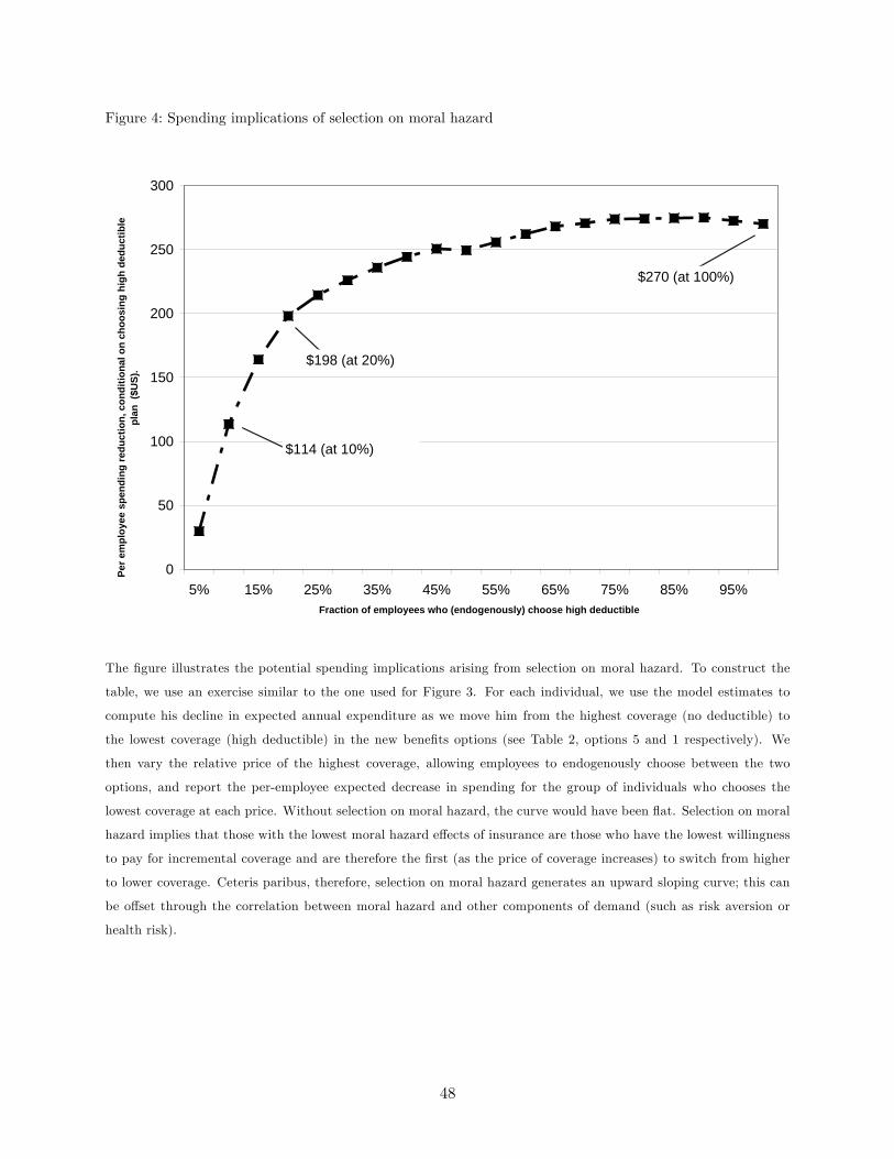
Figure 4: Spending implications of selection on moral hazard

0

50

100

150

200

250

300

5% 15% 25% 35% 45% 55% 65% 75% 85% 95%Fraction of employees who (endogenously) choose high deductible

Per e

mpl

oyee

 spe

ndin

g re

duct

ion,

 con

ditio

nal o

n ch

oosi

ng h

igh 

dedu

ctib

lepl

an  (

$US)

.

$114 (at 10%)

$270 (at 100%)

$198 (at 20%)

The figure illustrates the potential spending implications arising from selection on moral hazard. To construct the

table, we use an exercise similar to the one used for Figure 3. For each individual, we use the model estimates to

compute his decline in expected annual expenditure as we move him from the highest coverage (no deductible) to

the lowest coverage (high deductible) in the new benefits options (see Table 2, options 5 and 1 respectively). We

then vary the relative price of the highest coverage, allowing employees to endogenously choose between the two

options, and report the per-employee expected decrease in spending for the group of individuals who chooses the

lowest coverage at each price. Without selection on moral hazard, the curve would have been flat. Selection on moral

hazard implies that those with the lowest moral hazard effects of insurance are those who have the lowest willingness

to pay for incremental coverage and are therefore the first (as the price of coverage increases) to switch from higher

to lower coverage. Ceteris paribus, therefore, selection on moral hazard generates an upward sloping curve; this can

be offset through the correlation between moral hazard and other components of demand (such as risk aversion or

health risk).

48

Table 1: Summary statistics for 2003 sample

Obs. Average Age Average AnnualIncome

Average Tenurewith Alcoa Fraction Male Fraction White Fraction Single

Coverage

Avg number ofinsured family

members (if non­single coverage)

Total annualmedical spending

(US$)

(1) (2) (3) (4) (5) (6) (7) (8) (9)

Baseline sample 3,996 41.3 31,292 10.2 0.84 0.72 0.23 2.8 5,282

Switched in 2004 683 44.5 39,715 15.5 0.96 0.85 0.21 2.7 5,194Switched in 2005 974 39.7 25,532 8.2 0.73 0.44 0.25 2.8 5,364Switched in 2006 1,075 38.3 29,952 5.7 0.86 0.82 0.23 2.9 5,927Switched after 2006 1,264 43.3 32,316 12.7 0.85 0.79 0.22 2.6 4,717

Top row presents statistics based on the 2003 data for our baseline sample, which covers all hourly union workers not

covered by the Master Steelworker’s Agreement (except those that get dropped in the process of the data cleaning

described in the text). The subsequent rows (“Switched in 2004,” “Switched in 2005,” and so on) partition our

baseline sample based on the year in which employees were switched to the new set of health insurance options. Total

annual medical spending in column (9) is for employees and any covered dependents.

49

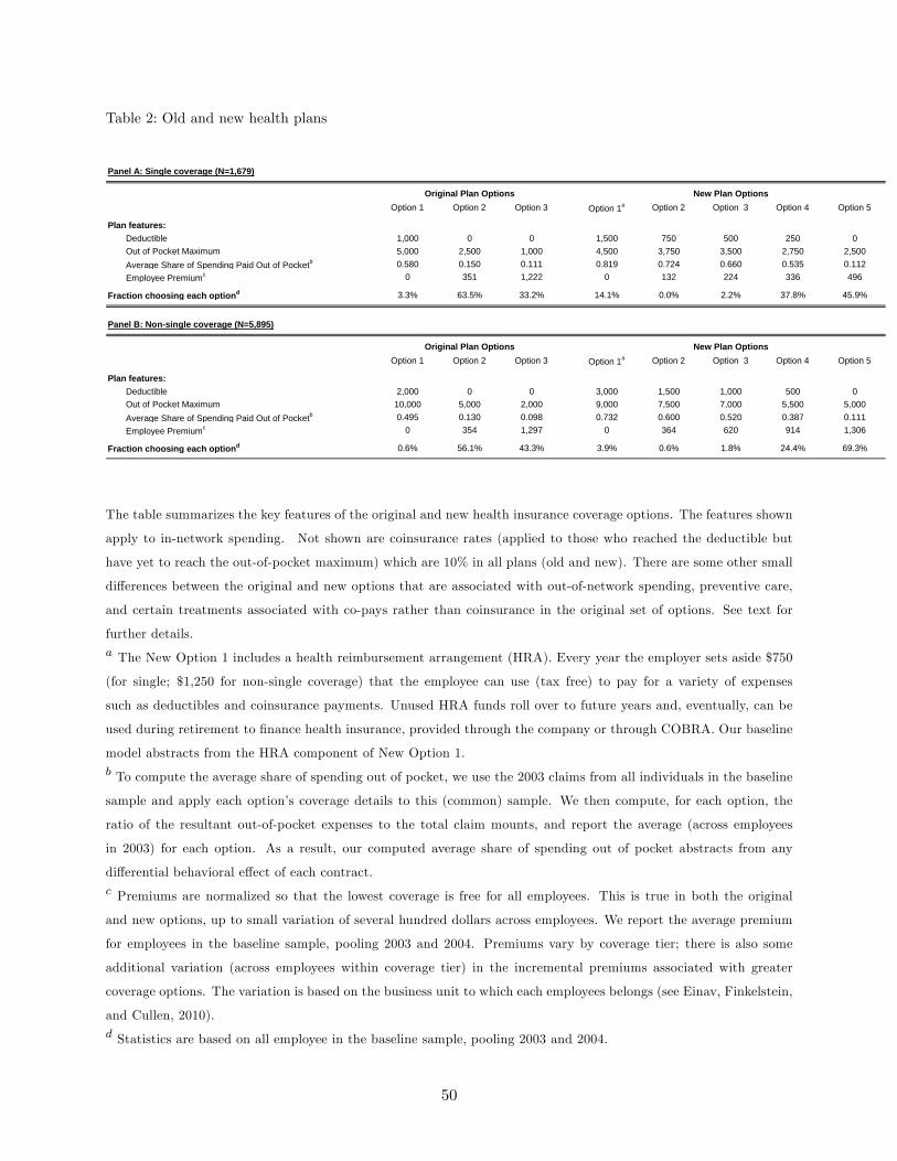
Table 2: Old and new health plans

Panel A: Single coverage (N=1,679)

Option 1 Option 2 Option 3 Option 1a Option 2 Option  3 Option 4 Option 5

Plan features:Deductible 1,000 0 0 1,500 750 500 250 0Out of Pocket Maximum 5,000 2,500 1,000 4,500 3,750 3,500 2,750 2,500Average Share of Spending Paid Out of Pocketb 0.580 0.150 0.111 0.819 0.724 0.660 0.535 0.112Employee Premiumc 0 351 1,222 0 132 224 336 496

Fraction choosing each optiond 3.3% 63.5% 33.2% 14.1% 0.0% 2.2% 37.8% 45.9%

Panel B: Non­single coverage (N=5,895)

Option 1 Option 2 Option 3 Option 1a Option 2 Option  3 Option 4 Option 5

Plan features:Deductible 2,000 0 0 3,000 1,500 1,000 500 0Out of Pocket Maximum 10,000 5,000 2,000 9,000 7,500 7,000 5,500 5,000Average Share of Spending Paid Out of Pocketb 0.495 0.130 0.098 0.732 0.600 0.520 0.387 0.111Employee Premiumc 0 354 1,297 0 364 620 914 1,306

Fraction choosing each optiond 0.6% 56.1% 43.3% 3.9% 0.6% 1.8% 24.4% 69.3%

Original Plan Options New Plan Options

Original Plan Options New Plan Options

The table summarizes the key features of the original and new health insurance coverage options. The features shown

apply to in-network spending. Not shown are coinsurance rates (applied to those who reached the deductible but

have yet to reach the out-of-pocket maximum) which are 10% in all plans (old and new). There are some other small

differences between the original and new options that are associated with out-of-network spending, preventive care,

and certain treatments associated with co-pays rather than coinsurance in the original set of options. See text for

further details.a The New Option 1 includes a health reimbursement arrangement (HRA). Every year the employer sets aside $750

(for single; $1,250 for non-single coverage) that the employee can use (tax free) to pay for a variety of expenses

such as deductibles and coinsurance payments. Unused HRA funds roll over to future years and, eventually, can be

used during retirement to finance health insurance, provided through the company or through COBRA. Our baseline

model abstracts from the HRA component of New Option 1.b To compute the average share of spending out of pocket, we use the 2003 claims from all individuals in the baseline

sample and apply each option’s coverage details to this (common) sample. We then compute, for each option, the

ratio of the resultant out-of-pocket expenses to the total claim mounts, and report the average (across employees

in 2003) for each option. As a result, our computed average share of spending out of pocket abstracts from any

differential behavioral effect of each contract.c Premiums are normalized so that the lowest coverage is free for all employees. This is true in both the original

and new options, up to small variation of several hundred dollars across employees. We report the average premium

for employees in the baseline sample, pooling 2003 and 2004. Premiums vary by coverage tier; there is also some

additional variation (across employees within coverage tier) in the incremental premiums associated with greater

coverage options. The variation is based on the business unit to which each employees belongs (see Einav, Finkelstein,

and Cullen, 2010).d Statistics are based on all employee in the baseline sample, pooling 2003 and 2004.

50

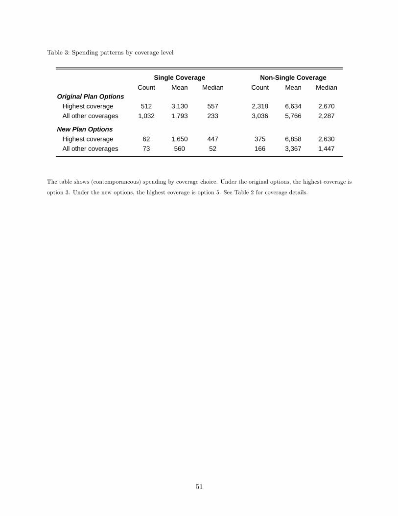
Table 3: Spending patterns by coverage level

Count Mean Median Count Mean MedianOriginal Plan Options   Highest coverage 512 3,130 557 2,318 6,634 2,670   All other coverages 1,032 1,793 233 3,036 5,766 2,287

New Plan Options   Highest coverage 62 1,650 447 375 6,858 2,630   All other coverages 73 560 52 166 3,367 1,447

Single Coverage Non­Single Coverage

The table shows (contemporaneous) spending by coverage choice. Under the original options, the highest coverage is

option 3. Under the new options, the highest coverage is option 5. See Table 2 for coverage details.

51

Table 4: Basic difference-in-differences in baseline sample

Obs. Mean Fraction with zerospending 10th 25th 50th 75th 90th

Control (Switched after 2004)2003 spending 3,313 5,300 0.09 52 426 1,775 5,178 11,9842004 spending 2,902 5,248 0.09 55 516 1,888 5,589 12,253

Treated (Switched in 2004)2003 spending 683 5,194 0.08 79 579 1,956 5,048 12,6442004 spending 676 4,843 0.10 0 447 1,601 4,615 9,468

2003 spending ­106 ­0.01 27 153 181 ­130 6602004 spending ­405 0.01 ­55 ­69 ­287 ­974 ­2,785

2004­2003 Difference (levels)Control (switched after 2004) ­52 0.00 3 90 113 411 269Treated (Switched in 2004) ­351 0.02 ­79 ­132 ­355 ­433 ­3,176

­299 0.02 ­82 ­222 ­468 ­844 ­3,445

Difference (percentages)Control (switched after 2004) ­1.0% 0.0% 5.8% 21.1% 6.4% 7.9% 2.2%Treated (Switched in 2004) ­6.8% 25.0% ­100.0% ­22.8% ­18.1% ­8.6% ­25.1%Diff. in differences ­5.8% 25.0% ­105.8% ­43.9% ­24.5% ­16.5% ­27.4%

Treated­Control Differences (levels)

Difference in differences (levels)

52

Table 5: Difference-in-differences estimates of impact of change in health insurance options on annual medical

spending

OLS in levels OLS in logs QMLE­Poisson OLS in levels OLS in logs QMLE­Poisson(1) (2) (3) (4) (5) (6)

Estimated Treatment effect ­301.9 ­0.356 ­0.061 ­591.8 ­0.175 ­0.114(752.6) (0.19) (0.15) (264.2) (0.12) (0.048)[0.69] [0.07] [0.69] [0.034] [0.17] [0.018]

Mean Dependent Variable 5,230 6.91 5,230 5,392 6.9 5,392N 7,574 7,574 7,574 14,638 14,638 14,638

2003­2004 sample 2003­2006 sample

The table shows the difference-in-difference estimate of the spending reduction associated with moving from the old

options to the new options. The unit of observation is an employee-year. Dependent variable is the total annual

medical spending for each employee and any covered dependents (or log of 1 + total spending in column (2) and

column (5)). The coeffi cient shown is the coeffi cient on an indicator variable that is equal to 1 if the employee’s

treatment group is offered the new health insurance options that year, and 0 otherwise. All regressions include year

and treatment group fixed effects. We classify employees into one of four possible treatment groups - switched in 2004,

switched in 2005, switched in 2006, or switched later - based on his union affi liation which determines the year in

which he is switched to the new health insurance options. Estimation is either by OLS or QMLE Poisson as indicated

in the column headings. Standard errors (in parentheses) are adjusted for an arbitrary variance-covariance matrix

within each of the 28 unions; p-values are in [square brackets]. Columns (1)-(3) show estimates for the 2003-2004

sample; Columns (3)-(6) expand the sample to include 2003-2006.

53

Table 6: Suggestive evidence of heterogeneous moral hazard and of selection on moral hazard

Coeff. Std. Err.(1) (2) (3) (4) (5) (6) (7)

Above median age (of 43) 6,972 6,263 ­1,302 (799) 12.4 27.8 15.4

Below or equal to median age (of 43) 7,666 4,600 ­85.8 (483) 12.9 29.5 16.6

Male 12,373 5,442 ­604 (293) 12.6 29.1 16.5

Female 2,265 5,120 ­579 (693) 12.9 25.8 12.9

Above median income (of $31,000) 7,322 5,669 ­364 (602) 12.2 29.1 16.9

Below median income (of $31,000) 7,316 5,116 ­301 (397) 13 28.1 15.1

Less coverage in 2003 6,997 5,003 ­621 (513) 13.4 32 18.6

More coverage in 2003 5,229 6,296 ­1,336 (596) 10.1 23.5 13.4

(A)

(B)

(C)

(D)

Obs. Meanspending

Avg Out­of­Pocket Share(Old Options)

Increase inOut­of­Pocket

Share

Avg Out­of­PocketShare (New

Options)

Estimated change in spending associatedwith change in options (levels)

The table shows results for different groups of workers (shown in different rows) in the 2003-2006 sample. Column

(1) reports the number of employee-years in the sample, and column (2) reports their mean annual medical spending

over the sample period. Columns (3) and (4) report, respectively, the coeffi cient and standard error of the estimated

change in spending associated with moving from the old to the new options. This is based on a difference-in-differences

regression on the 2003-2006 sample; we report in columns (3) and (4) the coeffi cient and standard error on an indicator

variable that is equal to 1 if the employee’s treatment group is offered the new health insurance options that year,

and 0 otherwise. The dependent variable is always total annual medical spending for each employee and any covered

dependents. All regressions include year and treatment group fixed effects. Standard errors (in parentheses) are

adjusted for an arbitrary variance-covariance matrix within each of the 28 unions. Columns (5) and (6) show the

average out of pocket share within each group under the old and new options respectively. These are calculated based

on the share of employees within each group in each plan, and the plan specific out of pocket shares shown in Table 2

(which are computed on a common sample of workers across plans). Column (7) reports the increase in the average

out of pocket share for each group associated with moving from the old options to the new options. In panel (D), the

sample is limited to employees who are employed at the firm in 2003 and who choose either “more coverage”(option

3 from Table 2) or “less coverage”(option 2 from Table 2) in 2003.

54

Table 7: Parameter estimates

Mean ShiftersMu_Lambda Kappa_Lambda Omega Psi(Health risk) (Health risk) (Moral hazard) (Risk aversion)

Constant 5.88 (0.086) 264 (38) 5.29 (0.14) ­5.50 (0.06)

Coverage tier   Single (omitted) (omitted) (omitted) (omitted)   Family 1.60 (0.078) ­261 (37) 0.75 (0.17) ­1.47 (0.05)   Emp+Spouse 1.60 (0.084) ­73 (58) 0.56 (0.32) ­1.46 (0.06)   Emp+Children 0.85 (0.091) ­258 (47) ­0.22 (0.28) ­1.13 (0.06)

Switch group   Switch 2004 0.13 (0.075) 297 (51) ­0.40 (0.20) ­0.40 (0.05)   Switch 2005 0.08 (0.073) 161 (43) 0.15 (0.17) ­0.40 (0.05)   Switch 2006 0.14 (0.074) 92 (43) ­0.20 (0.19) ­0.10 (0.05)   Switch later (omitted) (omitted) (omitted) (omitted)

2004 Time dummy ­0.10 (0.020) ­­ ­­

Variance­covariance matrixMu_Lambda Omega Psi(Health risk) (Moral hazard) (Risk aversion)

Mu_Lambda 0.52 (0.06) 0.23 (0.08) ­0.14 (0.04)Omega ­­ 2.01 (0.15) ­0.16 (0.06)Psi ­­ ­­ 0.19 (0.02)

Additional parametersSigma_Mu_Bar 0.78 (0.04)Sigma_Kappa 0.44 (0.06)Gamma1 (Sigma_Lambda parameter) 0.0092 (0.0013)Gamma2 (Sigma_Lambda parameter) 49 (4.1)

Implied quantitiesLambda Omega Psi

(Health risk) (Moral hazard) (Risk aversion)Expected 5,620 822 0.00156Std. Dev. 40,200 2,426 0.00151

The table presents our baseline parameter estimates based on our baseline sample of 7,572 employees. As described

in the text, the estimates are based on a Gibbs sampler; the table reports the posterior mean and the posterior

standard deviations in parentheses. Bottom panel reports some implied quantities of interest that are derived from

the estimated parameters.

55

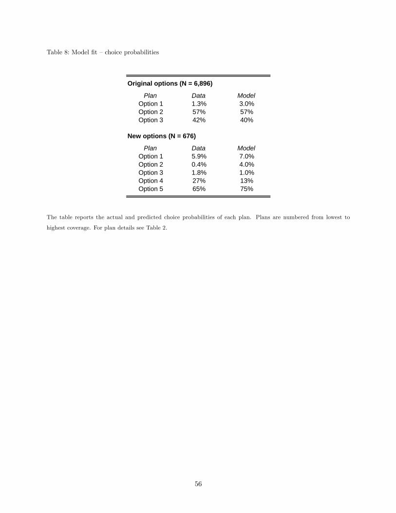
Table 8: Model fit —choice probabilities

Original options (N = 6,896)

Plan Data ModelOption 1 1.3% 3.0%Option 2 57% 57%Option 3 42% 40%

New options (N = 676)

Plan Data ModelOption 1 5.9% 7.0%Option 2 0.4% 4.0%Option 3 1.8% 1.0%Option 4 27% 13%Option 5 65% 75%

The table reports the actual and predicted choice probabilities of each plan. Plans are numbered from lowest to

highest coverage. For plan details see Table 2.

56

Table 9: Spending implications of moral hazard estimates

Mean Std. Dev. 10th 25th 50th 75th 90th

Spending difference as we movefrom no to high deductible plan 270 571 0 0 37 273 787

Spending difference as we movefrom full to no insurance 790 2,427 0 64 237 703 1,777

The table reports the implied spending implications if we move different employees across plans. For each employee,

we use the model estimates to compute his decline in expected annual expenditure as we change his insurance plan.

In the top row, we move each employee from the highest coverage option under the new benefit options (option 5)

to the lowest coverage option under the new benefit options (option 1); roughly speaking, this entails moving from

a plan with no deducible to a plan with a high deductible; see Table 2 for more details. In the bottom row, we

move each employee from full to no insurance. The table then summarizes the cross-sectional distribution of the

spending effects. The estimates are primarily driven by the estimated distribution of ω, but they take into account

the truncation of spending at zero by integrating over the conditional (on ω) distribution of λ.

57

Table 10: Spending and welfare effects of asymmetric information

Average equilibrium(incremental) premium

No deductible planshare

Expected spending peremployee

Total welfare peremployee

(1) "Status quo": no screening or monitoring 2,737 0.41 5,725 normalized to 0

(2) "Perfect screening": premiums depend onF(lambda) and omega 1,465 0.93 5,846 458

(3) "Imperfect screening": premiums dependon omega (but not on F(lambda)) 2,649 0.43 5,706 45

(4) "Perfect monitoring": contracts reimburseonly "lambda­related" spending 2,566 0.46 5,183 211

(5) "Imperfect monitoring": perfect monitoringassumed for choice (but not for utilization) 2,566 0.46 5,737 57

The table reports the spending and welfare effects from a set of counterfactual contracts described in the text. All

exercises are applied to a setting in which the only two options available are the no deductible plan and the high

deductible plan under the new benefit options (i.e. option 5 and option 1, respectively; see Table 2). Equilibrium

premiums are computed as the incremental (relative) premium for the no deductible plan that equals the expected

incremental costs associated with providing the no deductible plan to those who choose it. The no deductible plan

share is calculated based on the choice probabilities as a function of equilibrium premiums. Expected spending

and total welfare are computed based on these choices. Row 1 assumes the “status quo” asymmetric information

contracts, which a “uniform” price that varies only by coverage tier. Row 2 assumes “perfect screening”, so that

contracts are priced based on ωi and all components of Fi(λ) and adverse selection is eliminated. Row 3 assumes

“imperfect screening”, in which contracts are priced based only on ωi.Row 4 assumes “perfect monitoring”so that

moral hazard is eliminated. Specifically we assume the insurance provider can counterfactually observe (and not

reimburse) spending that is associated with moral hazard; spending associated with health —realization of λ —are

reimbursed according to the observed contracts. Row 5 assumes “imperfect monitoring”in which, ex ante individuals

choose contracts under the assumption that there will be perfect monitoring (i.e. spending associated with moral

hazard will not be reimbursed), but ex-post (after they choose their contract but before they make their spending

decision) the contracts are changed to be the standard contracts that reimburse all medical spending regardless of its

origin.

58

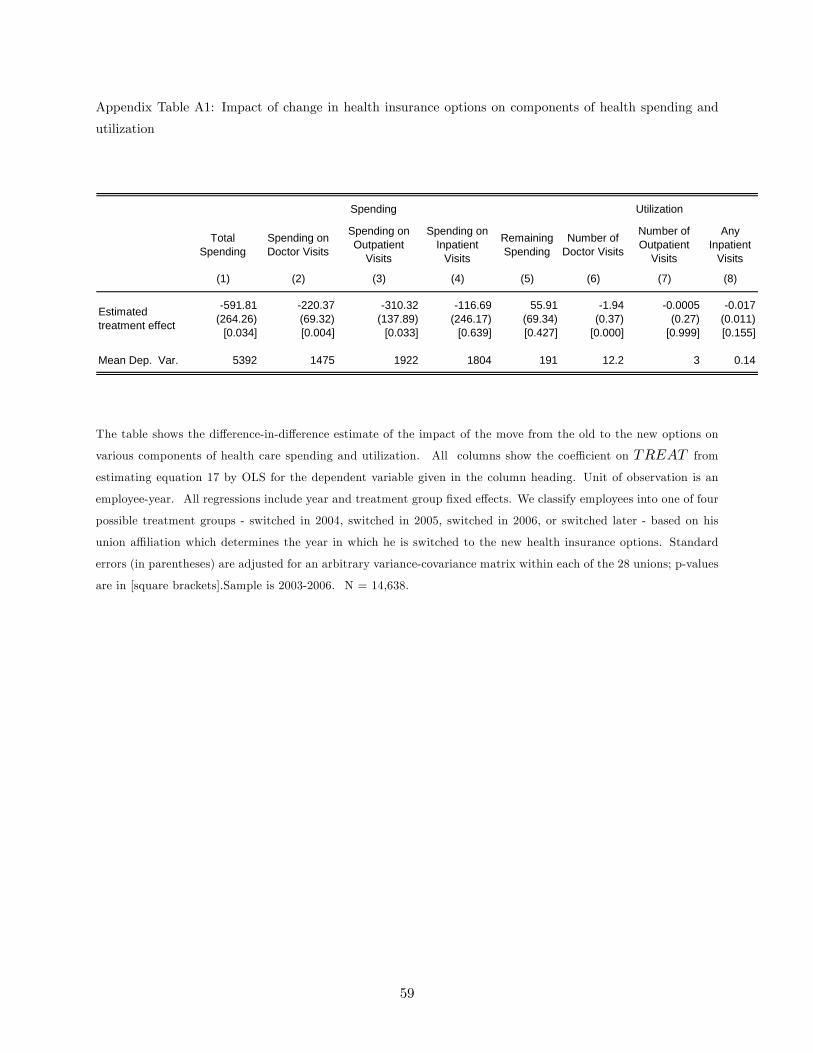
Appendix Table A1: Impact of change in health insurance options on components of health spending and

utilization

TotalSpending

Spending onDoctor Visits

Spending onOutpatient

Visits

Spending onInpatient

Visits

RemainingSpending

Number ofDoctor Visits

Number ofOutpatient

Visits

AnyInpatient

Visits

(1) (2) (3) (4) (5) (6) (7) (8)

­591.81 ­220.37 ­310.32 ­116.69 55.91 ­1.94 ­0.0005 ­0.017(264.26) (69.32) (137.89) (246.17) (69.34) (0.37) (0.27) (0.011)

[0.034] [0.004] [0.033] [0.639] [0.427] [0.000] [0.999] [0.155]

Mean Dep.  Var. 5392 1475 1922 1804 191 12.2 3 0.14

UtilizationSpending

Estimatedtreatment effect

The table shows the difference-in-difference estimate of the impact of the move from the old to the new options on

various components of health care spending and utilization. All columns show the coeffi cient on TREAT from

estimating equation 17 by OLS for the dependent variable given in the column heading. Unit of observation is an

employee-year. All regressions include year and treatment group fixed effects. We classify employees into one of four

possible treatment groups - switched in 2004, switched in 2005, switched in 2006, or switched later - based on his

union affi liation which determines the year in which he is switched to the new health insurance options. Standard

errors (in parentheses) are adjusted for an arbitrary variance-covariance matrix within each of the 28 unions; p-values

are in [square brackets].Sample is 2003-2006. N = 14,638.

59

Appendix Table A2: Impact of change in health insurance options on spending (quarterly data)

BaselinePre­

specificationtest

BaselinePre­

specificationtest

Col (4) w treatment­group­specific linear

trendMore dynamics

(1) (2) (3) (4) (5) (6)

TREATjt ­147.87 ­139.44 ­156.85 ­157.54 ­185.65(66.04) (85.22) (43.60) (50.49) (74.82)[0.034] [0.113] [0.001] [0.004] [0.020]

TREATjt,0 40.78 ­3.31 ­5.69(158.49) (69.21) (76.00)

[0.799] [0.962] [0.941]

TREATjt,­3 58.59(60.91)

TREATjt,­2 ­2.46(90.69)

TREATjt,­1 ­42.03(69.75)

TREATjt,0 0 (reference period)

TREATjt,1 ­121.79(53.47)

TREATjt,2 ­187.06(77.21)

TREATjt,3 ­118.35(65.90)

TREATjt,4 ­197.82(61.78)

Mean dep. Var.

Total Spending

1348

Total Spending, Censored at 99th percentile

1125

The table shows the difference-in-difference estimate of the impact of the move from the old to the new options.

Specifically, columns 1 through 5 show the results from estimating equation 18 (and column 6 shows results from

estimating equation 19) by OLS for the dependent variable total quarterly health spending. Unit of observation is an

employee-quarter. The variable TREATjt is an indicator variable for whether treatment group j is offered the new

health insurance options in quarter t. The variable Treatjt,0 is an indicator variable for whether it is the quarter

before group j is switched to the new health insurance options. The variable TREATjt,k is an indicator variable

for whether it is k quarters since quarter 0 (i.e. the quarter before the switch). All regressions include quarter and

treatment group fixed effects; column 5 also includes a treatment group-specific linear trend. We classify employees

60

into one of four possible treatment groups - switched in 2004, switched in 2005, switched in 2006, or switched later -

based on his union affi liation which determines the year in which he is switched to the new health insurance options.

Standard errors (in parentheses) are adjusted for an arbitrary variance-covariance matrix within each of the 28 unions;

p-values are in [square brackets].Sample is 2003-2006. N = 58,552.

61

Appendix Table A3: Sensitivity of annual difference-in-differences estimates to controlling for observables

Baseline (nocovariates)

Adding controlfor coverage

tier

Addingadditional

demographiccontrols

At Alcoa allfour years

At Alcoa all fouryears, w individual

fixed effects.

(3) (2) (3) (4) (5)

TREATjt ­591.81 ­522.74 ­537.96 ­965.92 ­965.92(264.26) (267.29) (264.33) (302.33) (349.04)

[0.034] [0.061] [0.052] [0.004] [0.012]

Mean Dep. Var.N

539214,638 7,580

5438

The table examines the sensitivity of the annual difference-in-differences estimates of the impact of the move from

the old to the new options on total annual medical spending. All columns show the coeffi cient on TREAT from

estimating equation 17 by OLS for the dependent variable total annual medical spending. Unit of observation is an

employee-year. All regressions include quarter and treatment group fixed effects. We classify employees into one of

four possible treatment groups - switched in 2004, switched in 2005, switched in 2006, or switched later - based on

his union affi liation which determines the year in which he is switched to the new health insurance options. Standard

errors (in parentheses) are adjusted for an arbitrary variance-covariance matrix within each of the 28 unions; p-values

are in [square brackets].Sample is 2003-2006. Column 1 replicates the baseline results (from Table 5, column 4).

In column 2 we control for coverage tier. In column 3 we control for coverage tier, employee age, employee gender,

number of dependents insured on the policy, whether the employee is white, the number of years the employee has

been at Alcoa, and the employee’s annual salary. Column 4 limits the sample to employees who are at Alcoa (and in

our data) for all four years. Column 5 adds employee fixed effects to the sample in column 4.

62

Appendix Table A4: Additional sensitivity analysis

Baseline quarterlyspecification (OLS)

GLS estimation atTreatment group ­

quartelry level(1) (2) (3)

TREATjt ­0.021 ­147.87 ­166.43(0.024) (66.04) (61.22)[0.376] [0.034] [0.007]

Mean dep var 0.106 1348 1364N 16366 58,552 64

Dependentvariable:  choose a

non­PPO option

Dependent variable: total spending

The table examines some additional sensitivity of the annual difference-in-differences estimates of the impact of the

move from the old to the new options on total annual medical spending. All regressions include year and treatment

group fixed effects. Column 1 shows the coeffi cient on TREAT from estimating equation 17 by OLS on the baseline

2003-2006 sample, plus the employees who choose a non-PPO option; the dependent variable is an indicator variable

for whether the employee chose a non PPO option; unit of observation is an employee-year. In columns 2 and 3 the

dependent variable is total spending. Column 2 shows the coeffi cient on TREAT from estimating equation 18 by

OLS at the employee-quarter level. Column 3 shows the coeffi cient on TREAT from estimating equation 18 by

GLS with a panel-specific auto correlation parameter and variance at the treatment group - quarter level. In columns

1 and 2 standard errors (in parentheses) are adjusted for an arbitrary variance-covariance matrix within each of the

28 unions; p values are in [square brackets].

63