Seediscussions,stats,andauthorprofilesforthispublicationat:https://www.researchgate.net/publication/307420414

SelectingandevaluatingCCVAapproachesandmethods

Chapter·August2016

CITATIONS

0

READS

78

6authors,including:

Someoftheauthorsofthispublicationarealsoworkingontheserelatedprojects:

REDD+readinesspilotprojectinTanzania-EnhancingTanzanianCapacitytoDeliverShortandLong

TermonForestCarbonStocksAcrosstheCountryViewproject

landuse-climatescenarios,biodiversity-foodsecuritytrade-offsViewproject

WendyFoden

StellenboschUniversity

80PUBLICATIONS1,256CITATIONS

SEEPROFILE

RaquelA.Garcia

StellenboschUniversity

25PUBLICATIONS398CITATIONS

SEEPROFILE

PhilipJPlatts

TheUniversityofYork

71PUBLICATIONS708CITATIONS

SEEPROFILE

PieroVisconti

UNEPWorldConservationMonitoringCentre

62PUBLICATIONS2,060CITATIONS

SEEPROFILE

AllcontentfollowingthispagewasuploadedbyPhilipJPlattson05September2016.

Theuserhasrequestedenhancementofthedownloadedfile.

Produced with support fromIUC

N

INTERNATIONAL UNIONFOR CONSERVATION OF NATURE

World Headquartersrue Mauverney 281196 Gland, switzerlandtel: +41 22 999 0000Fax: +41 22 999 0002www.iucn.org

IuCN ssC Guidelines for assessing species’ Vulnerability to Climate Changeeditors: Wendy B. Foden and Bruce e. Young

IuC

N s

sC

Guidelines for a

ssessing species’ Vulnerability to C

limate C

hange

Occasional Paper of the IUCN Species Survival Commission No. 59

About IUCN

IUCN is a membership Union uniquely composed of both government and civil society organizations. It provides public, private and non-governmental organizations with the knowledge and tools that enable human progress, economic development and nature conservation to take place together.

Created in 1948, IUCN is now the world’s largest and most diverse environmental network, harnessing the knowledge, resources and reach of 1,300 member organizations and some 15,000 experts. It is a leading provider of conservation data, assessments and analysis. Its broad membership enables IUCN to fill the role of incubator and trusted repository of best practices, tools and international standards.

IUCN provides a neutral space in which diverse stakeholders including governments, NGOs, scientists, businesses, local communities, indigenous peoples organizations and others can work together to forge and implement solutions to environmental challenges and achieve sustainable development.

Working with many partners and supporters, IUCN implements a large and diverse portfolio of conservation projects worldwide. Combining the latest science with the traditional knowledge of local communities, these projects work to reverse habitat loss, restore ecosystems and improve people’s well-being.

www.iucn.org

IUCN SSC Guidelines for Assessing Species’ Vulnerability to Climate Change

Occasional Paper of the IUCN Species Survival Commission No. 59

Produced with support from

IUCN SSC Guidelines for Assessing Species’ Vulnerability to Climate ChangeEditors: Wendy B. Foden and Bruce E. Young

iv

The designation of geographical entities in this document, and the presentation of the material, do not imply the expression of any opinion whatsoever on the

part of IUCN or the organisations of the authors and editors of the document concerning the legal status of any country, territory, or area, or of its authorities,

or concerning the delimitation of its frontiers or boundaries.

The views expressed in this publication do not necessarily reflect those of IUCN.

Published by: IUCN, Cambridge, UK and Gland, Switzerland

Copyright: © 2016 International Union for Conservation of Nature and Natural Resources

Reproduction of this publication for educational or other non-commercial purposes is authorized without prior written

permission from the copyright holder provided the source is fully acknowledged.

Reproduction of this publication for resale or other commercial purposes is prohibited without prior written permission of

the copyright holder.

Citation: Foden, W.B. and Young, B.E. (eds.) (2016). IUCN SSC Guidelines for Assessing Species’ Vulnerability to Climate Change.

Version 1.0. Occasional Paper of the IUCN Species Survival Commission No. 59. Cambridge, UK and Gland, Switzerland:

IUCN Species Survival Commission. x+114pp.

Suggested chapter citation (example) Huntley, B., Foden, W.B., Smith, A., Platts, P., Watson, J. and Garcia, R.A. (2016). Chapter 5. Using CCVAs and interpreting

their results. In W.B. Foden and B.E. Young, editors. IUCN SSC Guidelines for Assessing Species’ Vulnerability to Climate

Change. Version 1.0. Occasional Paper of the IUCN Species Survival Commission No. 59. Gland, Switzerland and Cambridge,

UK. pp 33–48.

Available online at: http://www.iucn.org/theme/species/publications/guidelines and www.iucn-ccsg.org

ISBN: 978-2-8317-1802-6

DOI: http://dx.doi.org/10.2305/IUCN.CH.2016.SSC-OP.59.en

Cover photo: Polar Bear near Svalbard, Norway. © Josef Friedhuber, Getty Images.

All photographs used in this publication remain the property of the original copyright holder (see individual captions for details). Photographs should not be

reproduced or used in other contexts without written permission from the copyright holder.

Layout by: NatureBureau

Printed by: Langham Press

Available from: IUCN (International Union for Conservation of Nature), Global Species Programme, 28 Rue Mauverney, 1196 Gland,

Switzerland. Tel: + 41 22 999 0000, Fax: + 44 22 999 0002, www.iucn.org/resources/publications

v

Contents

Working group ........................................................................................................................................................................... viiiEditors and authors ....................................................................................................................................................................... ixAcknowledgements ........................................................................................................................................................................ x

1. Introduction ...........................................................................................................................................................................1

2. Settingthescene ....................................................................................................................................................................5 2.1 Definitions of commonly used terms ................................................................................................................................ 5 2.2 Climate change vulnerability assessment approaches ......................................................................................................... 8 2.2.1 Correlative approaches ............................................................................................................................................. 8 2.2.2 Trait-based approaches ............................................................................................................................................. 9 2.2.3 Mechanistic approaches ........................................................................................................................................... 9 2.2.4 Combined approaches ........................................................................................................................................... 10 2.3 Metrics for estimating climate change vulnerability .......................................................................................................... 11 2.3.1 Vulnerability indices and other relative scoring systems ........................................................................................ 11 2.3.2 Range changes ....................................................................................................................................................... 11 2.3.4 Population changes ................................................................................................................................................ 11 2.3.5 Extinction probabilities .......................................................................................................................................... 11

3. Settingclimatechangevulnerabilityassessmentgoalsandobjectives ............................................................................13 3.1 Defining your goal .......................................................................................................................................................... 13 3.1.1 Why are you carrying out this CCVA? ................................................................................................................... 13 3.1.2 Who is your audience? ........................................................................................................................................... 13 3.1.3 Which decisions do you hope to influence using the results? ................................................................................. 13 3.2 Defining your objectives ................................................................................................................................................. 14 3.2.1 Selecting a taxonomic focus ................................................................................................................................... 14 3.2.2 Selecting a spatial focus ......................................................................................................................................... 14 3.2.3 Selecting a timeframe ............................................................................................................................................ 14

4. SelectingandevaluatingCCVAapproachesandmethods ............................................................................................... 17 4.1 Steps for selecting your CCVA approach and methods ................................................................................................... 17 Step 1. Identify and evaluate existing CCVAs ................................................................................................................ 17 Step 2. Identify CCVA approaches that meet your objectives ......................................................................................... 18 Step 3. Identify the CCVA approaches for which you have sufficient resources .............................................................. 19 Step 4. Do Steps 2 and 3 identify any of the same approaches? ...................................................................................... 26 Step 5. Select your approach(es) and the methods for applying it/them .......................................................................... 26 4.2 Approaches for three challenging CCVA situations: poorly-known, small- and declined-range species ..................................28

5. UsingCCVAsandinterpretingtheirresults ......................................................................................................................33 5.1 Selecting and using input data ........................................................................................................................................ 33 5.1.1 Spatial extent and resolution................................................................................................................................... 33 5.1.2 Time frames ........................................................................................................................................................... 34 5.1.3 Climate datasets ..................................................................................................................................................... 34 5.1.4 Species distribution data ......................................................................................................................................... 39 5.1.5 Species trait data ..................................................................................................................................................... 39 5.1.6 Accounting for habitat availability ......................................................................................................................... 45 5.2 Challenges to applying current CCVA approaches ............................................................................................................ 46 5.2.1 Direct versus indirect impacts of climate change ..................................................................................................................46 5.2.2 Interpreting spatially explicit model outputs ............................................................................................................. 46

6. Understandingandworkingwithuncertainty .................................................................................................................49 6.1 Uncertainty from species’ distribution and abundance data ........................................................................................... 49 6.2 Uncertainty from climate projections and baseline datasets ........................................................................................... 50 6.3 Uncertainty from choice of bioclimatic variables ............................................................................................................ 50 6.4 Uncertainty from potentially incomplete evidence of species’ niches ....................................................................................... 51

vi

6.5 Uncertainty from biological trait and demographic data ................................................................................................ 51 6.5.1 Changes in traits over time..................................................................................................................................... 52 6.6 Uncertainty from choice of method ................................................................................................................................ 52 6.6.1 Correlative approaches ........................................................................................................................................... 52 6.6.2 Trait-based approaches ........................................................................................................................................... 54 6.7 CCVA validation ............................................................................................................................................................ 54

7. TheIUCNRedListandClimateChangeVulnerability .............................................................................................................57 7.1 Using CCVA results for IUCN Red Listing ................................................................................................................... 57 7.2 Three user scenarios for Red Listing considering climate change .................................................................................... 58

8. CommunicatingCCVAresults ........................................................................................................................................... 61

9. FuturedirectionsinCCVAofspecies ................................................................................................................................63 9.1 Validation of assessments ................................................................................................................................................ 63 9.2 Better and more coordinated biodiversity data ............................................................................................................... 63 9.3 Advancing CCVA methodology ..................................................................................................................................... 63 9.3.1 Combination or ‘hybrid’ methods that draw on the strengths of different approaches .......................................... 63 9.3.2 Including the effects of changing frequency and magnitude of climate extremes and variability ............................... 63 9.3.3 Including inter-species interactions ........................................................................................................................64 9.3.4 Including human responses to climate change ........................................................................................................64 9.3.5 Including interactions between climate change and other threats ..........................................................................64 9.3.6 Accounting for climate change-driven species changes that have already occurred ...............................................64 9.3.7 Improving trait data and selection of thresholds for vulnerability ..........................................................................64 9.3.8 Incorporating adaptive genetic change and phenotypic plasticity ..........................................................................64 9.3.9 Taking advantage of advances in -omics and next generation sequencing .............................................................. 65 9.4 Improved information exchange between conservation research and practitioner communities .................................... 65 9.5 Better use of CCVA to inform conservation planning ....................................................................................................... 66 9.6 Explore the links between CCVA of species and implications for people........................................................................ 66

10.CaseStudies .........................................................................................................................................................................67 Case Study 1. A correlative approach for Australian tropical savanna birds .......................................................................... 69 Case Study 2. Developing a framework for identifying climate change adaptation strategies for Africa’s Important Bird Area network ......................................................................................................................................... 71 Case Study 3. Back to basics with African amphibians ......................................................................................................... 74 Case Study 4. Exploring impacts of declining sea ice on polar bears and their ringed seal and bearded seal prey in the northern Barents Sea ............................................................................................................................................. 77 Case Study 5. Freshwater fishes in the Appalachian Mountains, USA .................................................................................. 81 Case Study 6. A trait-based CCVA of all warm-water reef-building corals globally .............................................................. 83 Case Study 7. Assessing climate change vulnerability of the West Africa protected area network for birds, mammals and amphibians ............................................................................................................................................................... 87 Case Study 8. Correlative-mechanistic CCVA of the Iberian Lynx ....................................................................................... 89 Case Study 9. Matching species traits to correlative model projections in a combined CCVA approach............................... 91 Case Study 10. A combined approach for CCVA of the Mountain Ringlet (Erebia epiphron) and Stag Beetle (Lucanus cervus) in Great Britain .................................................................................................................. 94

11.MainReferences ..................................................................................................................................................................97

vii

12.Appendix ............................................................................................................................................................................109 Appendix Table A. Examples of methods that have been used to apply a correlative approach to CCVA ........................... 109 Appendix Table B. Examples of methods that have been used to apply a trait-based approach to CCVA ............................110 Appendix Table C. Examples of methods that have been used to apply a mechanistic approach to CCVA. ........................110 Appendix Table D. Examples of methods that have been used to apply a combination approach to CCVA ........................111 Appendix References ........................................................................................................................................................... 112

Boxes Box 1. Literature resources for climate change adaptation and vulnerability assessment ......................................................... 3 Box 2. Comparison of climate change vulnerability terms currently in use ............................................................................ 5 Box 3. Types of species that pose challenges to CCVA .......................................................................................................... 22 Box 4. Selecting the method(s) for applying CCVA approaches ............................................................................................ 27 Box 5. Climate Change and the Guidelines for Using the IUCN Red List Categories and Criteria ..................................... 57 Box 6. The potential of –omics approaches for management of threatened species ............................................................... 65

MainTables Table 1. Checklist to aid identification of clear, quantitative objectives ................................................................................. 14 Table 2. Heuristic examples of CCVA objectives, grouped according to six objective categories, and their scope of focus ... 15 Table 3. Examples of species-level open-access CCVA studies and/or results ........................................................................ 18 Table 4. CCVA objective categories, examples of outputs required to meet them, and the approaches potentially able to deliver these ......................................................................................................................................................... 20 Table 5. Summary of the data resources generally required by each CCVA approach ........................................................... 21 Table 6. Examples of data resources available for use in CCVA ............................................................................................ 22 Table 7. Approaches for three challenging CCVA situations ................................................................................................. 30 Table 8. Examples of the most widely used and generally available climate datasets representing historical (baseline or recent past) climatic conditions ................................................................................................................... 36 Table 9. Trait categories associated with species’ heightened sensitivity and low adaptive capacity to climate change .......... 40 Table 10. Examples of the traits considered by five trait-based CCVAs ................................................................................. 41 Table 11. Examples of CCVA target audiences, the types of information they require, and some of the communication media that are useful for communicating CCVAs and their results to them ........................................ 61 Table 12. List of case studies and the approaches, ecosystems, spatial scales and resource scenarios they cover .................... 67 Table 13. Key to selecting case studies appropriate to your CCVA objectives ....................................................................... 68 Appendix Table A ................................................................................................................................................................ 109 Appendix Table B .................................................................................................................................................................110 Appendix Table C .................................................................................................................................................................110 Appendix Table D ................................................................................................................................................................111

MainFigures Figure 1. Target audiences of these guidelines ......................................................................................................................... 2 Figure 2. Schematic diagram showing three components of vulnerability in CCVAs ............................................................. 5 Figure 3. Risk of climate-related impacts ................................................................................................................................ 5 Figure 4. Five key parameters for describing vulnerability of biodiversity to climate change .................................................. 7 Figure 5. Summary of the three main CCVA approaches (1–3) and the six categories their combinations create ................... 8 Figure 6. The four main metrics or types of information derived from CCVA and the approaches that produce them ........ 11 Figure 7. Conceptual steps for CCVA of species .................................................................................................................... 17 Figure 8. Steps for evaluating the suitability of existing CCVA studies according to a consensus approach ......................... 19 Figure 9. Framework for interpreting the results of multiple CCVA approaches and methods ............................................. 27 Figure 10. Confusion matrix ................................................................................................................................................. 53

viii

Working Group

WendyB.Foden (University of Stellenbosch) (Chair)BruceE.Young (NatureServe) (Deputy Chair)

ResitAkçakaya (Stonybrook University)DavidBaker (University of Durham)DavidBickford (National University of Singapore)StuartButchart (BirdLife International)JamieCarr (IUCN)RaquelA.Garcia (Centre for Invasion Biology, University of Stellenbosch)AryHoffmann (University of Melbourne)DavidHole (Conservation International)BrianHuntley (University of Durham)KitKovacs (Norwegian Polar Institute)RobertLacy (Chicago Zoological Society)TaraMartin (CSIRO, University of British Columbia)GuyMidgley (University of Stellenbosch)MichelaPacifici (Sapienza University of Rome)JamesPearce-Higgins (British Trust for Ornithology)PaulPearce-Kelly (Zoological Society of London)RichardPearson (University College London)PhilipPlatts (University of York)AprilReside (James Cook University)CarloRondinini (Sapienza University of Rome)BrettScheffers (University of Florida)AdamB.Smith (Missouri Botanical Garden)MarkStanleyPrice (Oxford University)ChristopherThomas (University of York)PieroVisconti (Zoological Society of London, University College London)JamesWatson (Wildlife Conservation Society, University of Queensland)ChristopherWheatley (University of York)NevilleWilliams (Yorkshire Wildlife Park)StephenWilliams (James Cook University)StephenWillis (University of Durham)

IUCN SSC Guidelines for Assessing Species’ Vulnerability to Climate Change

ix

IUCN SSC Guidelines for Assessing Species’ Vulnerability to Climate Change

Editors

Wendy B. FodenBruce E. Young

Chapter Authors

1.IntroductionWendy B. FodenBruce E. YoungJames Watson 2.SettingthesceneWendy B. FodenMichela PacificiDavid Hole3.SettingclimatechangevulnerabilityassessmentgoalsandobjectivesBruce E. YoungTara MartinJames WatsonWendy B. FodenStephen WilliamsBrett Scheffers4.SelectingandevaluatingCCVAapproachesandmethodsWendy B. FodenRaquel A. GarciaPhilip PlattsJamie CarrAry HoffmannPiero Visconti5.UsingCCVAsandinterpretingtheirresultsBrian HuntleyWendy B. Foden Adam SmithPhilip PlattsJames WatsonRaquel A. Garcia

6.UnderstandingandworkingwithuncertaintyBrian HuntleyWendy B. FodenJames Pearce-HigginsAdam Smith7.TheIUCNRedListingandClimateChangeVulnerabilityWendy B. FodenResit Akçakaya8.CommunicatingCCVAresultsDavid BickfordBruce E. YoungJamie CarrDavid HoleStuart Butchart 9.FuturedirectionsinCCVAofspeciesWendy B. FodenJames WatsonAry HoffmannRichard CorlettDavid Hole

10.CaseStudies1. April Reside2. David Hole and Stephen Willis3. Philip Platts and Raquel A. Garcia4. Robert Lacy and Kit Kovacs5. Bruce E. Young6. Wendy B. Foden7. David Baker and Stephen Willis8. Resit Akçakaya9. Raquel A. Garcia10. Christopher Wheatley and Christopher Thomas

x

Acknowledgements

The Working Group thanks Cheryl Williams, Neville Williams and the Yorkshire Wildlife Park Foundation for generously funding the preparation of the guidelines publication and overall support for their launch; Simon Stuart and the SSC secretariat, particularly Kira Husher, for support in producing these guidelines, including financial support, fundraising, and helping organise and manage the Climate Change Specialist Group; James Cook University, especially Yvette Williams, for supporting the planning workshop that led to these guidelines and for helping with logistics; the Norwegian Polar Institute for financial support; and all of the institutions of the Working Group members for support during the production of these guidelines. Wendy Foden thanks the South African National Research Foundation, the South African Council of Scientific and Industrial Research (CSIR), Nigel Leader-Williams and the University of Cambridge, the Universities of Stellenbosch and the Witwatersrand, the Wits School of Animal, Plant and Environmental Studies, and the Global Change and Sustainability Research Institute for support.

Bruce Young thanks Chevron for supporting his contribution to these guidelines.

For producing the publication, we are indebted to Barbara Creed and Aurea Paquete from NatureBureau (layout), Dave Wright (references and photo captions), Anché Louw (co-ordinating the photographs; Anché was supported by the University of Stellenbosch), Nick Cowley (proof-reading), Joseph Lindsay (figure layouts) and all of the photographers for allowing us to use their beautiful images in this publication.

Finally, we extend a special thanks to Joanna Brehm, Jyotirmoy Shankar Deb, Myfanwy Griffith, Danielle de Jong, Axel Hochkirch, John Gross and Bruce Stein for providing countless comments and suggestions that substantially improved the quality of the manuscript. We regret that time constraints did not permit us to incorporate all of the useful comments into this version of the Guidelines.

IUCN SSC Guidelines for Assessing Species’ Vulnerability to Climate Change

1

1. IntroductionWendy B. Foden, Bruce E. Young and James Watson

Changes have already been observed in a wide range of components of the Earth’s climate system (Garcia et al., 2014b), and ongoing changes are predicted, including in long-term climate patterns and trends, the magnitude and frequency of acute extreme weather events, and secondary impacts such as loss of sea ice and sea-level rise. Increases in atmospheric carbon dioxide concentration and ocean acidification accompany them. These changes are having far-reaching impacts on biodiversity (Thomas et al., 2004; Fischlin et al., 2007; IPCC, 2014), including at organismal, subpopulation, species and ecosystem levels. For some species, the net impacts have been positive (Fraser et al., 1992; Urban et al., 2007; Kearney & Porter, 2009), but for many more, the speed, magnitude and rate of change are having negative fitness consequences for individuals which can lead to local or even global extinction of species (Caswell et  al., 2009; Jenouvrier et al., 2009; Hunter et  al.,

2010; Fordham et al., 2013a; Settele et al., 2014). Projections show that even under the most optimistic emissions scenarios, climate change impacts on biodiversity will be increasingly severe over the next century and beyond (IPCC, 2014).

Climate change impacts may manifest directly, such as through the physiological stress experienced when ambient summer temperatures exceed organisms’ tolerances. Direct impacts typically include changes in behaviour, phenology and reproduction, and ultimately in survival of the organism and potentially its subpopulation and species. Other impacts occur indirectly through effects on interactions with other species including prey, predators, competitors, parasites or hosts, or on a species’ habitat, as well as through interactions with other threatening processes such as habitat loss. Humans’ reactions and responses to climate change (e.g., shifting agricultural

An aerial view of Great Barrier Reef. One of the starkest examples of species and ecosystem-level vulnerability to the dual climate change impacts of global warming and ocean acidification. © Paul Pearce-Kelly

1

2

IUCN SSC Guidelines for Assessing Species’ Vulnerability to Climate Change

areas, building dams and seawalls, migration) may also have marked impact ‘on species’ survival and capacity to adapt to climate change (Maxwell et al., 2015; Segan et al., 2015). It is likely that some mechanisms of climate change impacts on species are yet to be discovered.

Predicting climate change impacts on biodiversity is a major scientific challenge (Pereira et al., 2010; Pacifici et al., 2015), but doing so is important for a variety of reasons. Assessments of degrees of threat or extinction risk (e.g., through the IUCN Red List) typically contribute essential information to inform conservation action plans, as well as laws and regulations. In addition, climate change adaptation planning generally requires information on the mechanisms and patterns of impact so that appropriate actions can be identified and evaluated. In the few decades since the threat of climate change has been recognized, the conservation community has risen to the challenge of assessing vulnerability to climate change. A range of methods have been developed for climate change vulnerability assessment (CCVA) of species and a large and burgeoning scientific literature is emerging on this subject. Our motivation for preparing this document is to ease the challenge that conservation practitioners face in interpreting and using the complex and often inconsistent CCVA literature.

There is no single ‘correct’ or established way to carry out CCVA of species. We have aimed here to guide users toward sensible and defensible approaches, given the current state of knowledge and their objectives and available resources. Considering the rapid pace of developments in this young and exciting field, we anticipate regularly updating and refining the document in subsequent versions. Our intended target audiences include, amongst others, conservation practitioners (e.g., for CCVA of their focal species or the species in their focal area) and researchers (e.g., for carrying out CCVA to serve conservation, or to evaluate the rigorousness of others’ studies) (Figure 1).

We focus here on CCVA of species, but by no means imply that assessments at habitat or ecosystem scales are less important.

This guidance document has been developed by a Climate Change Vulnerability Assessment working group convened under the IUCN Species Survival Commission’s Climate Change Specialist Group. The authors’ collective experience covers a broad range of ecosystems, taxonomic groups, conservation sectors and geographic regions, and has been supplemented by an extensive literature review. No guidance on this topic can be exhaustive, but nonetheless, we hope that it provides a useful reference for those wishing to understand and assess climate change impacts on their focal species, at site, site network and/or at broader spatial scales. Since this guidance will be revised in subsequent guidelines versions, we would greatly value feedback and suggestions.

CCVA is a foundation for sound and effective conservation under climate change. Several valuable resources on broader aspects of climate change and conservation are available, including for climate change adaptation planning for species and ecosystems (see Box 1). Since vulnerability assessment is an important adaptation planning step (Stein et al., 2014), most of these publications have some coverage of climate change vulnerability assessment, including of species, habitats and ecosystems. The guidance we present, however, is more detailed and extensive and focuses specifically on the challenging topic of CCVA of species. We encourage readers to use our guidance along with broader climate change and conservation literature.

These guidelines cover an outline of some of the terms commonly used in climate change vulnerability assessment (CCVA), and describe three dominant CCVA approaches, namely correlative (niche-based), mechanistic and trait-based approaches. We discuss how to set clear, measurable CCVA objectives and how to select CCVA approaches and associated

Figure 1. The target audiences for which these guidelines were developed.

3

Box1.Literatureresourcesforclimatechangeadaptationandvulnerabilityassessment

• Responding to Climate Change: Guidance for Protected Area Managers and Planners. Developed by the IUCN World Commission on Protected Areas (Gross et al., 2016).

• Climate-Smart Conservation: Putting Adaptation Principles into Practice. Developed by the US National Wildlife Federation (Stein et al., 2014).

• Climate Change Vulnerability Assessment for Natural Resources Management: Toolbox of Methods with Case Studies. Developed by the US Fish and Wildlife Service (Johnson, 2014).

• Scanning the Conservation Horizon: A Guide to Climate Change Vulnerability Assessment. Developed by a workgroup of US government, non-profit, and academic institutions (Glick et al., 2011)

• Climate Change and Conservation: A Primer for Assessing Impacts and Advancing Ecosystem-based Adaptation in The Nature Conservancy (Groves et al., 2010).

• The IUCN SSC Guidelines on Species Conservation Planning (IUCN/SSC 2008; updated version in prep.)• The Adaptation for Conservation Targets (ACT) Framework: A Tool for Incorporating Climate Change into Natural Resource

Management (Cross et al., 2012a, 2013). • Voluntary guidance for states to incorporate climate change into state wildlife action plans and other management plans.

Developed by the Association of Fish and Wildlife Agencies (AFWA, 2009).• The Climate Adaptation Knowledge Exchange (http://www.cakex.org)

methods that are appropriate for meeting these objectives. We then provide ways for users to evaluate their data, knowledge and technical resources, and subsequently refine their approach and method selection. Guidance on using and interpreting CCVA results includes suggestions on data sources and their use, working with knowledge gaps and uncertainty, using CCVA for Red Listing, approaches for challenging species assessment contexts, and how to include indirect climate change impacts such as habitat transformation. We also discuss how best to communicate results for decision-making and recommend possible future directions for the field of CCVA for species. Finally, we provide case studies demonstrating how the guidelines can be applied, including for the purpose of IUCN Red Listing procedures. Through the guidelines, we hope to promote standardization of CCVA terminology and to provide a useful resource for those wishing to carry out CCVA

of species to inform conservation at species, site or site network scales. By helping practitioners to carry out robust CCVA of species, we believe that they will have a solid foundation for their climate change adaptation strategies and action plans.

This guide is structured to provide readers first with background information on definitions and metrics associated with CCVA. A discussion on identifying CCVA objectives follows, setting the stage for core guidance on selecting and applying appropriate methods. The subsequent sections focus on interpreting and communicating results, as well as suggestions for using results in Red List assessments and addressing the many sources of uncertainty in CCVAs. A final section explores future directions for CCVAs and research needs. The guide ends with ten case studies that provide essentially worked examples of CCVAs that cover the range of methods described.

1. Introduction

4

IUCN SSC Guidelines for Assessing Species’ Vulnerability to Climate Change

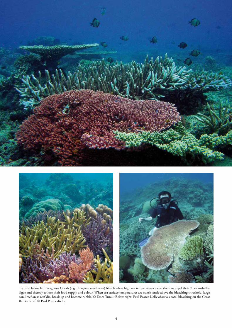
Top and below left: Staghorn Corals (e.g., Acropora cervicornis) bleach when high sea temperatures cause them to expel their Zooxanthellae algae and thereby to lose their food supply and colour. When sea surface temperatures are consistently above the bleaching threshold, large coral reef areas reef die, break up and become rubble. © Emre Turak. Below right: Paul Pearce-Kelly observes coral bleaching on the Great Barrier Reef. © Paul Pearce-Kelly

5

2.1Definitionsofcommonlyusedterms

Climate Change The IPCC’s most recent (fifth) assessment report defines climate change as “a change in the state of the climate that can be identified (e.g., by using statistical tests) by changes in the mean and/or the variability of its properties, and that persists for an extended period, typically decades or longer” (IPCC, 2013a). Climate change results from both natural global cycles as well as from external drivers of change such as shifts in solar cycles, volcanic eruptions and persistent human influences on the composition of the atmosphere or land cover. In both the scientific literature and a wider global context, the term is commonly used to describe the changes that are attributable solely or predominantly to human activities. These may be at local, regional and global scales and are widely regarded as having begun at the onset of the Industrial Revolution in the 18th century.

We note that the GCM community strongly advocates using the term “scenario” rather than “prediction” to refer to model outcomes based on emissions pathways. Essentially, the difference is that scenarios use an explicit “if… then…” whereas we often forget the “if…” part when using the term “prediction”. The distinction is semantic, but it addresses the

highly likely possibility that the world will not evolve exactly as our models indicate it could, even if socioeconomic conditions were to conform exactly to those for any particular emissions scenario. Given the many uncertainties inherent in CCVAs, they should be regarded as scenario-based.

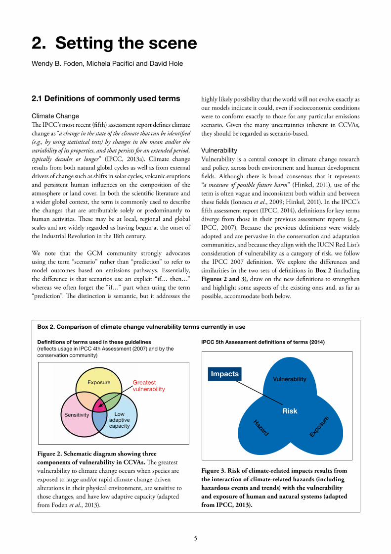
VulnerabilityVulnerability is a central concept in climate change research and policy, across both environment and human development fields. Although there is broad consensus that it represents “a measure of possible future harm” (Hinkel, 2011), use of the term is often vague and inconsistent both within and between these fields (Ionescu et al., 2009; Hinkel, 2011). In the IPCC’s fifth assessment report (IPCC, 2014), definitions for key terms diverge from those in their previous assessment reports (e.g., IPCC, 2007). Because the previous definitions were widely adopted and are pervasive in the conservation and adaptation communities, and because they align with the IUCN Red List’s consideration of vulnerability as a category of risk, we follow the IPCC 2007 definition. We explore the differences and similarities in the two sets of definitions in Box 2 (including Figures 2 and 3), draw on the new definitions to strengthen and highlight some aspects of the existing ones and, as far as possible, accommodate both below.

2. SettingthesceneWendy B. Foden, Michela Pacifici and David Hole

IPCC5thAssessmentdefinitionsofterms(2014)

Box2.Comparisonofclimatechangevulnerabilitytermscurrentlyinuse

Definitionsoftermsusedintheseguidelines(reflects usage in IPCC 4th Assessment (2007) and by the conservation community)

Figure 2. Schematic diagram showing three components of vulnerability in CCVAs. The greatest vulnerability to climate change occurs when species are exposed to large and/or rapid climate change-driven alterations in their physical environment, are sensitive to those changes, and have low adaptive capacity (adapted from Foden et al., 2013).

Figure 3. Risk of climate-related impacts results from the interaction of climate-related hazards (including hazardous events and trends) with the vulnerability and exposure of human and natural systems (adapted from IPCC, 2013).

Vulnerability

Hazard Exposure

Risk

ImpactsGreatest vulnerability

Exposure

Sensitivity Low adaptive capacity

6

IUCN SSC Guidelines for Assessing Species’ Vulnerability to Climate Change

Overarchingmeasuresofconcern

VulnerabilityThe extent to which biodiversity is susceptible to or unable to cope with the adverse effects of climate change. It is a function of the character, magnitude and rate of climate change to which the system is exposed, its sensitivity and its adaptivecapacity (IPCC, 2007a) (Differs from IPCC, 2014).

RiskThe probability of harmful consequences resulting from climate change. Risk results from the interaction of vulnerability, exposure, and hazard. Risk is often represented as probability of occurrence of hazardous events or trends multiplied by the impacts if these events or trends occur (IPCC, 2014) (not defined in 2007).

ImpactThe effects, consequences or outcomes of climate change on natural and human systems. It is a function of the interactions between climate changes or hazardous climate events occurring within a specific time period and the vulnerability of an exposed society or system (IPCC, 2014). (Differs from IPCC, 2007, which describes impacts as potential or residual based on adaptation potential).

Intrinsiccontributingfactors

SensitivitySensitivity is the degree to which a system is affected, either adversely or beneficially, by climate variability or change (IPCC, 2007a, 2014).

AdaptiveCapacityThe potential, capability, or ability of a species, ecosystem or human system to adjust to climate change, to moderate potential damage, to take advantage of opportunities, or to respond to the consequences (IPCC, 2007a, 2014).

Vulnerability‘The propensity or predisposition to be adversely affected. In this usage, vulnerability encompasses a variety of concepts, particularly sensitivity to harm and lackofcapacitytocopeandadapt.’ (IPCC, 2014) (Differs from IPCC, 2007).

ExposureThe presence of people, livelihoods, species or ecosystems, environmental functions, services, and resources, infrastructure, or economic, social, or cultural assets in places and settings that could be adversely affected (IPCC, 2014) (Not defined in IPCC, 2007).

Externalcontributingfactors

ExposureExposure describes the nature, magnitude and rate of climatic and associated environmental changes experienced by a species (Dawson et al., 2011; Foden et al., 2013; Stein et al., 2014) (Not defined in IPCC, 2007).

HazardThe potential occurrence of a natural or human-induced physical event or trend or physical impact that may cause loss of life, injury, or other health impacts, as well as damage and loss to property, infrastructure, livelihoods, service provision, ecosystems, and environmental resources. In this report, the term hazard usually refers to climate-related physical events or trends or their physical impacts (IPCC, 2014) (Not defined in IPCC, 2007).

We consider climate change vulnerability to be the extent to which biodiversity will be adversely affected by climate change (IPCC 2007; IPCC, 2014). This description is useful for general and conceptual purposes; when users begin making use of the term for more specific purposes such as for assessments of climate change vulnerability, definition of key vulnerability variables is required (see Figure 2). Climate change vulnerability may describe a range of different biological hierarchy levels or entities (e.g., from subpopulations to ecosystems), at different spatial scales (e.g., from sites to globally), considering different biodiversity impact types (e.g., from extinction risk to declines in ecosystem function or evolutionary diversity), considering different aspects of climate change (e.g., impacts from direct climate change to indirect impacts from humans

and biodiversity responding to climate change) and covering considerably different time frames (e.g., 5 year to 100 year time frames). Many studies have failed to explicitly define such variables, resulting in difficulties with interpreting and comparing among results. In the context of climate change vulnerability assessment, we strongly encourage users of the term “climate change vulnerability” to explicitly define their key variables, namely the ‘Entity (OF)’, ‘Spatial scale’ (IN), ‘Impact type’ (TO), ‘Cause’ (FROM) and ‘Time frame’ (WITHIN), in which vulnerability is being considered (Figure 4).

Vulnerability is a function of the character, magnitude and rate of the climate change to which the species or entity is exposed (i.e., external factors), and its intrinsic sensitivity and adaptive

7

capacity. These three components of vulnerability, namely exposure, sensitivity, and adaptive capacity, provide a valuable entry point into climate change vulnerability assessments. While these terms can be broadly applied at a range of scales to both natural and human systems, we outline them below in the context of species’ vulnerability to climate change and highlight their relationship with climate change vulnerability in Figure 2.

ExposureExposure describes the nature, magnitude and rate of changes experienced by a species, and includes changes in both direct climatic variables (e.g., temperature, precipitation) and associated factors (e.g., sea level rise, drought frequency, and ocean acidification) (e.g., Stein et al., 2014). Changes in habitats and regions occupied by the species are also included (e.g., Dawson et al., 2011). Measures of future climate exposure are typically informed by scenario projections derived from General Circulation Models (GCMs).

SensitivitySensitivity is the degree to which a species, habitat or ecosystem is or is likely to be affected by or responsive to changes (e.g., Glick et al., 2011). This depends on how tightly the species is

coupled to its historical climatic conditions, particularly those climate variables that are expected to change in the future (e.g., Dawson et al., 2011).

Sensitivity is mediated by a range of characteristics that influence the fitness of individuals and recovery of populations comprizing a species. These characteristics include physiological, behavioural and life history traits that influence: the degree to which species are buffered from exposure to sub-optimal conditions; their ability to tolerate changes in environmental conditions and cues, as well as in interspecific interactions; and their ability to regenerate and recover following impacts. The characteristics also include within and across-generation plastic responses and genetic variability in traits that facilitate regeneration and recovery.

Adaptive capacityAdaptive capacity describes the degree to which a species, habitat or ecosystem is able to reduce or avoid the adverse effects of climate change through dispersal to and colonization of more climatically suitable areas, plastic ecological responses, and/or evolutionary responses (Williams et al., 2008; Nicotra et al., 2015; Beever et al., 2016).

Figure 4. Five key parameters for describing vulnerability of biodiversity to climate change. An example of a specific use for assessing an ecosystem is: “Vulnerability OF temperate forests IN North America TO declines in carbon storage FROM temperature and precipitation changes and pine bark beetle damage WITHIN the next 50 years”. An example of specific use for assessing species is: “Vulnerability OF tuna species IN the southern Atlantic TO range shifts and population declines FROM rising ocean temperatures WITHIN the next 10 years”.

ULNERABILITY

Fig 4

2. Setting the scene

8

IUCN SSC Guidelines for Assessing Species’ Vulnerability to Climate Change

HazardThe magnitude of a natural or human-induced climate-related physical event or change that may cause impacts on species.

ImpactThe expected or observed loss or gain in species, habitat or ecosystems due to a hazardous event.

RiskThe potential consequences to species of future climate change. Risk is often represented as probability of occurrence of hazardous events or trends multiplied by the impacts if these events or trends were to occur.

2.2 Climatechangevulnerabilityassessmentapproaches

Here we discuss the approaches commonly used to carry out CCVAs. Understanding the origins, principles, advantages and limitations of these approaches is important both for those needing to select approaches and the methods used to apply them, as well as those wishing to use CCVA outputs that others have generated. The methods used to date to assess species’ CCVA can be classified into three main approaches: 1) correlative; 2) mechanistic; and 3) trait-based. These approaches are summarized in Figure 5, based on a review carried out by Pacifici et al. (2015), which should be referred to for further details and examples. The figure includes examples of the application of each approach, as well as combinations of more than one approach.

2.2.1Correlativeapproaches

The use of correlative models, also referred to as niche-based or species distribution models, for climate change vulnerability assessment began around the early 1990s (e.g., Busby, 1991; Walker & Cocks, 1991; Carpenter et al., 1993). They use correlations between each species’ distribution ranges and its historical climate to estimate its climatic requirements, or climatic niche (e.g., Hutchinson, 1957). Using this information and projections of future climates, these models predict the potential geographic areas of suitable climate for the species in the future (e.g., Pearson & Dawson, 2003; Beale et al., 2008). Consideration of whether species will be able to disperse to and colonize such areas, as well as whether biotic and abiotic conditions are suitable for them, are important when interpreting whether areas predicted to be of potentially suitable future climate could become part of species’ future distribution ranges. Species’ climate change vulnerability is typically inferred from predicted difference in range size and location, and occasionally from changes in degree of fragmentation (e.g., Garcia et al., 2014b).

Correlative models’ assumption that species’ distributions are in equilibrium with their climates is problematic, since

this ignores the roles that inter-specific interactions, habitats, geographic barriers and humans play in shaping current distributions (Guisan & Thuiller, 2005). Correlative approaches perform poorly for narrowly-distributed species (which are typically those most threatened and of greatest conservation concern) both because their distributions are less likely to be constrained by climate pressures, and because the models’ statistical requirements for many spatially independent occurrence records cannot be met (e.g., Stockwell & Peterson, 2002; Platts et al., 2014). Correlative methods typically ignore the many mechanisms of climate change impacts beyond shifting climatic suitability (e.g., loss of resource or mutualist species) that have been shown to be important causes of climate-change related population declines (e.g., Ockendon et al., 2014). In addition, they do not consider the biological traits that are known to play an important role in shaping species’ sensitivity and adaptive capacity to climate change (e.g., Jiguet et al., 2007; Dawson et al., 2011). Further discussion on the caveats and limitations of correlative approaches is found in Heikkinen et al. (2006), Araújo et al. (2012) and Franklin (2013).

Despite these drawbacks, correlative methods have been shown to perform well in predicting observed climate change-driven range shifts (e.g., Chen et al., 2011; Dobrowski et al., 2011; Morelli et al., 2012; Smith et al., 2013) and changes in

Figure 5. Summary of the three main CCVA approaches (1–3) and the six categories their combinations create, as well as published examples of their use.

1.Correlative: e.g.,Thuilleret al.,2005;Huntleyet al.,2008a;Araújoet al.,2011

2.Trait-based:e.g.,Chinet al.,2010;Younget al.,2011;Fodenet al.,2013

3.Mechanistic:e.g.,Kearney&Porter,2009;Monahan,20094.Correlative-Trait-based:e.g.,Schlosset al.,2012;Warrenet al.,

2013;Garciaet al.,2014a5.Correlative-Mechanistic:e.g.,Andersonet al.,2009;Midgleyet

al.,2010;Aiello-Lammenset al.,2011;Lauranceet al.,20126. Correlative-Trait-Mechanistic:e.g.,Thomaset al.,2011;Keith

et al.,2014

1Correlative

3Mechanistic

2Trait-based

4

6

5

9

population abundance (e.g., Gregory et al., 2009). They do not require information on species biology as input data, and they deliver spatially explicit outputs that are informative for spatial conservation planning (e.g., Hannah et al., 2002; Araújo et al., 2004; Phillips et al., 2008; Araújo et al., 2011). Tools with user-friendly interfaces such as MaxEnt (e.g., Phillips et al., 2004; Phillips & Dudı, 2008), BIOMOD (e.g., Thuiller, 2003) and the Wallace Initiative (e.g., Warren et al., 2013) are available to apply several correlative methods. They can also be applied to assess impacts of climate change on species across networks of sites identified for conserving particular species, such as protected areas or Key Biodiversity Areas, by projecting species distribution models onto individual climates for each site in a network (e.g., Hole et al., 2009; Bagchi et al., 2013). Appendix Table A provides a summary of the types of correlative methods available for CCVA, examples of their use, as well as the tools available for their application. Pearson (2007) provides an excellent and accessible reference for understanding and using correlative methods, including for CCVA.

2.2.2Trait-basedapproaches

Trait-based vulnerability assessment approaches (TVAs) use species’ biological characteristics to estimate their sensitivity and adaptive capacity to climate change, typically combining these with estimates of the extent of their exposure to climate changes (e.g., Williams et al. 2008, Young et al. 2012, Foden et al. 2013a, Smith et al. 2016). These methods require biological data and typically also broad-scale distribution information (e.g., a distribution range map). Biological knowledge of the focal taxonomic group is required to parameterize how, and to what extent, individual traits relate to climate change vulnerability, as well as to evaluate each species according to their possession of these traits. Exposure may be estimated using GIS-based modelling (e.g., Foden et al., 2013), user-friendly interfaces presenting generalized climate projections (e.g., http://www.climatewizard.org/), any number of statistical programs or languages (e.g., R, Python, MatLAB), or expert judgment (e.g., Chin et al., 2010). Where species’ distribution information is lacking or where simplistic or preliminary assessments alone are required, exposure assessments are sometimes omitted (e.g., McNamara, 2010; Advani, 2014). Sensitivity, adaptive capacity and preferably exposure scores are then combined to assign species to a category of vulnerability. Appendix Table B provides a summary of the types of trait-based methods available for CCVA, examples of their use, as well as the tools available for their application.

Trait-based approaches are most widely used to inform prioritization of species for conservation interventions. Because they are unable to predict species’ suitable future climate space, they provide more limited support for spatial conservation planning. Further, the precise vulnerability thresholds associated with each trait are seldom known, requiring estimation or selection of arbitrary relative values (e.g., Foden et al., 2013; Garcia et al., 2014a). There is little consensus

on approaches for combining trait scores to assess exposure, sensitivity or adaptive capacity scores, nor for combining these into overall CCVA scores, and many methods simply weight traits equally (e.g., Laidre et al., 2008; Foden et al., 2013) even though some characteristics are likely to be more important than others in determining climate change vulnerability (e.g., Pacifici et al., 2015). Because many traits tend to be taxon-group specific, most methods don’t allow direct comparison of vulnerability among taxonomic groups.

Although TVAs were amongst the earliest proposed approaches (e.g., Herman & Scott, 1994), they have only gained prominence recently (e.g., Williams et al., 2008; Graham et al., 2011; Young et al., 2015) and hence remain largely unvalidated. They are becoming increasingly used by conservation organizations and management agencies, however (e.g., Bagne et al., 2011; Glick et al., 2011; Carr et al., 2013; Foden et al., 2013; Johnson, 2014; Young et al., 2015; Hare et al., 2016), since they allow relatively rapid vulnerability assessment for multiple species, do not necessarily require modelling expertise (e.g., Pacifici et al., 2015), and because their involvement of experts and easily understood and applied methods promote buy-in and use. They allow consideration of many mechanisms of climate change impacts on species, and their consideration of species’ biological traits meets the growing recognition of the need to consider species’ individualistic responses to climate change. Finally, they are applicable to all species, irrespective of their distribution size; this and their relatively low requirements for detailed distribution information mean that they can be widely applied to all members of entire taxonomic groups, making them particularly useful for broad-scale conservation assessments.

2.2.3Mechanisticapproaches

Mechanistic or process-based models predict species’ likely responses to changing environmental conditions by explicitly incorporating known biological processes, thresholds and

David Bickford with a Fordonia Mangrove Snake (Fordonia leucobalia). This species is found almost exclusively in mangroves, which are vulnerable to inundation when sea levels rise faster than they are able to cope with. Countless other species will also be affected. © David Bickford

2. Setting the scene

10

IUCN SSC Guidelines for Assessing Species’ Vulnerability to Climate Change

interactions (e.g., Morin & Thuiller, 2009). Mechanistic niche models use estimates of species’ physiological tolerances, typically from laboratory and field observations (e.g., Jenouvrier et al., 2009; Radchuk et al., 2013; Overgaard et al., 2014) or from energy balance equations (e.g., Molnár et al., 2010; Huey et al., 2012), to estimate niche parameters. This provides an approximation of species’ potential or fundamental niche, thereby avoiding the limitation faced by correlational approaches due to their assumption that species are at equilibrium with their environments.

Mechanistic models are able to accommodate a broad range of climate change impact mechanisms including changes in resource availability (e.g., Hoffmann et al., 2010), land use (e.g., Mantyka-Pringle et al., 2014; Martin et al., 2015), predation, competition (e.g., Urban et al., 2012), stream flow (e.g., Crozier et al., 2008) and changes in habitat suitability (e.g., Hunter et al., 2010; Aiello-Lammens et al., 2011; Forrest et al., 2012). They can include species-specific characteristics such as dispersal distances (e.g., Kearney et al., 2008; Keith et al., 2008), longevity, fecundity (e.g., Saltz et al., 2006), density dependence (e.g., Leroux et al., 2013), morphological factors, genetic evolution, phenotypic plasticity (e.g., Chevin et al., 2010; Huey et al., 2012) and demographic stochasticity (e.g., Hunter et al., 2010). They can also include interactions between mechanisms such as land use change and climate change (Mantyka-Pringle et al., 2014, 2016). Other mechanistic models consider the changes in vegetation distribution and dynamics using groups of species (e.g., plant functional types), based on bioclimatic and physiological parameters (e.g., Morin & Thuiller, 2009). Appendix Table C provides a summary of the types of mechanistic methods available for CCVA, examples of their use, as well as the tools available for their application.

Key strengths of mechanistic models include their ability to inform a mechanistic understanding of the processes driving climate change vulnerability (Kearney & Porter, 2009), provide a credible way to forecast response to novel situations (e.g. extrapolate rather than interpolate) and form the basis for identifying responses implications for management actions (e.g., Fordham et al., 2013a; Mantyka-Pringle et al., 2016). They include a range of climate change impact mechanisms, consider species’ individual biological traits and may be applied to narrowly distributed species. However, their generally intensive requirements for physiological, demographic and distribution knowledge and data (Morin & Thuiller, 2009), and hence their relative costliness (Kearney & Porter, 2009; Chevin et al., 2010), is a significant limiting factor in their application which, to date, is restricted to only a few well-studied species.

2.2.4Combinedapproaches

The approaches discussed above are those most commonly used in vulnerability assessments. However, there is a growing consensus that combining approaches may yield models that capture the advantages of each. Here we briefly discuss

combinations of the approaches that have been applied to date, noting that, to our knowledge, no studies of combined trait-based and mechanistic approaches have been published. Appendix Table D provides a summary of the types of combination approach methods available for CCVA, examples of their use, as well as the tools available for their application.

Correlative-TVA approachesCorrelative and trait-based approaches are typically combined in two ways. In the first, traits are used to create more biologically realistic correlative models, and data such as dispersal distances, generation lengths and habitat preferences are used to refine estimates of species’ exposure and/or range dynamics. Schloss et al., (2012), for example, used natal dispersal and generation length to predict the future distribution of terrestrial mammals in the Western Hemisphere under climate and land-use changes, and Warren et al., (2013) have applied a similar approach to a range of taxonomic groups. Prevalence of certain traits has also been used to identify species and regions where correlative models may under- or over-predict climate change vulnerability (e.g., Garcia et al., 2014a). In the second approach, correlative model results may be included in trait-based approaches to contribute to overall measures of vulnerability (e.g., Young et al., 2012). By integrating exposure calculated with correlative models, the indices derived from TVAs acquire more reliable estimates of the risks posed by climate change, accounting for both intrinsic and extrinsic factors (Willis et al., 2015).

Correlative-Mechanistic approachesOutputs of correlative models may be used to project the location of a species’ suitable climate space in various time steps into the future, while mechanistic models project resulting impacts on habitat suitability and population dynamics resulting from these changes across landscapes (Keith et al., 2008; Anderson et al., 2009; Midgley et al., 2010; Aiello-Lammens et al., 2011). Some studies have integrated life-history characteristics into models to produce more accurate projections of species’ responses to climate change (e.g., Midgley et al., 2010) while others have additionally included inter-species interactions (e.g., Harris et al., 2012; Fordham et al., 2013).

Criterion-based methods: a combined Correlative-Mechanistic-Trait approachThomas et al. (2010) used combinations of species’ observed changes (e.g., recorded population declines), projected changes (potentially from correlative and/or mechanistic models) and life history traits (e.g., generation length) to estimate climate change vulnerability of a range of UK species. Similar to the IUCN Red List, the various information sources were combined through a criterion-based system that classified species into vulnerability categories based on quantitative thresholds. Such criterion-based methods can account for several factors known to affect species’ relative extinction risk (e.g., decline in extent of occurrence, reduction in population size), and are able to accommodate species for which different amounts of data are available.

11

Criteria that predict vulnerability to climate change can overlap extensively with those used in IUCN Red List assessments. Pearson et al. (2014) found that characteristics predisposing a selection of North American herpetofauna to climate change vulnerability are also included in the information already compiled to assess species’ extinction risk through the IUCN Red List categories and criteria. In related studies, Pearson et al. (2014), Stanton et al. (2015) and Keith et al. (2014) showed that IUCN Red List extinction risk category is a good predictor of climate change vulnerability for six groups of North American reptiles and salamanders, and for an Australian frog species. Akçakaya et al., (2014) concluded that these studies suggest that IUCN Red List assessments, if sufficiently frequently updated, reflect extinction risk owing to climate change vulnerability, and can provide decades of warning time before species go extinct. Further research is needed to extend the approach to other taxonomic groups. For IUCN Red List assessments to give results comparable across taxonomic groups, it is essential that the thresholds and time periods used in the criteria are not altered (Akçakaya et al., 2006), and the guidelines developed by IUCN are followed (IUCN Standards and Petitions Subcommittee, 2014).

2.3 Metricsforestimatingclimatechangevulnerability

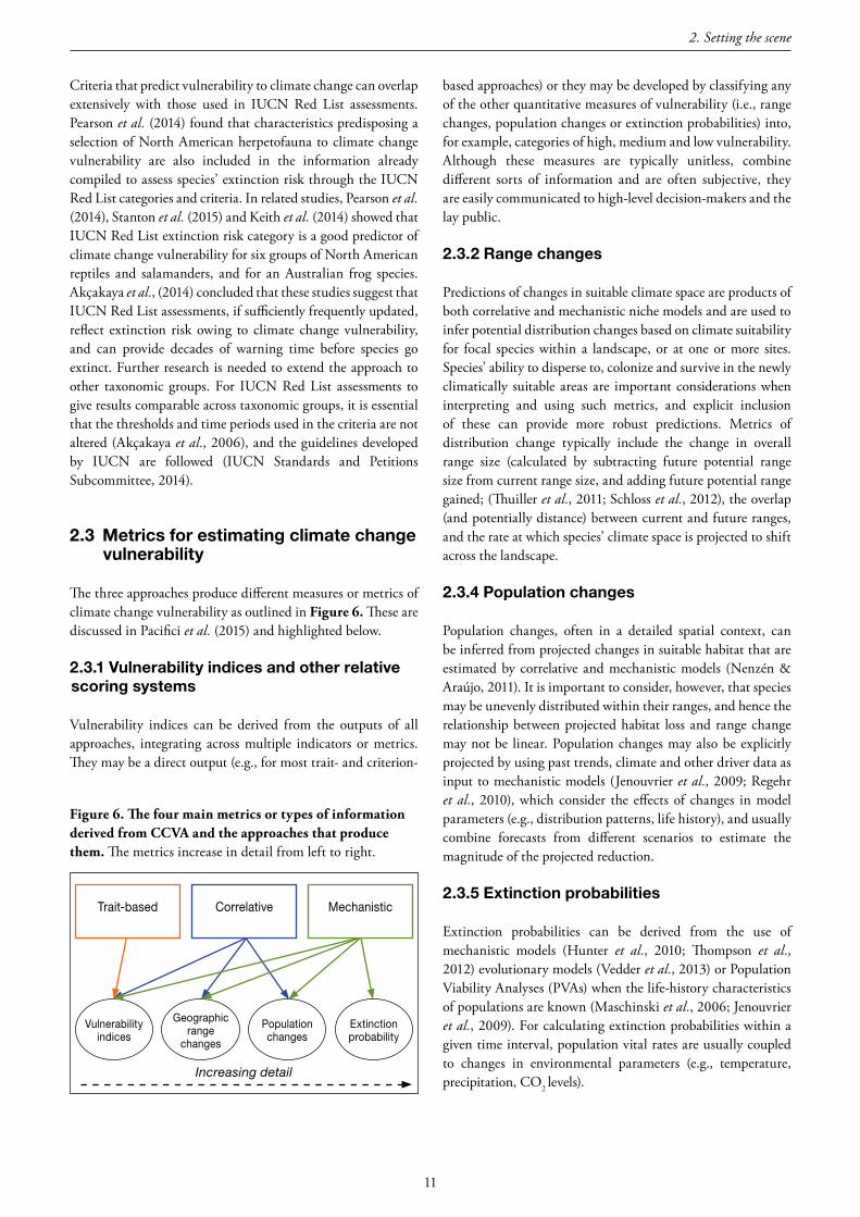
The three approaches produce different measures or metrics of climate change vulnerability as outlined in Figure 6. These are discussed in Pacifici et al. (2015) and highlighted below.

2.3.1Vulnerabilityindicesandotherrelativescoringsystems

Vulnerability indices can be derived from the outputs of all approaches, integrating across multiple indicators or metrics. They may be a direct output (e.g., for most trait- and criterion-

based approaches) or they may be developed by classifying any of the other quantitative measures of vulnerability (i.e., range changes, population changes or extinction probabilities) into, for example, categories of high, medium and low vulnerability. Although these measures are typically unitless, combine different sorts of information and are often subjective, they are easily communicated to high-level decision-makers and the lay public.

2.3.2Rangechanges

Predictions of changes in suitable climate space are products of both correlative and mechanistic niche models and are used to infer potential distribution changes based on climate suitability for focal species within a landscape, or at one or more sites. Species’ ability to disperse to, colonize and survive in the newly climatically suitable areas are important considerations when interpreting and using such metrics, and explicit inclusion of these can provide more robust predictions. Metrics of distribution change typically include the change in overall range size (calculated by subtracting future potential range size from current range size, and adding future potential range gained; (Thuiller et al., 2011; Schloss et al., 2012), the overlap (and potentially distance) between current and future ranges, and the rate at which species’ climate space is projected to shift across the landscape.

2.3.4Populationchanges

Population changes, often in a detailed spatial context, can be inferred from projected changes in suitable habitat that are estimated by correlative and mechanistic models (Nenzén & Araújo, 2011). It is important to consider, however, that species may be unevenly distributed within their ranges, and hence the relationship between projected habitat loss and range change may not be linear. Population changes may also be explicitly projected by using past trends, climate and other driver data as input to mechanistic models (Jenouvrier et al., 2009; Regehr et al., 2010), which consider the effects of changes in model parameters (e.g., distribution patterns, life history), and usually combine forecasts from different scenarios to estimate the magnitude of the projected reduction.

2.3.5Extinctionprobabilities

Extinction probabilities can be derived from the use of mechanistic models (Hunter et al., 2010; Thompson et al., 2012) evolutionary models (Vedder et al., 2013) or Population Viability Analyses (PVAs) when the life-history characteristics of populations are known (Maschinski et al., 2006; Jenouvrier et al., 2009). For calculating extinction probabilities within a given time interval, population vital rates are usually coupled to changes in environmental parameters (e.g., temperature, precipitation, CO2 levels).

Figure 6. The four main metrics or types of information derived from CCVA and the approaches that produce them. The metrics increase in detail from left to right.

Increasing detail

Vulnerabilityindices

Geographicrange

changes

Populationchanges

Extinction probability

Trait-based Correlative

2. Setting the scene

Mechanistic

12

IUCN SSC Guidelines for Assessing Species’ Vulnerability to Climate Change

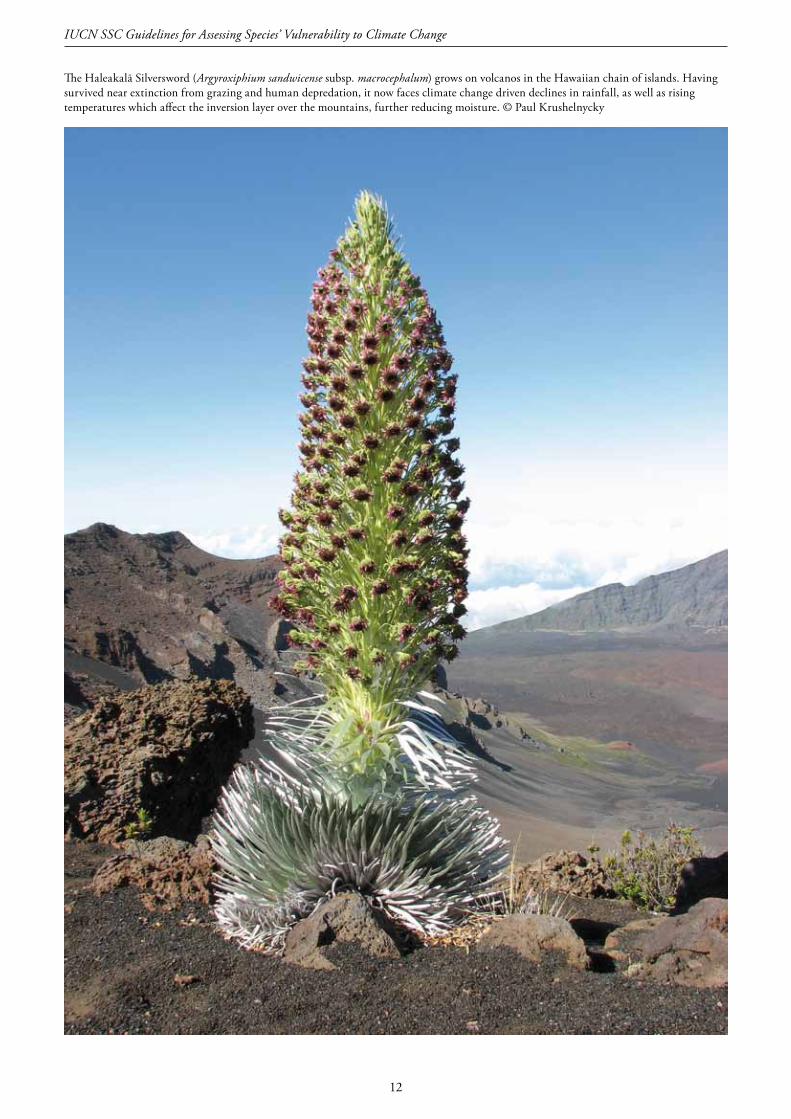
The Haleakalā Silversword (Argyroxiphium sandwicense subsp. macrocephalum) grows on volcanos in the Hawaiian chain of islands. Having survived near extinction from grazing and human depredation, it now faces climate change driven declines in rainfall, as well as rising temperatures which affect the inversion layer over the mountains, further reducing moisture. © Paul Krushelnycky

13

3.1 Definingyourgoal

Clear goals facilitate the establishment of well-structured objectives and promote clear, verifiable CCVA outputs and effective conservation impacts. Being clear about the needed outcomes before initiating research will help ensure: i) that the outputs of the analysis will fulfil needs; ii) that assessments will not need to be repeated soon; iii) that the project can be completed in a reasonable amount of time without cost overruns; and iv) that the results will influence the intended audience. We reiterate the importance, when setting goals, of distinguishing between CCVA (which this document describes) and adaptation planning (which is not this document’s focus). Climate change vulnerability assessments are carried out to help identify what is at risk and why, while climate change adaptation planning, which is informed by CCVA information, focuses on how to respond to these risks.

A well-defined goal answers the following questions: 1. Why are you carrying out this CCVA?2. Who is your audience?3. Which decisions do you hope to influence using the results?

3.1.1WhyareyoucarryingoutthisCCVA?

Start by answering this basic question. Knowing in a general sense the achievements anticipated by the vulnerability assessment will then guide answers to other questions about the audience addressed and the decisions to be influenced, as well as the specific objectives that will further define the project. Examples of goals you may have for your CCVA are:• To determine the degree of vulnerability to climate change

of one or more species in a particular region or across their entire ranges.

• To perform an academic exercise.• To provide input into a specific adaptation planning process

(designed to address a single species, a suite of species, a geographic area, or something else) that is either underway or planned.

• To obtain quantitative information about a species’ response to a changing climate as input into a demographic model.

• To use a vulnerability assessment as a means to learn more about how climate change might influence species of interest to a particular group of people.

Regardless, answering this basic “why” question will help address the subsequent questions, which in turn will guide you in choosing an appropriate methodology for your assessment.

3.1.2Whoisyouraudience?

Vulnerability assessments may be targeted at one or more audiences, including policymakers, land/resource managers, scientists or the general public. Audiences can vary widely in their objectives, as well as in their management and decision-making processes, and these differences can affect the specifics of the vulnerability assessment, including the choice of methods, level of needed rigor, the reporting styles and the objectives of the assessment itself. For example, language used to address the public will be less technical than that used to address the scientific community. Similarly, resource managers and policymakers will require information to be communicated in a language that is directly relevant to the contexts (e.g., biological, legislative) in which they work.

3.1.3Whichdecisionsdoyouhopetoinfluenceusingtheresults?

Understanding how the audience for an assessment engages in planning and management processes is key to developing the objectives of a vulnerability assessment. The results of an assessment are more likely to have an impact if they align with the management needs of the intended audience. For example, at the local level, managers might develop site conservation plans for the planning, implementation and monitoring of management actions at a single site. By contrast, government entities such as a national parks agency may develop management plans for a network of sites. A subnational government may be interested in prioritizing species that occur within their jurisdiction for management consideration. In each situation, the management process is different and requires vulnerability assessments with different objectives.

3.2 Definingyourobjectives

Objectives describe the one or more specific action steps needed to achieve your CCVA goal. We describe six broad CCVA objective categories.

To identify, for specified taxonomic groups, regions AND time frames:• Which species are most vulnerable• Howmuch–howvulnerable species are (i.e., the magnitude

of vulnerability)• Why species are vulnerable• Where species are vulnerable

3.SettingClimateChangeVulnerabilityAssessmentgoalsandobjectivesBruce E. Young, Tara Martin, James Watson, Wendy B. Foden, Stephen Williams and Brett Scheffers

14

IUCN SSC Guidelines for Assessing Species’ Vulnerability to Climate Change

• When species become vulnerable• What’smissing (i.e., what data and information are needed

to be able to carry out a good CCVA).

Scale is a fundamental consideration in ecological and conservation science (Levin, 1992). Patterns exist at multiple levels of organization across a wide range of taxonomic, spatial and temporal scales. Identifying appropriate scales of focus for a given CCVA and defining objectives in terms of each are critically important steps in setting clear, effective objectives since they will directly influence the approaches, methods and resources required to address them.

3.2.1Selectingataxonomicfocus

CCVAs can be carried out at species, subspecies, metapopulation, population or individual levels, as well as at higher taxonomic levels (e.g., genera) or for species from multiple taxonomic groups (e.g., all vertebrate species occurring in a particular area or belonging to a specific functional group or guild). Most assessments, however, focus at the species level or below since these entities tend to (though do not always) have relatively consistent biological characteristics (e.g., climatic tolerances and dispersal abilities). We encourage users, as far as possible, to make use of widely accepted taxonomic classification systems (e.g., see the IUCN Red List taxonomic standards and references1) in order to maximize applicability and comparability of outputs.

A checklist is provided below to assist practitioners in setting clearly defined objectives (Table 1). Examples of objectives, grouped according to their taxonomic focus, spatial extent and objective categories, are shown in Table 2.

3.2.2Selectingaspatialfocus

An assessment’s spatial focus may be a taxon’s range (e.g., the entire distribution of a species, subspecies or subpopulation), a site (e.g., an individual protected area or discrete area containing a subpopulation of a species, such as a Key Biodiversity Area) or a network of such sites, a political or administrative unit such as a state or nation, or a larger spatial scale (including a land- or sea-scape, region, continent or even the world). Some CCVA approaches and methods have specific requirements for setting spatial foci, so a more detailed discussion of selection of CCVA focal extent is included in Section 5.1.1 (Spatial extent and resolution).

3.2.3Selectingatimeframe

Time frames of assessments are most often shaped by users’ specific interests or needs (e.g., a 10-year planning horizon for site manager) in conjunction with the following important considerations. For taxon-focused assessments, species’

1 http://www.iucnredlist.org/technical-documents/information-sources-and-quality#standards

generation lengths should be an important consideration. For shorter-lived species, shorter projection intervals are more appropriate (e.g., as per the IUCN Red List guidelines, three generations, but with a minimum of 10 years), while for longer-lived species, longer projection intervals are needed to adequately consider vulnerability (e.g., three generations, but to a maximum of 100 years).

Uncertainty in climate projections is considerably higher further into the future, so the range of plausible results increases over very long time frames (e.g., >50 years). However, confidence in projecting whether a species is vulnerable is most likely going to increase with time for many species. Because projections are calculated as means, those for shorter time periods (e.g., <20 years) are more prone to bias by extreme values. In the IPCC’s latest (2013) projections, for example, 20-year intervals are reflected, namely 2016–35 (2025 mean), 2046–65 (2055 mean) and 2081–2100 (2090 mean). While obtaining detailed model output and compiling projections for custom periods is possible, this requires considerable processing and appropriate expertise. Using the readily available means does, however, limit the time frames that can be considered when computing the CCVA.

Table 1. Checklisttoaididentificationofclear,quantitativeobjects.

i)Selectanobjectivecategory:

Which? Howmuch?

Why? Where? When? What’smissing?

ii) Selectataxonomicfocus(forexample):

Population Species Onetaxonomicgroup

Multipletaxonomicgroups

Selectaspatialfocus:

iii) Taxon’srange Site Networkofsites

Largerspatialscales

iv)Selectatimeframe(forexample):

100years 50years 20years 5years Present

A Rhacophorus angulorostris frog from Mt. Kinabalu, Borneo. These frogs require clean, fast-flowing montane rivers to breed so any disruption to typical seasonal rainfall can have pronounced effects on reproductive success. Conditions on the mountains are becoming drier and hotter and a protracted drought could spell disaster for this and many other amphibian species. © David Bickford

15

Table 2.HeuristicexamplesofCCVAobjectives,groupedaccordingtosixobjectivecategories,andtheirscopeoffocus.

Examples of CCVA objectives.To identify, forspecifiedtaxonomicgroups,regionsandtimeframes:

Taxonomicfocus

Which? • Whichspecies(e.g.,birds,amphibians,plants)aremostandleastvulnerabletoclimatechangeacrosstheirglobaldistributionranges

• Whichoftheorganisms(e.g.,marinefishes,rainforestseed-dispersers,migratoryanimals)aremostandleastvulnerabletoclimatechange

• Whichpopulationofathreatenedspeciesismostandleastclimatechangevulnerable

Howmuch? • Howmuchisthefocalspecies’suitableclimatespacelikelytocontractorexpandoverthenext10/25/50/100years• Howfarandfastwillthespeciesneedtomovetotracktheirclimatespaceby2050

Why? • Whichimpactmechanismswillthespeciesface• Isthespeciessensitive,exposedand/orpoorlyadaptivetodirect/indirectclimatechange• Whichcomponentsofthechangingclimateposethegreatestrisktothefocalspecies(e.g.,maximumtemperaturesvs.water

availabilityinthedryseason,increaseddiscreteeventsvs.long-termcontinuousevents)

Where? • Whichareaswillbeclimaticallysuitableforthefocalspeciesin10/25/50years’time• Whichregionsorcountriescontainspeciesmostvulnerabletoclimatechange• Whetherthemostclimatechangevulnerablespeciesoccurinareaswherehumansarealsomostvulnerabletoclimatechange

When? • Whetherclimatechangeislikelytoaffectthespecieswithinthenext10years• Whentheclimatewithinaspecificsectionofthespecies’rangewillnolongerbesuitable

What’smissing?

• Whicharethekeyuncertaintiesthatrequireadditionaldatacollectionand/orresearchforbetterassessingvulnerabilitytoclimatechangeofthespecies

Spatialfocusonmultiplespeciesatasingle site

Which? • Whichspeciescurrentlyoccurringinaprotectedareaaremostandleastvulnerabletoclimatechange• Forwhichcurrentlyoccurringspeciesthesitewillremainorbecomeclimaticallysuitablein10/25/50years’time• Forwhichspeciesnotcurrentlyoccurringatthesiteitmaybecomesuitablein10/25/50years’time

Howmuch? • Whatisthepredictedturnover(i.e.,lossandgain)ofspeciesatthesiteby2050

Why? • Whichaspectsofvulnerability(i.e.,sensitivity,exposureand/orpooradaptivecapacity)aremostprevalentforthespeciesatthesite

• Whichaspectsofprojectedclimatechangeplaythegreatestroleindrivingclimatechangeriskforspeciesatthesite• Whichbiologicalcharacteristicsofspeciesatthesiteareenhancingand/orreducingtheirresilienceand/oradaptivecapacity• Whichbiologicalcharacteristicsofspeciesatthesiteareenhancingand/orreducingtheirresilienceand/oradaptivecapacity

Where? • Whichareaswithinthesiteareexpectedtochangetheleastandthereforeprovidepotentialrefugiaforspecies• Whetherareasaroundthesitecouldbesuitableascorridorsorsteppingstonesforspecieswithshiftingranges

When? • Whenthesitewillnolongerbeclimaticallysuitableforitsflagshipspecies• Willthesiteremainsuitableforitsfocalspeciesin10/25/50years’time

What’smissing?

• Whicharethekeyuncertaintiesthatrequiredatacollectionand/orresearchforbetterassessingvulnerabilitytoclimatechangeofthespeciesatthesite

Spatial focusonmultiplespeciesoccurringinanetwork of sitesoratlarger spatial scales

Which? • Whichoftheprotectedareasintheregion/countrycurrentlycontainthegreatestandlowestnumbersofclimatechangevulnerablespecies

• Whichsitesarelikelytoundergogreatestandleastturnoverinspeciesduetoclimatechange• Atwhichsitesarelocalclimatesprojectedtoremainsuitableforthespeciescurrentlyoccurringthere• Whichspeciescurrentlynotoccurringatthesitemaypotentiallycoloniseitowingtotheclimatebecomingsuitableinfuture• Forwhichsitesandspeciesisimprovedconnectivitybetweensitesmostimportant

Howmuch? • Howmuchextinctionriskoffocalspecieswillbeincreasedbyclimatechangeby2030• Howmanyspeciesarepredictedtoloseallsuitableclimatespacewithinthesitenetwork• Howmuchoffocalspecies’futuredistributionsarecontainedinthecurrentprotectedareanetwork

Why? • Whichaspectsofprojectedclimatechangeplaythegreatestroleindrivingclimatechangevulnerabilityacrossthelandscape• Whichaspectsofvulnerability(i.e.,sensitivity,exposureand/orpooradaptivecapacity)aremostprevalentforthespecies• Howmanyandwhichspeciesfaceextrinsicandintrinsicbarrierstotrackingtheirshiftingclimates

Where? • Wherewilltheclimatebesuitableforspeciescurrentlyoccurringinthesitenetworkorregionin10/25/50years’time• Thelocationofpotentialrefugiaand/orcorridorsforspeciesrangeshifts• Whichareasaremostimportanttoaddtotheconservationnetwork

When? • Whenwillthegreatestshiftsinspeciescompositionacrosstheprotectedareanetworkoccur• Whenisaspecieslikelytoloseallsuitableclimatewithinthesitenetwork

What’smissing? • Whichdataand/orresearchisofgreatestpriorityforbetterassessingvulnerabilitytoclimatechangeofspeciesinthesitenetwork

3. Setting climate change vulnerability assessment goals and objectives

16

IUCN SSC Guidelines for Assessing Species’ Vulnerability to Climate Change

Koalas (Phascolarctos cinereus) only feed on a few species of eucalyptus trees, choosing those whose leaves contain less tannin and more protein. Increasing CO2 levels cause increases in leaf tannin levels while decreasing protein, thus lowering the nutritional value of the leaves. In addition, during very hot and dry periods Koalas descend from the trees searching for water, which puts them at greater risk from predators. © Flickr - Erik K. Veland

17

4.1 StepsforselectingyourCCVAapproachandmethods

After the essential first step of setting clear CCVA goals and objectives, conservation practitioners face a range of considerations for choosing how to proceed toward obtaining the results needed to meet them. This section identifies these and provides steps to systematically guide users through the necessary decisions (see Figure 7).

Step1.IdentifyandevaluateexistingCCVAs

Growing numbers of CCVA studies have been conducted to date and many are published in academic and management-

4.SelectingandevaluatingCCVAapproachesandmethodsWendy B. Foden, Raquel A. Garcia, Philip Platts, Jamie Carr, Ary Hoffmann and Piero Visconti

Figure 7. Conceptual steps for CCVA of species, including setting objectives, identifying and evaluating existing assessments, carrying out new ones and interpreting their results. Resources include data, time and expertise.

related literature, as well as online. Before embarking on a CCVA, we therefore recommend carrying out a literature search to establish whether your focal species, site(s) or region(s) has/have already been assessed, if the assessments are accessible, and whether they are suitable for your purpose. Even if they don’t prove suitable, such assessments may still provide information about previously unknown data and expertise, as well as on how region- or context-specific challenges were addressed. Table 3 (over) lists examples of CCVA assessments that are generally freely available. For studies where only high-level syntheses of results are publicly available and assessors require more detailed (e.g., per species) results, we recommend contacting authors to request access to species-level results and data. On the same note, we urge assessors to make their own results and, where

18

IUCN SSC Guidelines for Assessing Species’ Vulnerability to Climate Change

Table 3. Examplesofspecies-levelopen-accessCCVAstudiesand/orresultsthatmaybeusefulformeetingusers’goals.

CCVA Coverage Description Reference

AfricanBirds Mapsofspecies’projectedrangesby2025,2055and2085,(correlativeapproach)

BirdLifeInternationalandDurhamUniversity:http://www.africa-climate-exchange.org/maps/

Globalbirds,amphibians,warm-waterreef-buildingcorals

Vulnerabilityscoresforeachspecies(highlyvulnerable/lessvulnerable);mapsofareasofhighconcentrationsofhighlyvulnerablespecies(trait-basedapproach)

(Fodenet al.,2013).Scoresavailableinappendicesat:http://www.plosone.org/article/info%3Adoi%2F10.1371%2Fjournal.pone.0065427;TraitdataavailableuponrequesttoIUCN.

AfricanAlbertineRiftmammals,reptiles,freshwaterfishes,someplants

Vulnerabilityscoresforeachspecies(highlyvulnerable/lessvulnerable);mapsofareasofhighconcentrationsofhighlyvulnerablespecies(trait-basedapproach)

(Carret al.,2013).Scoresavailableinappendices:http://www.traffic.org/non-traffic/SSC-OP-048.pdf

Australianbirds Rankingsofspecies’sensitivities,adaptivecapacities(trait-based)andmapsofprojectedexposure(correlative)

(Garnettet al.,2013)http://www.nccarf.edu.au/sites/default/files/attached_files_publications/Garnett_2013_Climate_change_adaptation_strategies_for_Australian_birds.pdf

Arcticandsub-Arcticmammals

Vulnerabilityscores(trait-based) (Laidreet al.,2008)http://www.esajournals.org/doi/pdf/10.1890/06-0546.1

Europeanbirds Detailedspecies’accountsandmapsofspecies’currentandprojected(late21stcentury)ranges(correlativeapproach)

(Huntleyet al.,2007)http://www.lynxeds.com/product/climatic-atlas-european-breeding-birds

possible, their data publicly available in useable formats for use on other CCVAs.

This step is intended to guide evaluation of the suitability and rigorousness of CCVAs both by those needing to use the results for conservation planning and more broadly, for example during peer-review. We outline a series of important guiding questions (see Figure 8), and since several of these overlap with the steps needed to develop and interpret CCVAs, we refer users to those sections. The important first step is to identify the CCVA authors’ objectives, which may be explicitly stated, implicit, or sometimes difficult to determine. Classifying these according to the six objective categories outlined in Section 3.2 (Defining Your Objectives) and specifying the taxonomic and regional focus and time frame focus is advisable, since each of these must be applicable.

If the study’s objectives support users’ own goal(s) then the next step is to ensure that appropriate methodological approach(es) have been used (i.e., correlative, trait-based, mechanistic, or combined approaches). This, and the subsequent step of ensuring the specific methods used to apply the approach are appropriate, are described in Steps 2–5 below. Users should then explore whether these have been responsibly applied, which includes evaluating the species data, climate data, bioclimatic variables and spatial and temporal scales used (Section 5 (Using CCVAs and Interpreting their Results)). Next, users should consider how the study has dealt with uncertainty, including from species and climate data, from the inherent characteristics of selected approach(es) and method(s) (Section 6 (Understanding and Working with Uncertainty)). Finally, although this has been rare to date, some CCVA authors endeavour to test or validate their assessments based on observed species changes, including population changes (e.g., Foden et al., 2007; Gregory et al., 2009; Sinervo et al., 2010) or range changes (e.g.,

Mitikka et al., 2007; Tingley et al., 2009, 2012). Validation can clearly boost confidence in original findings (see Section 6.7 (CCVA validation)). In the more common case of unvalidated results, users may wish to examine population data and any observed range shifts to establish whether these data support or contradict the assessments.

These steps are intended to provide generalized guidance to help users evaluate suitability-for-use of existing CCVA assessments. Recognizing the value and resource-saving that sound, ‘ready-to-use’ assessments can provide for the conservation community, we strongly encourage those carrying out CCVAs to make their data, methods and results publicly available.

Emperor Penguins (Aptenodytes forsteri) live most of their lives on sea ice in Antarctica. Reductions of sea ice due to rising temperatures have already been recorded and look set to continue, threatening their habitat. Reduced sea ice also correlates with reduced krill populations, which will have negative consequences for all species higher up the food chain including Emperor Penguins. © Antarctic Legacy of South Africa

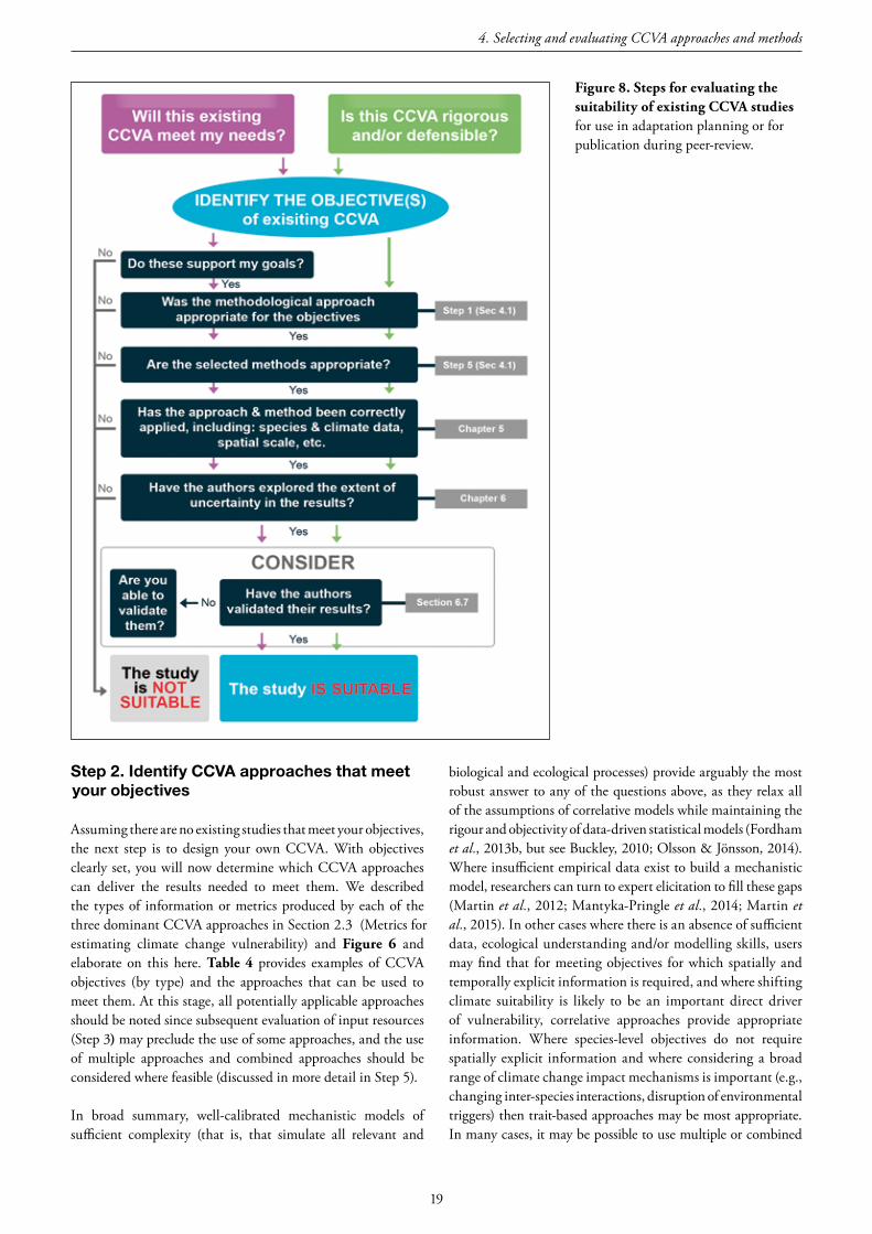
19

4. Selecting and evaluating CCVA approaches and methods

Figure 8. Steps for evaluating the suitability of existing CCVA studies for use in adaptation planning or for publication during peer-review.

Step2.IdentifyCCVAapproachesthatmeetyourobjectives

Assuming there are no existing studies that meet your objectives, the next step is to design your own CCVA. With objectives clearly set, you will now determine which CCVA approaches can deliver the results needed to meet them. We described the types of information or metrics produced by each of the three dominant CCVA approaches in Section 2.3 (Metrics for estimating climate change vulnerability) and Figure 6 and elaborate on this here. Table 4 provides examples of CCVA objectives (by type) and the approaches that can be used to meet them. At this stage, all potentially applicable approaches should be noted since subsequent evaluation of input resources (Step 3) may preclude the use of some approaches, and the use of multiple approaches and combined approaches should be considered where feasible (discussed in more detail in Step 5).

In broad summary, well-calibrated mechanistic models of sufficient complexity (that is, that simulate all relevant and

biological and ecological processes) provide arguably the most robust answer to any of the questions above, as they relax all of the assumptions of correlative models while maintaining the rigour and objectivity of data-driven statistical models (Fordham et al., 2013b, but see Buckley, 2010; Olsson & Jönsson, 2014). Where insufficient empirical data exist to build a mechanistic model, researchers can turn to expert elicitation to fill these gaps (Martin et al., 2012; Mantyka-Pringle et al., 2014; Martin et al., 2015). In other cases where there is an absence of sufficient data, ecological understanding and/or modelling skills, users may find that for meeting objectives for which spatially and temporally explicit information is required, and where shifting climate suitability is likely to be an important direct driver of vulnerability, correlative approaches provide appropriate information. Where species-level objectives do not require spatially explicit information and where considering a broad range of climate change impact mechanisms is important (e.g., changing inter-species interactions, disruption of environmental triggers) then trait-based approaches may be most appropriate. In many cases, it may be possible to use multiple or combined

20

IUCN SSC Guidelines for Assessing Species’ Vulnerability to Climate Change

approaches, thereby taking advantage of the strengths of component approaches (see Step 5 for further discussion).

Step3.IdentifytheCCVAapproachesforwhichyouhavesufficientresources

CCVA approaches and the methods used to apply them differ markedly in the resources they require, so the guidance we provide here is necessarily general. Very broadly, however, mechanistic approaches tend to be most resource intensive, with the simplest trait-based and tool-facilitated correlative approaches least so. In Table 5, we highlight the resources often required and/or desired to apply each of the three main CCVA approaches, discussing in turn: species distribution, trait and molecular data; climate data; ecological data; information on climate change impacts manifested indirectly through humans; expertise requirements; and final technological requirements.

Table 4.CCVA objective categories, examples of outputs required to meet them, and the approaches potentially able to deliver these. We note that combined CCVA approaches may also be applicable for meeting the examples specified. Thesuitabilityofeachcombinationtype(see Appendix Table D)formeetingobjectivesistypicallydependentonthatoftheirspecificcomponentapproaches.

CCVA Objective categories(fromTable1) Examples of CCVA outputs needed for addressing objectives

CCVAapproaches

Corr

elat

ive

Trai

t

Mec

hani

stic

Which?

Speciesvulnerabilityrankings Y Y Y

Subpopulationvulnerabilityrankingsorextinctionprobabilities Y Y

Speciesinvasionpotentialrankings Y Y Y

Howmuch?

Extinctionprobabilitiesofspeciesand/orpopulations Y

Estimatesofrangeshifts/changeinsuitableclimate-space(magnitude,distance,rate) Y Y

Dispersalpotential Y Y

Why?

Intrinsicclimatechangesusceptibility(i.e.,sensitivityand/oradaptivecapacity) Y Y

Identityofclimaticdriversofvulnerability Y Y

Identityofbiologicaldriversofvulnerability Y Y

Where?

Locationofareaswithgreatestconcentrationsofmostorleastvulnerablespecies Y Y Y

Locationofclimaticallysuitableorunsuitableareasforspeciesinfuture Y Y

Locationofpotentialcorridorsand/orrefugia Y Y

Subpopulationsoutsideprojectedsuitableclimates Y Y

Locationofareasmostimpactedbyspecificvulnerabilitydriversincludingdisruptionofinter-specificinteractionsandhumanresponsestoclimatechange

Y Y

When?

Timeframeofprojectedrisktospecies,sitesandlandscapes Y Y

Rateofshiftinclimatespace Y Y

Species/subpopulationpotentialturnoverrate Y Y

What’smissing?

Keygapsanduncertainties–climatic Y Y Y

Keygapsanduncertainties–biological Y Y

Keygapsanduncertainties–inourunderstandingofimpactsandtheirdrivingmechanisms Y Y Y

Keygapsanduncertainties–humanresponsestoclimatechangeasadriverofvulnerability# Y Y Y

SpeciesforwhichmoreinformationisneededtoenableCCVA# Thisisanactiveresearcharea–eachapproachmayinformatleastsomeaspectsofhowhumanresponsesmaydrivevulnerability.

We discuss each of these requirements briefly below in the context of this step, providing explanations using terminology and descriptions that are as simple and clear as possible; more detailed and rigorous guidance on selecting input data is provided later under Section 5.1 (Selecting and using input data). We highlight examples of free resources that may be of help to users (Table 6). Users may want to make use of Table  5 to record or highlight each resource type and information requirement evaluated, thereby noting where their resource strengths and gaps lie, and facilitating completion of this step. We include a row at the end of the table to record your feasibility conclusions. Finally, we note that, during evaluation of species data, users may recognize that their focal species is particularly poorly-known, small-range or a declined-range species (see Box 3), in which case users should see Section 4.2 (Approaches for three challenging CCVA situations: poorly-known, small-range and declined-range species).

21

Table 5.Summary of the data resources generally required by each CCVA approach.Wenotethatthesearebroadgeneralizationsandthatwithineachapproach,somemethodsrangefromresourcedemandingtomoreuser-friendly.Freelyavailabledatasourcesmeetsomeoftheneedsdescribed.

Resource type Input requirements Correlative Trait-based MechanisticSpeciesdistributiondata*

Pointlocalities;and/or Maybeused Maybeused Maybeused

Gridded/rasterdistributions;and/or Required Maybeused Generally required

Polygons/maps Maybeused(lessdesirable)

Generally required

Maybeused(lessdesirable)

Speciestraitdata* Demographictraits;and/orMorphologicaltraits;and/orBehaviouraltraits;and/orEcologicaltraits

Notused Required Required

Physiologicaltraits(e.g.,thermaltolerances,energyrequirements)

Notused Maybeused Required by some methods

Moleculardata Maybeused Maybeused Maybeused

Climatedata Distantpastorpaleoclimateprojections Maybeused Maybeused Maybeused

Recentpast/baselineclimateprojections Required Generally required

Required

Futureprojections Required Generally required

Required

Ecologicaldata Spatialprojectionsoflandcover(reflectingecosystem/habitat)

Maybeused Maybeused Maybeused

Spatialprojectionsofecologicalprocesses(e.g.,fire,hydrology,sealevelrise)

Maybeused Maybeused Maybeused

Datadescribingexacerbationofotherthreats(notcausedbyclimatechange)

Maybeused Maybeused Maybeused

IndirectImpacts Datadescribinghumanresponsestoclimatechange Notgenerallyused Maybeused Maybeused

Datadescribingclimatechangeinteractionswithotherthreats

Notgenerallyused Maybeused Maybeused

Expertise Toolsand/oruser-friendlyinterfacesavailable? Forsomemethods Forsomemethods

Forsomemethods

Speciesdistributionmodelling(assumingatoolisnotused) Required Notused Notused

GeographicInformationSystems(assumingatoolisnotused)

Required Generally required

Required

Speciesbiology Notused Required Required

Climateprojectionsandglobalscenarios Required Generally required

Required

Technologicalrequirements

Hardware(e.g.,computer) Required Generally required

Required

Software(additionaltoanoperatingsystemandspreadsheetapplication)

GISsoftwareoftenrequired

GISsoftwaremayberequired

GISsoftwareoftenrequired

Do your available resources meet the resource requirements?* Y/N/Maybe Y/N/Maybe Y/N/Maybe

* IMPORTANT:Ifyouknoworsuspectthatyourfocalspeciesmaybeorincludeapoorly-known, small-range or declined-range speciesthenpleaseseeBox 3andSection4.2(ApproachesforthreechallengingCCVAsituations).

4. Selecting and evaluating CCVA approaches and methods

21

Species distribution range data Species distribution range data are typically found in three forms. Point localities represent a collection of data points indicating locations where a species has been found to occur. They may have been collected as direct observations in the field (from atlases, surveys or citizen science programmes), or as spatial references for specimen collections held in museums or herbaria. These and other sources of distribution data may be accessible through portals or databases such as the Global Biodiversity Information

Facility (GBIF). Gridded data (or ‘raster data’) are based on presence and/or absence of a species within a mapped grid of variable size. Range polygons typically represent the maximum known extents of species’ distributions, whether globally or within a smaller geographical unit. If you know or suspect that your focal species may be or include a poorly-known, small-range or declined-range species then please see Box 3 and Section 4.2 (Approaches for three challenging CCVA situations: poorly-known, small-range and declined-range species).

22

IUCN SSC Guidelines for Assessing Species’ Vulnerability to Climate Change

Table 6 presents examples of sources of species distribution information. The IUCN Red List of Threatened Species is the largest repository of range polygons; other sources are also available, including field guides, action plans and journal papers. It is important to be aware that both range polygons and gridded data may include areas where a focal species does not occur (e.g., where a species occurs around a mountain but not on it, the map will typically include the mountain) and they therefore represent the limits of species’ distributions rather than the areas of occupancy. It may be desirable, depending on the intended use, to modify such data by removing areas of, for example, unsuitable habitat or elevation, that are known to exclude the species in question (e.g., Boitani et al., 2007; Beresford et al., 2011).

Species trait dataDemographic traits include information such as generation times, reproductive outputs, and longevity, while morphological traits relate to organisms’ sizes and shapes. Information on many of these per-species traits have been gathered from ex situ collections (e.g., zoos and botanical gardens); databases housing these data include Utheria (www.utheria.org) and the Zoological Information Management System (ZIMS; www.isis.org). It is important to recognize, however, that ex situ individuals may not always accurately reflect traits found in the wild (e.g., species may live much longer in captivity). Behavioural traits cover migratory, breeding, and dispersal habits, amongst others, and ecological traits provide information on species’ interactions with their

Table 6. Examples of data resources available for use in CCVA (adaptedfromPearson,2010).Thoselistedtendtofocusatglobalorcontinentalscales,butmanyregional-andnational-scaleresourcesarealsoavailable.

Examples of open access data sources for CCVA

Species data

Pointlocalitydistributiondata

GlobalBiodiversityInformationFacility(GBIF):pointdataavailablefor~1.5mspeciesglobally(dataneedtobe‘cleaned’beforeuse,e.g.,seeChapman,2005)

www.gbif.org

Griddeddistributiondata

FinnishBirdAtlas http://atlas3.lintuatlas.fi/background/copyrights

SouthAfricanBirdAtlasdata http://sabap2.adu.org.za/index.php

SouthAfricanFrogAtlasdata http://adu.org.za/frog_atlas.php

Distributionpolygons/maps

IUCNRedListDatabase(SpeciesInformationSystem):polygonsavailablefor~50,000speciesglobally,includingallmammals,birds,amphibians,cartilaginousfishandcorals

www.iucnredlist.org/technical-documents/spatial-data

NatureServe:polygonsavailableforWesternHemispheremammals,USfishesandListedandimperilledspecies

www.NatureServe.org

BirdLife:polygonsavailableforalltheworld’sbirdspecies(>10,000)

www.birdlife.org/datazone/info/spcdownload

Box3.TypesofspeciesthatposechallengestoCCVA

WeconsiderthreetypesoffocalspeciesthatcauseparticularchallengesforCCVA,anddiscussapproachesforcarryingouttheirCCVAsinSection4.2.

1.Poorly-knownspecies are those for which few data are available due to low sampling of their distributions and/or poor knowledge of their biology. This may be due to funding shortages, inaccessibility of these species’ habitats, low densities throughout their ranges or otherwise low detectability. Poor data availability is a serious challenge to CCVA using any of the conventional approaches, and is particularly acute in tropical regions (Feeley & Silman, 2011), which is also where the greatest biodiversity typically occurs (Gaston, 2000).

2.Small-rangespecies may or may not be locally common but occur only in a small area due to, for example, high climatic specialization (Ohlemüller et al., 2008), specific non-climatic requirements (Damschen et al., 2010), competition with other species, or geographic isolation (e.g., on islands). Small-range species can potentially be assessed using trait-based and mechanistic approaches, but assessments using correlative methods are inadvisable if the numbers of their occurrence records fall below the recommended thresholds (see Section 4.2 for further detail).

3.Declined-rangespecieshave extant ranges that are substantially smaller than their known ranges in recent history (nominally post-1750; longer or shorter timescales may be appropriate depending on the species); this decline may or may not have ceased. For the purposes of this discussion, we consider only those cases where declines are not caused by anthropogenic climate change. Declined-range species can generally be assessed using trait-based and mechanistic approaches, assuming that required data are available and that such approaches meet the assessors’ CCVA objectives (seeSection4.2;Tables4–5). They pose particular challenges, however, to correlative approaches because the extant range is unlikely to reflect the full breadth of the species’ environmental niche. Where ranges have declined such that the species occurs only in a small area, assessment challenges are compounded by those for small-range species.

23

Speciestraitdata IUCNRedListDatabase(SpeciesInformationSystem)

www.iucnredlist.org/

IUCN:climatechangesensitivityandadaptivecapacityrelatedtraitsforallbirds,amphibiansandcorals

Seesupplementaryinformationofwww.plosone.org/article/info%3Adoi%2F10.1371%2Fjournal.pone.0065427.Rawdataavailableonrequestfromredlist@iucn.org

Utheria:mammaltraits http://www.utheria.org/

TRY:planttraits http://www.try-db.org/

Traitnet:planttraits http://traitnet.ecoinformatics.org/

BirdLifeDataZone http://www.birdlife.org/datazone/home

Amphibiaweb http://amphibiaweb.org/

Biotraits:thermalresponsesofphysiologicalandecologicaltraits,especiallyconsumer-resourceinteractions(1,508spp)

http://biotraits.ucla.edu/

AfricanAlbertineRiftmammals,reptiles,freshwaterfishes,someplants

(Carret al.,2013).Scoresavailableinappendices:http://www.traffic.org/non-traffic/SSC-OP-048.pdf.Rawdataavailableonrequestfromredlist@iucn.org

Moleculardata Genbank:annotatedcollectionofallpubliclyavailableDNAsequences

http://www.ncbi.nlm.nih.gov/genbank/

Climate data

Distantpastorpaleoclimateprojections

NOAA http://www.ncdc.noaa.gov/data-access/paleoclimatology-data

ClimateResearchUnit(UniversityofEastAnglia) http://www.cru.uea.ac.uk/cru/data/paleo/

Recentpastorbaselineclimateprojections

Variousdatasetsbasedonmeteorologicalandsatellitedata.

SeeTable 8 fordetails.

Futureprojections IPCCDataDistributionCentre http://ipcc-data.org/

WORLDCLIM http://www.worldclim.org/

AFRICLIMforAfricanclimate https://www.york.ac.uk/environment/research/kite/resources/

Ecological data

Landcoverandecologicalprocesses

GlobalLandcoverFacility:landcoverandotherproducts,floods

http://glcf.umd.edu/data/

NASA(MODIS):Landcover,cloudcover,firefrequency

https://lpdaac.usgs.gov/products/modis_products_table/modis_overview

USGS:Elevationandrelatedvariablesfortheglobe(1km2)

http://edc.usgs.gov/products/elevation/%20gtopo30/hydro/index.html

SRTM:Digitalelevationmodel(90m2) http://www.cgiar-csi.org/data/srtm-90m-digital-elevation-database-v4-1

Soiltype:UNEP http://www.grid.unep.ch/data/data.php?%20category=lithosphere

Watersheds(orhydrobasins): Lehner and Grill (2013)

http://hydrosheds.org/

NOAA:Variousoceanographicproducts http://www.nodc.noaa.gov/access/

Humanresponsestoclimatechange

HumanvulnerabilitytoclimatechangeinSouthernAfricaby2050(Midgleyet al., 2011)

http://www.parcc-web.org/parcc-project/documents/2012/12/climate-risk-and-vulnerability-mapping-for-southern-africa-status-quo-2008-and-future-2050.pdf

Technical resources

Geospatialanalyses QuantumGIS http://www.qgis.org/en/site/

GRASSGIS http://grass.osgeo.org/download/

WorldMap http://worldmap.harvard.edu/

R https://www.r-project.org/

Python https://www.python.org/

SoftwareforAssistedHabitatModelling(SAHM) https://www.fort.usgs.gov/products/sb/5090

Correlativemodellingsoftware

Maxent https://www.cs.princeton.edu/~schapire/maxent/

openModeller http://openmodeller.sourceforge.net/

Table 6 cont’d. Examples of data resources available for use in CCVA (adaptedfromPearson,2010).Thoselistedtendtofocusatglobalorcontinentalscales,butmanyregional-andnational-scaleresourcesarealsoavailable.

4. Selecting and evaluating CCVA approaches and methods

Examples of open access data sources for CCVA

24

IUCN SSC Guidelines for Assessing Species’ Vulnerability to Climate Change

environments and include their habitat requirements, inter-species interactions and reliance on environmental triggers.

Traits of relevance for CCVA frequently differ between taxonomic groups; for corals, for example, the types of species’ algal symbioses are of importance for climate change vulnerability, while for aquatic plants, salt tolerance may be key. Sources of trait information include online databases (see Table 6), formal and grey literature, field guides, the IUCN’s Species Information Service (SIS), and experts’ knowledge. In cases where specific data are not available, it may be possible to infer traits from closely related taxa or from other characteristics (e.g., inference of dispersal ability and feeding guild from morphological traits) (see Hespenheide (1973) for a review), providing a potentially very valuable source of information for poorly known species.

Data on physiological traits such as thermal tolerances and energy requirements can be extremely valuable for climate change vulnerability assessments since they allow more confident predictions of species’ fundamental niches and hence more robust range predictions (Kearney & Porter, 2009). These data are, however, amongst the most challenging to source. Laboratory experiments and records for species held ex situ provide the main sources of such information, but studies of in situ physiological responses may also be found in formal and grey literature. As with demographic trait data, physiological trait data tend to be restricted to a few well-studied species, and caution should be exercised in extrapolating data from ex situ records. Physiological traits are valuable for trait-based approaches, essential for mechanistic approaches, and can be incorporated in correlative-mechanistic approaches.

Molecular information Molecular data, including on neutral genetic markers, can help to determine population processes including dispersal and population size fluctuations. Recent advances in sequencing technology now allow these processes to be accurately traced based on thousands of genetic markers – an increase of three orders of magnitude over recent years. Moreover, the markers can be linked to genes under selection and involved in adaptation. This can be used to investigate both past adaptation to different environments (using a correlative approach) and potential for future adaptation (informing mechanistic models and viability analyses).

Molecular data may be used to estimate species’ potential for adaptation but they do not easily indicate the extent to which adaptive shifts will impact upon the traits that influence species’ distribution and abundance. This requires quantitative genetic assessment of variation within and among populations, which can be more difficult to undertake than molecular studies, particularly in species with long generation times. However, there is potential to combine genomic data with phenotypic studies to evaluate the extent to which traits might be shifted by rapid evolution. Genetic

data are generally available for small numbers of species only (e.g., see Table 6).

Generally applications of correlative models assume that populations of species respond to climate change in the same manner across their range. However, local adaptation can enhance fitness of populations to their immediate environment at the expense of reducing their niche breadth compared to the species as a whole (Shaw & Etterson, 2012). When this occurs, applying a correlative model to a species as a whole could overestimate the species’ ability to withstand anticipated climate change (O’Neill et al., 2008; Pearman et al., 2010; Valladares et al., 2014; Hällfors et al., 2016). In this context, molecular data can be used as a proxy for the spatial scale of local adaptation within a species by, for example, allowing assessors to divide species into mutually exclusive subgroups (lineages) and estimating vulnerability for each group separately (e.g., Pearman et al., 2010; Hällfors et al., 2016).

Climate dataWe briefly discuss three categories of climate data here, but provide more detailed explanations, including on their use, in Section 5.1.3 (Climate datasets). Distant past or paleoclimate projections can extend climate records from hundreds to millions of years, and are derived using proxy methods such as dissolved isotopes in sediments and ice, or from plant growth rates inferred from fossilized tree rings (Folland et al., 2001). They can be used to train and test correlative models’ predicted species distributions by developing climatic correlations based on longer, historical time scales (Lawing & Polly, 2011). In order to achieve this, historical species distribution data, typically inferred from fossil evidence, are also required. Both data types are subject to uncertainties associated with reliability of the original samples and the interpolation techniques used, and these should be borne in mind when using them to make inferences about current and future species distributions. Various paleoclimatological data sets are available (see Table 6). They may potentially be used by all CCVA approaches, but have most often been associated with correlative approaches (e.g., Huntley et al., 2006).

Recent past or baseline climate data aim to represent the conditions at the onset of the impacts of anthropogenic climate change (i.e., typically from the half-century prior to 2000). A fundamental distinction is that baseline climate data are derived from actual meteorological station observations whereas future climate projections are derived from models (GCMs). Baseline climate data are used to infer the climatic conditions at which species’ distributions are assumed to have been at equilibrium, and hence are important for identifying the variables by which each species is theoretically constrained. As such, they are used to train correlative models as a basis for future projections, and they form an essential reference point for all measures of projected future change. All CCVA approaches require the use of baseline climate observations, with the occasional exception of some trait-

25

based approaches in which distribution range data are lacking or where assessments of biological susceptibility alone are required. We discuss baseline climate datasets in more detail in Section 5.1.3 (Climate datasets), and provide examples of available datasets in Table 8.

Future projections of climate are produced by GCMs, which are computationally intensive mathematical models that simulate atmosphere and ocean processes, including sea ice and land-surface components, for weather forecasting and projecting climate change. Many groups and laboratories around the world run GCMs to produce projections of future climates, and each model is run multiple times to accommodate uncertainties in natural components such as cryospheric (snow and ice) feedback (i.e., the amplification or moderation of physical changes by snow or ice environments), as well as uncertainties in anthropogenic variables including future greenhouse gas emissions. Uncertainty from different emissions scenarios is modelled according to a series of plausible scenarios of expected atmospheric CO2 concentrations, the most recent of which are those defined by the Representative Concentration Pathways (RCP’s) associated with the Fifth (latest) IPCC report (Moss et al., 2010; IPCC, 2013b).

While the various models and their runs all produce projections, none perfectly reproduces the climate systems being modelled and numerous uncertainties remain. As a result, use of a number of models and runs is recommended. Maintaining and using a measure of the disagreement between models is extremely important for understanding the uncertainties in predictions and accommodating and communicating them in subsequent use (see Section 5.1.3 (Climate datasets) for further discussion, including on selection of model, emissions scenarios and bioclimatic variables).

The IPCC’s Data Distribution Centre (http://ipcc-data.org/) is a portal for access to a broad range of future climate datasets. Reference to the associated ‘Guidance on use of data’ section (including technical guidelines, fact sheets, supporting material, scenario processes, definitions, etc.) is strongly recommended. As with baseline climate data, future climate projections are needed for all CCVA approaches, except where trait-based methods are used either in the absence of distribution range data or for simplistic, preliminary CCVAs. For correlative and mechanistic models, future climate projections are used to project future climatic suitability of landscapes, and for trait-based approaches, to project climate change exposure across species’ current ranges.

Ecological dataSpatially-explicit landcover (representing ecosystems and/or habitats), elevation and soil type datasets have been used in various ways in CCVAs, and are relevant for all three CCVA approaches. We discussed previously how habitat and elevational associations may be used to refine species’ distribution range maps (i.e., by removing areas of unsuitable

habitat and elevation where the species is known not to be able to occur (Boitani et al., 2007; Beresford et al., 2011; Foden et al., 2013)). They may also be used in combination with future climate projections to create more refined estimates of future suitability of each landscape component/grid cell for focal species. Spatial projections of ecosystem processes such as fire, sea level rise and hydrology may also be used for this purpose. For example, Aiello-Lammens et al. (2011) used landcover, elevation, projected sea level rise and a range of site-specific information including erosion rate, storm frequency and tidal trends to predict sea level rise impacts on Snowy Plovers in Florida. These land- and seascape-scale physical and ecological data have been used in correlative, mechanistic, trait-based and combined approaches. Uncertainties in such data should be carefully noted. Further discussion on this subject is included in Section 5.1.6 (Accounting for habitat availability).

Indirect climate change impacts Biodiversity threats caused by indirect impacts of climate change have been poorly recognized in CCVA to date, despite their potential to overwhelm direct climate change impacts on species (Turner et al., 2010; Maxwell et al., 2015). We consider such indirect impacts to include those due both to human responses to climate change (e.g., expansion of biofuel plantations; construction of dams and sea walls, expansion into newly suitable agricultural or fishing zones) and to the natural systems that focal species inhabit (e.g., increased exposure and susceptibility to pathogens and invasive species; declining resource availability). These impacts can interact with non-climatic threats, potentially greatly magnifying their impacts. Mechanistic and trait-based approaches typically accommodate consideration of changes in inter-species interactions and all approaches implicitly incorporate aspects of changing habitat suitability. Few, however, consider human responses to climate change, or the interacting effects of climate change on non-climatic threats. This important yet neglected aspect of CCVA is discussed in more detail in Section 5.2.1 (Direct versus indirect impacts of climate change).

ExpertiseWe assume that practitioners have the expertise to make use of conventional computer software (e.g., Microsoft Excel), and here distinguish two main additional types of expertise, namely technical and biological. We note that CCVAs are often carried out by teams, making assembling suitable combinations of expertise easier.

The technical expertise needed to apply trait-based approaches is often relatively low, involving gathering information in, for example, a spreadsheet, and using simple calculations to combine these into overall rankings or scores. The level of expertise needed to assess species’ exposure to climate change varies from very low where, for example, simple overlays of pre-processed climate surfaces (e.g., www.climatewizard.org for the USA) are used, to more complex with the requirement of proficiency in Geographic Information Systems (GIS) for

4. Selecting and evaluating CCVA approaches and methods

26

IUCN SSC Guidelines for Assessing Species’ Vulnerability to Climate Change

others. NatureServe’s Climate Change Vulnerability Index (CCVI, Young et al., 2011) is a well-documented, user-friendly tool that provides a low-technical-expertise CCVA option.

The numerous methods available to carry out correlative and mechanistic CCVA approaches preclude generalization about the levels of technical expertise they require. Some statistically complex approaches provide user-friendly interfaces (e.g., MaxEnt; BIOMOD) and hence require little technical expertise to run, while others require a knowledge of programming languages such as R and/or extensive GIS skills. We strongly urge users to familiarize themselves with the technical aspects of even user-friendly methods since this is essential if their settings are to be correctly parameterized, sensitivity tested and their results responsibly interpreted. It is also advisable for assessors to understand the methods used to prepare climate projection data for use, since their assumptions, uncertainties and downscaling approaches are all important CCVA parameters. More information on these is available in Section 5.1.3 (Selecting and using climate datasets).

Biological expertise is highly desirable and in many cases essential for CCVA. In their most simple form, correlative approaches can be based purely upon distribution data, but without biological expertise errors may not be identified and results can easily be misinterpreted. A thorough understanding of a species’ dispersal mechanisms, dispersal and colonization potential, and its biological requirements are all important aspects of translating correlative model outputs into vulnerability assessments. Trait-based assessments require, by definition, knowledge of a species’ biology and ecology, and mechanistic (including combined correlative-mechanistic) approaches generally have the most intensive requirements for biological expertise, since users must select not only which variables to include but also how these should be parameterized and how they interact with each other. Biological expertise is also particularly important for evaluating where and how information gaps may be filled using, for example, inferred or proxy traits.

Technical requirementsA spreadsheet application may be all that is required for simple assessments (e.g., trait-based; NatureServe’s CCVI (Young et al., 2012)), but where datasets become large (e.g., >100,000 records), storage capacity and functionality of such software may become limiting. Databases such as Microsoft Access and Microsoft SQL Server are more stable, much faster, allow bulk processing of large repeated calculations and have easily customizable functions. The benefits of more sophisticated software must be traded, of course, against purchase costs and the time and effort needed to learn to operate it. The statistical language and programming environment R (also called GNU S) is gaining increasing popularity and use as it is an open-source software package which allows storage and analysis of large datasets.

A number of software packages are available which are designed specifically for the analysis and prediction of species

distributions (i.e., correlative approaches); these include MaxEnt, ModEco and many R packages, among numerous others. Each of these packages requires some training for responsible application and for interpreting their outputs, and each has a range of advantages and disadvantages relative to the others. Examples of different method and models are provided in Appendix Tables A–D.

Finally, although many software packages include a spatial component, assessors will often find it useful to work with a standalone GIS software package, particularly when constructing maps to display assessment results. The most commonly used GIS software package is ArcGIS, but open access GIS packages such as QGIS, DIVA-GIS (designed with species distribution modelling processes in mind), PostgreSQL and PostGIS, among others, will often be more than sufficient. A range of additional software packages designed to link to GIS software and to conduct specific CCVA-relevant analyses are available. One such package is RAMAS GIS, a programme designed to combine geographic and demographic species data in order to conduct spatially-explicit population viability analyses. Again, we reiterate that the software packages listed here are only a handful of examples of a much wider available range, and we encourage assessors to explore other options that may be available to suit their needs.

The specifications of computing hardware required are mostly governed by the total size of the data to be processed, and the complexity of the operations to be undertaken. Data size is, in turn, determined by numerous factors, including the spatial resolution of geospatial coverages (e.g., climatic data, land cover), the geographic scope of the assessment, and the number of species under assessment, among others. In general, the greater the storage capacity available, and the faster the processing power of the computer, the better, and in some cases it may be necessary to use external data storage devices and advanced ‘supercomputer’ hardware. At worst, undertaking assessments with insufficient data storage or processing capacity will mean that operations fail to execute, although often it can simply result in processes taking large amounts of time. Assessors with limited hardware capacity may need to compromize between the time they are willing to allow for processes to compute and the scope or complexity of their assessment.

Step4.DoSteps2and3identifyanyofthesameapproaches?

The objective of this step is to identify the one or more CCVA approaches that both meet objectives and for which sufficient resources are available. Under ideal circumstances, users may find overlap in multiple approaches, and under somewhat less ideal circumstances, users might find overlap in only one approach between those selected according to objectives and those by resources. Nonetheless, both of the above circumstances allow practitioners to proceed to the next steps.

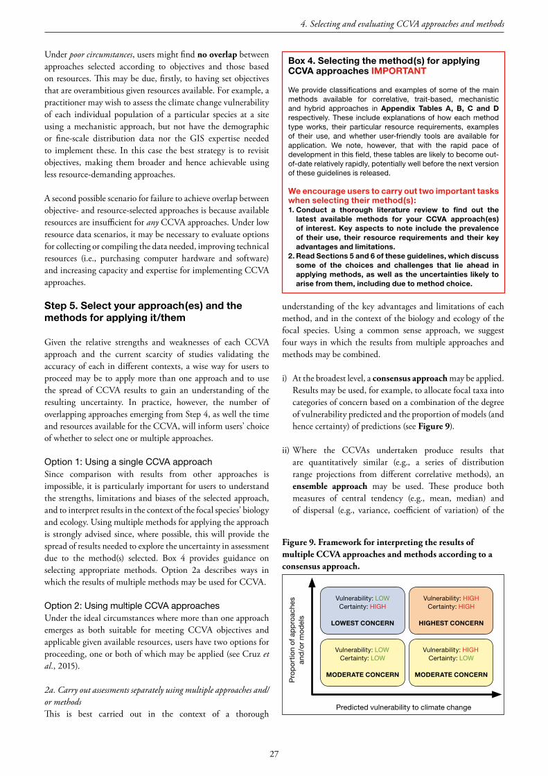
27

Under poor circumstances, users might find no overlap between approaches selected according to objectives and those based on resources. This may be due, firstly, to having set objectives that are overambitious given resources available. For example, a practitioner may wish to assess the climate change vulnerability of each individual population of a particular species at a site using a mechanistic approach, but not have the demographic or fine-scale distribution data nor the GIS expertise needed to implement these. In this case the best strategy is to revisit objectives, making them broader and hence achievable using less resource-demanding approaches.

A second possible scenario for failure to achieve overlap between objective- and resource-selected approaches is because available resources are insufficient for any CCVA approaches. Under low resource data scenarios, it may be necessary to evaluate options for collecting or compiling the data needed, improving technical resources (i.e., purchasing computer hardware and software) and increasing capacity and expertise for implementing CCVA approaches.

Step5.Selectyourapproach(es)andthemethodsforapplyingit/them

Given the relative strengths and weaknesses of each CCVA approach and the current scarcity of studies validating the accuracy of each in different contexts, a wise way for users to proceed may be to apply more than one approach and to use the spread of CCVA results to gain an understanding of the resulting uncertainty. In practice, however, the number of overlapping approaches emerging from Step 4, as well the time and resources available for the CCVA, will inform users’ choice of whether to select one or multiple approaches.

Option 1: Using a single CCVA approachSince comparison with results from other approaches is impossible, it is particularly important for users to understand the strengths, limitations and biases of the selected approach, and to interpret results in the context of the focal species’ biology and ecology. Using multiple methods for applying the approach is strongly advised since, where possible, this will provide the spread of results needed to explore the uncertainty in assessment due to the method(s) selected. Box 4 provides guidance on selecting appropriate methods. Option 2a describes ways in which the results of multiple methods may be used for CCVA.

Option 2: Using multiple CCVA approachesUnder the ideal circumstances where more than one approach emerges as both suitable for meeting CCVA objectives and applicable given available resources, users have two options for proceeding, one or both of which may be applied (see Cruz et al., 2015).

2a. Carry out assessments separately using multiple approaches and/or methodsThis is best carried out in the context of a thorough

understanding of the key advantages and limitations of each method, and in the context of the biology and ecology of the focal species. Using a common sense approach, we suggest four ways in which the results from multiple approaches and methods may be combined.

i) At the broadest level, a consensus approach may be applied. Results may be used, for example, to allocate focal taxa into categories of concern based on a combination of the degree of vulnerability predicted and the proportion of models (and hence certainty) of predictions (see Figure 9).

ii) Where the CCVAs undertaken produce results that are quantitatively similar (e.g., a series of distribution range projections from different correlative methods), an ensemble approach may be used. These produce both measures of central tendency (e.g., mean, median) and of dispersal (e.g., variance, coefficient of variation) of the

Box4.Selectingthemethod(s)forapplyingCCVAapproachesIMPORTANT

We provide classifications and examples of some of the main methods available for correlative, trait-based, mechanistic and hybrid approaches in Appendix Tables A, B, C and D respectively. These include explanations of how each method type works, their particular resource requirements, examples of their use, and whether user-friendly tools are available for application. We note, however, that with the rapid pace of development in this field, these tables are likely to become out-of-date relatively rapidly, potentially well before the next version of these guidelines is released. Weencourageuserstocarryouttwoimportanttaskswhenselectingtheirmethod(s):1. Conduct a thorough literature review to find out the

latest available methods for your CCVA approach(es)of interest.Keyaspects tonote include theprevalenceof their use, their resource requirements and their keyadvantagesandlimitations.

2.ReadSections5and6oftheseguidelines,whichdiscusssome of the choices and challenges that lie ahead inapplyingmethods,aswellastheuncertainties likelytoarisefromthem,includingduetomethodchoice.

Figure 9. Framework for interpreting the results of multiple CCVA approaches and methods according to a consensus approach.

Predicted vulnerability to climate change

Pro

po

rtio

n of

ap

pro

ache

san

d/o

r m

od

els

Vulnerability: LOWCertainty: HIGH

LOWESTCONCERN

Vulnerability: HIGHCertainty: HIGH

HIGHESTCONCERN

Vulnerability: LOWCertainty: LOW

MODERATECONCERN

Vulnerability: HIGHCertainty: LOW

MODERATECONCERN

4. Selecting and evaluating CCVA approaches and methods

28

IUCN SSC Guidelines for Assessing Species’ Vulnerability to Climate Change

CCVA results. We note that the results of methods from within the same approach are likely to be correlated, and that between-approach comparisons are likely to introduce a broader spread of results, suggesting that varied weighting of results might be appropriate.

iii) Using upper and lower projection bounds or extremes to propose best and worst case scenarios (with a plausible range of possibilities between these), may be useful when CCVA results are qualitatively different, and this may be applied in conjunction with a consensus approach (suggestion (i)).

iv) In cases where CCVA results differ markedly and evidence supporting either is lacking, users could choose to follow the precautionary principle and take the highest vulnerability assessment as the basis for determining the level of concern for the focal taxa.

Irrespective of which of the above approach(es) is selected, it is important to investigate the reasons for the inevitable spread in the results. This may expose any errors in the assessment and greatly increases the strength of conclusions drawn from the results.

2b. Combine approachesHybrid CCVA approaches which combine elements from two or more approaches have begun to emerge, and these potentially draw on the strengths of their component methods. We summarize six emerging types of these, briefly describing how they work, tools available, resources required and published examples (Appendix Table D); they include combinations of correlative-trait-based, correlative-mechanistic and correlative-mechanistic-trait-based approaches. Willis et al. (2015) identify the multiple ways in which correlative and trait-based approaches may be integrated, including for use for spatial conservation planning; they suggest that correlative approaches may benefit from trait-based measures of sensitivity (e.g., known climatic tolerances) and adaptive capacity (including dispersal capacity) (e.g., Warren et al., 2013), while trait-based approaches may be strengthened by using correlative-derived distribution range projections to quantify climatic tolerances and climate change exposure (e.g., Thomas et al., 2011; Young et al., 2011a; Smith et al., 2016).

The use of traits to inform projections of species’ dispersal and colonization capacities in particular has begun to receive attention. Estrada et al. (2016) outline framework highlighting how four key range-shift processes are affected by seven trait types, namely (with traits in brackets): (i) emigration (site fidelity); (ii) movement (movement ability); (iii) establishment (avoidance of small population effects, persistence under unfavourable conditions); and (iv) proliferation (reproductive strategy; ecological generalization and competitive ability (these three traits apply to processes (iii) and (iv)). Garcia et al. (2014) use traits to identify regions where correlative-based range projections may under- or overestimate assessments of climate change

vulnerability for species, while Visconti et al. (2015) used species-specific dispersal distances and generation length estimates to account for species’ ability to keep track of their projected shifting bioclimatic ranges. We discuss some of the challenges and uncertainties in the use of such trait data in Section 6.5 (Uncertainty from biological trait and demographic data).

4.2 ApproachesforthreechallengingCCVAsituations:poorly-known,

small-anddeclined-rangespecies

Availability of suitable data is a prerequisite for the conventional CCVA approaches outlined so far in these guidelines. Three types of species present particular challenges for their application: poorly known, small-range and declined-range species (see Box 3). “Poorly-known species” are problematic when scarce data on occurrences, traits or physiology preclude application of correlative, trait-based or mechanistic approaches, respectively. Challenges also arise in the particular case where occurrence data exist, but the characteristics of the focal species render the data inadequate for application of correlative CCVA approaches. This is the case for “small-range species” that have naturally small ranges due to, for example, high specialization, as well as for “declined-range species”, whose ranges have become smaller due to anthropogenic (non-climatic) threats.

Large numbers of poorly-known species lack biological data for trait-based or mechanistic approaches, particularly those with smaller body sizes and more restricted ranges (González-Suárez et al., 2012). Many poorly-known species, as well as small- and declined-range species, also lack sufficient occurrence data for correlative modelling. Because correlative approaches must statistically characterize the relationships between a species’ current range and the bioclimatic variables historically occurring there, they require a minimum number of species

The Keel-billed Toucan (Ramphastos sulfuratus) in Costa Rica has moved its habitat from the lowlands and foothills up to at least 1,540 m following increased cloud-base levels due to climate change. © Andy Morffew

29

occurrence records to ‘learn’ from in order to produce reliable results. The IUCN Standards and Petitions Subcommittee (IUCN, 2014) recommends that, as a general rule, at least five species occurrence records or ‘presence’ grid cells are required for each bioclimatic variable used (see Section 5.1.4 (Selecting and using species distribution data)); other authors suggest a minimum of 10, 50 or 100 records in total, depending on the model type and complexity, and the species under study (Stockwell & Peterson, 2002; Wisz et al., 2008). Species with occurrence data that do not meet these requirements are thus usually not modelled.

Many broad-scale assessments to date have been based on multi-species correlative approaches (e.g., Thomas et al., 2004; Araújo et al., 2006; Thuiller et al., 2011; Warren et al., 2013). While in some cases the species coverage is excellent (e.g., 90% of native European breeding birds; Huntley et al., 2008), it is more typical for a high proportion of species to be omitted due to insufficient records, especially in the most biodiverse regions. For example, in an assessment for African vertebrates (Garcia et al., 2012), only 33% of recorded species were modelled. Platts et al. (2014) found that species omitted from correlative CCVA in sub-Saharan Africa represented 92% of the region’s threatened amphibians, and that records for the omitted species spanned different climatic conditions and different rates of climate warming, compared to modelled species. These examples highlight that conventional CCVA methods are potentially restricted to a biased sample of species, rendering conclusions about the impacts of climate change on biodiversity incomplete (Schwartz et al., 2006; Platts et al., 2014).

The spatial resolution of the climate data used in correlative models is of strong importance, since distribution data will need to be modelled at the same scale. For climate data at one-degree resolution, for example, a small-ranged species may occur in only a handful of ‘presence’ grid cells (111 x 111 km at the equator), even though hundreds of locality records may exist within these. This challenge may be alleviated for some species by increasing spatial resolution (and hence decreasing grid size) of the climate data using process-based, statistical or empirical downscaling. However, for species with very few locality records or particularly small ranges, and those for which lower spatial resolutions are necessary (e.g., fine-scale occurrence data not available, or data processing capacity is limited), this challenge remains.

We outline below five broad approaches for addressing the challenges of carrying out CCVA on poorly-known, small-range or declined-range species. The first (i) is to gather data to allow conventional approaches to be used. The second (ii) considers a situation where time-series of population and climate data are available. The other three describe alternative CCVA approaches that allow CCVA to be carried out despite poor information. They include (iii) modifications of familiar correlative techniques, (iv) selecting alternative taxonomic foci for the models, and (v) implementing

assessments that consider exposure of geographical areas rather than particular species’ distributions. The five alternative approaches are summarized in Table 7 (over).

i)Filldatagaps

Poorly-known speciesThe first option is to gather the missing data that are required for application of conventional correlative, trait-based or mechanistic models. For missing trait data, expert inference can often be made from related species, for example from higher taxonomic ranks (Foden et al., 2013). Data gaps can be filled through either eliciting expert opinion (Murray et al., 2009a; Flockhart et al., 2015) or using data imputation techniques applied to datasets covering related species (Buckley & Kingsolver, 2012; Swenson, 2014; Taugourdeau et al., 2014; Schrodt et al., 2015). Where the option of filling data gaps is pursued, it is advisable to assess the sensitivity of the results to different opinions/techniques, by comparing inference derived under sets of ‘optimistic’ versus ‘pessimistic’ assumptions. For example, an unknown trait can be scored as either detrimental or beneficial to a species’ chances of survival under climate change; the extent to which these opposing assumptions affect the overall outcome of the CCVA provides a measure of uncertainty associated with the gap filling undertaken (Martin et al., 2012; Penone et al., 2014; Meng et al., 2016).

In cases where, based on expert opinion or literary accounts, it is suspected that the distribution records available for CCVA under-represent a species’ true range, the estimation of the range could be systematically improved through iterative application of modified correlative techniques (see c), or by reference to literature, together with targeted fieldwork (Williams et al., 2009; Platts et al., 2010).

Declined-range speciesIn cases where threats unrelated to climate change are known to have reduced the species’ range significantly, inclusion of the historical range can render conventional modelling applicable while allowing for a wider range of suitable environmental conditions to be captured in the model. However, here it becomes essential to control for the likely reasons for range decline in the model or in post-modelling analyses.

ii)Temporalanalysisofpopulationvariability

Small-range and declined-range speciesFor species with insufficient occurrence records for correlative modelling, or for which the recorded or modelled spatial distribution does not provide a good representation of the climatic niche (e.g., edaphic specialists), temporal analysis of population variability could provide useful information about the vulnerability of populations, and species as a whole, to projected changes in climate (Damschen et al., 2010). This approach requires robust time-series of inter-annual population variability, both in terms of sampling rigor and in the length

4. Selecting and evaluating CCVA approaches and methods

30

IUCN SSC Guidelines for Assessing Species’ Vulnerability to Climate Change

of the record, and thus will apply to a relatively small subset of species. Assessors should be aware that, especially for species with naturally high inter-annual population variability, short time-series and/or few time-points could result in spurious detection of a climate change effect (McCain et al., 2016).

Given sufficient data, a typical approach is to perform a linear regression, wherein the dependent variable is the change in population size relative to the previous year (often log-transformed), and the independent variables are measures of climate experienced by the population in the preceding year(s). Annualized climate data are available for most parts of the world, in some cases dating back to the beginning of the 20th century (e.g., CRU goes back to 1901; satellite products back to

the 1980s (CHIRPS, TAMSAT) or early 2000s (MODIS); see Table 8 and Section 5.1.3.3 (Historical (baseline) datasets)). To control for density-feedback, the population size in the previous year is sometimes included as a covariate in the model. If population data are available for more than one site within the species’ range, these can be included in the same model, with differences across sites controlled for by including site as a random factor (mixed modelling; e.g., Bennie et al., 2013).

Temporal analysis of population variability has been used to assess climate change impacts on bird communities (Pearce-Higgins et al., 2015) and Lepidoptera in the United Kingdom (Bennie et al., 2013; Martay et al., 2016). Most examples to

Table 7. Approaches for three challenging CCVA situations.

Poorly-known species Small-range species Declined-range species (not climate related)

Conventional approaches

Correlative models

Statisticallyproblematicwhereoccurrencerecordsareinsufficient

Statisticallyproblematicduetoinsufficientoccurrencerecords

Problematicsinceextantrangecannotbeusedtoinferenvironmentalniche

Mechanistic models

Problematicwheremechanisticinformationisinsufficient

Applicableifmechanisticdataavailable Applicableifmechanisticdataavailable

Trait-based models

Problematicwheretraitinformationisinsufficient

Applicableiftraitdataavailable Applicableiftraitdataavailable

Alternative approaches

i) Fill data gaps Highpriority;dataadditionorinferencemayrenderallconventionalapproachesapplicable

BeneficialforcorrelativeapproachesifnewdataextendknowndistributionrangeNewtraitdatamayrenderconventionaltrait-basedandmechanisticapproachesapplicable

Additionaldataonextinctlocalitiesorrangeareadvisabletocomplementextantoccurrencerecordsforcorrelativemodelling(thusincreasingenvironmentalnichecoverage).Additionaltraitdatalikelytorenderconventionaltrait-basedandmechanisticapproachesapplicable

ii) Temporal analysis of population variability

Problematicwheretime-seriesinformationisinsufficient

Potentiallyapplicable,ifrobusttime-seriesofinter-annualpopulationvariabilityareavailable.Underlyingdemographicprocessesshouldbecarefullyconsidered

Potentiallyapplicable,ifrobusttime-seriesofinter-annualpopulationvariabilityareavailable.Underlyingdemographicprocessesshouldbecarefullyconsidered

iii) Modified correlative techniques

Potentiallyapplicable;advantageouswhenspecies-levelresultsareessential,althoughresultswillbelessreliable

Potentiallyapplicable,andadvantageouswhenspecies-levelresultsareessential

Potentiallyapplicable,butimportanttoensurethatpredictorsassociatedwithdeclineareincludedinmodelorusedtofiltermodelprojections

iv) Alternative taxonomic focus

Assessingassemblagesofassociatedspeciesisapplicablewhenspecies-levelresultsarenotessential.Thiscanbeappliedusingconventionalcorrelativeandtrait-basedapproaches

Applycorrelativemodelstointeractingspecies,particularlywherecloselycoupledtothefocalspecies(e.g.,specialistresourcespeciesorclosecompetitors).Assessingassemblagesofassociatedspeciesisapplicablewhenspecies-levelresultsarenotessential;thiscanbeappliedusingconventionalcorrelativeortrait-basedapproaches

Asfor‘small-rangespecies’.Assessingassemblagesisparticularlyrelevantwheretheyshareacommonreasonfordecline.Ensurethatpredictorsassociatedwithdeclineareincludedinmodelorusedtofiltermodelprojections

v) Exposure assessment of geographic area

Potentiallyapplicableifregionofoccurrenceisknownandwhenspecies-levelresultsnotessential

Applicablewhenspecies-levelresultsnotessential;potentialtomakeresultsmorespecies-specificbyusingtraitstointerpretlikelythreatsandopportunitiesarisingduetoregion’sexposuretoclimatechanges

Applicablewhenspecies-levelresultsnotessential;potentialtomakeresultsmorespecies-specificbyusingtraitstointerpretlikelythreatsandopportunitiesarisingduetoregion’sexposuretoclimatechangesandbyconsideringimpactsondriversofspeciesdecline

31

date have not specifically targeted small-range or declined-range species, but the approach is applicable regardless of range size. A representative sample across the known species’ range will, however, increase confidence in the climate drivers identified (Cayuela et al., 2016).

If a climate change signal is reliably detected from historical time-series, vulnerability to projected future changes in climate may be inferred from long-term trends in the aspects of climate identified as potentially important in driving population change (e.g., increased seasonality or inter-annual variability in rainfall, or mean annual warming).

iii)Modifiedcorrelativetechniques

Small-range speciesSpecies with low numbers of occurrence records have in some cases been modelled using the simplest of “envelope” correlative techniques (Busby, 1991a), defined by the range of values occupied by a species across a set of relevant predictors. One example is the application of multidimensional niche envelopes to African amphibians (Platts et al., 2014). In order to include even those amphibians with a single, coarse-resolution, gridded occurrence record, the envelopes were defined by the interquartile range of finer-resolution climatic conditions within those cells. Drawbacks of this highly simplified approach include that model performance (i.e., the model’s ability to accurately predict across space or time) is difficult to assess, that all predictors are given equal weight in limiting the species’ distribution, and that environmental conditions beyond the observed niche are generally considered wholly unsuitable, which is problematic if the species has been under-sampled. Most other correlative methods permit non-zero predictions beyond the observed niche, but are still subject to high model uncertainty, particularly when applied to small sample sizes (Thuiller et al., 2004; Pearson et al., 2006).

In another application (Hof et al., 2011), also for amphibians but at a global scale, the assessment of all species was possible with the use of simple distance-based correlative models (Euclidean and Mahalanobis distance, which measure the similarity of species’ occurrences to the mean or centre of the available climatic space). More complex correlative modelling techniques can also be adapted to cater for small numbers of occurrences; adjustment of the “regularization multiplier” in MaxEnt, which controls the degree of model overfitting, is an example (Hof et al., 2011). Alternatively, models can be restricted to small numbers (e.g., two) of relevant environmental predictors, before combining many such models into one consensus model for the species (Lomba et al., 2010). This approach overcomes the limitation that sparse occurrences and many predictors may lead to model overfitting, thereby extending the application of correlative models to small-range species. Rare plants in Switzerland with numbers of occurrence records as low as 10 have been successfully modelled following this approach (Breiner et al., 2015).

Small-range and declined-range speciesWhen applying modified correlative techniques to species known to be narrow-ranging due to specific non-climatic factors (e.g., proximity to water, rare soil-type, declined-range due to forest loss), it is important to take this into account when calibrating the model. For example, absences (background data) generated within regions of unsuitable soil or land use could result in an under-estimation of the species’ climatic niche. In some circumstances, this issue can be overcome by controlling for the relevant non-climatic factors in the model, or else by restricting absence data to sites where the species might plausibly have been recorded if climatic conditions were suitable – ideally, absence data should be chosen to mirror spatial, environmental and taxonomic biases in the presence data (Huntley et al., 2008; Phillips et al., 2009; Platts et al., 2013a).

iv)Alternativetaxonomicfocus

Poorly-known, small-range and declined-range speciesAnother way to account for small-range, declined-range and poorly-known species in CCVA is to define an alternative taxonomic focus for the models. The first possibility is to focus on resource requirements of the species of interest. For example, assessment of the vulnerability of an endangered lizard in South Australia was based on the modelled distribution of two native grassland plant species that support populations of spiders on which the lizard depends (Delean et al., 2013).

The second possibility is to model biotic communities or species assemblages rather than individual species. Community-level assessments combine data from multiple species to describe the spatial pattern in the distribution of those species as a collective (Ferrier & Guisan, 2006). Different entities can be modelled under this approach, such as community types with similar species composition or groups of species with similar distributions. Biome-level assessments (Midgley et al., 2003; Midgley & Thuiller, 2007), for example, help to identify regions within the species’ biome(s) that are most vulnerable to climate change. Applications of this approach include the modelling of suitable areas under future climate change for cloud forests in Mexico (Ponce-Reyes et al., 2013) and the Succulent Karoo biome in southern Africa (Midgley & Thuiller, 2007). For poorly-known species, community-level models borrow strength from multiple species to optimize model parameterization (Ovaskainen & Soininen, 2011) and model selection (Madon et al., 2013). In the latter case, the variable set yielding the highest average performance across many species, as opposed to individual selection for each species, led to increased performance for small-range species (Madon et al., 2013).

Species assemblages can also be identified on the basis of shared traits or associated habitats, under the assumption that such groups of species will respond in a similar way to climate change. Aggregating all occurrence records for the species in

4. Selecting and evaluating CCVA approaches and methods

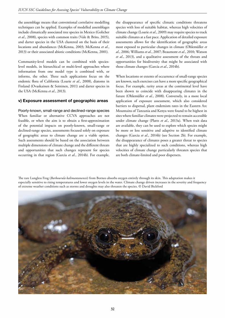
32

IUCN SSC Guidelines for Assessing Species’ Vulnerability to Climate Change

the assemblage means that conventional correlative modelling techniques can be applied. Examples of modelled assemblages include climatically associated tree species in Mexico (Golicher et al., 2008), species with common traits (Vale & Brito, 2015), and darter species in the USA clustered on the basis of their locations and abundances (McKenna, 2003; McKenna et al., 2013) or their associated abiotic conditions (McKenna, 2001).

Community-level models can be combined with species-level models, in hierarchical or multi-level approaches where information from one model type is combined with, or informs, the other. Three such applications focus on the endemic flora of California (Loarie et al., 2008), diatoms in Finland (Ovaskainen & Soininen, 2011) and darter species in the USA (McKenna et al., 2013).

v)Exposureassessmentofgeographicareas

Poorly-known, small-range and declined-range speciesWhen familiar or alternative CCVA approaches are not feasible, or when the aim is to obtain a first-approximation of the potential impacts on poorly-known, small-range or declined-range species, assessments focused solely on exposure of geographic areas to climate change are a viable option. Such assessments should be based on the association between multiple dimensions of climate change and the different threats and opportunities that such changes represent for species occurring in that region (Garcia et al., 2014b). For example,

the disappearance of specific climatic conditions threatens species with loss of suitable habitat, whereas high velocities of climate change (Loarie et al., 2009) may require species to track suitable climates at a fast pace. Application of detailed exposure assessments allows for the identification of geographic areas most exposed to particular changes in climate (Ohlemüller et al., 2006; Williams et al., 2007; Beaumont et al., 2010; Watson et al., 2013), and a qualitative assessment of the threats and opportunities for biodiversity that might be associated with those climate changes (Garcia et al., 2014b).

When locations or extents of occurrence of small-range species are known, such exercises can have a more specific geographical focus. For example, rarity areas at the continental level have been shown to coincide with disappearing climates in the future (Ohlemüller et al., 2008). Conversely, in a more local application of exposure assessment, which also considered barriers to dispersal, plant endemism rates in the Eastern Arc Mountains of Tanzania and Kenya were found to be highest in sites where familiar climates were projected to remain accessible under climate change (Platts et al., 2013a). When trait data are available, they can be used to explore which species might be more or less sensitive and adaptive to identified climate changes (Garcia et al., 2014b) (see Section 2b). For example, the disappearance of climates poses a greater threat to species that are highly specialized to such conditions, whereas high velocities of climate change particularly threaten species that are both climate-limited and poor dispersers.

32

The rare Lungless Frog (Barbourula kalimantanensis) from Borneo absorbs oxygen entirely through its skin. This adaptation makes it especially sensitive to rising temperatures and lower oxygen levels in the water. Climate change driven increases in the severity and frequency of extreme weather conditions such as storms and droughts may also threaten the species. © David Bickford

33

5.1.Selectingandusinginputdata

Section 4.1 (Steps 2–5) discussed ‘Carrying out your own CCVA’, including selecting appropriate spatial, taxonomic and temporal scales for meeting your CCVA objectives and considerations of the data needed to meet them. This section covers the extent and resolution of data needed to meet these objectives.

5.1.1Spatialextentandresolution

Spatial extent is the total area under consideration for a CCVA. If a specific area such as a country, subnational unit or site is specified as the objective of a CCVA, then that area will often form the spatial extent of the analysis. If the focal species’ vulnerability is not to be over-estimated, it is important to include areas that are contiguous with or close to the species’ present range and those that may become climatically suitable for the species in future.

When using many correlative modelling approaches, however, spatial extent should include at least the entirety of a focal species’ geographical distribution, thereby encompassing the full range of climatic conditions in which it currently occurs. Depending on the time frame, it may be necessary to include areas quite distant from the current distribution to identify future habitat. Including a large spatial extent is important, firstly, because if only parts of the distribution of a focal species are considered, estimates of niche characteristics such as niche breadth are likely to be underestimated and misrepresented, and are thus likely to result in overestimated vulnerability. Secondly, since the magnitude of projected climate changes is not uniform, some sites, countries and regions are projected to experience relatively limited changes, whereas others are projected to experience conditions unlike those found currently in any part of the given area today by the end (and in many cases the middle) of the 21st century. If the spatial extent is set to a limited part of the focal species’ range, assessments may overestimate species’ vulnerability. If that area is projected to contain only novel climates (i.e., with combinations of variables not found in the area today) then in the future it will appear unsuitable for all species currently present in the area, even though that combination of conditions may well occur currently outside the focal area. The correlative CCVA results are therefore likely to be an overestimation of species’ vulnerability and fail to account for influx of species not currently occurring in the focal area. If, however, the projected climate changes within the limited area considered are of smaller magnitude than those across the species’ range as a whole, then the assessment may underestimate vulnerability.

Spatial grain or resolution is relevant when a CCVA is to be performed using a modelling approach that requires gridded data, and refers to the area or linear dimension(s) of the grid cells used. The appropriate grain size will often be determined by the resolution of the available data such that the essential dataset with the coarsest resolution generally determines the limit to which grain size can be reduced. For example, whilst a digital elevation model may be available on a 50 m grid (i.e., 50 x 50 m), if species’ distribution data are recorded for a 1 km grid, (i.e., 1 x 1 km) then the latter is the finest practical grain size for most analyses.

Whilst a very fine grain (e.g., 10 m) might be used in principle, in practice a number of considerations will determine the appropriate resolution. Species’ distribution data may have been recorded as presence/absence in cells of a grid at a particular grain size or be derived from point records with limited spatial precision; the grid resolution or point precision then effectively determines the minimum grain size at which modelling can be performed. The scale of spatial heterogeneity in the region being considered will also influence the appropriate grain size; a coarser grain may present few problems in areas of relatively low spatial heterogeneity (e.g., flat terrain or uniform land-surface properties), whereas finer grains may be necessary in areas of higher spatial heterogeneity (e.g., topographically complex, varying land-surface properties).

In many cases the overall extent of the species’ range will impose a practical limit on the grain size because of the computational demands of finer grains. Moving from a 0·5° to a 30” grid increases by a factor of 3,600 the number of grid cells for which data must be stored and processed, and hence increases both computation time and memory requirements for modelling by at least this factor. Even if computation time scales only linearly, a model taking 1 second to fit at 0·5° will require 1 hour to fit at 30”, whilst if processing scales by the square of the data size, as it often does, then the 30” model will take 150 days to fit.

Additional issues need to be taken into account when adopting finer grains. Firstly, whereas the majority of the spatial patterns in a species’ distribution and abundance at grain sizes greater than ~20 km can generally be explained by bioclimatic variables alone (Luoto et al., 2007), at finer grains it will generally be necessary also to include non-climatic variables related to habitat availability (e.g., land cover, geology, soil type, hydrological features). At very fine grains, however, habitat is less important and microclimate becomes the dominant factor determining the distribution and abundance patterns of species

5.UsingCCVAsandinterpretingtheirresultsBrian Huntley, Wendy B. Foden, Adam Smith, Philip Platts, James Watson and Raquel A. Garcia

34

IUCN SSC Guidelines for Assessing Species’ Vulnerability to Climate Change

that experience the boundary-layer climate rather than the macroclimate (Gillingham et al., 2012a, 2012b). Furthermore, modelling such species at coarser grains can lead to a severe over-estimation of their vulnerability to climate change (Gillingham et al., 2012a).

In this context it is important to note that the interpolation of climatic variables performed to produce the finest grain datasets generally available assumes that grid cells are flat and uninfluenced by their neighbours. Even at the 30” grain of the WorldClim dataset it is arguable that topographic factors such as slope and aspect ought to have been taken into account. Already at this grain (0.855 km2 at the equator; 0.000126 km2 at the poles) the effect of insolation on temperature can be extremely important and is determined principally by slope and aspect. These topographic variables also influence drainage patterns, and hence the redistribution of precipitation that runs off rather than percolating into the soil. In many high-relief landscapes the shading effect of surrounding areas of higher elevation further impacts upon local temperatures, as do phenomena such as cold-air drainage and lake effects (see Bennie et al., 2008, 2010; Maclean et al., 2012; Hodgson et al.

For species occupying habitats with short vegetation, or the tops of forest canopies, models have been developed to estimate microclimatic conditions based on macroclimate records, taking into account topographic factors such as slope, aspect and shading by adjacent areas at higher elevation (Bennie et al., 2008, 2010). In principle such models might be extended to estimate microclimatic conditions under forest canopies where temperatures experienced by understorey species generally are cooler and humidity higher than in open areas (De Frenne et al., 2013; Hardwick et al., 2015). As a “rule of thumb”, such approaches ought to be applied to generate estimates of relevant microclimatic variables in any CCVA or other study that uses a grain size of ~1 km or less. In order to do so, however, it should be noted that a suitably fine-grained digital elevation model (DEM) will be required for the study area to enable estimation of the necessary topographic variables. It is also worth noting that at fine spatial scales, increased stochasticity in the data will mean that model performance may appear worse than when larger spatial scales are used.

5.1.2Timeframes

Temporal extent refers to the time frame under consideration (e.g., climate changes by 2050 or 2100). As discussed in Section 3 (Setting climate change vulnerability assessment goals and objectives), this will be informed by assessors’ needs, the biology (e.g., generation length) of focal taxa, and the length of the temporal time series of projected climatic data that are available (mostly to 2100 but some IPPC AR5 simulations extend to 2300).

Temporal resolution refers to the unit of time sampled within the temporal extent considered (e.g., daily, monthly, annual). A temporal resolution of less than annual will rarely be required

for a CCVA, as only a minority of species likely to be considered have a generation length of less than a year. Temporal resolution should not be confused with the period which relevant climatic variables may represent; the mean temperature of the warmest month of the year may, for example, be a relevant variable, for which an annual time series will enable a CCVA to be performed with annual temporal resolution.

5.1.3Climatedatasets

The choice of which projection(s) of future climatic conditions to use is one of the most important in CCVA (Snover et al., 2013). That decision in turn is influenced by four key questions: (i) which model(s) of the climate system should be used? (ii) which emissions scenario(s) are appropriate? (iii) which historical or baseline climate dataset is suitable? and (iv) which bioclimatic variables should be used?

5.1.3.1 General Circulation Models (GCMs)Choice of climate model should favour those most recently used and recommended by the IPCC (e.g., the latest IPCC Assessment Report), and that are either fully coupled atmosphere-ocean general circulation models (AOGCMs, e.g., HadCM3 (Gordon et al., 2000) or preferably earth system models (ESMs, e.g., HadGEM1 (Pope et al., 2007) that typically have improved representations of land-surface atmosphere interactions, as well as coupled simulations of terrestrial vegetation cover. Where the spatial extent of the planned CCVA is relatively limited, and especially in regions of complex topography, a Regional Climate Model (RCM (Morales et al., 2007), e.g., PRECIS) is likely to provide more accurate projections, provided that the boundary conditions used are from an appropriate AOGCM or ESM simulation, because RCMs operate mechanistically on horizontal resolutions of tens, rather than hundreds, of kilometres. The island of Madagascar, for example, is spanned by over 300 RCM squares (of side 55 km) but only a dozen or so squares at a typical GCM resolution.

The Coordinated Regional Climate Downscaling Experiment (CORDEX) has made available a series of regional datasets derived from RCM simulations. These are of continental scale and have a grain size of 0.44 DD (~55 km at the equator). Even regional models, however, are unable adequately to resolve fine-scale climatic variability across regions of high relief. A subsequent, non-mechanistic, downscaling step may therefore be desirable to recover fine-scale spatial variation at sub-RCM scales, as well as to remove model bias compared to the baseline climate data (see Section 5.1.3.5 (Understanding and preparing future climate scenarios). In most cases it will be preferable to carry out CCVA using equivalent projections from each of several (at least three) climate models. These models should be selected so as to encompass the range of uncertainty amongst models; choosing a number of models which each give projections close to the ensemble mean of all models included by the IPCC has little value, and simply increases the amount of computation required.

35

Having made assessments using each climate projection, the model outputs may then be combined into an ‘ensemble’ or mean which is generally regarded as the main output, while the various individual assessments provide an indication of the spread of potential values and hence of uncertainty in the results. Note that combining the climate model projections in an ensemble mean climate projection at the outset and then making a single assessment is inadvisable, because this will provide no insight into the range of uncertainty in outputs. Since different models may generate qualitatively different circulation patterns, it could also result in an ensemble mean climate projection that is mechanistically unrealistic or physically impossible. For example, a major atmospheric circulation feature, such as a persistent front, a jet stream or the path of monsoon winds, can be simulated by different models to occupy markedly different geographical locations, especially if a major topographic feature, such as a mountain range, ‘steers’ the feature to one side or the other of that feature. Taking a mean of two such contrasting simulations will tend to obliterate the spatial patterns in climatic variables associated with the circulation feature, such as the steep spatial gradient in temperature associated with a persistent front or the concentration of rainfall associated with the path of monsoon winds, resulting in mechanistically unrealistic mean climatic patterns. Doing so also can cover up year-to-year variance, which may be an important driver of vulnerability.

5.1.3.2 Emissions scenariosIt is tempting to advocate that greenhouse gas emissions scenarios should be selected to represent a plausible range of possible futures; alternatively, adoption of the precautionary principle might be advocated. In support of the latter

approach, the evidence of the past 25 years is that emissions have continued more or less along the worst case trajectory considered plausible by the IPCC in 1990 (Raupach et al., 2007). Hence it can be advocated that one should take the worst-case amongst plausible emissions scenarios (i.e., that corresponding more or less to ‘business-as-usual’) as the basis for performing a CCVA. Whilst some may argue that this is likely to exaggerate the problems faced by species and by biodiversity generally, improvements in climate models over the same period have not reduced the magnitude of disparities between climate changes projected by different models and under different emissions scenarios. Indeed, if anything the upper bounds on the range of uncertainty of future climate change magnitudes have increased (Stainforth et al., 2005). Add to that the acknowledged fact that a number of key positive feedbacks in the climate system, notably the effects of the snow-vegetation interaction on the snow-albedo feedback at higher latitudes, and the complex soil-moisture-vegetation-precipitation feedback in semi-arid areas such as the Sahel, are not adequately represented in current climate models, and the argument for adopting the precautionary principle when selecting plausible emissions scenarios to use when performing CCVAs is strong.

Whichever approach to selecting emissions scenarios is adopted, it is important that only potentially realistic scenarios such as those developed over the past ~25 years by the IPCC should be included. The Representative Concentration Pathway (RCP) scenarios used in the IPCC’s Fifth Assessment Report (IPCC, 2013a) should be favoured wherever possible over the older SRES scenarios used in the Fourth Assessment Report (IPCC, 2007b). The earlier IS92 and SA90 scenarios should generally no longer be used since evidence that emissions since 1990 have emerged as close to the highest ‘business as usual’ SA90 scenario means that the emissions range they consider is not realistic.

IPCC’s Fifth Assessment Report includes four trajectories for atmospheric emissions and radiative forcing in the 21st century: RCP 2.6, RCP 4.5, RCP 6 and RCP 8.5 (the forcing in W.m2 determines the number proceeding RCP). Most optimistically, RCP 2.6 assumes that greenhouse gas emissions are multilaterally reduced with immediate effect, such that atmospheric concentrations peak and decline by the year 2100, with the global mean temperature anomaly remaining below 2  °C relative to pre-industrial levels. Although technically feasible (Vuuren et al., 2011), this trajectory is unlikely given recent trends. The other scenarios project global mean temperature anomalies of up to ~5 °C by 2100. In terms of temperature anomaly, the closest SRES equivalents are B1 (RCP 4.5) and A1F1 (RCP 8.5) (Rogelj et al., 2012). If the precautionary principle is not adopted, then inclusion of at least three scenarios is recommended and two is regarded as the absolute minimum number to consider, in which case they should represent the overall range of plausible uncertainty about future emissions (i.e., a ‘high’ and a ‘low’ emissions scenario,

Clownfish (family: Pomacentridae) have close relationships with sea-anemones, relying on them for protection. Clownfish are believed to locate their particular host sea-anemone using a sense of smell, but laboratory experiments suggest that this sense may be impaired by more acidic ocean water. In addition, both clownfish and sea-anemones depend on coral reefs for habitat, and hence are threated indirectly by reef bleaching and ocean acidification impacts on them. © Flickr - Alfonso Gonzalez

5. Using CCVAs and interpreting their results

36

IUCN SSC Guidelines for Assessing Species’ Vulnerability to Climate Change

e.g., RCP8.5 and RCP4.5). If the precautionary principle is adopted, then RCP8.5 is recommended.

In contrast to working with climate models, it is almost always inappropriate to calculate any kind of ensemble mean of the CCVA results for two or more emissions scenarios. Instead, individual CCVAs should be made for alternative emissions scenarios so as to obtain insight into the uncertainty in the CCVA that relates to uncertainty about future emissions. There is a fundamental difference between this uncertainty related to unknowns about future human population growth, standards of living and global economic, energy and other policies, and the uncertainty related to different climate models, which arises from uncertainties in climate science, differences in model formulation and the need for simplification of systems by all models.

5.1.3.3 Historical (baseline) datasetsThe most widely used datasets representing baseline climate observations, as well as three satellite-derived rainfall datasets with potential for use, are shown in Table 8. Choice of dataset will depend upon the spatial extent and grain size at which the CCVA is to be performed, as discussed above under Section 5.1.1 (Spatial extent and resolution), as well as the most appropriate time period in relation to the period when species’ data were collected. In particular, where mean climatic

values for “custom” periods are required, the best available option is to use the 0·5° CRU TS3.22 dataset (Harris et al., 2014) of monthly means for 1901–2014, complemented, if appropriate, by rainfall and/or temperature data from one of the satellite-derived datasets (recent decades only). In the case of the datasets based on observed climate records from weather stations around the world, it is important to recognize that such stations are more sparsely distributed in the developing world, particularly in the tropics (e.g., Saharan and tropical Africa), and also are much sparser at higher elevations globally. Projections for such regions made using these baseline datasets are thus subject to greater uncertainty.

5.1.3.4 Bioclimatic variablesThe choice of bioclimatic variables used for a CCVA should be tailored to the focal species. Although there are very few species for which autecological studies have identified the precise bioclimatic variables that are important and/or their mechanisms of action (e.g., Pigott & Huntley, 1981), the general biological knowledge accumulated for a range of taxonomic groups and climatic regions, as well as the results from the many studies that have fitted species-climate envelope models of various types, provides a basis for an informed and intelligent choice of bioclimatic variables for most species. As a general observation, notwithstanding many studies in which it has been used, mean annual temperature is unlikely ever

Table 8. Examples of the most widely used and generally available climate datasets representing historical (baseline or recent past) climatic conditions.

Dataset name Spatial extent Temporal extent Spatial resolution Data available at: (URL)

Datasets using meteorological station data interpolated with respect to longitude, latitude and elevation

CRUCLv.2.1(Mitchellet al.,2004)

Europe 1961–90(30-yearmeans)

10minutes(~18.4x18.6km=342km2)*

Availableonrequest

CRUTSv.3.22(Harriset al.,2014)

Global 1901–2013(annualdata)

0.5degrees(~55x56km=3,077km2)*

http://www.cru.uea.ac.uk/cru/data/hrg/

WorldClim(Hijmanset al.,2005)

Global 1950–2000(periodmeans)

30seconds(~922x928m=0.855km2)*

http://www.worldclim.org/

Prism(Daly et al.,2002)

UnitedStates 1895–ongoing 30seconds(~922x928m=0.855km2)*

http://prism.oregonstate.edu/

Datasets using satellite remote-sensed data, usually processed through some form of model that often includes assimilation of data from meteorological stations

CHIRPSv2.0(Funket al.,2014)

50°S–50°N(Rainfallonly)

1981–present(daily,10-day,monthly&annualdata)

0.05degrees(~5.5x5.6km=30.8km2)

http://chg.geog.ucsb.edu/data/chirps/#plus7

MODISLandSurfaceTemperature/EmissivityGlobal

Global March2000–present(daily,8-day,monthly)

1kmto0.05degrees http://modisland.gsfc.nasa.gov/temp.html

TAMSAT/TARCATv2.0(Maidmentet al.,2014;Tarnavskyet al.,2014)

Africa(Rainfallonly)

1983–present(10-day,monthly&seasonaldata)

0.0375degrees(135seconds)(~4.15x4.17km=17.3km2)*

http://www.met.reading.ac.uk/~tamsat/cgi-bin/data/rfe.cgi?type=clim

TRMM/3B42 50°S–50°N(Rainfallonly)

March2000–present(daily,10-day,30-day)

0.25degrees(27.6x27.8km=769km2)

http://pmm.nasa.gov/data-access/downloads/trmm

*AverageneartheequatorCRU:ClimateResearchUnit

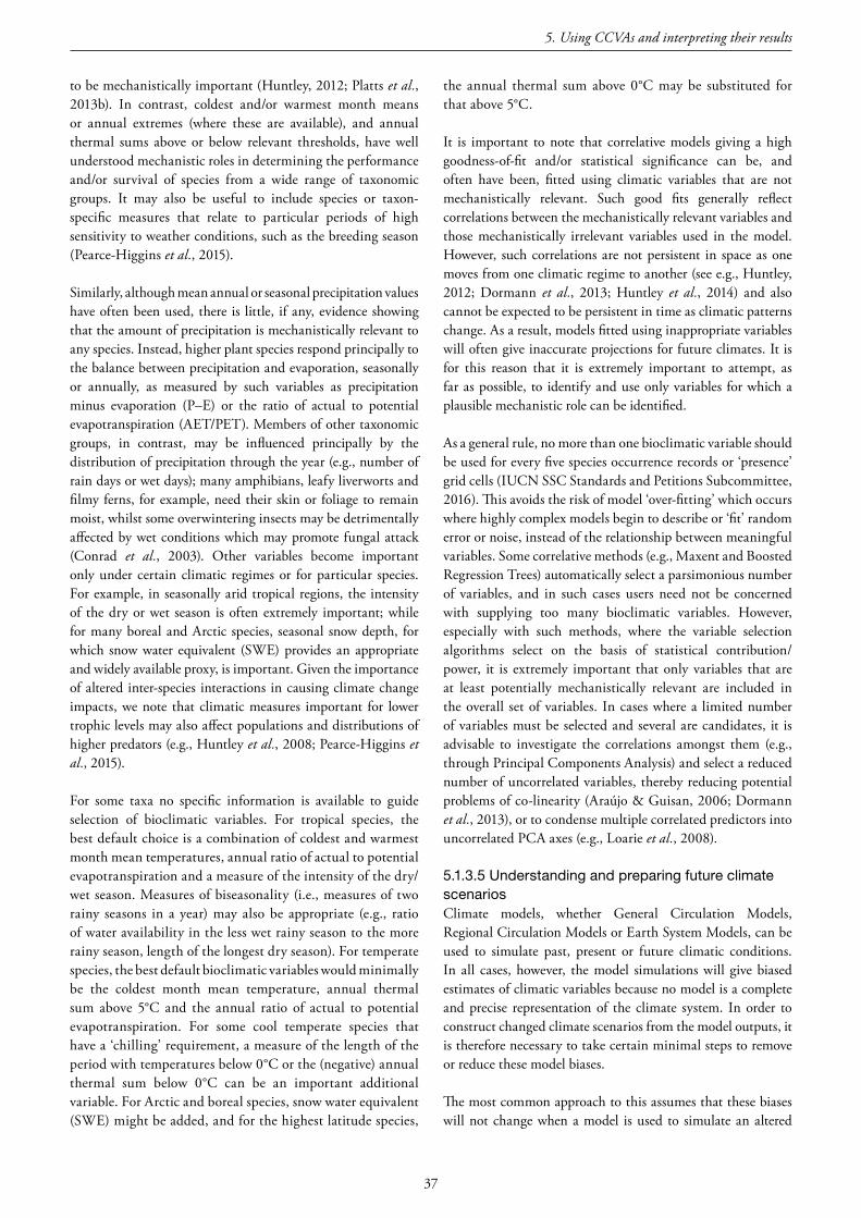
37

to be mechanistically important (Huntley, 2012; Platts et al., 2013b). In contrast, coldest and/or warmest month means or annual extremes (where these are available), and annual thermal sums above or below relevant thresholds, have well understood mechanistic roles in determining the performance and/or survival of species from a wide range of taxonomic groups. It may also be useful to include species or taxon-specific measures that relate to particular periods of high sensitivity to weather conditions, such as the breeding season (Pearce-Higgins et al., 2015).

Similarly, although mean annual or seasonal precipitation values have often been used, there is little, if any, evidence showing that the amount of precipitation is mechanistically relevant to any species. Instead, higher plant species respond principally to the balance between precipitation and evaporation, seasonally or annually, as measured by such variables as precipitation minus evaporation (P–E) or the ratio of actual to potential evapotranspiration (AET/PET). Members of other taxonomic groups, in contrast, may be influenced principally by the distribution of precipitation through the year (e.g., number of rain days or wet days); many amphibians, leafy liverworts and filmy ferns, for example, need their skin or foliage to remain moist, whilst some overwintering insects may be detrimentally affected by wet conditions which may promote fungal attack (Conrad et al., 2003). Other variables become important only under certain climatic regimes or for particular species. For example, in seasonally arid tropical regions, the intensity of the dry or wet season is often extremely important; while for many boreal and Arctic species, seasonal snow depth, for which snow water equivalent (SWE) provides an appropriate and widely available proxy, is important. Given the importance of altered inter-species interactions in causing climate change impacts, we note that climatic measures important for lower trophic levels may also affect populations and distributions of higher predators (e.g., Huntley et al., 2008; Pearce-Higgins et al., 2015).

For some taxa no specific information is available to guide selection of bioclimatic variables. For tropical species, the best default choice is a combination of coldest and warmest month mean temperatures, annual ratio of actual to potential evapotranspiration and a measure of the intensity of the dry/wet season. Measures of biseasonality (i.e., measures of two rainy seasons in a year) may also be appropriate (e.g., ratio of water availability in the less wet rainy season to the more rainy season, length of the longest dry season). For temperate species, the best default bioclimatic variables would minimally be the coldest month mean temperature, annual thermal sum above 5°C and the annual ratio of actual to potential evapotranspiration. For some cool temperate species that have a ‘chilling’ requirement, a measure of the length of the period with temperatures below 0°C or the (negative) annual thermal sum below 0°C can be an important additional variable. For Arctic and boreal species, snow water equivalent (SWE) might be added, and for the highest latitude species,

the annual thermal sum above 0°C may be substituted for that above 5°C.

It is important to note that correlative models giving a high goodness-of-fit and/or statistical significance can be, and often have been, fitted using climatic variables that are not mechanistically relevant. Such good fits generally reflect correlations between the mechanistically relevant variables and those mechanistically irrelevant variables used in the model. However, such correlations are not persistent in space as one moves from one climatic regime to another (see e.g., Huntley, 2012; Dormann et al., 2013; Huntley et al., 2014) and also cannot be expected to be persistent in time as climatic patterns change. As a result, models fitted using inappropriate variables will often give inaccurate projections for future climates. It is for this reason that it is extremely important to attempt, as far as possible, to identify and use only variables for which a plausible mechanistic role can be identified.

As a general rule, no more than one bioclimatic variable should be used for every five species occurrence records or ‘presence’ grid cells (IUCN SSC Standards and Petitions Subcommittee, 2016). This avoids the risk of model ‘over-fitting’ which occurs where highly complex models begin to describe or ‘fit’ random error or noise, instead of the relationship between meaningful variables. Some correlative methods (e.g., Maxent and Boosted Regression Trees) automatically select a parsimonious number of variables, and in such cases users need not be concerned with supplying too many bioclimatic variables. However, especially with such methods, where the variable selection algorithms select on the basis of statistical contribution/power, it is extremely important that only variables that are at least potentially mechanistically relevant are included in the overall set of variables. In cases where a limited number of variables must be selected and several are candidates, it is advisable to investigate the correlations amongst them (e.g., through Principal Components Analysis) and select a reduced number of uncorrelated variables, thereby reducing potential problems of co-linearity (Araújo & Guisan, 2006; Dormann et al., 2013), or to condense multiple correlated predictors into uncorrelated PCA axes (e.g., Loarie et al., 2008).

5.1.3.5 Understanding and preparing future climate scenariosClimate models, whether General Circulation Models, Regional Circulation Models or Earth System Models, can be used to simulate past, present or future climatic conditions. In all cases, however, the model simulations will give biased estimates of climatic variables because no model is a complete and precise representation of the climate system. In order to construct changed climate scenarios from the model outputs, it is therefore necessary to take certain minimal steps to remove or reduce these model biases.

The most common approach to this assumes that these biases will not change when a model is used to simulate an altered

5. Using CCVAs and interpreting their results

38

IUCN SSC Guidelines for Assessing Species’ Vulnerability to Climate Change

climate, and thus that any changes in conditions between a simulation by the model of present climate and of some altered climate will be robust. Changed climate scenarios for CCVA are thus best prepared by first using a model’s simulations of ‘present’ climate and of the altered climate of the selected time in the future to calculate the projected change or ‘anomalies’ in the climatic variables of interest. The ‘present’ in this case is that period covered by the chosen baseline climatic dataset. The changes, or anomalies, are then combined with the baseline dataset to obtain the required scenario of projected future climatic conditions. This ‘change-factor’ or ‘delta’ procedure for addressing biases in climate models when developing future climate scenarios for impact studies is well-established, and has been described in the literature in relation to the use of correlative models to project species’ potential future distributions on a number of occasions (e.g., Huntley et al., 1995, 2006, 2007) and also in relation to the generation of spatially downscaled climate change scenarios for various regions (e.g., Ramirez-Villegas & Jarvis, 2010; Tabor & Williams, 2010; Platts et al., 2015); it is discussed in more detail below.

Where they are available, users may prefer to select projections from lists of available climate datasets, but in doing so they should take care to establish that these have been constructed using appropriate methods. Alternatively, users may need to carry out the following steps themselves. In either case, it is important to understand the way that climate model outputs and baseline climatic data are used together to derive future climate scenarios.

Step 1. Calculate projected changes or anomalies from climate model outputs

To work out the degree of change projected by a climate model for a particular emissions scenario and time period, ‘anomalies’ or ‘change fields’ are calculated for each climatic variable of interest. Anomalies are generally calculated as the change between the model’s simulations of mean values of the climatic variable for ‘present’ (ideally the same period as is spanned by the baseline dataset to which the anomalies will be applied) and for the selected future time period, and are calculated for each climatic variable of interest and for all model grid cells relevant to the area of interest.

For temperature variables, anomalies are normally calculated as the arithmetical difference between future and ‘present’ values (i.e., additive anomalies; e.g., if a cell’s ‘present’ July mean temperature is 20 oC and the projected future value is 22oC, the anomaly will be +2oC). For precipitation-related variables such additive anomalies, although sometimes used (Tabor & Williams, 2010), generally are not recommended because climate models often have consistent ‘wet’ or ‘dry’ biases that result in large differences between models in absolute precipitation changes. This can readily be overcome by calculating anomalies as the ratio of the future to ‘present’ precipitation (i.e., multiplicative anomalies; e.g., if a cell’s

‘present’ mean January precipitation is simulated by two models to be 200 mm and 100 mm and the projected future simulated values are 300 mm and 150 mm, the anomaly will be 1.5 in both cases, whereas the additive anomalies would be 100 mm and 50 mm respectively). Problems arise if the projected future precipitation value is exactly zero; this is most readily overcome by adding a small amount (e.g., 1 mm) to both the ‘present’ and future values (Ramirez-Villegas & Jarvis, 2010; Platts et al., 2015). Because all climate models differ in their inherent biases, anomalies must be calculated separately for each model, as well as for each emissions scenario and time period being considered.

Step 2. Combine anomalies with baseline data to obtain future climate scenario

Having obtained the anomaly fields, the second step is to use these to calculate future climate scenarios by applying relevant anomalies to the baseline climatic data, either additively or multiplicatively, as described above. The selection of baseline climatic data at an appropriate grain was discussed above in Section 5.1.1 (Spatial extent and resolution). If, as is likely, the grain of the climate model, and hence of the derived anomalies, is coarser than that of the baseline dataset selected as appropriate for the CCVA, it is necessary to downscale the anomalies appropriately so as to obtain values to apply to the baseline data. Downscaling is usually performed by fitting spline surfaces to the anomalies in longitude-latitude space and using these surfaces to obtain interpolated values for the cells of the target grid. This approach is generally preferable to performing simple bi-linear or distance-weighted interpolation of the anomaly values for the climate model grid cells surrounding the target grid cell in the observed data, because of the generally large differences in grain and the inappropriateness of an assumption that anomalies are varying spatially in a simple linear fashion.

In terms of spatial downscaling, it is worth emphasizing that the change-factor method described here assumes temporal stasis in local spatial patterns of climatic variation, as inferred from the higher resolution baseline climatic data. For example, within an RCM grid square, and depending on the elevation contribution in the above interpolation, present patterns of temperature change with elevation, or of variation in precipitation arising from interactions between the orientation of mountain slopes and the prevailing wind direction, will be preserved. This assumption of temporal stasis of local spatial patterns is likely to be valid unless the GCM simulates changes (e.g., shifts in position, changes in strength, changes in orientation) in major features of the atmospheric and/or ocean circulation that strongly influence the climate of the region of interest. Even in such cases, however, until such time as global simulations of climate are available with a spatial resolution as high as or higher than that achieved by current RCMs, this assumption generally represents the most practical and pragmatic approach.

39

In regions with sufficiently dense observational time-series of climatic data, however, an alternative to change-factor downscaling is directly to correlate RCM outputs with local climatic conditions over time (statistical downscaling), and to use those relationships to project future fine-scale changes, correcting where appropriate for scenario-based changes in land-surface feedbacks (e.g. cloud base shifting upslope due to deforestation) or in the microclimatic regulation provided by vegetation or snow cover. Such statistical downscaling relies upon an assumption that the relationships between fine-scale climatology and features of the climate system at coarser resolution will persist under changed general climatic conditions; this is both untested and unlikely.

5.1.4Speciesdistributiondata

For CCVA approaches that rely heavily on occurrence records for characterizing species’ climatic tolerances (i.e., correlative and mechanistic niche modelling approaches), it is particularly important that these data are of good quality (IUCN SSC Standards and Petitions Subcommittee, 2016). Occurrence records should have accurate locations, the acceptable spatial precision of which will be determined by the spatial resolution at which the CCVA is to be performed (e.g., accurate locations with a precision of ≤~100m will be required for an analysis at a resolution of 1 km2). For best accuracy, the projection (e.g., WGS84) should be specified. Identifying spatially inaccurate records is often difficult, but two procedures can help. Firstly, mapping the records (in a GIS or Google Earth) will allow anomalous or outlying records to be identified and investigated (Pearson, 2007). Comparison with the expert-mapped distribution polygons (see Table 6 for examples of sources) or published maps, where available, may also be helpful, but care needs to be taken that accurate records are not removed unnecessarily, simply because they are located outside of such distribution polygons. Where available, good quality survey or atlas data, or a set of well-validated records, is likely to be more accurate and useful than an expert-based polygon. Secondly, where records give altitude as well as longitude and latitude, overlaying the longitude-latitude location onto a high-resolution DEM allows the consistency of the altitude to be checked; records for which the match in altitude is unacceptably poor can then be investigated or rejected.

Further uncertainty can be introduced into analyses if occurrence data are spatially biased. Many datasets, for example, will have higher densities of records from areas closer to human settlements or roads. This can introduce important biases with respect to the sampling of environmental space that will result in inaccurate models. However, if information on such sampling biases can be collected, then appropriate selection of absence data can allow modelling approaches to take some account of such biases (see Phillips et al., 2009). When this is not possible, other methods such as thinning (subsampling records) in geographic space (Aiello-Lammens et al., 2015) or environmental space (Varela et al., 2014), or

weighting presences by the inverse of their local density (Stolar & Nielsen, 2015) can be used to remove bias.

Identification uncertainty should be minimized. For less well-known or difficult-to-identify taxa, occurrence records should ideally be associated with vouchered specimens or, if appropriate, photographs that have been identified by relevant taxonomic experts, although modelling approaches increasingly allow uncertainty in record identification to be accounted for (Johnston et al., 2015). Data from large distribution databases (e.g., GBIF, HerpNET) may be used, but only with caution and following careful review for accuracy, coverage and sampling intensity (IUCN SSC Standards and Petitions Subcommittee, 2016). Although concern is sometimes expressed about the validity of records derived from citizen science approaches (e.g., e-Bird, BirdTrack, SABAP), in practice such schemes often provide the only practicable manner to obtain large-scale and extensive biological recording data, and include inbuilt verification mechanisms to ensure that unusual records are vetted by experienced recorders and verifiers. Such data have underpinned the majority of assessments of distribution and projected range change for many bird species (Huntley et al., 2008).

Further discussion on this topic is presented below inSection 6.1 (Uncertainty from species’ distribution andabundancedata).

5.1.5Speciestraitdata

There is growing recognition and understanding of the role that species’ biological characteristics play in exacerbating or mitigating sensitivity and adaptive capacity to climate change (Jiguet et al., 2007; Dawson et al., 2011; Nicotra et al., 2015). These include traits relating to species physiology, demography and ecology (Keith et al., 2008; Visser, 2008; Williams et al., 2008). Studies examining associations between biological traits and climate change-driven changes in population abundance, extinction risk and range shifts for a range of taxa contribute to a growing knowledge base (e.g., Cardillo et al., 2008; Murray et al., 2009; Thaxter et al., 2010; Angert et al., 2011; Newbold et al., 2013; Chessman, 2013; Pearson et al., 2014a; Estrada et al., 2015). These trait associations provide the basis for using traits for CCVA, and they present, at this stage, one of the few ways of accounting for the multiple pathways in which species may be impacted by climate change. Because they require ecological knowledge without strong statistical and modelling expertise, they are being adopted by many conservation organizations, particularly as it is possible to make assessments for large numbers of species relatively rapidly. A number of recent CCVAs have adopted a trait-based approach to assessing species’ vulnerability to climate change at either regional (Gardali et al., 2012; Trivino et al., 2013) or global (Foden et al., 2013) scales. We discuss the application of the approach, as well as some of its challenges and uncertainties, below, and in Section 6.5 (Uncertainty from biological trait and demographic data).

5. Using CCVAs and interpreting their results

40

IUCN SSC Guidelines for Assessing Species’ Vulnerability to Climate Change

5.1.5.1 Trait selectionTo date, selection of traits for both trait-based and mechanistic models has been largely expert-based, drawing on a priori assumptions about the mechanisms by which focal species are likely to be impacted. An example of a framework for guiding such trait selection is shown in Table 9, and examples

of the types of traits used in five recent trait-based CCVAs are shown in Table 10. Since this expert-based approach may introduce certain biases (Burgman et al., 2011), particularly in combination with the omissions of certain traits due to the realities of data availability and collection, we encourage users to document the rationales for their trait choices, desired

Table 9. Trait categories associated with species’ heightened sensitivity and low adaptive capacity to climate change(fromFodenet al.,(2013)andEstradaet al. (2016)).Assessorsmaychoose,fortheirfocalspecies,theoneormoretraitsthatdescribeeachcategory(e.g.,underD,forcorals,usersmightselect“susceptibletobleaching”).

SENSITIVITY

A. Specialized habitat and/or microhabitat requirementsAsclimatechange-drivenenvironmentalchangesunfold,speciesthatarelesstightlycoupledtospecificconditionsandrequirementsarelikelytobemoreresilientbecausetheywillhaveawiderrangeofhabitatandmicrohabitatoptionsavailabletothem.Sensitivityisfurtherincreasedforspecieswithseverallifestages,eachrequiringdifferenthabitatsormicrohabitats(e.g.,water-dependentlarvalamphibians).Wenote,however,thatthisdoesnotholdinallcases,andextremespecializationmayallowsomespeciestoescapethefullimpactsofclimatechangeexposure(e.g.,deepseafishes).

B. Environmental tolerances or thresholds (at any life stage) that are likely to be exceeded due to climate changeSpecieswithphysiologicaltolerancesthataretightlycoupledtospecificenvironmentalconditions(e.g.,temperatureorprecipitationregimes,waterpHoroxygenlevels)arelikelytobeparticularlysensitivetoclimatechanges(e.g.,tropicalectotherms)(Deutschet al.,2008;McCain,2009).However,evenspecieswithbroadenvironmentaltolerancesmayalreadybeclosetothresholdsbeyondwhichphysiologicalfunctionquicklybreaksdown(e.g.,drought-tolerantdesertplants(Foden et al.,2007)).

C. Dependence on environmental triggers that are likely to be disrupted by climate changeManyspeciesrelyonenvironmentaltriggersorcuestoinitiatelifestages(e.g.,migration,breeding,egglaying,seedgermination,hibernationandspringemergence).Whilecuessuchasdaylengthandlunarcycleswillbeunaffectedbyclimatechange,thosedrivenbyclimateandseasonmayalterinboththeirtimingandmagnitude,leadingtoasynchronyanduncouplingwithenvironmentalfactors(Thackerayet al.,2010)(e.g.,mismatchesbetweenadvancingspringfoodavailabilitypeaksandhatchingdates(Bothet al.,2006)).Climatechangesensitivityislikelytobecompoundedwhendifferentsexesorlifestagesrelyondifferentcues.

D. Dependence on interspecific interactions that are likely to be disrupted by climate changeClimatechange-drivenalterationsinspecies’ranges,phenologiesandrelativeabundancesmayaffecttheirbeneficialinter-specificinteractions(e.g.,withprey,pollinators,hostsandsymbionts)and/orthosethatmaycausedeclines(e.g.,withpredators,competitors,pathogensandparasites).Speciesarelikelytobeparticularlysensitivetoclimatechangeif,forexample,theyarehighlydependentononeorfewspecificresourcespeciesandareunlikelytobeabletosubstitutetheseforotherspecies(Mølleret al.,2011).

E. RarityTheinherentvulnerabilityofsmallpopulationstoAlleeeffectsandcatastrophicevents,aswellastheirgenerallyreducedcapacitytorecoverquicklyfollowinglocalextinctionevents,suggestthatmanyrarespecieswillbemoresensitivetoclimatechangethancommonspecies.Rarespeciesincludethosewithverysmallpopulationsizes,aswellasthosethatmaybelocallyabundantbutaregeographicallyhighlyrestricted.

LOW ADAPTIVE CAPACITY

F. Poor dispersal ability: Intrinsicdispersallimitations:Specieswithlowdispersalratesorlowpotentialforlongdistancedispersal(e.g.,landsnails,antandraindropsplash-dispersedplants)havelowestadaptivecapacitysincetheyareunlikelytobeabletokeepupwithashiftingclimateenvelope.Estradaet al.(2016)outlineaframeworkhighlightinghowfourkeyrange-shiftprocessesareaffectedbyseventraittypes,namely(withtraitsinbrackets):(i)emigration(sitefidelity);(ii)movement(movementability);(iii)establishment(avoidanceofsmallpopulationeffects,persistenceunderunfavourableconditions);and(iv)proliferation(reproductivestrategy;ecologicalgeneralizationandcompetitiveability(thesethreetraitsapplytoprocesses(iii)and(iv))).

Extrinsicdispersallimitations:Evenwherespeciesareintrinsicallycapableoflongdistanceorrapiddispersal,movementand/orsuccessfulcolonizationmaybereducedbylowpermeabilityorphysicalbarriersalongdispersalroutes.Theseincludenaturalbarriers(e.g.,oceansorriversforterrestrialspecies),anthropogenicbarriers(e.g.,damsforfreshwaterspecies)andunsuitablehabitatsorconditions(e.g.,oceancurrentsandtemperaturegradientsformarinespecies).Speciesforwhichnosuitablehabitator‘climatespace’islikelytoremain(e.g.,Arcticice-dependentspecies)mayalsobeconsideredinthistraitset.

G. Poor evolvability:Species’potentialforrapidgeneticchangewilldeterminewhetherevolutionaryadaptationcanresultataratesufficienttokeepupwithclimatechange-drivenchangestotheirenvironments.Specieswithlowgeneticdiversity,oftenindicatedbyrecentbottlenecksinpopulationnumbers,generallyexhibitlowerrangesofbothphenotypicandgenotypicvariation.Asaresult,suchspeciestendtohavefewernovelcharacteristicsthatcouldfacilitateadaptationtothenewclimaticconditions.

Sincedirectmeasuresofspecies’geneticdiversityarefew,proxymeasuresofevolvabilitysuchasthoserelatingtoreproductiveratesandoutputs,andhencetherateatwhichadvantageousnovelgenotypescouldaccumulateinpopulationsandspecies(Chevin et al.,2010),maybeuseful.Evidencesuggeststhatevolutionaryadaptationispossibleinrelativelyshorttimeframes(e.g.,5to30years(Bradshaw&Holzapfel,2006))butformostspecieswithlonggenerationlengths(e.g.,largeanimalsandmanyperennialplants),thisislikelytobetooslowtohaveanyseriousminimizingeffectonclimatechangeimpacts.

41

traits or mechanisms that were omitted, and where possible, to account for uncertainty in trait choice assessments through sensitivity analyses.

A key requirement in order to implement the trait-based approach is a database of species traits. For many taxonomic groups, such information is increasingly being collated, and may be empirically available from various data sources and organizations (see Table 6 and Section 4.1, Step 3 (Species trait data)). However, for many species, particularly for less-well studied taxa, such information may be lacking, and obtaining it must therefore rely upon an expert-based assessment, or potentially, the use of data from similar species. This flexibility makes the use of trait-based assessments attractive, as they can be conducted for any species and location given either a database of traits, or a number of species experts.

5.1.5.2 Trait threshold selectionQuantifying thresholds for categorizing the climate change vulnerability associated with each selected trait poses a major challenge to most trait-based methods. Thresholds of concern are clear for some traits (e.g., confined to a small island), but since most traits are described by continuous variables (e.g., body mass, fecundity, degree of habitat specialization), users must infer such thresholds. In rare cases, empirical studies are available to inform robust estimates of such thresholds (e.g., established growth performance curves and thermal extreme tolerances for Australian Drosophila (Overgaard et al., 2014)), but for most, users must make subjective choices based on their own observations, ecological understanding or even arbitrarily (e.g., the 25% worst-affected species, (Foden et al., 2013)). These challenges highlight the need for more empirical studies on species’ physiological limits.

5.1.5.3 Trait scoringTrait-based assessments to date have tended to quantify the per-species climate change vulnerability associated for each trait in one of three ways. Species have been assigned scores for each trait (e.g., from -1 to 1 (Bagne et al., 2011), 1 to 3 (Gardali et al., 2012), or 0–3 (Thomas et al., 2011), ordinal categories (e.g., “High/Medium/Low” (Chin et al., 2010) or “High/Low” (Foden et al., 2013)); or ranks (e.g., based on a hierarchical decision framework (Smith et al., 2016)).

i) To date little attention has been devoted toward scoring systems and the manner in which scores are combined (Willis et al., 2015), but these have important consequences for overall outcomes of TVA. A preliminary series of “best practices” for developing a scoring system includes these aspects:

ii) The number of graduations in the scoring system should reflect the amount of trait information available. For example, a finer scale (e.g., 0 to 10) allows for more nuanced distinction between trait states than a coarser scale (e.g., high/medium/low). Although it is conceptually easier to populate a scoring system with fewer graduations, coarser scales generally require more concerted thought about critical thresholds because the distinction between any given pair of scores is greater (e.g., on a zero-to-ten point system there is less relative difference between a score of 6 versus 7, whereas on a 3-point low-medium-high scale there is much greater distinction between “high” and “medium” or “medium” and “low”). Regardless of the scoring system, assessors should clearly document selected trait thresholds and provide justifications where possible.

iii) The scoring system should include a “neutral” score above/below which climate change is expected to be

Table 10. Examples of the traits considered by five trait-based CCVAs (adaptedfromWilliset al.,2015).

(Fodenet al.,2013)

(Garnettet al.,2013)

(Gardaliet al.,2012)

(Thomaset al.,2011)

(Grahamet al.,2011)

Habitatspecialization X X X X

Dietaryspecialization X X

Environmental/climatictolerance X X X

Inter-specificinteractionsaffected X X

Sensitivetoenvironmentaltriggers X

Rarity X X X

Dispersal X X

Evolvability X

Exposure X X X X

Reproductive/recruitmentcapacity X X X

Migratorystatus X

Otherthreats X

Bodysize X

Brainsize X

5. Using CCVAs and interpreting their results

42

IUCN SSC Guidelines for Assessing Species’ Vulnerability to Climate Change

harmful/beneficial to a species. Though climate change promises to cause large-scale disruption of species’ ecologies, not all effects will necessarily be negative; some species will benefit. Thus, it is important to reflect this potential in a scoring system and avoid assuming climate change will have only negative impacts. Even if no species in an assessment will actually benefit or be unaffected by climate change, neutral scores serve as a mental benchmark to anchor scores to a meaningful state (a state of no effect). They also allow for easier comparison between studies since a neutral score serves as a common denominator between different scoring systems. Inclusion of neutral scores is considered standard practice in fields where score-based systems are used as a basis for analysis (Ragin & Becker, 1992).

iv) Assessors should collect and store data in forms that make re-assessment possible should the understanding of climate change mechanisms underpinning the trait threshold selection change. Climate science and vulnerability assessment are rapidly-advancing fields; even though decisions are being made that are relevant to time periods many decades in the future, our understanding of consequences of climate change progresses every year. Thus it is very likely that an active management program will need to update its assessment as time progresses (and our knowledge of what climate and species may do becomes greater).

v) Assessors should include measures of confidence in each trait score (e.g., Bagne et al., 2011; Thomas et al., 2011; Gardali et al., 2012).

5.1.5.4 Calculating overall measures of vulnerabilityBefore combining trait scores into overall measures of climate change vulnerability, many authors have weighted the scores, either by expert judgement of trait importance (e.g., Graham et al., 2011; Gardali et al., 2012; Young et al., 2012) or according to confidence in score accuracy (e.g., Thomas et al., 2011). The resulting scores are then typically combined in one of two ways. The final score may be derived computationally (e.g., through additive (Bagne et al., 2011; Graham et al., 2011) or multiplicative

(Gardali et al., 2012) rules; see below) in which case the overall CCVA output may be scores and, often resulting from these, fall into overall vulnerability categories (e.g., Young et al., 2012) or ranks. Overall scores may also be reached through a rule-based logic framework which typically assigns species into overall vulnerability categories (e.g., Chin et al., 2010; Bagne et al., 2011; Foden et al., 2013). We encourage users to carry out sensitivity analyses to identify the uncertainty potentially introduced by their selected scoring system.

Score-combining systems have received almost no attention in the CCVA literature even though, like scoring systems, they have a direct impact on the final outcome of an assessment (Willis et al., 2015). In general, there are two “levels” of scoring rules, one used to combine scores within a module (reflecting, for example, exposure, sensitivity, or adaptive capacity) and another across modules (combining exposure, sensitivity, and adaptive capacity). Combining rules reflect how traits interact to convey overall vulnerability. Though there are many ways to combine scores computationally, we review here two relatively common and simple rules based on addition and multiplication.

Additive rules (score #1 + score #2 + score #3 + …) reflect situations where traits do not interact and can stand in for one another to enhance vulnerability or counter one another to reduce vulnerability. For example, a plant species’ sensitivity might be reflected by scores for two traits, one reflecting the lethal effects of high temperature on pollen and another reflecting the need for low winter temperatures necessary for seed stratification to break dormancy in the spring. Using a summation rule assumes traits can substitute for one another to confer the same amount of sensitivity to climate change (e.g., the species could have the same sensitivity regardless of whether it was sensitive to high temperatures or lack of low temperatures). Mathematically, summation rules retain symmetry around neutral scores (e.g., on a 7-point scale from -2 to 2, with 0 as the neutral score, adding two scores yields a new scale from -4 to 4 with 0 still being neutral). In this context a “mean” rule that averages across scores has the

This biodiversity conservation workshop in far northern Queensland included facilitated discussions in small groups about the challenges, opportunities and strategies for biodiversity conservation in the Wet Tropics in the light of the latest climate science. Researchers, local technical experts and experienced members from conservation based community groups participated in the discussions. © Terrain NRM

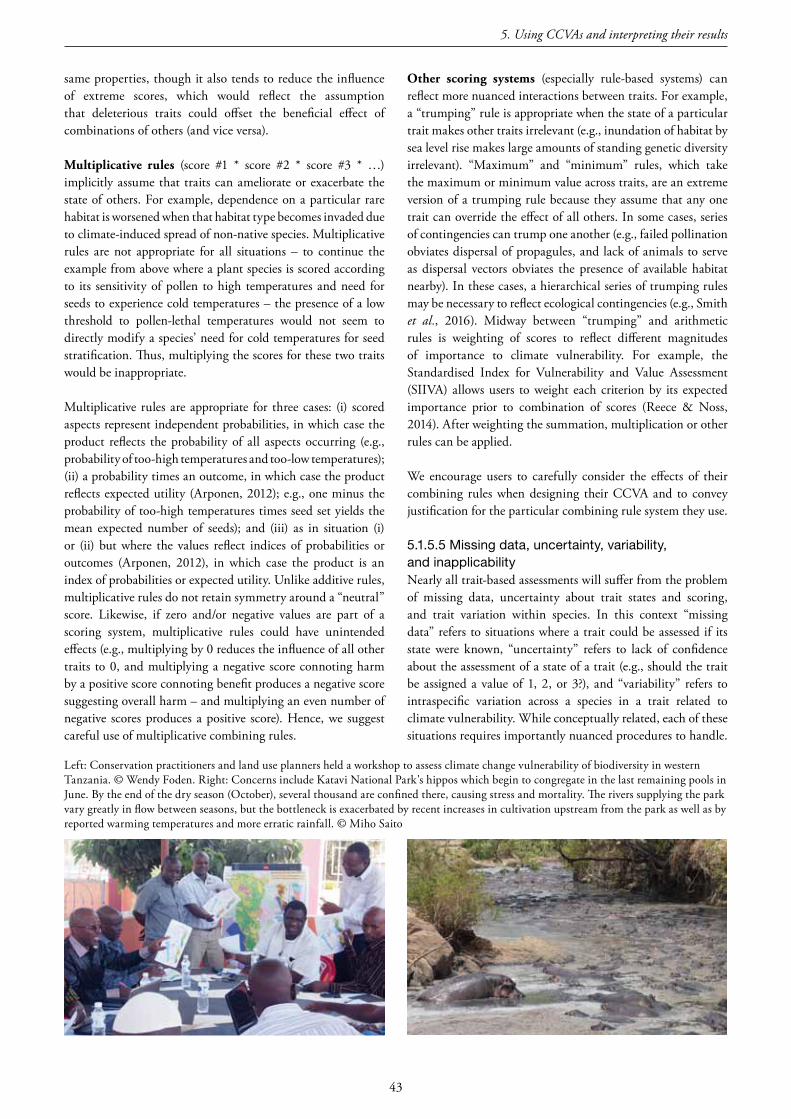
43

same properties, though it also tends to reduce the influence of extreme scores, which would reflect the assumption that deleterious traits could offset the beneficial effect of combinations of others (and vice versa).

Multiplicative rules (score #1 * score #2 * score #3 * …) implicitly assume that traits can ameliorate or exacerbate the state of others. For example, dependence on a particular rare habitat is worsened when that habitat type becomes invaded due to climate-induced spread of non-native species. Multiplicative rules are not appropriate for all situations – to continue the example from above where a plant species is scored according to its sensitivity of pollen to high temperatures and need for seeds to experience cold temperatures – the presence of a low threshold to pollen-lethal temperatures would not seem to directly modify a species’ need for cold temperatures for seed stratification. Thus, multiplying the scores for these two traits would be inappropriate.

Multiplicative rules are appropriate for three cases: (i) scored aspects represent independent probabilities, in which case the product reflects the probability of all aspects occurring (e.g., probability of too-high temperatures and too-low temperatures); (ii) a probability times an outcome, in which case the product reflects expected utility (Arponen, 2012); e.g., one minus the probability of too-high temperatures times seed set yields the mean expected number of seeds); and (iii) as in situation (i) or (ii) but where the values reflect indices of probabilities or outcomes (Arponen, 2012), in which case the product is an index of probabilities or expected utility. Unlike additive rules, multiplicative rules do not retain symmetry around a “neutral” score. Likewise, if zero and/or negative values are part of a scoring system, multiplicative rules could have unintended effects (e.g., multiplying by 0 reduces the influence of all other traits to 0, and multiplying a negative score connoting harm by a positive score connoting benefit produces a negative score suggesting overall harm – and multiplying an even number of negative scores produces a positive score). Hence, we suggest careful use of multiplicative combining rules.

Other scoring systems (especially rule-based systems) can reflect more nuanced interactions between traits. For example, a “trumping” rule is appropriate when the state of a particular trait makes other traits irrelevant (e.g., inundation of habitat by sea level rise makes large amounts of standing genetic diversity irrelevant). “Maximum” and “minimum” rules, which take the maximum or minimum value across traits, are an extreme version of a trumping rule because they assume that any one trait can override the effect of all others. In some cases, series of contingencies can trump one another (e.g., failed pollination obviates dispersal of propagules, and lack of animals to serve as dispersal vectors obviates the presence of available habitat nearby). In these cases, a hierarchical series of trumping rules may be necessary to reflect ecological contingencies (e.g., Smith et al., 2016). Midway between “trumping” and arithmetic rules is weighting of scores to reflect different magnitudes of importance to climate vulnerability. For example, the Standardised Index for Vulnerability and Value Assessment (SIIVA) allows users to weight each criterion by its expected importance prior to combination of scores (Reece & Noss, 2014). After weighting the summation, multiplication or other rules can be applied.

We encourage users to carefully consider the effects of their combining rules when designing their CCVA and to convey justification for the particular combining rule system they use.

5.1.5.5 Missing data, uncertainty, variability, and inapplicabilityNearly all trait-based assessments will suffer from the problem of missing data, uncertainty about trait states and scoring, and trait variation within species. In this context “missing data” refers to situations where a trait could be assessed if its state were known, “uncertainty” refers to lack of confidence about the assessment of a state of a trait (e.g., should the trait be assigned a value of 1, 2, or 3?), and “variability” refers to intraspecific variation across a species in a trait related to climate vulnerability. While conceptually related, each of these situations requires importantly nuanced procedures to handle.

5. Using CCVAs and interpreting their results

Left: Conservation practitioners and land use planners held a workshop to assess climate change vulnerability of biodiversity in western Tanzania. © Wendy Foden. Right: Concerns include Katavi National Park's hippos which begin to congregate in the last remaining pools in June. By the end of the dry season (October), several thousand are confined there, causing stress and mortality. The rivers supplying the park vary greatly in flow between seasons, but the bottleneck is exacerbated by recent increases in cultivation upstream from the park as well as by reported warming temperatures and more erratic rainfall. © Miho Saito

44

IUCN SSC Guidelines for Assessing Species’ Vulnerability to Climate Change

Missing data can be imputed (e.g., Schrodt et al., 2015) or replaced with targeted research. Nonetheless, there will remain situations in which trait states cannot be assigned. In this case, one option is to assign a particular score to missing values (e.g., a “no effect” score; Young et al., 2015). However, this implicitly makes an assumption about the strategy by which uncertainty is managed by the users of the CCVA. For example, assigning a “no effect” score for missing cases will tend to down-weight the final scores of species for which little is known (Anacker et al., 2013). In turn, this can have profound effects on the overall assessment of vulnerability across species (e.g., Platts et al., 2014). Another approach is to calculate overall vulnerability multiple times assuming different scores for missing data each time (e.g., reflecting benefit, no effect, or harm from climate change; Smith et al., 2016) and report the results as a range. A third option is to standardise scores within a module by, for example, dividing by the maximum possible score for each species; Reece & Noss, 2014). In this way missing scores become non-influential on the final outcome.

Missing data is just one aspect that contributes to uncertainty; other causes of uncertainty include lack of confidence about the state of a trait (versus complete lack of knowledge), difficulty in determining thresholds (i.e., assigning the appropriate score to a trait state), and conflicting accounts of trait states, amongst other causes. Again, several approaches have been used to address uncertainty, including independent assessment by multiple experts (i.e., a Delphi-like system; Runge et al., 2011) or assigning a range of scores. The CCVA can then be analysed multiple times using, for example, “optimistic” or “pessimistic” values of scores (e.g., Foden et al., 2013) or using Monte Carlo randomization (Reece & Noss, 2014). Another alternative is to design a separate “information availability” module which reflects completeness of knowledge about each species (Benscoter et al., 2013). Regardless, in most cases uncertainty should be reflected in the vulnerability assessment as a separate aspect (e.g., as a separate score – e.g., Moyle et al., 2013) – or as error bars – e.g., Benscoter et al., 2013 – or as distinct

optimistic or pessimistic “scenarios” – e.g., Foden et al., 2013; Smith et al., 2016. Some trait-based assessments weight final scores by uncertainty by, for example, assuming species with more uncertainty around their scoring are inherently of lower priority (e.g., Thomas et al., 2011; Shoo et al., 2013), which in this case is directly contradictory to the precautionary principle. Hence, we advise reporting uncertainty separately from “mean” (expected) vulnerability.

Variability in traits within species is similar to –yet importantly distinct from– uncertainty about traits (cf. Lehmann & Rillig, 2014a). Intraspecific variation is probably the rule rather than exception, yet trait-based (and other) approaches often assume that species act as homogenous units in response to climate change. Indeed, intraspecific variation can confer greater vulnerability to climatic variation if it reflects local adaptation (e.g., Valladares et al., 2014) or less vulnerability if it reflects ability to adapt genetically or through phenotypic plasticity (Avolio & Smith, 2013). Regardless, assigning a single score to an intraspecifically-varying trait ignores this important aspect of vulnerability. In this case the most appropriate practice would be to assign a range of values and calculate overall vulnerability multiple times to reflect intraspecific variation in traits. Alternatively, “variation in trait” can be treated as a trait itself to indicate increased/decreased vulnerability as a result of variation in the given trait.

In a related vein, some traits may be inapplicable for some species but applicable to others, a situation likely to arise when large suites of taxonomically diverse species are evaluated (e.g., Foden et al., 2013). For example, stream discharge rate is highly relevant to lotic fish but not to most birds. One option is to design separate CCVAs for each suite of species (e.g., Foden et al., 2013 evaluated corals, birds, and amphibians separately), but in some situations comparing vulnerability of disparate suites of species (e.g., in the same management unit) is desirable. In this context some of the methods used to handle missing data can be used (especially standardization). When there is

Leatherback Turtles (Dermochelys coriacea), already a critically endangered species, are being impacted by rising beach sand temperatures. At higher temperatures their buried eggs hatch a disproportionately high proportion of female turtles, leading to populations with strongly skewed sex ratios. Their nests and nesting habitat are also threatened by rising sea levels and increases in storm activity. Left: © Roderic Mast / Oceanic Society. Right: © Brian Hutchinson

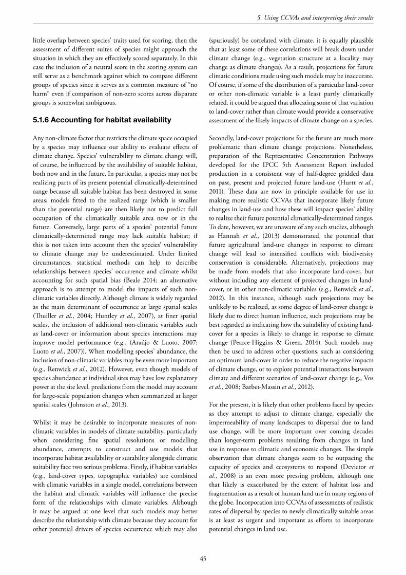
45

little overlap between species’ traits used for scoring, then the assessment of different suites of species might approach the situation in which they are effectively scored separately. In this case the inclusion of a neutral score in the scoring system can still serve as a benchmark against which to compare different groups of species since it serves as a common measure of “no harm” even if comparison of non-zero scores across disparate groups is somewhat ambiguous.

5.1.6Accountingforhabitatavailability

Any non-climate factor that restricts the climate space occupied by a species may influence our ability to evaluate effects of climate change. Species’ vulnerability to climate change will, of course, be influenced by the availability of suitable habitat, both now and in the future. In particular, a species may not be realizing parts of its present potential climatically-determined range because all suitable habitat has been destroyed in some areas; models fitted to the realized range (which is smaller than the potential range) are then likely not to predict full occupation of the climatically suitable area now or in the future. Conversely, large parts of a species’ potential future climatically-determined range may lack suitable habitat; if this is not taken into account then the species’ vulnerability to climate change may be underestimated. Under limited circumstances, statistical methods can help to describe relationships between species’ occurrence and climate whilst accounting for such spatial bias (Beale 2014; an alternative approach is to attempt to model the impacts of such non-climatic variables directly. Although climate is widely regarded as the main determinant of occurrence at large spatial scales (Thuiller et al., 2004; Huntley et al., 2007), at finer spatial scales, the inclusion of additional non-climatic variables such as land-cover or information about species interactions may improve model performance (e.g., (Araújo & Luoto, 2007; Luoto et al., 2007)). When modelling species’ abundance, the inclusion of non-climatic variables may be even more important (e.g., Renwick et al., 2012). However, even though models of species abundance at individual sites may have low explanatory power at the site level, predictions from the model may account for large-scale population changes when summarized at larger spatial scales (Johnston et al., 2013).

Whilst it may be desirable to incorporate measures of non-climatic variables in models of climate suitability, particularly when considering fine spatial resolutions or modelling abundance, attempts to construct and use models that incorporate habitat availability or suitability alongside climatic suitability face two serious problems. Firstly, if habitat variables (e.g., land-cover types, topographic variables) are combined with climatic variables in a single model, correlations between the habitat and climatic variables will influence the precise form of the relationships with climate variables. Although it may be argued at one level that such models may better describe the relationship with climate because they account for other potential drivers of species occurrence which may also

(spuriously) be correlated with climate, it is equally plausible that at least some of these correlations will break down under climate change (e.g., vegetation structure at a locality may change as climate changes). As a result, projections for future climatic conditions made using such models may be inaccurate. Of course, if some of the distribution of a particular land-cover or other non-climatic variable is a least partly climatically related, it could be argued that allocating some of that variation to land-cover rather than climate would provide a conservative assessment of the likely impacts of climate change on a species.

Secondly, land-cover projections for the future are much more problematic than climate change projections. Nonetheless, preparation of the Representative Concentration Pathways developed for the IPCC 5th Assessment Report included production in a consistent way of half-degree gridded data on past, present and projected future land-use (Hurtt et al., 2011). These data are now in principle available for use in making more realistic CCVAs that incorporate likely future changes in land-use and how these will impact species’ ability to realize their future potential climatically-determined ranges. To date, however, we are unaware of any such studies, although as Hannah et al., (2013) demonstrated, the potential that future agricultural land-use changes in response to climate change will lead to intensified conflicts with biodiversity conservation is considerable. Alternatively, projections may be made  from models that also incorporate land-cover, but without including any element of projected changes in land-cover, or in other non-climatic variables (e.g., Renwick et al., 2012). In this instance,  although such projections may be unlikely to be realized, as some degree of land-cover change is likely due to direct human influence, such projections may be best regarded as indicating how the suitability of existing land-cover for a species is likely to change in response to climate change (Pearce-Higgins & Green, 2014). Such models may then be used to address other questions, such as considering an optimum land-cover in order to reduce the negative impacts of climate change, or to explore potential interactions between climate and different scenarios of land-cover change (e.g., Vos et al., 2008; Barbet-Massin et al., 2012).

For the present, it is likely that other problems faced by species as they attempt to adjust to climate change, especially the impermeability of many landscapes to dispersal due to land use change, will be more important over coming decades than longer-term problems resulting from changes in land use in response to climatic and economic changes. The simple observation that climate changes seem to be outpacing the capacity of species and ecosystems to respond (Devictor et al., 2008) is an even more pressing problem, although one that likely is exacerbated by the extent of habitat loss and fragmentation as a result of human land use in many regions of the globe. Incorporation into CCVAs of assessments of realistic rates of dispersal by species to newly climatically suitable areas is at least as urgent and important as efforts to incorporate potential changes in land use.

5. Using CCVAs and interpreting their results

46

IUCN SSC Guidelines for Assessing Species’ Vulnerability to Climate Change

5.2 ChallengestoapplyingcurrentCCVAapproaches

5.2.1Directversusindirectimpactsofclimatechange

A primary focus of many CCVA studies is to examine the direct impacts of changes in climate on focal species. To date, however, far less attention has been given to the indirect impacts of human and ecosystem responses to climate change, including both the new and interacting threats and stressors they introduce to species. We describe these effects as ‘indirect impacts’ of climate change and here distinguish two types.

Indirect impacts from humans result from efforts both to mitigate and adapt to climate change (Paterson et al., 2008; Turner et al., 2010; Maxwell et al., 2015). Human mitigation responses are typically proactive actions taken to reduce greenhouse gas emissions, and include REDD+, forest restoration and increases in renewable energy (e.g., biofuels). Adaptation responses may be proactive, including actions such as construction of sea defences to protect coastal areas from rising sea-levels and increased storminess, construction of hydro-electric, wind and solar infrastructure for low emissions power generation, and increasing extraction of water to irrigate crops and augment drinking water supplies. Some responses may be reactive alone, or both reactive and proactive; these include human migration, shifting land use, increased reliance on wild species (e.g., Hazzah et al., 2013), and human-wildlife conflicts for water resources (Ogutu et al., 2009).

Indirect impacts may also arise from climate change-driven disruptions in natural systems, including in interspecies interactions (e.g., in mutualist, host-parasite, predator-prey or competitive relationships), and in habitats and ecosystems (e.g., declines in habitat quality or suitability; changes in ecosystem type, such as elevated CO2-driven woody plant encroachment into savannas and grasslands (Midgley & Bond, 2015)). Such indirect impacts should not be confused, however, with the indirect mechanisms that mediate many of the direct impacts of climate change on species (Ockendon et al., 2014). As the palaeoecological record amply documents (Blois et al., 2013), climatic conditions frequently modulate the outcome of competitive (e.g., Woodward, 1975; Woodward & Pigott, 1975) and other biotic interactions (e.g., Spiller & Schoener, 2008).

The roles that these indirect impacts play in exacerbating existing biodiversity threats and stressors are often ignored. The global species extinction rate currently exceeds the background rate by at least an order of magnitude (Woodruff, 2001; Barnosky et al., 2011) and probably by ~1,000 times (Pimm et al., 2014). An estimated 26%, 14% and 41% of mammals, birds and amphibians respectively are listed as threatened on the IUCN Red List (IUCN, 2015), predominantly due to threats that are historically unrelated to climate change. Mammals, for example, were found to have at least 40% of

species affected by habitat loss and degradation, and 17% of those affected by hunting or harvesting (Schipper et al., 2008); other stressors driving species endangerment include over-exploitation, invasive species, spread of disease and changes in fire regimes. The relative importance of different stressors varies both geographically and across taxonomic groups (Ceballos & Ehrlich, 2002; Ehrlich & Pringle, 2008), as, correspondingly, do their potentially magnifying effects on climate change impacts.

Including indirect climate change impacts on species is clearly an important priority for CCVAs. Mechanistic and trait-based approaches typically consider changes in inter-species interactions, while assumptions about changing habitat quality are implicit in most approaches. Studies assessing human-mediated indirect impacts are beginning to emerge, and Maxwell et al. (2015) discuss approaches for integrating these into species- and site-based CCVAs. Segan et al. (2015) combined a correlative CCVA approach with data on the projected impact of climate change on human populations in Southern Africa (as assessed by Midgley et al., 2011), and found that one-fifth of threatened bird species and one-tenth of Important Bird Areas previously thought to be at relatively low vulnerability to climate change shifted to high vulnerability when the likely indirect impacts of climate change were considered. Some trait-based approaches (e.g., Young et al., 2012) allow for consideration of indirect human impacts on species, and some combined approaches (e.g., Thomas et al., 2011) include assessment of the severity of non-climatic threats. However data on potential and realized indirect climate change impacts are currently scarce.

Trait-based, mechanistic and combination approaches all have good potential to include indirect climate change impacts, but at present, practical methods to include them into CCVAs are generally poorly developed. Method development and the compilation of datasets describing indirect impacts presets important CCVA development priorities. At present, we recommend that users recognize the potential for such indirect effects to greatly affect climate change vulnerability, and to take this into account when carrying out and interpreting CCVA assessments.

5.2.2Interpretingspatiallyexplicitmodeloutputs

5.2.2.1 Inferring range changes from model projectionsThe output of most correlative approaches measures the ‘suitability’ of grid cells, or the ‘probability of occurrence’ of a species in each grid cell. In order to transform these outputs into qualitative projections of the species’ potential future presence or absence, and hence obtain estimates of potential changes in the species’ range, it is necessary to apply some threshold value of suitability or probability of occurrence, above which the species is considered likely to be present and below which it is considered likely to be absent. Even some

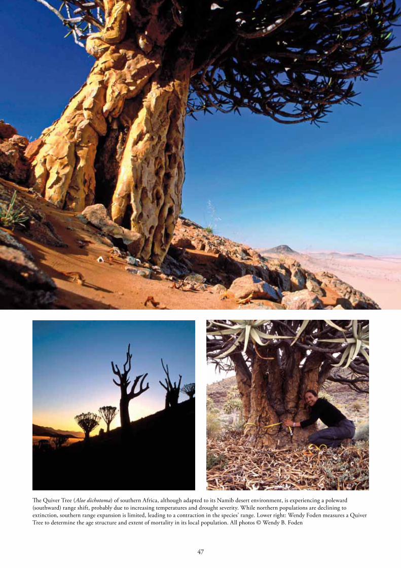
47

The Quiver Tree (Aloe dichotoma) of southern Africa, although adapted to its Namib desert environment, is experiencing a poleward (southward) range shift, probably due to increasing temperatures and drought severity. While northern populations are declining to extinction, southern range expansion is limited, leading to a contraction in the species’ range. Lower right: Wendy Foden measures a Quiver Tree to determine the age structure and extent of mortality in its local population. All photos © Wendy B. Foden

48

IUCN SSC Guidelines for Assessing Species’ Vulnerability to Climate Change

of the earliest applications of correlative models recognized the need to optimize this threshold value (see e.g., Huntley et al., 1995) rather than to use an arbitrary value (e.g., 0.5 as is conventional in logistic regression). The most widely used approach is to select that threshold value that optimizes some measure of goodness-of-fit of the correlative model, the problem being that a large number of such measures have been proposed and used. Liu et al., (2005, 2013) have explored the performance of alternative measures for determining threshold values, both for models fitted to presence–absence data (Liu et al., 2005) and for models fitted to presence-only data (Liu et al., 2013). They conclude in both cases that the threshold value that maximizes the sum of sensitivity and specificity is the only threshold among those they analysed that will have the same value regardless of whether it is calculated using true absences or randomly selected background sites (and also assuming that presences are randomly sampled from the species’ range). This measure is equivalent to one plus the value of the True Skill Statistic (Allouche et al., 2006); maximizing the latter thus gives identical optimal threshold values to maximizing the sum of specificity and sensitivity as proposed by Liu et al. (2005, 2013). Hence, if thresholding is to be performed using a single measure, we recommend that the optimal threshold be selected as that which maximizes the value of the True Skill Statistic. However, as different threshold rules can yield dramatically different conclusions about whether a species will decline or expand under climate change (Nenzén & Araújo, 2011), we recommend carefully experimenting with alternative threshold rules with consideration as to whether optimistic or pessimistic outcomes are more appropriate for the analysis. Furthermore, thresholding will often obscure important differences in environmental suitability between sites – i.e., a site that is moderately suitable and just above the threshold cannot be distinguished from a site that is highly suitable and far above the threshold (Guillera-Arroita et al., 2015). An alternative to thresholding, therefore, is to retain the raw predicted (unthresholded) values of suitability to use in assessing whether environmental conditions improve or degrade for the species (e.g., Still et al., 2015). Furthermore, such assessments of change in overall suitability are a valuable complement to, rather than an alternative to, the use of thresholds to assess potential changes in range extent or degree of range overlap.

5.2.2.2 Inferring population changes from range changesPopulation changes are unlikely to be linearly related to changes in distribution extent because individuals will rarely be evenly spread throughout a species’ overall area of distribution. Nonetheless, in the absence of more specific information, this is an allowable assumption (IUCN SSC Standards and Petitions Subcommittee, 2016), although it should be explicitly stated. Loucks et al., (2010), for example, made such an

assumption when projecting the impacts of future sea-level rise on the population of Panthera tigris (Tiger) in the Sundarbans mangroves. An essential step, however, if such an assumption has to be made, is also to consider firstly whether habitat patches are large enough to support viable subpopulations, given demographic stochasticity and Alee effects, and secondly whether patches projected to be newly available in the future are likely to be colonized by individuals from currently occupied patches (IUCN SSC Standards and Petitions Subcommittee, 2016). Such considerations will be species-specific and thus should be made separately for each taxon for which a CCVA is being performed.

Where species’ abundance, or even data recording an appropriate proxy for abundance, are available, then an alternative approach is to model the relationship between species abundance, as opposed to occurrence, and appropriate bioclimatic variables. Such models can then be used to project the species’ potential future abundance pattern and also to make an assessment of the likely overall change in its population size (see. e.g., Huntley et al., 2012; Renwick et al., 2012; Johnston et al., 2013). The results presented by Huntley et al., (2012) indicated that populations of birds in the area they examined (southern Africa) were projected to decrease by an average of ~50%, whereas range extent was projected to decrease on average by only ~30%. When aggregated, predicted changes in the abundance of seabird and wintering water bird populations on protected areas in response to climate change were significantly correlated with observed national population changes (Johnston et al., 2013), supporting the validity of this approach. Where possible, modelling abundance, rather than occurrence, provides metrics that can be more easily applied to qualifying thresholds for site designation, for red-listing (e.g., Johnston et al., 2013), or to modelling extinction risk. Even where species’ abundance data are not available, most correlative models output a measure of ‘suitability’ or ‘probability of occurrence’ of a species for each grid square. Comparing such values for a projected future climate scenario with those simulated for ‘present’ climate can provide evidence of any likely change in the species’ population over and above that implied by any change in overall range extent. A decrease in mean suitability, for example, would indicate that the species’ population is likely to decrease more than is implied by the decrease in range extent.

Alternative approaches to assessing extinction risks on the basis of correlative model results have also been developed (see e.g., Thomas et al., 2004), but these are not species-specific, giving instead overall estimates of the proportion of species at increased risk of extinction.

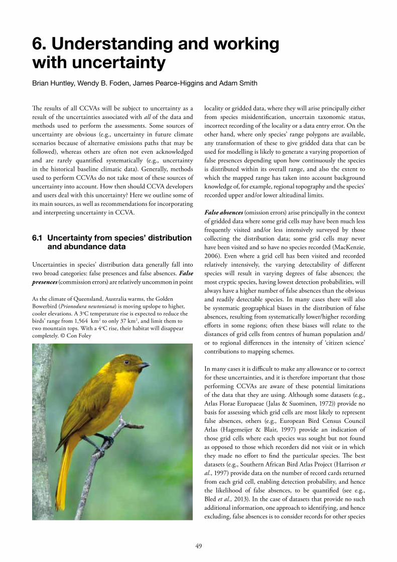
49

The results of all CCVAs will be subject to uncertainty as a result of the uncertainties associated with all of the data and methods used to perform the assessments. Some sources of uncertainty are obvious (e.g., uncertainty in future climate scenarios because of alternative emissions paths that may be followed), whereas others are often not even acknowledged and are rarely quantified systematically (e.g., uncertainty in the historical baseline climatic data). Generally, methods used to perform CCVAs do not take most of these sources of uncertainty into account. How then should CCVA developers and users deal with this uncertainty? Here we outline some of its main sources, as well as recommendations for incorporating and interpreting uncertainty in CCVA.

6.1 Uncertaintyfromspecies’distributionandabundancedata

Uncertainties in species’ distribution data generally fall into two broad categories: false presences and false absences. Falsepresences (commission errors) are relatively uncommon in point

locality or gridded data, where they will arise principally either from species misidentification, uncertain taxonomic status, incorrect recording of the locality or a data entry error. On the other hand, where only species’ range polygons are available, any transformation of these to give gridded data that can be used for modelling is likely to generate a varying proportion of false presences depending upon how continuously the species is distributed within its overall range, and also the extent to which the mapped range has taken into account background knowledge of, for example, regional topography and the species’ recorded upper and/or lower altitudinal limits.

Falseabsences (omission errors) arise principally in the context of gridded data where some grid cells may have been much less frequently visited and/or less intensively surveyed by those collecting the distribution data; some grid cells may never have been visited and so have no species recorded (MacKenzie, 2006). Even where a grid cell has been visited and recorded relatively intensively, the varying detectability of different species will result in varying degrees of false absences; the most cryptic species, having lowest detection probabilities, will always have a higher number of false absences than the obvious and readily detectable species. In many cases there will also be systematic geographical biases in the distribution of false absences, resulting from systematically lower/higher recording efforts in some regions; often these biases will relate to the distances of grid cells from centres of human population and/or to regional differences in the intensity of ‘citizen science’ contributions to mapping schemes.

In many cases it is difficult to make any allowance or to correct for these uncertainties, and it is therefore important that those performing CCVAs are aware of these potential limitations of the data that they are using. Although some datasets (e.g., Atlas Florae Europaeae (Jalas & Suominen, 1972)) provide no basis for assessing which grid cells are most likely to represent false absences, others (e.g., European Bird Census Council Atlas (Hagemeijer & Blair, 1997) provide an indication of those grid cells where each species was sought but not found as opposed to those which recorders did not visit or in which they made no effort to find the particular species. The best datasets (e.g., Southern African Bird Atlas Project (Harrison et al., 1997) provide data on the number of record cards returned from each grid cell, enabling detection probability, and hence the likelihood of false absences, to be quantified (see e.g., Bled et al., 2013). In the case of datasets that provide no such additional information, one approach to identifying, and hence excluding, false absences is to consider records for other species

6.UnderstandingandworkingwithuncertaintyBrian Huntley, Wendy B. Foden, James Pearce-Higgins and Adam Smith

As the climate of Queensland, Australia warms, the Golden Bowerbird (Prionodura newtoniana) is moving upslope to higher, cooler elevations. A 3oC temperature rise is expected to reduce the birds’ range from 1,564  km2 to only 37 km2, and limit them to two mountain tops. With a 4oC rise, their habitat will disappear completely. © Con Foley

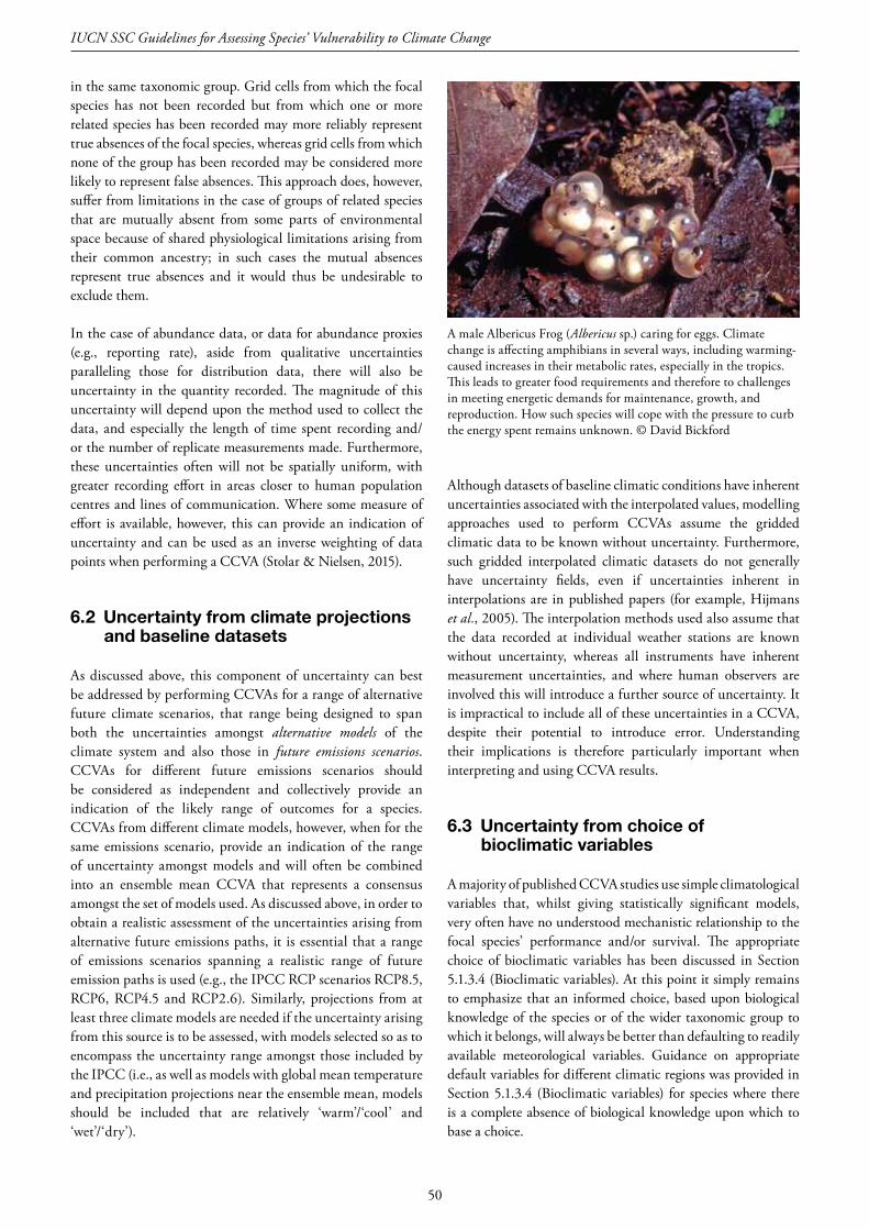
50

IUCN SSC Guidelines for Assessing Species’ Vulnerability to Climate Change

in the same taxonomic group. Grid cells from which the focal species has not been recorded but from which one or more related species has been recorded may more reliably represent true absences of the focal species, whereas grid cells from which none of the group has been recorded may be considered more likely to represent false absences. This approach does, however, suffer from limitations in the case of groups of related species that are mutually absent from some parts of environmental space because of shared physiological limitations arising from their common ancestry; in such cases the mutual absences represent true absences and it would thus be undesirable to exclude them.

In the case of abundance data, or data for abundance proxies (e.g., reporting rate), aside from qualitative uncertainties paralleling those for distribution data, there will also be uncertainty in the quantity recorded. The magnitude of this uncertainty will depend upon the method used to collect the data, and especially the length of time spent recording and/or the number of replicate measurements made. Furthermore, these uncertainties often will not be spatially uniform, with greater recording effort in areas closer to human population centres and lines of communication. Where some measure of effort is available, however, this can provide an indication of uncertainty and can be used as an inverse weighting of data points when performing a CCVA (Stolar & Nielsen, 2015).

6.2 Uncertaintyfromclimateprojectionsandbaselinedatasets

As discussed above, this component of uncertainty can best be addressed by performing CCVAs for a range of alternative future climate scenarios, that range being designed to span both the uncertainties amongst alternative models of the climate system and also those in future emissions scenarios. CCVAs for different future emissions scenarios should be considered as independent and collectively provide an indication of the likely range of outcomes for a species. CCVAs from different climate models, however, when for the same emissions scenario, provide an indication of the range of uncertainty amongst models and will often be combined into an ensemble mean CCVA that represents a consensus amongst the set of models used. As discussed above, in order to obtain a realistic assessment of the uncertainties arising from alternative future emissions paths, it is essential that a range of emissions scenarios spanning a realistic range of future emission paths is used (e.g., the IPCC RCP scenarios RCP8.5, RCP6, RCP4.5 and RCP2.6). Similarly, projections from at least three climate models are needed if the uncertainty arising from this source is to be assessed, with models selected so as to encompass the uncertainty range amongst those included by the IPCC (i.e., as well as models with global mean temperature and precipitation projections near the ensemble mean, models should be included that are relatively ‘warm’/‘cool’ and ‘wet’/‘dry’).

Although datasets of baseline climatic conditions have inherent uncertainties associated with the interpolated values, modelling approaches used to perform CCVAs assume the gridded climatic data to be known without uncertainty. Furthermore, such gridded interpolated climatic datasets do not generally have uncertainty fields, even if uncertainties inherent in interpolations are in published papers (for example, Hijmans et al., 2005). The interpolation methods used also assume that the data recorded at individual weather stations are known without uncertainty, whereas all instruments have inherent measurement uncertainties, and where human observers are involved this will introduce a further source of uncertainty. It is impractical to include all of these uncertainties in a CCVA, despite their potential to introduce error. Understanding their implications is therefore particularly important when interpreting and using CCVA results.

6.3 Uncertaintyfromchoiceofbioclimaticvariables

A majority of published CCVA studies use simple climatological variables that, whilst giving statistically significant models, very often have no understood mechanistic relationship to the focal species’ performance and/or survival. The appropriate choice of bioclimatic variables has been discussed in Section 5.1.3.4 (Bioclimatic variables). At this point it simply remains to emphasize that an informed choice, based upon biological knowledge of the species or of the wider taxonomic group to which it belongs, will always be better than defaulting to readily available meteorological variables. Guidance on appropriate default variables for different climatic regions was provided in Section 5.1.3.4 (Bioclimatic variables) for species where there is a complete absence of biological knowledge upon which to base a choice.

A male Albericus Frog (Albericus sp.) caring for eggs. Climate change is affecting amphibians in several ways, including warming-caused increases in their metabolic rates, especially in the tropics. This leads to greater food requirements and therefore to challenges in meeting energetic demands for maintenance, growth, and reproduction. How such species will cope with the pressure to curb the energy spent remains unknown. © David Bickford

51

Where informed choice nonetheless leaves some degree of uncertainty about the most appropriate bioclimatic variables, then a useful approach is to carry out the modelling required for the CCVA using two or more alternative plausible sets of bioclimatic variables. Measures of the goodness-of-fit and robustness of the alternative models may then indicate that one combination of bioclimatic variables is clearly superior, in which case the CCVA should be based upon those variables. Where alternative combinations of bioclimatic variables give models of similar performance, however, then computing a consensus result amongst the models fitted will be preferable. Such a consensus will best be computed using weighting of the models according to their performance (see e.g., Burnham & Anderson, 2002).

6.4 Uncertaintyfrompotentiallyincompleteevidenceofspecies’niches

A further source of uncertainty relates to the extent to which a species’ realized climatic niche under present climatic conditions fully represents its potentially realizable niche. Where, as is likely to be the case for a majority of species, a species is not currently fully occupying its potentially realizable climatic niche, the results obtained from correlative approaches, on the one hand, and from mechanistic approaches on the other, are both likely to be inaccurate, although for different reasons.

Correlative niche models fitted to species’ present ranges generally are likely substantially to under-estimate the potentially realizable niche, and hence overestimate vulnerability (Varela et al., 2009), because species are likely in future potentially to be able to extend their ranges into areas offering combinations of climatic conditions that don’t currently occur, but that become available as a result of future climate changes (Williams et al., 2007). Evidence of the importance of this issue comes from the Pleistocene fossil record that includes frequent occurrences of no-analogue combinations of species associated with past climatic conditions for which no current analogue exists (Huntley, 1990; Overpeck et al., 1992; Graham et al., 1996; Williams et al., 2001; Jackson & Williams, 2004).

In contrast, the mechanistic approach, which uses experimental and other direct evidence of species’ climatic tolerances, provides an estimate of the species’ fundamental climatic niche that will almost certainly be an overestimate of its potentially realizable niche, because interactions with other species play a large role in determining the areas of climatic space a species can occupy. Mechanistic approaches are thus likely to underestimate vulnerability to climate change. The same is true of niche modelling approaches that are based upon identifying, from species’ present distributions, bioclimatic limits to their occurrence, and then applying these independently to generate hyper-rectangular climatic niches (e.g., minimal rectilinear envelope modelling as applied by Svenning & Skov, 2004).

Such approaches ignore a wealth of evidence that indicates that bioclimatic variables commonly have interacting effects when determining species’ ranges (Huntley, 2001), as well as the large volume of evidence of indirect effects of biotic interactions in limiting species’ realized climatic niches (e.g., Woodward, 1975). As a result, these methods generate gross over-estimates of species’ potentially realizable niches, and if used in a CCVA would be likely very seriously to underestimate vulnerability to climate change.

One of the few sources of information that can be used to learn about a species’ potentially realizable climatic niche is the Pleistocene fossil record, but unfortunately this is available for only a minority of species, mostly mammals (e.g., Ovibos moschatus MacPhee et al. (2005); Saiga tatarica Campos et al. (2010) and higher plants, especially wind-pollinated temperate trees that are regionally monotypic (e.g., Fagus sylvatica and F. grandifolia in Europe and North America respectively), and even then is far from complete.

6.5 Uncertaintyfrombiologicaltraitanddemographicdata

It is worth recognizing that a number of key uncertainties are associated with TVAs. Firstly, although increasingly studied, the importance of species-traits in influencing species’ vulnerability to climate change is relatively undescribed and uncertain, with different studies showing variation in importance (e.g., Dobrowski et al., 2011; Angert et al., 2011; Pearson et al., 2014b). Although an increasing evidence base is building around the importance of particular traits affecting species’ vulnerability to climate change (e.g., Pearce-Higgins et al., (2015) for birds; Pearson et al., (2014a) for amphibians), we do not yet know which are the most important, and how that importance may vary among species and locations (Pacifici et al., 2015; Willis et al., 2015) (see also sections 5.1.5.4 Calculating overall measures of vulnerability and 5.1.5.5 Missing data, uncertainty, variability, and inapplicability in this report.) Challenges to the development of a cohesive evidence base include accounting for the many traits and variables that may drive vulnerability, the interactions between these traits and the lack of standardization between the published studies on which such an evidence base would rely (Estrada et al., 2016).

Secondly, and related to this, there is little consensus about how information about different traits should be scored or combined to assess vulnerability, making it difficult to compare the results of different approaches (Willis et al., 2015), and resulting in there being no overall assessment of the actual magnitude of projected risk across species. Thirdly, the ability of experts to assess ecological traits also remains uncertain. Given that expert judgement can be subject to bias (Burgman et al., 2011), it is important to ensure that where it is used, a clear and valid methodology is applied to such expert-based assessment.

6. Understanding and working with uncertainty

52

IUCN SSC Guidelines for Assessing Species’ Vulnerability to Climate Change

Given the inevitable gaps in availability of biological and trait-based data, those performing CCVAs using trait-based or mechanistic methods will often have to resort to using best estimates for the values of missing data, for example by using values for close relatives where these are known. The use of such best estimates, however, inevitably introduces an additional degree of uncertainty. Even where data are available, they are subject to numerous other sources of uncertainty. Most biological and demographic characteristics, for example, show varying degrees of intraspecific, spatial and temporal variability. Such uncertainties in best estimates and variability in measurements should be taken into account when performing mechanistic or trait-based CCVAs, ideally by performing an ensemble of analyses using a range of plausible estimates for each value in order to assess the overall uncertainty in the CCVA result.

In many cases, the only available data have been gathered from laboratory experiments (e.g., physiological tolerances) or from ex situ individuals such as those in zoos, botanical gardens or breeding programmes (e.g., longevity, age at first reproduction, litter size); the inherent biases in data from such sources should be considered if they must be used. On the other hand, field-based measurements of tolerances may confound the effects of phenotypic plasticity, epigenetic mechanisms and genetics, and thus also provide biased estimates.

It is important to distinguish uncertainty (lack of knowledge) from variability (natural variation in traits with species; cf. (Lehmann & Rillig, 2014b). The former can be rectified by gap-filling as mentioned above or otherwise accounted for in a scoring system (5.1.5.5 Missing data, uncertainty, variability, and inapplicability). In contrast, intraspecific variation in traits cannot be absolved through more research or gap-filling – it reflects actual differences between individuals and populations within a species. Methods for reflecting intraspecific variation in traits in CCVA are discussed in Section 5.1.6.5 Missing data, uncertainty, variability, and inapplicability.

6.5.1Changesintraitsovertime

Traits used for predicting climate change vulnerability (e.g., body size, fecundity and energy requirements) may themselves be subject to selection by climatic conditions and thus may change as climate changes (Isaac, 2009). For example, warming and decreases in dissolved oxygen are predicted to lead to decreased body sizes in marine fishes (Cheung et al., 2012). According to Bergmann’s Rule, which proposes a global pattern of decreasing body size along a gradient from cooler to warmer regions due to the advantages of a lower surface area to volume ratio in cooler climates (Freckleton et al., 2003; Clauss et al., 2013), a trend of decreasing body size might be expected as climate warms. Some experimental and observational studies have found evidence for this (Sheridan & Bickford, 2011), but there are also contradictory data (Teplitsky & Millien,

2013). Species’ capacities for such an adaptive response may be provided by one or both of phenotypic plasticity or genetic evolution across generations, and individual species’ capacities for such adaptive responses may be important determinants of their degree of climate change vulnerability. Phenological changes (i.e., changes in the timing of events such as flowering and reproduction), the underlying mechanism for which may again be either phenotypic plasticity or genetic evolution, seem to be a particularly important adaptive response in both plants and animals, although species and even major taxonomic groups show different rates and magnitudes of responses to the climate changes of the past century (Root et al., 2003). Such often under-appreciated vulnerability traits, although challenging to quantify, can and should be incorporated when applying mechanistic and trait-based approaches (Chown et al., 2010).

6.6Uncertaintyfromchoiceofmethod

6.6.1Correlativeapproaches

Uncertainties arising from the choice of modelling technique have received considerable attention in the literature, and there has been widespread advocacy of an ensemble approach that utilizes a range of alternative methods and takes a mean (often weighted) of the results obtained from these methods (Thuiller, 2003; Araújo & New, 2007; Marmion et al., 2009). Unfortunately, the issue of selecting appropriate and rejecting inappropriate methods to include in such ensembles has received much less attention. An appropriate choice is essential, however, because at least some methods used in published studies make inappropriate assumptions, firstly about the form of the relationships being modelled and secondly about the nature of the interactive effects of two or more bioclimatic variables on species. Including methods that make such inappropriate assumptions in an ensemble is likely to result in a less reliable consensus result, and certainly one that is less robust, than would be obtained from a more limited ensemble of models, or perhaps even just a single model, that do/does not make such assumptions.

Many methods assume some particular form of the relationship between a species’ probability of occurrence and each bioclimatic variable, some for example assuming a linear relationship and others a symmetrical Gaussian or ‘bell-shaped’ relationship, whereas in reality the realized relationships usually are more complex (Austin, 2007). Similarly, some methods assume no interactions between the bioclimatic variables determining a species’ range (e.g., minimal rectilinear envelope modelling as applied by Svenning & Skov (2004); once again ample evidence indicates that this is not a valid assumption. The most appropriate methods arguably are thus those that make no prior assumption about the form of the relationships being modelled and that allow for interacting effects of the bioclimatic variables. Ideally models should be fitted across the range of

53

the species, allowing for non-stationary interactions between bioclimatic variables and for complex forms of the relationships of species’ probability of occurrence and bioclimatic variables. A non-exhaustive list of preferred methods would include: generalized additive models (GAMs) with appropriate choice of smoother (e.g., smoothing splines) (Yee & Mitchell, 1991); climatic response surfaces fitted by locally-weighted regression (Huntley et al., 1995); and classification and regression trees (De’ath & Fabricius, 2000).

In the context of CCVA, a major source of uncertainty relates to the fact that most modelling techniques behave unpredictably when, as will almost inevitably be the case, predictions of species’ potential future ranges require extrapolations into areas of climatic space (i.e., combinations of bioclimatic variable values) that are projected to be available in the future but that are not currently found anywhere within the domain of the data used to fit the model. For this reason wise precautions include mapping areas that are projected to have future climates without current analogues, using appropriate tools to characterize such novelty in future climates, and/or using methods that enable predictions made by extrapolation to be identified (Platts et al., 2008; Fitzpatrick & Hargrove, 2009; Elith et al., 2010; Zurell et al., 2012). Combining such precautions with the use of methods that behave in a conservative and predictable manner when extrapolated (e.g., climatic response surfaces fitted by locally-weighted regression that make predictions beyond the scope of the fitting domain that are asymptotic

to the values at the margins of that domain, (Huntley et al., 2007)) avoids the pitfalls associated with methods that are prone to give unrealistic predictions outside the fitting domain (e.g., generalized linear models using polynomial relationships may give response curves for individual variables that predict increase, decrease or no change in environmental suitability in regions beyond the range of the training data, any or all of which may be realistic or completely unrealistic).

Another important source of uncertainty is bias in the presence records or presence cells used to train the correlative model. At global scales collection effort is concentrated around areas of high endemism, close to research institutions, and in wealthier countries (Meyer et al., 2015), while at finer scales collection effort is often concentrated along areas of access (roads, rivers) and close to major population centres (Phillips et al., 2009). As discussed in Section 5.1.4 Species distribution data, methods exist to remove these biases. Nonetheless, differentiating sampling bias from genuine differences in density of the species across its range can be difficult and thus introduce uncertainty.

An additional source of uncertainty arises in the case of methods that use presence-only data, as opposed to presence–absence data, because most of these methods do not use only the presences but must also use pseudo-absences or background sites in order to fit a model (Elith et al., 2006), and all require pseudo-absences or background sites in order to evaluate conventional measures of model goodness-of-fit that are based upon the four values in the confusion matrix (Figure 10). Pseudo-absences are sites selected in a manner that attempts to ensure that the species is absent from a location (even though there may have been no search effort in that location for the species). Pseudo-absences are used to stand in for “true” absences. In contrast, background sites can be located across a landscape regardless of whether a species is present or absent from a particular site. Some algorithms can use either pseudo-absences or background sites (e.g., generalized additive models and linear models), while other methods should only be used with background sites (e.g., Maxent; Merow et al., 2013). How these pseudo-absences or background sites are selected varies, with different selection methods resulting in models that differ in performance and in the robustness of their predictions (Phillips et al., 2009). In many cases the overall extent of the climatic space defined for fitting determines the space within which pseudo-absences or background sites are selected, but the larger the climatic space that is defined, the less well the species’ ‘true’ climatic envelope is constrained, often resulting

Narwhals (Monodon monoceros) have been ranked by an expert panel as one of the most climate change sensitive species in the Arctic because of their limited distribution, specialized diet and high dependence on sea ice environments. © Magnus Andersen, NPI

Model predictionsObservations

Presence Absence

Presence a b

Absence c d

Figure 10. Confusion matrix.

6. Understanding and working with uncertainty

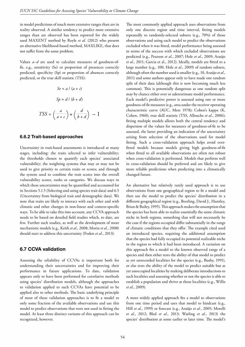
54

IUCN SSC Guidelines for Assessing Species’ Vulnerability to Climate Change

in model predictions of much more extensive ranges than are in reality observed. A similar tendency to predict more extensive ranges than are observed has been reported for the widely used MAXENT method by Royle et al. (2012) who present an alternative likelihood-based method, MAXLIKE, that does not suffer from the same problem.

Values a–d are used to calculate measures of goodness-of-fit, e.g., sensitivity (Se) or proportion of presences correctly predicted, specificity (Sp) or proportion of absences correctly predicted, or the true skill statistic (TSS):

Se = a / (a + c)

Sp = d / (b + d)

6.6.2Trait-basedapproaches

Uncertainty in trait-based assessments is introduced at many stages, including: the traits selected to infer vulnerability; the thresholds chosen to quantify each species’ associated vulnerability; the weighting systems that may or may not be used to give priority to certain traits or scores; and through the system used to combine the trait scores into the overall vulnerability scores, ranks or categories. We discuss ways in which these uncertainties may be quantified and accounted for in Sections 5.1.5 (Selecting and using species trait data) and 6.5 (Uncertainty from biological trait and demographic data). We note that traits are likely to interact with each other and with climatic and other changes in non-linear and context-specific ways. To be able to take this into account, any CCVA approach needs to be based on detailed field studies which, to date, are few. Further such studies, as well as the development of more mechanistic models (e.g., Keith et al., 2008; Morin et al., 2008) should start to address this uncertainty (Foden et al., 2013).

6.7CCVAvalidation

Assessing the reliability of CCVAs is important both for understanding their uncertainties and for improving their performance in future applications. To date, validation appears only to have been performed for correlative methods using species’ distribution models, although the approaches to validation applied to such CCVAs have potential to be applied also to other methods. The basic underlying principle of most of these validation approaches is to fit a model to only some fraction of the available observations and use this model to predict observations that were not used in fitting the model. At least three distinct variants of this approach can be recognized, however.

The most commonly applied approach uses observations from only one discrete region and time interval, fitting models repeatedly to randomly-selected subsets (e.g., 70%) of those observations and using each model to predict the observations excluded when it was fitted, model performance being assessed in terms of the success with which excluded observations are predicted (e.g., Pearson et al., 2007; Hole et al., 2009; Araújo et al., 2011; Garcia et al., 2012). Ideally, models are fitted to a large number (e.g., 100, Hole et al., 2009) of random subsets, although often the number used is smaller (e.g., 10, Araújo et al., 2011) and some authors appear only to have made one random split of their data (although this is now becoming much less common). This is potentially dangerous as one random split may by chance either over or uderestimate model performance. Each model’s predictive power is assessed using one or more goodness-of-fit measures (e.g., area under the receiver operating characteristic curve (AUC, Metz 1978); Cohen’s kappa (K, Cohen, 1960); true skill statistic (TSS, Allouche et al., 2006); fitting multiple models allows both the central tendency and dispersion of the values for measures of goodness-of-fit to be assessed, the latter providing an indication of the uncertainty arising from selection of the observations used for model fitting. Such a cross-validation approach helps avoid over-fitted models because models giving high goodness-of-fit when fitted to all available observations are often not robust when cross-validation is performed. Models that perform well in cross-validation should be preferred and are likely to give more reliable predictions when predicting into a climatically changed future.

An alternative but relatively rarely used approach is to use observations from one geographical region to fit a model and then use the model to predict the species’ distribution in a different geographical region (e.g., Beerling, David J., Huntley, Brian & Bailey, 1995). This approach makes the assumption that the species has been able to realize essentially the same climatic niche in both regions, something that will not necessarily be the case if the regions occupied differ substantially in the range of climatic conditions that they offer. The example cited used an introduced species, requiring the additional assumption that the species had fully occupied its potential realizable niche in the region to which it had been introduced. A variation on this approach fits a model to the known observed range of a species and then either tests the ability of that model to predict as yet unrecorded localities for the species (e.g., Busby, 1991), or else tests the ability of the model to predict suitable but as yet unoccupied localities by making deliberate introductions to such localities and assessing whether or not the species is able to establish a population and thrive at those localities (e.g., Willis et al., 2009).

A more widely applied approach fits a model to observations from one time period and uses that model to hindcast (e.g., Hill et al., 1999) or forecast (e.g., Araújo et al., 2005; Morelli et al., 2012; Bled et al., 2013; Watling et al., 2013) the species’ distribution at some earlier or later time. The model’s

TSS =a

a + c + – 1( ) db + d( )

55

predictions for the period from which data were not used in fitting the model are then assessed using observations from that time, either qualitatively in terms of broad visual comparison, where systematic comparison is not possible or inappropriate, or as before using appropriate measures of goodness-of-fit. In principle, this approach can be extended to use models fitted to species’ present distributions to make hindcasts of their potential distributions for periods in the late Quaternary that are then compared with the available fossil record for the species; however, the general scarcity of fossil remains identifiable to the species level severely limits the application of such an approach. Nonetheless, such hindcasts can provide valuable insights into species’ potential past ranges that can aid our understanding of present distributions and behaviour (e.g., Ruegg et al., 2006; Huntley et al., 2014).

An alternative validation approach involves fitting a model to presence–absence observations from one time period and using it to forecast/hindcast changes not in species’ presence or absence, but in the raw climatic suitability values output by the model. The predicted changes in climatic suitability can

then be compared with observed changes in population size of the species (e.g., Green et al., 2008; Gregory et al., 2009). Such an approach provides robust and convincing validation of the correlative modelling approach, but is only possible in areas

Lasius balearicus. © Gerard Talavera

Only described as a new species in 2014, Lasius balearicus, is an ant species restricted to the highest summits (800 m to 1,400 m above sea level) of the Serra de Tramuntana mountains of Majorca, Spain. The species is considered to be in danger of extinction due both to its extremely small range and because correlative models predict climate change driven declines in range suitability such that it may soon become extinct. © Roger Vila

56

IUCN SSC Guidelines for Assessing Species’ Vulnerability to Climate Change

and for species with good, typically long-term, monitoring datasets (e.g., rare birds breeding in the UK, Green et al., 2008; European breeding birds, Gregory et al., 2009). A related approach compares raw predicted values to measures like body size, fecundity, or other metrics of population-level fitness (e.g., Wittmann et al., 2016).

Evidence of the general robustness of the expectation that species’ geographical ranges track changes in climate (Huntley & Webb, 1989) can be provided by studies showing such responses over the past century (e.g., Tingley et al., 2009; Chen

et al., 2011). Such evidence provides further corroborative support for the validity of the general approach used by CCVA methods based upon species’ distribution models, even if no formal validation of a model is performed in the sense described above. Use of such observation-based validation is an important priority for those developing and using trait-based approaches; the observational data needs, however, limit the use of recently observed changes for such CCVA validation to areas and species with high quality long-term observation records.

The Joshua Tree (Yucca brevifolia) is threatened by increased temperatures and decreased rainfall in its desert habitat in the southwest of North America. The range of this unusual tree is predicted to contract poleward (northward) and split into isolated populations. While some simulations project expansion into new habitat, observed dispersal rates (both current and historical) seem to indicate the trees will be unable to do so. © kevinschafer.com

56

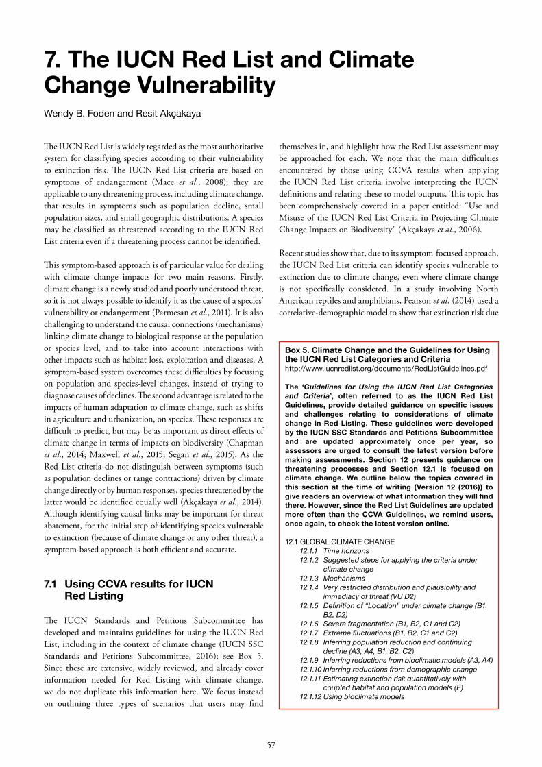
57

The IUCN Red List is widely regarded as the most authoritative system for classifying species according to their vulnerability to extinction risk. The IUCN Red List criteria are based on symptoms of endangerment (Mace et al., 2008); they are applicable to any threatening process, including climate change, that results in symptoms such as population decline, small population sizes, and small geographic distributions. A species may be classified as threatened according to the IUCN Red List criteria even if a threatening process cannot be identified.

This symptom-based approach is of particular value for dealing with climate change impacts for two main reasons. Firstly, climate change is a newly studied and poorly understood threat, so it is not always possible to identify it as the cause of a species’ vulnerability or endangerment (Parmesan et al., 2011). It is also challenging to understand the causal connections (mechanisms) linking climate change to biological response at the population or species level, and to take into account interactions with other impacts such as habitat loss, exploitation and diseases. A symptom-based system overcomes these difficulties by focusing on population and species-level changes, instead of trying to diagnose causes of declines. The second advantage is related to the impacts of human adaptation to climate change, such as shifts in agriculture and urbanization, on species. These responses are difficult to predict, but may be as important as direct effects of climate change in terms of impacts on biodiversity (Chapman et al., 2014; Maxwell et al., 2015; Segan et al., 2015). As the Red List criteria do not distinguish between symptoms (such as population declines or range contractions) driven by climate change directly or by human responses, species threatened by the latter would be identified equally well (Akçakaya et al., 2014). Although identifying causal links may be important for threat abatement, for the initial step of identifying species vulnerable to extinction (because of climate change or any other threat), a symptom-based approach is both efficient and accurate.

7.1 UsingCCVAresultsforIUCN RedListing

The IUCN Standards and Petitions Subcommittee has developed and maintains guidelines for using the IUCN Red List, including in the context of climate change (IUCN SSC Standards and Petitions Subcommittee, 2016); see Box 5. Since these are extensive, widely reviewed, and already cover information needed for Red Listing with climate change, we do not duplicate this information here. We focus instead on outlining three types of scenarios that users may find

themselves in, and highlight how the Red List assessment may be approached for each. We note that the main difficulties encountered by those using CCVA results when applying the IUCN Red List criteria involve interpreting the IUCN definitions and relating these to model outputs. This topic has been comprehensively covered in a paper entitled: “Use and Misuse of the IUCN Red List Criteria in Projecting Climate Change Impacts on Biodiversity” (Akçakaya et al., 2006).

Recent studies show that, due to its symptom-focused approach, the IUCN Red List criteria can identify species vulnerable to extinction due to climate change, even where climate change is not specifically considered. In a study involving North American reptiles and amphibians, Pearson et al. (2014) used a correlative-demographic model to show that extinction risk due

7.TheIUCNRedListandClimateChangeVulnerabilityWendy B. Foden and Resit Akçakaya

Box5.ClimateChangeandtheGuidelinesforUsingtheIUCNRedListCategoriesandCriteriahttp://www.iucnredlist.org/documents/RedListGuidelines.pdf

The ‘Guidelines for Using the IUCN Red List Categories and Criteria’, often referred to as the IUCN Red ListGuidelines,providedetailedguidanceonspecific issuesand challenges relating to considerations of climatechange inRedListing.TheseguidelinesweredevelopedbytheIUCNSSCStandardsandPetitionsSubcommitteeand are updated approximately once per year, soassessorsareurged toconsult the latestversionbeforemaking assessments. Section 12 presents guidance onthreatening processes and Section 12.1 is focused onclimate change. We outline below the topics covered inthis section at the time of writing (Version 12 (2016)) togivereadersanoverviewofwhatinformationtheywillfindthere.However,sincetheRedListGuidelinesareupdatedmore often than the CCVA Guidelines, we remind users,onceagain,tocheckthelatestversiononline.

12.1 GLOBAL CLIMATE CHANGE12.1.1 Time horizons12.1.2 Suggested steps for applying the criteria under

climate change12.1.3 Mechanisms12.1.4 Very restricted distribution and plausibility and

immediacy of threat (VU D2)12.1.5 Definition of “Location” under climate change (B1,

B2, D2)12.1.6 Severe fragmentation (B1, B2, C1 and C2)12.1.7 Extreme fluctuations (B1, B2, C1 and C2) 12.1.8 Inferring population reduction and continuing

decline (A3, A4, B1, B2, C2) 12.1.9 Inferring reductions from bioclimatic models (A3, A4) 12.1.10 Inferring reductions from demographic change12.1.11 Estimating extinction risk quantitatively with

coupled habitat and population models (E)12.1.12 Using bioclimate models

58

IUCN SSC Guidelines for Assessing Species’ Vulnerability to Climate Change

to climate change can be predicted by information available in the present day, such as current occupied area and population size, much of which is used in the IUCN Red List criteria. Using the same species and climate projections, Stanton et al. (2015) showed that IUCN Red List criteria can identify species that would go extinct because of climate change without conservation action, and can do so with decades of warning time. Warning time is defined as the time between when a species is first identified as threatened and when it goes extinct (assuming no conservation action), and is the time available for the cause of the decline to be identified and for conservation measures to be implemented to address the threat and prevent the extinction of a species.

There has been concern that the Red List criteria may not be adequate for assessing species threatened with climate change, particularly because many species that are projected to undergo substantial range contractions in the next several decades have generation lengths that are too short to trigger the relevant IUCN Red List criteria, which consider declines over a three-generation period (Akçakaya et al., 2006). Keith et al. (2014), however, found that warning times were sufficient for a short-lived Australian amphibian, and Stanton et al. (2015) showed that shorter generation lengths did not decrease the power of the Red List to predict climate change-driven extinction risk.

Three important factors contribute to the Red List’s ability to predict climate change-driven extinction risk. The first is the quality and amount of information used for Red Listing; lack of information often results in only one criterion being used for assessing a species’ status, which is problematic since both Keith et al. (2014) and Stanton et al. (2015) show that using a single criterion results in shorter warning times. Stanton et al. (2015) show that although average warning time is over 60 years when all criteria are used, it is as short as 20 years when only a single criterion is used. Secondly, regular monitoring of

species is required if symptoms of changes in population and range sizes are to be detected and used (Keith et al., 2014). The nature or threat and the concept of ‘warning times’ means that it is also critical to regularly reassess species already listed on the Red List. This is particularly important in data-poor situations. Akçakaya et al. (2014) and Stanton et al. (2015) show, for example, that when data constraints allow use of only one criterion, annual or 5-year, instead of 10-year reassessment intervals, increase warning times substantially. Finally, warning time is likely to be too short if conservation action is started only when a species is listed at the highest IUCN threat category (Critically Endangered).

7.2 ThreeuserscenariosforRedListing

consideringClimateChange

We begin with the simplest scenario, which is oriented for a resource-poor context, and continue to those scenarios where greater resources are available.

Scenario 1: Consider the species’ ecological and biological traits to determine the likely mechanisms of climate change impact and quantify these using expert knowledge

Climate change can affect populations via many mechanisms; and thinking about how this will occur for given taxa can clarify the parameters and criteria relevant for a Red List assessment. In this scenario, an assessor may not have the data or expertise to model climate change impacts, but does have information on the physiology, behaviour and ecology of the focal species. Assessors should consider this information to determine the likely mechanisms of both direct and indirect climate change impacts, those from climate change interactions with other threats (e.g., invasive species, habitat loss) and the impacts of human responses to climate change.

A Coral Crisis working group meeting was held at the Royal Society, London in July 2009. Co-chaired by Sir David Attenborough, coral reef and climate change specialists outlined seven key points about the vulnerability of coral reefs to climate change globally. These were then communicated to the public and press through an emergency position statement, delivered by Sir David, and through a supporting publication. Left: Staghorn corals © Lyndon Devantier. Right: Coral Crisis working group meeting © Sonia Khela

59

To apply the Red List criteria, assessors are required to quantify the impacts of these mechanisms on the species to determine whether they meet the thresholds for the Red List threat categories. To do this, we recommend that assessors rank the listed mechanisms according to the degree and likelihood of impact, and for the dominant mechanisms or threats, estimate their plausibility (how likely they are to impact), immediacy (how soon they are expected to impact), geographic scope (where they are likely to impact) and severity (how much they are likely to impact the species’ population or distribution range). The Red List Guidelines provide detailed guidance on how to carry this out, and how Red List concepts such as “location,” “severely fragmented,” “extreme fluctuations,” “population reductions,” “very restricted distribution” and “continuing decline” should be interpreted in this context. The justification of these estimates or projections should be specified in threats and assessment rationales. Since some of this information may be based on expert knowledge, as many experts as possible should be involved and consensus reached wherever possible. Note that many of the variables used in this process (such as location, severe fragmentation, restricted distribution) require spatial information, and the calculation of the others (in particular, reduction and estimated continuing decline) must consider the variability of rates of change across the species’ range. Therefore, detailed maps of the species’ range and other types of spatially explicit data need to be considered in this scenario.

Scenario 2: Use correlative model outputs to quantify climate change impacts on species’ distribution ranges

Where correlative model results are available, or where assessors are able to carry these out, they can provide a valuable way to project and quantify the direct impacts of bioclimatic changes on species’ distribution ranges. This is particularly valuable for projecting declines in distribution ranges, and can be used to infer changes in population sizes. The IUCN Red List Guidelines (Section 12.1.12 Using bioclimatic models) give specific guidance on how these two components should be derived and interpreted from the models, as well as their use in assigning species into threat categories. Section 4.1 of the Red List guidelines provides steps for assessing the robustness of the data and methods used in existing model outputs, and Sections 5 and 6 provide guidance for those wishing to build their own bioclimatic models. An important consideration is that the

selection of predictor variables to include in these models needs to be informed by the likely mechanisms of climate change impact, as outlined in scenario 1.

It is important to recognize that correlative models typically focus only on direct climatic impacts from climate change, and impacts from aspects such as changes in species interactions, disruptions to cues, climate change interaction with other threats and human responses to climate change, are not considered. The CCVA Guidelines discuss ways in which bioclimatic models can and have been combined with trait-based and demographic models to consider other possible mechanisms of impacts; understanding of likely changes in interactions with other species can also be improved by carrying out bioclimatic modelling on key interacting species (e.g., prey or pollinators). To thoroughly explore the full range of potential climate change impacts, however, we recommend that assessors also carry out a full inventory of likely climate change impact mechanisms on the focal species (see Scenario 1), and use the Red List Guidelines to interpret how these can be quantified to contribute to the Red List assessment. Scenario 3: Use mechanistic model outputs to quantify climate change impacts on populations and ranges

Where mechanistic model results are available, or where assessors are able to build such models, they can provide a valuable way to project and quantify both direct and indirect impacts of climate change on a range of possible species parameters including population sizes, distribution ranges, interspecies interactions and overall species extinction risk. Because mechanistic models typically require significant data and expertise, they are generally constructed for fewer species.

In most cases, their spatial component will be based on results of the correlative models, so this step is dependent on the previous one, and the relevant Red List and CCVA Guidelines sections should be consulted. In addition, the demographic model components will also need to be reviewed. Few models are likely to be able to include all of the direct, indirect and interacting effects of climate change on the focal species, so we also recommend that assessors carry out an impact mechanism inventory (described in Scenario 1) in order to identify any additional potentially important climate-driven threats to the species.

7. The IUCN Red List and Climate Change Vulnerability

60

IUCN SSC Guidelines for Assessing Species’ Vulnerability to Climate Change

Temperature increases and changing rainfall seasonality are expected to increase fire frequency and intensity in South Africa’s Cape Floral Kingdom, affecting species such as the King Protea (Protea cynaroides). © Wendy B. Foden

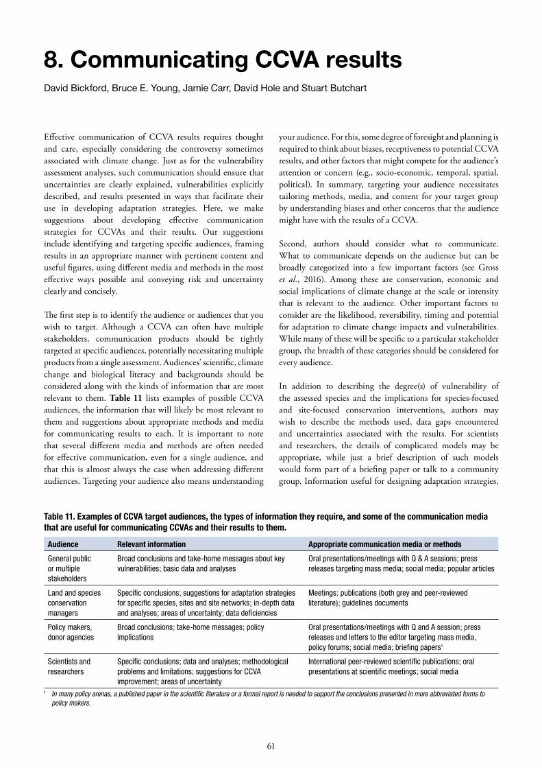
61

Effective communication of CCVA results requires thought and care, especially considering the controversy sometimes associated with climate change. Just as for the vulnerability assessment analyses, such communication should ensure that uncertainties are clearly explained, vulnerabilities explicitly described, and results presented in ways that facilitate their use in developing adaptation strategies. Here, we make suggestions about developing effective communication strategies for CCVAs and their results. Our suggestions include identifying and targeting specific audiences, framing results in an appropriate manner with pertinent content and useful figures, using different media and methods in the most effective ways possible and conveying risk and uncertainty clearly and concisely.

The first step is to identify the audience or audiences that you wish to target. Although a CCVA can often have multiple stakeholders, communication products should be tightly targeted at specific audiences, potentially necessitating multiple products from a single assessment. Audiences’ scientific, climate change and biological literacy and backgrounds should be considered along with the kinds of information that are most relevant to them. Table 11 lists examples of possible CCVA audiences, the information that will likely be most relevant to them and suggestions about appropriate methods and media for communicating results to each. It is important to note that several different media and methods are often needed for effective communication, even for a single audience, and that this is almost always the case when addressing different audiences. Targeting your audience also means understanding

your audience. For this, some degree of foresight and planning is required to think about biases, receptiveness to potential CCVA results, and other factors that might compete for the audience’s attention or concern (e.g., socio-economic, temporal, spatial, political). In summary, targeting your audience necessitates tailoring methods, media, and content for your target group by understanding biases and other concerns that the audience might have with the results of a CCVA.

Second, authors should consider what to communicate. What to communicate depends on the audience but can be broadly categorized into a few important factors (see Gross et al., 2016). Among these are conservation, economic and social implications of climate change at the scale or intensity that is relevant to the audience. Other important factors to consider are the likelihood, reversibility, timing and potential for adaptation to climate change impacts and vulnerabilities. While many of these will be specific to a particular stakeholder group, the breadth of these categories should be considered for every audience.

In addition to describing the degree(s) of vulnerability of the assessed species and the implications for species-focused and site-focused conservation interventions, authors may wish to describe the methods used, data gaps encountered and uncertainties associated with the results. For scientists and researchers, the details of complicated models may be appropriate, while just a brief description of such models would form part of a briefing paper or talk to a community group. Information useful for designing adaptation strategies,

8.CommunicatingCCVAresultsDavid Bickford, Bruce E. Young, Jamie Carr, David Hole and Stuart Butchart

Table 11. Examples of CCVA target audiences, the types of information they require, and some of the communication media that are useful for communicating CCVAs and their results to them.

Audience Relevant information Appropriate communication media or methods

Generalpublicormultiplestakeholders

Broadconclusionsandtake-homemessagesaboutkeyvulnerabilities;basicdataandanalyses

Oralpresentations/meetingswithQ&Asessions;pressreleasestargetingmassmedia;socialmedia;populararticles

Landandspeciesconservationmanagers

Specificconclusions;suggestionsforadaptationstrategiesforspecificspecies,sitesandsitenetworks;in-depthdataandanalyses;areasofuncertainty;datadeficiencies

Meetings;publications(bothgreyandpeer-reviewedliterature);guidelinesdocuments

Policymakers,donoragencies

Broadconclusions;take-homemessages;policyimplications

Oralpresentations/meetingswithQandAsession;pressreleasesandletterstotheeditortargetingmassmedia,policyforums;socialmedia;briefingpapers1

Scientistsandresearchers

Specificconclusions;dataandanalyses;methodologicalproblemsandlimitations;suggestionsforCCVAimprovement;areasofuncertainty

Internationalpeer-reviewedscientificpublications;oralpresentationsatscientificmeetings;socialmedia

1 In many policy arenas, a published paper in the scientific literature or a formal report is needed to support the conclusions presented in more abbreviated forms to policy makers.

62

IUCN SSC Guidelines for Assessing Species’ Vulnerability to Climate Change

such as species’ physiological tolerances, life histories and/or landscape contexts, is key to informing the development and implementation of these conservation actions. For conservation practitioners, spatially explicit results are also likely to be valuable for developing adaptation strategies, and maps depicting these results should include a spatial context (political boundaries, roads, park boundaries and populated areas) that the audience can relate to.

A third suggestion is that authors need to think about how to communicate, and to make effective use of available media and visual aids (e.g., graphs, tables, maps and figures) for dissemination. Use of colour in graphics to indicate relative vulnerability of the species assessed and error bars to indicate the limits of uncertainty can be powerful means of communication (e.g., Dubois et al., 2011). Increasingly, project leaders are using short videos to describe their findings to general audiences. Emotional segments of wildlife and testimonials from rural farmers affected by climate change are techniques used to help these videos connect with broad audiences. Media such as brief reports, graphs and summary tables can quickly convey complexities that are hard to explain in other ways. When writing, authors also should pay attention to clear articulation of terms and avoidance of undefined acronyms or obscure technical jargon. A medium that is becoming increasingly useful for disseminating results to broad audiences is social media. For example, Twitter, Facebook, and Instagram posts that include striking images, graphs and videos can direct audiences toward more in-depth reports, briefing notes and media reports about vulnerability assessment results, while enabling the popularization of ideas that might otherwise be overlooked in decision-making processes.

Finally, it is important to be aware of the problems inherent in communicating CCVA results. Two particular kinds of content that need special attention are those of uncertainty and vulnerability. Scientific uncertainty is vastly different to the common use of the term, and this point needs to be clearly refreshed for certain audiences. While uncertainty needs to be made transparent, authors are strongly urged to clarify that uncertainty does not mean ignorance. Where possible, we also encourage authors to quantify uncertainty and provide descriptions of what is known and what is uncertain with

examples of why something might be uncertain. For example, one might have highly robust data indicating the way in which a species will react across a soil moisture gradient, showing a clear preference for a specific kind of wet habitat (e.g., 75% soil moisture). However, we may still be uncertain about how climate change will affect soil moisture in a particular area and hence, the species’ response in that location would be uncertain. Another example is sea level rise. We are highly certain that sea level will rise, but we are less certain about the magnitude of the rise. An appropriate way of communicating such CCVA results would include scenarios that encompass the species’ known (or likely) responses to favour wet habitats, likelihoods of how those habitats might be affected, and the uncertainties surrounding how a species will respond to new conditions where its preferred habitat(s) cannot be found. The uncertainty is not in the species’ preferences, but in how the habitats will change and how the species will respond to a new climate. It may be helpful to emphasize what we know based on applied principles of ecology, physics and/or chemistry, with very little uncertainty, first and foremost.

We re-emphasise here that CCVAs provide information for adaptation planning and conservation management, and that CCVAs are not a substitute for adaptation planning. CCVAs determine and report on vulnerability assessment findings but do not necessarily include management recommendations. This is because management decisions need to also be formulated around additional factors that are independent of the CCVA (e.g., non-climate stressors, available budget, human capacity, and legal and usufruct rights). Put simply, while CCVAs should certainly facilitate the development of adaptation strategies and management plans, one should remain aware that these are fundamentally separate activities.

Introducing new and more effective methods of communicating uncertainties will help to bridge the gaps between those who conduct CCVAs and the audiences they target. Learning more about an audience is key to targeting them, and understanding their biases and world-views is important. Through effective and targeted communication of vulnerability assessment results, we can increase the likelihood that their findings will be used to design and implement effective adaptation strategies to protect vulnerable species and to inspire efforts to fill data gaps.

63

As a new and emerging field in conservation biology and ecology, CCVA faces many shortcomings which present both frustrations and exciting opportunities for those wishing to use and develop them. Here we present a few key recommendations for work to advance this field.

9.1Validationofassessments

As discussed in Section 6.7 (CCVA validation), validation of CCVA results may be carried out statistically or by comparing species’ predicted changes with those observed in situ. Observation-based validation is considered the most robust approach currently available, and may be conducted by hindcasting species’ responses to climatic events of the distant past using paleo-data or by examining species’ responses to anthropogenic climate change so far. The latter has been carried out largely using correlative approaches, and both adherence and non-adherence of observations to predicted changes have provided valuable insights (e.g., Kharouba et al., 2009; Dobrowski et al., 2011; Fox et al., 2014), but trait-based approaches in particular have been poorly validated to date and filling this gap is an important priority. Carrying out CCVAs retroactively (i.e., testing the ability of models to predict species changes observed over the last few decades) also provides an exciting opportunity. Overall, we believe that CCVA validation is the greatest priority for this field since testing predictive performance is the essential foundation for improvements in all CCVA approaches and methods.

9.2 Betterandmorecoordinated biodiversitydata

Much information needed for carrying out and improving CCVA is currently incomplete or unavailable (Butt et al., 2016). Data describing species’ physiological tolerances (e.g. thermal limits) are an important need; similarly data on species interactions, which are emerging as significant drivers of climate change vulnerability for many species, are also required. In many cases, however, it is the poor coordination and disharmony of observations of biodiversity, rather than their shortage, that hampers global scale monitoring of biodiversity (Scholes et al., 2012; Joppa et al., 2016).

Increasing the quantity, quality and coordination of such biodiversity data is essential for a number of purposes. Firstly, it provides the data needed to ground-truth CCVA outputs and thereby to calibrate confidence in projections and to improve

methodology. Secondly, it makes CCVA application in poorly-assessed regions (e.g., the tropics) and taxonomic groups (e.g., non-charismatic species) possible, and thereby allows more representative and realistic reflections of the global and regional threats to biodiversity from climate change. Thirdly, it enables questions requiring measures of extinction probabilities and population changes to be developed using mechanistic models. Finally, it is an essential foundation of the monitoring needed to effectively integrate climate change adaptation into conservation plans and actions. Monitoring is essential for establishing the accuracy of the CCVA on which the adaptation plan is based, for measuring the effectiveness and impacts of the adaptation actions based on it, and for iteratively updating CCVAs, plans and actions accordingly. Citizen science programmes (e.g., eBird, iNaturalist), for example, are one mechanism leading to an increase in the availability of biodiversity data.

9.3AdvancingCCVAmethodology

9.3.1Combinationor‘hybrid’methodsthatdrawonthestrengthsofdifferentapproaches

Combination CCVA methods hold the potential to draw on the strengths of the three basic approaches. Examples of such combinations are described in Sections 2.2.4 (Combined Approaches), 4.1 and Appendix Table D, but there remains much room to explore CCVA advances through novel approach and method combinations.

9.3.2Includingtheeffectsofchangingfrequencyandmagnitudeofclimateextremesandvariability

Climates of the future are likely to include patterns of variability and extreme events that have far greater effects on ecological systems than shifts in means alone (Thompson et al., 2013). Yet despite the important roles that variability and extremes play in determining patterns of biological diversity, the ecology and conservation communities have, to date, paid little attention to the impacts of catastrophic events (Butt et al., 2016). Extreme events are challenging to evaluate due to their rarity and resulting small sample sizes. Nonetheless, Ameca y Juárez et al. (2013) have carried out an analysis of the impacts of cyclones and droughts on terrestrial mammals, and Thompson et al. (2013) propose a method for using downscaled climate models which incorporate predicted changes in climate

9.FuturedirectionsinCCVAofspeciesWendy B. Foden, James Watson, Ary Hoffmann, Richard Corlett and David Hole

64

IUCN SSC Guidelines for Assessing Species’ Vulnerability to Climate Change

variability. Following Butt et al. (2016), we acknowledge the challenge of incorporating climate extremes and variability in CCVA assessments, but emphasise that omitting them will lead to incomplete understanding of climate change impacts on species.

9.3.3Includinginter-speciesinteractions

Inter-species interactions are seldom explicitly considered in CCVAs, yet they are often important drivers of climate change impacts on species. Modelling new community assemblages into the future could provide insights into vulnerability assessments since climate alone is unlikely to be the only determinant of species’ presence in an area. Modelling the dynamics of predator-prey, host-parasite and pollinator system dynamics into the future presents an important gap and challenge.

9.3.4Includinghumanresponsestoclimatechange

As discussed in Section 5.2.1 (Direct versus indirect impacts of climate change), most current CCVA methods ignore the impacts of human responses to climate change on biodiversity, even though these could match or even exceed impacts arising directly from climate changes (Turner et al., 2010). Such responses include humans’ direct responses to the climate changes themselves (e.g., changing crops or land use), and their secondary (or indirect) responses including human migration in response to water shortages or rising sea levels, as well as responses aimed at mitigating or adapting to climate change (e.g., building dams and sea walls; growing biofuels; implementing REDD+ schemes)(Watson, 2014; Segan et al., 2015). The general failure to include these human responses to climate change and their potential impacts on biodiversity is a serious omission in current assessments and their inclusion is a priority for all CCVA approaches and methods (Maxwell et al., 2015). There are now useful summaries that describe proxies and projections for many such human responses are available (e.g., see Maxwell et al. (2015), and the development and use of these in the context of biodiversity assessment is much needed. CCVAs focusing on small spatial scales may need to engage with representatives of local communities to better understand likely human responses to climate change.

9.3.5Includinginteractionsbetweenclimatechangeandotherthreats

Related to consideration of human responses is ensuring that the interaction of non-climate change stressors (which are often but not always caused directly by human behaviour) and climate change is accounted for (Segan et al., 2015). Although an extinction crisis is already underway (Barnosky et al., 2011), few CCVAs explicitly consider the threats that drive this and the way that climate change is likely to interact with these threats. Exploring and understanding these interactions and

the impacts they have both on species’ vulnerability to climate change and to extinction overall is an important area for investigation.

9.3.6Accountingforclimatechange-drivenspecieschangesthathavealreadyoccurred

Mean temperatures have already increased by 0.75oC globally, and by up to 2oC in some places (IPCC, 2013b; Wilgen et al., 2015). This has already had marked impacts on species, including on their distributions, interactions and behaviours (Parmesan & Yohe, 2003; Devictor et al., 2012), as well as on community and ecosystem composition (Midgley & Bond, 2015; Pearce-Higgins et al., 2015). However, CCVAs that assume current stability rather than dynamic baseline states may produce outputs that may not be relevant for guiding appropriate conservation actions now (Butt et al., 2016). For correlative approaches, using current distributions will become increasingly inaccurate for calibrating models against baseline climates, and hence for species where ranges are known or likely to have shifted, historical records should be used instead. Using current climates as a baseline is also problematic, however, since extant populations of species with slow or lagged responses (e.g., long-lived species) may already be outside areas climatically suitable for their persistence, and on a trajectory of decline.

9.3.7Improvingtraitdataandselectionofthresholdsforvulnerability

There are three important avenues for improving the biological data upon which trait-based and mechanistic models rely. The first is simply to fill gaps in species coverage of existing traits; Foden et al. (2013), for example, found that such gaps were by far the largest source of uncertainty in global trait-based CCVAs for birds, amphibians and corals. Secondly, empirical establishment of quantitative thresholds associated with vulnerability for each trait is much needed (e.g., how much diet specialization makes a species highly sensitive; how much precipitation change is too much for a species to accommodate). Thirdly, many of the ‘traits’ used in trait-based and combined-approach assessments (e.g., Garcia et al., 2014) are in fact proxies rather than traits in the strict sense (Violle et al., 2007). Empirical studies determining, for example, species’ physiological limits, maximum dispersal distances and phenotypic plasticity would allow use of traits per se rather than their proxies and are likely to improve the robustness of trait-based methods.

9.3.8Incorporatingadaptivegeneticchangeandphenotypicplasticity

Though we know some species can evolve and change plastically over remarkably short time scales, information relevant to CCVA on the potential of species to adapt to climate change is scarce (Catullo et al., 2015). The ability of natural selection

65

to “rescue” populations from deleterious climate change impacts depends on the rate of evolution relative to the rate of climate change. When selection pressure is strong the demographic cost of selection (proportion of individuals that do not survive to reproduce) can be too high for the species to sustain, and the species will go extinct. More research is needed into factors that set the rate of evolution and whether or not existing genetic diversity is adequate for adaptive responses to anticipated climate change (Edwards, 2015). Also necessary is knowledge about genetic architecture and how selecting on sets of traits might enhance or retard selection on other sets of traits (Etterson & Shaw, 2001). Selection can also interact with phenotypic plasticity to enhance or degrade species’ responses to climate change, but this interplay deserves more attention. For example, adaptive phenotypic plasticity might allow a species to “buy” time before the onset of otherwise deleterious climate change. However, phenotypic plasticity could also reduce selection pressure in the interim, setting the stage for a harsh selective regime with a very high cost of selection when the limits of plasticity are reached (Reed et al., 2011). Catullo et al. (2015) present a general research agenda toward developing a predictive understanding of the role of adaptive evolution in mediating species’ responses to climate change.

9.3.9Takingadvantageofadvancesin-omicsandnextgenerationsequencing

With the advent of rapidly increasing amounts of information on the genomics and transcriptomics of many groups of organisms (Allendorf et al., 2010; Ellegren, 2014) including threatened species and their relatives, there is increasing potential to use this information in assisting CCVAs. DNA and RNA data can now be readily collected for organisms and also extracted from stored specimens. Partial genome or transcriptome sequencing

to cover 1–10% of the genome can be undertaken relatively cheaply and used to generate thousands of SNP (single nucleotide polymorphism) markers (Narum et al., 2013). These in turn can be used to inform the past history of species and their likely future adaptive capacity; -omics data can assist in a number of ways, including determining the potential for adaptive changes in different populations (Hoffmann et al., 2015; Christmas et al., 2016), the appropriateness of novel approaches like gene pool mixing and genetic rescue in threatened species (Weeks et al., 2011), and the benefits as well as pitfalls of using hybridization (Hedrick & Fredrickson, 2010) as a way of boosting adaptive capacity. See Box 6.

9.4 Improvedinformationexchangebetweenconservationresearchandpractitionercommunities

In our joint objective to conserve biodiversity, conservation research and practitioner communities offer and receive services to and from each other. Practitioners typically highlight the needs that form the exciting new platforms for research and provide invaluable feedback on the application of research. Researchers, on the other hand, help to develop the methodology that supports practitioners’ decision-making. Keeping the exchange of such services fully and smoothly coordinated is essential for efficient coproduction of knowledge sources. Specific recommendations for focused exchange between these communities include: • Development of and updates to user-friendly interfaces and

tools for CCVA.• Establishment of productive partnerships between

scientists and managers with targeted efforts to bridge communication gaps.

Box6.Thepotentialof–omicsapproachesformanagementofthreatenedspecies

There are a number of ways in which decisions on the management of threatened species under climate change can be assisted by genomic and transcriptomic approaches. The following list is based on a decision framework developed in a recent publication (Hoffmann et al., 2015) and starts from an initial evaluation of risk to interventions.

Question Potential Action if YES

1 Do all populations have sufficiently high genetic diversity for an evolutionary response?

Assess both neutral and functional variation across the genome. If NO, go to 2.

2a Do some populations have higher genetic diversity than others?

Identify genetic diversity hotspots/refugia across the landscape.

2b Are some populations adapted to local climate?

Identify past selection on climate related loci. If local adaptation (2b) and diversity hotspots (2a) are present, go to 3.

3 Is gene flow high enough? Complete picture of historical and current gene flow. If NO, go to 4.

4 Can gene flow patterns be restored? Compare contemporary and past patterns of gene flow. If NO go to 5.

5 Is a positive evolutionary response possible through natural gene pool mixing or natural hybridization?

Identify potential for gene pool mixing and hybridization with molecular markers from nearby populations/species as well as dangers (if genetic distance is too large). If NO, go to 6.

6 Is enforced hybridization and ex situ conservation possible?

Consider an enforced hybridization plan informed by genomic data, and ex situ conservation to maintain genetic diversity through breeding programmes.

9. Future directions in CCVA of species

66

IUCN SSC Guidelines for Assessing Species’ Vulnerability to Climate Change

• Gathering and communication of ‘lessons learned’ and recommendations from both the practitioner and research communities (either independently or in combination) regarding CCVA, its use in climate change adaptation, and on biodiversity monitoring.

• Development of an evidence base (e.g. ConservationEvidence.com) covering examples of the use of CCVA for climate change adaptation. This should specifically include details of problems, inaccuracies and failures, as well as their causes.

• Development of and updates to best practice guidelines for climate change adaptation planning and implementation.

9.5 BetteruseofCCVAtoinformconservationplanning

A focus simply on which species are most vulnerable is clearly useful for generating comparative lists, but without the right framing, may not be useful for conservation actions on the ground (Butt et al., 2016). Some studies have begun to investigate planning and prioritization using CCVA, including how this information is being used and developing decision pathways for reducing the impacts of climate change. Shoo et al. (2015), for example, provide a very comprehensive decision framework for climate change-specific management actions. The Adaptation for Conservation Targets (ACT) framework developed by Cross et al. (2012) presents a two-phase process, the first step of which is to identify the conservation feature and define the management objective. By doing this, the ACT framework aims to translate general recommendations into actions specifically linked to species, habitats or sites (Cross et al., 2012). This focus on establishing the management objective(s) at the outset of the process enables conservation managers to apply the framework to their specific target and allows for other important adaptation components to be considered. However, where such vulnerability frameworks are not objective-based, they may merely increase the list of actions rather than help us choose between them. We need to be clear about the intention of the vulnerability assessment and what we need to do in response, and by designing the assessment around an objective, this can be achieved (Game et al., 2013). Specifically, managers

can use components of vulnerability in adaptation planning exercises by identifying possible adaptation responses that reduce exposure, enhance adaptive capacity, and possibly even reduce sensitivity (Stein et al., 2014).

9.6 ExplorethelinksbetweenCCVAofspeciesandimplicationsforpeople

The principal objective of most CCVAs is to understand the potential impacts of climate change on a species and implications for its conservation, for example, by improving conservation planning (see Section 3 Setting Climate Change Vulnerability Assessment Goals and Objectives). Yet particularly for those species that have direct utilitarian use, planning should include the interaction between climate change impacts on a species and its ongoing exploitation by people, to try to ensure that continuing exploitation is sustainable. Examples include CCVA of medicinal plants, fuel-wood and timber trees, freshwater fishes and bushmeat species in the Albertine Rift (Carr et al., 2013). Addressing such linkages at the CCVA stage can also highlight a potentially incipient livelihoods crisis (e.g., potential fishery collapse), as well as generating a further crucial argument for driving effective conservation management of that species.

More broadly, where a particular species represents a ‘keystone’ or ‘engineer’ species, a CCVA represents a first step in our understanding of how impacts on that species may have cascading impacts for the entire ecosystem of which it is a component. Climate-driven increases or decreases in abundance of a species, local colonization or extinction may have important ramifications for ecosystem function and hence the services being provided to people. While such considerations are unlikely to be a major issue for many species and most CCVAs, such evaluations will become increasingly important as climate change proceeds and as efforts increase to help people adapt to climate change and reduce climate risk with the aid of biodiversity and ecosystem services (so-called ecosystem-based adaptation (EbA)(Andrade et al., 2011; Jones et al., 2012)).

67

10.Casestudies

Golden Plovers (Pluvialis apricaria) are vulnerable to climate change driven increases in the frequency of summer droughts, as this causes a reduction in the abundance of peatland-breeding craneflies (family: Tipulidae), their primary prey. It has been shown, however, that blocking both drainage ditches and erosion gullies raises water levels and thereby helps to increase cranefly populations. Golden Plover © Nigel Clark / BTO. Cranefly © James Pearce-Higgins/BTO. Drainage ditch © James Pearce-Higgins/BTO

Table 12. List of case studies and the approaches, ecosystems, spatial scales and resource scenarios they cover.Abbreviations: CCVA, Climate Change Vulnerability Analysis; PA, Protected Area; PVA, Population Viability Analysis; SDM, Species Distribution Model; TVA, Trait-based Vulnerability Assessment

Cases 1 2 3 4 5 6 7 8 9 10CCVA approach

Correlative Correlative Correlative for small-range species

Mechanistic TVA TVA CombinedCorrelative - TVA

CombinedCorrelative - Mechanistic (complex)

CombinedCorrelative –TVA

Combined (all)

Reference and topic area

(Resideet al.,2012)Range shifts in Australian tropical savannah birds

(Holeet al.,2011)Bird turnover in African PAs

(Plattset al.,2014a)Amphibians in Africa; multi-dimensional niche envelopes where SDM impossible; can add traits

(Lacyet al.,inprep)Metapopulation/ PVA modelling of polar bears on Svalbard (non-spatial)

(Butleret al.,2014)Freshwater fish in North America

(Fodenet al.,2013)Global Corals (section of IUCN CCVA)

(Bakeret al.,2015)Correlative models that include dispersal parameters; use for PA planning

(Fordhamet al.,2013)Iberian Lynx; Combines meta-populations, habitat, interspecific interactions, climate

(Garciaet al.,2014)Traits show where SDMs may over- and under-estimate risk

(Thomaset al.,2011)Assessment method that includes trait, correlative & mechanistic approaches

Issues covered

SDMsofmobilespeciesinvariableenvironment

UseforPAplanningandbyPAmanagers

Smalldistributionranges

Polar;Detailedsingle-spp.focus

Freshwaterspecies;inclusionofindirectthreats

Seatemperature;oceanacidification

Singlespeciesfocus;useforPAplanning

Detailedsingle-speciesfocus;interspecificinteractions;simulatesconservationinterventions

UsingresultsfromSDMsandTVAs

Canaccommodatemultiplemethods

Ecosystem Terrestrial Terrestrial Freshwater,Terrestrial

Marine,Polar Freshwater Marine Terrestrial Terrestrial Terrestrial Terrestrial

Taxonomic focus

Birds Birds Amphibian Mammal Fish Coral Birds,mammals,amphibians

Mammal Amphibians Butterfly,beetle

Taxonomic scope

Manyspecies

Manyspecies Singleormultiplespecies

Single Manyspecies

Manyspecies Manyspecies Singlespecies Manyspecies

Manyspp.

Spatial scale Landscape(Australia)

Landscapeand/orsite(AfricanPAs)

Regional(Sub-SaharanAfrica)

Sea/Land-scape(Svalbard)

Local(subnational)

Seascape(global)

Landscape(WestAfrica)

Landscape Landscape Site/Landscape(Britain)

Data requirements

High Medium Medium/Low High Medium/Low

Medium/Low

High/Medium Veryhigh Medium Medium/Mixed

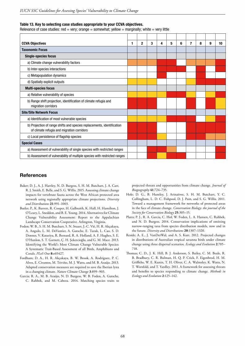
68

IUCN SSC Guidelines for Assessing Species’ Vulnerability to Climate Change

References

Baker; D. J., A. J. Hartley, N. D. Burgess, S. H. M. Butchart, J. A. Carr, R. J. Smith, E. Belle, and S. G. Willis. 2015. Assessing climate change impacts for vertebrate fauna across the West African protected area network using regionally appropriate climate projections. Diversity and Distributions 21:991–1003.

Butler; P., K. Barrett, R. Cooper, H. Galbraith, K. Hall, H. Hamilton, J. O’Leary, L. Sneddon, and B. E. Young. 2014. Alternatives for Climate Change Vulnerability Assessment: Report to the Appalachian Landscape Conservation Cooperative. Arlington, Virginia.

Foden; W. B., S. H. M. Butchart, S. N. Stuart, J.-C. Vié, H. R. Akçakaya, A. Angulo, L. M. DeVantier, A. Gutsche, E. Turak, L. Cao, S. D. Donner, V. Katariya, R. Bernard, R. A. Holland, A. F. Hughes, S. E. O’Hanlon, S. T. Garnett, Ç. H. Şekercioğlu, and G. M. Mace. 2013. Identifying the World’s Most Climate Change Vulnerable Species: A Systematic Trait-Based Assessment of all Birds, Amphibians and Corals. PLoS One 8:e65427.

Fordham; D. A., H. R. Akçakaya, B. W. Brook, A. Rodríguez, P. C. Alves, E. Civantos, M. Triviño, M. J. Watts, and M. B. Araújo. 2013. Adapted conservation measures are required to save the Iberian lynx in a changing climate. Nature Climate Change 3:899–903.

Garcia; R. A., M. B. Araújo, N. D. Burgess, W. B. Foden, A. Gutsche, C. Rahbek, and M. Cabeza. 2014. Matching species traits to

projected threats and opportunities from climate change. Journal of Biogeography 41:724–735.

Hole; D. G., B. Huntley, J. Arinaitwe, S. H. M. Butchart, Y. C. Collingham, L. D. C. Fishpool, D. J. Pain, and S. G. Willis. 2011. Toward a management framework for networks of protected areas in the face of climate change. Conservation Biology: the journal of the Society for Conservation Biology 25:305–15.

Platts; P. J., R. A. Garcia, C. Hof, W. Foden, L. A. Hansen, C. Rahbek, and N. D. Burgess. 2014. Conservation implications of omitting narrow-ranging taxa from species distribution models, now and in the future. Diversity and Distributions 20:1307–1320.

Reside; A. E., J. VanDerWal, and A. S. Kutt. 2012. Projected changes in distributions of Australian tropical savanna birds under climate change using three dispersal scenarios. Ecology and Evolution 2:705–718.

Thomas; C. D., J. K. Hill, B. J. Anderson, S. Bailey, C. M. Beale, R. B. Bradbury, C. R. Bulman, H. Q. P. Crick, F. Eigenbrod, H. M. Griffiths, W. E. Kunin, T. H. Oliver, C. A. Walmsley, K. Watts, N. T. Worsfold, and T. Yardley. 2011. A framework for assessing threats and benefits to species responding to climate change. Methods in Ecology and Evolution 2:125–142.

Table 13. Key to selecting case studies appropriate to your CCVA objectives. Relevanceofcasestudies:red=very;orange=somewhat;yellow=marginally;white=verylittle

CCVA Objectives 1 2 3 4 5 6 7 8 9 10

Taxonomic Focus

Single-species focus

a)Climatechangevulnerabilityfactors

b)Inter-speciesinteractions

c)Metapopulationdynamics

d)Spatiallyexplicitoutputs

Multi-species focus

a)Relativevulnerabilityofspecies

b)Rangeshiftprojection,identificationofclimaterefugiaand migrationcorridors

Site/Site Network Focus

a)Identificationofmostvulnerablespecies

b)Projectionofrangeshiftsandspeciesreplacements,identification ofclimaterefugiaandmigrationcorridors

c)Localpersistenceofflagshipspecies

Special Cases

a)Assessmentofvulnerabilityofsinglespecieswithrestrictedranges

b)Assessmentofvulnerabilityofmultiplespecieswithrestrictedranges

69

CaseStudy1.AcorrelativeapproachforAustraliantropicalsavannabirds By: April ResideBased on: Reside et al., 2012

1.OverallobjectivesIn tropical eastern Australia, work had been done investigating the likely impact of climate change on tropical rainforest fauna. However, no studies had been conducted on the habitats that make up the vast majority of tropical Australia – tropical savannas. This study began to address this gap by focusing on tropical savanna birds, as birds were the best surveyed taxonomic group and therefore had the most comprehensive datasets.

Summary of the CCVA objectivesObjectives 1.Investigatetheimpactofclimate

changeontheamountandlocationofsuitableclimatespaceforspecies

2.Investigatetheimpactofdifferentdispersalscenariosonfutureprojectionsofspeciesdistributions

3.Estimatethechangeinspeciesrichnessfrombaselineto2080usingmodelledprojectionsofspeciesdistributionsandrealisticdispersalscenarios

Taxonomicfocus BirdsGeographicFocus AustraliantropicalsavannasTimeframe Frombaseline(1990)to2080

2.ContextTropical savannas make up nearly a quarter of mainland Australia, extending from the eastern coast across the continent to the western and northern coasts. The tropical savannas are characterized by highly variable annual rainfall, to which occupying species have adapted by having low dietary specificity or by being highly mobile and thereby able to track shifting resources. Generally speaking, savanna biota is thought to be robust in the face of environmental change, due to being widespread and occurring with highly variable conditions. However, evidence of decline of many mammal and bird species in this region has been accumulating, causing conservation agencies to question this widely held belief. Further investigation was needed to understand how savanna species were likely to be impacted by climate change. Furthermore, the understanding of how species within key biogeographic regions within the savannas were similarly impacted by climate change was needed to focus conservation attention.

The Australian Federal Government’s lead research organization, CSIRO, and James Cook University funded a project to: 1) develop species distribution modelling methods appropriate for use on highly mobile species in a highly variable environment; and 2) model the species’ distributions under different climate change scenarios.

3.RationaleforapproachandmethodsWe selected a correlative approach to examine climate change vulnerability. Firstly we modelled the species’ distributions under climate change scenarios and investigated the resulting projections of suitable climate space, and how these varied with different dispersal scenarios. In a second, separate and as yet unpublished step, we combined these correlative models with a trait-based approach to generate a comprehensive comparative climate change vulnerability analysis.

Suitability of methodsCorrelative Trait-based Mechanistic Combined

Meetsobjectives?

Yes Yes Possibly Yes

Resourcesavailable?

Yes Yes No Yes

Selected? Yes Yes(separatestudy)

No Forafollow-upassessment

We selected Maxent (Phillips et al., 2006) for carrying out correlative modelling because collaborators were involved in the species distribution modelling method evaluation which found Maxent to be the strongest performing algorithm among those tested (Elith et al., 2006). We were provided use of James Cook University’s High Performance Computing Cluster which allowed us to carry out parallel modelling of hundreds of species and multiple future scenarios in a relatively short time. The modelling involved 243 bird species, three emissions scenarios (SRES A2, A1B and B1) (Nakicenovic et al., 2000), 30 General Circulation Models (GCM) (Cubash et al., 2001) and ten time slices; equating to 218,700 outputs, which required approximately 13 years of parallel processing.

4.ApplicationofmethodsBirds were chosen as a focus because most of the data for savanna biota are for birds, and because of evidence of decline in some of the bird foraging guilds in this region. Trait-based data are available for most Queensland species, so this study examined Queensland savanna bird species for which suitable data were available. The main occurrence data source was BirdLife Australia, which has now shared the data with Atlas of Living Australia. Data on species dispersal abilities were compiled from the literature, and from data collected by CSIRO’s savanna biodiversity research team. Many months of work was involved in vetting the species occurrence data, involving the removal of obviously erroneous records. The climate data were obtained from the Australian Water Availability Project (Grant et al., 2008, Jones et al., 2007), and the climate layers were created using the “climates” package in R (VanDerWal et al., 2011a). Model post processing was done using the “SDMTools” package in R (VanDerWal et al., 2011b). While access to James Cook University’s High Performance Computing Cluster made this work possible, processing the large input datasets and high volume of output models was challenging. Having access to the modelling

10. Case studies

70

IUCN SSC Guidelines for Assessing Species’ Vulnerability to Climate Change

Peninsula were projected to lose the most suitable climate space across all species. These species are likely to be particularly vulnerable because of their small distributions (particularly in comparison to other species) and the alteration of fire regimes in recent decades (Reside et al., 2012a).

This study found that the dispersal scenario used for calculating the amount of suitable climate space into the future can dramatically change the predicted outcomes for species. In particular, comparing the extremes from unlimited dispersal (i.e. a species is able to disperse as far as required in order to track suitable climate) to no dispersal (i.e. species would only be able to occupy suitable climate space in the future if it overlapped currently suitable areas) show completely different stories, from substantial increases in species to substantial decreases. Neither scenario is likely to be accurate, as many species are already more restricted than their modelled climate envelope and there is a lot of evidence of birds dispersing outside of their historic range in recent years. Tailoring dispersal scenarios to individual species dispersal abilities is important for having more accurate projections of climate change impacts.

6.ConservationoutcomesThese results were disseminated through publication of the research paper in a scientific journal (Reside et al., 2012) and presentations at various conferences and seminars, including PhD pre-completion seminars, lab seminars at the Durrell Institute of Conservation Ecology at Kent University in the UK and La Sapienza University in Rome, and the Ecological Society of Australia annual conferences. The results from this study may have had little uptake; however, the modelling methods were subsequently applied to 2,000 vertebrate species across Australia in a follow-up study (Reside et al., 2013), and these results have had widespread use and uptake. The main stakeholders interested in these results include state governments across Australia, Natural Resource Management groups and other researchers. The results of these studies have been incorporated into climate change adaptation plans for the Natural Resource Management groups and in land acquisition for the National Reserve System.

7.RoomforimprovementThis study and the subsequent studies (Reside et al., 2013) could be improved by evaluating the impact of using the chosen modelling algorithm (Maxent) on the projected outcomes. Furthermore, fully understanding how species will respond to climate change will require information on individual species’ sensitivity to change and their adaptive capacity. Work on incorporating these factors into the vulnerability of savanna birds to climate change has been conducted, and is currently in review for publication (Reside et al., in review). When this work began, few if any frameworks for trait-based approaches were available. As a result, it proved exceedingly difficult to convince reviewers of the validity of combining correlative-modelling and trait-based approaches to assess species vulnerability to climate change. For this reason, this study with the combined

support of Assoc. Prof. Jeremy VanDerWal at JCU was essential for the success of this project.

A challenge encountered was how to present and create a coherent story from the >200,000 outputs. After various iterations, it was decided to only present the outputs from the moderately severe emissions scenario modelled (SRES A1B) because this enabled a more coherent narrative of the results, and it was a mid-range scenario. We believe this is justified because the outputs from the various emissions scenarios did not influence the direction of change, or the spatial realization of change. Only the length of time taken to reach a specific outcome varied.

In the paper, a mean projection for each time slice was presented for A1B for species. These projected distributions were converted to binary ‘suitable’/’not suitable’ using a Maxent-derived threshold of suitability; these thresholded binary outputs were summed to give an estimate of species richness for each time slice. This was done for each of the different dispersal scenarios so the results could be compared.

The outputs consisted of a modelled distribution for each combination of species, emissions scenario, GCM and time slice. From this, mean projections for each species, time slice and emissions scenario were generated. These were later incorporated into the trait-based analysis, which is still in review.

We examined how species with different migration/movement strategies were likely to fare under climate change. We compared the amount of future climate space projected to remain suitable for species that were migratory, nomadic, partially migratory, sedentary, or species with both nomadic and sedentary populations. Many of the species in our study also occurred widely outside the savanna region; e.g., some occurring along the mesic east coast and some occupying both savanna and arid regions. We compare the amount of projected future suitable climate space between species with different biogeographic affiliations. Finally, we examined the amount of climate space projected to remain suitable for species that were listed as threatened under state, federal and international conservation listings.

5.SummaryofresultsMigratory species and those mainly confined to tropical environments were projected to lose the least suitable climate space by 2080, and in fact some species confined to tropical environments were predicted to see a substantial increase in suitable climate space by 2080 (Reside et al., 2012b). This was largely driven by the projections for increases in rainfall in the centre of the tropical savanna area. These projections for the future are likely to be realized to some extent, as conditions for savanna birds in this area have been shown to improve due to increases in rainfall in the past 60 years (VanDerWal et al., 2013). However, the tropical species confined to Cape York

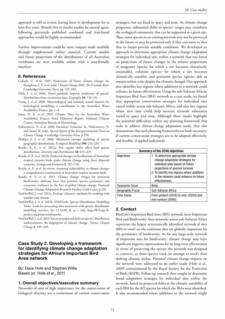
71

approach is still in review, having been in development for at least five years. Should this or similar studies be started again, following previously published combined and trait-based approaches would be highly recommended.

Further improvements could be more outputs made available through supplemental online material. Current models and future projections of the distributions of all Australian vertebrates are now available online with a user-friendly interface.

8.ReferencesCubash, U. et al. 2001. Projections of future climate change. In:

Houghton, J. T. et al. (eds), Climate Change 2001: The Scientific Basis. Cambridge University Press, pp. 525–582.

Elith, J. et al. 2006. Novel methods improve prediction of species’ distributions from occurrence data. Ecography 29: 129–151.

Grant, I. et al. 2008. Meteorological and remotely sensed datasets for hydrological modelling: a contribution to the Australian Water Availability Project. pp. 1–4.

Jones, D. A. et al. 2007. Climate Data for the Australian Water Availability Project: Final Milestone Report. National Climate Centre, Australian Bureau of Meteorology.

Nakicenovic, N. et al. 2000. Emissions Scenarios. In: Nakicenovic, N. and Swart, R. (eds), Special Report of the Intergovernmental Panel on Climate Change. Cambridge University Press, p 570.

Phillips, S. J. et al. 2006. Maximum entropy modeling of species geographic distributions. Ecological Modelling 190: 231–259.

Reside, A. E. et al. 2012a. Fire regime shifts affect bird species distributions. Diversity and Distributions 18: 213–225.

Reside, A. E. et al. 2012b. Projected changes in distributions of Australian tropical savanna birds under climate change using three dispersal scenarios. Ecology and Evolution 2: 705–718.

Reside, A. E. et al. In review. Assessing vulnerability to climate change: a comprehensive examination of Australian tropical savanna birds.

Reside, A. E. et al. 2013. Climate change refugia for terrestrial biodiversity: defining areas that promote species persistence and ecosystem resilience in the face of global climate change. National Climate Change Adaptation Research Facility, Gold Coast, p 216.

VanDerWal, J. et al. 2011a. Package ‘climates’: methods for working with weather and climate.

VanDerWal, J. et al. 2011b. SDMTools: Species Distribution Modelling Tools: Tools for processing data associated with species distribution modelling exercises. In: 1.1-5/r90, R. p. v. (ed), http://R-Forge.R-project.org/projects/sdmtools/.

VanDerWal, J. et al. 2013. Focus on poleward shifts in species’ distribution underestimates the fingerprint of climate change. Nature Climate Change 3: 239–243.

CaseStudy2.DevelopingaframeworkforidentifyingclimatechangeadaptationstrategiesforAfrica’sImportantBirdAreanetwork

By: Dave Hole and Stephen WillisBased on: Hole et al., 2011

1.Overallobjectives/executivesummaryNetworks of sites of high importance for the conservation of biological diversity are a cornerstone of current conservation

strategies, but are fixed in space and time. As climate change progresses, substantial shifts in species’ ranges may transform the ecological community that can be supported at a given site. Thus, some species in an existing network may not be protected in the future or may be protected only if they can move to sites that in future provide suitable conditions. We developed an approach to determine appropriate climate change adaptation strategies for individual sites within a network that was based on projections of future changes in the relative proportions of emigrants (species for which a site becomes climatically unsuitable), colonists (species for which a site becomes climatically suitable), and persistent species (species able to remain within a site despite the climatic change). Our approach also identifies key regions where additions to a network could enhance its future effectiveness. Using the sub-Saharan African Important Bird Area (IBA) network as a case study, we found that appropriate conservation strategies for individual sites varied widely across sub-Saharan Africa, and that key regions where new sites could help increase network robustness varied in space and time. Although these results highlight the potential difficulties within any planning framework that seeks to address climate-change adaptation needs, they also demonstrate that such planning frameworks are both necessary, if current conservation strategies are to be adapted effectively, and feasible, if applied judiciously.

Summary of the CCVA objectivesObjectives 1.Todetermineappropriateclimate

changeadaptationstrategiesforindividualsitesbasedonfutureprojectionsofspeciesturnover.

2.Toidentifykeyregionswhereadditionstothenetworkcouldenhanceitsfutureeffectiveness.

Taxonomicfocus BirdsGeographicFocus Sub-SaharanAfricaTimeframe Frompresent(2010)tomid-(2050)and

end-century(2080)

2.ContextBirdLife’s Important Bird Area (IBA) network (now Important Bird and Biodiversity Area network) across sub-Saharan Africa represents the largest systematically identified network of sites (803 in total) on the continent that are globally important for the persistence of biodiversity. As for any large-scale network of important sites for biodiversity, climate change may have significant negative repercussions for its long-term effectiveness in terms of preserving the species the network was designed to conserve, as those species track (or attempt to track) their shifting climatic niches. Potential climate change impacts on the network were addressed in an earlier study (Hole et al., 2009) commissioned by the Royal Society for the Protection of Birds (RSPB). Follow-up research then sought to determine broad adaptation strategies for individual sites within the network, based on projected shifts in the climatic suitability of each IBA for the 815 species for which the IBAs were identified. It also recommended where additions to the network might

10. Case studies

72

IUCN SSC Guidelines for Assessing Species’ Vulnerability to Climate Change

increase its effectiveness under a changing climate. Durham University (UK), a leading institution in the assessment of climate change impacts on biodiversity, carried out the work, in collaboration with BirdLife International and RSPB.

3.RationaleforapproachandmethodsGiven the large taxonomic and geographic scope of this case study (815 species, all of sub-Saharan Africa), correlative methods were selected. Data limitations for most of these species precluded the use of mechanistic modelling, while trait-based assessments would have been inadequate for providing the necessary spatial component to understand heterogeneity in climatic suitability of individual IBAs. Fortunately, locality data for all species of interest were available from the University of Copenhagen at sufficient (though not ideal) spatial resolution, making the correlative approach particularly appealing.

Suitability of methodsCorrelative Trait-based Mechanistic Combined

Meetsobjectives?

Yes No Yes Yes

Resourcesavailable?

Yes No No No

Selected? Yes No No No

Climate Response Surface (CRS) models were selected for their previously demonstrated utility in modelling projected climate impacts on birds (Huntley et al., 2006b). Generalized Additive Models (GAMs) were also applied in order to assess uncertainty resulting from modelling methodology.

In order to meet the goals of our case study, our primary need was to develop an understanding of how priority bird species might change in terms of their representation (i.e. either disappear from, colonise, or continue to persist in) individual IBAs across the entire sub-Saharan African IBA network, as a result of climate change. Correlative models, despite their acknowledged limitations (e.g., Pacifici et al., 2015) provided us with a methodology that enabled us to project presence/absence within individual IBAs over time, across a large number of species. Our resulting framework describing climate change adaptation strategies for all sites in the network based on this broad suite of species (see below), was therefore more robust to bias resulting from a few poorly fitted models, than if we had based it on a handful of species-specific projections for individual IBAs.

4.ApplicationofmethodsWe assessed all (815) “priority” species (i.e. those that trigger IBA designation) in sub-Saharan Africa, because it is shifts in their distributions and representation within IBAs that could most impact the future efficacy of the network under climate change. They include all globally threatened, restricted range and biome-restricted species (note that we excluded the small number of congregatory species that also trigger IBA designation).

Data for modelling of all 815 species were obtained from the Zoological Museum of the University of Copenhagen at one-degree resolution. This was the most reliable and comprehensive dataset available at the time. ‘Current’ climate data were obtained from Worldclim (http://www.worldclim.org) at 2.5’ resolution and aggregated to 10. Future climate data were obtained from the IPCC’s data archive (Third Assessment Report). Significant computational resources were required to downscale and combine the current climate data with the future anomalies (note that these analyses were conducted in 2007 and future climate scenarios are now readily available). Uniquely, we were able to validate our modelling approach by comparing modelled IBA species inventories with current community composition of a sub-set of IBAs for which we had ‘observed’ data, based on actual species lists. Such observed data, while critical for model validation, are a major challenge to obtain and were only available as a result of BirdLife International’s extensive contacts with local organizations in the region.

Models were developed for each of the 815 species using point locality data and four bioclimatic variables (selected for their previously demonstrated utility in modelling avian distributions; Huntley et al., 2006b) covering the entire sub-Saharan African region. Each species model was then projected onto individual climates characterized for each IBA, for the present and for three future climate projections (derived from three separate General Circulation Models that capture the range of variability in future projections of precipitation (Hole et al., 2009)) and two future time periods (centred on 2055 and 2085). Modelled current and projected future probabilities of occurrence were then used to generate current and future ‘expected’ species inventories for each IBA. These modelled inventories were then validated against the ‘observed’ species lists for our subset of IBAs, indicating adequate robustness for us to move forward. For each IBA, models for the 815 species, for the present and future time periods, were then used to estimate the proportions of colonizers (species for which a currently unsuitable IBA becomes suitable in the future), emigrants (species for which an IBA that is currently suitable becomes unsuitable in the future) and persistent species (species for which an IBA that is suitable in the present remains suitable in the future). Finally, climate change adaptation strategies for each site within the network were defined, based on the relative proportions of each of these three groupings of species within each IBA. We also used the models generated for the 815 species to evaluate where additions to the network could facilitate range shifts and fill gaps, by identifying: i) regions that our models suggested would be most important in the future for priority species least well supported by the existing network; ii) regions into which large numbers of priority species are projected to move; and iii) regions that are least well covered by the existing network (based simply on the distance from each 0.250 grid cell in sub-Saharan Africa to the nearest IBA).

73

5.SummaryofresultsThe framework synthesising model projections for all 815 species for assigning high level adaptation strategies for individual sites is quite simple. We calculated mean proportions of projected emigrant and colonist priority species for each IBA, for each period, as the mean of the values for the three future projections. We then plotted the ensemble mean proportion of projected emigrants against the ensemble mean proportion of projected colonists for each IBA. We used the median, lower quartile, and upper quartile of values along each axis to divide the area of the resulting graph into five sectors (Figure CS 2.1).

Figure CS 2.1. Schematic showing how IBAs (red dots) were allocated to one of five categories, based on their respective proportions of emigrants, colonists and persistent species (derived from Hole etal., (2011)).

Finally, we classified each IBA into one of five categories according to the graph sector into which it fell: high persistence, increasing specialization, high turnover, increasing value, and increasing diversification. We then used the character of the projected changes in the proportions of emigrant, colonist, and persistent priority species in each category to identify general principles for the CCAS most appropriate for IBAs in that category, recognizing the contribution made by each category to achieving the goals of the entire network. We inferred changes in the proportion of persistent species from the proportion of emigrants (if the proportion of emigrants was high, the proportion of persistent species must, by definition, be low, and vice versa). We also determined the category-specific relevance of the likely need to adopt management actions that promote resistance (forestall effects and protect highly valued resources), resilience (improve capacity to return to desired conditions after disturbance), or facilitation (facilitate transition from current to new conditions). Finally, for each category, we determined the character and relative importance of five key management actions (drawn from Heller & Zavaleta, (2009), Mawdsley et al., (2009), Millar et al., (2007), and Galatowitsch et al., (2009)) aimed at enhancing the adaptive capacity of a site’s complement of priority species: habitat restoration and creation; disturbance regime management; translocation; increase in site extent; and matrix management.

Additionally, we combined our three indicators of where additional sites could add to future network resilience into

a single index of ‘added value’ and mapped it across sub-Saharan Africa.

Sites in the high persistence and high turnover categories were twice as common as the other three categories. The distribution of site categories was strongly geographically patterned. In particular, the high persistence category predominated in the Guinea–Congo region and much of West Africa, whereas the high turnover category predominated in the southern African tropical zone (stretching from Namibia and Angola to Mozambique and Tanzania). Elsewhere, for example, in northern east Africa (Ethiopia, Somalia, Kenya and Uganda) and in South Africa, no one category predominated. Larger increasing value IBAs were principally on the Saharan margin (Niger, Chad, and Sudan) or in the arid southwest (primarily Namibia). Smaller IBAs in this category were widely scattered. In terms of potentially optimal locations for additional sites, these were located primarily in Gabon, Congo, Namibia, Botswana, eastern South Africa, southern Mozambique, and from Tanzania through the Albertine Rift north to Ethiopia and Somalia.

6.ConservationoutcomesResults were disseminated through the peer-review literature, through presentation of the results at international conferences and at BirdLife Partnership meetings, and through the Partnership’s extranet website. As BirdLife Partners (particularly those in developing countries) move towards developing and implementing coherent strategies for climate change adaptation, the Hole et al., (2011) approach is unique in providing generic guidance on adaptation actions to implement, that are informed by projected impacts at the scale of individual sites.

7.RoomforimprovementFiner resolution species distribution data and mechanistically down-scaled climate data (i.e. using a regional climate model rather than the simple statistical approach used here) would have improved the robustness of our results – yet such data were simply not available at the time, and still aren’t at the pan-African scale.

More broadly, there is a need to better integrate into funding proposals and project planning, the financial resources and activities needed for translating the content of published scientific papers into adaptation guidance that is carefully targeted at relevant constituencies (e.g. site managers), as well as the resources for dissemination.

8.ReferencesGalatowitsch; S., L. Frelich, and L. Phillips-Mao. 2009. Regional

climate change adaptation strategies for biodiversity conservation in a midcontinental region of North America. Biological Conservation 142:2012–2022.

Heller; N. E., and E. S. Zavaleta. 2009. Biodiversity management in the face of climate change: A review of 22 years of recommendations. Biological Conservation 142:14–32.

10. Case studies

74

IUCN SSC Guidelines for Assessing Species’ Vulnerability to Climate Change

Hole; D. G., B. Huntley, J. Arinaitwe, S. H. M. Butchart, Y. C. Collingham, L. D. C. Fishpool, D. J. Pain, and S. G. Willis. 2011. Toward a management framework for networks of protected areas in the face of climate change. Conservation Biology: the Journal of the Society for Conservation Biology 25:305–15.

Hole; D. G., S. G. Willis, D. J. Pain, L. D. Fishpool, S. H. M. Butchart, Y. C. Collingham, C. Rahbek, and B. Huntley. 2009. Projected impacts of climate change on a continent-wide protected area network. Ecology Letters 12:420–31.

Huntley; B., Y. C. Collingham, R. E. Green, G. M. Hilton, C. Rahbek, and S. G. Willis. 2006a. Potential impacts of climatic change upon geographical distributons of birds. Ibis 148:8–28.

Huntley; B., Y. C. Collingham, R. E. Green, G. M. Hilton, C. Rahbek, and S. G. Willis. 2006b. Potential impacts of climatic change upon geographical distributions of birds. Ibis 148:8–28.

Mawdsley; J. R., R. O’Malley, and D. S. Ojima. 2009. A review of climate-change adaptation strategies for wildlife management and biodiversity conservation. Conservation Biology 23:1080–1089.

Millar; C. I., N. L. Stephenson, and S. L. Stephens. 2007. Climate change and forest of the future: Managing in the face of uncertainty. Ecological Applications 17:2145–2151.

Pacifici; M., W. B. Foden, P. Visconti, J. E. M. Watson, S. H. M. Butchart, K. M. Kovacs, B. R. Scheffers, D. G. Hole, T. G. Martin, H. R. Akçakaya, R. T. Corlett, B. Huntley, D. Bickford, J. A. Carr, A. A. Hoffmann, G. F. Midgley, P.-K. P., R. G. Pearson, S. E. Williams, S. G. Willis, B. Young, and C. Rondinini. 2015. Assessing species vulnerability to climate change. Nature Climate Change 5:215–225.

CaseStudy3.BacktobasicswithAfricanamphibians

By: Philip J. Platts and Raquel A. GarciaBased on: Platts et al., 2014a

1.OverallobjectivesFor CCVAs employing correlative techniques such as species distribution modelling (SDM), a particular challenge is that species with insufficient numbers of occurrence records cannot be modelled. Depending on the scale of analysis, this can mean leaving out many range-restricted species, which are typically the ones of highest conservation concern (Schwartz et al., 2006, Platts et al., 2014a).

Does this omission of range-restricted species matter, when assessing spatial patterns of vulnerability across a higher taxonomic rank? If either of the following hypotheses is correct, then the answer is likely to be yes: (1) species omitted from correlative SDM have, on average, different climatic niches to those species eligible for modelling; (2) omitted species and eligible species are projected to experience different climate anomalies in the future.

Summary of the CCVA objectivesObjectives 1.Totesthypothesesaboutlarge-scale

conservationpriorityschemes.2.ToassessspatialbiasinCCVAresults.

Taxonomicfocus Amphibians

Geographicfocus MainlandAfricasouthoftheSahara

Timeframe Late-20thcenturythroughlate21stcentury

2.ContextCorrelative models that predict species distributions under climate change are frequently applied in the scientific literature, and are widely cited by conservation planners seeking to determine whether existing priorities will remain valid under future climates. Such models must be underpinned by sufficient data on a species’ distribution to avoid spurious predictions (Stockwell and Peterson 2002) – a prerequisite that is, almost by definition, not fulfilled by many species of highest conservation concern, particularly at the coarse spatial resolutions dictated by commonly available species and climate data at continental scales.

This is especially true in the tropics, where species are more often narrow-ranging than at higher latitudes (Wiens et al., 2006), and even common species’ distributions tend to be less well documented (Feeley and Silman 2011). These data challenges are exemplified in sub-Saharan Africa, where species information is patchy at best, and confounded by spatial uncertainties in historical records.

In light of these obstacles, it is worthwhile considering how the omission of range-restricted (or under-sampled) species from familiar SDM tools might bias CCVA results. Amphibians were chosen as a case study due to the high levels of threat they face from climate change, habitat loss and disease (Sodhi et al., 2008, Hof et al., 2011). Amphibians native to Africa are mostly endemic to the continent, making the modelling more tractable.

3.RationaleforapproachandmethodsOf the three main options for CCVA, correlative approaches are by far the most commonly applied. Mechanistic methods are rarely feasible for large groups of under-studied species. Trait-based assessments are a viable alternative (Foden et al., 2013) and could be integrated with correlative approaches (Garcia et al., 2014, Willis et al., 2015). Here though, the objective was to determine the implications of restricting CCVA to correlative techniques.

To test the hypotheses that species omitted from SDM occupy different climatic niches and/or face different exposures to climate change, it was sufficient to perform multivariate ordination on the species’ point distributions. Inferring modelled patterns of vulnerability or future priority for omitted species, however, given their stated omission from the modelling procedure in question, is clearly troublesome. To evade this catch-22, it was necessary to redefine SDM in terms of its most basic interpretation (Busby 1991), and thence to modify the procedure such that any species, irrespective of range-size, could be included in the analysis (see below).

75

Suitability of methodsCorrelative Trait-based Mechanistic Combined

Meetsobjectives?

Yes No No No

Resourcesavailable?

Yes Yes No No

Selected? Yes No No No

4.ApplicationofmethodsDistributional data were gathered for 790 species of amphibians found only on mainland Africa south of the Sahara (Hansen et al., 2007; updated to February 2014). Matching to IUCN taxonomy (www.iucnredlist.org) reduced the number of species to 733. The data are reliable to 1° resolution (111 km at the equator). Each amphibian was deemed either eligible for, or omitted from, correlative SDM based on a ten record cut-off (thresholds in other studies range from five to 50 records). Multivariate ordination (Outlying Mean Index, OMI; Dolédec et al. 2000) tested for differences in observed distributions between eligible versus omitted species, in terms of (1) climatic niche space and (2) projected exposure to change (climate anomalies).

Climate was summarized by four, weakly collinear (Pearson’s |r|<0.7) variables: mean temperature and annual temperature range, mean rainfall and rainfall seasonality. Baseline conditions (1950-2000) were from WorldClim (Hijmans et al., 2005), using mean values to resample from 30” to 1° resolution. Future conditions (2071–2100) were from AFRICLIM: regionally-downscaled CMIP5 GCMs, debiased against the WorldClim baselines (Platts et al., 2015). Two IPCC-AR5 emissions pathways were considered: RCP4.5 and RCP8.5. For temperature variables, future anomalies were computed by subtracting the future from the present values; anomalies for rainfall variables were given by the ratio of future to present.

All amphibian distributions were projected in space and time using multidimensional niche envelopes (MDNE). Unlike modern SDM methods, this simple technique classifies all conditions within a species’ observed climatic range as uniformly viable, and conditions beyond as wholly unsuitable. So as to include even those amphibians with a single occurrence record, the interquartile range of local (30”) climatic conditions within the 1° grid cell(s) was used to define the envelopes. Future predictions were constrained under a no-dispersal scenario (climate change velocities at 1° resolution are expected to outpace dispersal capabilities for most African amphibians).

5.SummaryofresultsOf the 733 amphibian species, 400 have too few records for correlative SDM, including 92% of those threatened with extinction (VU/EN/CR on The IUCN Red List). Species omitted from SDM occupy significantly different niche space to eligible species: their observed distributions are characterized by higher annual rainfall with lower rainfall seasonality, cooler and less seasonal temperatures, and by more complex

topography. This is consistent with a wider literature on the broad-scale tendency for climatically and topographically diverse/distinct areas to contain a disproportionate richness of narrow-ranging species (Ohlemüller et al., 2008).

Empirically-derived priority metrics (e.g., top 100 cells for species richness) were derived for each species set (eligible or omitted) and time-period (present or future), by stacking the modelled species distributions. These metrics were compared against three large-scale conservation priority schemes: Conservation International’s Biodiversity Hotspots (Mittermeier et al., 2004), BirdLife International’s Endemic Bird Areas (Stattersfield et al., 1998) and the World Wildlife Fund’s Global 200 ecoregions (Olson and Dinerstein 1998).

Congruence between empirical priority metrics and existing schemes was generally higher on the omitted species set than on the eligible species set, although this varied depending on the region and metric considered. Projecting empirical metrics under future climate, congruence with existing schemes reduced in western Africa while generally increasing in eastern and southern Africa. Overall, priorities for eligible species were projected to shift towards existing schemes (and thus towards omitted species), due to greater climatic stability at these sites. Similarly, while omitted species frequently lost all climate space at 1° resolution, persistent populations tended to coincide with existing priority schemes. These results are summarized in Figure CD3.1.

6.ConservationoutcomesUnder current climate, data thresholds imposed by SDM systematically downplay important sites for narrow-ranging and threatened species. This issue spans taxonomic groups and is only partially mitigated by modelling at finer scales. Under future climate, persistence among both narrow- and wide-ranging species may (depending on finer-scale processes) be highest within sites already identified for conservation investment, and so the focus on these sites ought to be maintained.

The results of this study were distributed through a journal article (Platts et al., 2014) and associated media coverage (e.g., http://www.unep-wcmc.org/news/near-extinct-african-amphibians-invisible-under-climate-change), facilitated by wildlife photography to engage a broader audience (www.michelemenegon.it/).

7.RoomforimprovementThe ‘back to basics’ envelope models used here, while useful for demonstrating potentially contrasting model outcomes for narrow- versus wide-ranging species, should not be seen as sufficient in addressing the rare species problem. Rather, a wider range of approaches, encompassing trait-based, mechanistic and correlative procedures (and combinations of these) should be developed and deployed in CCVAs, in order that the vulnerability of range-restricted species can be adequately represented in conservation plans.

10. Case studies

76

IUCN SSC Guidelines for Assessing Species’ Vulnerability to Climate Change

8.ReferencesBusby; J. R. 1991. BIOCLIM – a bioclimatic analysis and prediction

system. Pages 64–68 in C. R. Margules and M. P. Austin, editors. Nature Conservation: Cost Effective Biological Surveys and Data Analysis. CSIRO, East Melbourne, Australia.

Dolédec; S., D. Chesse, and C. Gimaret-Carpentier. 2000. Niche separation in community analysis: a new method. Ecology 81:2914–2927.

Feeley; K. J. and M. R. Silman. 2011. The data void in modeling current and future distributions of tropical species. Global Change Biology 17:626–630.

Foden; W. B., S. H. M. Butchart, S. N. Stuart, J.-C. Vié, H. R. Akçakaya, A. Angulo, L. M. DeVantier, A. Gutsche, E. Turak, L. Cao, S. D. Donner, V. Katariya, R. Bernard, R. A. Holland, A. F. Hughes, S. E. O’Hanlon, S. T. Garnett, Ç. H. Şekercioğlu, and G. M. Mace. 2013. Identifying the World’s Most Climate Change Vulnerable Species: A Systematic Trait-Based Assessment of all Birds, Amphibians and Corals. PLoS One 8:e65427.

Garcia; R. A., M. B. Araújo, N. D. Burgess, W. B. Foden, A. Gutsche, C. Rahbek, and M. Cabeza. 2014. Matching species traits to projected threats and opportunities from climate change. Journal of Biogeography 41:724–735.

Hansen, L.A., Burgess, N.D., Fjeldså, J., Rahbek; C. 2007. One degree resolution databases of the distribution of 739 amphibians in sub-Saharan Africa (version 1.0). Zoological Museum, University of Copenhagen, Copenhagen, Denmark.

Hijmans; R. J., S. E. Cameron, J. L. Parra, P. G. Jones, and A. Jarvis. 2005. Very high resolution interpolated climate surfaces for global land areas. International Journal of Climatology 25:1965–1978.

Hof; C., M. B. Araújo, W. Jetz, and C. Rahbek. 2011. Additive threats from pathogens, climate and land-use change for global amphibian diversity. Nature 480:516–519.

Mittermeier; R. A., P. R. Gil, M. Hoffmann, J. Pilgrim, T. Brooks, C. G. Mittermeier, J. Lamoreux, and G. A. B. da Fonseca. 2004. Hotspots Revisited: Earth’s Biologically Richest and Most Endangered Ecoregions. CEMEX, Mexico City, Mexico.

Figure CS3.1. For many amphibians in sub-Saharan Africa (and for other species groups), occurrence data are too scarce or spatially clustered for accurate species distribution modelling. This is particularly problematic for threatened species. The resulting bias against range-restricted species affects modelled estimates of richness, rarity and irreplaceability, both for current conditions and under climate change. Inset: Parker’s Forest Tree Frog (Leptopelis parkeri), Endangered on the IUCN Red List. Lower left: Barbour’s Forest Tree Frog (Leptopelis barbouri), Vulnerable. Background: mountain forests strip moisture from the air in Nyungwe National Park, Rwanda. Photography by Michele Menegon (www.michelemenegon.it). Composite reproduced from the cover of Diversity and Distributions, Vol. 20, Issue 11.

77

Ohlemüller; R., B. J. Anderson, S. H. M. Butchart, M. B. Arau, O. Kudrna, R. S. Ridgely, and C. D. Thomas. 2008. The coincidence of climatic and species rarity : high risk to small-range species from climate change. Biology Letters 4:568–572.

Olson; D. M., and E. Dinerstein. 1998. The Global 200: a representation approach to conserving the Earth’s most biologically valuable ecoregions. Conservation Biology 12:502–515.

Platts; P. J., R. A. Garcia, C. Hof, W. Foden, L. A. Hansen, C. Rahbek, and N. D. Burgess. 2014. Conservation implications of omitting narrow-ranging taxa from species distribution models, now and in the future. Diversity and Distributions 20:1307–1320.

Platts; P. J., P. A. Omeny, and R. Marchant. 2015. AFRICLIM: high-resolution climate projections for ecological applications in Africa. African Journal of Ecology 53:103–108.

Schwartz; M. W., L. R. Iverson, A. M. Prasad, S. N. Matthews, R. J. O’Connor, and O’Connor R. J. 2006. Predicting extinctions as a result of climate change. Ecology 87:1611–5.

Sodhi; N. S., D. Bickford, A. C. Diesmos, T. M. Lee, L. P. Koh, B. W. Brook, C. H. Sekercioglu, and C. J. a Bradshaw. 2008. Measuring the meltdown: drivers of global amphibian extinction and decline. PloS One 3:e1636.

Stattersfield, A., Crosby, M. J., Long, A. J. and Wege; D. C. 1998. Endemic Bird Areas of the world: priorities for biodiversity conservation. BirdLife International, Cambridge, UK.

Stockwell; D. R. B., and A. T. Peterson. 2002. Effects of sample size on accuracy of species distribution models. Ecological Modelling 148:1–13.

Wiens; J. J., C. H. Graham, D. S. Moen, S. a Smith, and T. W. Reeder. 2006. Evolutionary and ecological causes of the latitudinal diversity gradient in hylid frogs: treefrog trees unearth the roots of high tropical diversity. The American Naturalist 168:579–96.

Willis; S. G., W. Foden, D. J. Baker, E. Belle, N. D. Burgess, J. Carr, N. Doswald, R. A. Garcia, A. Hartley, C. Hof, T. Newbold, C. Rahbek, R. J. Smith, P. Visconti, B. E. Young, and S. H. M. Butchart. 2015. Integrating climate change vulnerability assessments from species distribution models and trait-based approaches. Biological Conservation 190:167–178.

CaseStudy4.ExploringimpactsofdecliningseaiceonpolarbearsandtheirringedsealandbeardedsealpreyinthenorthernBarentsSea

By: Robert C. Lacy, Kit M. Kovacs, Christian Lydersen and Jon Aars

1.OverallobjectivesClimate change is a major threat to polar bears, and extirpation (local extinction of populations) of this keystone arctic species is expected throughout much of the species range in the coming decades given current climate-gas emissions forecasts. The main effects of sea ice reductions due to global warming in the Arctic on the bears are caused by reduced availability of ice-associated seals, which are the primary prey of polar bears. These seals and the bears that prey on them are also important to coastal human populations throughout much of the Arctic. All of the ice-dependent seals breed only on sea ice, so availability of this unique habitat is directly linked to their reproductive success and ongoing existence; the carrying capacity for bears is in turn linked to these species. This case study is a novel exploration of

the impacts of a warming climate on the population trajectories of polar bears in combination with two of their key prey species – ringed and bearded seals – in the northern Barents Sea. The region is an arctic hot-spot that is experiencing rapid warming. We employed linked Population Viability Analysis (PVA) models to explore population trajectories of these three species out 100 years in order to inform management authorities and conservationists regarding the expected rates of decline within this species assemblage regionally.

Summary of the CCVA objectivesObjectives 1.Projectclimateimpactsthatcascade

throughpredator-preyrelationships.2.Understandwhencriticalchangesto

climateconditionsrequiredbyfocalspecieswilloccur.

3.Predictwhenclimatechangewilldrivepopulationstocriticallylowlevels.

Taxonomicfocus Polarbear,ringedseal,beardedsealGeographicFocus NorthernBarentsSeaTimeframe Frompresent(2010s)to2100s

2.ContextThis study was conducted because of concerns regarding the impacts that declining sea ice conditions are having on ice-dependent marine mammals in the Arctic (Laidre et al., 2008, 2015; Kovacs et al., 2011). We limited the scope of the study to the northern Barents Sea because it is a relatively data rich area for the species of concern and because it is a ‘hot spot’ with respect to environmental change due to climate warming. Additionally, it is a region that does not have aboriginal communities that are dependent on marine resources. Thus, management decisions can be made without subsistence hunting issues arising. Polar bears were selected as the focal species in this study (e.g., Hunter et al., 2010; Molnár et al., 2010) because they are a top predator that has strong influence on lower trophic levels and because they are a particularly sensitive management concern. Polar bear mothers require abundant, high-energy prey that is easily accessible from the land-fast ice (ice that makes contact with shore) in order to feed cubs when they emerge from dens in the spring after many months of fasting. This creates a critical dependency on the population of ringed seals that give birth to their pups in lairs (small snow caves) on the land-fast ice. Adult ringed seals and bearded seals are important prey for the polar bears throughout the year. Given the complexity of this system and the importance of these marine mammals to their ecosystems, the Norwegian Polar Institute and the Conservation Breeding Specialist Group sponsored collaboration among their scientists to pursue this study.

3.RationaleforapproachOur aim was to examine how impacts of climate change might cascade through the linkages among highly interdependent species. Most CCVA approaches are focused on single species, with the presumption that all other species with which they

10. Case studies

78

IUCN SSC Guidelines for Assessing Species’ Vulnerability to Climate Change

interact are either static or can be represented as simple trends in resources (prey) or threats (predators, competitors, or disease). However, if there are tight inter-relationships between species, including feedbacks between them, then models that project each species simultaneously, as well as their interactions, are needed for tests of the effects on the system of climate change or any major disruption to either species or to their interactions. We chose a metamodel approach to link PVAs, so that each PVA informs the other(s) about the dynamic changes in its focal species, and the functional relationships that link species are explicitly modelled. The approach of linking PVAs to explore how environmental changes can cause cascading effects through ecological dependencies of species has been used recently to examine threats due to disease (Shoemaker et al., 2014), landscape conversion to agriculture (Prowse et al., 2013), and invasive species (Miller et al., 2016). Here, we apply this methodology to the disruption of species inter-dependencies by climate change.

Suitability of methodsCorrelative Trait-based Mechanistic Combined

Meetsobjectives?

No No Yes No

Resourcesavailable?

Yes Yes Yes Yes

Selected? No No Yes No

For long-lived species, there may be considerable lags between the reduction in the environmental conditions that meet the habitat needs of a species and the consequent response in population numbers, especially when the mechanisms involved feedbacks between species. Therefore, correlative approaches that assume that species distributions are in equilibrium might have revealed long-term consequences (over centuries), but would not reveal how quickly climate change impacts would be observable in the fauna. Trait-based approaches would similarly not capture interactions among species which are key to what will happen to the top predators in ecosystems in particular.

4.ApplicationofmethodsTo build the PVAs for the three species, we relied on published demographic and ecological information and on the expertise available from researchers at the Norwegian Polar Institute. There are considerable data on the demography and predatory behaviour of polar bears, and data on the size of the Barents Sea population that uses two archipelagos for denning (Svalbard and Frans Josef Land). Demographic data on the seals are less detailed than the data for the polar bears, but the basic life histories are known. Some population size and demography data for the seals breeding in Svalbard are available, but the larger Barents Sea population and the extent of exchange between areas (e.g., between the seals using land-fast ice and those using pack ice further north) have not been previously estimated.

Left: Pinniped Specialist Group (Chair) and Climate Change SG member, Dr Kit M. Kovacs with a ringed seal pup. © Kit M. Kovacs Right: Ringed Seals (Pusa hispida) are totally dependent on sea ice habitats for giving birth, resting, moulting and foraging on ice-associated prey. Reductions in sea ice due to climate warming will have negative impacts across the species’ range. © Kit M. Kovacs and Christian Lydersen, NPI

79

For representing the species interactions in the metamodel, we used general patterns of mammalian energetics and some specific information about the distribution of prey species and size classes taken by the predator. Many of these estimates are only approximate (and with the uncertainty not quantifiable), so sensitivity tests were run, varying key model parameters across assumed plausible ranges in order to get a sense of the robustness of the results.

It was particularly challenging to obtain estimates of the key aspects of climate that influence the interactions between polar bears and the seals such as trends in the extent of land-fast ice on the fjords in April and the amount of snow accumulated on that ice, which are critical determinants of the survival of ringed seal pups. This in turn influences the ability of polar bears to rear their young, with obvious long-term implications for both predator and prey populations if recruitment of either is diminished. Lacking data on the local and seasonally specific snow and ice conditions, we had to rely on long-term trends in the average ice cover over the Barents Sea in April as our estimate for the rate at which the land-fast ice would decline.

For our PVA models, we used Vortex software (Lacy, 2000; Lacy & Pollak, 2014), so that we could employ flexible, individual-based models to represent aspects of polar bear life history (such as the dependency of cubs on their mothers for about three years, and the delay in production of a subsequent litter until cubs become independent or are lost). For the two seal species, we ran

the Vortex model as a population-based model, although other PVA software or even matrix-projections of demography could have been used as long as they could incorporate functional relationships to other species. The three PVA models were linked with MetaModel Manager software (Lacy et al., 2013; Pollak & Lacy, 2014), which controls the sequence in which each PVA simulates its (annual) time step and passes parameters describing the current state of each population to the other PVA models. The metamodel can be run on a microcomputer, and requires only a few hours of run-time for 100 iterations of each scenario tested. We focused on projections of population size, rather than on extinction probabilities.

We note that due to the use of regional parameters, our analysis does not address species-wide threats and therefore our results cannot be directly extrapolated to other regions.

5.SummaryofresultsThe metamodel simulations projected that as springtime ice cover declines, the number of ringed seals young that will be produced around Svalbard will decline in parallel (Figure CS 4.1 over). This will lead to a decrease in the number of polar bear cubs that can be reared in the region. Due to the lack of recruitment, the adult population of ringed seals will decline, but perhaps after a lag of 10 years or more due to the longevity of this small arctic seal (which lives up to 45 years). The decline of polar bears may be delayed further by decades, due to the continued availability of some ringed seal pups (albeit with

Polar Bears (Ursus maritimus) are expected to be extirpated from two thirds of their current range in the coming decades due to sea ice losses and other negative impacts of climate change on their natural habitat. © Kit M. Kovacs & Christian Lydersen, NPI_02

10. Case studies

80

IUCN SSC Guidelines for Assessing Species’ Vulnerability to Climate Change

perhaps little chance for survival) until the breeding population of adult seals has collapsed. Bearded seals may experience a temporary decline as they become the primary prey available for adult polar bears, but then could rebound after the bear population declines. We did not model other effects of climate on bearded seals that could drive their numbers downward and therefore also accelerate the decline of polar bears, because this seal species does exhibit some resilience to sea ice losses including the use of glacier ice as a pupping substrate.

Figure CS 4.1. Illustrative example of one of the many scenario PVA runs for three Arctic mammals. Shown are projections of trends in population sizes of the three species – with an assumption of a 1% annual decline in the springtime ice cover, and no dispersal between Svalbard-Franz Josef (SvFJ) and the Pack Ice.

Although the general trends in the effects of sea ice decline on the three species were perhaps predictable from the relationships entered into the metamodel, the magnitude and the timing of species responses would have been difficult to derive intuitively. Examination of the quantitative dependency of population trends on some model parameters, such as the rate of ice loss and dispersal patterns of the seals, required a quantitative model of the system.

6.ConservationoutcomesThe findings were presented to representatives of the Governor of Svalbard (the local management authority), the Ministry of the Environment (national level management), the Arctic Council Programme AMAP (the Arctic Monitoring and Assessment Programme), as well as members of the IUCN Climate Change Specialist Group at a workshop entitled “From PVA to Policy” held in Svalbard in fall 2014. Although local authorities will not be able to stop the decline of sea ice in the Barents Sea, understanding the mechanisms, severity, and time course of impacts of climate change on priority species in the region can inform monitoring, identification of key areas that might serve as refugia that contain adequate conditions for polar bear survival further into the future, and management of indirect (e.g., mineral exploration) effects on these mammalian populations as well as direct impacts (e.g., harvest) on the two seal species locally (Laidre et al., 2015).

7.RoomforimprovementThis study demonstrated that PVAs linked into multi-species metamodels can be used to examine how aspects of climate change would be expected to impact species and their interactions. As with any analysis of complex systems, there are limitations on the completeness and robustness of the analyses. First, PVA and other mechanistic models always require detailed demographic information, and much more needs to be learned about survival rates, movement patterns, and distribution of breeding and foraging habitat of the arctic seals before we can confidently predict population trajectories. Metamodels that link interacting PVAs also require further development to accurately depict the ways in which species are inter-dependent.

The strong dependency of Svalbard polar bears on ringed seal pups in the spring allowed us to explore how climate change can affect this important relationship. Other effects of climate change on these species have not been examined, including effects on their relationships to many other species (e.g., prey of the seals and other prey of the polar bears, and sub-arctic predators and competitors that are moving into the increasingly ice-free polar waters). Explicit mechanistic models of species interactions will probably not be possible, or at least not be informative of dominant trends, for the many species for which climate change brings about a myriad of weaker and less direct effects in a diverse community rather than a few strong couplings between species. For such cases, extending PVAs to include the impacts of climate change may require higher level description of the trends in demographic rates correlated to climatic variables. Understanding and modelling causal mechanisms may be necessary for forecasting impacts before they are discernible in long term data sets.

8.ReferencesHunter, C. M., H. Caswell, M. C. Runge, E. V Regehr, C. Steve, I. Stirling,

and S. Url. 2010. Climate change threatens polar bear populations: a stochastic demographic analysis. Ecology 91:2883–2897.

Kovacs, K. M., C. Lydersen, J. E. Overland, and S. E. Moore. 2011. Impacts of changing sea-ice conditions on Arctic marine mammals. Marine Biodiversity 41:181–194.

Lacy, R. C. 2000. Structure of the VORTEX simulation model for population viability analysis. Ecological Bulletins 48:191–203.

Lacy, R. C., P. S. Miller, P. J. Nyhus, J. P. Pollak, B. E. Raboy, and S. L. Zeigler. 2013. Metamodels for transdisciplinary analysis of wildlife population dynamics. PloS One 8:e84211.

Lacy, R. C., and J. P. Pollak. 2014. VORTEX: A computer simulation model for Population Viability Analysis. Version 10.0. www.vortex10.org/Vortex10.aspx. Chicago Zoological Society, Brookfield, Illinois, USA.

Laidre, K. L., H. Stern, K. M. Kovacs, L. Lowry, S. E. Moore, E. V Regehr, S. H. Ferguson, Ø. Wiig, P. Boveng, R. P. Angliss, E. W. Born, D. Litovka, L. Quakenbush, C. Lydersen, D. Vongraven, and F. Ugarte. 2015. Arctic marine mammal population status, sea ice habitat loss, and conservation recommendations for the 21st century. Conservation Biology 29:724–737.

Laidre, K. L., I. Stirling, L. F. Lowry, O. Wiig, M. P. Heide-Jørgensen, and S. H. Ferguson. 2008. Quantifying the sensitivity of Arctic marine mammals to climate-induced habitat change. Ecological Applications 18:S97–S125.

1.8

1.6

1.4

1.2

1

0.8

0.6

0.4

0.2

00 10 20 30 40 50 60 70 80 90 100

Years

Prop

ortio

nal N

Bearded Seals Polar Bears Ringed Seals – SvFj Ringed Seals – Pack Ice

81

Miller, P. S., R. C. Lacy, R. Medina-Miranda, R. López-Ortiz, and H. Díaz-Soltero. 2016. Confronting the invasive species crisis with metamodel analysis: An explicit, two-species demographic assessment of an endangered bird and its brood parasite in Puerto Rico. Biological Conservation 196:124–132.

Molnár, P. K., A. E. Derocher, G. W. Thiemann, and M. A. Lewis. 2010. Predicting survival, reproduction and abundance of polar bears under climate change. Biological Conservation 143:1612–1622.

Pollak, J. P., and R. C. Lacy. 2014. MetaModel Manager. Version 1.0.1. Platform for linking models into metamodels. www.vortex10.org/MeMoMa.aspx. Chicago Zoological Society, Brookfield, Illinois, USA.

Prowse, T. A. A., C. N. Johnson, R. C. Lacy, C. J. A. Bradshaw, J. P. Pollak, M. J. Watts, and B. W. Brook. 2013. No need for disease: Testing extinction hypotheses for the thylacine using multi-species metamodels. Journal of Animal Ecology 82:355–364.

Shoemaker, K. T., R. C. Lacy, M. L. Verant, B. W. Brook, T. M. Livieri, P. S. Miller, D. A. Fordham, and H. Resit Akçakaya. 2014. Effects of prey metapopulation structure on the viability of black-footed ferrets in plague-impacted landscapes: A metamodelling approach. Journal of Applied Ecology 51:735–745.

CaseStudy5.FreshwaterfishesintheAppalachianMountains,USA

By: Bruce E. YoungBased on: Butler et al., 2014

1.OverallobjectivesIn 2012, the Appalachian Landscape Conservation Cooperative of the United States requested climate change vulnerability assessments of important species and habitats that occur in the Appalachian region. In response to this need, a seven-member scientific panel was formed to determine which species to assess and which methods to use to assess them. This case study focuses on the freshwater fish portion of the study and sets out to determine which species are vulnerable to climate change, the degree to which they are vulnerable, and the factors leading to vulnerability.

Summary of the CCVA objectivesObjectives 1.Whichspeciesarevulnerableto

climatechange?2.Towhatdegreearetheyvulnerable?3.Whytheyarevulnerable?

Taxonomicfocus Freshwaterfishes(104species)GeographicFocus Thestatesencompassedbythe

AppalachianLandscapeConservationCooperative

Timeframe Frompresent(2012)tomid-century(2050)

2.ContextIn the United States, Landscape Conservation Cooperatives (LCCs) strive to better integrate science and management for addressing climate change and other landscape-scale issues. To achieve this, they bring together land managers and scientists from federal, state, and local governments, along with Tribes and First Nations, nongovernmental organizations,

universities, and interested public and private organizations. The 22 LCCs align with broad ecoregion boundaries. The Appalachian LCC encompasses the mountainous region from northern Alabama to southern New York state, an area rich in species and habitat diversity. The region has the highest species richness of salamanders in the world and is among the most diverse in freshwater fishes.

To serve its broad range of partners, the Appalachian LCC chose to assess a range of fish species. Funding was limited because the resources available for the assessments ($84,000) had to be shared with the work of the expert panel to select methods and species, as well as used for assessments of habitats and other taxonomic groups. Time was also limited because the selection of methods and species and the assessments themselves needed to be completed in two years.

3.RationaleforapproachandmethodsMajor objectives were to determine which species were vulnerable, their degree of vulnerability, and why they were vulnerable,; and hence correlative, trait-based (TVA), and mechanistic approaches all produce appropriate results. However, the time and funds allocated to the project were too limited to perform mechanistic analyses on a large number of species. Moreover, the scientific panel was concerned that the time available to conduct analyses was too short to compile and review the accuracy of locality data that would be needed for a correlative approach. A number of species had already been assessed using a trait-based approach and the panel elected to build on this.

Suitability of methodsCorrelative Trait-based Mechanistic Combined

Meetsobjectives?

Inpart Yes Yes Yes

Resourcesavailable?

No(notenoughtimetoreviewaccuracyoflocalitydata)

Yes No(notenoughtimeorfunding)

Possibly

Selected? No Yes No TheCCVIcanmakeuseofcorrelativemodeloutputswheretheyexist

The method selected for applying the TVA approach was the Climate Change Vulnerability Index (CCVI; Young et al., 2012), which is applicable to both freshwater and terrestrial species, and has already been used by state agencies to evaluate freshwater fishes. The CCVI is a free, downloadable tool programmed in MS Excel that combines information on climate exposure, species sensitivity and adaptive capacity and, if available, the results of correlative models and observed vulnerability to climate change, to place species in one of five

10. Case studies

82

IUCN SSC Guidelines for Assessing Species’ Vulnerability to Climate Change

climate vulnerability categories. Assessments may be conducted on a species’ entire global distribution or on any component part. Using this method allowed the Appalachian LCC to provide a database of assessments that were all conducted in the same manner, thereby enabling comparisons between species.

4.ApplicationofmethodsThe panel first defined criteria for selecting the study’s focal species. Species were selected if they were (1) of conservation significance (e.g., listed federally under the United States Endangered Species Act or listed as a Species of Greatest Conservation Concern by a state), (2) important to the ecosystem where they occurred, (3) indicators that could help detect climate change, (3) of management importance, (4) had a relation to human health, or (5) had cultural value. This selection process led to a list of 104 species.

Most of these species had already been evaluated at least once in state-level or regional (e.g., southern Appalachian) climate change vulnerability assessments. Species that lacked previous assessment were assessed following the guidelines for the CCVI (Young et al., 2016). Briefly, the CCVI separates vulnerability into its two primary components: a species’ exposure to climate change within a particular assessment area and its inherent sensitivity and adaptive capacity to climate change. For exposure data, the assessors used climate projections provided by Climate Wizard (Girvetz et al., 2009; www.climatewizard.org) for the mid-21st century, A1B emissions scenario, with an ensemble average of 16 Global Circulation Models. The assessors were familiar with the species in situ and used natural history and distribution information available in scientific literature to score 20 sensitivity and adaptive capacity factors. These factors included two that consider indirect effects of human-mediated threats: occurrence of anthropogenic barriers to dispersal that prevent species from tracking favourable climates and the installation of alternative energy infrastructure (e.g., dams for hydroelectric power) that would negatively impact the species. In cases where an SDM had been run for a species, the change in predicted range size, the predicted degree of overlap between current and future bioclimatic ranges, and the occurrence of protected areas in the predicted future range were also used to calculate and overall vulnerability category. Using the exposure data as a weighting factor for the trait data, the CCVI places species in one of six categories: Extremely Vulnerable, Highly Vulnerable, Moderately Vulnerable, Presumed Stable, Increase Likely, Insufficient Evidence.

5.SummaryofresultsThe 104 species assessed had been evaluated 115 times in different assessments, with some species receiving up to four different assessments in different parts of their ranges. The results show that just over half of the species assessed appear to be vulnerable to some degree to climate change (Figure CS5.1). Few species are highly or extremely vulnerable. The specific traits that contributed to vulnerability vary by species. River-dwelling species are vulnerable to climate-driven changes

in hydrology that could alter stream flow, as well as potential changes to their habitats brought about by scouring from more extreme precipitation events. Cold-water fishes, such as Brook Trout (Salvelinus fontinalis) and Slimy Sculpin (Cottus cognatus), are vulnerable to increasing water temperature. Some species (e.g., Eastern Sand Darter, Ammocrypta pellucida) are also tied to particular substrates that are uncommon in stream habitats. If their climate niche shifts, future favourable climate envelopes may not coincide with these preferred substrates. Species that inhabit lakes were generally less vulnerable to climate change.

6.ConservationoutcomesThe final report was released in 2014 (Butler et al., 2014) and posted on the Appalachian LCC website where the data are available to partners and the public in general. As of this writing, it is too soon to assess the degree to which the information compiled in the report has been used for conservation efforts. Some of the assessments included in the study were published previously as part of state-level efforts to determine vulnerability of biodiversity to climate change (Schlesinger et al., n.d., Report et al. 2011). In turn, these results contributed to updates of state Wildlife Action Plans to address the threat that climate change poses to state biodiversity. Because Wildlife Action Plans play a major role in guiding state government conservation investments, the vulnerability assessment results are likely to influence decisions on the specific adaptation measures taken to lessen the impact of climate change on biodiversity in these states.

7.RoomforimprovementThe methods used were adequate for compiling assessments for a large number of species in a short period of time. Because most of the species had already been assessed by a particular method, it was efficient to employ the same methodology for the complete list of species. One shortfall of this approach is that different assessors assessed different species. Due to the potential for inter-assessor variation in how the trait factors are interpreted, ideally the same assessor or group of assessors would have evaluated all of the species on the target list (Lankford et al. 2014).

Several additional steps could be taken to enhance future assessments. First, the exposure data should be derived from IPCC AR5 climate projections to use the most current available data. Also, the analyses could be rerun, using both ends of the range of climate projections for each species’ distribution to “book-end” the results, to show how uncertainty in climate projections could influence the categories assigned to each species. Review of draft assessments by a group of freshwater fish experts would not only improve consistency in the scoring of the species, but also ensure that all available natural history information about species is utilized in the assessments. With more resources, SDMs could be run for each species and the results combined with the trait-based method to provide more spatial context to the assessment results.

83

Figure CS5.1. Results of a trait-based climate change vulnerability assessment of 104 freshwater fish species occurring in the Appalachian region of the United States.

8.ReferencesButler; P., K. Barrett, R. Cooper, H. Galbraith, K. Hall, H. Hamilton, J.

O’Leary, L. Sneddon, and B. E. Young. 2014. Alternatives for Climate Change Vulnerability Assessment: Report to the Appalachian Landscape Conservation Cooperative. Arlington, Virginia.

Girvetz, Evan H.; et al. 2009. Applied climate-change analysis: the climate wizard tool. PLoS One 4:e8320.

Lankford; A. J., L. K. Svancara, J. J. Lawler, and K. Vierling. 2014. Comparison of climate change vulnerability assessments for wildlife. Wildlife Society Bulletin 38:386–394.

Report; P., E. Byers, and S. Norris. 2011. Climate Change Vulnerability Assessment of Species of Concern in West Virginia. Elkins, West Virginia.

Schlesinger; M. D., J. D. Corser, K. A. Perkins, and E. L. White. 2011. Vulnerability of At-risk Species to Climate Change in New York. Albany, NY.

Young; B., E. Byers, G. Hammerson, A. Frances, L. Oliver, and A. Treher. 2016. Guidelines for Using the NatureServe Climate Change Vulnerability Index. Release 3.2. Arlington, Virginia.

Young; B. E., K. R. Hall, E. Byers, K. Gravuer, G. Hammerson, A. Redder, and K. Szabo. 2012. Rapid assessment of plant and animal vulnerability to climate change. Pages 129–150 in J. Brodie, E. Post, and D. Doak, editors. Conserving Wildlife Populations in a Changing Climate. University of Chicago Press, Chicago, IL. CCVI: http://www.natureserve.org/ccvi

CaseStudy6.Atrait-basedCCVAofallwarm-waterreef-buildingcoralsglobally

By: Wendy B. FodenBased on: Foden et al. 2013

1.OverallobjectivesIn 2007 IUCN set out to develop a CCVA method that could be applied to large numbers of species, including rare and threatened species, and which considered the biological characteristics that affect species’ vulnerability to climate change. The resulting trait-based CCVA method was piloted on the world’s birds, amphibians and warm-water reef-building corals and the results published in Foden et al. (2013). This case study covers the global coral assessments.

Summary of the CCVA objectivesObjectives 1. Toprovideaframeworktohelpusersto

systematicallyassessthepossiblewaysinwhichclimatechangemayimpactfocalspecies

2. Toidentifywhichcoralspeciesareatgreatestriskfromclimatechange

3. Toidentifywhichgeographicregionscontainhighest-riskspecies

4. Tocomparespecies’climatechangevulnerabilitieswiththeirdegreeofthreatfromnon-climaticfactors(i.e.viatheIUCNRedList)

Taxonomicfocus Allwarm-waterreef-buildingcoralspeciesGeographicfocus GlobalTimeframe Frompresent(2013)tomid-century(2050)and

endofcentury(2090)

2.ContextAs impacts of climate change on species began to emerge, IUCN recognized that conservation practitioners, particularly those carrying out Red Listing, needed guidance on recognizing and predicting the many ways in which impacts may manifest, assessing how these contribute to vulnerability, and using the results to examine species’ overall risk of extinction. In response, IUCN’s Global Species Programme launched an initiative to provide a method for accomplishing this. Birds, amphibians and warm-water reef-building corals were selected as pilot taxa due to the availability of up-to-date information from their recent global threat assessments, their affinities with different ecosystems, and because of the broad scope of climate change impacts they are experiencing. The results of this study were published in Foden et al., (2013) and the approach has been used at regional scales to assess other taxonomic groups including mammals, reptiles, plants and freshwater fishes (Carr et al., 2013, 2014). We focus on the global CCVA of warm-water reef-building corals for this case study since it provides a less common example of CCVA of marine invertebrates.

3.RationaleforapproachandmethodsBecause our objectives included helping users to systematically examine the broad range of possible mechanisms by which climate change may impact species, correlative approaches including species distribution models (SDMs), which predict shifting climate space alone, were not suitable. In addition, many of the species that practitioners need to assess are rare and therefore are not known from enough localities to be able to run SDMs. Mechanistic models would have served the purpose, but because we intended the method to be applicable for use across a broad range of life history strategies, for large numbers of species, for those for which relatively few data were available, and to be relatively easy to apply without intensive technical or modelling expertise, the mechanistic approach was unsuitable. We selected a trait-based approach in order to accommodate a broad range of impact mechanisms, species and life history strategies; while the IUCN Species Information System (the database supporting the IUCN Red List) contained considerable species-specific trait data, we recognized that carrying out the CCVA would require collecting other data from scratch.

Presumedstable

Num

ber o

f spe

cies

Moderatelyvulnerable

Highlyvulnerable

Extremelyvulnerable

Vulnerability category

50

45

40

35

30

25

20

15

10

5

0

10. Case studies

84

IUCN SSC Guidelines for Assessing Species’ Vulnerability to Climate Change

Suitability of methodsCorrelative Trait-based Mechanistic Combined

Meets objectives?

No(manyrarespecieswouldbeexcluded;neededtoexplorefullrangeofimpacts)

Yes Yes Possibly

Resources available?

Rangedataavailableaspolygons,notpointlocalities:possiblebutnotideal

Yes,thoughnecessitatedcollectingmanytraitsfromscratch.

No(799species=toomany!)

Possibly

Selected? No Yes No No

Only a handful of taxon-specific trait-based assessments had been carried out at the time the initiative started so, drawing on these, we developed a new method designed to be adaptable for use across all taxa. Using the IPCC’s vulnerability definition (IPCC 2007), we regarded species as of highest vulnerability if they were highly sensitive, highly exposed and poorly adaptable to climate change. We made use of expert knowledge and literature review to identify five generic trait sets or types associated with heightened sensitivity to climate change, and three with poor adaptive capacity (see the left column of Table CS 6.1 for their names, and Table 1 of Foden et al., (2013) for a full rationale and description). For each of these trait sets, we selected the specific traits that applied to our focal taxonomic group.

4.ApplicationofmethodsAssessing sensitivity and adaptive capacityTo determine the suite of coral-specific traits associated with the sensitivity and adaptive capacity we consulted a range of coral experts through a workshop and individual consultations. Trait identification involved assessing: (i) likely climate change scenarios and key aspects of exposure; (ii) the mechanisms by which these are likely to affect the focal species; (iii) the traits associated with high risk from these; and (iv) availability of existing data sets describing these and where necessary, exploring the feasibility of gathering this data from natural history information in the literature and expert knowledge. The resulting suite of traits (Table CS 6.1) represents a compromize between the ideal theoretical traits for CCVA and pragmatic considerations of data availability and priorities for gathering new data given available time and resources.

We aimed to assess all 799 species of warm-water reef-building corals, but four had missing trait or distribution data such that we were unable to categorize them, leaving them as ‘unknowns’. Some data were gathered from existing datasets (e.g. Veron, 2000) and published literature, and much information was recorded from scratch based on experts’ knowledge. Wherever possible, we gathered quantitative rather than qualitative data so that analyses can be more easily revised in the future, as knowledge and assumptions about climate

change mechanisms and impacts progress. Data were collected in Excel spreadsheets. Establishing thresholds for assigning species into ‘high vulnerability’ categories for each trait was frequently challenging and where defensible thresholds were not clear, we selected the worst affected 25% of species. We recognize that this cut-off is somewhat arbitrary and discuss the associated challenges and ways forward in the paper. While the relative thresholds result in CCVA results being relative rather than absolute measures of vulnerability, they remain valuable both for identifying the species at greatest risk and for exploring the likely mechanisms by which species are or will be impacted.

Assessing exposure to bleaching and ocean acidificationTo assess exposure, we refined IUCN’s polygons of coral species’ distributions by restricting them to areas with mapped reefs (as defined by Reefbase (2010)), overlaid surfaces of changes in Sea Surface Temperature change and aragonite saturation by 2050 and 2080 (See Table CS6.1 and the methods of Foden et al., 2013). We based overall results on the mid-range A1B emissions scenario from 1975 to 2050, and compared these to assessments using alternative emissions pathways (i.e., A2 and B1) and longer timeframes (i.e., 1975–2090) in order to estimate uncertainty in results.

Species scoresTo be assessed as of highest vulnerability overall, a species required ‘high’ scores in each of the three trait sets (sensitivity, low adaptive capacity and exposure). To qualify as sensitive, of low adaptive capacity or exposed, it scored ‘high’ under any trait in any associated trait (e.g., a species with a ‘high’ score under habitat specialization was then considered to have a ‘high’ sensitivity score). Scores were calculated under assumptions that the ‘unknown’ species for which insufficient data were available were either all of highest vulnerability or of lowest vulnerability. We carried out sensitivity analysis of our results by varying each trait scoring threshold and assessing the impact on the species and geographical patterns that emerged.

5.SummaryofresultsThe method produced assessments of ‘highest’ and ‘lower’ vulnerability for each species under a range of emissions and data availability scenarios. As a baseline or reference scenario, we used emissions scenario A1B for 2050 and assumed the ‘unknown’ trait species were of lower vulnerability; this was used to meet CCVA Objective 1, namely to assess which species are at greatest risk from climate change. Concentrations of species falling into the highest vulnerability category were plotted globally using GIS (Objective 2). We used species’ IUCN Red List statuses to compare species’ climate change vulnerability with their degree of threat from non-climate change related factors (Objective 3). Examining results under other emissions scenarios, time frames and assuming ‘unknown’ species were of highest vulnerability provided insight into the uncertainty of the results.

85

Trait Set Trait ‘Highest Vulnerability’ Threshold

SENSITIVITY

a) Specializedhabitatand/ormicrohabitatrequirements

Habitatspecialist Occursin<=13habitats

Dependenceonaparticularmicrohabitat Depthrange<=14m

b) Narrowenvironmentaltolerancesorthresholdsthatarelikelytobeexceededduetoclimatechangeatanystageinthelifecycle

Narrowtemperaturetolerance–larvae Broadcastspawningand/orbroodingaretheonlyknownmethod(s)ofreproduction

Evidenceofexceedanceoftolerance–adults

Evidenceofpasthightemperaturemortalityof>30%oflocalpopulationonareeforreeftract

Lowerbufferingfromdepth Maximumdepth<20m

c) Dependenceoninterspecificinteractionswhicharelikelytobedisruptedbyclimatechange

DisruptionofsymbioseswithZooxanthellaealgae

HasanobligateZooxanthellaeinteractionand:(notknowntohavebleachingresilientclades);or(hasresilientcladesbutnotknownto‘shuffle’betweenclades)

d) Rarity Rarity Rare(geographicallyrestrictedorsparselydistributed)

ADAPTIVECAPACITY

e) Poordispersibility Lowintrinsicdispersalcapacity Maximumtimetosettlementoflarvae≤14days

Extrinsicbarrierstodispersal Dispersallikelytoberetardedbycurrentsand/ortemperature

f) Poorevolvability Slowturnoverofgenerations Typicalcolonylongevity≥50years

Lowgrowthrate Typicalmaximumgrowthrate≤30mmyear

EXPOSURE

Temperaturechange Exposuretotemperaturesknowntocausebleaching

Highest25%:Meanprobabilityofseverebleachingacrossspecies’range≥0.85peryear

ElevatedCO2 Exposuretolowaragonitesaturation

statesHighest25%:Proportionofspecies’rangewitharagonitesaturationΩarag≤3by2050≥95.29%

We identified coral species that we believe to be most vulnerable to climate change. We found that highest concentrations of these species occur in the “Coral Triangle”, an area surrounding Sumatra and Java. Considering the high species richness there, however, the proportion of vulnerable species is not higher than in many other areas. Species distributed in the Caribbean are slightly more likely to be vulnerable to climate change. We also identified the species that are both of highest climate change vulnerability and already listed as threatened on the IUCN Red List. The increasing incidence of coral bleaching in response to local warming events suggests that corals are amongst the most climate change vulnerable of all species groups. We therefore strongly emphasize that since our method produces results that are relative measures, species not falling into the ‘highest vulnerability’ category may well also be considerably vulnerable.

6.ConservationoutcomesThe study identified a number of species that were flagged as of highest vulnerability to climate change, as well as the families that high number and proportions of these. These are useful at species level to help experts to identify species where updates of Red List assessments and species management plans should be prioritized, as well as those where more in-depth assessment

(e.g. by including correlative model results or by mechanistic models) should be considered. At broader spatial and taxonomic scales, the results may be useful for identifying the types of climate change mechanisms that are prevalent for particular areas of species groups, and hence for developing management strategies. At large geographic scales, results are valuable for conservation planning. Regions with high concentrations of species of greatest concern deserve particular conservation attention, while those with many species that are climate change vulnerable but are not currently threatened are also important, as they potentially represent new priorities for conservation.

The IUCN trait-based method has now been applied to a many different taxonomic groups and geographic regions (Carr et al., 2013, 2014; Meng et al., 2016), and has helped to identify priority species, groups and areas for conservation, including for World Heritage Sites. Simultaneous CCVA and Red Listing, particularly in East and West Africa has demonstrated the method’s value for helping assessors to thoroughly and systematically consider climate change as a possible threat and to incorporate this into assessments of overall extinction risk. The method has also been used to explore combining trait and correlative approaches (e.g., Garcia et al., 2014a, 2014b; Willis et al., 2015).

10. Case studies

Table CS6.1. Thisshowsgenerictraitsetsassociatedwithsensitivityandpooradaptivecapacity(leftcolumn),thespecifictraitsofwarm-waterreef-buildingcoralsusedtoassessthese(middlecolumn),andthedataandthresholdsaccordingtowhichspecieswereclassifiedasof‘highestvulnerability’(rightcolumn).Measuresofexposureandtheirdatathresholdsarealsoshown(bottomrows).(AdaptedfromFodenet al.,(2013);SupplementaryTableS3.MoredetailsofdatasetsandrationalesforthresholdsarediscussedintheSupplementaryMaterials.)

86

IUCN SSC Guidelines for Assessing Species’ Vulnerability to Climate Change

7.RoomforimprovementSeveral of the traits and trait thresholds used in our assessment were based on a priori assumptions rather than empirical evidence of how each species is being impacted. With the advancement of related research, empirical evidence for thresholds may emerge and our assessments are likely to need to be updated. Other authors have explored more sophisticated approaches for combining trait scores into overall assessments of climate change vulnerability. Exploring this using emerging information on species’ observed responses to climate change is likely to advance our approach. Finally, IUCN plans to develop a module in its Species Information System (SIS) to both deliver and gather information on species climate change related traits for CCVA and Red List assessments.

8.ReferencesCarr; J. A., A. F. Hughes, and W. B. Foden. 2014. Protected Areas

Resilient to Climate Change: Climate Change Vulnerability Assessment of West African Species.

Carr; J. A., W. E. Outhwaite, G. L. Goodman, T. E. E. Oldfield, and W. B. Foden. 2013. Vital but vulnerable: climate change vulnerability and human use of wildlife in Africa’s Albertine Rift. (IUCN Species Survival Commission, Ed.). IUCN, Gland, Switzerland.

Foden; W. B., S. H. M. Butchart, S. N. Stuart, J.-C. Vié, H. R. Akçakaya, A. Angulo, L. M. DeVantier, A. Gutsche, E. Turak, L. Cao, S. D. Donner, V. Katariya, R. Bernard, R. A. Holland, A. F. Hughes, S. E. O’Hanlon, S. T. Garnett, Ç. H. Şekercioğlu, and G. M. Mace. 2013.

Identifying the World’s Most Climate Change Vulnerable Species: A Systematic Trait-Based Assessment of all Birds, Amphibians and Corals. PLoS One 8:e65427.

Garcia; R. A., M. B. Araújo, N. D. Burgess, W. B. Foden, A. Gutsche, C. Rahbek, and M. Cabeza. 2014a. Matching species traits to projected threats and opportunities from climate change. Journal of Biogeography 41:724–735.

Garcia; R. A., M. Cabeza, C. Rahbek, and M. B. Araújo. 2014b. Multiple dimensions of climate change and their implications for biodiversity. Science 344:1247579.

IPCC. 2007. Climate Change 2007: Impacts, Adaptation and Vulnerability. Contribution of Working Group II to the Fourth Assessment Report of the Intergovernmental Panel on Climate Change, 2007. (P. J. van der L. and C. E. H. M.L. Parry, O.F. Canziani, J.P. Palutikof, Ed.). Cambridge University Press, Cambridge.

Meng; H., J. Carr, J. Beraducci, P. Bowles, W. Branch, C. Capitani, J. Chenga, N. Cox, K. Howell, R. Marchant, B. Mbilinyi, K. Mukama, P. J. Platts, I. Safari, S. Spawls, Y. Shennan-Farpon, P. Wagner, and N. D. Burgess. 2016. Tanzania’s reptile biodiversity: distribution, threats and climate change vulnerability. Biological Conservation.

ReefBase. 2010. www.reefbase.org.Veron; J. E. N. 2000. Corals of the World. Australian Institute of Marine

Science, Townsville, Australia.Willis; S. G., W. Foden, D. J. Baker, E. Belle, N. D. Burgess, J. Carr, N.

Doswald, R. A. Garcia, A. Hartley, C. Hof, T. Newbold, C. Rahbek, R. J. Smith, P. Visconti, B. E. Young, and S. H. M. Butchart. 2015. Integrating climate change vulnerability assessments from species distribution models and trait-based approaches. Biological Conservation 190:167–178.

The Elegant Frog (Cophixalus concinnus) is currently listed as Critically Endangered on the IUCN Red List due to its tiny range in Australia. Rising temperatures are expected to force the species to higher altitudes, thereby further reduce its range. Even if the frogs do manage to move to higher elevations, as the peaks in the region are not especially high, they will soon have nowhere to go. © Stephen Williams

86

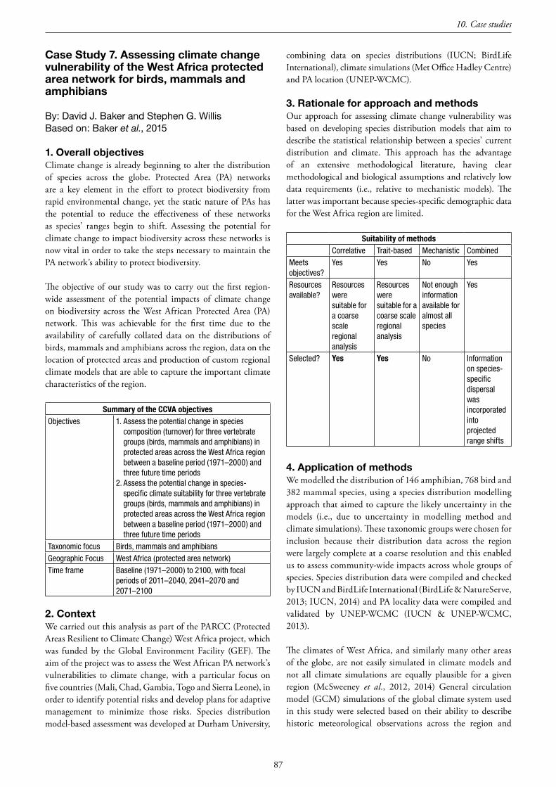
87

CaseStudy7.AssessingclimatechangevulnerabilityoftheWestAfricaprotectedareanetworkforbirds,mammalsandamphibians

By: David J. Baker and Stephen G. WillisBased on: Baker et al., 2015

1.OverallobjectivesClimate change is already beginning to alter the distribution of species across the globe. Protected Area (PA) networks are a key element in the effort to protect biodiversity from rapid environmental change, yet the static nature of PAs has the potential to reduce the effectiveness of these networks as species’ ranges begin to shift. Assessing the potential for climate change to impact biodiversity across these networks is now vital in order to take the steps necessary to maintain the PA network’s ability to protect biodiversity.

The objective of our study was to carry out the first region-wide assessment of the potential impacts of climate change on biodiversity across the West African Protected Area (PA) network. This was achievable for the first time due to the availability of carefully collated data on the distributions of birds, mammals and amphibians across the region, data on the location of protected areas and production of custom regional climate models that are able to capture the important climate characteristics of the region.

Summary of the CCVA objectivesObjectives 1. Assessthepotentialchangeinspecies

composition(turnover)forthreevertebrategroups(birds,mammalsandamphibians)inprotectedareasacrosstheWestAfricaregionbetweenabaselineperiod(1971–2000)andthreefuturetimeperiods

2. Assessthepotentialchangeinspecies-specificclimatesuitabilityforthreevertebrategroups(birds,mammalsandamphibians)inprotectedareasacrosstheWestAfricaregionbetweenabaselineperiod(1971–2000)andthreefuturetimeperiods

Taxonomicfocus Birds,mammalsandamphibiansGeographicFocus WestAfrica(protectedareanetwork)Timeframe Baseline(1971–2000)to2100,withfocal

periodsof2011–2040,2041–2070and2071–2100

2.ContextWe carried out this analysis as part of the PARCC (Protected Areas Resilient to Climate Change) West Africa project, which was funded by the Global Environment Facility (GEF). The aim of the project was to assess the West African PA network’s vulnerabilities to climate change, with a particular focus on five countries (Mali, Chad, Gambia, Togo and Sierra Leone), in order to identify potential risks and develop plans for adaptive management to minimize those risks. Species distribution model-based assessment was developed at Durham University,

combining data on species distributions (IUCN; BirdLife International), climate simulations (Met Office Hadley Centre) and PA location (UNEP-WCMC).

3.RationaleforapproachandmethodsOur approach for assessing climate change vulnerability was based on developing species distribution models that aim to describe the statistical relationship between a species’ current distribution and climate. This approach has the advantage of an extensive methodological literature, having clear methodological and biological assumptions and relatively low data requirements (i.e., relative to mechanistic models). The latter was important because species-specific demographic data for the West Africa region are limited.

Suitability of methodsCorrelative Trait-based Mechanistic Combined

Meetsobjectives?

Yes Yes No Yes

Resourcesavailable?

Resourcesweresuitableforacoarsescaleregionalanalysis

Resourcesweresuitableforacoarsescaleregionalanalysis

Notenoughinformationavailableforalmostallspecies

Yes

Selected? Yes Yes No Informationonspecies-specificdispersalwasincorporatedintoprojectedrangeshifts

4.ApplicationofmethodsWe modelled the distribution of 146 amphibian, 768 bird and 382 mammal species, using a species distribution modelling approach that aimed to capture the likely uncertainty in the models (i.e., due to uncertainty in modelling method and climate simulations). These taxonomic groups were chosen for inclusion because their distribution data across the region were largely complete at a coarse resolution and this enabled us to assess community-wide impacts across whole groups of species. Species distribution data were compiled and checked by IUCN and BirdLife International (BirdLife & NatureServe, 2013; IUCN, 2014) and PA locality data were compiled and validated by UNEP-WCMC (IUCN & UNEP-WCMC, 2013).

The climates of West Africa, and similarly many other areas of the globe, are not easily simulated in climate models and not all climate simulations are equally plausible for a given region (McSweeney et al., 2012, 2014) General circulation model (GCM) simulations of the global climate system used in this study were selected based on their ability to describe historic meteorological observations across the region and

10. Case studies

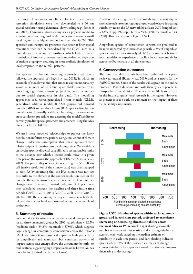
88

IUCN SSC Guidelines for Assessing Species’ Vulnerability to Climate Change

Decreasing Increasing

Mammals

Birds

Amphibians

Mammals

Birds

Birds

Mammals

Amphibians

Amphibians

2100

2070

2040

Number of species projected to experience increasing/decreasing climate suitability

700 500 300 100 100 300 500 700

Figure CS7.1. Number of species within each taxonomic group, and in each time period, projected to experience increasing or decreasing climate suitability across the West African PA network. Light shading shows the number of species with increasing or decreasing suitability across the network based on the median estimate of suitability in each time period, and dark shading indicates species where 95% of the projected estimates of change in climate suitability for a species showed directional consensus (increasing or decreasing).

the range of responses to climate forcing. These coarse resolution simulations were then downscaled to a 50  km spatial resolution using dynamical downscaling (e.g., Jones et al., 2004). Dynamical downscaling uses a physical model to simulate local and regional scale interactions across a small focal region at a higher resolution than the GCM. This approach can incorporate processes that occur at finer spatial resolutions than can be considered by the GCM, such as a more detailed depiction of coastlines, which leads to better simulation of land-sea processes, and a more detailed depiction of surface orography, resulting in more realistic simulation of local temperature and rainfall patterns.

The species distribution modelling approach used closely followed the approach of (Bagchi et al., 2013), in which an ensemble of models was built that aimed to capture uncertainty across a number of different quantifiable sources (e.g., modelling algorithm, climate projections, and uncertainty due to spatial dependency in the data). The modelling approaches used were: generalized linear models (GLM), generalized additive models (GAM), generalized boosted models (GBM) and random forests (RF). Species distribution models were internally validated by using a leave-one-out cross-validation procedure and assessing the model’s ability to correctly predict species presences and absences using the Area Under the Curve (AUC).

We used these modelled relationships to project the likely distribution in future time periods using simulations of climate change under the assumption that these species-climate relationships will remain constant through time. We used data on species-specific dispersal capabilities to set reasonable limits to the distance over which a species could move in a given time period (following the approach of (Barbet-Massin et al., 2012). The probability of a species occurring in a 50 x 50 km cell (native resolution of the climate data) was then mapped to each PA by assuming that the PA’s climate was not too dissimilar to the climate at the coarser resolution used in the models. The species turnover, which is a metric of community change over time and a useful indicator of impact, was then calculated between the baseline and three future time periods (‘2040’ = 2011–2040; ‘2070’ = 2041–2070; ‘2100’ = 2071–2100). The uncertainty in projected impacts at both the PA and the species level was assessed across the ensemble of projections.

5.SummaryofresultsSubstantial species turnover across the network was projected for all three taxonomic groups by 2100 (amphibians = 42.5% (median); birds = 35.2%; mammals = 37.9%), which suggests large change in community composition across the region’s PAs. Uncertainty in our projected impacts is high, particularly for amphibians and mammals, but consistent patterns of impacts across taxa emerge above the uncertainty by early- to mid-century, suggesting high impacts across the Lower Guinea forest biome (centred on the Ivory Coast).

Based on the change in climate suitability, the majority of species in each taxonomic group are projected to have decreasing suitability across the PA network by at least 2070 [amphibians = 63% of spp. (92 spp.); birds = 55% (419); mammals = 63% (239)]. This can be seen in Figure CS7.1.

Amphibian species of conservation concern are predicted to be most impacted by climate change with >75% of amphibian species projected as ‘extremely likely’ (i.e., agreement between most models) to experience a decline in climate suitability across the PA network in all time periods.

6.ConservationoutcomesThe results of this analysis have been published in a peer-reviewed journal (Baker et al., 2015) and as a report for the PARCC project. Some of the results will appear on the online Protected Planet database and will thereby alert people to PA-specific vulnerabilities. These results are likely to be used in the future to guide focal research in the region. However, at present it is too early to comment on the impact of these vulnerability assessments.

89

7.RoomforimprovementThe major difficulties in conducting a large-scale climate change vulnerability assessment result from data limitations and the mismatch between the spatial resolution of the data and the scale at which individual organisms respond to the environment. Coarse resolution assessments of climate change vulnerabilities should now be used to inform field-based studies on the most vulnerable species and the locations likely to experience the greatest environmental change. This must include basic population monitoring across divergent taxonomic groups (plants, invertebrates, mammals, birds) and detailed demographic monitoring of focal species, specifically collecting information on abundance, productivity and survival. This information will be vital for understanding the mechanisms linking demographic changes to environmental changes, and will help inform conservation decisions in the future.

An important component of this project was the close collaboration with the climate scientists providing the regional climate simulation data. Our approach for selection of the GCMs and downscaling these data to finer-scale projections provides some degree of confidence that this study is based on climate simulations that are regionally plausible (Buontempo et al., 2015). However, the considerable technical overheads involved in producing these climate simulations are likely to be prohibitive in many cases, and a consequence is that our impact assessment explores only a single ‘middle-of-the-road’ emissions pathway, which might be overly conservative. Our study does, however, incorporate uncertainty in historic climate data (although here simulated), which has been shown to be important for ecological impact assessments (Baker et al., 2016). Overall, there is much scope to improve the use of climate data in ecological impact assessments, but we hope that the approach taken here provides some ideas for good practice.

8.ReferencesBagchi R., Crosby M., Huntley B., Hole D.G., Butchart S.H.M.,

Collingham Y., Kalra M., Rajkumar J., Rahmani A., Pandey M., Gurung H., Trai L.T., Van Quang N., & Willis S.G. (2013) Evaluating the effectiveness of conservation site networks under climate change: accounting for uncertainty. Global Change Biology, 19:1236–48.

Baker D.J., Hartley A.J., Burgess N.D., Butchart S.H.M., Carr J.A., Smith R.J., Belle E., & Willis S.G. (2015) Assessing climate change impacts for vertebrate fauna across the West African protected area network using regionally appropriate climate projections. Diversity and Distributions, 21:991–1003.

Baker D.J., Hartley A.J., Butchart S., & Willis S.G. (2016) Choice of baseline climate data impacts projected species’ responses to climate change. Global Change Biology, 22:2392–2404.

Barbet-Massin M., Thuiller W., & Jiguet F. (2012) The fate of European breeding birds under climate, land-use and dispersal scenarios. Global Change Biology, 18:881–890.

BirdLife & NatureServe (2013) Bird species distribution maps of the world. Version 3.0.

Buontempo C., Mathison C., Jones R., Williams K., Wang, C., & McSweeney C. (2015) An ensemble climate projection for Africa. Climate Dynamics, 44:2097–2118.

IUCN (2014) The IUCN Red List of Threatened Species. Version 2014.2.

IUCN & UNEP-WCMC (2013) The World Database on Protected Areas (WDPA) [December Release].

Jones R., Noguer M., Hassell D., Hudson D., Wilson S., Jenkins G., & Mitchell J. (2004) Generating high resolution climate change scenarios using PRECIS. Met Office Hadley Centre, Exeter, UK.

McSweeney C.F., Jones R., & Booth B. (2012) Selecting Ensemble Members to Provide Regional Climate Change Information. Journal of Climate, 25:7100–7121.

McSweeney C.F., Jones R., Lee R., & Rowell D. (2014) Selecting CMIP5 GCMs for downscaling over multiple regions. Climate Dynamics, 44:3237–3260.

CaseStudy8.Correlative-mechanisticCCVAoftheIberianLynx

By: Resit AkcakayaBased on: Fordham et al., 2013

1.OverallobjectivesThis case study focuses on assessing climate change vulnerability of the Iberian Lynx (Lynx pardinus), as well as the effectiveness of conservation plans for its recovery. The Iberian Lynx is at risk of extinction due to the combined and interacting effects of climate change and habitat loss affecting both the lynx and its primary prey species, the European Rabbit (Oryctolagus cuniculus), as well as the effects of two diseases on the prey species (Fordham et al., 2013).

Summary of the CCVA objectivesObjectives 1.HowvulnerableistheIberianLynxtoextinction

underdifferentclimatechangescenarios?2.Howeffectivearethecurrentconservation

measuresplannedforthespecies?3.Howeffectivewouldanewconservationplanbe

thattakesclimatechangeintoaccount?Taxonomicfocus

IberianLynxanditspreyspecies,theEuropeanRabbit

Geographicfocus

TheIberianPeninsula(totalcurrentandfutureexpectedrangeofthelynx)

Timeframe Frompresent(2013)totheendofthecentury(2090)

Going beyond this particular species, a broader objective of the study was to provide a framework for a next-generation model which simultaneously incorporates demography, dispersal, and biotic interactions (predation and disease) into estimation of extinction risk and evaluation of conservation plans under projected climate change (Kissling 2013).

2.ContextThe Iberian Lynx (Lynx pardinus) is one of world’s most threatened mammal species, and is considered to be on the brink of extinction. The population size and the range of the Iberian lynx have declined sharply since the 1950s. More than 80% of the diet of the Iberian Lynx consists of European Rabbit (Oryctolagus cuniculus), whose abundance has sharply declined because of the myxomatosis virus in the 1950s, rabbit haemorrhagic disease in recent decades, as well as over-hunting and the loss and fragmentation of its habitat. In addition,

10. Case studies

90

IUCN SSC Guidelines for Assessing Species’ Vulnerability to Climate Change

human-caused mortality of Iberian Lynx due to poisoning, poaching and road kills have contributed to the reduction of the lynx population.

To prevent the extinction of Iberian Lynx, captive breeding programmes have been initiated to facilitate the species’ reintroduction into suitable areas within their historical range, in parallel with management aimed at increasing the carrying capacity of reintroduction sites. Climate change could further threaten the survival of the species, but recovery plans for the species have not incorporated the projected changes in climate.

3.RationaleforapproachandmethodsThe approach used in this case study is based on the idea that the conservation status and recovery of species are determined both by their habitat and their demographic traits or characteristics. As a result, approaches that rely only on projected habitat cannot adequately assess species’ vulnerability, nor evaluate conservation options for their recovery. Especially for assessments of species where there is a strong biotic interaction with another species (such as a predator dependent on a single prey species), biotic interactions must be explicitly incorporated.

The Iberian Lynx is affected by multiple threats, and is also subject to predator-prey dynamics where the lynx almost exclusively relies on the rabbit, which in turn is impacted by diseases. Assessing the species therefore required a novel approach that combined demography, spatial dynamics, and biotic interactions. Fordham et al. (2013) used ecological niche models coupled to metapopulation simulations with source-sink dynamics, to directly investigate the combined effects of climate change, prey availability and management intervention on the persistence of the Iberian Lynx. This approach is novel in that it explicitly models dynamic bi-trophic species interactions in a climate change setting.

Suitability of methodsCorrelative Trait-based Mechanistic Combined

Meets objectives?

Inpart No Inpart Yes

Resources available?

Yes Yes Yes Yes

Selected? No No No Yes

4.ApplicationofmethodsFordham et al. (2013) collated information on the following aspects of the lynx-rabbit system:• Geo-referenced occurrence records of the Iberian Lynx and

European rabbit.• Data on annual rainfall and mean temperature of the hottest

and coolest months (July and January, respectively). Based on previous studies, these climatic variables were identified as being likely to have the largest potential climate influence on Iberian Lynx and European Rabbit abundance.

• Annual time series of these climate change variables, generated according to two emissions scenarios.

• Land cover data (map of land cover types).• Protected Area map.• Time series data for European rabbit, extracted from the

Global Population Dynamics Database.• Information on the demography of the Iberian Lynx

(including age-specific survival and fecundity, and density dependence), and European rabbit (including disease dynamics), based on previous studies.

Using these data, Fordham et al. (2013) developed ecological niche models and demographic (metapopulation) models for both species. For each species, the ecological niche model determined the carrying capacities and spatial arrangement of habitat patches, forming the spatial basis of the demographic model, which was dynamic in order to simulate temporal changes in the species’ habitat. This linkage between the niche and demographic models followed methods that have been applied in previous cases (Akçakaya et al., 2004, 2005; Keith et al., 2008; Fordham et al., 2012). What was novel about this study was the linkage of the models for the two species to simulate biotic interactions. Briefly, the results of the rabbit model were used as input for the lynx model, such that rabbit abundance at each time step of the simulation was one of the factors (in addition to climate and land cover) that contributed to the lynx population dynamics.

In addition to running the models to estimate the extinction risk of the lynx without any conservation measures, the lynx model was modified to test the effectiveness of translocation of lynxes to suitable areas as a conservation measure. Two conservation measures were tested: the current conservation plan and a plan optimized under climate change.

5.SummaryofresultsThe results showed that anticipated climate change will rapidly and severely decrease lynx abundance and is likely to lead to the species’ extinction in the wild within 50 years, even with strong global efforts to mitigate greenhouse gas emissions. However, the results also showed that a carefully planned reintroduction programme, accounting for the effects of climate change, prey abundance and habitat connectivity, could prevent the extinction of the lynx and result in a robust recovery. In contrast, the results showed that the current conservation plan, which does not incorporate the effects of climate change, is not likely to lead to the recovery of the Iberian lynx, and may not even prevent its extinction.

6.ConservationoutcomesAs more species are impacted by climate change and habitat loss, conservation translocations are likely to be more commonly used. An important step in planning conservation translocation is to quantify the effectiveness of alternative translocation plans, which may differ in terms of the location of source and target populations, the number, sex, and age

91

of individuals to be translocated, and the frequency and timing of translocations. This can be done by simulating the dynamics of the focal species with models in which potential source and target populations are modelled as subpopulations of a metapopulation (e.g., Kuemmerle et al., 2011). This study demonstrated the use of models in quantifying the effects of translocations on species and, for the first time, the importance of incorporating prey availability, climate change and their interaction in models to design conservation plans to prevent species extinctions.

7.ReferencesAkçakaya; H. R., J. Franklin, A. D. Syphard, and J. R. Stephenson. 2005.

Viability of bell’s sage sparrow (amphispiza belli ssp. belli ): altered fire regimes 15:521–531.

Akçakaya; H. R., V. C. Radeloff, D. J. Mladenoff, and H. S. He. 2004. Integrating Landscape and Metapopulation Modeling Approaches : Viability of the Sharp-Tailed Grouse in a Dynamic Landscape. Conservation Biology 18:526–537.

Fordham; D. A., H. R. Akçakaya, B. W. Brook, A. Rodríguez, P. C. Alves, E. Civantos, M. Triviño, M. J. Watts, and M. B. Araújo. 2013. Adapted conservation measures are required to save the Iberian lynx in a changing climate. Nature Climate Change 3:899–903.

Fordham; D. A., H. Resit Akçakaya, M. B. Araújo, J. Elith, D. A. Keith, R. Pearson, T. D. Auld, C. Mellin, J. W. Morgan, T. J. Regan, M. Tozer, M. J. Watts, M. White, B. A. Wintle, C. Yates, and B. W. Brook. 2012. Plant extinction risk under climate change: Are forecast range shifts alone a good indicator of species vulnerability to global warming? Global Change Biology 18:1357–1371.

Keith; D. A., H. R. Akçakaya, W. Thuiller, G. F. Midgley, R. G. Pearson, S. J. Phillips, H. M. Regan, M. B. Araújo, and T. G. Rebelo. 2008. Predicting extinction risks under climate change: coupling stochastic population models with dynamic bioclimatic habitat models. Biology Letters 4:560–563.

Kissling; W. D. 2013. Estimating extinction risk under future climate change: next-generation modeling simultaneously incorporates demography, dispersal, and biotic interactions. Frontiers of Biogeography 5:3–6.

Kuemmerle; T., K. Perzanowski, H. R. Akcakaya, F. Beaudry, T. R. Van Deelen, I. Parnikoza, P. Khoyetskyy, D. M. Waller, and V. C. Radeloff. 2011. Cost‐effectiveness of strategies to establish a European bison metapopulation in the Carpathians. Journal of Applied Ecology 48:317–329.

CaseStudy9.MatchingspeciestraitstocorrelativemodelprojectionsinacombinedCCVAapproach

By: Raquel A. GarciaBased on: Garcia et al., 2012

1.OverallobjectivesAssessing the vulnerability of species to climate change requires an understanding of species’ exposure to extrinsic threats, and of their intrinsic sensitivity or adaptive capacity to respond to such threats. Whereas trait-based approaches can combine the components of exposure and sensitivity/ adaptive capacity to derive vulnerability scores, the measures of exposure used are often simplistic and spatially confined to the present range of the species. By relying on correlative models to assess exposure, the losses, gains and fragmentation of areas of suitable climate can be mapped to gain a better understanding of the different threats (and opportunities) that species may face. Each threat can then be compared to intrinsic traits that might mediate the response of species to that particular threat. Specific traits are likely to mediate species’ responses to different threats (Isaac and Cowlishaw 2004, Murray et al., 2011), but this specificity has hitherto not been sufficiently addressed in CCVAs. Here we present a combined CCVA approach that borrows strength from both correlative models and traits and yields spatially explicit outputs.

The productivity of Central Africa’s Lake Tanganyika is predicted to decline. The extreme depth of the lake causes convection currents that bring nutrient-rich deeper waters to the surface, making the lake highly productive. However, climate change driven warming of surface water is predicted to decrease the extent of mixing. Fishermen in the Tanzanian village of Kala report reductions in their fish catch over the last decade; productivity declines are also likely to affect lake ecosystems and species. © Wendy B. Foden

10. Case studies

91

92

IUCN SSC Guidelines for Assessing Species’ Vulnerability to Climate Change

We use published results of correlative models for 195 species of sub-Saharan African amphibians (Garcia et al., 2012), and quantify the degree of loss, gain and fragmentation of climatically suitable areas for each. Based on previously published empirical and theoretical work, we then identify potential ‘response-mediating traits’ for each projected change, and gather those for which there are data available for our species. By spatially overlaying areas of projected extrinsic changes and areas of high intrinsic vulnerability, we map geographical areas where species are both exposed and vulnerable to climate change.

Summary of the CCVA objectivesObjectives 1. Todescribeprojectedextrinsicthreatsand

opportunitiesfromclimatechangegivenbycorrelativemodels:losses,gainsandfragmentationofsuitableclimatespaceforspecies.

2. Toselecttraitsthatmightmediatespecies’responsestoeachofthosethreatsandopportunities.

3. Toexaminethespatialoverlapbetweenthetwo,soastoidentifyareaswherespeciesmightbebothexposedtoextrinsicthreatsandintrinsicallyvulnerabletothem.

Taxonomicfocus AmphibiansGeographicfocus Sub-SaharanAfricaTimeframe From1961–90to2050

2.ContextWe focused on sub-Saharan African amphibians for three reasons. First, these species are expected to be highly vulnerable to climate change. Worldwide, amphibian populations are declining due to a multitude of threats that include habitat destruction, climate change and the fungal disease chytridiomycosis (Blaustein and Kiesecker 2002, Hof et al., 2011, Li et al., 2013). Climate change, often in tandem with land-use change, is expected to affect large areas of tropical Africa in the future (Hof et al., 2011, Foden et al., 2013). Second, we take advantage of available correlative model results (Garcia et al., 2012) and trait data (Foden et al., 2013). Third, a case study focused on sub-Saharan African amphibians illustrates the application of our framework when traits in the strict sense (Violle et al., 2007) are largely unavailable, a situation that is common for many taxonomic groups (González-Suárez et al., 2012). The work brought together researchers involved in previous correlative model work (Raquel A. Garcia, Miguel B. Araújo, Mar Cabeza, Carsten Rahbek and Neil D. Burgess) and trait-based work (Wendy B. Foden and Alexander Gutsche).

3.RationaleforapproachandmethodsOur aim was to identify geographical areas where species are potentially exposed to threats from climate change through sensitivity or a lack of the adaptive capacity to respond to them. We also wanted to understand where climate change presents opportunities for species to expand their ranges.

While mechanistic models would be the most suitable CCVA method to address this question, we lacked the physiological data required. Trait-based methods would only partly address the question, without determining the opportunities for new climatically suitable areas and the threat of fragmentation of climatically suitable areas. Because we had results available from correlative models as well as trait data, we selected a combination of correlative and trait-based methods.

Suitability of methodsCorrelative Trait-

basedMechanistic Combined

Meetsobjectives? No Yes Yes YesResourcesavailable? Yes Yes No YesSelected? No No No Yes

For consideration of projected losses, increased fragmentation and gains of climate space, we selected potential response-mediating traits and examined the spatial overlap with vulnerability due to traits that were deemed relevant in each case. We examined the overlap for all species, and individually for groups of species with different combinations of threats and opportunities.

4.ApplicationofmethodsWe applied the framework to 195 sub-Saharan African amphibians with both available bioclimatic envelope model projections for the mid-21st century (Garcia et al., 2012) and trait data (Foden et al., 2013). Excluded were 500 narrow-ranging species that mainly occur in montane areas. Correlative model results and trait data (provided in spreadsheets) were processed and mapped in R (R Development Core Team 2010).

First, to characterize climate change-induced threats and opportunities for each species, we compared the projections of baseline and future climatic suitability to compute losses, fragmentation and gains of climatic suitability, and calculated the distances to new areas gained. We obtained maps of changes for each species, and compiled composite maps for all species by summing individual maps.

Second, based on theoretical and empirical studies, we selected potential ‘response-mediating traits’ for each threat. Among these, we selected the traits (or proxies for traits) for which we had available data. For each trait, we assigned species “high”, lower” or “unknown” sensitivity/ adaptive capacity scores, based on pre-selected thresholds (Foden et al., 2013). Third, we mapped each extrinsic threat and overlaid it with the maps for the classification of relevant traits for that threat. For each combination of extrinsic threat and response-mediating trait (e.g., projected gains in climatic suitability and dispersal ability), we obtained gridded outputs for the number of species exposed to a threat and considered sensitive or having low adaptive capacity to respond to that threat versus the number of species exposed to a threat but considered less sensitive or having high adaptive capacity to respond to that threat.

93

5.SummaryofresultsThe gridded outputs were mapped to determine areas where exposure and high sensitivity and/or low adaptive capacity overlapped for many species. In the Congo Basin and arid Southern Africa, projected losses for wide-ranging amphibians were compounded by sensitivity to climatic variation, and expected gains were precluded by poor dispersal ability. The spatial overlap between exposure and vulnerability was more pronounced for species projected to have their climate space contracting in situ or shifting to distant geographical areas. Our results excluded the potential exposure of range-restricted species to shrinking areas of suitable climate in the African tropical mountains.

6.ConservationoutcomesThe work was published in the Journal of Biogeography (Garcia et al., 2014). We illustrate the application of a framework combining spatial projections of climate change exposure with traits that are likely to mediate species’ responses. Although the proposed framework carries several assumptions that require further scrutiny, its application adds a degree of realism to familiar CCVAs based on correlative models that consider all species to be equally affected by climate change-induced threats and opportunities.

7.RoomforimprovementThe trait data used here are mainly ecological characteristics of species or their ranges rather than traits in a strict sense (Violle et al., 2007), and thus do not strictly summarize traits, but rather the interaction between traits and the environment. High quality trait data are often not easily accessible, but, when possible, data should be used that rely on direct measurement of traits. For example, measurement of tolerance to climatic variation, here inferred with statistical approaches relating current ranges of species to climate variables, should instead rely on an experimental approach applied to estimating the safety thermal limits (Arribas et al., 2012). Likewise, estimates of species’ dispersal abilities derived from empirical data on organism movement (e.g., Gamble et al., 2007), phylogenetic distances (Arribas et al., 2012), or morphological or life-history traits (Whitmee et al., 2012, Baselga et al., 2012) would more reliably predict the ability of species to track suitable climates than estimates based on known geographical ranges of species as applied here. By the same token, the thresholds for classification of species’ sensitivity or adaptive capacity based on selected traits should, when possible, be empirically based.

Due to data limitations (with respect to traits, but mainly to available correlative models), the analysis excludes most threatened amphibians, particularly those from the Cameroon highlands and Eastern Afromontane centres of diversity. Phylogenetic inference methods exist that could circumvent the bias in the trait data (Nakagawa and Freckleton 2008, Buckley and Kingsolver 2012), but, for the bulk of the species excluded here, new approaches that overcome limitations of

correlative models are needed to assess the vulnerability of range-restricted species to climate change.

8.ReferencesArribas; P., P. Abellán, J. Velasco, D. T. Bilton, A. Millán, and D.

Sánchez-Fernández. 2012. Evaluating drivers of vulnerability to climate change: a guide for insect conservation strategies. Global Change Biology 18:2135–2146.

Baselga; A., J. M. Lobo, J.-C. Svenning, P. Aragón, and M. B. Araújo. 2012. Dispersal ability modulates the strength of the latitudinal richness gradient in European beetles. Global Ecology and Biogeography 21:1106–1113.

Blaustein; A. R., and J. M. Kiesecker. 2002. Complexity in conservation: lessons from the global decline of amphibian populations. Ecology Letters 5:597–608.

Buckley; L. B., and J. G. Kingsolver. 2012. Functional and phylogenetic approaches to forecasting species’ responses to climate change. Annual Review of Ecology, Evolution, and Systematics 43:205–226.

Foden; W. B., S. H. M. Butchart, S. N. Stuart, J.-C. Vié, H. R. Akçakaya, A. Angulo, L. M. DeVantier, A. Gutsche, E. Turak, L. Cao, S. D. Donner, V. Katariya, R. Bernard, R. A. Holland, A. F. Hughes, S. E. O’Hanlon, S. T. Garnett, Ç. H. Şekercioğlu, and G. M. Mace. 2013. Identifying the World’s Most Climate Change Vulnerable Species: A Systematic Trait-Based Assessment of all Birds, Amphibians and Corals. PLoS One 8:e65427.

Gamble; L. R., K. McGarigal, and B. W. Compton. 2007. Fidelity and dispersal in the pond-breeding amphibian, Ambystoma opacum: Implications for spatio-temporal population dynamics and conservation. Biological Conservation 139:247–257.

Garcia; R. A., M. B. Araújo, N. D. Burgess, W. B. Foden, A. Gutsche, C. Rahbek, and M. Cabeza. 2014. Matching species traits to projected threats and opportunities from climate change. Journal of Biogeography 41:724–735.

Garcia; R. A., N. D. Burgess, M. Cabeza, C. Rahbek, and M. B. Araújo. 2012. Exploring consensus in 21st century projections of climatically suitable areas for African vertebrates. Global Change Biology 18:1253–1269.

González-Suárez; M., P. M. Lucas, and E. Revilla. 2012. Biases in comparative analyses of extinction risk: mind the gap. Journal of Animal Ecology 81:1211–1222.

Hof; C., M. B. Araújo, W. Jetz, and C. Rahbek. 2011. Additive threats from pathogens, climate and land-use change for global amphibian diversity. Nature 480:516–519.

Isaac; N. J. B., and G. Cowlishaw. 2004. How species respond to multiple extinction threats. Proceedings. Biological sciences / The Royal Society 271:1135–41.

Li; Y., J. M. Cohen, and J. R. Rohr. 2013. Review and synthesis of the effects of climate change on amphibians. Integrative Zoology 8:145–161.

Murray; K. A., D. Rosauer, H. McCallum, and L. F. Skerratt. 2011. Integrating species traits with extrinsic threats: closing the gap between predicting and preventing species declines. Proceedings of the Royal Society of London Series B: Biological Sciences 278:1515–23.

Nakagawa; S., and R. P. Freckleton. 2008. Missing inaction: the dangers of ignoring missing data. Trends in Ecology & Evolution 23:592–596.

R Development Core Team. 2010. R: A language and environment for statistical computing. R Foundation for Statistical Computing, Vienna, Austria.

Violle; C., M.-L. Navas, D. Vile, E. Kazakou, C. Fortunel, I. Hummel, and E. Garnier. 2007. Let the concept of trait be functional! Oikos 116:882–892.

Whitmee; S., C. D. L. Orme, and M. Humphries. 2012. Predicting dispersal distance in mammals: a trait-based approach. The Journal of Animal Ecology 82:211–221.

10. Case studies

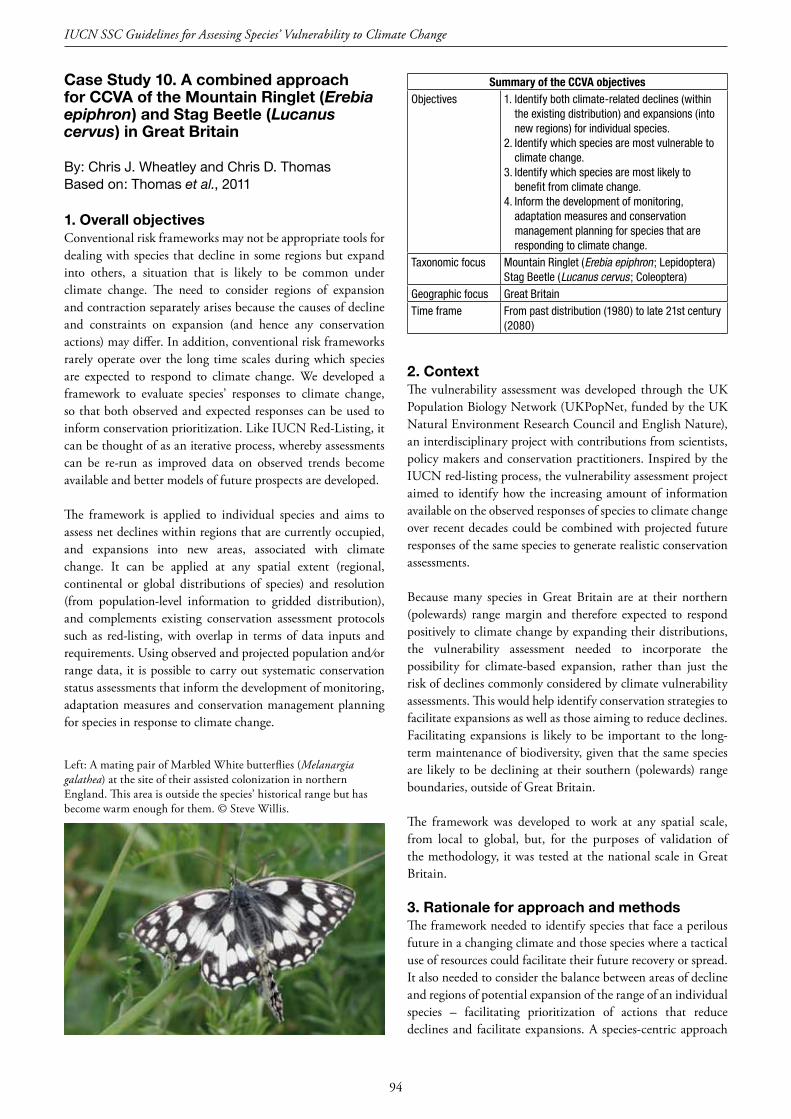
94

IUCN SSC Guidelines for Assessing Species’ Vulnerability to Climate Change

CaseStudy10.AcombinedapproachforCCVAoftheMountainRinglet(Erebia epiphron)andStagBeetle(Lucanus cervus)inGreatBritain

By: Chris J. Wheatley and Chris D. ThomasBased on: Thomas et al., 2011

1.OverallobjectivesConventional risk frameworks may not be appropriate tools for dealing with species that decline in some regions but expand into others, a situation that is likely to be common under climate change. The need to consider regions of expansion and contraction separately arises because the causes of decline and constraints on expansion (and hence any conservation actions) may differ. In addition, conventional risk frameworks rarely operate over the long time scales during which species are expected to respond to climate change. We developed a framework to evaluate species’ responses to climate change, so that both observed and expected responses can be used to inform conservation prioritization. Like IUCN Red-Listing, it can be thought of as an iterative process, whereby assessments can be re-run as improved data on observed trends become available and better models of future prospects are developed.

The framework is applied to individual species and aims to assess net declines within regions that are currently occupied, and expansions into new areas, associated with climate change. It can be applied at any spatial extent (regional, continental or global distributions of species) and resolution (from population-level information to gridded distribution), and complements existing conservation assessment protocols such as red-listing, with overlap in terms of data inputs and requirements. Using observed and projected population and ⁄or range data, it is possible to carry out systematic conservation status assessments that inform the development of monitoring, adaptation measures and conservation management planning for species in response to climate change.

Summary of the CCVA objectivesObjectives 1. Identifybothclimate-relateddeclines(within

theexistingdistribution)andexpansions(intonewregions)forindividualspecies.

2. Identifywhichspeciesaremostvulnerabletoclimatechange.

3. Identifywhichspeciesaremostlikelytobenefitfromclimatechange.

4. Informthedevelopmentofmonitoring,adaptationmeasuresandconservationmanagementplanningforspeciesthatarerespondingtoclimatechange.

Taxonomicfocus MountainRinglet(Erebia epiphron ;Lepidoptera)StagBeetle(Lucanus cervus ;Coleoptera)

Geographicfocus GreatBritainTimeframe Frompastdistribution(1980)tolate21stcentury

(2080)

2.ContextThe vulnerability assessment was developed through the UK Population Biology Network (UKPopNet, funded by the UK Natural Environment Research Council and English Nature), an interdisciplinary project with contributions from scientists, policy makers and conservation practitioners. Inspired by the IUCN red-listing process, the vulnerability assessment project aimed to identify how the increasing amount of information available on the observed responses of species to climate change over recent decades could be combined with projected future responses of the same species to generate realistic conservation assessments.

Because many species in Great Britain are at their northern (polewards) range margin and therefore expected to respond positively to climate change by expanding their distributions, the vulnerability assessment needed to incorporate the possibility for climate-based expansion, rather than just the risk of declines commonly considered by climate vulnerability assessments. This would help identify conservation strategies to facilitate expansions as well as those aiming to reduce declines. Facilitating expansions is likely to be important to the long-term maintenance of biodiversity, given that the same species are likely to be declining at their southern (polewards) range boundaries, outside of Great Britain.

The framework was developed to work at any spatial scale, from local to global, but, for the purposes of validation of the methodology, it was tested at the national scale in Great Britain.

3.RationaleforapproachandmethodsThe framework needed to identify species that face a perilous future in a changing climate and those species where a tactical use of resources could facilitate their future recovery or spread. It also needed to consider the balance between areas of decline and regions of potential expansion of the range of an individual species – facilitating prioritization of actions that reduce declines and facilitate expansions. A species-centric approach

Left: A mating pair of Marbled White butterflies (Melanargia galathea) at the site of their assisted colonization in northern England. This area is outside the species’ historical range but has become warm enough for them. © Steve Willis.

95

was also required as it is species, and not entire communities, that shift their distributions in response to climate change (although common conservation measures may meet the needs of multiple individual species). The framework aims to provide a risk assessment for each species, with the development of any conservation actions flowing from the assessment, rather than being incorporated within the framework itself.

The approach of the Thomas et al. (2011) framework (a)  incorporates information on both observed and projected trends (flexibly using population and/or distribution data) to maximize the information that is included; (b) treats habitat and trait data (e.g., dispersal) as constraints to evaluate the likelihood that climate-only projections will be realized or exacerbated; (c) considers uncertainty in the assessment; and (d) provides assessments over time scales that are relevant to climate change and conservation, given that we are already committed to ~100 years of climate change (even with optimistic climate mitigation measures). Trait data are considered to be modifiers of the expected response rather than primary drivers of vulnerability, given that relationships between traits and climate change responses are unlikely to be strong across the full range of taxa (e.g., plants, invertebrates, vertebrates) that will need to be assessed.

Data for a correlative approach to the assessment were available for all species of interest, so resource requirements were not a limiting factor. Previous studies of the species within the assessment area provided the necessary trait data. These population and trait approaches could be combined without the potentially high resource cost in terms of time and financial need that may have been the case for less well studied taxa. Flexibility of the approach (e.g., just using modelled distribution data) makes assessments possible even for regions and taxa where information is limited, but inevitably such assessments will be assigned lower levels of confidence.

Suitability of methodsCorrelative Trait-based Mechanistic Combined

Meetsobjectives?

Inpart Inpart Yes Yes

Resourcesavailable?

Yes Yes Dataavailabilityinsufficientforsomespecies

Yes

Selected? No No No Yes

Data inputs required to run the assessment are little different from those required for other conservation assessments (e.g. red-listing, species action plans), which allowed the framework to be run in a reasonable time frame while taking advantage of existing data.

The framework gives equal focus to benefits of climate change, assigning levels of benefit in the same way as is done for risk. Many other climate vulnerability assessments simply combine all species with any opportunities under climate change into a

single low risk category, but the degree to which species may benefit is potentially as interesting as how likely they are to decline. The framework also attempts to incorporate the level of certainty in the input data and conclusions of the assessment, allowing for anyone interpreting the results of the assessment to not only consider the potential risk or benefit faced by a species, but also have an idea of the level of support for the conclusions of any assessment.

4.ApplicationofmethodsThe Mountain Ringlet Butterfly (Erebia epiphron) and Stag Beetle (Lucanus cervus) were selected as case study species for the assessment due to their opposite range margins in the assessment area (northern vs. southern, respectively) and to test how applicable the assessment was across different taxonomic groups.

The framework method combines a decline score (based on observed and projected declines) with an increase score (observed increase and projected increases) to produce on overall assessment of potential risk for a species. Each stage of the assessment is also scored based on the level of confidence in the input data or model; and this score is used to weight the assessment towards information that is most certain. The overall score is converted to one of six risk categories ranging from high benefit to high risk.

Future distributions of the target species had already been modelled and historical distribution/population data within Great Britain were readily available. Historic distribution and population changes for the mountain ringlet were obtained from published sources with data back to 1970 (Asher et al., 2001; Fox et al., 2006). The modelled future distribution was based on projections for 2080 using an intermediate emissions scenario (BAMBU – A2, Settele, 2008). Observed changes in distribution and population for the stag beetle were obtained from the UK’s National Biodiversity Network Gateway for the period of 1990–1999 to 2000–2009. Future distributions were obtained from MONARCH outputs from a low emissions scenario (IPCC SRES report scenario B1) for 2080 (Walmsley et al., 2007).

Data on exacerbating factors were collected from various sources, including relevant scientific publications, taxon-specific field guides and consultation with experts. To run the assessment for a single species takes approximately one hour, although the time may be considerably longer if modelled future distributions are not already available, or if meetings are required to develop expert opinion (initial assessments of test species took an average of about one species per day because the framework was still being developed).

5.SummaryofresultsMountain Ringlet (Erebia epiphron) was scored as being at very high risk for climate-related declines within the existing range and low opportunity for climate-based expansion. This

10. Case studies

96

IUCN SSC Guidelines for Assessing Species’ Vulnerability to Climate Change

produced a combined score of high risk under climate change with a good confidence level in the assessment. As a northerly distributed montane species, the mountain ringlet has little opportunity to expand outwards from its existing range to new areas of suitable habitat. The high risk of climate-related declines within the existing range (observed and modelled), coupled with the lack of suitable area to expand to, suggest the main management approach would be to concentrate efforts within existing localities to mitigate losses as much as possible. It also suggests that the risk to European populations of this species require assessment to evaluate whether the species is at risk of regional (Great Britain) or global (i.e. Europe, as it is a continental endemic) extinction.

The assessment of the Stag Beetle (Lucanus cervus) resulted in an assignment to the high potential benefit category, identifying it as a species likely to undergo a large expansion in Great Britain by 2080. The confidence in the assessment was lower than that for mountain ringlet, as a consequence of the shorter time period for which historical data were available and the less complete nature of the data available. Despite the large projected expansion in range for stag beetle, there is also uncertainty as to whether the species would be able to disperse across a largely human-dominated landscape, which further reduces confidence in the assessment. This lower confidence highlights the importance of continued and improved monitoring of the species, to ensure that the projected benefits are actually achieved in the future. If not, conservation actions (e.g., establishing habitat connections) might be considered desirable to ensure that the potential benefits are realized.

6.ConservationoutcomesThe framework has been used to assess 400 species in England, including all Natural Environment and Rural Communities (NERC) Act priority species, which are listed as species of principal importance for the conservation of biodiversity in England (Pearce-Higgins et al., 2015). The results of the assessment were then used to inform whether management to reduce pressures other than climate and increase resilience to change, or management to increase the rate of range expansion, might be required.

7.RoomforimprovementThe assessment process is reliant on expert opinion, both to identify sources of data that are reliable and robust enough to calculate historical trends, as well to evaluate if there are any species-specific exacerbating factors. The results of the assessment and associated confidence level should also be reviewed by experts with knowledge of both the species and climate change before any management decisions are taken based upon the assessment outcome.

A strength of the method is that it combines information on both empirical and modelled responses to climate change, and gives greater weight to the information that is most certain (usually the past empirical trends, unless the modelled results have themselves been tested against independent empirical trend data). Test species were considered only for single climate scenarios, and consideration of multiple climate scenarios will further reduce the uncertainty of future projections – an issue that applies to any risk assessment framework. Future uncertainty will always remain, so further adaptations in assessing the distribution of outcomes may be desirable (e.g., considering the likelihood of falling within the highest risk category).

The framework currently uses linear decline rates relative to the starting population or distribution, but incremental expansion rates to calculate increases relative to the beginning of each decade. There is potential scope for future iterations of the framework to include alternative methods of calculating declines or expansions, dependent on data quality and availability.

The geographic scale of the case study assessment area limits the effect of climate change to primarily act in a single direction on the species considered – either to cause it benefit or loss. Over a wider area of assessment, species may be expected to experience areas of both response types. Testing how well the assessment handles this type of situation would be another important validation step.

8.ReferencesAsher, J., Warren, M., Fox, R., Harding, P., Jeffcoate, G. & Jeffcoate,

S. 2001. The Millennium Atlas of Butterflies in Britain and Ireland. Oxford University Press.

Fox R.; Asher J.; Brereton T.; Roy D.; Warren M. 2006. The State of Butterflies in Britain and Ireland. Pisces Publications, Newbury, UK.

Pearce-Higgins, J. W., M. A. Ausden, C. M. Beale, T. H. Oliver, and H. Q. P. Crick. 2015. Research on the assessment of risks & opportunities for species in England as a result of climate change.

Settele, J. 2008. Climatic risk atlas of European butterflies.Thomas, C. D., J. K. Hill, B. J. Anderson, S. Bailey, C. M. Beale, R.

B. Bradbury, C. R. Bulman, H. Q. P. Crick, F. Eigenbrod, H. M. Griffiths, W. E. Kunin, T. H. Oliver, C. A. Walmsley, K. Watts, N. T. Worsfold, and T. Yardley. 2011. A framework for assessing threats and benefits to species responding to climate change. Methods in Ecology and Evolution 2:125–142.

Walmsley, C.A., Smithers, R.J., Berry, P.M., Harley, M., Stevenson, M.J. & Catchpole, R. E. 2007. Modelling Natural Resource Responses to Climate Change: a Synthesis for Biodiversity Conservation. MONARCH Partnership.

97

Advani, N. K. 2014. WWF: Climate Change Vulnerability Assessment for Species. Washington D.C.

AFWA. 2009. Voluntary Guidance for States to Incorporate Climate Change into State Wildlife Action Plans & Other Management Plans. Washington DC.

Aiello-Lammens, M. E., R. A. Boria, A. Radosavljevic, B. Vilela, and R. P. Anderson. 2015. spThin: An R package for spatial thinning of species occurrence records for use in ecological niche models. Ecography 38:541–545.

Aiello-Lammens, M. E., M. L. Chu-Agor, M. Convertino, R. A. Fischer, I. Linkov, and R. H. Akçakaya. 2011. The impact of sea-level rise on Snowy Plovers in Florida: integrating geomorphological, habitat, and metapopulation models. Global Change Biology 17:3644–3654.

Akçakaya, H. R., S. H. M. Butchart, G. M. Mace, S. N. Stuart, and C. Hilton-Taylor. 2006. Use and misuse of the IUCN Red List Criteria in projecting climate change impacts on biodiversity. Global Change Biology 12:2037–2043.

Akçakaya, H. R., S. H. M. Butchart, J. E. M. Watson, and R. G. Pearson. 2014. Preventing species extinctions resulting from climate change. Nature Climate Change 4:1048–1049.

Allendorf, F. W., P. A. Hohenlohe, and G. Luikart. 2010. Genomics and the future of conservation genetics. Nature Reviews Genetics 11:697–709.

Allouche, O., A. Tsoar, and R. Kadmon. 2006. Assessing the accuracy of species distribution models: Prevalence, kappa and the true skill statistic (TSS). Journal of Applied Ecology 43:1223–1232.

Ameca y Juárez, E. I., G. M. Mace, G. Cowlishaw, W. A. Cornforth, and N. Pettorelli. 2013. Assessing exposure to extreme climatic events for terrestrial mammals. Conservation Letters 6:145–153.

Anacker, B. L., M. Gogol-Prokurat, K. Leidholm, and S. Schoenig. 2013. Climate change vulnerability assessment of rare plants in California. Madroño 60:193–210.

Anderson, B. J., H. R. Akçakaya, M. B. Araújo, D. a Fordham, E. Martinez-Meyer, W. Thuiller, and B. W. Brook. 2009. Dynamics of range margins for metapopulations under climate change. Proceedings of the Royal Society B: Biological Sciences 276:1415–20.

Andrade, A., R. Córdoba, R. Dave, P. Girot, B. Herrera-F., R. Munroe, J. Oglethorpe, P. Paaby, E. Pramova, E. Watson, and W. Vergar. 2011. Draft Principles and Guidelines for Integrating Ecosystem-based Approaches to Adaptation in Project and Policy Design. Turrialba, Costa Rica.

Angert, A. L., L. G. Crozier, L. J. Rissler, S. E. Gilman, J. J. Tewksbury, and A. J. Chunco. 2011. Do species’ traits predict recent shifts at expanding range edges? Ecology Letters 14:677–689.

Araújo, M. B., D. Alagador, M. Cabeza, D. Nogués-Bravo, and W. Thuiller. 2011. Climate change threatens European conservation areas. Ecology Letters 14:484–92.

Araújo, M. B., M. Cabeza, W. Thuiller, L. Hannah, and P. H. Williams. 2004. Would climate change drive species out of reserves? An assessment of existing reserve-selection methods. Global Change Biology 10:1618–1626.

Araújo, M. B., and A. Guisan. 2006. Five (or so) challenges for species distribution modelling. Journal of Biogeography 33:1677–1688.

Araújo, M. B., and M. Luoto. 2007. The importance of biotic interactions for modelling species distributions under climate change. Global Ecology and Biogeography 16:743–753.

Araújo, M. B., and M. New. 2007. Ensemble forecasting of species distributions. Trends in Ecology & Evolution 22:42–7.

Araújo, M. B., R. G. Pearson, W. Thuiller, and M. Erhard. 2005. Validation of species–climate impact models under climate change. Global Change Biology 11:1504–1513.

Araújo, M. B., W. Thuiller, and R. G. Pearson. 2006. Climate warming and the decline of amphibians and reptiles in Europe. Journal of Biogeography 33:1712–1728.

Araújo, M., A. T. T. Peterson, M. B. Araújo, and A. T. T. Peterson. 2012. Uses and misuses of bioclimatic envelope modeling. Ecology 93:1527–1539.

Arponen, A. 2012. Prioritizing species for conservation planning. Biodiversity and Conservation 21:875–893.

Austin, M. 2007. Species distribution models and ecological theory: A critical assessment and some possible new approaches. Ecological Modelling 200:1–19.

Avolio, M. L., and M. D. Smith. 2013. Intra-specific responses of a dominant C4 grass to altered precipitation patterns. Plant Ecology 214:1377–1389.

Bagchi, R., M. Crosby, B. Huntley, D. G. Hole, S. H. M. Butchart, Y. Collingham, M. Kalra, J. Rajkumar, A. Rahmani, M. Pandey, H. Gurung, L. T. Trai, N. Van Quang, and S. G. Willis. 2013. Evaluating the effectiveness of conservation site networks under climate change: accounting for uncertainty. Global Change Biology 19:1236–48.

Bagne, K. E., M. M. Friggens, D. M. Finch, E. Karen, M. Megan, and D. M. A. System. 2011. A System for Assessing Vulnerability of Species (SAVS) to Climate Change. Rocky Mountain Research Station.

Barbet-Massin, M., W. Thuiller, and F. Jiguet. 2012. The fate of European breeding birds under climate, land-use and dispersal scenarios. Global Change Biology 18:881–890.

Barnosky, A. D., N. Matzke, S. Tomiya, G. O. U. Wogan, B. Swartz, T. B. Quental, C. Marshall, J. L. McGuire, E. L. Lindsey, K. C. Maguire, B. Mersey, and E. A. Ferrer. 2011. Has the Earth’s sixth mass extinction already arrived? Nature 471:51–57.

Beale, C. M., M. J. Brewer, and J. J. Lennon. 2014. A new statistical framework for the quantification of covariate associations with species distributions. Methods in Ecology and Evolution 5:421–432.

Beale, C. M., J. J. Lennon, and A. Gimona. 2008. Opening the climate envelope reveals no macroscale associations with climate in European birds. Proceedings of the National Academy of Sciences of the United States of America 105:14908–12.

Beaumont, L. J., A. Pitman, S. Perkins, N. E. Zimmermann, and N. G. Yoccoz. 2010. Impacts of climate change on the world’ s most exceptional ecoregions. Proceedings of the National Academy of Sciences 108:2306–2311.

Beerling, D. J., B. Huntley, and J. P. Bailey. 1995. Climate and the distribution of Fallopia japonica. Journal of Vegetation Science 6:269–282.

Beever, E. A., J. O’Leary, C. Mengelt, J. M. West, S. Julius, N. Green, D. Magness, L. Petes, B. Stein, A. B. Nicotra, J. J. Hellmann, A. L. Robertson, M. D. Staudinger, A. A. Rosenberg, E. Babij, J. Brennan, G. W. Schuurman, and G. E. Hofmann. 2016. Improving Conservation Outcomes with a New Paradigm for Understanding Species’ Fundamental and Realized Adaptive Capacity. Conservation Letters 9:131–137.

Bennie, J., J. A. Hodgson, C. R. Lawson, C. T. R. Holloway, D. B. Roy, T. Brereton, C. D. Thoma, and R. J. Wilson. 2013. Range expansion through fragmented landscapes under a variable climate. Ecology Letters 16:921–929.

11.Mainreferences

98

IUCN SSC Guidelines for Assessing Species’ Vulnerability to Climate Change

Bennie, J., B. Huntley, A. Wiltshire, M. O. Hill, and R. Baxter. 2008. Slope, aspect and climate: spatially explicit and implicit models of topographic microclimate in chalk grassland. Ecological Modelling 216:47–59.

Bennie, J. J., A. J. Wiltshire, A. N. Joyce, D. Clark, A. R. Lloyd, J. Adamson, T. Parr, R. Baxter, and B. Huntley. 2010. Characterising inter-annual variation in the spatial pattern of thermal microclimate in a UK upland using a combined empirical–physical model. Agricultural and Forest Meteorology 150:12–19.

Benscoter, A. M., J. S. Reece, R. F. Noss, L. A. Brandt, F. J. Mazzotti, S. S. Romañach, and J. I. Watling. 2013. Threatened and Endangered Subspecies with Vulnerable Ecological Traits Also Have High Susceptibility to Sea Level Rise and Habitat Fragmentation. PLoS One 8:e70647.

Beresford, A. E., G. M. Buchanan, P. F. Donald, S. H. M. Butchart, L. D. C. Fishpool, and C. Rondinini. 2011. Poor overlap between the distribution of protected areas and globally threatened birds in Africa. Animal Conservation 14:99–107.

Bled, F., J. D. Nichols, and R. Altwegg. 2013. Dynamic occupancy models for analyzing species’ range dynamics across large geographic scales. Ecology and Evolution 3:4896–4909.

Blois, J. L., J. W. Williams, M. C. Fitzpatrick, S. T. Jackson, and S. Ferrier. 2013. Space can substitute for time in predicting climate-change effects on biodiversity. Science 110:9374–9379.

Boitani, L., I. Sinibaldi, F. Corsi, A. Biase, I. d’Inzillo Carranza, M. Ravagli, G. Reggiani, C. Rondinini, and P. Trapanese. 2007. Distribution of medium- to large-sized African mammals based on habitat suitability models. Biodiversity and Conservation 17:605–621.

Both, C., S. Bouwhuis, C. M. Lessells, and M. E. Visser. 2006. Climate change and population declines in a long-distance migratory bird. Nature 441:81–83.

Bradshaw, W. E., and C. M. Holzapfel. 2006. Evolutionary response to rapid climate change. Science 312:1477–8.

Breiner, F. T., A. Guisan, A. Bergamini, and M. P. Nobis. 2015. Overcoming limitations of modelling rare species by using ensembles of small models. Methods in Ecology and Evolution 6:1210–1218.

Buckley, L. B. 2010. The range implications of lizard traits in changing environments. Global Ecology and Biogeography:452–464.

Buckley, L. B., and J. G. Kingsolver. 2012. Functional and phylogenetic approaches to forecasting species’ responses to climate change. Annual Review of Ecology, Evolution, and Systematics 43:205–226.

Burgman, M., A. Carr, L. Godden, R. Gregory, M. McBride, L. Flander, and L. Maguire. 2011. Redefining expertise and improving ecological judgment. Conservation Letters 4:81–87.

Burnham, K. P., and D. R. Anderson. 2002. Model selection and multimodel inference: a practical information-theoretic approach. Springer Science & Business Media.

Busby, J. R. 1991a. BIOCLIM – a bioclimatic analysis and prediction system. Pages 64–68 in C. R. Margules and M. P. Austin, editors. Nature Conservation: Cost Effective Biological Surveys and Data Analysis. CSIRO, East Melbourne, Australia.

Busby, J. R. 1991b. BIOCLIM – a bioclimate analysis and prediction system. Pages 64–68 in C. R. Margules and M. Austin, editors. Nature Conservation: Cost Effective Biological Surveys and Data Analysis. CSIRO, Melbourne.

Butt, N., H. P. Possingham, C. De Los Rios, R. Maggini, R. A. Fuller, S. L. Maxwell, and J. E. M. Watson. 2016. Challenges in assessing the vulnerability of species to climate change to inform conservation actions. Biological Conservation 199:10–15.

Campos, P. F., T. Kristensen, L. Orlando, A. Sher, M. V. Kholodova, A. Götherström, M. Hofreiter, D. G. Drucker, P. Kosintsev, A. Tikhonov, G. F. Baryshnikov, E. Willerslev, and M. T. P. Gilbert. 2010. Ancient DNA sequences point to a large loss of mitochondrial genetic diversity in the saiga antelope (Saiga tatarica) since the Pleistocene. Molecular Ecology 19:4863–4875.

Cardillo, M., G. M. Mace, J. L. Gittleman, K. E. Jones, J. Bielby, and A. Purvis. 2008. The predictability of extinction: biological and external correlates of decline in mammals. Proceedings. Biological Sciences / The Royal Society 275:1441–8.

Carpenter, G., A. N. Gillison, and J. Winter. 1993. DOMAIN: a flexible modelling procedure for mapping potential distributions of plants and animals. Biodiversity and Conservation 2:667–680.

Carr, J. A., W. E. Outhwaite, G. L. Goodman, T. E. E. Oldfield, and W. B. Foden. 2013. Vital but vulnerable: climate change vulnerability and human use of wildlife in Africa’s Albertine Rift. (IUCN Species Survival Commission, Ed.). IUCN, Gland, Switzerland.

Caswell, H., C. Barbraud, M. Holland, J. Strœve, and H. Weimerskirch. 2009. Correction for Jenouvrier et al., Demographic models and IPCC climate projections predict the decline of an emperor penguin population. Proceedings of the National Academy of Sciences 106:11425–11425.

Catullo, R. A., S. Ferrier, and A. A. Hoffmann. 2015. Extending spatial modelling of climate change responses beyond the realized niche: estimating, and accommodating, physiological limits and adaptive evolution. Global Ecology and Biogeography 24:1192–1202.

Cayuela, H., D. Arsovski, J.-M. Thirion, E. Bonnaire, J. Pichenot, S. Boitaud, C. Miaud, P. Joly, and A. Besnard. 2016. Demographic responses to weather fluctuations are context dependent in a long-lived amphibian. Global Change Biology.

Ceballos, G., and P. R. Ehrlich. 2002. Mammal population losses and the extinction crisis. Science 296:904–7.

Chapman, A. D. 2005. Principles and methods of data cleaning: primary species and species-occurrence data, Version 1.0. Copenhagen, Denmark.

Chapman, S., K. Mustin, A. R. Renwick, D. B. Segan, D. G. Hole, R. G. Pearson, and J. E. M. Watson. 2014. Publishing trends on climate change vulnerability in the conservation literature reveal a predominant focus on direct impacts and long time-scales. Diversity and Distributions 20:1221–1228.

Chen, I.-C., J. K. Hill, R. Ohlemüller, D. B. Roy, and C. D. Thomas. 2011. Rapid range shifts of species of associated with high levels of climate warming. Science 333:1024–1026.

Chessman, B. C. 2013. Identifying species at risk from climate change: Traits predict the drought vulnerability of freshwater fishes. Biological Conservation 160:40–49.

Cheung, W. W. L., J. L. Sarmiento, J. Dunne, T. L. Frölicher, V. W. Y. Lam, M. L. Deng Palomares, R. Watson, and D. Pauly. 2012. Shrinking of fishes exacerbates impacts of global ocean changes on marine ecosystems. Nature Climate Change 3:254–258.

Chevin, L.-M., R. Lande, and G. M. Mace. 2010. Adaptation, plasticity, and extinction in a changing environment: towards a predictive theory. PLoS Biology 8:e1000357.

Chin, A., P. M. Kyne, T. I. Walker, and R. B. McAuley. 2010. An integrated risk assessment for climate change: analysing the vulnerability of sharks and rays on Australia’s Great Barrier Reef. Global Change Biology 16:1936–1953.

Chown, S. L., A. A. Hoffmann, T. N. Kristensen, M. J. Angilletta, N. C. Stenseth, and C. Pertoldi. 2010. Adapting to climate change: a perspective from evolutionary physiology. Climate Research 43:3–15.

Christmas, M. J., M. F. Breed, and A. J. Lowe. 2016. Constraints to and conservation implications for climate change adaptation in plants. Conservation Genetics 17:305–320.

Clauss, M., M. T. Dittmann, D. W. H. Müller, C. Meloro, and D. Codron. 2013. Bergmann’s rule in mammals: A cross-species interspecific pattern. Oikos 122:1465–1472.

Cohen, J. 1960. A coefficient of agreement for nomial scales. Educational and psychological measurement XX:37–46.

Conrad, K. F., I. P. Woiwod, and J. N. Perry. 2003. East Atlantic teleconnection pattern and the decline of a common arctiid moth. Global Change Biology 9:125–130.

Cross, M. S., P. D. McCarthy, G. Garfin, D. Gori, and C. A. F. Enquist.

99

2013. Accelerating Adaptation of Natural Resource Management to Address Climate Change. Conservation Biology 27:4–13.

Cross, M. S., E. S. Zavaleta, D. Bachelet, M. L. Brooks, C. A. F. Enquist, E. Fleishman, L. J. Graumlich, C. R. Groves, L. Hannah, L. Hansen, G. Hayward, M. Koopman, J. J. Lawler, J. Malcolm, J. Nordgren, B. Petersen, E. L. Rowland, D. Scott, S. L. Shafer, M. R. Shaw, and G. M. Tabor. 2012. The Adaptation for Conservation Targets (ACT) Framework: A Tool for Incorporating Climate Change into Natural Resource Management. Environmental Management 50:341–3Crozier, L. G., R. W. Zabel, and A. F. Hamlet. 2008. Predicting differential effects of climate change at the population level with life-cycle models of spring Chinook salmon. Global Change Biology 14:236–249.

Cruz, M. J., E. M. R. Robert, T. Costa, D. Avelar, R. Rebelo, and M. Pulquerio. 2015. Assessing biodiversity vulnerability to climate change: testing different methodologies for Portuguese herpetofauna. Regional Environmental Change16:1293–1304.

Daly, C., W. P. Gibson, G. H. Taylor, G. L. Johnson, and P. Pasteris. 2002. A knowledge-based approach to the statistical mapping of climate. Climate Research 22:99–113.

Damschen, E. I., S. Harrison, and J. B. Grace. 2010. Climate change effects on an endemic-rich edaphic flora: resurveying Robert H. Whittaker’s Siskiyou sites (Oregon, USA). Ecology 91:3609–3619.

Dawson, T. P., S. T. Jackson, J. I. House, I. C. Prentice, and G. M. Mace. 2011. Beyond predictions: biodiversity conservation in a changing climate. Science 332:53–58.

De’ath, G., and K. E. Fabricius. 2000. Classification and regression trees: A powerful yet simple technique for ecological data analysis. Ecology 81:3178–3192.

Delean, S., C. M. Bull, B. W. Brook, L. M. B. Heard, and D. A. Fordham. 2013. Using plant distributions to predict the current and future range of a rare lizard. Diversity and Distributions 19:1125–1137.

Deutsch, C. A., J. J. Tewksbury, R. B. Huey, K. S. Sheldon, C. K. Ghalambor, D. C. Haak, and P. R. Martin. 2008. Impacts of climate warming on terrestrial ectotherms across latitude. Proceedings of the National Academy of Sciences of the United States of America 105:6668–6672.

Devictor, V., R. Julliard, D. Couvet, and F. Jiguet. 2008. Birds are tracking climate warming, but not fast enough. Proceedings of the Royal Society B: Biological Sciences 275:2743–8.

Devictor, V., C. van Swaay, T. Brereton, L. Brotons, D. Chamberlain, J. Heliölä, S. Herrando, R. Julliard, M. Kuussaari, Å. Lindström, J. Reif, D. B. Roy, O. Schweiger, J. Settele, C. Stefanescu, A. Van Strien, C. Van Turnhout, Z. Vermouzek, M. WallisDeVries, I. Wynhoff, and F. Jiguet. 2012. Differences in the climatic debts of birds and butterflies at a continental scale. Nature Climate Change 2:121–124.

Dobrowski, S. Z., J. H. Thorne, and J. A. Greenberg. 2011. Modeling plant ranges over 75 years of climate change in California , USA: temporal transferability and species traits. Ecological Monographs 81:241–257.

Dormann, C. F., J. Elith, S. Bacher, C. Buchmann, G. Carl, G. Carré, J. R. G. Marquéz, B. Gruber, B. Lafourcade, P. J. Leitão, T. Münkemüller, C. Mcclean, P. E. Osborne, B. Reineking, B. Schröder, A. K. Skidmore, D. Zurell, and S. Lautenbach. 2013. Collinearity: A review of methods to deal with it and a simulation study evaluating their performance. Ecography 36:027–046.

Dubois, N., A. Caldas, J. Boshoven, A. Delach, and J. R. Clark. 2011. Integrating climate change vulnerability assessments into adaptation planning. Wildlife Conservation. Washington D.C.

Edwards, C. E. 2015. Looking to the future of conservation genetics: The case for using quantitative genetic experiments to estimate the ability of rare plants to withstand climate change. American Journal of Botany 102:1011–1013.

Ehrlich, P. R., and R. M. Pringle. 2008. Where does biodiversity go from here? A grim business-as-usual forecast and a hopeful portfolio of partial solutions. Proceedings of the National Academy of Sciences

105:11579–86.Elith, J., C. H. Graham, R. P. Anderson, M. Dudík, S. Ferrier, A. Guisan,

R. J. Hijmans, F. Huettmann, J. R. Leathwick, A. Lehmann, J. Li, L. G. Lohmann, B. A. Loiselle, G. Manion, C. Moritz, M. Nakamura, Y. Nakazawa, J. M. Overton, A. Townsend Peterson, S. J. Phillips, K. Richardson, R. Scachetti-Pereira, R. E. Schapire, J. Soberón, S. Williams, M. S. Wisz, and N. E. Zimmermann. 2006. Novel methods improve prediction of species’ distributions from occurrence data. Ecography 29:129–151.

Elith, J., M. Kearney, and S. Phillips. 2010. The art of modelling range-shifting species. Methods in Ecology and Evolution 1:330–342.

Ellegren, H. 2014. Genome sequencing and population genomics in non-model organisms. Trends in Ecology and Evolution 29:51–63.

Estrada, A., C. Meireles, I. Morales-Castilla, P. Poschlod, D. Vieites, M. B. Araújo, and R. Early. 2015. Species’ intrinsic traits inform their range limitations and vulnerability under environmental change. Global Ecology and Biogeography 24:849–858.

Estrada, A., I. Morales-castilla, P. Caplat, and R. Early. 2016. Usefulness of Species Traits in Predicting Range Shifts. Trends in Ecology & Evolution 20145:1–14.

Etterson, J. R., and R. G. Shaw. 2001. Constraint to adaptive evolution in response to global warming. Science 294:151–154.

Feeley, K. J., and M. R. Silman. 2011. The data void in modeling current and future distributions of tropical species. Global Change Biology 17:626–630.

Ferrier, S., and A. Guisan. 2006. Spatial modelling of biodiversity at the community level. Journal of Applied Ecology 43:393–404.

Fischlin, A., G. F. Midgley, J. Price, R. Leemans, B. Gopal, C. Turley, M. D. A. Rounsevell, O. P. Dube, A. A. Tarazona, and A. A. Velichko. 2007. Ecosystems, their properties, goods and services. Pages 211–272 in M. L. Parry, M. L. Canziani, J. P. Palutikof, P. J. van der Linden, and C. E. Hanson, editors. Climate Change 2007: Impacts, Adaptation and Vulnerability. Contribution of Working Group II to the Fourth Assessment Report of the Intergovernmental Panel on Climate Change. Cambridge University Press, Cambridge, UK.

Fitzpatrick, M. C., and W. W. Hargrove. 2009. The projection of species distribution models and the problem of non-analog climate. Biodiversity and Conservation 18:2255–2261.

Flockhart, D. T. T., J.-B. Pichancourt, D. R. Norris, and T. G. Martin. 2015. Unravelling the annual cycle in a migratory animal: breeding-season habitat loss drives population declines of monarch butterflies. Journal of Animal Ecology 84:155–165.

Foden, W. B., S. H. M. Butchart, S. N. Stuart, J.-C. Vié, H. R. Akçakaya, A. Angulo, L. M. DeVantier, A. Gutsche, E. Turak, L. Cao, S. D. Donner, V. Katariya, R. Bernard, R. A. Holland, A. F. Hughes, S. E. O’Hanlon, S. T. Garnett, Ç. H. Şekercioğlu, and G. M. Mace. 2013. Identifying the World’s Most Climate Change Vulnerable Species: A Systematic Trait-Based Assessment of all Birds, Amphibians and Corals. PLoS One 8:e65427.

Foden, W., G. F. Midgley, G. Hughes, W. J. Bond, W. Thuiller, M. T. Hoffman, P. Kaleme, L. G. Underhill, A. Rebelo, and L. Hannah. 2007. A changing climate is eroding the geographical range of the Namib Desert tree Aloe through population declines and dispersal lags. Diversity and Distributions 13:645–653.

Folland, C., T. Karl, J. Christy, R. A. Clarke, G. V. Gruza, J. Jouzel, M. E. Mann, J. Oerlemans, M. J. Salinger, and S. W. Wang. 2001. Observed Climate Variability and Change. Pages 99–181 in H. JT, G. D. Ding Y, M. Noguer, P. van der Linden, X. Dai, K. Maskell, and C. Johnson, editors. Climate Change 2001: The Scientific Basis. Contribution of Working Group 1 to the Third Assessment Report of the Intergovernmental Panel on Climate Change. Cambridge University Press, Cambridge and New York.

Fordham, D. A., H. R. Akçakaya, B. W. Brook, A. Rodríguez, P. C. Alves, E. Civantos, M. Triviño, M. J. Watts, and M. B. Araújo. 2013a. Adapted conservation measures are required to save the Iberian lynx in a changing climate. Nature Climate Change 3:899–903.

11. Main references

100

IUCN SSC Guidelines for Assessing Species’ Vulnerability to Climate Change

Fordham, D. A., C. Mellin, B. D. Russell, H. R. Akçakaya, C. J. A. Bradshaw, M. E. Aiello-Lammens, M. J. Caley, S. D. Connell, S. Mayfield, S. A. Shepherd, and B. W. Brook. 2013b. Population dynamics can be more important than physiological limits for determining range shifts under climate change. Global Change Biology 3224–3238.

Forrest, J. L., E. Wikramanayake, R. Shrestha, G. Areendran, K. Gyeltshen, A. Maheshwari, S. Mazumdar, R. Naidoo, G. J. Thapa, and K. Thapa. 2012. Conservation and climate change: Assessing the vulnerability of snow leopard habitat to treeline shift in the Himalaya. Biological Conservation 150:129–135.

Fox, R., T. H. Oliver, C. Harrower, M. S. Parsons, C. D. Thomas, and D. B. Roy. 2014. Long-term changes to the frequency of occurrence of British moths are consistent with opposing and synergistic effects of climate and land-use changes. Journal of Applied Ecology 51:949–957.

Franklin, J. 2013. Species distribution models in conservation biogeography: developments and challenges. Diversity and Distributions 19:1217–1223.

Fraser, W. R., W. Z. Trivelpiece, D. G. Ainley, and S. G. Trivelpiece. 1992. Increases in Antarctic penguin populations: reduced competition with whales or a loss of sea ice due to environmental warming? Polar Biology 11:525–531.

Freckleton, R. P., P. H. Harvey, and M. Pagel. 2003. Bergmann’s Rule and Body Size in Mammals. The American Naturalist 161:821–825.

De Frenne, P., F. Rodríguez-Sánchez, D. A. Coomes, L. Baeten, G. Verstraeten, M. Vellend, M. Bernhardt-Römermann, C. D. Brown, J. Brunet, J. Cornelis, G. M. Decocq, H. Dierschke, O. Eriksson, F. S. Gilliam, R. Hédl, T. Heinken, M. Hermy, P. Hommel, M. a Jenkins, D. L. Kelly, K. J. Kirby, F. J. G. Mitchell, T. Naaf, M. Newman, G. Peterken, P. Petrík, J. Schultz, G. Sonnier, H. Van Calster, D. M. Waller, G.-R. Walther, P. S. White, K. D. Woods, M. Wulf, B. J. Graae, and K. Verheyen. 2013. Microclimate moderates plant responses to macroclimate warming. Proceedings of the National Academy of Sciences 110:18561–5.

Funk, C. C., P. J. Peterson, M. F. Landsfeld, D. H. Pedreros, J. P. Verdin, J. D. Rowland, B. E. Romero, G. J. Husak, J. C. Michaelsen, and A. P. Verdin. 2014. A Quasi-Global Precipitation Time Series for Drought Monitoring. US Geological Survey Data Series 832:4.

Game, E. T., P. Kareiva, and H. P. Possingham. 2013. Six common mistakes in conservation priority setting. Conservation Biology 27:480–5.

Garcia, R. A., M. B. Araújo, N. D. Burgess, W. B. Foden, A. Gutsche, C. Rahbek, and M. Cabeza. 2014a. Matching species traits to projected threats and opportunities from climate change. Journal of Biogeography 41:724–735.

Garcia, R. A., N. D. Burgess, M. Cabeza, C. Rahbek, and M. B. Araújo. 2012. Exploring consensus in 21st century projections of climatically suitable areas for African vertebrates. Global Change Biology 18:1253–1269.

Garcia, R. A., M. Cabeza, C. Rahbek, and M. B. Araújo. 2014b. Multiple dimensions of climate change and their implications for biodiversity. Science 344:1247579.

Gardali, T., N. E. Seavy, R. T. DiGaudio, and L. A. Comrack. 2012. A climate change vulnerability assessment of California’s at-risk birds. PloS One 7:e29507.

Garnett, S., D. Franklin, G. Ehmke, J. Vanderwal, L. Hodgson, C. Pavey, A. Reside, J. Welbergen, S. Butchart, G. Perkins, and S. Williams. 2013. Climate change adaptation strategies for Australian birds. Gold Coast.

Gaston, K. J. 2000. Global patterns in biodiversity. Nature 405:220–227.Gillingham, P. K., B. Huntley, W. E. Kunin, and C. D. Thomas. 2012a.

The effect of spatial resolution on projected responses to climate warming. Diversity and Distributions 18:990–1000.

Gillingham, P. K., S. C. F. Palmer, B. Huntley, W. E. Kunin, J. D. Chipperfi, and C. D. Thomas. 2012b. The relative importance of climate and habitat in determining the distributions of species at

different spatial scales: a case study with ground beetles in Great Britain. Ecography 35:831–838.

Glick, P., B. A. Stein, and N. A. Edelson. 2011. Scanning the conservation horizon: a guide to climate change vulnerability assessment. Scanning. National Wildlife Federation, Washington D.C.

Golicher, D. J., L. Cayuela, J. R. M. Alkemade, M. González-Espinosa, and N. Ramírez-Marcial. 2008. Applying climatically associated species pools to the modelling of compositional change in tropical montane forests. Global Ecology and Biogeography 17:262–273.

González-Suárez, M., P. M. Lucas, and E. Revilla. 2012. Biases in comparative analyses of extinction risk: mind the gap. Journal of Animal Ecology 81:1211–1222.

Gordon, C., C. Cooper, C. A. Senior, H. Banks, J. M. Gregory, T. C. Johns, and R. A. Wood. 2000. The simulation of SST, sea ice extents and ocean heat transports in a version of the Hadley Centre coupled model without flux adjustments. Climate Dynamics 16:147–168.

Graham, N. A. J., P. Chabanet, R. D. Evans, S. Jennings, Y. Letourneur, M. Aaron Macneil, T. R. McClanahan, M. C. Ohman, N. V. C. Polunin, and S. K. Wilson. 2011. Extinction vulnerability of coral reef fishes. Ecology Letters 14:341–8.

Graham, R., E. Lundelius, M. Graham, E. Schroeder, R. Toomey, E. Anderson, A. Barnosky, J. Burns, C. Churcher, D. Grayson, R. Guthrie, C. Harington, G. Jefferson, L. Martin, H. McDonald, R. Morlan, H. Semken, S. Webb, L. Werdelin, and M. Wilson. 1996. Spatial response of mammals to late Quaternary environmental fluctuations. Science 272:1601–6.

Green, R. E., Y. C. Collingham, S. G. Willis, R. D. Gregory, K. W. Smith, and B. Huntley. 2008. Performance of climate envelope models in retrodicting recent changes in bird population size from observed climatic change. Biology Letters 4:599–602.

Gregory, R. D., S. G. Willis, F. Jiguet, P. Vorísek, A. Klvanová, A. van Strien, B. Huntley, Y. C. Collingham, D. Couvet, and R. E. Green. 2009. An indicator of the impact of climatic change on European bird populations. PloS One 4:e4678.

Gross, J., S. Woodley, L. Welling, and J. Watson. 2016. Responding to Climate Change: Guidance for Protected Area Managers and Planners. IUCN, Gland, Switzerland.

Groves, C., M. Anderson, E. Girvetz, T. Sandwith, L. Schwarz, and R. Shaw. 2010. Climate Change and Conservation: A Primer for Assessing Impacts and Advancing Ecosystem-based Adaptation in The Nature Conservancy. Arlington, Virginia.

Guillera-Arroita, G., J. J. Lahoz-Monfort, J. Elith, A. Gordon, H. Kujala, P. E. Lentini, M. A. Mccarthy, R. Tingley, and B. A. Wintle. 2015. Is my species distribution model fit for purpose? Matching data and models to applications. Global Ecology and Biogeography 24:276–292.

Guisan, A., and W. Thuiller. 2005. Predicting species distribution: offering more than simple habitat models. Ecology Letters 8:993–1009.

Hagemeijer, E., and M. Blair. 1997. The EBCC Atlas of European Breeding Birds: Their distribution and abundance. (E. Hagemeijer and M. Blair, Eds.). T. & A.D. Poyser, London.

Hällfors, M. H., J. Liao, J. Dzurisin, R. Grundel, M. Hyvärinen, K. Towle, G. C. Wu, and J. J. Hellmann. 2016. Addressing potential local adaptation in species distribution models: implications for conservation under climate change. Ecological Applications 26:1154–1169.

Hannah, L., M. Ikegami, D. G. Hole, C. Seo, S. H. M. Butchart, A. Townsend, and P. R. Roehrdanz. 2013. Global Climate Change Adaptation Priorities for Biodiversity and Food Security. PloS One 8:e72590.

Hannah, L., G. F. Midgley, T. Lovejoy, W. J. Bond, M. Bush, J. C. Lovett, D. Scott, and F. I. Woodward. 2002. Conservation of Biodiversity in a Changing Climate. Conservation Biology 16:264–268.

Hardwick, S. R., R. Toumi, M. Pfeifer, E. C. Turner, R. Nilus, and R. M. Ewers. 2015. The relationship between leaf area index and microclimate in tropical forest and oil palm plantation: Forest

101

disturbance drives changes in microclimate. Agricultural and Forest Meteorology 201:187–195.

Hare, J. A., W. E. Morrison, M. W. Nelson, M. M. Stachura, J. Teeters, R. B. Griffis, M. A. Alexander, J. D. Scott, L. Alade, R. J. Bell, A. S. Chute, K. L. Curti, T. H. Curtis, D. Kircheis, J. F. Kocik, S. M. Lucey, C. T. Mccandless, L. M. Milke, E. Richardson, E. Robillard, H. J. Walsh, and M. C. Mcmanus. 2016. A Vulnerability Assessment of Fish and Invertebrates to Climate Change on the Northeast US Continental Shelf. PLoS One 11:e0146756.

Harris, I., P. D. Jones, T. J. Osborn, and D. H. Lister. 2014. Updated high-resolution grids of monthly climatic observations – the CRU TS3.10 Dataset. International Journal of Climatology 34:623–642.

Harris, J. B. C., D. A. Fordham, P. A. Mooney, L. P. Pedler, M. B. Araújo, D. C. Paton, M. G. Stead, M. J. Watts, R. H. Akçakaya, and B. W. Brook. 2012. Managing the long-term persistence of a rare cockatoo under climate change. Journal of Applied Ecology 49:785–794.

Harrison, J. A., D. G. Allan, L. G. Underhill, M. Herremans, A. J. Tree, V. Parker, and C. J. Brown. 1997. The Atlas of Southern African Birds. (J. A. Harrison, D. G. Allan, L. G. Underhill, M. Herremans, A. J. Tree, V. Parker, and C. J. Brown, Eds.). BirdLife South Africa.

Hazzah, L., S. Dolrenry, D. Kaplan, and L. Frank. 2013. The influence of park access during drought on attitudes toward wildlife and lion killing behaviour in Maasailand, Kenya. Environmental Conservation 40:266–276.

Hedrick, P. W., and R. Fredrickson. 2010. Genetic rescue guidelines with examples from Mexican wolves and Florida panthers. Conservation Genetics 11:615–626.

Heikkinen, R. K., M. Luoto, M. B. Araújo, R. Virkkala, W. Thuiller, and M. T. Sykes. 2006. Methods and uncertainties in bioclimatic envelope modelling under climate change. Progress in Physical Geography 30:751–777.

Herman, T. B., and F. W. Scott. 1994. Protected areas and global climate change: assessing the regional or local vulnerability of vertebrate species. Page 104 in J. Pernetta, R. Leemans, D. Elder, and S. Humphrey, editors. Impacts of biodiversity on ecosystems and species: implications for protected areas. IUCN, Gland, Switzerland.

Hespenheide, H. 1973. Ecological Inferences from Morphological Data. Annual Review of Ecology and Systematics 4:213–229.

Hijmans, R. J., S. E. Cameron, J. L. Parra, P. G. Jones, and A. Jarvis. 2005. Very high resolution interpolated climate surfaces for global land areas. International Journal of Climatology 25:1965–1978.

Hill, J. K., C. D. Thomas, B. Huntley, J. K. Hill, C. D. Thomas, and B. Huntley. 1999. Climate and habitat availability determine 20th century changes in a butterflys range margin. Proc. R. Soc. Lond. 266:1197–1206.

Hinkel, J. 2011. “‘Indicators of vulnerability and adaptive capacity’”: Towards a clarification of the science–policy interface. Global Environmental Change 21:198–208.

Hodgson, J. A., J. J. Bennie, G. Dale, N. Longley, R. J. Wilson, and C. D. Thomas. 2015. Predicting microscale shifts in the distribution of the butterfly Plebejus argus at the northern edge of its range. Ecography 38:998–1005.

Hof, C., M. B. Araújo, W. Jetz, and C. Rahbek. 2011. Additive threats from pathogens, climate and land-use change for global amphibian diversity. Nature 480:516–519.

Hoffmann, A., P. Griffin, S. Dillon, R. Catullo, R. Rane, M. Byrne, R. Jordan, J. Oakeshott, A. Weeks, L. Joseph, P. Lockhart, J. Borevitz, and C. Sgrò. 2015. A framework for incorporating evolutionary genomics into biodiversity conservation and management. Climate Change Responses 2:1–23.

Hoffmann, M., T. M. Brooks, S. H. M. Butchart, K. E. Carpenter, J. Chanson, V. Katariya, C. M. Pollock, S. Quader, N. I. Richman, A. S. L. Rodrigues, T. J. Papenfuss, G. Parra-olea, W. F. Perrin, B. A. Polidoro, R. P. Reynolds, A. G. J. Rhodin, S. J. Richards, L. O. Rodríguez, C. Self-sullivan, Y. Shi, A. Shoemaker, F. T. Short, J. Snoeks, A. J. Stattersfield, A. J. Symes, A. B. Taber, K. Tsytsulina, D.

Tweddle, C. Ubeda, S. V Valenti, J. A. McNeely, R. A. Mittermeier, G. M. Reid, B. A. Stein, and S. N. Stuart. 2010. The impact of conservation on the status of the world’s vertebrates. Science 330:1503–1509.

Hole, D. G., S. G. Willis, D. J. Pain, L. D. Fishpool, S. H. M. Butchart, Y. C. Collingham, C. Rahbek, and B. Huntley. 2009. Projected impacts of climate change on a continent-wide protected area network. Ecology Letters 12:420–31.

Huey, R. B., M. R. Kearney, A. Krockenberger, J. A. M. Holtum, M. Jess, and S. E. Williams. 2012. Predicting organismal vulnerability to climate warming: roles of behaviour, physiology and adaptation. Philosophical Transactions of the Royal Society B, Biological Sciences 367:1665–79.

Hunter, C. M., H. Caswell, M. C. Runge, E. V Regehr, C. Steve, I. Stirling, and S. Url. 2010. Climate change threatens polar bear populations: a stochastic demographic analysis. Ecology 91:2883–2897.

Huntley, B. 1990. Dissimilarity mapping between fossil and contemporary spectra in Europe for the past 13,000 years. Quartenary Research 33:360–376.

Huntley, B. 2001. Reconstructing past environments from the Quaternary palaeovegetation record. Biology and Environment: Proceedings of the Royal Irish Academy 101B:3–18.

Huntley, B. 2012. Reconstructing palaeoclimates from biological proxies: some often overlooked sources of uncertainty. Quaternary Science Reviews 31:1–16.

Huntley, B., R. Altwegg, P. Barnard, Y. C. Collingham, and D. G. Hole. 2012. Modelling relationships between species spatial abundance patterns and climate. Global Ecology and Biogeography 21:668–681.

Huntley, B., P. M. Berry, W. Cramer, and A. P. McDonald. 1995. Modelling Present and Potential Future Ranges of Some European Higher Plants Using Climate Response Surfaces. Journal of Biogeography 22:967–1001.

Huntley, B., Y. C. Collingham, R. E. Green, G. M. Hilton, C. Rahbek, and S. G. Willis. 2006. Potential impacts of climatic change upon geographical distributions of birds. Ibis 148:8–28.

Huntley, B., Y. C. Collingham, S. G. Willis, and R. E. Green. 2008. Potential impacts of climatic change on European breeding birds. PloS One 3:e1439.

Huntley, B., R. Green, Y. Collingham, and S. Willis. 2007. A climatic atlas of European breeding birds. Lynx Edicions, Barcelona.

Huntley, B., G. F. Midgley, P. Barnard, and P. J. Valdes. 2014. Suborbital climatic variability and centres of biological diversity in the Cape region of southern Africa. Journal of Biogeography 41:1338–1351.

Huntley, B., and T. Webb. 1989. Migration: Species’ Response to Climatic Variations Caused by Changes in the Earth’s Orbit. Journal of Biogeography 16:5.

Hurtt, G. C., L. P. Chini, S. Frolking, R. A. Betts, J. Feddema, G. Fischer, J. P. Fisk, K. Hibbard, R. A. Houghton, A. Janetos, C. D. Jones, G. Kindermann, T. Kinoshita, K. Klein Goldewijk, K. Riahi, E. Shevliakova, S. Smith, E. Stehfest, A. Thomson, P. Thornton, D. P. van Vuuren, and Y. P. Wang. 2011. Harmonization of land-use scenarios for the period 1500-2100: 600 years of global gridded annual land-use transitions, wood harvest, and resulting secondary lands. Climatic Change 109:117–161.

Hutchinson, G. E. 1957. Concluding remark. Cold Spring Harbour Symposium on Quantitative Biology 22:415–457.

Ionescu, C., R. J. T. Klein, J. Hinkel, K. S. K. Kumar, and R. Klein. 2009. Towards a formal framework of vulnerability to climate change. Environmental Modelling and Assessment 14:1–16.

IPCC. 2007a. Climate Change 2007: Impacts, Adaptation and Vulnerability. Contribution of Working Group II to the Fourth Assessment Report of the Intergovernmental Panel on Climate Change, 2007. (P. J. van der L. and C. E. H. M.L. Parry, O.F. Canziani, J.P. Palutikof, Ed.). Cambridge University Press, Cambridge.

11. Main references

102

IUCN SSC Guidelines for Assessing Species’ Vulnerability to Climate Change

IPCC. 2007b. Climate Change 2007: The Physical Science Basis. Contribution of Working Group I to the Fourth Assessment Report of the Intergovernmental Panel on Climate Change. (S. Solomon, D. Qin, M. Manning, Z. Chen, M. Marquis, K. B. Averyt, M. Tignor, and H. L. Miller, Eds.). Cambridge University Press, Cambridge.

IPCC. 2013a. Summary for Policymakers. Pages 1–28 in T. F. Stocker, D. Qin, G.-K. Plattner, M. Tignor, S. K. Allen, J. Boschung, A. Nauels, Y. Xia, V. Bex, and P. M. Midgley, editors. Climate Change 2013: The Physical Science Basis. Contribution of Working Group I to the Fifth Assessment Report of the Intergovernmental Panel on Climate Change. Cambridge University Press, Cambridge and New York.

IPCC. 2013b. Climate Change 2013: The Physical Science Basis. Contribution of Working Group I to the Fifth Assessment Report of the Intergovernmental Panel on Climate Change. Cambridge University Press, Cambridge and New York.

IPCC. 2014. Summary for Policymakers. Pages 1–32 in C. B. Field, V. R. Barros, D. J. Dokken, K. J. Mach, M. D. Mastrandrea, T. E. Bilir, M. Chatterjee, K. L. Ebi, Y. O. Estrada, R. C. Genova, B. Girma, E. S. Kissel, A. N. Levy, S. MacCracken, P. R. Mastrandrea, and L. L. White, editors. Climate Change 2014: Impacts, Adaptation and Vulnerability - Contributions of the Working Group II to the Fifth Assessment Report. Cambridge University Press, Cambridge and New York.

Isaac, J. L. 2009. Effects of climate change on life history: implications for extinction risk in mammals. Endangered Species Research 7:115–123.

IUCN. 2014. Guidelines for Using the IUCN Red List Categories and Criteria. Version 11. Prepared by the Standards and Petitions Subcommittee. Downloadable from http://www.iucnredlist.org/documents/RedListGuidelines.pdf.

IUCN. 2015. The IUCN Red List of Threatened Species: Summary Statistics. http://www.iucnredlist.org/about/summary-statistics#Tables_1_2.

IUCN SSC Standards and Petitions Subcommittee. 2016. Guidelines for using the IUCN Red List Categories and Criteria. Version 12. Prepared by the Standards and Petitions Subcommittee of the IUCN Species Survival Commission. IUCN, Gland, Switzerland.

IUCN/SSC. 2008. Strategic Planning for Species Conservation: A Handbook. Version 1. IUCN Species Survival Commission, Gland, Switzerland.

Jackson, S. T., and J. W. Williams. 2004. Modern analogues in Quaternary paleoecology: here today, gone yesterday, gone tomorrow? Annual Review of Earth and Planetary Sciences 32:495–537.

Jalas, J., and J. Suominen. 1972. Atlas Florae Europaeae. (J. Jalas and J. Suominen, Eds.). Societas Biologica Fennica Vanamo, Helsinki.

Jenouvrier, S., H. Caswell, C. Barbraud, M. Holland, J. Stroeve, and H. Weimerskirch. 2009. Demographic models and IPCC climate projections predict the decline of an emperor penguin population. Proceedings of the National Academy of Sciences of the United States of America 106:1844–1847.

Jiguet, F., A.-S. Gadot, R. Julliard, S. E. Newson, and D. Couvet. 2007. Climate envelope, life history traits and the resilience of birds facing global change. Global Change Biology 13:1672–1684.

Johnson, K. A. 2014. Climate Change Vulnerability Assessment for Natural Resources Management: Toolbox of Methods with Case Studies. Arlington, Virginia.

Johnston, A., M. Ausden, A. M. Dodd, R. B. Bradbury, D. E. Chamberlain, F. Jiguet, C. D. Thomas, A. S. C. P. Cook, S. E. Newson, N. Ockendon, M. M. Rehfisch, S. Roos, C. B. Thaxter, A. Brown, H. Q. P. Crick, A. Douse, R. A. McCall, H. Pontier, D. A. Stroud, B. Cadiou, O. Crowe, B. Deceuninck, M. Hornman, and Pearce-Higgins. James. 2013. Observed and predicted effects of climate change on species abundance in protected areas. Nature Climate Change 3:1055–1061.

Johnston, A., C. B. Thaxter, G. E. Austin, A. S. C. P. Cook, E. M. Humphreys, D. A. Still, A. Mackay, R. Irvine, A. Webb, and N. H. K. Burton. 2015. Modelling the abundance and distribution of

marine birds accounting for uncertain species identification. Journal of Applied Ecology 52:150–160.

Jones, H. P., D. G. Hole, and E. S. Zavaleta. 2012. Harnessing nature to help people adapt to climate change. Nature Climate Change 2:504–509.

Joppa, L. N., B. O’Connor, P. Visconti, C. Smith, J. Geldmann, M. Hoffmann, J. E. M. Watson, S. H. M. Butchart, M. V.- Sawmy, B. S. Halpern, S. E. Ahmed, A. Balmford, W. J. Sutherland, M. Harfoot, C. Hilton-Taylor, W. Foden, E. Di Minin, S. Pagad, and N. D. Burgess. 2016. Filling in biodiversity threat gaps. Science 352:416–418.

Kearney, M., B. L. Phillips, C. R. Tracy, K. A. Christian, G. Betts, and W. P. Porter. 2008. Modelling species distributions without using species distributions: the cane toad in Australia under current and future climates. Ecography 31:423–434.

Kearney, M., and W. Porter. 2009. Mechanistic niche modelling: combining physiological and spatial data to predict species’ ranges. Ecology Letters 12:334–50.

Keith, D. A., H. R. Akçakaya, W. Thuiller, G. F. Midgley, R. G. Pearson, S. J. Phillips, H. M. Regan, M. B. Araújo, and T. G. Rebelo. 2008. Predicting extinction risks under climate change: coupling stochastic population models with dynamic bioclimatic habitat models. Biology Letters 4:560–563.

Keith, D. A., M. Mahony, H. Hines, J. Elith, T. J. Regan, J. B. Baumgartner, D. Hunter, G. W. Heard, N. J. Mitchell, K. M. Parris, T. Penman, B. Scheele, C. C. Simpson, R. Tingley, C. R. Tracy, M. West, and H. R. Akçakaya. 2014. Detecting Extinction Risk from Climate Change by IUCN Red List Criteria. Conservation Biology 28:810–819.

Kharouba, H. M., A. C. Algar, and J. T. Kerr. 2009. Historically calibrated predictions of butterfly species’ range shift using global change as a pseudo-experiment. Ecology 90:2213–2222.

Laidre, K. L., I. Stirling, L. F. Lowry, O. Wiig, M. P. Heide-Jørgensen, and S. H. Ferguson. 2008. Quantifying the sensitivity of Arctic marine mammals to climate-induced habitat change. Ecological Applications 18:S97–S125.

Laurance, W. F., D. C. Useche, J. Rendeiro, M. Kalka, C. J. a Bradshaw, S. P. Sloan, S. G. Laurance, M. Campbell, K. Abernethy, P. Alvarez, V. Arroyo-Rodriguez, P. Ashton, J. Benítez-Malvido, A. Blom, K. S. Bobo, C. H. Cannon, M. Cao, R. Carroll, C. Chapman, R. Coates, M. Cords, F. Danielsen, B. De Dijn, E. Dinerstein, M. a Donnelly, D. Edwards, F. Edwards, N. Farwig, P. Fashing, P.-M. Forget, M. Foster, G. Gale, D. Harris, R. Harrison, J. Hart, S. Karpanty, W. J. Kress, J. Krishnaswamy, W. Logsdon, J. Lovett, W. Magnusson, F. Maisels, A. R. Marshall, D. McClearn, D. Mudappa, M. R. Nielsen, R. Pearson, N. Pitman, J. van der Ploeg, A. Plumptre, J. Poulsen, M. Quesada, H. Rainey, D. Robinson, C. Roetgers, F. Rovero, F. Scatena, C. Schulze, D. Sheil, T. Struhsaker, J. Terborgh, D. Thomas, R. Timm, J. N. Urbina-Cardona, K. Vasudevan, S. J. Wright, J. C. Arias-G, L. Arroyo, M. Ashton, P. Auzel, D. Babaasa, F. Babweteera, P. Baker, O. Banki, M. Bass, I. Bila-Isia, S. Blake, W. Brockelman, N. Brokaw, C. a Brühl, S. Bunyavejchewin, J.-T. Chao, J. Chave, R. Chellam, C. J. Clark, J. Clavijo, R. Congdon, R. Corlett, H. S. Dattaraja, C. Dave, G. Davies, B. D. M. Beisiegel, R. D. N. P. da Silva, A. Di Fiore, A. Diesmos, R. Dirzo, D. Doran-Sheehy, M. Eaton, L. Emmons, A. Estrada, C. Ewango, L. Fedigan, F. Feer, B. Fruth, J. G. Willis, U. Goodale, S. Goodman, J. C. Guix, P. Guthiga, W. Haber, K. Hamer, I. Herbinger, J. Hill, Z. Huang, I. F. Sun, K. Ickes, A. Itoh, N. Ivanauskas, B. Jackes, J. Janovec, D. Janzen, M. Jiangming, C. Jin, T. Jones, H. Justiniano, E. Kalko, A. Kasangaki, T. Killeen, H. King, E. Klop, C. Knott, I. Koné, E. Kudavidanage, J. L. D. S. Ribeiro, J. Lattke, R. Laval, R. Lawton, M. Leal, M. Leighton, M. Lentino, C. Leonel, J. Lindsell, L. Ling-Ling, K. E. Linsenmair, E. Losos, A. Lugo, J. Lwanga, A. L. Mack, M. Martins, W. S. McGraw, R. McNab, L. Montag, J. M. Thompson, J. Nabe-Nielsen, M. Nakagawa, S. Nepal, M. Norconk, V. Novotny, S.

103

O’Donnell, M. Opiang, P. Ouboter, K. Parker, N. Parthasarathy, K. Pisciotta, D. Prawiradilaga, C. Pringle, S. Rajathurai, U. Reichard, G. Reinartz, K. Renton, G. Reynolds, V. Reynolds, E. Riley, M.-O. Rödel, J. Rothman, P. Round, S. Sakai, T. Sanaiotti, T. Savini, G. Schaab, J. Seidensticker, A. Siaka, M. R. Silman, T. B. Smith, S. S. de Almeida, N. Sodhi, C. Stanford, K. Stewart, E. Stokes, K. E. Stoner, R. Sukumar, M. Surbeck, M. Tobler, T. Tscharntke, A. Turkalo, G. Umapathy, M. van Weerd, J. V. Rivera, M. Venkataraman, L. Venn, C. Verea, C. V. de Castilho, M. Waltert, B. Wang, D. Watts, W. Weber, P. West, D. Whitacre, K. Whitney, D. Wilkie, S. Williams, D. D. Wright, P. Wright, L. Xiankai, P. Yonzon, and F. Zamzani. 2012. Averting biodiversity collapse in tropical forest protected areas. Nature 489:290–4.

Lawing, A. M., and P. D. Polly. 2011. Pleistocene climate, phylogeny, and climate envelope models: an integrative approach to better understand species’ response to climate change. PloS One 6:e28554.

Lehmann, J., and M. Rillig. 2014a. Distinguishing variability from uncertainty. Nature Climate Change 4:153.

Lehmann, J., and M. Rillig. 2014b. Distinguishing variability from uncertainty. Nature Climate Change 4:153–153.

Leroux, S. J., M. Larrivée, V. Boucher-Lalonde, A. Hurford, J. Zuloaga, J. T. Kerr, and F. Lutscher. 2013. Mechanistic models for the spatial spread of species under climate change. Ecological Applications 23:815–28.

Levin, S. 1992. The problem of pattern and scale in ecology. Ecology 73:1943–67.

Liu, C., P. M. Berry, T. P. Dawson, and R. G. Pearson. 2005. Selecting Thresholds of Occurrence in the Prediction of Species Distributions. Ecography 28:385–393.

Liu, C., M. White, and G. Newel. 2013. Selecting thresholds for the prediction of species occurrence with presence-only data. Journal of Biogeography 40:778–789.

Loarie, S. R., B. E. Carter, K. Hayhoe, S. McMahon, R. Moe, C. A. Knight, and D. D. Ackerly. 2008. Climate Change and the Future of California’s Endemic Flora. PLoS One 3:e2502.

Loarie, S. R., P. B. Duffy, H. Hamilton, G. P. Asner, C. B. Field, and D. D. Ackerly. 2009. The velocity of climate change. Nature 462:1052–5.

Lomba, A., L. Pellissier, C. Randin, J. Vicente, F. Moreira, J. Honrado, and A. Guisan. 2010. Overcoming the rare species modelling paradox: A novel hierarchical framework applied to an Iberian endemic plant. Biological Conservation 143:2647–2657.

Loucks, C., S. Barber-Meyer, A. A. Hossain, A. Barlow, and R. M. Chowdhury. 2009. Sea level rise and tigers: Predicted impacts to Bangladesh’s Sundarbans mangroves. Climatic Change 98:291–298.

Luoto, M., R. Virkkala, and R. K. Heikkinen. 2007. The role of land cover in bioclimatic models depends on spatial resolution. Global Ecology and Biogeography 16:34–42.

Mace, G. M., N. J. Collar, K. J. Gaston, C. Hilton-Taylor, H. R. Akçakaya, N. Leader-Williams, E. J. Milner-Gulland, and S. N. Stuart. 2008. Quantification of extinction risk: IUCN’s system for classifying threatened species. Conservation Biology 22:1424–42.

MacKenzie, D. I. 2006. Occupancy Estimation and Modeling: Inferring Patterns and Dynamics of Species Occurrence. Elsevier, Amsterdam.

Maclean, I. M. D., J. J. Bennie, A. J. Scott, and R. J. Wilson. 2012. A high-resolution model of soil and surface water conditions. Ecological Modelling 237–238:109–119.

MacPhee, R. D. E., A. N. Tikhonov, D. Mol, and A. D. Greenwood. 2005. Late Quaternary loss of genetic diversity in muskox (Ovibos). BMC Evolutionary Biology 5:1.

Madon, B., D. I. Warton, and M. B. Araújo. 2013. Community-level vs species-specific approaches to model selection. Ecography 36:1291–1298.

Maidment, R. I., D. Grimes, R. P. Allan, E. Tarnavsky, M. Stringer, T. Hewison, R. Roebeling, and E. Black. 2014. The 30 year TAMSAT African Rainfall Climatology And Time series (TARCAT) data set. Journal of Geophysical Research:Atmospheres 119:10619–10644.

Mantyka-Pringle, C. S., T. G. Martin, D. B. Moffatt, S. Linke, and J. R. Rhodes. 2014. Understanding and predicting the combined effects of climate change and land-use change on freshwater macroinvertebrates and fish. Journal of Applied Ecology 51:572–581.

Mantyka-Pringle, C. S., T. G. Martin, D. B. Moffatt, J. Udy, J. Olley, N. Saxton, F. Sheldon, S. E. Bunn, and J. R. Rhodes. 2016. Prioritizing management actions for the conservation of freshwater biodiversity under changing climate and land-cover. Biological Conservation 197:80–89.

Marmion, M., M. Parviainen, M. Luoto, R. K. Heikkinen, and W. Thuiller. 2009. Evaluation of consensus methods in predictive species distribution modelling. Diversity and Distributions 15:59–69.

Martay, B., D. T. Monteith, M. J. Brewer, T. Brereton, C. R. Shortall, and J. W. Pearce-Higgins. 2016. An indicator highlights seasonal variation in the response of Lepidoptera communities to warming. Ecological Indicators 68:126–133.

Martin, T. G., M. A. Burgman, F. Fidler, P. M. Kuhnert, S. Low-Choy, M. McBride, and K. Mengersen. 2012. Eliciting Expert Knowledge in Conservation Science. Conservation Biology 26:29–38.

Martin, T. G., H. Murphy, A. Liedloff, C. Thomas, I. Chadès, G. Cook, R. Fensham, J. McIvor, and R. D. van Klinken. 2015. Buffel grass and climate change: a framework for projecting invasive species distributions when data are scarce. Biological Invasions 17:3197–3210.

Maschinski, J., J. E. Baggs, P. F. Quintana-Ascencio, and E. S. Menges. 2006. Using Population Viability Analysis to Predict the Effects of Climate Change on the Extinction Risk of an Endangered Limestone Endemic Shrub, Arizona Cliffrose. Conservation Biology 20:218–228.

Maxwell, S. L., O. Venter, K. R. Jones, and J. E. M. Watson. 2015. Integrating human responses to climate change into conservation vulnerability assessments and adaptation planning. Annals of the New York Academy of Sciences 1355:98–116.

McCain, C. M. 2009. Vertebrate range sizes indicate that mountains may be “higher” in the tropics. Ecology Letters 12:550–60.

McCain, C., T. Szewczyk, and K. Bracy Knight. 2016. Population variability complicates the accurate detection of climate change responses. Global Change Biology 22:2081–2093.

McKenna, J. E., D. M. Carlson, and M. L. Payne-Wynne. 2013. Predicting locations of rare aquatic species’ habitat with a combination of species-specific and assemblage-based models. Diversity and Distributions 19:503–517.

McKenna, J. E. J. 2001. Biological structure and dynamics of littoral fish assemblages in the Eastern Finger Lakes. Aquatic Ecosystem Health & Management 4:91–114.

McKenna, J. E. J. 2003. An enhanced cluster analysis program with bootstrap significance testing for ecological community analysis. Environmental Modelling & Software 18:205–220.

McNamara, A. 2010. Zoological Society of London: Climate Change Vulnerability of Migratory Species. London.

Meng, H., J. Carr, J. Beraducci, P. Bowles, W. Branch, C. Capitani, J. Chenga, N. Cox, K. Howell, R. Marchant, B. Mbilinyi, K. Mukama, P. J. Platts, I. Safari, S. Spawls, Y. Shennan-Farpon, P. Wagner, and N. D. Burgess. 2016. Tanzania’s reptile biodiversity: distribution, threats and climate change vulnerability. Biological Conservation.

Merow, C., M. J. Smith, and J. A. Silander. 2013. A practical guide to MaxEnt for modeling species’ distributions: What it does, and why inputs and settings matter. Ecography 36:1058–1069.

Metz, C. E. 1978. Basic principles of ROC analysis. Seminars in nuclear medicine 8:283–298.

Meyer, C., H. Kreft, R. Guralnick, and W. Jetz. 2015. Global priorities for an effective information basis of biodiversity distributions. Nature Communications 6:8221.

Midgley, G. F., and W. J. Bond. 2015. Future of African terrestrial biodiversity and ecosystems under anthropogenic climate change. Nature Climate Change 5:823–829.

Midgley, G. F., I. D. Davies, C. H. Albert, R. Altwegg, L. Hannah, G. O. Hughes, L. R. O’Halloran, C. Seo, J. H. Thorne, and W. Thuiller.

11. Main references

104

IUCN SSC Guidelines for Assessing Species’ Vulnerability to Climate Change

2010. BioMove – an integrated platform simulating the dynamic response of species to environmental change. Ecography 33:612–616.

Midgley, G. F., and W. Thuiller. 2007. Potential vulnerability of Namaqualand plant diversity to anthropogenic climate change. Journal of Arid Environments 70:615–628.

Midgley, G., L. Hannah, D. Millar, W. Thuiller, and A. Booth. 2003. Developing regional and species-level assessments of climate change impacts on biodiversity in the Cape Floristic Region. Biological Conservation 112:87–97.

Midgley, S. J. ., R. A. G. Davies, and S. Chesterman. 2011. Climate risk and vulnerability mapping: status quo (2008) and future (2050) in Southern Africa. Cape Town.

Mitchell, T. D., T. R. Carter, P. D. Jones, M. Hulme, and M. New. 2004. A comprehensive set of high-resolution grids of monthly climate for Europe and the globe: the observed record (1901–2000) and 16 scenarios (2001–2100). Tyndall Centre for Climate Change Research 55:1–30.

Mitikka, V., R. K. Heikkinen, M. Luoto, M. B. Araújo, K. Saarinen, J. Pöyry, and S. Fronzek. 2007. Predicting range expansion of the map butterfly in Northern Europe using bioclimatic models. Biodiversity and Conservation 17:623–641.

Møller, A. P., N. Saino, P. Adamík, R. Ambrosini, A. Antonov, D. Campobello, B. G. Stokke, F. Fossøy, E. Lehikoinen, M. Martin-Vivaldi, A. Moksnes, C. Moskat, E. Røskaft, D. Rubolini, K. Schulze-Hagen, M. Soler, and J. A. Shykoff. 2011. Rapid change in host use of the common cuckoo Cuculus canorus linked to climate change. Proceedings of the Royal Society of London B: Biological Sciences 278:733–8.

Molnár, P. K., A. E. Derocher, G. W. Thiemann, and M. A. Lewis. 2010. Predicting survival, reproduction and abundance of polar bears under climate change. Biological Conservation 143:1612–1622.

Monahan, W. B. 2009. A mechanistic niche model for measuring species’ distributional responses to seasonal temperature gradients. PloS One 4:e7921.

Morales, P., T. Hickler, D. Rowell, B. Smith, and M. T. Sykes. 2007. Changes in European ecosystem productivity and carbon balance driven by regional climate model output. Global Change Biology 13:108–122.

Morelli, T. L., A. B. Smith, C. R. Kastely, I. Mastroserio, C. Moritz, and S. R. Beissinger. 2012. Anthropogenic refugia ameliorate the severe climate-related decline of a montane mammal along its trailing edge. Proceedings of the Royal Society B: Biological Sciences 279:4279–86.

Morin, X., and W. Thuiller. 2009. Comparing niche- and process-based models to reduce prediction uncertainty in species range shifts under climate change. Ecology 90:1301–13.

Morin, X., D. Viner, and I. Chuine. 2008. Tree species range shifts at a continental scale : new predictive insights from a process-based model. Journal of Ecology 96:784–794.

Moss, R. H., J. a Edmonds, K. a Hibbard, M. R. Manning, S. K. Rose, D. P. van Vuuren, T. R. Carter, S. Emori, M. Kainuma, T. Kram, G. a Meehl, J. F. B. Mitchell, N. Nakicenovic, K. Riahi, S. J. Smith, R. J. Stouffer, A. M. Thomson, J. P. Weyant, and T. J. Wilbanks. 2010. The next generation of scenarios for climate change research and assessment. Nature 463:747–56.

Moyle, P. B., J. D. Kiernan, P. K. Crain, and R. M. Quiñones. 2013. Climate change vulnerability of native and alien freshwater fishes of California: a systematic assessment approach. PloS One 8:e63883.

Murray, J. V, A. W. Goldizen, R. A. O’Leary, C. A. McAlpine, H. P. Possingham, and S. L. Choy. 2009a. How useful is expert opinion for predicting the distribution of a species within and beyond the region of expertise? A case study using brush-tailed rock-wallabies Petrogale penicillata. Journal of Applied Ecology 46:842–851.

Murray, K. a., L. F. Skerratt, R. Speare, and H. McCallum. 2009b. Impact and Dynamics of Disease in Species Threatened by the Amphibian Chytrid Fungus, Batrachochytrium dendrobatidis. Conservation Biology 23:1242–1252.

Narum, S. R., A. Buerkle, J. W. Davey, M. R. Miller, and P. A. Hohenlohe. 2013. Genotyping-by-sequencing in ecological and conservation genomics. Molecular Ecology 22:2841–2847.

Nenzén, H. K., and M. B. Araújo. 2011. Choice of threshold alters projections of species range shifts under climate change. Ecological Modelling 222:3346–3354.

Newbold, T., J. P. W. Scharlemann, S. H. M. Butchart, Ç. H. Sekercioglu, R. Alkemade, H. Booth, and D. W. Purves. 2013. Ecological traits affect the response of tropical forest bird species to land-use intensity Ecological traits affect the response of tropical forest bird species to land-use intensity Author for correspondence : Proceedings of the Royal Society of London B: Biological Sciences 280:2012–2131.

Nicotra, A., E. A. Beever, A. L. Robertson, G. E. Hofmann, and J. O’Leary. 2015. Assessing the components of adaptive capacity to improve conservation and management efforts under global change. Conservation biology: the journal of the Society for Conservation Biology 29:1268–1278.

O’Neill, G. A., A. Hamann, and T. Wang. 2008. Accounting for population variation improves estimates of the impact of climate change on species’ growth and distribution. Journal of Applied Ecology 45:1040–1049.

Ockendon, N., D. J. Baker, J. A. Carr, E. C. White, R. E. A. Almond, T. Amano, E. Bertram, R. B. Bradbury, C. Bradley, S. H. M. Butchart, N. Doswald, W. Foden, D. J. C. Gill, R. E. Green, W. J. Sutherland, E. V. J. Tanner, and J. W. Pearce-Higgins. 2014. Mechanisms underpinning climatic impacts on natural populations: Altered species interactions are more important than direct effects. Global Change Biology 20:2221–2229.

Ogutu, J. O., H.-P. Piepho, H. T. Dublin, N. Bhola, and R. S. Reid. 2009. Dynamics of Mara–Serengeti ungulates in relation to land use changes. Journal of Zoology 278:1–14.

Ohlemüller, R., B. J. Anderson, S. H. M. Butchart, M. B. Arau, O. Kudrna, R. S. Ridgely, and C. D. Thomas. 2008. The coincidence of climatic and species rarity : high risk to small-range species from climate change. Biology Letters 4:568–572.

Ohlemüller, R., E. S. Gritti, M. T. Sykes, and C. D. Thomas. 2006. Towards European climate risk surfaces : the extent and distribution of analogous and non-analogous climates 1931–2100. Global Ecology and Biogeography 15:395–405.

Olsson, C., and A. M. Jönsson. 2014. Process-based models not always better than empirical models for simulating budburst of Norway spruce and birch in Europe. Global Change Biology 20:3492–3507.

Ovaskainen, O., and J. Soininen. 2011. Making more out of sparse data: hierarchical modeling of species communities. Ecology 92:289–95.

Overgaard, J., M. R. Kearney, and A. A. Hoffmann. 2014. Sensitivity to thermal extremes in Australian Drosophila implies similar impacts of climate change on the distribution of widespread and tropical species. Global Change Biology 20:1738–50.

Overpeck, J. T., R. S. Webb, and T. Webb. 1992. Mapping eastern North American vegetation change of the past 18 ka: no-analogs and the future. Geology 20:1071–1074.

Pacifici, M., W. B. Foden, P. Visconti, J. E. M. Watson, S. H. M. Butchart, K. M. Kovacs, B. R. Scheffers, D. G. Hole, T. G. Martin, H. R. Akçakaya, R. T. Corlett, B. Huntley, D. Bickford, J. A. Carr, A. A. Hoffmann, G. F. Midgley, P.-K. P., R. G. Pearson, S. E. Williams, S. G. Willis, B. Young, and C. Rondinini. 2015. Assessing species vulnerability to climate change. Nature Climate Change 5:215–225.

Parmesan, C., C. Duarte, E. Poloczanska, A. J. Richardson, and M. C. Singer. 2011. Overstretching attribution. Nature Climate Change 1:2–4.

Parmesan, C., and G. Yohe. 2003. A globally coherent fingerprint of climate change impacts across natural systems. Nature 421:37–42.

Paterson, J. S., M. B. AraúJo, P. M. Berry, J. M. Piper, and M. D. A. Rounsevell. 2008. Mitigation, adaptation, and the threat to biodiversity. Conservation Biology 22:1352–1355.

Pearce-Higgins, J. W., S. M. Eglington, B. Martay, and D. E.

105

Chamberlain. 2015. Drivers of climate change impacts on bird communities. Journal of Animal Ecology 84:943–954.

Pearce-Higgins, J. W., and R. E. Green. 2014. Birds and climate change: impacts and conservation responses. Cambridge University Press.

Pearman, P. B., M. D’Amen, C. H. Graham, W. Thuiller, and N. E. Zimmermann. 2010. Within-taxon niche structure: Niche conservatism, divergence and predicted effects of climate change. Ecography 33:990–1003.

Pearson, R. G. 2007. Species’ distribution modeling for conservation educators and practitioners. Lessons in conservation 3:1–50.

Pearson, R. G. 2010. Species distribution modeling for conservation educators and practitioners. Lessons in conservation:54–89.

Pearson, R. G., and T. P. Dawson. 2003. Predicting the impacts of climate change on the distribution of species: are bioclimate envelope models useful? Global Ecology and Biogeography 12:361–371.

Pearson, R. G., C. J. Raxworthy, M. Nakamura, and A. Townsend Peterson. 2007. Predicting species distributions from small numbers of occurrence records: a test case using cryptic geckos in Madagascar. Journal of Biogeography 34:102–117.

Pearson, R. G., J. C. Stanton, K. T. Shoemaker, M. E. Aiello-lammens, P. J. Ersts, N. Horning, D. A. Fordham, C. J. Raxworthy, H. Y. Ryu, J. Mcnees, and H. R. Akçakaya. 2014. Life history and spatial traits predict extinction risk due to climate change. Nature Climate Change 4:217–221.

Pearson, R. G., W. Thuiller, M. B. Araújo, E. Martinez-Meyer, L. Brotons, C. McClean, L. Miles, P. Segurado, T. P. Dawson, and D. C. Lees. 2006. Model-based uncertainty in species range prediction. Journal of Biogeography 33:1704–1711.

Penone, C., A. D. Davidson, K. T. Shoemaker, M. Di Marco, C. Rondinini, T. M. Brooks, B. E. Young, C. H. Graham, and G. C. Costa. 2014. Imputation of missing data in life-history trait datasets: which approach performs the best? Methods in Ecology and Evolution 5:961–970.

Pereira, H. M., P. W. Leadley, V. Proenca, R. Alkemade, J. P. W. Scharlemann, J. F. Fernandez-Manjarres, M. B. Araújo, P. Balvanera, R. Biggs, W. W. L. Cheung, L. Chini, H. D. Cooper, E. L. Gilman, S. Guenette, G. C. Hurtt, H. P. Huntington, G. M. Mace, T. Oberdorff, C. Revenga, P. Rodrigues, R. J. Scholes, U. R. Sumaila, and M. Walpole. 2010. Scenarios for global biodiversity in the 21st century. Science 330:1496–1501.

Phillips, S. J., P. Avenue, and F. Park. 2004. A maximum entropy approach to species distribution modeling. Proceedings of the Twenty-First International Conference on Machine Learning:83.

Phillips, S. J., and M. Dudik. 2008. Modeling of species distributions with Maxent: new extensions and a comprehensive evaluation. Ecography 31:161–175.

Phillips, S. J., M. Dudík, J. Elith, C. H. Graham, A. Lehmann, J. Leathwick, and S. Ferrier. 2009. Sample selection bias and presence-only distribution models: Implications for background and pseudo-absence data. Ecological Applications 19:181–197.

Phillips, S. J., P. Williams, G. Midgley, and A. Archer. 2008. Optimizing dispersal corridors for the Cape Proteaceae using network flow. Ecological Applications 18:1200–11.

Pigott, C. D., and J. P. Huntley. 1981. Factors controlling the distribution of Tilia cordata at the northern limits of its geographical range III. Nature and causes of seed sterility. New Phytologist 87:817–839.

Pimm, S. L., C. N. Jenkins, R. Abell, T. M. Brooks, J. L. Gittleman, L. N. Joppa, P. H. Raven, C. M. Roberts, and J. O. Sexton. 2014. The biodiversity of species and their rates of extinction, distribution, and protection. Science 344:1246752.

Platts, P. J., A. Ahrends, R. E. Gereau, C. J. McClean, J. C. Lovett, A. R. Marshall, P. K. E. Pellikka, M. Mulligan, E. Fanning, and R. Marchant. 2010. Can distribution models help refine inventory-based estimates of conservation priority? A case study in the Eastern Arc forests of Tanzania and Kenya. Diversity and Distributions 16:628–642.

Platts, P. J., R. A. Garcia, C. Hof, W. Foden, L. A. Hansen, C. Rahbek, and N. D. Burgess. 2014. Conservation implications of omitting narrow-ranging taxa from species distribution models, now and in the future. Diversity and Distributions 20:1307–1320.

Platts, P. J., R. E. Gereau, N. D. Burgess, and R. Marchant. 2013a. Spatial heterogeneity of climate change in an Afromontane centre of endemism. Ecography 36:518–530.

Platts, P. J., R. E. Gereau, N. D. Burgess, R. Marchant, C. S. Group, M. B. Garden, and E. A. Mountains. 2013b. Spatial heterogeneity of climate change in an Afromontane centre of endemism:1–35.

Platts, P. J., C. J. McClean, J. C. Lovett, and R. Marchant. 2008. Predicting tree distributions in an East African biodiversity hotspot: model selection, data bias and envelope uncertainty. Ecological Modelling 218:121–134.

Platts, P. J., P. A. Omeny, and R. Marchant. 2015. AFRICLIM: high resolution climate projections for ecological applications in Africa. African Journal of Ecology 53:103–108.

Ponce-Reyes, R., E. Nicholson, P. W. J. Baxter, R. A. Fuller, and H. Possingham. 2013. Extinction risk in cloud forest fragments under climate change and habitat loss. Diversity and Distributions 19:518–529.

Pope, V., S. Brown, R. Clark, M. Collins, W. Collins, C. Dearden, J. Gunson, G. Harris, C. Jones, A. Keen, J. Lowe, M. Ringer, C. Senior, S. Sitch, M. Webb, and S. Woodward. 2007. The Met Office Hadley Centre climate modelling capability: the competing requirements for improved resolution, complexity and dealing with uncertainty. Philosophical Transactions of the Royal Society A, Mathematical, Physical & Engineering Sciences 365:2635–2657.

Radchuk, V., C. Turlure, and N. Schtickzelle. 2013. Each life stage matters: the importance of assessing the response to climate change over the complete life cycle in butterflies. The Journal of Animal Ecology 82:275–85.

Ragin, C. C., and H. S. Becker. 1992. What is a case?: exploring the foundations of social inquiry. Cambridge University Press.

Ramirez-Villegas, J., and A. Jarvis. 2010. Downscaling Global Circulation Model Outputs: The Delta Method. CIAT Decision and Policy Analysis Working Paper, no. 1:1–18.

Raupach, M. R., G. Marland, P. Ciais, C. Le Quéré, J. G. Canadell, G. Klepper, and C. B. Field. 2007. Global and regional drivers of accelerating CO2 emissions. Proceedings of the National Academy of Sciences 104:10288–10293.

Reece, J. S., and R. F. Noss. 2014. Prioritizing Species by Conservation Value and Vulnerability : A New Index Applied to Species Threatened by Sea-Level Rise and Other Risks in Florida. Natural Areas Journal 34:31–45.

Reed, T. E., D. E. Schindler, and R. S. Waples. 2011. Interacting Effects of Phenotypic Plasticity and Evolution on Population Persistence in a Changing Climate. Conservation Biology 25:56–63.

Regehr, E. V, C. M. Hunter, H. Caswell, S. C. Amstrup, and I. Stirling. 2010. Survival and breeding of polar bears in the southern Beaufort Sea in relation to sea ice. The Journal of Animal Ecology 79:117–27.

Renwick, A. R., D. Massimino, S. E. Newson, D. E. Chamberlain, J. W. Pearce-Higgins, and A. Johnston. 2012. Modelling changes in species’ abundance in response to projected climate change. Diversity and Distributions 18:121–132.

Rogelj, J., M. Meinshausen, and R. Knutti. 2012. Global warming under old and new scenarios using IPCC climate sensitivity range estimates. Nature Climate Change:248–253.

Root, T. L., J. T. Price, K. R. Hall, and S. H. Schneider. 2003. Fingerprints of global warming on wild animals and plants. Nature 421:57–60.

Royle, J. A., R. B. Chandler, C. Yackulic, and J. D. Nichols. 2012. Likelihood analysis of species occurrence probability from presence-only data for modelling species distributions. Methods in Ecology and Evolution 3:545–554.

Ruegg, K. C., R. J. Hijmans, and C. Moritz. 2006. Climate change and the origin of migratory pathways in the Swainson’s thrush, Catharus

11. Main references

106

IUCN SSC Guidelines for Assessing Species’ Vulnerability to Climate Change

ustulatus. Journal of Biogeography 33:1172–1182.Runge, M. C., S. J. Converse, and J. E. Lyons. 2011. Which uncertainty?

Using expert elicitation and expected value of information to design an adaptive program. Biological Conservation 144:1214–1223.

Saltz, D., D. I. Rubenstein, and G. C. White. 2006. The impact of increased environmental stochasticity due to climate change on the dynamics of Asiatic wild ass. Conservation Biology 20:1402–9.

Schipper, J., J. S. Chanson, F. Chiozza, N. A. Cox, M. Hoffmann, V. Katariya, J. Lamoreux, A. S. L. Rodrigues, S. N. Stuart, H. J. Temple, J. Baillie, L. Boitani, T. E. Lacher, R. A. Mittermeier, A. T. Smith, D. Absolon, J. M. Aguiar, G. Amori, N. Bakkour, R. Baldi, R. J. Berridge, J. Bielby, P. A. Black, J. J. Blanc, T. M. Brooks, J. A. Burton, T. M. Butynski, G. Catullo, R. Chapman, Z. Cokeliss, B. Collen, J. Conroy, J. G. Cooke, G. a B. da Fonseca, A. E. Derocher, H. T. Dublin, J. W. Duckworth, L. Emmons, R. H. Emslie, M. Festa-Bianchet, M. Foster, S. Foster, D. L. Garshelis, C. Gates, M. Gimenez-Dixon, S. Gonzalez, J. F. Gonzalez-Maya, T. C. Good, G. Hammerson, P. S. Hammond, D. Happold, M. Happold, J. Hare, R. B. Harris, C. E. Hawkins, M. Haywood, L. R. Heaney, S. Hedges, K. M. Helgen, C. Hilton-Taylor, S. A. Hussain, N. Ishii, T. A. Jefferson, R. K. B. Jenkins, C. H. Johnston, M. Keith, J. Kingdon, D. H. Knox, K. M. Kovacs, P. Langhammer, K. Leus, R. Lewison, G. Lichtenstein, L. F. Lowry, Z. Macavoy, G. M. Mace, D. P. Mallon, M. Masi, M. W. McKnight, R. A. Medellín, P. Medici, G. Mills, P. D. Moehlman, S. Molur, A. Mora, K. Nowell, J. F. Oates, W. Olech, W. R. L. Oliver, M. Oprea, B. D. Patterson, W. F. Perrin, B. A. Polidoro, C. Pollock, A. Powel, Y. Protas, P. Racey, J. Ragle, P. Ramani, G. Rathbun, R. R. Reeves, S. B. Reilly, J. E. Reynolds, C. Rondinini, R. G. Rosell-Ambal, M. Rulli, A. B. Rylands, S. Savini, C. J. Schank, W. Sechrest, C. Self-Sullivan, A. Shoemaker, C. Sillero-Zubiri, N. De Silva, D. E. Smith, C. Srinivasulu, P. J. Stephenson, N. van Strien, B. K. Talukdar, B. L. Taylor, R. Timmins, D. G. Tirira, M. F. Tognelli, K. Tsytsulina, L. M. Veiga, J.-C. Vié, E. A. Williamson, S. A. Wyatt, Y. Xie, and B. E. Young. 2008. The status of the world’s land and marine mammals: diversity, threat, and knowledge. Science 322:225–30.

Schloss, C. A., T. A. Nuñez, and J. J. Lawler. 2012. Dispersal will limit ability of mammals to track climate change in the Western Hemisphere. Proceedings of the National Academy of Sciences 109:8606–8611.

Scholes, R. J., M. Walters, E. Turak, H. Saarenmaa, D. P. Faith, H. A. Mooney, C. H. R. Heip, S. Ferrier, R. H. G. Jongman, I. J. Harrison, T. Yahara, H. M. Pereira, A. Larigauderie, and G. Geller. 2012. Building a global observing system for biodiversity. Current Opinion in Environmental Sustainability 4:139–146.

Schrodt, F., J. Kattge, H. Shan, F. Fazayeli, J. Joswig, A. Banerjee, M. Reichstein, G. Bönisch, S. Díaz, J. Dickie, A. Gillison, A. Karpatne, S. Lavorel, P. Leadley, C. B. Wirth, I. J. Wright, S. J. Wright, and P. B. Reich. 2015. BHPMF - a hierarchical Bayesian approach to gap-filling and trait prediction for macroecology and functional biogeography. Global Ecology and Biogeography 24:1510–1521.

Schwartz, M. W., L. R. Iverson, A. M. Prasad, S. N. Matthews, R. J. O’Connor, and O’Connor R. J. 2006. Predicting extinctions as a result of climate change. Ecology 87:1611–5.

Segan, D. B., D. G. Hole, C. I. Donatti, C. Zganjar, S. Martin, and J. Watson. 2015. Considering the impact of climate change on human communities significantly alters the outcome of species and site-based vulnerability assessments. Diversity & Distributions 21:1101–1111.

Settele, J., R. J. Scholes, R. Betts, S. Bunn, P. Leadley, D. Nepstad, J. T. Overpeck, and M. S. Toboada. 2014. Chapter 4. Terrestrial and Inland Water Systems. Pages 271–359 in C. B. Field, V. R. Barros, D. J. Dokken, K. J. Mach, M. D. Mastrandrea, T. E. Bilir, M. Chatterjee, K. L. Ebi, Y. O. Estrada, R. C. Genova, E. S. B. Girma, A. N. Kissel, S. Levy, P. R. MacCracken, M. D. Mastrandrea, and L. L. White, editors. Climate Change 2014: Impacts, Adaptation, and Vulnerability. Part A: Global and Sectoral Aspects. Contribution

of Working Group II to the Fifth Assessment Report of the Intergovernmental Panel on Climate Change. Cambridge University Press, Cambridge.

Shaw, R. G., and J. R. Etterson. 2012. Rapid climate change and the rate of adaptation : insight from experimental quantitative genetics. The New Phytologist 195:752–765.

Sheridan, J. A., and D. Bickford. 2011. Shrinking body size as an ecological response to climate change. Nature Climate Change 1:401–406.

Shoo, L. P., A. A. Hoffmann, S. Garnett, R. L. Pressey, Y. M. Williams, M. Taylor, L. Falconi, C. J. Yates, J. K. Scott, D. Alagador, and S. E. Williams. 2013. Making decisions to conserve species under climate change. Climatic Change 119:239–246.

Shoo, L. P., A. A. Hoffmann, S. Garnett, R. L. Pressey, Y. M. Williams, M. Taylor, L. Falconi, C. J. Yates, J. K. Scott, D. Alagador, and S. E. Williams. 2015. Making decisions to conserve species under climate change. Climatic Change 119:239–246.

Sinervo, B., F. Méndez-de-la-Cruz, D. B. Miles, B. Heulin, E. Bastiaans, M. Villagrán-Santa Cruz, R. Lara-Resendiz, N. Martínez-Méndez, M. L. Calderón-Espinosa, R. N. Meza-Lázaro, H. Gadsden, L. J. Avila, M. Morando, I. J. De la Riva, P. Victoriano Sepulveda, C. F. D. Rocha, N. Ibargüengoytía, C. Aguilar Puntriano, M. Massot, V. Lepetz, T. A. Oksanen, D. G. Chapple, A. M. Bauer, W. R. Branch, J. Clobert, and J. W. Sites. 2010. Erosion of lizard diversity by climate change and altered thermal niches. Science 328:894–9.

Smith, A. A. B., M. J. Santos, M. S. Koo, K. M. C. Rowe, C. Rowe, Kevin, J. L. Patton, J. D. Perrine, S. R. Beissinger, and C. Moritz. 2013. Evaluation of species distribution models by resampling of sites surveyed a century ago by Joseph Grinnell. Ecography 36:1017–1031.

Smith, A. B., Q. G. Long, and M. A. Albrecht. 2016. Shifting targets: spatial priorities for ex situ plant conservation depend on interactions between current threats, climate change, and uncertainty. Biodiversity and Conservation 25:905–922.

Snover, A. K., N. J. Mantua, J. S. Littell, M. A. Alexander, M. M. Mcclure, and J. Nye. 2013. Choosing and Using Climate-Change Scenarios for Ecological-Impact Assessments and Conservation Decisions. Conservation Biology 27:1147–1157.

Spiller, D. A., and T. W. Schoener. 2008. Climatic control of trophic interaction strength: The effect of lizards on spiders. Oecologia 154:763–771.

Stainforth, D. A., T. Aina, C. Christensen, M. Collins, N. Faull, D. J. Frame, J. A. Kettleborough, S. Knight, A. Martin, J. M. Murphy, C. Piani, D. Sexton, L. A. Smith, R. A. Spicer, A. J. Thorpe, and M. R. Allen. 2005. Uncertainty in predictions of the climate response to rising levels of greenhouse gases. Nature 433:403–406.

Stanton, J. C., K. T. Shoemaker, R. G. Pearson, and H. R. Akçakaya. 2015. Warning times for species extinctions due to climate change. Global Change Biology 21:1066–1077.

Stein, B. A., P. Glick, N. Edelson, and A. Staudt. 2014. Climate-Smart Conservation: Putting Adaptation Principles into Practice. Washington D.C.

Still, S. M., A. L. Frances, A. C. Treher, L. Oliver, and S. M. Still. 2015. Using Two Climate Change Vulnerability Assessment Methods to Prioritize and Manage Rare Plants : A Case Study. Natural Areas Journal 35:106–121.

Stockwell, D. R. B., and A. T. Peterson. 2002. Effects of sample size on accuracy of species distribution models. Ecological Modelling 148:1–13.

Stolar, J., and S. E. Nielsen. 2015. Accounting for spatially biased sampling effort in presence-only species distribution modelling. Diversity and Distributions 21:595–608.

Svenning, J.-C., and F. Skov. 2004. Limited filling of the potential range in European tree species. Ecology Letters 7:565–573.

Swenson, N. G. 2014. Phylogenetic imputation of plant functional trait databases. Ecography 37:105–110.

Tabor, K., and J. W. Williams. 2010. Globally downscaled climate projections for assessing the conservation impacts of climate change.

107

Ecological Applications 20:554–65.Tarnavsky, E., D. Grimes, R. Maidment, E. Black, R. Allan, M. Stringer,

R. Chadwick, and F. Kayitakire. 2014. Extension of the TAMSAT Satellite-based Rainfall Monitoring over Africa and from 1983 to present. Journal of Applied Meteorology and Climatology 53:2805–2822.

Taugourdeau, S., J. Villerd, S. Plantureux, O. Huguenin-Elie, and B. Amiaud. 2014. Filling the gap in functional trait databases: use of ecological hypotheses to replace missing data. Ecology and Evolution 4:944–958.

Teplitsky, C., and V. Millien. 2013. Climate warming and Bergmann’s rule through time: is there any evidence? Evolutionary Applications 7:156–168.

Thackeray, S. J., T. H. Sparks, M. Frederiksen, S. Burthe, P. J. Bacon, J. R. Bell, M. S. Botham, T. M. Brereton, P. W. Bright, L. Carvalho, T. Clutton-Brock, A. Dawson, M. Edwards, J. M. Elliott, R. Harrington, D. Johns, I. D. Jones, J. T. Jones, D. I. Leech, D. B. Roy, W. A. Scott, M. Smith, R. J. Smithers, I. J. Winfield, and S. Wanless. 2010. Trophic level asynchrony in rates of phenological change for marine, freshwater and terrestrial environments. Global Change Biology 16:3304–3313.

Thaxter, C. B., A. C. Joys, R. D. Gregory, S. R. Baillie, and D. G. Noble. 2010. Hypotheses to explain patterns of population change among breeding bird species in England. Biological Conservation 143:2006–2019.

Thomas, C. D., A. Cameron, R. E. Green, M. Bakkenes, L. J. Beaumont, Y. C. Collingham, B. F. N. Erasmus, M. F. De Siqueira, A. Grainger, L. Hannah, L. Hughes, B. Huntley, A. S. Van Jaarsveld, G. F. Midgley, L. Miles, M. A. Ortega-Huerta, A. T. Peterson, O. L. Phillips, and S. E. Williams. 2004. Extinction risk from climate change. Nature 427:145–148.

Thomas, C. D., J. K. Hill, B. J. Anderson, S. Bailey, C. M. Beale, R. B. Bradbury, C. R. Bulman, H. Q. P. Crick, F. Eigenbrod, H. M. Griffiths, W. E. Kunin, T. H. Oliver, C. A. Walmsley, K. Watts, N. T. Worsfold, and T. Yardley. 2011. A framework for assessing threats and benefits to species responding to climate change. Methods in Ecology and Evolution2:125–142.

Thompson, L. C., M. I. Escobar, C. M. Mosser, D. R. Purkey, D. Yates, and P. B. Moyle. 2012. Water management adaptations to prevent loss of spring-un Chinook Salmon in California under climate Change. Journal of Warer Resources Planning and Management 318.5:465–478.

Thompson, R. M., J. Beardall, J. Beringer, M. Grace, and P. Sardina. 2013. Means and extremes: Building variability into community-level climate change experiments. Ecology Letters 16:799–806.

Thuiller, W. 2003. BIOMOD – optimizing predictions of species distributions and projecting potential future shifts under global change. Global Change Biology 9:1353–1362.

Thuiller, W., L. Brotons, M. B. Araújo, and S. Lavorel. 2004. Effects of restricting environmental range of data to project current and future species distributions. Ecography 27:165–172.

Thuiller, W., S. Lavergne, C. Roquet, I. Boulangeat, B. Lafourcade, and M. B. Araújo. 2011. Consequences of climate change on the tree of life in Europe. Nature 470:531–534.

Thuiller, W., S. Lavorel, M. B. Araújo, M. T. Sykes, and I. C. Prentice. 2005. Climate change threats to plant diversity in Europe. Proceedings of the National Academy of Sciences 102:8245–50.

Tingley, M. W., M. S. Koo, C. Moritz, A. C. Rush, and S. R. Beissinger. 2012. The push and pull of climate change causes heterogeneous shifts in avian elevational ranges. Global Change Biology 18:3279–3290.

Tingley, M. W., W. B. Monahan, S. R. Beissinger, and C. Moritz. 2009. Birds track their Grinnellian niche through a century of climate change. Proceedings of the National Academy of Sciences 106:19637–19643.

Trivino, M., M. Cabeza, W. Thuiller, T. Hickler, and M. B. Araújo. 2013. Risk assessment for Iberian birds under global change. Biological

Conservation 168:192–200.Turner, W. R., B. A. Bradley, L. D. Estes, D. G. Hole, M. Oppenheimer,

and D. S. Wilcove. 2010. Climate change: helping nature survive the human response. Conservation Letters 3:304–312.

Urban, M. C., B. L. Phillips, D. K. Skelly, and R. Shine. 2007. The cane toad’s (Chaunus [Bufo] marinus) increasing ability to invade Australia is revealed by a dynamically updated range model. Proceedings of the Royal Society of London B: Biological Sciences 274:1413–1419.

Urban, M. C., J. J. Tewksbury, and K. S. Sheldon. 2012. On a collision course: competition and dispersal differences create no-analogue communities and cause extinctions during climate change. Proceedings of the Royal Society of London B: Biological Sciences 279:2072–80.

Vale, C. G., and J. C. Brito. 2015. Desert-adapted species are vulnerable to climate change: Insights from the warmest region on Earth. Global Ecology and Conservation 4:369–379.

Valladares, F., S. Matesanz, F. Guilhaumon, M. B. Araújo, L. Balaguer, M. Benito-Garzón, W. Cornwell, E. Gianoli, M. van Kleunen, D. E. Naya, A. B. Nicotra, H. Poorter, and M. A. Zavala. 2014. The effects of phenotypic plasticity and local adaptation on forecasts of species range shifts under climate change. Ecology Letters 17:1351–1364.

Varela, S., R. P. Anderson, and F. Fernández-González. 2014. Environmental filters reduce the effects of sampling bias and improve predictions of ecological niche models. Ecography 37:1084–1091.

Varela, S., J. Rodríguez, and J. M. Lobo. 2009. Is current climatic equilibrium a guarantee for the transferability of distribution model predictions? A case study of the spotted hyena. Journal of Biogeography 36:1645–1655.

Vedder, O., S. Bouwhuis, and B. C. Sheldon. 2013. Quantitative Assessment of the Importance of Phenotypic Plasticity in Adaptation to Climate Change in Wild Bird Populations. PLoS Biology 11:e1001605.

Violle, C., M.-L. Navas, D. Vile, E. Kazakou, C. Fortunel, I. Hummel, and E. Garnier. 2007. Let the concept of trait be functional! Oikos 116:882–892.

Visconti, P., M. Bakkenes, D. Baisero, T. Brooks, S. H. M. Butchart, L. Joppa, R. Alkemade, M. Di Marco, L. Santini, M. Hoffmann, L. Maiorano, R. L. Pressey, A. Arponen, L. Boitani, A. E. Reside, D. P. van Vuuren, and C. Rondinini. 2015. Projecting Global Biodiversity Indicators under Future Development Scenarios. Conservation Letters 9:5–13.

Visser, M. E. 2008. Keeping up with a warming world; assessing the rate of adaptation to climate change. Proceedings of the Royal Society B: Biological Sciences 275:649–59.

Vos, C. C., P. Berry, P. Opdam, H. Baveco, B. Nijhof, J. O’Hanley, C. Bell, and H. Kuipers. 2008. Adapting landscapes to climate change: examples of climate‐proof ecosystem networks and priority adaptation zones. Journal of Applied Ecology 45:1722–1731.

Vuuren, D. P., E. Stehfest, M. G. Elzen, T. Kram, J. Vliet, S. Deetman, M. Isaac, K. K. Goldewijk, A. Hof, A. M. Beltran, and R. Oostenrijk. 2011. RCP2. 6: exploring the possibility to keep global mean temperature increase below 2 C. Climatic Change 109:95–116.

Walker, P. A., and K. D. Cocks. 1991. HABITAT: a procedure for modelling a disjoint environmental envelope for a plant or animal species. Global Ecol. Biogeog. Lett. 1:108–18.

Warren, R., J. VanDerWal, J. Price, J. A. Welbergen, I. Atkinson, J. Ramirez-Villegas, T. J. Osborn, A. Jarvis, L. P. Shoo, S. E. Williams, and J. Lowe. 2013. Quantifying the benefit of early climate change mitigation in avoiding biodiversity loss. Nature Climate Change 3:678–682.

Watling, J. I., D. N. Bucklin, C. Speroterra, L. A. Brandt, F. J. Mazzotti, and S. S. Romañach. 2013. Validating predictions from climate envelope models. PloS One 8:e63600.

Watson, J. E. M. 2014. Human responses to climate change will seriously impact biodiversity conservation: It’s time we start planning for them. Conservation Letters 7:1–2.

11. Main references

108

IUCN SSC Guidelines for Assessing Species’ Vulnerability to Climate Change

Watson, J. E. M., T. Iwamura, and N. Butt. 2013. Mapping vulnerability and conservation adaptation strategies under climate change. Nature Climate Change 3:1–6.

Weeks, A. R., C. M. Sgro, A. G. Young, R. Frankham, N. J. Mitchell, K. A. Miller, M. Byrne, D. J. Coates, M. D. B. Eldridge, P. Sunnucks, M. F. Breed, E. A. James, and A. A. Hoffmann. 2011. Assessing the benefits and risks of translocations in changing environments: A genetic perspective. Evolutionary Applications 4:709–725.

Wilgen, N. J. Van, V. Goodall, S. Holness, L. Chown, and M. A. Mcgeoch. 2015. Rising temperatures and changing rainfall patterns in South Africa’s national parks. International Journal of Climatology 721:doi: 10.1002/joc.4377.

Williams, J. N., C. Seo, J. Thorne, J. K. Nelson, S. Erwin, J. M. O’Brien, and M. W. Schwartz. 2009. Using species distribution models to predict new occurrences for rare plants. Diversity and Distributions 15:565–576.

Williams, J. W., S. T. Jackson, and J. E. Kutzbach. 2007. Projected distributions of novel and disappearing climates by 2100 AD. Proceedings of the National Academy of Sciences 104:5738–5742.

Williams, J. W., B. N. Shuman, and T. Webb. 2001. Dissimilarity analyses of late-Quarternary vegetation and climate in North America. Ecology 82:3346–3362.

Williams, S. E., L. P. Shoo, J. L. Isaac, A. A. Hoffmann, and G. Langham. 2008. Towards an integrated framework for assessing the vulnerability of species to climate change. PLoS Biology 6:2621–2626.

Willis, S. G., W. Foden, D. J. Baker, E. Belle, N. D. Burgess, J. Carr, N. Doswald, R. A. Garcia, A. Hartley, C. Hof, T. Newbold, C. Rahbek, R. J. Smith, P. Visconti, B. E. Young, and S. H. M. Butchart. 2015. Integrating climate change vulnerability assessments from species distribution models and trait-based approaches. Biological Conservation 190:167–178.

Willis, S. G., J. K. Hill, C. D. Thomas, D. B. Roy, R. Fox, D. S. Blakeley, and B. Huntley. 2009. Assisted colonization in a changing climate: a test-study using two UK butterflies. Conservation Letters 2:46–52.

Wisz, M. S., R. J. Hijmans, J. Li, A. T. Peterson, C. H. Graham, and A. Guisan. 2008. Effects of sample size on the performance of species distribution models. Diversity & Distributions 14:763–773.

Wittmann, M. E., M. A. Barnes, C. L. Jerde, L. A. Jones, and D. M. Lodge. 2016. Confronting species distribution model predictions with species functional traits. Ecology and Evolution 6:873–879.

Woodruff, D. S. 2001. Declines of biomes and biotas and the future of evolution. Proceedings of the National Academy of Sciences 98:5471–6.

Woodward, F. I. 1975a. Climatic control of altitudinal distribution of Sedum rosea (L) Scop and Sedum telephium L .1. Field observations. New Phytologist 74:335–348.

Woodward, F. I. I. 1975b. The climatic control of the altitudinal distribution of Sedum rosea (L.) Scop. and S. telephium. New Phytologist 74:335–348.

Woodward, F. I. I., and C. D. Pigott. 1975. The climatic control of the altitudinal distribution of Sedum rosea (L.) Scop and S. telephium L. I. Field observations. New Phytologist 74:323–334.

Yee, T. W., and N. D. Mitchell. 1991. Generalized additive models in plant ecology. Journal of Vegetation Science 2:587–602.

Young, B., E. Byers, K. Gravuer, K. Hall, G. Hammerson, and A. Redder. 2015a. Guidelines for Using the NatureServe Climate Change Vulnerability Index, Release 3.0. NatureServe, Arlington, VA.

Young, B., E. Byers, G. Hammerson, A. Frances, L. Oliver, and A. Treher. 2016. Guidelines for Using the NatureServe Climate Change Vulnerability Index. Release 3.2. Arlington, Virginia.

Young, B. E., N. S. Dubois, and E. L. Rowland. 2015b. Using the Climate Change Vulnerability Index to inform adaptation planning: lessons, innovations, and next steps. Wilson Society Bulletin 39:174–181.

Young, B. E., K. R. Hall, E. Byers, K. Gravuer, G. Hammerson, A. Redder, and K. Szabo. 2012. Rapid assessment of plant and animal vulnerability to climate change. Pages 129–150 in J. Brodie, E. Post, and D. Doak, editors. Conserving Wildlife Populations in a Changing Climate. University of Chicago Press, Chicago, IL.

Zurell, D., J. Elith, and B. Schröder. 2012. Predicting to new environments: Tools for visualizing model behaviour and impacts on mapped distributions. Diversity and Distributions 18:628–634.

109

12.Appendix

AppendixTableA.ExamplesofmethodsthathavebeenusedtoapplyacorrelativeapproachtoCCVA.Method type Climate envelope Regression-based Machine learning Bayesian approachesHowitworks This method is now considered

out-dated, except for possible use for rare species.Itdefinesthemulti-dimensionalbioclimaticspacewherethespeciescanlive.Itassumesthatthespeciesisequallyviableforanycombinationofbioclimaticvariableswithinthisspace,andignoresinteractingeffectsofdifferentvariables,e.g.,totalprecipitationandmeantemperature.

Usesregressionanalysistocharacterizespecies’relationshipswithbioclimaticvariablesacrosstheirranges.Allowsforinteractiontermsandgivesprobabilisticoutputs.

Usesautomatedalgorithmstoiterativelylearnspecies’relationshipswithbioclimaticvariablesacrosstheirranges.Noassumptionsaremadebytheusersabouttheirrelationship;theyaredefinedbythealgorithms.

UsesBayes’theoremtodescribesourcesofuncertaintyinastatisticalmodel,whereinparametersaretreatedasrandomvariableswithpriordistributions.Bayesianapproacheslendthemselveswelltoecologicallycomplex,multi-leveldata,andcanbeappliediterativelyformachinelearningapplications.

Methods 1. Multilevelrectilinearenvelope12.Binaryconvexhullenvelope2

3.FuzzyEnvelope4.Continuouspoint-to-pointsimilarity

metric3

5.Ecologicalnichefactoranalysis4

1.Generalizedlinearmodels(GLM)5,6

2.Generalizedadditivemodels(GAM)5,7

3.Multivariateadaptiveregressionsplines(MARS)8

4.BoostedRegressionTrees(BRT)5.Zero-inflatedmodels(Poisson;

NegativeBinomial)6.HurdleModel7.GRASP9

1.Artificialneuralnetworks(ANN)10

2.Randomforests(RF)3.MaximumEntropy

(MaxEnt)11

4.Geneticalgorithms12

5.Flexiblediscriminantanalysis

1.HierarchicalSpeciesDistributionmodelling

2.GaussianRandomFields13

Toolsavailable For(1):BIOCLIM14,DIVA15andGARP16

For(2):HABITAT2

For(3):DOMAIN17(free)For(4):BIOMAPPER18(free)For(5):ENFA19

For(1,2,3,4)useBIOMOD2platforminR20

ECOSPAT21

For(1):SPECIES(notfree);BIOMOD(free)For(2):BIOMODFor(3):MAXENT(free)22;WallaceInitiative23(free)For(4):GARP10

R-packages,forexampleFilzbachandGRaF

Datarequirementsdifferingfromapproaches

Presenceonlypointdata;absencedatacanhelptorefinepredictions

Presenceandpseudo-absence(background)data

Presenceandpseudo-absence(background)data

Presenceandpseudo-absence(background)data

Authorsusingthismethod

(Breretonet al.,1995)(Beaumontet al.,2005)(BIOCLIM);(Kadmonet al.,2003)(Meynecke,2004)(Levinskyet al.,2007)

For(1):(Huntleyet al.,2008)2008(Locallyweightedregression);(Varelaet al.,2009)For(2):(Mitikkaet al.,2007;Trivediet al.,2008)For(3):(Leathwicket al.,2006)For(5):(Pacificiet al.,2015)

(Berryet al.,2003;Pearson,2007)1.(Lawleret al.,2009)2.(Milanovichet al.,2010;

Hofet al.,2012;Warrenet al.,2013)

3.(Warrenet al.,2013) (Hugheset al.,2012) (Resideet al.,2012)

(Gelfandet al.,2006)(Latimeret al.,2006)(García-Valdéset al.,2015)(Golding&Purse,2016)

110

IUCN SSC Guidelines for Assessing Species’ Vulnerability to Climate Change

AppendixTableB.Examplesofmethodsthathavebeenusedtoapplyatrait-basedapproachtoCCVA.

Trait-based CCVA MethodsMethod Qualitative Semi-QuantitativeHowitworks Expertsscoreorrankspeciesaccordingto

generalizedcategories.Thesemethodsaregenerallyonlyusedwhenmorequantitativeassessmentisunfeasible

Thesuiteoftraitsandtheirvulnerabilitythresholdsareexpert-selected;quantitativeorqualitativetraitdataareusedtoscore,rankorcategorizespecies

Toolsavailable SAVS(SystemforAssessingVulnerabilityofSpeciestoClimateChange);

ClimateChangeVulnerabilityIndex24

Datarequirementsadditionaltoapproaches

Distributiondatanotrequired Distributiondatamayberequired

Softwarerequired None NoneforNorthAmerica(ClimateWizardavailable).SomemethodsrequireGIS

Expertiserequired Thoroughknowledgeofthespeciesanditsecology ThoroughknowledgeofthespeciesanditsecologyBiologicaltraitsSpecies’distributionranges

Authorsusingthismethod (McNamara,2010;Bagneet al.,2011;Advani,2014) (Chinet al.,2010;Grahamet al.,2011;Younget al.,2012;Fodenet al.,2013)

AppendixTableC.ExamplesofmethodsthathavebeenusedtoapplyamechanisticapproachtoCCVA.We note that Lurgi et al. (2015) provide a recent review of the mechanistic models and associated software available to simulate responses to climate change and provide a decision-tree on the choice of the model based on the data available, scientific and conservation needs and model organism. Method Demographic models

Outputisabundance;canbeusedtocalculateextinctionriskMechanistic niche models

Providepredictionsofspeciesdistribution(vs.correlativemodelswhichpredictsuitableclimatespace)

Individual asmodelledunit Population or species asmodelledunit

Physiologically defined niches

Tolerancestypicallydefinedfromexperimentor

observation

Energy balance defined niches

Tolerancesdefinedusingenergybalanceequations

Non-spatiallyexplicit

Spatiallyexplicit Non-spatiallyexplicit

Spatialexplicit

Toolsused(andtheiravailability)

Vortex25(free) Hexsim26(free) Lifetables(n.a.)RAMAS27(notfree)

RAMASMetapop27

RAMASGIS27

(bothnotfree)

(noneavailable) NicheMapper28(uponrequest)

Exampleofuse

(Wellset al.,2015)(Serranoet al.,2015)(Naveda-Rodríguezet al.,2016)

(Carrollet al.,2004)(Schumakeret al.,2014)(Heinrichset al.,2016)

(Stanton,2014) (Aiello-Lammenset al.,2011)(Fordhamet al.,2013)(Bonebrakeet al.,2014)(Swabet al.,2015)

(Monahan,2009;Sundayet al.,2012;Overgaardet al.,2014)

(Kearney&Porter,2009)

WayinwhichCCisincluded

Directinfluenceondemographicparameters

Directinfluenceondemographicparametersandindirectlythroughchanginghabitatsuitability

DirectInfluenceondemographicparameters

Directinfluenceondemographicparametersandindirectlythroughchanginghabitatsuitability

Directinfluenceofbioclimateonphysiology,performanceorsurvival;indirectlythroughchanginghabitatsuitability

Energybalanceequationsusedtorelatebioclimatetometabolicprocesses(e.g.,bodytemperature,waterexchange).Thesearethenusedtopredictperformanceandsurvivalunderalteredbioclimate.

111

AppendixTableD.ExamplesofmethodsthathavebeenusedtoapplyacombinationapproachtoCCVA.Method TVA-Corr:

Trait-based approach that

includes correlative model outputs

Corr-TVA 1:Correlative

approach that uses dispersal

distances

Corr-TVA 2:Correlative approach

that considers sensitivity and

adaptive capacity

Corr-Mech1:Correlative

approach that considers

metapopulation dynamics and

habitat suitability

Corr-Mech2:As Corr-Mech1, but including inter-species interactions

Corr-Mech-TVA:Criteria-based

methods

Howitworks Usecorrelativemodelstoestimateexposure.TheCCVIusesmodeloutputwhereit’savailable

Usedispersaldatatodeterminethelikelihoodofspeciescolonizingprojectedfutureranges

Usestraitstoidentifyareasofpotentialunderoroverpredictionbycorrelativemodels

Metapopulationdynamicsandvariablesdetermininghabitatsuitability(e.g.,sealevelrise,fires,stochasticity)interactwithshiftingclimatespace

AsCorr-Mech1,butincludinginter-speciesinteractions

Criteriaareusedtoclassifyspeciesintocategoriesofriskbasedontheoutcomesofcorrelativeand/ormechanisticCCVAs,andcanincludetraitdataandobservedspecieschanges

Toolsavailable

TheClimateChangeVulnerabilityIndex(CCVI)29

Nonebeyondthoseforcorrelativemodelling

Nonebeyondthoseforcorrelativemodelling

RAMASGIS30

BIOMOVERAMASGIS29(modelsforeachspecies;thenlinked)

Datarequirementsdifferingfromapproaches

Pointlocalities Dispersaldistances Traitdata Demographicdata,appropriatevariablesdescribinghabitatsuitability

AsCorr-Mech1,butincludinginter-speciesinteractions

Authorsusingthismethod

(Younget al.,2012)(Smithet al.,2016)

(Schlosset al.,2012)usedispersalequationswithtraitdata(Warrenet al.,2013)usetaxongroupaverageddispersalrates(Viscontiet al.,2015)usedispersalpergeneration

(Garciaet al.,2014) (Keithet al.,2008)(Andersonet al.,2009;RAMASGIS)(Midgleyet al.,2010)(BIOMOVE)(Fordhamet al.,2012)

(Harriset al.,2012)(Fordhamet al.,2013)

(Thomaset al.,2011)

Footnotes1 (Busby,1991)2 (Walker&Cocks,1991)3 (Carpenteret al.,1993)4 (Hirzelet al.,2002)5 (Guisanet al.,2002)6 (McCullagh&Nelder,1989)7 (Hastie&Tibshirani,1990)8 (Elith&Leathwick,2007)9 (Lehmannet al.,2002)10(Pearsonet al.,2002)11(Phillipset al.,2006)12(Stockwell&Peters,1999)13(Golding&Purse,2016)

14http://agris.fao.org/agris-search/search.do?recordID=AU9103158

15http://agris.fao.org/agris-search/search.do?recordID=QP2007000038

16http://www.lifemapper.org/desktopgarp/17http://www.cifor.cgiar.org/docs/_ref/

research_tools/domain/;andhttp://diva-gis.org

18http://www2.unil.ch/biomapper/19http://www2.unil.ch/biomapper/enfa.html20https://cran.r-project.org/web/packages/

biomod2/biomod2.pdf21http://www.unil.ch/ecospat/home/

menuinst/tools--data/tools.html

22http://www.cs.princeton.edu/~schapire/maxent/

23http://http://wallaceinitiative.org/24https://connect.natureserve.org/science/

climate-change/ccvi25http://vortex10.org/Vortex10.aspx26http://www.hexsim.net/27https://www.ramas.com/ramas.htm28http://zoology.wisc.edu/faculty/por/por.

html#niche29http://www.natureserve.org/conservation-

tools/climate-change-vulnerability-index30https://www.ramas.com/ramas.htm

Appendix

112

IUCN SSC Guidelines for Assessing Species’ Vulnerability to Climate Change

Appendixreferences

Advani NK (2014) WWF: Climate Change Vulnerability Assessment for Species. Washington D.C., 1–5 pp.

Aiello-Lammens ME, Chu-Agor ML, Convertino M, Fischer RA, Linkov I, Akçakaya RH (2011) The impact of sea-level rise on Snowy Plovers in Florida: integrating geomorphological, habitat, and metapopulation models. Global Change Biology, 17, 3644–3654.

Anderson BJ, Akçakaya HR, Araújo MB, Fordham D a, Martinez-Meyer E, Thuiller W, Brook BW (2009) Dynamics of range margins for metapopulations under climate change. Proceedings of the Royal Society B: Biological Sciences, 276, 1415–20.

Bagne KE, Friggens MM, Finch DM, Karen E, Megan M, System DMA (2011) A System for Assessing Vulnerability of Species (SAVS) to Climate Change. Rocky Mountain Research Station, 28 pp.

Beaumont LJ, Hughes L, Poulsen M (2005) Predicting species distributions: use of climatic parameters in BIOCLIM and its impact on predictions of species’ current and future distributions. Ecological Modelling, 186, 251–270.

Berry PM, Dawson TP, Harrison PA, Pearson R, Butt N (2003) The sensitivity and vulnerability of terrestrial habitats and species in Britain and Ireland to climate change. Journal for Nature Conservation, 23, 15–23.

Bonebrake TC, Syphard AD, Franklin J et al. (2014) Fire management, managed relocation, and land conservation options for long-lived obligate seeding plants under global changes in climate, urbanization, and fire regime. Conservation Biology, 28, 1057–1067.

Brereton R, Bennett S, Mansergh I (1995) Enhanced greenhouse climate change and its potential effect on selected fauna of south-eastern Australia: a trend analysis. Biological Conservation, 72, 339–354.

Busby JR (1991) BIOCLIM – a bioclimatic analysis and prediction system. In: Nature Conservation: Cost Effective Biological Surveys and Data Analysis (eds Margules CR, Austin MP), pp. 64–68. CSIRO, East Melbourne, Australia.

Carpenter G, Gillison AN, Winter J (1993) DOMAIN: a flexible modelling procedure for mapping potential distributions of plants and animals. Biodiversity and Conservation, 2, 667–680.

Carroll C, Noss RF, Paquet PC, Schumaker NH (2004) Extinction Debt of Protected Areas in Developing Landscapes. Conservation Biology, 18, 1110–1120.

Chin A, Kyne PM, Walker TI, McAuley RB (2010) An integrated risk assessment for climate change: analysing the vulnerability of sharks and rays on Australia’s Great Barrier Reef. Global Change Biology, 16, 1936–1953.

Elith J, Leathwick J (2007) Predicting species distributions from museum and herbarium records using multiresponse models fitted with multivariate adaptive regression splines. Diversity and Distributions, 13, 265–275.

Foden WB, Butchart SHM, Stuart SN et al. (2013) Identifying the World’s Most Climate Change Vulnerable Species: A Systematic Trait-Based Assessment of all Birds, Amphibians and Corals. PLoS One, 8, e65427.

Fordham DA, Resit Akçakaya H, Araújo MB et al. (2012) Plant extinction risk under climate change: Are forecast range shifts alone a good indicator of species vulnerability to global warming? Global Change Biology, 18, 1357–1371.

Fordham DA, Akçakaya HR, Brook BW et al. (2013) Adapted conservation measures are required to save the Iberian lynx in a changing climate. Nature Climate Change, 3–7.

Garcia RA, Araújo MB, Burgess ND, Foden WB, Gutsche A, Rahbek C, Cabeza M (2014) Matching species traits to projected threats and opportunities from climate change (ed Guilhaumon F). Journal of Biogeography, 41, 724–735.

García-Valdés R, Gotelli NJ, Zavala MA, Purves DW, Araújo MB (2015) Effects of climate, species interactions, and dispersal on decadal colonization and extinction rates of Iberian tree species. Ecological Modelling, 309–310, 118–127.

Gelfand AE, Silander JA, Wu S, Latimer A, Lewis PO, Rebelo A, Holder M (2006) Explaining Species Distribution Patterns through Hierarchical Modeling. Bayesian Analysis, 1, 41–92.

Golding N, Purse B V. (2016) Fast and flexible Bayesian species distribution modelling using Gaussian processes. Methods in Ecology and Evolution.

Graham NAJ, Chabanet P, Evans RD et al. (2011) Extinction vulnerability of coral reef fishes. Ecology Letters, 14, 341–8.

Guisan A, Edwards TC, Hastie T (2002) Generalized linear and generalized additive models in studies of species distributions: setting the scene. Ecological Modelling, 157, 89–100.

Harris JBC, Fordham DA, Mooney PA et al. (2012) Managing the long-term persistence of a rare cockatoo under climate change. Journal of Applied Ecology, 49, 785–794.

Hastie T, Tibshirani RJ (1990) Generalized Additive Models. Chapman & Hall/CRC, London, 352 pp.

Heinrichs JA, Lawler JJ, Schumaker NH (2016) Intrinsic and extrinsic drivers of source-sink dynamics. Ecology and Evolution, 6, 892–904.

Hirzel AHH, Hausser JH, Chessel DC, Perrin N (2002) Ecological-niche factor analysis: how to compute habitat-suitability maps without absence data? Ecology, 83, 2027–2036.

Hof AR, Jansson R, Nilsson C (2012) Future climate change will favour non-specialist mammals in the (sub)arctics. PloS One, 7, e52574.

Hughes AC, Satasook C, Bates PJJ, Bumrungsri S, Jones G (2012) The projected effects of climatic and vegetation changes on the distribution and diversity of Southeast Asian bats. Global Change Biology, 18, 1854–1865.

Huntley B, Collingham YC, Willis SG, Green RE (2008) Potential impacts of climatic change on European breeding birds. PloS One, 3, e1439.

Kadmon R, Farber O, Danin A (2003) A systematic analysis of factors affecting the performance of climatic envelope models. Ecological Applications, 13, 853–867.

Kearney M, Porter W (2009) Mechanistic niche modelling: combining physiological and spatial data to predict species’ ranges. Ecology letters, 12, 334–50.

Keith DA, Akçakaya HR, Thuiller W et al. (2008) Predicting extinction risks under climate change: coupling stochastic population models with dynamic bioclimatic habitat models. Biology Letters, 4, 560–3.

Latimer AM, Wu S, Gelfand AE, Silander J a (2006) Building statistical models to analyze species distributions. Ecological applications : a publication of the Ecological Society of America, 16, 33–50.

Lawler JJ, Shafer SL, Bancroft B a, Blaustein AR (2009) Projected climate impacts for the amphibians of the Western hemisphere. Conservation biology : the journal of the Society for Conservation Biology, 24, 38–50.

Leathwick JR, Elith J, Hastie T (2006) Comparative performance of generalized additive models and multivariate adaptive regression splines for statistical modelling of species distributions. Ecological Modelling, 199, 188–196.

Lehmann A, Overton JM, Leathwick JR (2002) GRASP: generalized regression analysis and spatial prediction. Ecological Modelling, 157, 189–207.

Levinsky I, Skov F, Svenning J-C, Rahbek C (2007) Potential impacts of climate change on the distributions and diversity patterns of European mammals. Biodiversity and Conservation, 16, 3803–3816.

Lurgi M, Brook BW, Saltre F, Fordham DA (2015) Modelling range dynamics under global change: Which framework and why? Methods in Ecology and Evolution, 6, 247–256.

McCullagh P, Nelder JA (1989) Generalized Linear Models, 2nd edn. Chapman & Hall/CRC, London, 532 pp.

McNamara A (2010) Climate Change Vulnerability of Migratory Species. London, 224 pp.

Meynecke J-O (2004) Effects of global change on geographic distributions of vertebrates in North Queensland Effects of global climate change on geographic distributions of vertebrates in North Queensland. Ecological Modelling, 174, 347–357.

113

Midgley GF, Davies ID, Albert CH et al. (2010) BioMove - an integrated platform simulating the dynamic response of species to environmental change. Ecography, 33, 612–616.

Milanovich JR, Peterman WE, Nibbelink NP, Maerz JC (2010) Projected loss of a salamander diversity hotspot as a consequence of projected global climate change. (ed Wright J). PloS One, 5, e12189.

Mitikka V, Heikkinen RK, Luoto M, Araújo MB, Saarinen K, Pöyry J, Fronzek S (2007) Predicting range expansion of the map butterfly in Northern Europe using bioclimatic models. Biodiversity and Conservation, 17, 623–641.

Monahan WB (2009) A mechanistic niche model for measuring species’ distributional responses to seasonal temperature gradients. PloS One, 4, e7921.

Naveda-Rodríguez A, Vargas FH, Kohn S, Zapata-Ríos G (2016) Andean Condor (Vultur gryphus) in Ecuador: Geographic Distribution, Population Size and Extinction Risk. PloS One, 11, e0151827.

Overgaard J, Kearney MR, Hoffmann AA (2014) Sensitivity to thermal extremes in Australian Drosophila implies similar impacts of climate change on the distribution of widespread and tropical species. Global change biology, 20, 1738–50.

Pacifici M, Visconti P, Scepi E, Hausmann A, Attorre F, Grant R, Rondinini C (2015) Fire policy optimization to maximize suitable habitat for locally rare species under different climatic conditions: A case study of antelopes in the Kruger National Park. Biological Conservation, 191, 313–321.

Pearson RG (2007) Species’ distribution modeling for conservation educators and practitioners. New York, 1–50 pp.

Pearson RG, Dawson TP, Berry PM, Harrison PA (2002) SPECIES: a spatial evaluation of climate impact on the envelope of species. Ecological Modelling, 154, 289–300.

Phillips S, Anderson R, Schapire R (2006) Maximum entropy modeling of species geographic distributions. Ecological Modelling, 190, 231–259.

Reside AE, VanDerWal J, Kutt AS (2012) Projected changes in distributions of Australian tropical savanna birds under climate change using three dispersal scenarios. Ecology and Evolution, 2, 705–718.

Schloss CA, Nuñez TA, Lawler JJ (2012) Dispersal will limit ability of mammals to track climate change in the Western Hemisphere. Proceedings of the National Academy of Sciences, 2012.

Schumaker NH, Brookes A, Dunk JR et al. (2014) Mapping sources, sinks, and connectivity using a simulation model of northern spotted owls. Landscape Ecology, 29, 579–592.

Serrano E, Colom-Cadena A, Gilot-Fromont E et al. (2015) Border Disease Virus: An Exceptional Driver of Chamois Populations Among Other Threats. Frontiers in Microbiology, 6, 1–9.

Smith AB, Long QG, Albrecht MA (2016) Shifting targets: spatial priorities for ex situ plant conservation depend on interactions between current threats, climate change, and uncertainty. Biodiversity and Conservation, 25, 905–922.

Stanton JC (2014) Present-day risk assessment would have predicted the extinction of the passenger pigeon (Ectopistes migratorius). Biological Conservation, 180, 11–20.

Stockwell D, Peters D (1999) The GARP modelling system: problems and solutions to automated spatial prediction. International Journal of Geographical Information Science, 13, 143–158.

Sunday JM, Bates AE, Dulvy NK (2012) Thermal tolerance and the global redistribution of animals. Nature Climate Change, 2, 686–690.

Swab RM, Regan HM, Matthies D, Becker U, Bruun HH (2015) The role of demography, intra-species variation, and species distribution models in species’ projections under climate change. Ecography, 38, 221–230.

Thomas CD, Hill JK, Anderson BJ et al. (2011) A framework for assessing threats and benefits to species responding to climate change. Methods in Ecology and Evolution, 2, 125–142.

Trivedi MR, Berry PM, Morecroft MD, Dawson TP (2008) Spatial scale affects bioclimate model projections of climate change impacts on mountain plants. Global Change Biology, 14, 1089–1103.

Varela S, Rodríguez J, Lobo JM (2009) Is current climatic equilibrium a guarantee for the transferability of distribution model predictions? A case study of the spotted hyena. Journal of Biogeography, 36, 1645–1655.

Visconti P, Bakkenes M, Baisero D et al. (2015) Projecting Global Biodiversity Indicators under Future Development Scenarios. Conservation Letters, 9, 5–13.

Walker PA, Cocks KD (1991) HABITAT: a procedure for modelling a disjoint environmental envelope for a plant or animal species. Global Ecol. Biogeog. Lett., 1, 108–18.

Warren R, VanDerWal J, Price J et al. (2013) Quantifying the benefit of early climate change mitigation in avoiding biodiversity loss. Nature Climate Change, 3, 678–682.

Wells K, Brook BW, Lacy RC et al. (2015) Timing and severity of immunizing diseases in rabbits is controlled by seasonal matching of host and pathogen dynamics. J R Soc Interface, 12, 20141184.

Young BE, Hall KR, Byers E, Gravuer K, Hammerson G, Redder A, Szabo K (2012) Rapid assessment of plant and animal vulnerability to climate change. In: Conserving Wildlife Populations in a Changing Climate (eds Brodie J, Post E, Doak D), pp. 129–150. University of Chicago Press, Chicago, IL.

Appendix references

Produced with support fromIUC

N

INTERNATIONAL UNIONFOR CONSERVATION OF NATURE

World Headquartersrue Mauverney 281196 Gland, switzerlandtel: +41 22 999 0000Fax: +41 22 999 0002www.iucn.org

IuCN ssC Guidelines for assessing species’ Vulnerability to Climate Changeeditors: Wendy B. Foden and Bruce e. Young

IuC

N s

sC

Guidelines for a

ssessing species’ Vulnerability to C

limate C

hange

Occasional Paper of the IUCN Species Survival Commission No. 59

View publication statsView publication stats