Selecting a Valid Sample Size for Longitudinal and ......Selecting a Valid Sample Size for...
133
Selecting a Valid Sample Size for Longitudinal and Multilevel Studies in Oral Behavioral Health Henrietta L. Logan, Ph.D. 1 , Aarti Munjal, Ph.D. 2 , Brandy M. Ringham, M.S. 2 , Deborah H. Glueck, Ph.D. 2 1 Department of Community Dentistry and Behavioral Science, University of Florida College of Dentistry 2 Department of Biostatistics and Bioinformatics, Colorado School of Public Health, University of Colorado Denver 1
Selecting a Valid Sample Size for Longitudinal and ......Selecting a Valid Sample Size for Longitudinal and Multilevel Studies in Oral Behavioral Health . Henrietta L. Logan, Ph.D.1,
Selecting a Valid Sample Size for Longitudinal and
Multilevel Studies in Oral Behavioral Health
Henrietta L. Logan, Ph.D.1, Aarti Munjal, Ph.D.2, Brandy M. Ringham, M.S.2, Deborah H. Glueck, Ph.D.2
1 Department of Community Dentistry and Behavioral Science, University of Florida College of
Dentistry 2 Department of Biostatistics and Bioinformatics, Colorado School of Public Health, University of
Colorado Denver
1
Presenter
Presentation Notes
Aarti Munjal is a Computer Scientist and Research Assistant Professor Brandy Ringham is about to complete her PhD in biostatistics Deb Glueck is Associate Professor of Biostatistics�All three of the other speakers hold appointments at the Colorado School of Public Health.
Co-Authors
2
Anna E. Barón, PhD Sarah M. Kreidler, DPT, MS
Uttara Sakhadeo, BS
Department of Biostatistics & Informatics University of Colorado Denver
Yi Guo, MSPH, PhD Keith E. Muller, PhD
Department of Health Outcomes & Policy University of Florida
Presenter
Presentation Notes
Anna Baron, Professor of Biostatistics, wrote all of the tutorials at SampleSizeShop.org. Sarah Kreidler, a doctoral student in biostatistics, was the Tech Lead at producing the software. Uttara Sakhadeo, a computer scientist, was a major contributor to the code. Yi Guo Keith is the principal investigator.
Contributors
3
Zacchary Coker-Dukowitz, MFA Mildred Maldonado-Molina, PhD, MS
Department of Health Outcomes & Policy University of Florida
Conflict of Interest
We have no conflicts of interest to declare.
4
Acknowledgments
The project was supported in large part by the National Institute of Dental and Craniofacial Research under award NIDCR 1 R01 DE020832-01A1.
Startup funds were provided by the National Cancer Institute under an American Recovery and Re-investment Act supplement (3K07CA088811-06S) for NCI grant K07CA088811.
The content is solely the responsibility of the authors, and does not necessarily represent the official views of the National Cancer Institute, the National Institute of Dental and Craniofacial Research nor the National Institutes of Health.
5
Learning Objectives
• Learn a conceptual framework for conducting a power analysis.
• Understand how to interact with our free, web-based power and sample size software.
• Write a sample size analysis.
6
Object of the game: Calculate sample size
• Speakers present information. • Audience discusses the information in
small groups using worksheets. • Next speaker shows how the information
can be used to calculate sample size.
The Sample Size Game
7
Agenda
8
How Do we Choose Sample Size and Power for Complex Oral Health Designs? Dr. Henrietta Logan
10:50 – 11:00
Discussion: Hypothesis, Outcomes, and Predictors
11:00 – 11:10
Choosing a Hypothesis, Outcomes, and Predictors with Our Free, Web-based Software Dr. Aarti Munjal
11:10 – 11:20
Discussion: Mean, Variance, and Correlation
11:20 – 11:30
Agenda
9
Choosing Means, Variances, and Correlations with Our Free, Web-based Software Brandy M. Ringham
11:30 – 11:40
Discussion: Sample Size Calculation Summary
11:40 – 11:50
Wrapping it Up: Writing the Grant Deborah H. Glueck
11:50 – 12:00
Discussion: Question and Answer 12:00 – 12:15
10
How Do we Choose Sample Size and Power for Complex Oral Health Designs?
Dr. Henrietta Logan University of Florida
1 2
3 4
Previous Study on Sensory Focus to Alleviate Pain • Participants categorized
into four coping styles
• Randomized to one of two intervention arms:
sensory focus standard of care
• Measured experienced pain after root canal
11
(Logan, Baron, Kohout, 1995) H
igh
Low
Perceived Control
Des
ired
Con
trol
High Low
Presenter
Presentation Notes
In a previous study on therapeutic interventions for acute pain, Logan et al. discovered that the intervention that instructed patients to pay attention only to the physical sensations in their mouth could greatly reduce sensory pain intensity during root canal therapy for patients who had both a high desire for control and low perceived control. As prior work has also shown that avoidance behavior builds as a result of the amount of pain that is recalled, the investigators are now planning to further examine the long-term effects of sensory focus on the perception of pain. The investigators will only recruit from the High Desire / Low Felt group since that is the at risk group. Logan HL, Baron RS, Kohout F. Sensory focus as therapeutic interventions for acute pain. Psychosom Med. 1995;57(5):475–484.
Memory of Pain Trial Study Design
12
Presenter
Presentation Notes
The effectiveness of therapeutic intervention for acute pain is often determined by measuring and comparing the amount of pain experienced and remembered by a patient. However, prior research has shown that short-term (hours to days) and long-term (months) memory of pain could be affected by different factors.13 It has been argued that short-term memory of pain is an accurate reflection of the amount of pain experienced during the stimulus, since the recall and experience are temporally linked. On the other hand, long-term memory of pain may be influenced more by both temporal factors and cognitive and affective factors, many of which may be marginally related to the initial pain event. Therefore, for the new study, the primary goal proposed by the investigators is to determine if patients who are instructed to use a sensory focus have a different pattern of long-term memory of pain than patients who did not. The primary predictor of interest is the intervention (i.e., the audio instruction for participants to use a sensory focus during their respective dental procedures). In the new study, the Iowa Dental Control Index (IDCI) will be used to categorize and select patients.14 Based on their pain coping styles, patients are classified as high desire/high felt control (i.e., high desire for control and high perceived control), high desire/low felt control, low desire/high felt control, or low desire/low felt control. Our target group is the high desire/low felt control group, which is most prone to acute dental distress. Patients in this group will be selected and randomly assigned to either intervention or no intervention. Those in the intervention group will listen to automated audio instructions to pay close attention only to the physical sensations in their mouth.9 Patients in the no intervention group will listen to automated audio instruction on a neutral topic to control for media and attention effects. As in earlier studies, appropriate manipulation checks will be used.9 A new set of participants will be recruited and tracked over time. We’re only going to recruit from the high desire/ low felt coping style—high risk group. Participants are randomized to SIT or placebo. The participant’s memory of pain will be examined in the new study. Memory of pain is a continuous variable ranging from 0 to 5.0, with 0 meaning no pain remembered and 5.0 meaning maximum pain remembered. Note: In reality, we should probably use a composite measure for memory of pain and a percentage scale (0-100).
Memory of Pain Trial Research Question
13
Presenter
Presentation Notes
We want to know if there is a difference in the pattern of pain recall over time between the SIT and filler groups. This is a possible graph of the results. We want to test if the pattern of the two lines over time is different.
Memory of Pain Trial Study Population
• Recruit participants who have a high desire/low felt coping style
• 30 patients / week
• 40% consent rate for previous studies
14
Presenter
Presentation Notes
30 patients per week from the high desire/low felt coping style
Ethics of Sample Size Calculations • If the sample size is too small, the study
may be inconclusive study and waste resources
• If the sample size is too large, then the study may expose too many participants to possible harms due to research
15
Presenter
Presentation Notes
Why do we need to calculate sample size? We need to know how many people to enroll in the study. If the sample size is too small, we expose more participants than necessary to risk. If the sample size is too small, we risk wasting resources on an inconclusive study. It is important to enroll just the right amount of people to balance benefit and risk.
How do we calculate an accurate sample size?
16
Presenter
Presentation Notes
How do we go about calculating an accurate sample size. In order to do this, I will call my statistician to help me. <Brandy enters stage left>
Consulting Session
• Type I error rate:
• Desired power:
• Loss to follow-up:
17
Presenter
Presentation Notes
To calculate an accurate sample size, we pretend to analyze the study before we actually have the data. This is called a power and sample size analysis. The power and sample size analysis should match the planned data analysis as closely as possible. So what is our planned data analysis? Brandy: Dr. Logan, I need some more information to plan your study. Were you thinking of doing a repeated measures ANOVA since you have repeated measures over time? Dr. Logan: Why yes. Brandy: What is your type 1 error rate? Dr. Logan: What is a type 1 error rate? etc. Type I error ate: The probability of claiming that an effect exists when in fact there is no effect; usually set at 0.01 or 0.05. Desired power: The probability of claiming that an effect exists when in fact there is an effect; usually set at 0.9. We still need some more information to do this power analysis.
Consulting Session
• Type I error rate:
• Desired power:
• Loss to follow-up:
18
0.01
Presenter
Presentation Notes
To calculate an accurate sample size, we pretend to analyze the study before we actually have the data. This is called a power and sample size analysis. The power and sample size analysis should match the planned data analysis as closely as possible. So what is our planned data analysis? Type I error ate: The probability of claiming that an effect exists when in fact there is no effect; usually set at 0.01 or 0.05. Desired power: The probability of claiming that an effect exists when in fact there is an effect; usually set at 0.9. We still need some more information to do this power analysis.
Consulting Session
• Type I error rate:
• Desired power:
• Loss to follow-up:
19
0.01
0.90
Presenter
Presentation Notes
To calculate an accurate sample size, we pretend to analyze the study before we actually have the data. This is called a power and sample size analysis. The power and sample size analysis should match the planned data analysis as closely as possible. So what is our planned data analysis? Type I error ate: The probability of claiming that an effect exists when in fact there is no effect; usually set at 0.01 or 0.05. Desired power: The probability of claiming that an effect exists when in fact there is an effect; usually set at 0.9. We still need some more information to do this power analysis.
Consulting Session
• Type I error rate:
• Desired power:
• Loss to follow-up:
20
0.01
0.90
25%
Presenter
Presentation Notes
To calculate an accurate sample size, we pretend to analyze the study before we actually have the data. This is called a power and sample size analysis. The power and sample size analysis should match the planned data analysis as closely as possible. So what is our planned data analysis? Type I error ate: The probability of claiming that an effect exists when in fact there is no effect; usually set at 0.01 or 0.05. Desired power: The probability of claiming that an effect exists when in fact there is an effect; usually set at 0.9. We still need some more information to do this power analysis.
Worksheet 1 Elements of Study Design
• Hypothesis: the question that the research study is designed to answer
• Outcome: a measureable trait used to answer the research question
• Predictors: factors that may affect the outcome of the study
21
Presenter
Presentation Notes
As a consulting statistician, whenever a I hear a scientist talk to me about a study, I’m thinking about three other things I need to define for a power analysis. Dr. Logan has given us a complete overview of the study. In order to do the power analysis, we need to identify the hypothesis, the outcome, and the predictors. You may remember that a hypothesis is… Form into small groups. On the worksheets, please identify the important characteristics of the planned study based on information Dr. Logan provided.
Agenda
22
How Do we Choose Sample Size and Power for Complex Oral Health Designs? Dr. Henrietta Logan
10:50 – 11:00
Discussion: Hypothesis, Outcomes, and Predictors
11:00 – 11:10
Choosing a Hypothesis, Outcomes, and Predictors with Our Free, Web-based Software Dr. Aarti Munjal
11:10 – 11:20
Discussion: Mean, Variance, and Correlation
11:20 – 11:30
Agenda
23
How Do we Choose Sample Size and Power for Complex Oral Health Designs? Dr. Henrietta Logan
10:50 – 11:00
Discussion: Hypothesis, Outcomes, and Predictors
11:00 – 11:10
Choosing a Hypothesis, Outcomes, and Predictors with Our Free, Web-based Software Dr. Aarti Munjal
11:10 – 11:20
Discussion: Mean, Variance, and Correlation
11:20 – 11:30
24
Choosing a Hypothesis, Outcomes, and Predictors with Our Free,
Web-based Software
Dr. Aarti Munjal University of Colorado Denver
Worksheet 1 Elements of Study Design
25
1. Solving for: 2. Desired power: 3. Type I error rate:
26
1. Solving for:
Sample size (B)
2. Desired power: 3. Type I error rate:
Worksheet 1 Elements of Study Design
27
1. Solving for:
Sample size (B)
2. Desired power:
0.90 (B)
3. Type I error rate:
Worksheet 1 Elements of Study Design
28
1. Solving for:
Sample size (B)
2. Desired power:
0.90 (B)
3. Type I error rate:
0.01 (D)
Worksheet 1 Elements of Study Design
29
4. Outcome: 5. Predictor: 6. Hypothesis:
Worksheet 1 Elements of Study Design
Presenter
Presentation Notes
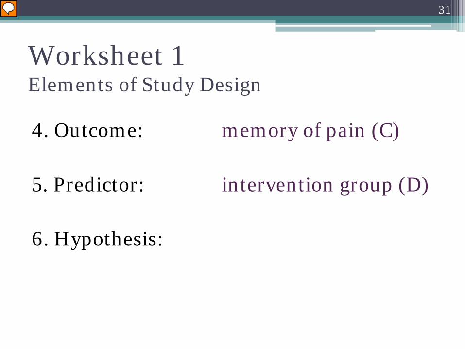
Based on the research question given in the prompt, the hypothesis can be formally stated as… Mention that this is a test as the time x intervention interaction The outcome of interest is memory of pain, a continuous variable ranging from 0 to 5.0, with 0 meaning no pain remembered and 5.0 meaning maximum pain remembered. The main predictor is intervention group, consisting of two categories, SIT and Filler. Coping style is another predictor we will account for. It has four categories, one for each possible coping style from the 2x2 table in Dr. Logan’s presentation.
30
4. Outcome:
memory of pain (C)
5. Predictor: 6. Hypothesis:
Worksheet 1 Elements of Study Design
Presenter
Presentation Notes
Based on the research question given in the prompt, the hypothesis can be formally stated as… Mention that this is a test as the time x intervention interaction The outcome of interest is memory of pain, a continuous variable ranging from 0 to 5.0, with 0 meaning no pain remembered and 5.0 meaning maximum pain remembered. The main predictor is intervention group, consisting of two categories, SIT and Filler. Coping style is another predictor we will account for. It has four categories, one for each possible coping style from the 2x2 table in Dr. Logan’s presentation.
31
4. Outcome:
memory of pain (C)
5. Predictor:
intervention group (D)
6. Hypothesis:
Worksheet 1 Elements of Study Design
Presenter
Presentation Notes
Based on the research question given in the prompt, the hypothesis can be formally stated as… Mention that this is a test as the time x intervention interaction The outcome of interest is memory of pain, a continuous variable ranging from 0 to 5.0, with 0 meaning no pain remembered and 5.0 meaning maximum pain remembered. The main predictor is intervention group, consisting of two categories, SIT and Filler. Coping style is another predictor we will account for. It has four categories, one for each possible coping style from the 2x2 table in Dr. Logan’s presentation.
32
4. Outcome:
memory of pain (C)
5. Predictor:
intervention group (D)
6. Hypothesis: time by intervention interaction (A)
Worksheet 1 Elements of Study Design
Presenter
Presentation Notes
Based on the research question given in the prompt, the hypothesis can be formally stated as… Mention that this is a test as the time x intervention interaction
GLIMMPSE is a user-friendly online tool for calculating power and sample size for multilevel and longitudinal studies.
http://glimmpse.samplesizeshop.org/
GLIMMPSE
33
Presenter
Presentation Notes
In order to calculate sample size for this study design, let’s take a look at our free, online tool.
Salient Software Features
• Free
• Requires no programming expertise
• Allows saving study designs for later use
• Also available on smartphones
34
Presenter
Presentation Notes
Optional slide. Would be nice to say features of glimmpse, but may need to remove due to time constraints. Need links to the apps on slides?
Create a Study Design
35
Presenter
Presentation Notes
Mention no internet. GLIMMPSE has three modes for entering a study design. Guided mode is used for scientists, matrix mode is for trained statisticians, and also supports uploading a previously saved study design.
Create a Study Design
Select Guided Mode
36
Presenter
Presentation Notes
Mention no internet. In order to start your study design, click on the Guided Mode.
GLIMMPSE Solving For
Select Guided Mode
37
GLIMMPSE Solving For
Select Guided Mode
Checkmark = complete Pencil = incomplete
38
GLIMMPSE Solving For
Select Guided Mode
Checkmark = complete Pencil = incomplete
39
GLIMMPSE Desired Power
40
GLIMMPSE Desired Power
Enter desired power values here and click “Add”
41
Enter desired power values here and click “Add”
GLIMMPSE Desired Power
42
GLIMMPSE Type I Error Rate
43
Presenter
Presentation Notes
mention in talk that you can try different alpha’s but may not have a strong influence on sample size for this study design?
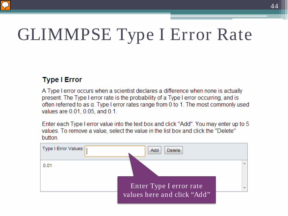
GLIMMPSE Type I Error Rate
Enter Type I error rate values here and click “Add”
44
Presenter
Presentation Notes
mention in talk that you can try different alpha’s but may not have a strong influence on sample size
Enter Type I error rate values here and click “Add”
GLIMMPSE Type I Error Rate
45
Presenter
Presentation Notes
mention in talk that you can try different alpha’s but may not have a strong influence on sample size
GLIMMPSE Predictors
46
Presenter
Presentation Notes
The primary predictor of interest is the intervention (i.e., the audio instruction for participants to use a sensory focus during their respective dental procedures). In the new study, the Iowa Dental Control Index (IDCI) will be used to categorize and select patients.14 Based on their pain coping styles, patients are classified as high desire/high felt control (i.e., high desire for control and high perceived control), high desire/low felt control, low desire/high felt control, or low desire/low felt control. Our target group is the high desire/low felt control group, which is most prone to acute dental distress. Patients in this group will be selected and randomly assigned to either intervention or no intervention. Those in the intervention group will listen to automated audio instructions to pay close attention only to the physical sensations in their mouth.9 Patients in the no intervention group will listen to automated audio instruction on a neutral topic to control for media and attention effects. As in earlier studies, appropriate manipulation checks will be used.9
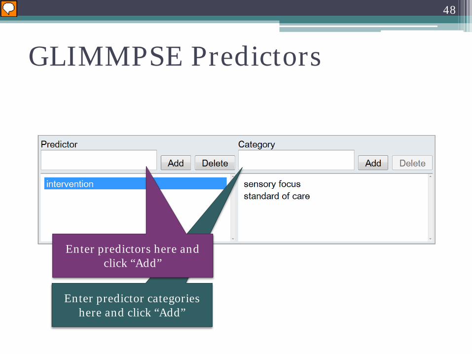
GLIMMPSE Predictors
Enter predictors here and click “Add”
47
Presenter
Presentation Notes
The primary predictor of interest is the intervention (i.e., the audio instruction for participants to use a sensory focus during their respective dental procedures). In the new study, the Iowa Dental Control Index (IDCI) will be used to categorize and select patients.14 Based on their pain coping styles, patients are classified as high desire/high felt control (i.e., high desire for control and high perceived control), high desire/low felt control, low desire/high felt control, or low desire/low felt control. Our target group is the high desire/low felt control group, which is most prone to acute dental distress. Patients in this group will be selected and randomly assigned to either intervention or no intervention. Those in the intervention group will listen to automated audio instructions to pay close attention only to the physical sensations in their mouth.9 Patients in the no intervention group will listen to automated audio instruction on a neutral topic to control for media and attention effects. As in earlier studies, appropriate manipulation checks will be used.9
Enter predictor categories here and click “Add”
Enter predictors here and click “Add”
GLIMMPSE Predictors
48
Presenter
Presentation Notes
The primary predictor of interest is the intervention (i.e., the audio instruction for participants to use a sensory focus during their respective dental procedures). In the new study, the Iowa Dental Control Index (IDCI) will be used to categorize and select patients.14 Based on their pain coping styles, patients are classified as high desire/high felt control (i.e., high desire for control and high perceived control), high desire/low felt control, low desire/high felt control, or low desire/low felt control. Our target group is the high desire/low felt control group, which is most prone to acute dental distress. Patients in this group will be selected and randomly assigned to either intervention or no intervention. Those in the intervention group will listen to automated audio instructions to pay close attention only to the physical sensations in their mouth.9 Patients in the no intervention group will listen to automated audio instruction on a neutral topic to control for media and attention effects. As in earlier studies, appropriate manipulation checks will be used.9
GLIMMPSE Outcome
49
Presenter
Presentation Notes
Mention that the outcome variable is also called the response variable.
GLIMMPSE Outcome
Enter outcomes here and click “Add”
50
Presenter
Presentation Notes
Mention that the outcome variable is also called the response variable. We measured this response variable at 3 timepoints, which we will indicate on the next screen.
Enter outcomes here and click “Add”
GLIMMPSE Outcome
51
Presenter
Presentation Notes
Mention that the outcome variable is also called the response variable.
52
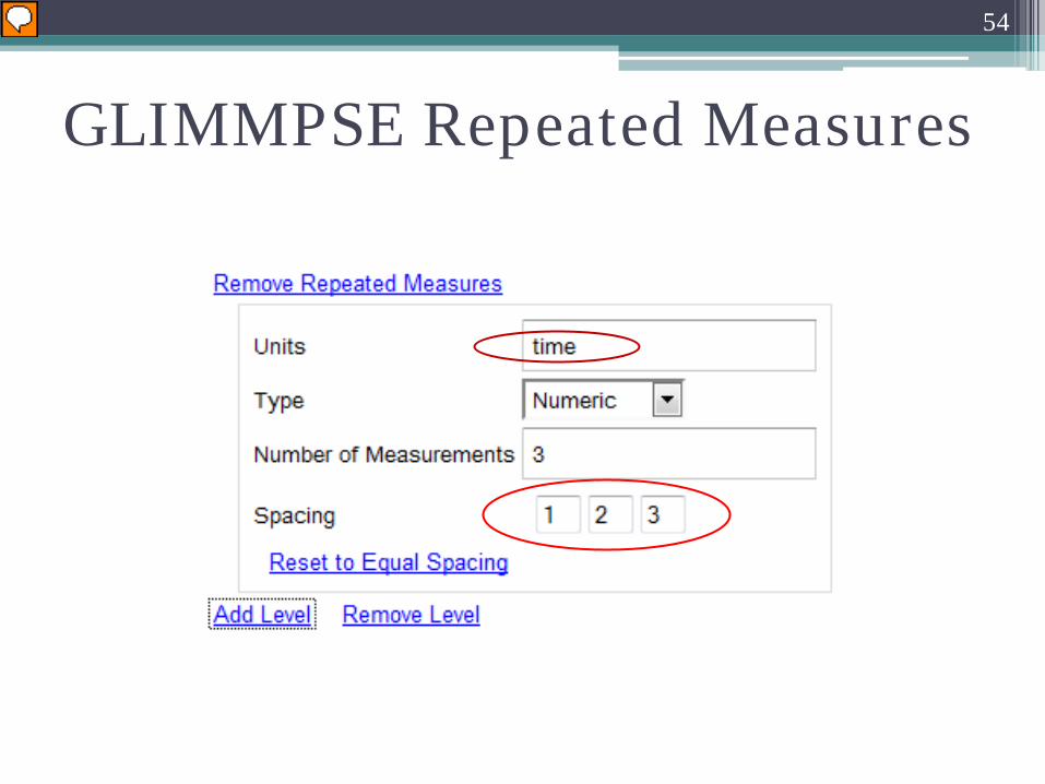
GLIMMPSE Repeated Measures
Presenter
Presentation Notes
We measure our outcome at three timepoints. Enter a label for the time variable—for instance, you could put “time” Enter that we have three measurements. Since they are evenly spaced at 6 month intervals, we can just label them timepoint 1 2 and 3.
53
GLIMMPSE Repeated Measures
Presenter
Presentation Notes
We measure our outcome at three timepoints. Enter a label for the time variable—for instance, you could put “time” Enter that we have three measurements. Since they are evenly spaced at 6 month intervals, we can just label them timepoint 1 2 and 3.
54
GLIMMPSE Repeated Measures
Presenter
Presentation Notes
We measure our outcome at three timepoints. Enter a label for the time variable—for instance, you could put “time” Enter that we have three measurements. Since they are evenly spaced at 6 month intervals, we can just label them timepoint 1 2 and 3.
GLIMMPSE Hypothesis
time by intervention interaction
55
Presenter
Presentation Notes
Recall that we want to know if the memory of pain patterns over time are different between the two intervention groups. This is called testing for a time x intervention interaction.
GLIMMPSE Hypothesis
56
Presenter
Presentation Notes
There are a number of different choices for the hypothesis. We’re going to choose “Interaction”. The interaction involves the intervention and time variables.
GLIMMPSE Hypothesis
57
Presenter
Presentation Notes
There are a number of different choices for the hypothesis. We’re going to choose “Interaction”. The interaction involves the intervention and time variables.
GLIMMPSE Hypothesis
58
Presenter
Presentation Notes
There are a number of different choices for the hypothesis. We’re going to choose “Interaction”. The interaction involves the intervention and time variables.
GLIMMPSE Hypothesis
59
Presenter
Presentation Notes
There are a number of different choices for the hypothesis. We’re going to choose “Interaction”. The interaction involves the intervention and time variables.
• Pilot study
• Similar published research
• Unpublished internal studies
• Clinical experience
60
Where Can I Find Means, Variances, and Correlations?
Presenter
Presentation Notes
In order to complete the power analysis, we need to predict what we will get for our means, variances, and correlations if we actually ran the study. Where can we find the means, variances, and correlations? We find them from these places…
• Mean: a measure of the size of the intervention effect
• Variance: a measure of the variability of the outcome
• Correlation: a measure of the association between the repeated measures
Worksheet 2 Means, Variances, and Correlations
61
Presenter
Presentation Notes
Break into small groups and turn to Worksheet 2. Based on the information on Worksheet 2, specify the expected means, variances, and correlations for the planned memory of pain study. Here are definitions of the mean, variance, and correlation as they relate to our planned study.
Agenda
62
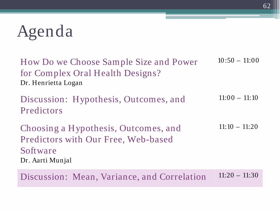
How Do we Choose Sample Size and Power for Complex Oral Health Designs? Dr. Henrietta Logan
10:50 – 11:00
Discussion: Hypothesis, Outcomes, and Predictors
11:00 – 11:10
Choosing a Hypothesis, Outcomes, and Predictors with Our Free, Web-based Software Dr. Aarti Munjal
11:10 – 11:20
Discussion: Mean, Variance, and Correlation
11:20 – 11:30
Agenda
63
Choosing Means, Variances, and Correlations with Our Free, Web-based Software Brandy M. Ringham
11:30 – 11:40
Discussion: Sample Size Calculation Summary
11:40 – 11:50
Wrapping it Up: Writing the Grant Deborah H. Glueck
11:50 – 12:00
Discussion: Question and Answer 12:00 – 12:15
64
Choosing Means, Variances, and Correlations with Our Free,
Web-based Software
Brandy Ringham University of Colorado Denver
Worksheet 2 Means, Variances, and Correlations
65
Correlation Between Outcomes Over Time Gedney, Logan, and Baron (2003) identified predictors of the amount of experienced pain recalled over time…One of the findings was that memory of pain intensity at 1 week and 18 months had a correlation of 0.4. …assume that the correlation between measures 18 months apart will be similar to the correlation between measures 12 months apart. Likewise, the correlation between measures 6 months apart will be only slightly greater than the correlation between measures 18 months apart.
Worksheet 2 Means, Variances, and Correlations
66
Correlation Between Outcomes Over Time Gedney, Logan, and Baron (2003) identified predictors of the amount of experienced pain recalled over time…One of the findings was that memory of pain intensity at 1 week and 18 months had a correlation of 0.4. …assume that the correlation between measures 18 months apart will be similar to the correlation between measures 12 months apart. Likewise, the correlation between measures 6 months apart will be only slightly greater than the correlation between measures 18 months apart.
Worksheet 2 Means, Variances, and Correlations
67
Correlation Between Outcomes Over Time Gedney, Logan, and Baron (2003) identified predictors of the amount of experienced pain recalled over time…One of the findings was that memory of pain intensity at 1 week and 18 months had a correlation of 0.4. …assume that the correlation between measures 18 months apart will be similar to the correlation between measures 12 months apart. Likewise, the correlation between measures 6 months apart will be only slightly greater than the correlation between measures 18 months apart.
Correlation at 6 months apart
Correlation at 12 months apart
Worksheet 2 Means, Variances, and Correlations
68
(A)
(B)
Correlation at 6 months apart
Correlation at 12 months apart
Worksheet 2 Means, Variances, and Correlations
69
(A)
(B) 0.4
Presenter
Presentation Notes
Break into small groups and turn to Worksheet 2. Based on the information on Worksheet 2, specify the expected means, variances, and correlations for the planned memory of pain study. Recall that…
Worksheet 2 Means, Variances, and Correlations
70
Correlation Between Outcomes Over Time Gedney, Logan, and Baron (2003) identified predictors of the amount of experienced pain recalled over time…One of the findings was that memory of pain intensity at 1 week and 18 months had a correlation of 0.4. …assume that the correlation between measures 18 months apart will be similar to the correlation between measures 12 months apart. Likewise, the correlation between measures 6 months apart will be only slightly greater than the correlation between measures 18 months apart.
Presenter
Presentation Notes
Break into small groups and turn to Worksheet 2. Based on the information on Worksheet 2, specify the expected means, variances, and correlations for the planned memory of pain study. Recall that…
Worksheet 2 Means, Variances, and Correlations
71
Correlation Between Outcomes Over Time Gedney, Logan, and Baron (2003) identified predictors of the amount of experienced pain recalled over time…One of the findings was that memory of pain intensity at 1 week and 18 months had a correlation of 0.4. …assume that the correlation between measures 18 months apart will be similar to the correlation between measures 12 months apart. Likewise, the correlation between measures 6 months apart will be only slightly greater than the correlation between measures 18 months apart.
Presenter
Presentation Notes
Break into small groups and turn to Worksheet 2. Based on the information on Worksheet 2, specify the expected means, variances, and correlations for the planned memory of pain study. Recall that…
Correlation at 6 months apart
Correlation at 12 months apart
Worksheet 2 Means, Variances, and Correlations
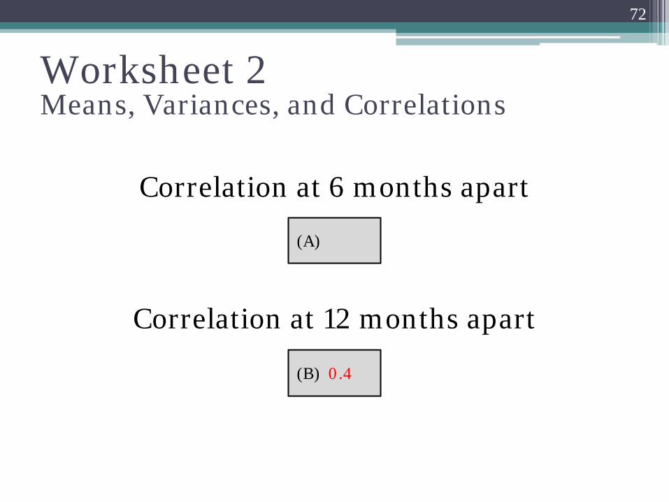
72
(A)
(B) 0.4
Correlation at 6 months apart
Correlation at 12 months apart
Worksheet 2 Means, Variances, and Correlations
73
(A) 0.5
(B) 0.4
Worksheet 2 Means, Variances, and Correlations
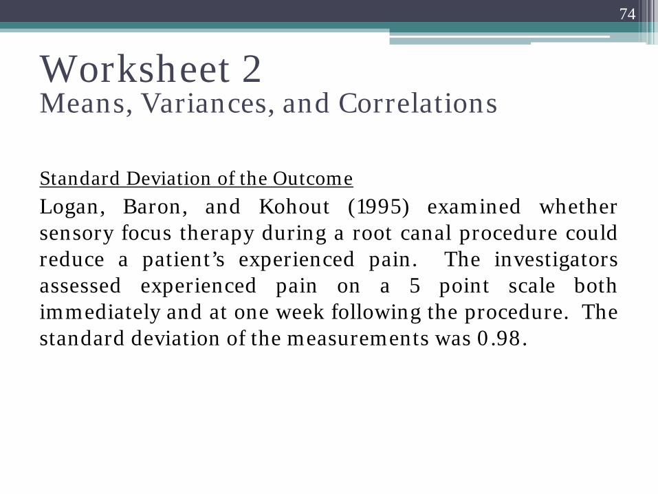
74
Standard Deviation of the Outcome Logan, Baron, and Kohout (1995) examined whether sensory focus therapy during a root canal procedure could reduce a patient’s experienced pain. The investigators assessed experienced pain on a 5 point scale both immediately and at one week following the procedure. The standard deviation of the measurements was 0.98.
Worksheet 2 Means, Variances, and Correlations
75
Standard Deviation of the Outcome Logan, Baron, and Kohout (1995) examined whether sensory focus therapy during a root canal procedure could reduce a patient’s experienced pain. The investigators assessed experienced pain on a 5 point scale both immediately and at one week following the procedure. The standard deviation of the measurements was 0.98.
Standard deviation of memory of pain
Worksheet 2 Means, Variances, and Correlations
76
(C)
Standard deviation of memory of pain
Worksheet 2 Means, Variances, and Correlations
77
(C) 0.98
Worksheet 2 Means, Variances, and Correlations
78
Intervention Baseline 6 Months 12 Months
Sensory Focus (SF)
3.6 2.8 0.9
Standard of Care
(SOC) 4.5 4.3 3.0
Intervention Difference
(SF - SOC)
Net Difference Over Time
(12 Months - Baseline)
(D) -0.9 (E) -1.5 (F) -2.1
(G) -1.2
Worksheet 2 Means, Variances, and Correlations
79
Intervention Baseline 6 Months 12 Months
Sensory Focus (SF)
3.6 2.8 0.9
Standard of Care
(SOC) 4.5 4.3 3.0
Intervention Difference
(SF - SOC)
Net Difference Over Time
(12 Months - Baseline)
(D) -0.9 (E) -1.5 (F) -2.1
(G) -1.2
Worksheet 2 Means, Variances, and Correlations
80
Intervention Baseline 6 Months 12 Months
Sensory Focus (SF)
3.6 2.8 0.9
Standard of Care
(SOC) 4.5 4.3 3.0
Intervention Difference
(SF - SOC)
Net Difference Over Time
(12 Months - Baseline)
(D) -0.9 (E) -1.5 (F) -2.1
(G) -1.2
Worksheet 2 Means, Variances, and Correlations
81
Intervention Baseline 6 Months 12 Months
Sensory Focus (SF)
3.6 2.8 0.9
Standard of Care
(SOC) 4.5 4.3 3.0
Intervention Difference
(SF - SOC)
Net Difference Over Time
(12 Months - Baseline)
(D) -0.9 (E) -1.5 (F) -2.1
(G) -1.2
Worksheet 2 Means, Variances, and Correlations
82
Intervention Baseline 6 Months 12 Months
Sensory Focus (SF)
3.6 2.8 0.9
Standard of Care
(SOC) 4.5 4.3 3.0
Intervention Difference
(SF - SOC)
Net Difference Over Time
(12 Months - Baseline)
(D) -0.9 (E) -1.5 (F) -2.1
(G) -1.2
83
GLIMMPSE Means Specifying a Mean Difference
84
GLIMMPSE Means Specifying a Mean Difference
Choose a timepoint
85
Enter the expected net mean difference
GLIMMPSE Means Specifying a Mean Difference
Choose a timepoint
86
GLIMMPSE Variability Entering Standard Deviation of the Outcome
87
GLIMMPSE Variability Entering Standard Deviation of the Outcome
Enter the standard deviation of the outcome variable
Enter the standard deviation of the outcome variable
88
GLIMMPSE Variability Specifying Correlations
Presenter
Presentation Notes
The investigators suggested that the variance of a change in pain was Var(Di) = 0.96 Correlations between difference values were Corr(D1,D2) = 0.5 Corr(D2,D3) = 0.4 GLIMMPSE allows various ways of entering covariance information. Above shows the lear model. This model allows correlation to decay as the time between the measurements increases. Above we have selected a decay rate of 0.3, so that the correlation decay matches the values determined by the investigators. Alternatively, we could enter the correlation values directly using the custom correlation view
89
GLIMMPSE Variability Specifying Correlations
Enter correlations between repeated measures
Presenter
Presentation Notes
The investigators suggested that the variance of a change in pain was Var(Di) = 0.96 Correlations between difference values were Corr(D1,D2) = 0.5 Corr(D2,D3) = 0.4
90
GLIMMPSE Hypothesis Test
Presenter
Presentation Notes
In the case of repeated measures, several different statistical tests are available. These tests use slightly different approximation methods when calculating power. Results will be similar but may yield slightly different sample sizes. Note that it is important that the same test is used for data analysis as was used for the sample size calculation. Glimmpse has tutorials on this.
91
GLIMMPSE Hypothesis Test
Presenter
Presentation Notes
In the case of repeated measures, several different statistical tests are available. These tests use slightly different approximation methods when calculating power. Results will be similar but may yield slightly different sample sizes. Note that it is important that the same test is used for data analysis as was used for the sample size calculation. Glimmpse has tutorials on this.
92
GLIMMPSE Hypothesis Test
Presenter
Presentation Notes
In the case of repeated measures, several different statistical tests are available. These tests use slightly different approximation methods when calculating power. Results will be similar but may yield slightly different sample sizes. Note that it is important that the same test is used for data analysis as was used for the sample size calculation. Glimmpse has tutorials on this.
93
GLIMMPSE Calculate Button
Presenter
Presentation Notes
When a complete study design has been entered, the calculate button will highlight Click the calculate button to obtain your results
94
GLIMMPSE Results
Presenter
Presentation Notes
Displays the total sample size required to achieve 90% power. This column shows the sample size needed to achieve 90% power. Why are there three sample sizes? Look at the sigma scale column. GLIMMPSE allows you to enter “scale factors” to scale the variance to ½ or 2 times what you expected. This is useful if you are unsure what the variance will be. This first row is the variance we originally entered (.98). The other two rows show how the sample size is affected when you change the variance. Also allows user to view the underlying matrices in the calculation (to verify that the correct contrast is used, for example) Allows user to save the results to a CSV file
95
Total sample size to achieve at least 90% power
GLIMMPSE Results
Presenter
Presentation Notes
Displays the total sample size required to achieve 90% power. This column shows the sample size needed to achieve 90% power. Why are there three sample sizes? Look at the sigma scale column. GLIMMPSE allows you to enter “scale factors” to scale the variance to ½ or 2 times what you expected. This is useful if you are unsure what the variance will be. This first row is the variance we originally entered (.98). The other two rows show how the sample size is affected when you change the variance. Also allows user to view the underlying matrices in the calculation (to verify that the correct contrast is used, for example) Allows user to save the results to a CSV file
Total sample size to achieve at least 90% power
96
Scale the standard deviation to ½ and 2 times to see how it affects
sample size
GLIMMPSE Results
Presenter
Presentation Notes
Displays the total sample size required to achieve 90% power. This column shows the sample size needed to achieve 90% power. Why are there three sample sizes? Look at the sigma scale column. GLIMMPSE allows you to enter “scale factors” to scale the variance to ½ or 2 times what you expected. This is useful if you are unsure what the variance will be. This first row is the variance we originally entered (.98). The other two rows show how the sample size is affected when you change the variance. Also allows user to view the underlying matrices in the calculation (to verify that the correct contrast is used, for example) Allows user to save the results to a CSV file
Total sample size to achieve at least 90% power
Scale the standard deviation to ½ and 2 times to see how it affects
sample size
97
GLIMMPSE Results
Presenter
Presentation Notes
Displays the total sample size required to achieve 90% power. This column shows the sample size needed to achieve 90% power. Why are there three sample sizes? Look at the sigma scale column. GLIMMPSE allows you to enter “scale factors” to scale the variance to ½ or 2 times what you expected. This is useful if you are unsure what the variance will be. This first row is the variance we originally entered (.98). The other two rows show how the sample size is affected when you change the variance. Also allows user to view the underlying matrices in the calculation (to verify that the correct contrast is used, for example) Allows user to save the results to a CSV file
98
Funding the Planned Study
Presenter
Presentation Notes
You’ve now planned your entire study, including completing your sample size calculation. You want to secure funding for the study so you are going to apply for a grant. Grant applications require you to justify the planned enrollment. This justification includes a summary of the sample size calculation.
• Summarize the sample size calculation
• Include the following information: • Type I error rate • Desired power • Hypothesis • Hypothesis test used • Analysis method • Means, variances, correlation with justification • Calculated sample size
99
Worksheet 3 Sample Size Calculation Summary
Presenter
Presentation Notes
You’ve now planned your entire study, including completing your sample size calculation. You want to secure funding for the study so you are going to apply for a grant. Grant applications require you to justify the planned enrollment. This justification includes a summary of the sample size calculation.
Agenda
100
Choosing Means, Variances, and Correlations with Our Free, Web-based Software Brandy M. Ringham
11:30 – 11:40
Discussion: Sample Size Calculation Summary
11:40 – 11:50
Wrapping it Up: Writing the Grant Deborah H. Glueck
11:50 – 12:00
Discussion: Question and Answer 12:00 – 12:15
Agenda
101
Choosing Means, Variances, and Correlations with Our Free, Web-based Software Brandy M. Ringham
11:30 – 11:40
Discussion: Sample Size Calculation Summary
11:40 – 11:50
Wrapping it Up: Writing the Grant Deborah H. Glueck
11:50 – 12:00
Discussion: Question and Answer 12:00 – 12:15
102
Wrapping it Up: Writing the Grant
Dr. Deborah Glueck University of Colorado Denver
• Aligning power analysis with data analysis • Justifying the power analysis • Accounting for uncertainty • Handling missing data • Demonstrating enrollment feasibility • Planning for multiple aims
103
Outline Writing the Grant
We plan a repeated measures ANOVA using the Hotelling-Lawley Trace to test for a time by intervention interaction.
104
Worksheet 3 Sample Size Calculation Summary
We plan a repeated measures ANOVA using the Hotelling-Lawley Trace to test for a time by intervention interaction.
105
Worksheet 3 Sample Size Calculation Summary
• Type I error rate • α = 0.01
• Hypothesis test • Wrong: power = intervention data analysis = time x intervention
• Right: power = time x intervention data analysis = time x intervention
106
Aligning Power Analysis with Data Analysis
Presenter
Presentation Notes
Power analysis should be aligned with the planned data analysis. If you conduct a power analysis for a Type I error rate of 0.01, you should use p-values of 0.01 as your threshold for significance in the data analysis (is this true). If you conduct a power analysis for a hypothesis of time x intervention interaction using a repeated measures ANOVA and the Hotelling-Lawley trace, then that should be the data analysis that you do. So what if you have a study where you want to test multiple hypotheses? How do you match the power analysis to the data analysis?
Based on previous studies, we predict memory of pain measures will have a standard deviation of 0.98 and the correlation between baseline and 6 months will be 0.5. Based on clinical experience, we believe the correlation will decrease slowly over time, for a correlation of 0.4 between pain recall measures at baseline and 12 months.
107
Worksheet 3 Sample Size Calculation Summary
Based on previous studies, we predict memory of pain measures will have a standard deviation of 0.98 and the correlation between baseline and 6 months will be 0.5. Based on clinical experience, we believe the correlation will decrease slowly over time, for a correlation of 0.4 between pain recall measures at baseline and 12 months.
108
Worksheet 3 Sample Size Calculation Summary
• Give all the values needed to recreate the power analysis
• Provide appropriate citation
109
Justifying the Power Analysis
Presenter
Presentation Notes
Power analysis should be aligned with the planned data analysis. If you conduct a power analysis for a Type I error rate of 0.01, you should use p-values of 0.01 as your threshold for significance in the data analysis (is this true). If you conduct a power analysis for a hypothesis of time x intervention interaction using a repeated measures ANOVA and the Hotelling-Lawley trace, then that should be the data analysis that you do. So what if you have a study where you want to test multiple hypotheses? How do you match the power analysis to the data analysis?
For a desired power of 0.90 and a Type I error rate of 0.01, we estimated that we would need 44 participants to detect a clinically meaningful mean difference of 1.2.
110
Worksheet 3 Sample Size Calculation Summary
For a desired power of 0.90 and a Type I error rate of 0.01, we estimated that we would need 44 participants to detect a clinically meaningful mean difference of 1.2.
111
Worksheet 3 Sample Size Calculation Summary
Pow
er
112
Accounting for Uncertainty
Mean Difference
Pow
er
Mean Difference
113
0.90
Accounting for Uncertainty
Pow
er
Mean Difference
0.90
114
Accounting for Uncertainty
We plan a repeated measures ANOVA using the Hotelling-Lawley Trace to test for a time by intervention interaction. Based on previous studies, we predict measures of pain recall will have a standard deviation of 0.98. The correlation in pain recall between baseline and 6 months will be 0.5. Based on clinical experience, we predict that the correlation will decrease slowly over time. Thus, we anticipate a correlation of 0.4 between pain recall measures at baseline and 12 months. For a desired power of 0.90 and a Type I error rate of 0.01, we need to enroll 44 participants to detect a clinically meaningful mean difference of 1.2.
115
Worksheet 3 Sample Size Calculation Summary Draft
Presenter
Presentation Notes
But wait! There’s always another draft of the grant.
• 25% loss to follow-up
• Account for missing data by increasing the sample size
44 / 0.75 = 59
116
Handling Missing Data
Presenter
Presentation Notes
We inflate the calculated sample size. We expect to lose 25% of people. We want the sample size to be at least 44 after we lose the participants. We need to calculate the sample size we should start with in order to have 44 people left after one year. 44 = X x 0.75 or X = 44 / 0.75 = 59. This gives us a target sample size of 59. But this is the total sample size. Since we need to divide the sample size evenly between the two intervention groups, we increase it by 1 for a target sample size of 60.
• 25% loss to follow-up
• Account for missing data by increasing the sample size
44 / 0.75 ≈ 60
117
Handling Missing Data
Presenter
Presentation Notes
We inflate the calculated sample size. We expect to lose 25% of people. We want the sample size to be at least 44 after we lose the participants. We need to calculate the sample size we should start with in order to have 44 people left after one year. 44 = X x 0.75 or X = 44 / 0.75 = 59. This gives us a target sample size of 59. But this is the total sample size. Since we need to divide the sample size evenly between the two intervention groups, we increase it by 1 for a target sample size of 60.
Over 12 months, we expect 25% loss to follow up. To account for attrition, we will increase the sample size to 60 participants, or 30 participants per intervention arm.
118
Worksheet 3 Sample Size Calculation Summary
Over 12 months, we expect 25% loss to follow up. To account for attrition, we will increase the sample size to 60 participants, or 30 participants per intervention arm.
119
Worksheet 3 Sample Size Calculation Summary
• Is the target population sufficiently large?
• Can recruitment be completed in the proposed time period?
120
Demonstrating Enrollment Feasibility
Presenter
Presentation Notes
The power analysis section should also discuss the practicality of your enrollment goal. Is the target population large enough? Can you complete the recruitment in the proposed amount of time?
• 30 patients per week with a high desire / low felt coping style
• 40% consent rate
121
Sample size needed 60
Sample size available
Planned Sample Size vs. Available Sample Size
Presenter
Presentation Notes
How do we come up with a realistic enrollment goal? Let’s say we propose to enroll 60 participants total over a 3 week period. Recall that Dr. Logan told us the characteristics of her study population. She sees about 30 patients per week with a high desire/low felt coping style. When she does recruitment in her clinic, she typically gets a 40% consent rate. At 30 patients / week and a 40% consent rate, Dr. Logan can enroll only 12 patients per week. Over three weeks, that’s only 36 participants. This is not a realistic enrollment goal. Instead, we should propose a longer enrollment period so we can reach our planned sample size. If we plan to enroll participants for 5 weeks, we could reach 60 participants.
• 30 patients per week with a high desire / low felt coping style
• 40% consent rate
122
Sample size needed 60
Sample size available 36
Planned Sample Size vs. Available Sample Size
3 week enrollment period
Presenter
Presentation Notes
How do we come up with a realistic enrollment goal? Let’s say we propose to enroll 60 participants total over a 3 week period. Recall that Dr. Logan told us the characteristics of her study population. She sees about 30 patients per week with a high desire/low felt coping style. When she does recruitment in her clinic, she typically gets a 40% consent rate. At 30 patients / week and a 40% consent rate, Dr. Logan can enroll only 12 patients per week. Over three weeks, that’s only 36 participants. This is not a realistic enrollment goal. Instead, we should propose a longer enrollment period so we can reach our planned sample size. If we plan to enroll participants for 5 weeks, we could reach 60 participants.
• 30 patients per week with a high desire / low felt coping style
• 40% consent rate
123
Sample size needed 60
Sample size available 60
Planned Sample Size vs. Available Sample Size
5 week enrollment period
Presenter
Presentation Notes
How do we come up with a realistic enrollment goal? Let’s say we propose to enroll 60 participants total over a 3 week period. Recall that Dr. Logan told us the characteristics of her study population. She sees about 30 patients per week with a high desire/low felt coping style. When she does recruitment in her clinic, she typically gets a 40% consent rate. At 30 patients / week and a 40% consent rate, Dr. Logan can enroll only 12 patients per week. Over three weeks, that’s only 36 participants. This is not a realistic enrollment goal. Instead, we should propose a longer enrollment period so we can reach our planned sample size. If we plan to enroll participants for 5 weeks, we could reach 60 participants.
The clinic treats 30 patients per week with the high desire/low felt coping style. Based on recruitment experience for previous studies, we expect a 40% consent rate. At an effective enrollment of 12 participants per week, we will reach the enrollment goal of 60 participants in 5 weeks time.
124
Worksheet 3 Sample Size Calculation Summary
The clinic treats 30 patients per week with the high desire/low felt coping style. Based on recruitment experience for previous studies, we expect a 40% consent rate. At an effective enrollment of 12 participants per week, we will reach the enrollment goal of 60 participants in 5 weeks time.
125
Worksheet 3 Sample Size Calculation Summary
• Aims typically represent different hypotheses
• Maximum of the sample sizes calculated for each aim
126
Planning for Multiple Aims
127
Questions?
• How do I find GLIMMPSE?
• How can I put it on my smartphone?
• Can you review a point from the example power analysis?
128
Question & Answer
Adams, G., Gulliford, M. C., Ukoumunne, O. C., Eldridge, S., Chinn, S., & Campbell, M. J. (2004). Patterns of intra-cluster correlation from primary care research to inform study design and analysis. Journal of clinical epidemiology, 57(8), 785-794.
Catellier, D. J., & Muller, K. E. (2000). Tests for gaussian repeated measures with missing data in small samples. Statistics in Medicine, 19(8), 1101-1114.
Demidenko, E. (2004). Mixed Models: Theory and Applications (1st ed.). Wiley-Interscience.
Glueck, D. H., & Muller, K. E. (2003). Adjusting power for a baseline covariate in linear models. Statistics in Medicine, 22, 2535-2551.
129
References
Gedney , J.J., Logan, H.L., Baron, R.S. (2003). Predictors of short-term and long-term memory of sensory and affective dimensions of pain. Journal of Pain, 4(2), 47–55.
Gedney, J.J., Logan H.L. (2004). Memory for stress-associated acute pain. Journal of Pain, 5(2), 83–91.
Gurka, M. J., Edwards, L. J., & Muller, K. E. (2011). Avoiding bias in mixed model inference for fixed effects. Statistics in Medicine, 30(22), 2696-2707. doi:10.1002/sim.4293
Kerry, S. M., & Bland, J. M. (1998). The intracluster correlation coefficient in cluster randomisation. BMJ (Clinical research ed.), 316(7142), 1455.
130
References
Kreidler, S.M., Muller, K.E., Grunwald, G.K., Ringham, B.M., Coker-Dukowitz, Z.T., Sakhadeo, U.R., Barón, A.E., Glueck, D.H. (accepted). GLIMMPSE: Online Power Computation for Linear Models With and Without a Baseline Covariate. Journal of Statistical Software.
Laird, N. M., & Ware, J. H. (1982). Random-effects models for longitudinal data. Biometrics, 38(4), 963-974.
Law, A., Logan, H., & Baron, R. S. (1994). Desire for control, felt control, and stress inoculation training during dental treatment. Journal of Personality and Social Psychology, 67(5), 926-936.
Logan, H.L., Baron, R.S., Keeley, K., Law, A., Stein, S. (1991). Desired control and felt control as mediators of stress in a dental setting. Health Psychology, 10(5), 352–359.
131
References
Logan, H.L., Baron, R.S., Kohout, F. (1995). Sensory focus as therapeutic treatments for acute pain. Psychosomatic Medicine, 57(5), 475–484.
Muller, K. E, & Barton, C. N. (1989). Approximate Power for Repeated-Measures ANOVA Lacking Sphericity. Journal of the American Statistical Association, 84(406), 549-555.
Muller, K. E, Edwards, L. J., Simpson, S. L., & Taylor, D. J. (2007). Statistical Tests with Accurate Size and Power for Balanced Linear Mixed Models. Statistics in Medicine, 26(19), 3639-3660.
Muller, K. E, Lavange, L. M., Ramey, S. L., & Ramey, C. T. (1992). Power Calculations for General Linear Multivariate Models Including Repeated Measures Applications. Journal of the American Statistical Association, 87(420), 1209-1226.
132
References
Muller, K. E, & Peterson, B. L. (1984). Practical Methods for Computing Power in Testing the Multivariate General Linear Hypothesis. Computational Statistics and Data Analysis, 2, 143-158.
Muller, K.E., & Stewart, P. W. (2006). Linear Model Theory: Univariate, Multivariate, and Mixed Models. Hoboken, NJ: Wiley.
Taylor, D. J., & Muller, K. E. (1995). Computing Confidence Bounds for Power and Sample Size of the General Linear Univariate Model. The American Statistician, 49(1), 43-47. doi:10.2307/2684810


![e HELP - Panasonic HELP English TH-58DX900U TH ... • HDMI HDR Setting [This feature is available depending on your model.] 64 • Valid input signals 65 ... • Selecting file 140](https://img.dokumen.tips/doc/110x75/5b0a413c7f8b9abe5d8df52e/e-help-panasonic-help-english-th-58dx900u-th-hdmi-hdr-setting-this-feature.jpg)