Selected Indicators of Financial Stability · Selected Indicators of Financial Stability ... assisting in the formulation and implementation of policies regarding Reserve Banks' credit

- 1 -

Selected Indicators of Financial Stability William R. Nelson and Roberto Perli† Monetary and Financial Stability Section Division of Monetary Affairs Federal Reserve Board

1. Introduction

The stability of the financial system, as evidenced by markets that are functioning well,

by key institutions that are operating without major difficulty, and by asset prices that are

not significantly removed from fundamental values, is vital if an economy is to achieve

the objectives of sustained growth and low inflation. A financial system that is stable

will also be resilient and will be able to withstand normal fluctuations in asset prices that

result from dynamic demand and supply conditions, as well as substantial increases in

uncertainty. Financial instability, on the other hand, can impede economic activity and

reduce economic welfare. If financial markets become dysfunctional or the condition of

key institutions becomes severely strained, the attendant pressures on businesses and

households may have adverse effects on the real economy as capital may be prevented

from flowing to worthy investments and credit crunches may develop. To the extent that

those pressures are judged to be sufficiently acute, policymakers may want to respond by

altering the stance of monetary policy. Conversely, economic and monetary policy

surprises can trigger financial instability and compromise the effectiveness of the

† The views expressed in this paper are those of the authors and not those of the Board of Governors of the Federal Reserve System. Nelson: [email protected], mail stop 74, Federal Reserve Board, Washington, DC 20551. Perli: [email protected], mail stop 75, Federal Reserve Board, Washington, DC 20551. Andrea Surratt provided excellent research assistance. A previous version of this paper was presented at the Irving Fisher Committee’s Workshop on Data Requirements for Analysing the Stability and Vulnerability of Mature Financial Systems, Bank of Canada, Ottawa, June 2005. The authors would like to thank participants to that workshop, as well as several of their Board colleagues, for their comments and suggestions.

- 2 -

monetary policy transmission mechanism. As markets react to the new information, large

and sudden price movements may occur that may lead to substantial losses and to

heightened uncertainty and unwillingness to take on risk. Because of the

interdependency between the financial system, the state of the economy, and monetary

policy, monitoring financial markets and appropriately assessing their stability are tasks

of great importance to policymakers. Indeed, the staff of the Federal Reserve Board

devotes a significant amount of time and resources to assess the overall health of the

financial system and, when financial disturbances occur, to judge the implications of

those disturbances for the nonfinancial sector.

The rapid pace of financial innovation that has taken place over the course of the

last decade has brought about a proliferation of new and increasingly sophisticated

financial products, has led to the appearance of new types of institutions, and has created

new and expanded roles for existing institutions. Against this backdrop of increased

complexity, key goals of the Board’s staff are to understand financial markets as well as

possible and to be able to identify in a timely fashion the potential consequences of any

new developments. In pursuit of those objectives, the staff relies on its expertise and

judgment, on market intelligence, and on a broad range of financial indicators. Many of

those indicators are measures of financial strength, that is, measures of the ability of

households or businesses to weather shocks without greatly contracting their spending.

Other measures focus on market participants’ assessments of, and appetite for, risk.

Individual indicators are also combined into aggregate measures that give a synthetic

picture of overall financial conditions and thus summarize the general stability of the

financial system. While notable efforts have been made in the academic literature as well

as at other institutions to develop indicators that could be predictive of adverse

developments, all indicators in use at the Board are contemporaneous in nature and are

used purely as tools to help interpret current conditions.1 And importantly, neither the

1 Reviews and discussions of the predictive ability of various types of indicators, as applied to different types of crises, are contained, for example, in Berg, A. and Pattillo, C., “Are Currency Crises Predictable? A Test,” IMF Staff Papers vol. 46, no. 2, June 1999, and Kumar, M.S. and Persaud, A., “Pure Contagion and Investors’ Shifting Risk Appetite: Analytical Issues and Empirical Evidence,” IMF Working Paper no. 134, 2001.

- 3 -

individual nor the aggregate measures are used as “black boxes” to determine policy

actions; rather, they are just a few among a host of instruments that the Board’s staff

draws on to inform policy makers of the current state of financial markets.

The individual measures of financial stability used by the Board’s staff are taken

from a variety of sources, and are available at a wide range of frequencies. Some, such as

asset prices, are market-based and can be calculated daily, if not even more frequently.

Others, such as financial stocks and flows, are aggregated from individual institutions at a

weekly, monthly, or quarterly basis. Finally, some measures are based on surveys, both

formal and informal, of market participants, and are gathered on an ongoing basis. The

Board of Governors is provided updates about financial market developments often (at

least weekly and sometimes more frequently). The Federal Open Market Committee,

which sets the overnight interbank (federal funds) rate in the United States, is provided

with information on financial conditions before each FOMC meeting, although many

measures are also provided to Committee members on a more frequent basis. Reports on

the functioning of U.S. financial markets are prepared at regular intervals in advance of

international meetings on financial stability. Several Divisions at the Federal Reserve

Board, including the Divisions of Monetary Affairs, Research and Statistics, International

Finance, Bank Supervision and Regulation, and Reserve Bank Operations and Payment

Systems, contribute to the compilation and interpretation of this information.

While the focus of this paper is on quantitative gauges of financial stability, we

should note that qualitative information also figures prominently in the set of tools Board

economists use to assess the state of the financial system. Formal surveys of investors

and bank senior loan officers are conducted regularly and provide timely information on

the respondents’ views on current developments and their likely future unfolding. More

informal contacts with market participants, either direct or through the Open Market

Desk of the Federal Reserve Bank of New York, are instrumental in the interpretation of

the vast amount of information that is received on any given day. Market contacts are

especially valuable when events are unfolding rapidly and there is no time to wait for

responses to formal surveys. Of course, qualitative information that is received from

- 4 -

market participants needs to be evaluated, put in context, and possibly filtered, but has

nonetheless repeatedly proved useful in the past.

Sections 2 to 6 of this paper summarize some of the individual and aggregate

indicators that are monitored by the authors and other members of the Board’s staff.2

Section 7 briefly discusses how some of those indicators were used to assess the impact

of the turmoil in the credit markets in the spring of 2005 that was induced by the credit

quality deterioration of two large U.S. automobile manufacturers, and section 8 contains

some conclusive thoughts.

2. Measures based on interest rates and asset prices

Asset prices and interest rates are determined by the supplies and demands of forward-

looking investors and savers; as such, they react nearly instantaneously to investors’

judgments about financial conditions. Because many prices and rates are available

virtually instantaneously and continuously, Board staff members monitor a broad range

of them for prompt information on market liquidity and market participants’ attitudes

toward risk.3

Measures of market liquidity provide information on the ability of financial

markets to absorb large transactions without large changes in prices, and on the premiums

investors are willing to pay to hold more liquid assets. The Board’s staff assesses the

liquidity of the market for U.S. Treasury securities, in part, by looking at bid-ask spreads

and volumes. As an example, the top two panels of exhibit 1 plot these measures for the

2 The authors are part of the Monetary and Financial Stability section (MFST) of the Division of Monetary Affairs (MA). MFST is responsible for analyzing a variety of issues related to financial stability and the operation of financial institutions and markets. Key areas of specialization include the collection and evaluation of information on financial institutions, methods for assessing stress in financial markets, and assisting in the formulation and implementation of policies regarding Reserve Banks' credit and risk management. Section economists analyze financial developments for the Board of Governors and the FOMC and engage in a broad range of longer-term research projects. Not all the measures discussed in this paper are produced by MFST or MA. 3 This paper draws, in part, from “Pragmatic Monitoring of Financial Stability,” by William R. Nelson and Wayne Passmore, in Marrying the Macro- and Micro-Prudential Dimensions of Financial Stability, BIS Papers, No.1, March 2001. That paper contains, among other things, a more detailed description of some of the individual indicators of financial stability in use at the time at the Federal Reserve Board.

- 5 -

ten-year on-the-run Treasury security in April and early May, 2005.4 The Treasury

market is an over-the-counter (OTC) market, and consequently bid-ask spreads and

volume data for Treasury securities are more difficult to obtain than for exchange-traded

securities, such as stocks or most futures. The Board’s staff currently relies on intraday

data collected by electronic brokers, such as BrokerTec for the interdealer market and

TradeWeb for the dealer-to-customer market. While those electronic brokers do not

represent the whole market, they appear to account for substantial and growing

percentages of the total daily trading volumes in Treasury securities.

[Exhibit 1 about here]

Members of the Board’s staff also follow liquidity premiums, defined as the yield

on a less liquid security minus the yield on a highly liquid but otherwise similar security.

Highly liquid securities, generally, can be sold rapidly and at a known price. The amount

investors are willing to pay for that comfort, in the form of higher prices or lower yields

with respect to less liquid securities, may rise rapidly during periods of financial market

difficulties, particularly when the source of such difficulties is heightened investor

uncertainty. Because these spreads may react rapidly to financial difficulties, and are

available at high frequencies, the Board’s staff reviews them often. The middle-left panel

of exhibit 1 plots the liquidity premium for the two- and ten-year on-the-run Treasury

securities relative to the corresponding first-off-the-run securities in recent months,

adjusted for the auction cycle. Yield data on Treasury securities are readily available

from a variety of sources.

As suggested by economic theory, expected yields on risky debt instruments and

equities relative to those on riskless assets vary with investors’ assessments of risk and

willingness to bear risk. The spreads between the yields on riskier and less risky

securities widen when investors judge their relative risks to have increased, and also

4 Corporate credit markets were under stress at that time because of the problems at Ford and General Motors. The Treasury market, however, was functioning properly, as evidenced by the minimal bid-ask spreads and the substantial volumes.

- 6 -

when investors demand a higher premium for a given amount of risk. Thus, these

spreads will increase when investor uncertainty increases or financial conditions worsen;

a sharp widening of these spreads has often been a component of financial turmoil.

Examples of such spreads are the differences between investment-grade and speculative-

grade corporate yields and comparable-maturity Treasury yields, plotted in the middle-

right panel of exhibit 1. The Federal Reserve Board receives yields on several thousand

outstanding corporate bonds every day; those data are then used to compute a variety of

indexes, such as those shown in the exhibit. Other spreads over Treasury securities that

are regularly monitored are swap spreads, which can provide information on the credit

quality of the banking sector as well as market liquidity conditions; agency spreads (also

relative to swaps and high-grade corporate debt), which are proxies for the housing

government-sponsored enterprises’ (or GSEs) cost of funds; and money market spreads,

such as commercial paper spreads (an indicator of the costs of short-term corporate

funding).

Equity prices vary with changes in investors’ appetite for risk; in investors’

expectations for, and uncertainty about, future macroeconomic and firm-specific

outcomes; and in the clarity of information available to investors. To invest in equities,

investors demand a premium over bond yields because the return on bonds is generally

more predictable. The Board’s staff assesses the equity premium in a number of ways,

including by comparing the earnings-price ratio of the S&P 500 to the real level of the

ten-year Treasury rate—the lower-left panel in exhibit 1. The earnings-price ratio is

calculated using analysts’ expectations for earnings during the upcoming year and is

adjusted to remove the effect of cyclical changes in earnings. For this purpose, the real

ten-year interest rate is calculated by subtracting a survey-based measure of long-term

inflation expectations from a nominal long-run Treasury rate. Unfortunately, interpreting

changes in this measure of the equity premium is difficult. For example, a decline in the

earnings-price ratio relative to the real interest rate may reflect new economic

information that raises investors’ expectations of future earnings growth; or it may

indicate that investors have better information or greater certainty about economic

outcomes, or an enhanced appetite for risk. Comparisons of analysts’ expectations about

- 7 -

longer-term earnings growth to the staff’s forecast of earnings permit some judgments

about reasons for changes in the earnings-price ratio, but such analysis embodies a great

degree of uncertainty.

The Board’s staff uses option prices to measure investors’ assessment of the likely

volatility of interest rates and equity prices. These measures have proven to be useful and

timely indicators of investor uncertainty and can also be used to construct the probability

distribution of underlying economic outcomes. For example, options on Eurodollar

futures provide a measure of the expected volatility of very short-term rates, which rises

when investors become more uncertain about the future path of near-term monetary

policy (the black line in the lower-right panel of exhibit 1). Equity options (the red line)

provide information on investors’ uncertainty about equity prices. Those options can also

be used to construct the risk-neutral probability distribution of the returns on underlying

contract (such as the S&P 500 index): A distribution with a long left tail would

presumably indicate elevated market participants’ concerns about, or aversion to the

possibility of, large losses before the options’ expiration.

Those described above are but a small sample of the indicators based on interest

rates and asset prices that members of the Board’s staff regularly monitor. A rough count

of the number of the basic, individual indicators in daily (or more frequent) production

easily exceeds one hundred. Large amounts of data are necessary to construct those

indicators and use them in daily reports. In addition, the data, which are provided by a

large number of different sources, in different formats, and often at different frequencies,

need to be stored in a convenient and easily-accessible database. Significant resources

are devoted to the maintenance of such a database, in terms of software, storage space,

network accessibility, and personnel.

3. A financial fragility indicator

The information contained in an array of financial variables such as those described

above can be condensed into a financial fragility indicator which estimates the probability

that the U.S. financial system is currently under severe stress. In our view, two episodes

- 8 -

in recent U.S. financial history can unambiguously be called financial crises—the weeks

surrounding the Russian default and the recapitalization of Long Term Capital

Management in the fall of 1998, and the aftermath of September 11, 2001. While the

causes of those crises were entirely different, several key financial variables behaved in a

very similar way during both of those episodes. In particular, risk, liquidity, and term

spreads and implied volatilities all moved significantly higher at those times; moreover,

they did so at a rapid pace and largely at the same time. Based on these observations, the

construction of the indicator follows a two-step process. First, the information contained

in the twelve individual variables listed in the top panel of exhibit 2 is reduced to three

summary statistics that capture their level, their rate of change, and their correlation.5

And second, a logit model is estimated to obtain the probability that, at any given time

and based on the three summary statistics, the behavior of financial markets is analogous

to that of the fall of 1998, and the aftermath of the terrorist attacks of 2001.


Perhaps the most straightforward summary statistic, plotted in the middle-left

panel, is an arithmetic average of the values of the individual indicators, normalized by

their standard deviations, over the entire sample period from 1994 to the present. As

noted by the gray-shaded regions, the index is quite elevated during times of acute stress.6

As shown in the middle-center panel, the percentage change in the level indicator

computed over rolling eight-week intervals gives a sense of the speed of the movements

in the underlying financial market variables. One might expect that financial markets

would be more “fragile” during episodes when risk spreads, liquidity premiums, and

volatility indicators are moving sharply higher. Conversely, even when the level of those

indicators remains high, sharp declines in many or all of them might signal the end of a

period of acute financial distress. This rate-of-change indicator again singles out the fall 5 Those indicators are quoted so that higher values would be associated with greater market strains. 6 A third episode during which financial markets where under heavy strain, in addition to the two noted earlier, was the summer and fall of 2002, when risk spreads widened sharply in response to corporate scandals and credit quality problems at several large institutions.

- 9 -

of 1998, the weeks following the terrorist attacks, and the late summer of 2002 as

particularly noteworthy periods.

As shown in the middle-right panel, a time-varying measure of the comovement

in the individual stress variables can be defined as the percentage of the total variation of

the individual variables that can be explained by a single, common factor. This measure

was highest at the time of the global financial crisis of 1998, but the months in the run-up

to Y2K and following the September 11th attacks were also characterized by elevated

correlation among the key financial variables. The shaded region corresponding to the

late summer and fall of 2002 does not stand out as a period of high comovement. Even

though risk spreads widened dramatically at that time, changes in other measures of

market stress were mixed.

The three summary statistics discussed above can be combined into a single

measure of financial fragility and used to model the probability that, at any given time,

the U.S. financial system is in a situation similar to that of the periods identified as crises.

This can be accomplished by fitting a logit model with the three statistics as explanatory

variables and a binary variable which identifies crises on the left-hand-side:

0 1 2 3( )t t t tp L β β λ β δ β ρ= + + +

In the formula above λ denotes the level indicator, δ represents the rate-of-change

indicator, and ρ is the comovement indicator.

The model is estimated using weekly data from June 1994 to June 2002, with the

episodes of 1998 and 2001 defined as crises, and then extended “out-of-sample” until the

present.7 The fitted probability of being in a crisis at each date in the sample is shown in

the bottom panel of exhibit 2. As expected, the period of August to October 1998

emerges as the most severe episode of financial fragility in the recent past. The model

does show an increase in the probability of crisis or financial fragility at other points in

time that were not defined as crises. For example, there is a notable uptick in early 1999

7 The summer and fall of 2002 seems to have been, in retrospect, a time of less virulent strain in U.S. markets, and thus was not classified as a crisis period and was not included in the estimation. A robustness check showed that results would be qualitatively similar if it had been defined as a period of crisis and if the estimation period had been extended to the end of 2002.

- 10 -

coincident with market concerns about developments in Brazil. The summer and fall of

2002 also stand out, although not at levels as high as the two major crises. The last

notable—but minor—peak occurred in the spring of 2004, when there was some unease

in financial markets about the onset of monetary policy tightening and uncertainty about

the pace at which it would proceed after it was started. The measure has remained at

quite low levels in the spring of 2005, suggesting that the turmoil in credit markets that

was sparked by credit problems at the large automobile manufacturers has not affected

other markets to a significant extent.

4. Mortgage market indicators

In recent years, the U.S. mortgage market has grown rapidly. At the end of 2004, the

total value of mortgages outstanding exceeded $10 trillion, of which $8 trillion were

single-family residential mortgages; of those mortgages, about $4.5 trillion were pooled

into MBS, or mortgage-backed securities. The MBS market is larger than the Treasury

market, the nonfinancial corporate bond market, and the agency market. Virtually all

mortgages pooled into U.S. MBS can be prepaid with no penalty; the prepayment option

induces what is known as “negative convexity,” which implies that duration decreases

when yields decrease and increases when yields increase. Because of the size of the

market, MBS investors who desire to hedge the prepayment risk of those securities are

now, in the aggregate, required to buy or sell substantial amounts of other financial

instruments; the volumes involved have the potential to reinforce existing market trends.

Such effects can arise under a variety of hedging strategies, but they are perhaps best

understood in a simple example of dynamic hedging. A decline in market interest rates,

say, causes an increase in prepayment risk that reduces the duration of outstanding MBS.

Holders of those securities who wish to maintain the duration of their portfolios at a

constant target would then have to purchase other longer-term fixed-income securities to

add duration, potentially causing yields to fall further. Similar effects tend to amplify

increases in market interest rates as well. Thus, mortgage-related hedging flows have the

potential, at least for a while, to push interest rates significantly above or below the level

- 11 -

that would be justified by macroeconomic conditions and expectations, and to increase

the volatility of fixed-income markets. Quantifying the extent to which interest rates may

at times misaligned with economic fundamentals is thus important both from a financial

stability and from a monetary policy perspective.

Several indicators are useful to monitor the impact that mortgage market

conditions have on long-term interest rates. One is the average duration of all fixed-rate

mortgages included in outstanding MBS securities, plotted in the top-left panel of exhibit

3. Periods of time when duration is increasing or decreasing rapidly could be associated

with large hedging flows, as investors buy or sell other fixed-income securities in order to

maintain an approximately constant duration target for their portfolios. A rough estimate

of the size of those flows can be obtained by assuming that investors have a duration

target of 4.5 years and that all MBS investors hedge in the same way.8 The amount of

ten-year equivalent securities that investors would need to hold in their portfolio to

achieve their hypothetical target is plotted in the top-right panel of the exhibit. A rapid

increase or decrease in the amount plotted indicates a corresponding potential increase in

the demand or the supply of ten-year equivalent securities. For example, in July and

early August of 2003, when long-term rates rose rapidly as investors sensed that the

Federal Reserve’s easing cycle had ended, up to $2 trillion of ten-year equivalent

securities may have been sold in the market, likely amplifying the upward move in rates

that was already taking place.9


Perhaps more interesting than duration is convexity (which can be interpreted

roughly as the amount by which duration would change following a 100 basis points

change in yields). MBS convexity depends mostly on how likely mortgage holders are to

prepay their mortgage; that likelihood, in turn, depends on the distance between the 8 The hypothetical 4.5 years target matches the historical average duration of MBS at times when little refinancing activity was taking place. 9 That estimate is conditional on all mortgage investors fully hedging their portfolios, and as such it provides an upper limit to the actual flows.

- 12 -

current mortgage rate and the rates of outstanding mortgages. The middle-left panel of

exhibit 3 shows the percentage of mortgages in outstanding MBS that are economically

refinanceable at a given mortgage rate.10 The steeper the cumulative distribution is at the

current mortgage rate, the higher (more negative) is the convexity of the MBS market. A

time series of convexity itself is plotted at the right; for example, in mid 2005, convexity

was as negative as it had been in recent years, suggesting that the potential risk of

increased volatility in the Treasury and related markets was high.11

The information contained in MBS duration and convexity can be used to

estimate by how much long-term interest rates shocks are likely to be amplified by

mortgage-related hedging flows. Following Perli and Sack (2003), the amplification

factor can be obtained by fitting a GARCH model to the volatility of interest rates, under

the assumption that hedging flows are determined by either the duration, or the

convexity, or the actual amount of refinancing activity currently taking place in the

market.12 The amplification factor is plotted in the last panel of the exhibit: According to

our estimates, up to 20 percent of the downward move in ten-year yields that took place

earlier in 2005 can be attributed to hedging-related flows. While the confidence interval

around that point estimate is fairly wide, it is clear that mortgage hedging could have

significant effects on the fixed-income markets that should be monitored carefully. It is

important to note that hedging activities, at least in our framework, are never the factor

that set off moves in interest rates; they can only amplify, albeit substantially, moves that

are already in place.

10 We assume that the current mortgage rate should be 50 basis points below the existing rate to make it worthwhile to refinance a mortgage due to the various fees associated with extinguishing an old mortgage and starting a new one. The data in the chart are as of the end of May 2005. 11 Duration and convexity help inform judgments of the likelihood that substantial mortgage prepayments will take place. It is also useful to monitor the actual pace of refinancing activity; that measure is shown in the bottom-left panel of exhibit 3. 12 See Perli, R. and Sack, B., “Does Mortgage Hedging Amplify Movements in Long-Term Interest Rates?,” The Journal of Fixed Income, vol. 13, December 2003, pp. 7-17.

- 13 -

5. Measures of conditions of individual institutions

Banks can act as transmission mechanisms of crises because they may sharply contract

credit in response to depositor demands for early and quick redemption of funds. Or,

with deposit insurance, depository institution liabilities may rise with heightened demand

for safety and liquidity. The Federal Reserve collects weekly data on bank credit and the

monetary aggregates which, to some extent, can be used to monitor financial problems.

For example, rapid growth in bank business loans may indicate substitution away from

unreceptive capital markets. Similarly, the monetary aggregates may grow more rapidly

when investors shift funds out of bond and stock mutual funds and into safer and more

liquid bank deposits or money funds.

In the past, both aggressive lending practices and the contraction of lending at

banks have been cited as the transmission mechanism of financial problems to

nonfinancial businesses and households. The Board collects information from

commercial banks four times per year—before every other FOMC meeting—on the

standards and terms on, and demand for, loans to businesses and households in its Senior

Loan Officer Survey on Bank Lending Practices. The Senior Loan Officer Survey poses

a broad range of questions to loan officers at approximately sixty large domestic banks

and twenty-four U.S. branches of foreign banks. On the topic of banks’ tolerance for

risk, the survey asks about changes in risk premiums on business loans, and about

changes in business loan standards. Although these surveys are not frequent enough to

use for monitoring a quickly unfolding financial crisis, the Federal Reserve has authority

to conduct up to six surveys a year, and has done special surveys when warranted by

financial conditions, most recently in March of 2001.

The Federal Reserve is the umbrella regulator for financial services holding

companies, the primary regulator of bank holding companies, U.S. branches of foreign

banks, and state-chartered banks that are members of the Federal Reserve System; other

institutions have other primary regulators, with whom Federal Reserve regulatory staff

maintains close contacts. Through its supervisory role, the Federal Reserve learns about

the condition and behavior of commercial banks, and acts to maintain the soundness of

these institutions. During periods of financial turmoil, the familiarity with these

- 14 -

intermediaries deepens the Federal Reserve’s understanding of developing conditions.

Communication between the regulatory and policy functions occurs regularly and is

institutionalized at various levels.

Not all financial institutions are depositories; indeed many large ones, such as

insurance companies, the financial subsidiaries of large nonfinancial corporations, the

housing GSEs, etc., are not. In addition, many nonfinancial corporations are heavy

participants in financial markets—through their commercial paper and bond issuance

programs—and often have large lines of credit with banks. While the Federal Reserve

does not regulate most nondepository financial and nonfinancial institutions, the Board’s

staff does monitor information that bears on financial conditions to be able to assess the

impact of difficulties at one or more of those institutions on the financial system. The

monitoring takes place primarily through market-based indicators, such as commercial

paper, corporate bond, and credit default swap (CDS) spreads.

An example of nonfinancial institutions monitoring is presented in the top two

panels of exhibit 4. Two large U.S. automobile manufacturers have experienced some

difficulties in the spring of 2005; the top-left panel of the exhibit plots five-year CDS

spreads for the two institutions, as well as the average spread for CCC-rated institutions.13

While the rating agencies downgraded the obligations of one or both automakers to junk

status beginning in early May, judging from the CDS spreads plotted in the charts market

participants anticipated the rating action by many months. The chart at the top-right

shows the term structure of default probabilities for the two automakers obtained from

CDS spreads as of the end of May 2005. The term structure for another large

nonfinancial institution is shown for comparison purposes.


The Board’s staff monitors CDS on a large number of institutions, both financial

and nonfinancial. As of this writing, CDS data is available on about a thousand U.S.

13 Our data source, Markit, does not report CDS quotes for firms rated below CCC.

- 15 -

firms, of which roughly two-thirds are rated investment-grade and the remainder are rated

speculative-grade. With such a large amount of data, it is useful and convenient to

calculate indexes. The investment-grade and speculative-grade indexes computed by

weighting each individual CDS spread by the outstanding liabilities of the corresponding

firm are plotted in the middle panels of exhibit 4. The panels also show the

corresponding market-traded indexes, which are constructed as equally-weighted

averages of the CDS spreads of the component firms. Those indexes can serve as an

alternative to the corporate bond spreads shown in exhibit 1. For several firms CDS are

reported to be more liquid than corporate bonds, so CDS indexes may actually be more

representative of current market conditions than corporate bond spread indexes.14

Credit default swaps give an idea of investors’ perception of the riskiness of an

institution, but the probabilities of default derived from those instruments are risk-neutral

probabilities, i.e., they incorporate investors’ attitude toward risk. Obtaining good

measures of actual default probabilities is not easy. One option is to use KMV Corp.’s

expected default frequencies (EDF). Those are derived by first computing distances to

default for all publicly traded firms in the U.S. based on Merton’s model, and then by

mapping those distances to default into actual defaults using a large historical database.15

Actual default probabilities are typically lower than risk-neutral probabilities since the

latter include a risk premium. Indeed, as shown in the bottom-left panel of exhibit 4, the

EDF for General Motors, as estimated by KMV, has been substantially lower than the

corresponding risk-neutral default probability since 2002; the risk-neutral probability has

surged in March and April of 2005 following the much-publicized problems and the

consequent credit rating downgrades, while the EDF has only edged up. The difference

14 This is especially true at times when individual institutions are experiencing difficulties. At those times many investors would want to sell short the trouble institutions’ bonds, but those bonds may be hard to obtain in the repo market. Many corporate bonds are typically held by money-managing firms, such as pension funds or mutual funds, that already have plenty of cash and don’t need to finance the purchase of the bonds. Those institutions, thus, may not make the bonds available in the repo market, since by doing so they would effectively pay to obtain even more cash. A more detailed analysis of the deviations between CDS and corporate bond spreads is contained in A. Levin, R. Perli, and E. Zakrajšek (2005), “The Determinants of Market Frictions in the Corporate Market,” manuscript, Federal Reserve Board. 15 For the details see R.C. Merton (1973), “A Rational Theory of Option Pricing,” Bell Journal of Economics and Management Science, 4, pp. 141 – 183 and KMV Corp., “Modeling Default Risk,” January 2002, available at www.moodyskmv.com.

- 16 -

between the two provides a rough estimate of the risk premium that investors demand to

provide credit protection on General Motors obligations.

Before backing up in coincidence with the problems at Ford and General Motors,

credit spreads declined to levels near or below those that prevailed before the crisis of

1998, and some observers have expressed concern that investors’ are not pricing risk

properly. The difference between risk-neutral probabilities and the EDFs can be taken

for all firms for which data are available, and the average or median of that difference

across all firms is a measure of the corporate risk premium.16 This measure is plotted in

the bottom-right panel of exhibit 4 for both investment-grade and speculative-grade

reference entities. While it is true that the risk premium fell to very low levels (virtually

zero, indeed) in the early part of 2005, it backed up noticeably in March and April,

especially for speculative-grade credits.

6. Probabilities of multiple defaults

Corporate spreads or credit default swap spreads and KMV’s EDF can be used to assess

the probability that an individual institution will default within a given time interval.

However, from a systemic risk perspective, the likelihood that more than one institution

will default within a short time period is arguably more interesting than the probability of

an individual default. An estimate of that likelihood can be computed using a

Merton/KMV methodology, modified to take into account the correlation among a group

of financial institutions. According to Merton’s work, an institution’s probability of

default is a function of three major factors: the market value of the firm’s assets (a

measure of the present value of the future free cash flows produced by the firm’s assets);

the asset risk, or asset volatility (which measures the uncertainty surrounding the market

value of the firm’s assets); and the degree of implied leverage (i.e., the ratio of the book

value of liabilities to the market value of assets). A firm’s probability of default

16 See also Berndt, A., Douglas, R., Duffie, D, Ferguson, M., and Schranz, D. (2004), “Measuring Default Risk Premia from Default Swap Rates and EDFs,” available at www.orie.cornell.edu/aberndt/papers.html. The authors take the ratio of the two probabilities as a measure of the corporate risk premium.

- 17 -

increases as the value of assets approaches (from above) the value of liabilities; in theory,

when the two cross, the firm should be assumed to be in default, as future incoming cash

flows will not be sufficient to cover the firm’s commitments. At any given time, the

probability of multiple simultaneous defaults can be assessed by simulating the market

value of assets of a number of firms in a certain sample, based on the volatility of those

assets and their correlation. Since market value of assets, asset volatility, and asset

correlation are not directly observable, they first have to be estimated from available

information.

Estimates of the market value of assets and its volatility can be obtained by using

the Black-Scholes methodology and interpreting a firm’s market value of equity as a call

option on the firm’s asset value struck at the book value of liabilities. The asset

correlation matrix, which is assumed to be time-varying, can be estimated by using

rolling windows or by way of an exponentially-weighted moving average model

(EWMA).

Given current estimates for the market value of assets, asset volatility, and asset

correlation for a sample of firms, the market value of assets of each firm can be simulated

a large number of times for a period of, say, one year, according to a standard Brownian

motion model. The probability of multiple defaults among the institutions in the sample

can be computed as the relative frequency of the event that the market value of assets will

fall below the book value of liabilities for at least two institutions.

That probability, and the probability of at least one default (which is computed

similarly), are plotted in exhibit 5 for a group of about 50 large financial institutions that

includes banks, broker-dealers, and other financial institutions. Over the time period

considered—August 1993 to May 2005—the most stressful periods for the institutions in

our sample were, according to those measures, the fall of 1998 and the summer and fall

of 2002. The spring of 2000, when the equity bubble began to burst, also stands out

prominently, although concerns about the viability of financial institutions at that time

appear to have been short-lived. Interestingly, the probabilities of default in the

aftermath of September 11, 2001 were not as high as those in the other periods.

Evidently, while financial markets were under substantial stress, investors did not

- 18 -

perceive that the solvency of large financial institutions was threatened at the time. The

credit problems at large automobile manufacturers in the spring of 2005 generated only a

minor uptick in both probabilities, indicating that investors perceived those problems as

well contained.


The probabilities of defaults plotted in exhibit 5 may seem somewhat high, given

that there were relatively few actual defaults of financial institutions since 1994. Several

factors, though, should be taken into account when interpreting those probabilities:

• The probability of multiple defaults depends on the sample of institutions that is

considered, and it may well be larger than the probability that any given institution

will default individually. For example, for a sample of 100 firms all independent of

each other and with probability of default of 1 percent within a given time period, the

probability that two or more of them will default within the same period is 26 percent.

For a sample of ten firms, that same probability is just 0.4 percent.

• The default probabilities obtained from Merton’s model are risk-neutral probabilities,

since it is assumed that the expected return on any firm’s asset is the risk-free rate.

Risk-neutral probabilities are typically higher than actual default probabilities, and

possibly much higher at times of intense risk aversion. No attempt is made to

empirically map the risk-neutral default probabilities into actual defaults, as KMV

does.

• Actual defaults may not occur as soon as the market value of assets equals the book

value of liabilities; indeed, KMV found empirically that the market value of assets

dips further below that theoretical threshold before a default actually occurs. If a

lower default threshold had been used, the probabilities would have been

correspondingly lower.

These observations suggest that the probabilities shown in exhibit 5 may be most

informative when looked at in relation to their own values at different points in time. For

example, while it could be useful to know that the estimated probability of multiple

- 19 -

defaults was about 5 percent after the terrorist attacks of 2001, it may be preferable to

focus on the fact that at that time it was about four times smaller than in the fall of 1998.

7. An example of market monitoring: hedge fund losses

induced by difficulties at Ford and General Motors

News reports surfaced in early May 2005 indicating that some hedge funds may have

incurred significant losses as a result of the widening of corporate credit spreads that

started in mid-March on the heels of the difficulties reported by the two largest U.S.

automobile manufacturers. This section presents some data on hedge fund performance

over that period and describes two of the trades that allegedly resulted in significant

losses. While those trades were quite unprofitable and several funds indeed reported

substantial losses in April and May, the impact on financial markets appears to have been

contained.

Several funds that were mentioned in press reports publicly denied experiencing

particular difficulties. The available data, however, indicate unusually poor hedge fund

returns for the month of April, as shown in the top panel of exhibit 6. Quite a few large

funds reported losses between 5 and 8 percent in that month, and many other smaller

funds performed significantly worse.17


The known hedge fund losses, and fears of losses as yet unknown, sparked

concerns that some banks and investment banks that have provided prime brokerage

services to hedge funds may have large exposures to troubled funds.18 Most of the major

17 While hedge funds are not required to publish their performance statistics, many voluntarily choose to do so. The source of our data is Bloomberg, which collects data for several thousands hedge funds and funds of hedge funds with a total of more than $800 billion of assets under management. However, the very largest funds, including some of those mentioned in press reports, are not well represented in the database. 18 Prime brokers provide a variety of services to hedge funds, including financing, trade execution, and performance reporting.

- 20 -

prime brokers stated publicly that most or all of their hedge fund exposures were fully

collateralized and that their capital positions were strong; still, as shown in the bottom

panels, these firms’ stock prices dropped, and their credit spreads widened notably in mid

May, although from low levels.

While the hedge fund losses that were reported were not dramatic, some of the

funds that did not publicly report their performance may have fared significantly worse.

To better understand the losses that some funds may have suffered as a consequence of

the turmoil in the auto sector, we discuss two types of trades that reportedly were popular

among some funds in the months preceding the roiling of credit markets. One such trade

involved simply selling protection on auto-sector reference entities in the CDS market.

Some funds reportedly believed that Ford and GM spreads already discounted the

possibility of a downgrade to junk back in March, before the actual downgrade and even

before GM warned about poor earnings on March 16. Indeed, both firms’ CDS spreads

were already comparable to those of low-quality speculative-grade issuers at that time.

GM spreads, however, widened dramatically after its preannouncement and, as shown in

the top panel of exhibit 7, a fund that sold five-year protection on a notional amount of

$10 million of GM debt on March 15 would have sustained a mark-to-market loss of

more than $2 million as of the market close on May 15, or more than 20 percent of the

notional exposure.19 Losses would have been comparable if protection of Ford debt had

been sold instead.20 Hedge funds, of course, could have exited the trade earlier, but they

still would have suffered substantial losses, especially after taking transaction costs into

19 A trade size of $10 million is common among investors. Note that a notional exposure of $10 million does not imply an investment of $10 million: Usually the amount tied up in the trade, as margin or collateral, is much smaller. 20 Hedge funds would have performed marginally better if they had bought a $10 million GM bond, since bond spreads widened a bit less than those on CDS; however, funds would have had to finance the bond purchase. Press reports indicated that some funds may have hedged the CDS position by selling GM stock short or by purchasing equity put options. Given that GM’s stock price declined only 8 percent since mid-March, that hedge would have been largely ineffective. For example, investing the entire CDS premium in GM at-the-money put options would have reduced the net loss by less than $0.5 million as of c.o.b. May 15.

- 21 -

account.21 Those funds that were willing or able to hold on to their position have seen a

partial reversal of their losses, as GM spreads tightened significantly starting in June.


A second type of trade that is said to have been popular among hedge funds in the

months leading to the credit market turmoil involved buying and selling protection in

tranches of CDS indexes. Many funds have reportedly sold protection on the equity

tranche of the benchmark investment-grade CDS index, and at the same time bought

protection on an appropriately-scaled notional amount of the mezzanine tranche of the

same index.22 This trade has been dubbed the “correlation trade” because its profitability

depends on investors’ assessment of the likelihood that defaults among the components

of the index will be clustered in time—the default correlation.23 As shown in the bottom-

left panel of exhibit 7, spreads on the index equity tranche surged in April and May—

especially after Standard and Poor’s downgraded Ford’s and General Motors’ debt to

junk status—while those on the mezzanine tranche rose only moderately. As a

consequence, a correlation trade on a $10 million notional amount entered into on March

15 would have been somewhat profitable until early May—the bottom-right panel—but

would have lost between $1 and $2 million after May 7.

21 Bid-ask spreads on Ford and GM CDS reportedly widened in March and April. 22 The index is the average of the spreads of 125 CDS of equal notional amount written on large and liquid reference entities. The equity tranche is designed to absorb the first 3 percent of losses generated by defaults of those reference entities, while the mezzanine tranche absorbs subsequent losses up to 7 percent (further losses are absorbed by more senior tranches). 23 A high default correlation can be interpreted as a sign that investors perceive that the components of the index are vulnerable to systemic shocks. A low default correlation is instead an indication that investors are more concerned about idiosyncratic risk. Default correlation has been low and trending down since the inception of the CDS index in late 2003. The problems and consequent downgrades of Ford and GM evidently exacerbated investors’ concern about idiosyncratic risk, and default correlation dropped sharply in early May. While the mezzanine tranche is relatively insensitive to changes in default correlation, the value of the equity tranche is directly proportional to it. Intuitively, if defaults are clustered together in time—or highly correlated—the likelihood of a few defaults is lower than if defaults are randomly distributed—or uncorrelated. Since a few defaults are all it takes for investors to lose 100 percent of their investment in the equity tranche, the value of that tranche diminishes when default correlation declines.

- 22 -

The trades examined here were clearly unprofitable, but the magnitude of

actual hedge fund losses depends on several factors, such as the extent of their

involvement in these and similar trades and their degree of leverage. The available data,

including readings from many of the indicators mentioned in this paper and conversations

with market participants, were instrumental in forming the opinion that the situation,

while by no means inconsequential, was not likely to cause major market disruptions and

to spread throughout the financial system. While some strains could obviously be noticed

in the CDS market, where spreads jumped appreciably and index tranches were repriced

sharply, liquidity conditions remained close to normal in most markets throughout the

whole episode, implied volatilities stayed low, there were no signs that markets were

behaving as if a significant crisis was under way, and key financial and nonfinancial

institutions, with the exception of those in the automobile sector, did not show signs of

any particular stress. In the event, a number of hedge funds suffered severe losses, a few

ceased to exist, presumably some prime brokers’ loans to hedge funds became impaired,

and dealers posted poor trading results that affected their second-quarter profitability.

Overall, however, the financial system proved resilient and absorbed the shock well and

conditions in credit markets returned close to normal by June, with the exception that

implied default correlation remained low; as a consequence, mark-to-market losses

suffered in the correlation trade remain large as of this writing.

8. Conclusions

We have discussed a number of financial indicators that the Board’s staff uses as aids in

the interpretation of the conditions of the financial system. Some of those indicators are

simple and readily available, while others are more complex in nature and require access

to substantial amount of data. None are obviously perfect, in the sense that they are

certainly not capable of consistently and correctly gauging the health of financial markets

and institutions at any give time. Moreover, the construction of some of them is not

solidly grounded in economic or financial theory, and as a consequence they perhaps

could be improved. Indeed, all indicators presented here, and certainly their

- 23 -

interpretation, are to be considered as “work in progress.” However, we believe that,

when used in conjunction with staff expertise, solid market intelligence, and good

judgment, they are valuable tools in assessing the state of financial conditions, in pointing

out potential vulnerabilities, and in gauging the severity of crises when they occur.

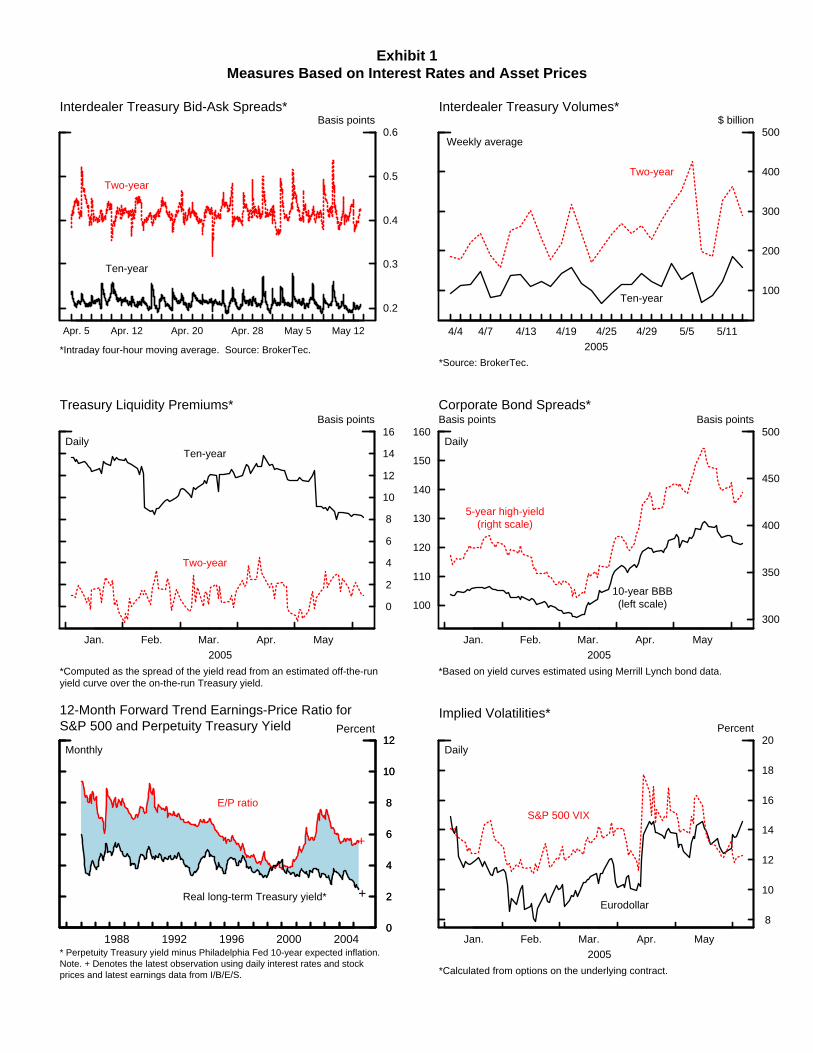
Exhibit 1Measures Based on Interest Rates and Asset Prices

Apr. 5 Apr. 12 Apr. 20 Apr. 28 May 5 May 12

0.2

0.3

0.4

0.5

0.6 Basis points

Two-year

Ten-year

*Intraday four-hour moving average. Source: BrokerTec.

Interdealer Treasury Bid-Ask Spreads*

4/4 4/7 4/13 4/19 4/25 4/29 5/5 5/112005

100

200

300

400

500$ billion

Interdealer Treasury Volumes*

Weekly average

Two-year

Ten-year

*Source: BrokerTec.

Jan. Feb. Mar. Apr. May2005

0

2

4

6

8

10

12

14

16Basis points

Treasury Liquidity Premiums*

Daily

Two-year

Ten-year

*Computed as the spread of the yield read from an estimated off-the-runyield curve over the on-the-run Treasury yield.

100

110

120

130

140

150

160


300

350

400

450

500Basis points Basis pointsCorporate Bond Spreads*

Daily

5-year high-yield(right scale)

10-year BBB(left scale)

*Based on yield curves estimated using Merrill Lynch bond data.

0

2

4

6

8

10

12

1988 1992 1996 2000 2004

E/P ratio

Real long-term Treasury yield*

+

+

* Perpetuity Treasury yield minus Philadelphia Fed 10-year expected inflation.Note. + Denotes the latest observation using daily interest rates and stock prices and latest earnings data from I/B/E/S.

12-Month Forward Trend Earnings-Price Ratio forS&P 500 and Perpetuity Treasury Yield

Monthly

Percent

0

2

4

6

8

10

12


8

10

12

14

16

18

20Percent

Implied Volatilities*

Daily

S&P 500 VIX

Eurodollar

*Calculated from options on the underlying contract.

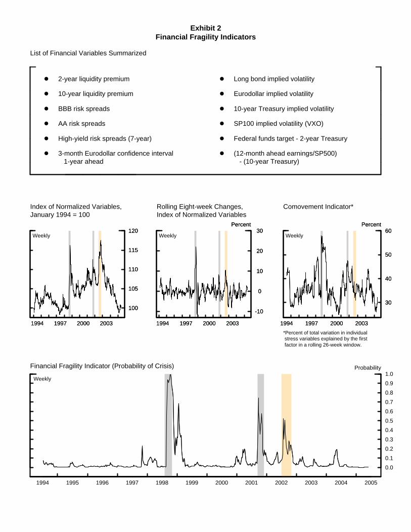
Exhibit 2Financial Fragility Indicators

List of Financial Variables Summarized

●

●

●

●

●

●

●

●

●

●

●

●

2-year liquidity premium

10-year liquidity premium

BBB risk spreads

AA risk spreads

High-yield risk spreads (7-year)

3-month Eurodollar confidence interval 1-year ahead

Long bond implied volatility

Eurodollar implied volatility

10-year Treasury implied volatility

SP100 implied volatility (VXO)

Federal funds target - 2-year Treasury

(12-month ahead earnings/SP500) - (10-year Treasury)

1994 1997 2000 2003

100

105

110

115

120

Index of Normalized Variables,January 1994 = 100

Weekly

1994 1997 2000 2003

100

105

110

115

120

1994 1997 2000 2003

-10

0

10

20

30Percent

Rolling Eight-week Changes,Index of Normalized Variables

Weekly

1994 1997 2000 2003

-10

0

10

20

30Percent

1994 1997 2000 2003

30

40

50

60Percent

Comovement Indicator*

Weekly

*Percent of total variation in individual stress variables explained by the first factor in a rolling 26-week window.

1994 1997 2000 2003

30

40

50

60Percent

1994 1995 1996 1997 1998 1999 2000 2001 2002 2003 2004 2005

0.0

0.1

0.2

0.3

0.4

0.5

0.6

0.7

0.8

0.9

1.0ProbabilityFinancial Fragility Indicator (Probability of Crisis)

Weekly

19940.0

Probability

Exhibit 3Mortgage Market Indicators

Jan. May Sept. Jan. May Sept. Jan. May2003 2004 2005

2.0

2.5

3.0

3.5

4.0

4.5

5.0Years

Mortgage Duration*

Weekly

*Based on a large pool of fixed-rate mortgages included in outstandingmortgage-backed securities. Source: Merrill Lynch.


0.0

0.5

1.0

1.5

2.0

2.5

3.0

3.5$ trillion

Amount of 10-Year Equivalent Securities Needed toMaintain a Constant Portfolio Duration*

Weekly

*Staff estimate based on a duration target of 4.5 years.

0

20

40

60

80

100Percent

Thirty-year fixed-rate mortgage rate

Percentage of Economically RefinanceableMortgages*

4 .0 5 .0 6 .0 7 .0 8 .0 9 .0

5.62

*Cumulative percentage of fixed-rate mortgages included in Fannie Mae’s,Freddie Mac’s, and Ginnie Mae’s outstanding MBS that would beeconomically refinanceable for any given mortgage rate. Source: Bloomberg.


-2.0

-1.5

-1.0

-0.5

0.0Years

Mortgage Convexity*

Weekly

*Based on a large pool of fixed-rate mortgages included in outstandingmortgage-backed securities. Source: Merrill Lynch.


2000

4000

6000

8000

10000

120003/16/90=100

MBA Refinancing Index*

Weekly

*Source: MBA.


1.1

1.2

1.3

1.4

1.5

1.6

ConvexityDuration GapRefinancing Index

Amplification of Interest Rate Shocks According toThree Hedging Measures*

Weekly

*Based on Perli and Sack (2003)

Exhibit 4Measures of Conditions of Individual Institutions

July Sept. Nov. Jan. Mar. May2004 2005

200

400

600

800

1000

1200Basis points

Credit Default Swap Spreads*

Daily

*Source: Markit.

General Motors

Ford

CCC

B

0

2

4

6

8

10

12

1 3 5 7 10 15 20 30

Percent

0

2

4

6

8

10

12

1 3 5 7 10 15 20 30

Percent

0

2

4

6

8

10

12

1 3 5 7 10 15 20 30

Percent

●

●

●

● ● ● ● ● ●

●

●

●

● ●● ● ● ●

● ● ● ● ● ● ● ● ●

Risk-Neutral Probabilities of Default*

Maturity

General Motors

Ford

Wal-Mart

*As of May 31, 2005. Source: MFST staff calculations.


40

50

60

70

80

90

100Basis points

Investment-grade CDS Indexes*

Daily

*Source: Markit.

Traded

Liability-weighted


200

300

400

500

600Basis points

High-yield CDS Indexes*

Daily

*Source: Markit.

Traded

Liability-weighted

2001 2002 2003 2004

0

2

4

6

8

10Percent

General Motors’ One-year Probabilities of Default*

Monthly

Actual (KMV)

Risk-neutral(from CDS)

*Source: Moody’s KMV and MFST staff calculations.

0

50

100

150

200

250

2001 2002 2003 2004

0

100

200

300

400

500

600

700Basis points Basis points

Corporate Risk Premium*

MonthlySpeculative-grade

(right scale)

Investment-grade(left scale)

*Source: MFST staff calculations.

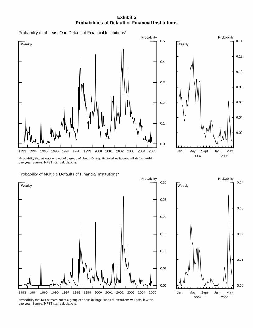
Exhibit 5Probabilities of Default of Financial Institutions

1993 1994 1995 1996 1997 1998 1999 2000 2001 2002 2003 2004 2005

0.0

0.1

0.2

0.3

0.4

0.5Probability

Probability of at Least One Default of Financial Institutions*

Weekly

*Probability that at least one out of a group of about 40 large financial institutions will default withinone year. Source: MFST staff calculations.

Jan. May Sept. Jan. May2004 2005

0.02

0.04

0.06

0.08

0.10

0.12

0.14Probability

Weekly

1993 1994 1995 1996 1997 1998 1999 2000 2001 2002 2003 2004 2005

0.00

0.05

0.10

0.15

0.20

0.25

0.30Probability

Probability of Multiple Defaults of Financial Institutions*

Weekly

*Probability that two or more out of a group of about 40 large financial institutions will default withinone year. Source: MFST staff calculations.

Jan. May Sept. Jan. May2004 2005

0.00

0.01

0.02

0.03

0.04Probability

Weekly

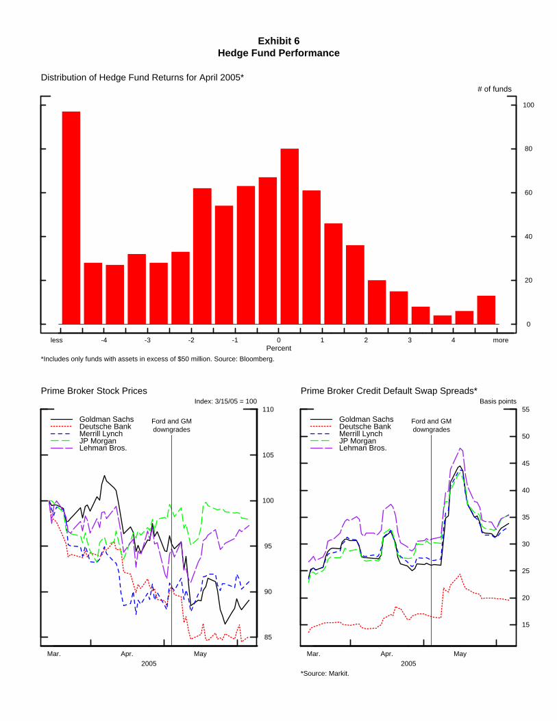
Exhibit 6Hedge Fund Performance

Mar. Apr. May2005

85

90

95

100

105

110Index: 3/15/05 = 100

Goldman SachsDeutsche BankMerrill LynchJP MorganLehman Bros.

Prime Broker Stock Prices

Ford and GMdowngrades

Mar. Apr. May2005

15

20

25

30

35

40

45

50

55Basis points

Goldman SachsDeutsche BankMerrill LynchJP MorganLehman Bros.

Prime Broker Credit Default Swap Spreads*


*Source: Markit.

0

20

40

60

80

100

# of funds

-4 -3 -2 -1 0 1 2 3 4 moreless

Distribution of Hedge Fund Returns for April 2005*

*Includes only funds with assets in excess of $50 million. Source: Bloomberg.

Percent

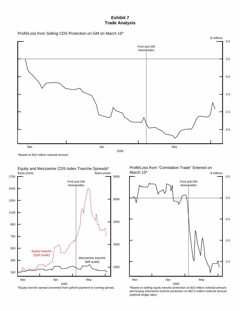
Exhibit 7Trade Analysis

Mar. Apr. May2005

-2.0

-1.5

-1.0

-0.5

0.0

0.5$ millions

Profit/Loss from Selling CDS Protection on GM on March 15*


*Based on $10 million notional amount.

150

350

550

750

950

1150

1350

1550

1750

Mar. Apr. May2005

1500

2000

2500

3000

3500Basis points Basis pointsEquity and Mezzanine CDS Index Tranche Spreads*

*Equity tranche spread converted from upfront payment to running spread.


Mezzanine tranche(left scale)

Equity tranche(right scale)

Mar. Apr. May2005

-1.5

-1.0

-0.5

0.0

0.5$ millions

Profit/Loss from "Correlation Trade" Entered onMarch 15*


*Based on selling equity tranche protection on $10 million notional amountand buying mezzanine tranche protection on $42.5 million notional amount(optimal hedge ratio).

Documents

Selected Indicators of Financial Stability · Selected Indicators of Financial Stability ... assisting in the formulation and implementation of policies regarding Reserve Banks' credit