SELECTED CHAPTERS OF CORPORATE FINANCE AND RISK …

SELECTED CHAPTERS OF CORPORATE

FINANCE AND RISK MANAGEMENT

Edited by Barbara Dömötör and Kata Váradi

2019

SELECTED CHAPTERS OF CORPORATE

FINANCE AND RISK MANAGEMENT

Edited by: Barbara Dömötör and Kata Váradi

Corvinus University of Budapest, Department of Finance

Reviewed by: Péter Csóka, Barbara Dömötör, Gergely Fazakas, Péter Juhász,

Emilia Németh-Durkó, Dóra Gréta Petróczy, Melinda Szodorai, Kata Váradi,

György Walter

Budapest, 2019

© Edina Berlinger, Péter Csóka, Barbara Dömötör, Gergely Fazakas, Péter

Juhász, Krisztina Megyeri, Helena Naffa, Emilia Németh-Durkó, Dóra Gréta

Petróczy, Melinda Szodorai, Kata Váradi, György Walter

The studies serve exclusively academic purposes. Download is free. In case of using any part

of the book for teaching or research, please follow citation rules.

The book can be downloaded from: http://unipub.lib.uni-corvinus.hu/4282/

ISBN 978-963-503-799-5

Published by: Corvinus University of Budapest, 2019

http://unipub.lib.uni-corvinus.hu/

http://unipub.lib.uni-corvinus.hu/4282/

3

Preface

This book was prepared for the Finance Master program of the Corvinus

University of Budapest started in the academic year 2019/2020. The book

consists of two main parts, the first part deals with corporate finance and

financing issues, while the second part covers risk management and liquidity

management in financial markets.

The cases in this book highly build on the knowledge base of the master’s

program curriculum, therefore, it is imperative for students to familiarize

themselves with the basic notions first, before starting to solve the exercises. If

you experience any knowledge gaps, then refer to the regular textbooks before

solving the cases.

In several cases, the related regulations should also be read in conjunction with

the case in order to be able to understand and solve the exercises. This highlights

the ever increasing relevance of regulation in the finance industry.

Apart from the knowledge of the financial notions, and related regulations,

students should also be skilled in using spreadsheets, since several cases cannot

be solved without it.

We recommend the book both to master’s students in Finance and to

practitioners as well.

The Editors

4

Content

Preface ................................................................................................................ 3

Content ............................................................................................................... 4

Part I: Corporate Finance ................................................................................... 7

1. Financial calculations: Annuity (Gergely Fazakas) ................................ 7

Aim and theoretical background ................................................................. 7

Case ............................................................................................................. 8

Questions ..................................................................................................... 8

References ................................................................................................. 12

2. Buying a flat in Budapest (Gergely Fazakas) ........................................ 13

Aim of the case ......................................................................................... 13

Case ........................................................................................................... 13

Questions ................................................................................................... 16

References ................................................................................................. 16

3. How to finance: buying a flat in Budapest (Gergely Fazakas).............. 18

Aim of the case ......................................................................................... 18

Questions ................................................................................................... 21

References ................................................................................................. 21

4. Acquisition financing – DAC Corporation (György Walter) ................ 22

Aim and theoretical background - Structured finance .............................. 22

Case – DAC Kft. ....................................................................................... 25

Questions ................................................................................................... 44

References ................................................................................................. 45

5. Different drivers of an M&A transaction – Buying Wine&Dine (Péter

Juhász) .......................................................................................................... 46

Aim and theoretical background ............................................................... 46

The purchase of Wine&Dine restaurant ................................................... 50

Questions ................................................................................................... 53

References ................................................................................................. 53

6. Global capital budgeting (Edina Berlinger) .......................................... 54


5

Case ........................................................................................................... 56

Questions ................................................................................................... 59

References ................................................................................................. 59

7. Modeling lending in corporate finance under moral hazard (Péter Csóka)

............................................................................................................... 61


Case ........................................................................................................... 62

Questions ................................................................................................... 63

References ................................................................................................. 64

8. Using real options for real estates (Dóra Gréta Petróczy – Emilia Németh-

Durkó) ........................................................................................................... 66


Real options .............................................................................................. 66

Why invest in the real estate market? ....................................................... 67

How to value real estates? ......................................................................... 69

The case .................................................................................................... 70

Questions ................................................................................................... 73

References ................................................................................................. 73

9. Real option pricing with Monte-Carlo simulation (Edina Berlinger –

Krisztina Megyeri) ........................................................................................ 76


Case ........................................................................................................... 78

Questions ................................................................................................... 79

References ................................................................................................. 79

10. Optimal capital structure (Edina Berlinger – Helena Naffa) ............. 81


Case ........................................................................................................... 83

References ................................................................................................. 84

Part II: Risk Management ................................................................................ 86

11. Measuring market risk of equity portfolios (Barbara Dömötör) ....... 86


Regulation ................................................................................................. 88

Useful formulas ......................................................................................... 88

6

Case ........................................................................................................... 89

References ................................................................................................. 91

12. Expected Shortfall: a critique using the CAPM (Péter Csóka).......... 93


Questions ................................................................................................... 95

References ................................................................................................. 95

13. Market liquidity – New asset allocation at LiqWi Ltd. (Kata Váradi) ..

........................................................................................................... 97


Case ........................................................................................................... 99

Questions ................................................................................................. 101

References ............................................................................................... 101

14. AsiaXchange CCP – Initial margin calculation for central

counterparties (Kata Váradi)....................................................................... 103

Aim and theoretical background ............................................................. 103

Case ......................................................................................................... 104

Questions ................................................................................................. 106

References ............................................................................................... 106

15. Managing risks and getting under the central counterparty’s skin

(Melinda Szodorai) ..................................................................................... 109


Case ......................................................................................................... 111

Questions ................................................................................................. 113

References ............................................................................................... 113

16. Credit risk measuring (Barbara Dömötör) ....................................... 115


Regulation ............................................................................................... 117

Case ......................................................................................................... 119

Questions / exercises ............................................................................... 121

References ............................................................................................... 121

7

Part I: Corporate Finance

1. FINANCIAL CALCULATIONS: ANNUITY

Gergely Fazakas

Aim and theoretical background

Annuities, special cash flow-series are interesting problems not only in the

corporates’ life but in everyday life as well. Possible calculations, estimations

of the different parameters need analysis in detail.

Annuities and perpetuities have two meanings in English.

The first meaning is a mathematical problem, referring a special cash flow

series. If it is an annuity, then we have constant cash flow at regular intervals

for a fixed time period; if it is a perpetuity, then we have a cash flow at regular

intervals forever. (See e.g. Ross et al. 2006, pp. 157–166.) In both cases the

default scenario has the following assumptions:

flat yield curve;

same cash amount at each period (there is no growth rate);

cash elements coming yearly;

the first cash flow coming at the end of the first period.

The second meaning is a financial tool – we can call it an art of investment or

from the other point of view as an insurance tool. The two parties – the investor

and the other party, who gets the annuity – agree in a given cash flow-series,

paid by the investor until the death of the other partner. The deposit behind this

transfer or the compensation for this payment is the other partner’s real estate –

usually his/her home, he/she lives in.

So, this contract has an essential actuarial point of view. The key problems are:

What is the fair value of the real estate?

How long will the owner of the real estate live?

Of course, there is some additional problem to answer and to solve:

- Will be any growth rate in the cash flow-series? (E.g. inflation-adjusted)

- Is there any immediate cash flow to be paid?

8

- When can the investor use the real estate – immediately, just after the

death of the other partner, or there are some other options?

- Is there only one person, who gets this annuity, or more – usually couples

– and the investor has to finance this investment until both deaths?

This case study fits into one double lesson. Going through a complete problem

we can analyze the whole theme. There is quite a short preface, just a short

definition of the problem – and then there is a long list of questions. The ranking

of these questions make the structure of the lesson – I believe, that using this

guideline would make an interesting frame, and students could be interested in

the popping up new problems. For this reason, I will not give all the parameters

in the beginning – we can make a debate in the group, and then the group will

end up in a democratic solution (with the help of the instructor) – or at least I

hope so.

Case

We would make an annuity contract with uncle Steve – we will pay him a yearly

sum until his death in exchange to his flat. Uncle Steve has a two-bedroom, 60

m2 flat in Budapest, on Pest side, in a small block of flats. This house was built

ten years ago, standing on a 400 square-yard property. You cannot build any

bigger real estate on that property – according to the construction rules of the

district. The founding charter of the house declares, that the owners of the other

flats do not have any preliminary right to buy other flats in the house. Uncle

Steve has not any heir, he lives alone in his flat, he is 72 years old, and according

to the estimations, he will live an extra 13 years1.

Questions

1. Give an estimation to the value of the flat! What estimation method

would you use for it?

a. Multipliers?

b. Present value method?

c. Options?

d. Substitution – reproduction value?

e. Which estimation method suits for what type of investor?

1 Another case study regarding the usage of a real estate can be found in Jáki (2017)

9

f. Is there any need to make a positive or negative correction in the

values?

According to professional estimations the value of the flat is 40 million forints.

2. Is there any consequence of the founding charter about preliminary

rights?

3. Why is it important, that he lives alone?

4. What is the required rate of return on this field?

a. What is the required rate of return renting out a flat?

b. Is there any other element generating extra profit / extra rate of

return?

The required rate of return on this segment of real estate investments is 9%

annually. (The inflation rate is 3%.)

5. Who will use the flat in the next 13 years?

a. Uncle Steve will live in it.

b. Uncle Steve will move into old people’s home.

c. We will pay a certain amount to Uncle Steve at the beginning,

and he should move.

d. How could you built these assumptions into the calculations?

i. Would you build the effects into the value of the house?

ii. Would you change the required rate of return?

We can use the house from the starting date of the contract, and Uncle Steve

will move out to his relatives in the countryside, to the village called Hevesalso.

6. OK – so what would be our estimation for value of the flat and for the

required rate of return?

7. In the contract we would declare, that we will pay a constant annual

amount to Uncle Steve until his death. (So as to make an easy

calculation, we will pay just once a year.) Overall we will count with a

13-element annuity. Let’s get this factor (For example from an annuity-

table). What is the fair yearly sum to pay?

8. Uncle Steve would take our offer. What happens, if we paid back the

whole remaining debt? How much should we pay?

a. What is the fair calculation using future-value method? (Paying

interest + principal)

10

i. Which cash flow element has priority – interest or

principal?

ii. What does this priority mean from legal point of view and

from mathematical point of view?

b. What is the fair calculation using present value-method?

9. Using annuities – what does our formula assume? We pay at the

beginning of each period, at the end or in the middle of the period? Does

it suit for our contract? Does it suit for renting flats?

10. Uncle Steve asks us to pay at the beginning of each year. We should

recalculate the fair yearly payment.

a. Let’s use a 12-element annuity!

b. Let’s shift our original annuity!

c. What is the ratio between the original payment and the new

payment? (In percentage.) And what is the ratio between the 12-

element annuity factor and the 13-element annuity factor?

11. Now we are able to calculate the fair monthly payment! We would divide

the present yearly payment into 12 monthly payment.

12. What is the monthly required rate of return?

13. What is the fair monthly payment?

a. If we pay at the end of each month.

b. If we pay at the beginning of each month.

14. Let’s turn back to the construction with the yearly payments. Let’s

assume, that Uncle Steve would take payments at the end of each year.

We will pay 13 times, at the end of each year. What would be the first

payment, if Uncle Steve asked inflation-adjusted payments? We assume

a flat inflation rate at 3%.

a. Let’s use the real rate of required return.

b. Let’s use the formula of growing annuity.

c. Is there any difference between the two results? (Did we use a

fair real rate of return in our calculation?)

15. We will change our mind. We would pay a constant 5 million per year.

How long should Uncle Steve live to get a fair contract? (Use excel or

annuity table – but do calculate the annuity-factor first!)

11

16. Our next idea is to pay even less. Our offer is only 3.5 million forints per

year. How long should live Uncle Steve to get a fair contact? How can

we check our result with the help of payment-structure of the annuities

(interest + principal)?

17. What is the value the annuity-factors go to in the column of 9%?

18. Taking this limit, what yearly payment is the theoretical minimum

making a fair contract?

19. Uncle Steve takes our 5 million forints offer. We are quite happy,

because we should pay a lower sum than the fair value. Great deal!

(Uncle Steve will live for 13 years, in average). What is the internal rate

of return of the contract? Is it higher or lower than 9%?

20. Let’s explain the result and its relation to 9%!

a. Is it an active or passive transaction?

b. Is it investment or debt taking – financing problem?

c. What do the words „investment” and „debt taking” mean

i. for a lawyer;

ii. for a book-keeper;

iii. for an investor?

21. How do conventional cash flow series look like?

Let’s use the following, very simple problems.

A. You invest 1 million forints today, and will get 1.1 million forints in

one year.

B. You will take a debt: 1 million forints today, and you will have to

pay back 1.1 million forints in one year.

22. How does the function of present value and net present value of a

conventional cash flow series look like? (the independent variable is the

required rate of return)

a. In the case of debt taking? At what rates of return do we have

positive and negative NPV-s? At what rate of return do we have

the internal rate of return.

b. In the case of investments? At what rates of return do we have

positive and negative NPV-s? What is the internal rate of return?

12

References

Most of the financial textbooks deals with annuities, like:

Brealey, R.A., Myers, S.C. & Allen, F. (2017). Principles of Corporate Finance,

12th ed, McGraw Hill, 2017, 2nd Chapter.

van Horne, J.C. & Wachowicz jr., J.M. (1991). Fundamental of Financial

Management, Prentice Halls, New Jersey, 8th ed., 1991, pp. 51-60.

Jáki, E. (2017). Kertvárosi ház hasznosításához készített megvalósíthatósági

tanulmány, in Jáki, E. (2017). Üzleti terv pénzügyi vonatkozásai. Befektetések

és Vállalati Pénzügy Tanszék Alapítványa, Budapest pp. 18-30.

Ross, S.A., Westerfield, R.W. & Jordan, B.D. (2006). Corporate Finance;

Fundamentals. McGraw-Hill Irwin, 2nd edition., pp. 157 – 166.

Száz, J. (1999). Tőzsdei opciók vételre és eladásra, Budapest 1999, pp. 45-46.

13

2. BUYING A FLAT IN BUDAPEST

Gergely Fazakas

Aim of the case

Now, in 2019 we are very sorry, that we hadn’t bought a flat five years ago –

we just had not thought about it, or we could not have financed it. The financial

crisis seriously affected the prices of flats in Budapest: the prices were

stagnating between 2009 and 2014, or even they were descending by 10-20%.

(E.g. see the flat price index from the National Bank of Hungary)

On the other hand, prices of flats in Budapest between 2014 and 2019 had been

more, than doubled. Were we losing all the chances for a good investment?

Would not have been a better idea to buy a flat previously using a bank loan?

That is true, that meanwhile the currency-crisis only a few investors could have

risked taking additional bank loans. (In those area banks were cautious as well,

they would have landed loans only under very strict conditions.) But now we

are in 2019, and thanks to the boom, we do have enough money to invest. We

would like to buy a flat, and get a permanent income renting it out2.

Case

The chosen real estate is in the 9th district of Budapest, it is a 50 m2 small flat

with two bedrooms. The house has very good transport possibilities: both metro

line no. 3 and the tram 4-6 is very closed. There are 3 universities nearby.

The flat would be ideal for singles, young couples, or even for couples with one

or two small children. After a short discussion, you could get the flat for a

reasonable 35 million forints. The house was built 35 years ago, so not new –

but both the house and the flat itself is in good condition. A normal painting

(400.000 forints) would be needed anyway.

We would analyse different concepts, but one thing is essential: we are risk

averted, so we will declare and pay all the taxes (15%) linked to renting out.

Painting out is urgent – we will be ready with it within a month. Meanwhile, we

will be able to find a tenant as well. (The cost of advertisement will be

somewhere between 5000 and 10.000 forints, the cost of our time included.) We

2 Another case of utilization of a house can be found in Jáki (2017).

14

are planning to rent it out for 15 years – our older son will be eighteen by that

time, and after a greater reconstruction he would live in.

Utilization

Let’s start with utilization. We have two ideas.

a. We would make a long-term renting contract. We will get a suitable

tenant within a month. The monthly fee would be 150.000 forints,

unfurnished. Gas, electricity, water will be paid by the tenant – all

those contracts will run under his name. We assume, that within the

15 years renting period there will be no greater reconstruction

needed.

b. Our second option is Airbnb – as far as the flat is quite closed to the

inner city. We assume that we will have guests 180 days a year, and

can take four guests. The first day of each transaction would cost

18.000 forints, each additional day would cost 14.000 forints. At this

case, we should buy furniture and household appliances. At the

arrivals of the guests, we should clean it up and welcome them.

Our plan for renting out through Airbnb as follows:

Table 1. The Airbnb renting out plan

Month Days

rented out

Number of

reservations

January 11 4

February 8 3

March 13 5

April 15 5

May 18 6

June 20 6

July 22 6

August 22 6

September 16 5

October 9 3

November 8 3

December 18 6

Sum 180 58

15

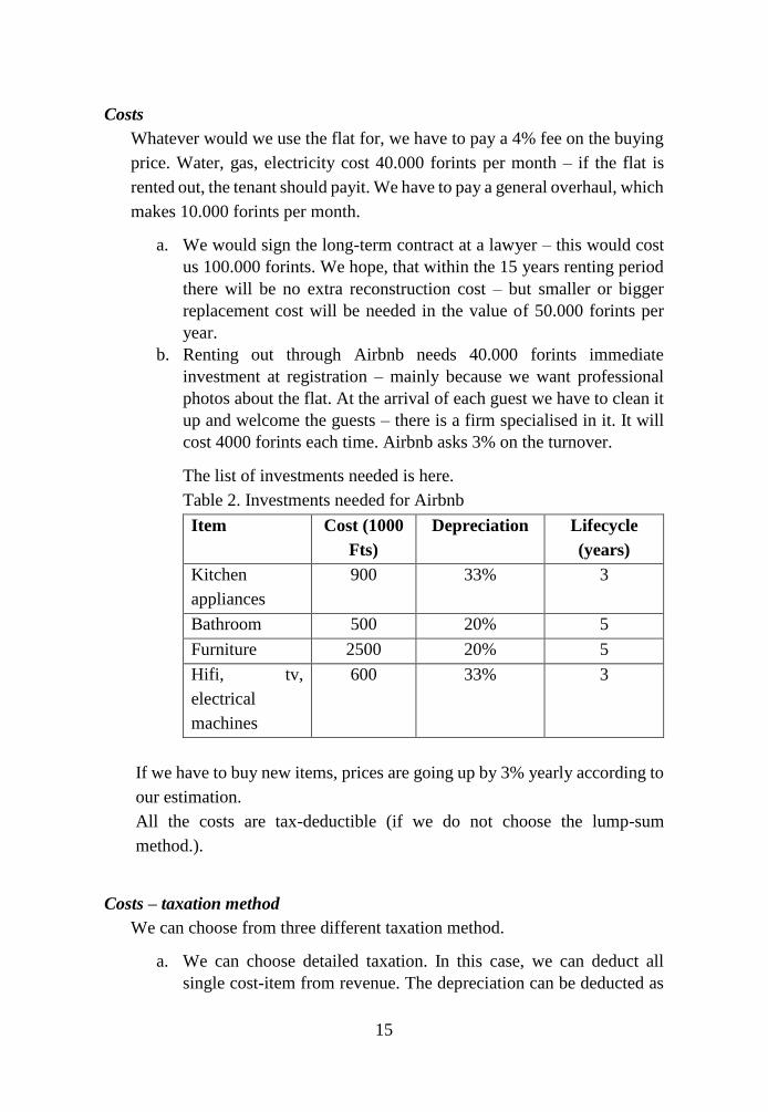
Costs

Whatever would we use the flat for, we have to pay a 4% fee on the buying

price. Water, gas, electricity cost 40.000 forints per month – if the flat is

rented out, the tenant should payit. We have to pay a general overhaul, which

makes 10.000 forints per month.

a. We would sign the long-term contract at a lawyer – this would cost

us 100.000 forints. We hope, that within the 15 years renting period

there will be no extra reconstruction cost – but smaller or bigger

replacement cost will be needed in the value of 50.000 forints per

year.

b. Renting out through Airbnb needs 40.000 forints immediate

investment at registration – mainly because we want professional

photos about the flat. At the arrival of each guest we have to clean it

up and welcome the guests – there is a firm specialised in it. It will

cost 4000 forints each time. Airbnb asks 3% on the turnover.

The list of investments needed is here.

Table 2. Investments needed for Airbnb

Item Cost (1000

Fts)

Depreciation Lifecycle

(years)

Kitchen

appliances

900 33% 3

Bathroom 500 20% 5

Furniture 2500 20% 5

Hifi, tv,

electrical

machines

600 33% 3

If we have to buy new items, prices are going up by 3% yearly according to

our estimation.

All the costs are tax-deductible (if we do not choose the lump-sum

method.).

Costs – taxation method

We can choose from three different taxation method.

a. We can choose detailed taxation. In this case, we can deduct all

single cost-item from revenue. The depreciation can be deducted as

16

well –this is 2% on the flat and 14,5% on the furniture and

appliances. Choosing this possibility we have to ask a book-keeper

to help us – this would cost 10.000 forints monthly.

b. We can also choose the “lump sum” method. In this case, 10% of the

revenue can be the total cost, so as 90% of the revenue will be taxed.

No extra costs can be deducted from the revenue. (NAV, 2017)

c. Taxes on rooms. There is a special rule: if the rooms are rented out a

maximum 180 days a year, you can choose this method. This case

the yearly tax is 38.000 forints per room. (So 76.000 forints for our

flat – as far as we can rent it out the whole in one.) You have to pay

it at the beginning of each fiscal year.

Terminal value

At year 15 we would give the flat to our older son. At this stage, the flat will

be in medium condition. On the real estate market, we presume a 3% yearly

inflation rate.

The required rate of return

The required rate of return on renting out a flat is 8%.

Using Airbnb is riskier because we have to face with country-risk, exchange

rate risk and higher operative risk as well. In that case, we can use a 10%

rate of return.

Questions

1. Can you give an estimation for the future cash-flow for the next 15 years

month-by- month?

2. What are the NPV and the Internal rate of return of each scenario? Which

possibility gives us the highest values?

References



és Vállalati Pénzügy Tanszék Alapítványa, Budapest, pp. 18-30.

17

MNB (2019). Flat price indices. https://www.mnb.hu/letoltes/mnb-

lakasarindex-eng.pdf

Downloaded: 02.07.2019.

NAV (2017). Public information about taxation on paying hospitality.

https://en.nav.gov.hu/taxation/taxinfo/rent_of_real_estates.html


https://www.mnb.hu/letoltes/mnb-lakasarindex-eng.pdf

https://www.mnb.hu/letoltes/mnb-lakasarindex-eng.pdf

18

3. HOW TO FINANCE: BUYING A FLAT IN BUDAPEST

Gergely Fazakas

Aim of the case

We are now in 2019. On the Hungarian market, flat-prices have been growing

by roughly 20% annually in the last 5 years. Although it can be a risky

investment, we have decided to buy a flat and rent it out on a long run.

According to some experts, the prices are on the top just now, and a recession

can be expected within 1-2 years. We cannot finance such a business ourselves,

but our brother-in-law (who has a wide portfolio of different real estates) is

ready to take part in our project.

This case is dealing with different financing methods.

The chosen real estate is in the Inner district, the 6th district of Budapest. It is a

60 m2 small flat with two bedrooms. The house is in a walking distance from

the old underground (called Kisföldalatti) line and from the trams on Grand

Boulevard (in Hungarian Nagykörút).

We could get it for 40 million forints – this price is quite favourable, although

the flat is not even in the “medium condition”. Our reconstruction expert

estimates the costs of the reconstruction as 8 million forints – he can start the

works immediately and within two months they can finish the whole project.

Although there are several possibilities to finance the project, one thing is

essential: we will be the only owner, we ourselves will pay all the costs, and all

the taxes linked to the flat will be declared and paid.

The renting-out is planned for 10 years – that is the maximum time horizon we

can make financing plans and our brother-in-law would like to exit by that time.

1. Utilization

We have agreed with our brother-in-law to make a long-term renting contract.

The flat is suitable for diplomats, young managers or young couples. We believe

that for 200.000 forints renting fee (unfurnished) we would easily find a reliable

tenant (within a month).

19

We would ask a 2-month deposit as well. Gas, electricity, water will be paid by

the tenant – all those contracts will run under his name. We assume that within

the 10 years renting period there will be no greater reconstruction needed.

2. Costs

Buying a flat we have to pay a 4% fee on the buying price. Water, gas, electricity

cost 40.000 forints per month. We have to pay a general overhaul, which makes

10.000 forints per month. We would sign the long-term contract at a lawyer –

this equals one-moth renting fee, so 200.000 forints. We hope, that within the

10 years renting period there will be no extra reconstruction cost.

All the costs are tax-deductible – if we choose the detailed cost-deduction tax

method.

3. Costs – taxation method

We can choose from different taxation methods. We could have chosen the

detailed taxation method, but our brother-in-law hates the meticulous

administrative tasks – so we will use the “lump-sum” method. In this method,

90% of the revenue is the tax base, and no real costs are tax deductible (NAV,

2017; Ado, 2018).

4. Financing

We have two ideas to finance the buying price and all the extra costs.

a. If we finance the whole project ourselves, we would need the

help of our brother-in-law. He is ready to pay 50% of all costs

and investments, and he would ask 50% of all the incomes after

tax. At year 10 he would exit, so we will have to buy the 50%

ownership.

b. We would take a bank-loan. The loan would be 10-years long,

payment due monthly. The interest rate would be 6% yearly (on

a linear basis). The cost of the loan 100.000 forints, immediately

payable (e.g. cost of the notary).

The only collateral behind the loan is the flat itself. The bank can

give us a loan up to 50% of the value of the flat. Although

sometimes asking a loan is quite a long and difficult process,

thanks to our connections and experience we could get in within

20

some days. About more details of mortgage and other retail loans

and the loan approval process see: Walter (2016) or Jáki (2018).

5. “Baby-bond”– state aid for young couples with children

There is a state aid – a special loan – for young couples with children. We have

a son, so we can get this special loan. We can get 10 million forints as a loan for

10 years – paying back monthly as an annuity. The 1st children means, we do

not have to pay any interest. We will have our 2nd child at the end of the 2nd year.

The 2nd child means that 30% of the original amount of the loan will be wiped

out. Asking a Baby-bond” is not so easy, the time and administration would cost

50.000 forints for us.

The Baby-bond can be combined with the “normal” bank-loans as well.

6. Terminal value

At year 10 we will think about the usage of the flat. It can happen, that we would

buy out our brother-in-law, but also a possible scenario to sell the flat together.

At this stage the flat will be in medium condition. On the real estate market we

presume a 4% yearly inflation rate. Nowadays flats in medium condition are

priced 10% lower, than average. A newly renovated flat would cost 10% higher

than the average. We presume, that there will be a 4% inflation on reconstruction

costs as well.

7. The required rate of return

Renting out a flat is not riskless at all. The long term risk-free rate of return is

4%, and we will calculate a 6% market premium.

To live in a flat is an inferior need, so the rate of return on renting out will be

below the market rate of return, just 8%.

If we are taking a bank-loan, we assume that the loan is risk-free. The bank had

so many and o strict collaterals and restrictive rules, that they will not risk

anything. For simplicity we suppose that 50% of the investment will be debt-

financed.

21

Questions

1. What is the future cash flow for the next 10 years month by month?

2. What are the NPV and the Internal rate of return of each scenario? Which

possibility gives us the highest values?

References

Ado (2018). Public information about taxation on paying hospitality.

https://ado.hu/ado/a-lakaskiadasbol-szarmazo-jovedelem-adozasa/


Jelzalog (2019). About the state aid for young couples.

https://jelzalog.com/csok/ Downloaded: 09.08.2019.

Jáki. E. (2018) Finanszírozási elképzelések pénzügyi modellezése: Miskolc

Nyomda hosszú távú pénzügyi tervezés. In: Jáki, E. (2018). Pénzügyi

kimutatások, gyakorlati pénzügyi modellezés; Budapesti Corvinus Egyetem, pp.

55-73.

NAV (2017). Public information about taxation on paying hospitality.



Walter, Gy. (2016). Kereskedelmi banki ismeretek, Alinea.

https://ado.hu/ado/a-lakaskiadasbol-szarmazo-jovedelem-adozasa/

https://jelzalog.com/csok/


22

4. ACQUISITION FINANCING – DAC CORPORATION

György Walter

Aim and theoretical background - Structured finance3

The aim of the following case is

to analyze the different risk aspects of acquisition financing;

to understand the business concept and model of IT companies;

to carry through and acquisition finance approval process, and

to make a decision on its possible structure, terms and conditions.

The term of „structured finance” is difficult to define. In some definitions, it is

a transaction where the risk analysis and financing decisions are not based on

the balance sheet and the assets of the company but on the forecasted cash-flow.

It is a product where the transaction and its financing must be structured tailor-

made to meet all requirements and expectations of the stakeholders and

participants. These transactions usually involve high leverage, high risk, longer

and more complex preparation, a thorough due diligence process, analysis of the

cash-flow capability, and a more complex contractual and legal structure. Based

on the literature, the most important groups of structured finance are as follows

(Jobst, 2005, pp. 19–21.):

High leverage financing (like acquisition financing)

Project financing (like real estate development, energy projects, etc.)

Securitization

Structured trade finance

On the corporate level most of the transactions belong to the first two groups, to

high leverage financing and project financing. The sale of these products is not

only typical in commercial banking but merges with other services of

investment banks like advisory, syndication, origination. Therefore, investment

banks and corporate finance firms are also active participants of such

3 See Walter (2014b)

23

transactions joint by technical and other special advisors, legal firms, auditors,

etc.

Transaction types that belong to the group of high leverage financing are as

follows:

Acquisition financing

Leveraged Recapitalisation (Recap)

Leveraged asset-based finance

Among these groups, acquisition financing is possibly the most frequent

transaction. It is about buying a whole (or substantial part of a) company,

therefore the volume of the transaction is high. It usually involves debt financing

resulting high leverage at the end.4 The acquisition loan and its repayment

schedule appear as a new, considerable burden on the company that is added to

all former debts of the company. The high leverage must be paid back based on

a tight cash flow plan.

Acquisitions usually include complex structures with many participants where

different types of conflicts of interests arise. There is a potential new investor

accompanied by a bank who both face high risk. To mitigate these risks other

players also step in, whose tasks, interests and conflicts must be also managed

and coordinated. The potential participants in a transaction are:

New owners, investors, the buyers;

Former owners, the sellers;

Banks and other financing institutions (factor firms, leasing companies)

Mezzanine funds

Legal experts, legal firms;

Technical, tax, environmental, PR and other advisors, experts;

Corporate finance advisor of the seller;

Corporate finance advisor of the buyer;

Auditors

Authorities

…

4 There could be a connection between acquisition financing and IPOs too, see Szabó and Szűcs

(2014).

24

Transaction structures could be various, tailor-made to the certain deal. The

figure below shows one of the simplest and commonly used financing and

contractual structures of an acquisition.

Structure of an acquisition financing

Source: Walter (2014b)

The provision of the loan is prior to the change of ownership. Therefore, it is

difficult to solve – from the structural point of view – how the acquisition loan

“is put inside” the target company and how it is linked to the cash-flow, to the

assets and the collaterals of the operating company. In most cases, a special

company is needed (an SPV, that is a „special purpose vehicle”), which takes

up the loan, gets the equity sponsorship of the new owners, pays the purchase

price, and receives the stake, the ownership (shares, equity) of the target

company. The SPV is usually a non-operating company, it holds the equity of

the target company, acts as an owner, receives the necessary cash-flow from the

company to be able to provide the debt service of the acquisition loan. This

structure implies several technical, tax, accounting, and legal issues and

problems, like: how and based on what cash-flows are flowing from one

company to the other; how collaterals and guarantees can secure a loan of

another company. To solve these problems target company and SPV sometimes

merge, though it usually takes several months to close up such a merge process.

All sponsors, especially financial investors, try to avoid any recourse financing

and intend to limit their liabilities to the volume of the equity sponsorship.

However, industrial investors are more likely to accept a recourse financing and

25

shows more flexibility to back the new acquisition loan with its balance sheet,

cash-flow, or with a corporate guarantee. In the case of MBO transactions,

personal guarantees of the new owners, as a proof of commitment, are also an

accepted practice and it usually plays an important role in the success of the

deal.

Case – DAC Kft.

Dominika took the document from the table. She blinked at the monitor. It was

the 17th of September 2007. Monday, 9.13 a.m. She was the head of the

Structured Finance Desk and has had quite a lot to do nowadays. First, the Bank

Headquarter had several questions concerning the real estate crises that got

surprisingly bigger and bigger on the market. Filling the reports to the

headquarter consumed a lot of energy and time. On the other hand, there were

many transactions in the pipeline and she wanted to do all of them. But only if

they are feasible, of course. The current deal described in the document was a

typical, small, local acquisition loan, where almost the whole documentation

was ready. Most of the business and cash-flow scenarios were done, the credit

application was almost complete, only a few parts were missing, these were all

highlighted with yellow.

She carefully read through the whole credit application.5

5 For definitions and terms of credit application see Walter (2014a).

26

Credit application

CREDIT DECISION REQUIRED

BY:

Transaction Name:

DAC Deal

Transaction Details:

MBO of a significant actor of the document

archiving, document management and workflow

management market

Underwriting

Requirement:

A. Senior long-term loan HUF 128.8

million

B. Credit line HUF 10.0

million

C. Guarantee HUF 5.0

million

Available documents: Business plan for 2007-2012

Annual reports of DAC, 2001-2006

Balance sheet and P&L of the first half of 2007

Information Memorandum

List of references

Description of the activity and the products

Integrator contract signed with TELCO1 and with

PRINTCO Rt.

Exemplars of delivery contracts, support

contracts and software update contracts

Drafts of contracts to be signed with

TRASPORTCO

Introduction – Transaction Background

DAC Kft. is a market leader in the Hungarian document archiving/management

and workflow management segment. Current owners of DAC Kft. have decided

to offer the Company for sale to a strategic buyer. One of the present owners,

Mr. Balázs Vezér (as a preemptive right) would like to get 100% ownership of

the Company. He intends to finance the deal at leverage, and requested a long-

term EUR loan to finance the transaction. Furthermore, he also intends to get a

27

credit line in order to match the financing of temporary given orders and

contracts.

Transaction Structure

Current structure

The Company’s ownership is currently shared by three Hungarian private

individuals, namely Mr. Béla Owner with a quota of 40%, Mr. Balázs Owner

with a quota of 40% and Mr. Balázs Vezér with a quota of 20%. Mr. Vezér is

also a member of the management.

New structure

According to the plans of Mr. Vezér, DAC Kft. becomes a single-owned

company. The total purchase price is HUF 184 million, and Mr. Vezér intends

to finance 70% of the purchase price at leverage. The total amount of loan

provision is equivalent to HUF 128.8 million, currently EUR 511 thousand in

single draw-down. Consequently, about half of company value is financed at

leverage.

Mr. Vezér intends to purchase the remaining 80% of the Company’s ownership

through a project company. Current owners of DAC will sell their quota to the

project company of Mr. Vezér through a foreigner project company. After the

transaction (planned to take place until the end of 2007) the project company

and DAC merge, so that DAC gets the loan.

Company Overview

DAC Kft.

DAC was established by three Hungarian private individuals (Mr. Béla Owner,

Mr. Balázs Owner and Mr. Balázs Vezér) in 2000. Two of the founders, Béla

and Balázs Owner have been involved in the optical and image recognition

sector since the early 90’s, and are founders of several IT companies. Mr. Vezér

is the CEO of the Company since its foundation. He graduated at the Technical

University of Budapest, and started to work as a developer for several

companies during his university years. He also worked for FAC, a company

owned by Mr. Béla and Balázs Owner, of which DAC grew out.

DAC Kft. is active in the document archiving/management and workflow

management sector. In the first year after establishment, DAC was providing

an archiving and document management product for small and medium size

companies. Shortly after the beginning, the Company’s focus changed to

28

provide software products for large enterprises. Currently, DAC produces and

sells document archiving and management software product under the brand

name CLEVERARCHI, and does the integration of the software with

customers’ Enterprise Resource Planning systems. DAC also performs the

customization, regular product updates and support over the life of the contract.

DAC’s proprietary office automation solution has been sold to over 100

companies in Hungary. This product (the software CLEVERARCHI Digital

Office) was designed to perform complex document archiving and management

functions for medium and large size organizations. Suiting the needs of

customers, DAC provides efficient, quick and secure filing, archiving and

management of physical and electronic documents. It enables not only the

storing but also the quick retrieval of mailing and other confidential data. The

distinctive feature of CLEVERARCHI in this field is its rapidity and reliability

(e.g. retrieval is performed in seconds in case of order of magnitude for millions

too).

The main functions the software has are the following:

1. Filing/registry: The software fully replaces traditional filing/registry

methods. It can handle registries of arbitrary number, and makes the

managing of transmitter, posting and other register books unnecessary.

Retrieval of documents according to different aspects is feasible.

2. Archiving: CLEVERARCHI can store and manage scanned paper-based

and electronic documents. Pictures of documents archived and data are easy

to be retrieved and to be on view.

3. Workflow support: The software supports the execution of everyday work

and multi-stage workflow effectively, and makes them easy to schedule and

control. CLEVERARCHI delegates the tasks to the appropriate teams, does

the deadline monitoring and warning of users, performs reports and does the

fill-in of blank forms.

Subsequently the main user functions of CLEVERARCHI are: input of paper-

based documents by scanning; fax and mail server in order to integrate internal

and external flow of information (also able to register and archive incoming

faxes and mails automatically); managing appendices (registry numbers,

addresses, remarks, comments etc.); recognition and assignment of printed

29

characters, digits and bar-codes to the documents registered; grouping of

documents; multi-aspect retrieval of documents, data export into different file

formats; search (in scanned documents as well); picture viewer (picture of

documents stored appears on the screen); reports, statistics in arbitrary structure

(e.g. on the efficiency of a team etc.); deadline watching and warnings

(CLEVERARCHI Message, e-mail or SMS); distribution and signing of

documents; recording and tracking the storage location of documents archived.

The software also offers DAC inistration functions, such as the customization

of documents view, maintenance of users and the authority system; tuning of

capacity and efficiency of the system, performance monitoring.

Besides software development and sale, the Company also provides peripheral

hardware tools needed, such as scanners, bar-code readers, bar-code printers,

and provides service connected. Special hardware tools the Company provides

for its customers are:

1. CamScan: This equipment enables the input, restore and archiving of

documents and data sheets (e.g. CVs, personal data sheets, identity cards

etc.) in the computer, supplied with color photos as well. The equipment

contains a black-and-white scanner (in order to read sheets), a color camera

(in order to record photos/pictures) and an Optical Character Recognition

device (which recognises printed characters). The technical oddity of this

equipment is the parallel use of a black-and-white scanner and a color

camera, which makes the functioning of CamScan faster and more

economical than equipment using a color scanner.

2. Speedy Reader, Passport Reader: Speedy Reader is an optical data input

tool, which records the postal cheque laid on the target disk and converts it

into a data readable by computers. Passport Reader is a data input tool to be

integrated into computer networks, which can take photos of and read data

in personal documents of different types (passports, identity cards etc.),

performs examination of authenticity and forwards collected data.

3. Gepard File Encryptor USB Key: This is a microcomputer running an

encrypting algorithm, which enables an efficient protection of confidential

data, encoding and decoding files, folders, folder structures.

30

DAC executes the installation, maintenance of hardware tools and training of

users as well.

Further activity of the Company includes the software package Registauto,

which does the storage, evaluation and transmission of data on sciatic prosthesis

surgery, collected in accordance with standard medical aspects.

DAC also developed a polling system used in elections (e.g. ethnic autonomous

elections in 1999, 2006).

DAC executes (1) system DAC inistration, (2) the operation, supervision and

maintenance of central computer pool, (3) network management and (4)

software development within the frameworks of an outsourcing activity as well.

Management/Employees

DAC has a total number of 19 core employees (including management). The

Company has 13 additional employees, who provide outsourcing services for

Telco2. More than 70% of employees are designing engineers or computer

professionals.

The management team consists of five people, namely: Mr. Balázs Vezér, CEO;

Mr. GS., Head of Sales and Marketing; Mr. T. V.; Head of Product

Development; Mr. P. P., Head of Implementation; and Mr. B.G., Head of

Support. Each member of management has a qualification in the field of

technology and long-term experience on the planning and implementation of

large systems. Majority of managers emerged from DAC’s staff. Mr. Vezér

plans no changes in management structure in the future.

Core markets and competition – Competitive landscape

Market trends

The market of so-called content and document management systems is to grow

dynamically not only in Hungary, but in the EU as well. Founded on a survey

on content and document management6 in some European countries (UK,

Benelux, France, Germany and Scandinavia) made by Rethink Research

Associates, penetration in the developed Europe is still quite low. An average

penetration of 33% was calculated from the survey, however, only Germany

6 Enterprise content management consists of the following: (1) document management; (2) web

content management; (3) digital asset management; (4) records management and (5) workgroup

collaboration. DAC doesn’t deal with web content management, so that the findings of the

survey can be applied only restrained.

31

(37%) and France (29%) can take pride in around 30% penetration figures.

Much lower share of the companies in the rest of the countries/regions examined

have such systems in use (17% of Benelux and 7% of Scandinavians). Of the

companies examined that currently have no content/document management

system, 60% plan to invest in one in the coming two years, and 48% of the

companies having content management system expect to extend their

installations in the coming two years. The key factors behind their intention are

the clarification of workflow and business processes, the management of digital

assets (e.g. copyrighted works) and the compliance with legislation and

regulation in the US and the eurozone.

Figures above point to the fact that (concerning development differences) the

penetration of content management systems in Hungary is surely deep under the

lowest observed ratio of 7%. The penetration on the target market of DAC is in

addition lower, concerning that the systems examined by the survey cover a

wider range (see in footnote). As a result, the potential for market growth is

much larger in Hungary than in the developed Europe. Regarding the driving

factors, EU regulation and legislation (besides the intention to keep firmer

control of corporate performance and efficiency) is an important motivational

factor in the examined countries.

In Hungary, a low level of function exploitation is a basic characteristic. The

demand for expanding functions is mainly typical of large innovative

companies. Small size enterprises are at an initial stage described by system

establishment and network development, using mainly the e-mailing function.

Medium size enterprises cannot be categorized, either large, or small

enterprises’ features can be applied for them, particularly depending on the

number of sites and client base. However, according to Microsoft Hungary,

medium size enterprises will be the main target in the next 5 to 10 years.

According to DAC’s estimations, the size of large enterprise market amounts to

about 5000 companies. SME sector covers a wider range of companies of over

20 000. The financial size of market is hard to be estimated because of the

existence of orders without tendering, but after DAC’s managers it can be set to

HUF 1-1.5 billion a year.

Customers, partners

The target market of DAC is the large and medium size organizations segment.

In this segment, projects are usually tendered to a select group of companies

active in the document archiving and management field. According to DAC’s

32

management, the Company is invited to the majority of the tenders written by

large customers in Hungary, and has an over 50% win-rate. DAC as vendor of

the document archiving/management technology participates on these tenders

very often in consortium with major IT multinationals. Besides participating at

tenders, sales are carried out through direct approach, or occasionally by

participating on local trade shows.

Further opportunity for acquiring clients is provided by the integrator contract

signed with Telco1 and planned to be signed with SAP and PRINTCO Rt. In the

sense of the contract signed with Telco1 Rt., Telco1 and DAC cooperate to

satisfy adequate needs of 3rd parties. (Essentially Telco1 recommends the

products and services of DAC for its customers, according to DAC’s

management.) This contract has a maturity of one year (signed on 1st June 2007),

and automatically elongates with one year unless abrogated. (See in contractual

review.) The sense of the strategic partnerships planned with SAP and

PRINTCO is the same.

The management also purposes to enter on the document archiving/management

market of foreign countries in the future. The planned cooperation with

PRINTCO would be a determining step in this direction because of PRINTCO’s

extended relations with actors of foreign markets (mainly in former socialist

countries).

The importance of these contracts is to be detected in the decreasing costs of

client acquiring as well. This kind of cooperation makes the pre-sales period

much shorter, DAC has to latch on to client management only at the point of

bidding. (Without integrator contract, pre-sales period can last from 2 months

to 1.5 years, consisting of the addressing of marketing materials, visitation at

reference clients etc.)

Main customers of DAC include major local companies and Hungarian

subsidiaries of multinational firms. Major customers in 2006 were:

Water Co.: revenue EUR 159 000; share 21%;

Dutility: rev. EUR 87 000; share12%;

Telco2: rev. EUR 80 000; share 11%;

Chemco: rev. EUR 78 000; share 11%;

Gasco: rev. EUR 51 000; share 7%;

OILCO: rev. EUR 38 000; share 5%.

Other customers together (Metalco Kft., CarCo Hungária Kft., Bank1 Rt. etc.)

had a 33% share of revenues in 2006.

33

The Company had 35 clients (small and big ones together) in 2006. According

to the experiences so far, 60% of newly acquired small size clients and 100% of

large ones remain in the customer base of DAC. Due to the great potential of

increase in the Hungarian market, the Company plans to duplicate its client base

until 2012. Managers of DAC plan their future acquirement of large clients

based on the analysis of top 50 ranking of companies acting in Hungary. The

number of companies in the top 50 working without document/workflow

management systems is 17.

The pipeline of the company is promising, it shows that the company is

contacting about 40-45 companies in a potential contractual value of HUF 600

million. However only HUF 26 million value of contracts has been signed out

of the list on the date of the application.

Contract types

The contracts DAC signs with its customers can be divided into three main

categories:

one off delivery contracts, which result in a single payment for

customizing, installing and delivering the products;

support contract: general maturity of 1 year, payment depending on

the client (monthly/quarterly/yearly in advance or posteriori);

software update contract: yearly charge to be paid in advance,

maturity generally 1 year.

Almost all large clients and nearly 50% of small clients require support service

– small ones either in the form of indefinite maturity contracts or ad hoc

engagement. Experiences so far show that active customers require support each

year. The average price of support amounts to HUF 0.5 million yearly.

Upgrade is required by active clients who use their systems constantly, and in

each year get their systems upgraded. The mean price of upgrade totals HUF 0,6

million/year.

Besides, DAC signed a contract on outsourcing activity with TELCO2. In

pursuance of this contract, DAC provides service for TELCO2 on site. The main

tasks are: input of subscriber contracts into Contract Management System and

receptionist task performance. In order to perform these tasks, 13 employees of

DAC are at TELCO2’s service, remunerated after working hours accomplished.

34

Competitors

Actors on the Hungarian market can be either suppliers of 3rd party products, or

suppliers of proprietary products. Experience shows that DAC successfully

competes against both types of market players due to the functional features of

its products, good customer references and easy adaptability of its product to the

ERP systems used by its customers. The main competitors of DAC are:

proprietary product suppliers: Montana, IBM, Graphton, Freesoft

and Archico (also supplier of 3rd party products);

3rd party product suppliers: T-Systems, Hewlett Packard, IQ Soft

and Synergon.

Contractual Review

Integrator contract signed by DAC and Telco1 Rt. has a maturity of one year

(signed on 1st June 2007), and automatically elongates with one year unless

abrogated.

Outsourcing contract with TELCO2 is signed without maturity. Abrogation

time is asymmetric: in case of TELCO2’s abrogation, it totals 3 months; in

case of DAC abrogating the contract, abrogation period amounts to 6

months.

Exemplars of delivery contracts, support contracts and software update

contracts are available. Specific terms of each contract depend on the client.

Financing facilities required by DAC

Long-term loan of HUF 128.8 million for financing acquisition of 80% of

DAC.

A credit line of HUF 10 million, in order to finance eventually appearing

working capital needs, available for separate transactions, disbursed on the

basis of individual decisions. Credit line is needed for the import

procurement of hardware tools (the purchase price has to be settled in

advance at the distributor abroad).

DAC’s guarantees at two commercial banks in an amount of nearly HUF 5

million will be taken over by CORPBANK with cash collateral.

35

Suggested Terms and Conditions

Long-term loan

Amount HUF 128.8 million

Facility type / Maturity / 5 years

Denomination HUF

Draw-down Single draw-down.

Repayment even repayment, quarterly

Coupon payment Quarterly, actual/360

Base rate 3 months BUBOR

Margin 1.2 DSCR < 1.5 400 bp

1.5 DSCR < 2.5 350 bp

2.5 DSCR < 3.5 300 bp

3.5 DSCR < 4.5 250 bp

4.5 DSCR 200 bp

Up-front management fee 1%

Covenants Negative pledge, Ownership clause,

Pari passu, Cross default

Fresh long-and short term borrowing

with the consent of the Bank

Senior debt (all other liabilities are

subordinated)

Quarterly financial report

Securities Assignment of sales revenues

Pledge over all fixed and floating

assets, licenses, trademarks

Other conditions Opportunity for pre-repayment

36

Credit line

Amount HUF 10 million

Facility type / Maturity / Revolving

Denomination HUF

Coupon payment Quarterly, actual/360

Base rate Overnight BUBOR

Margin 1.2 DSCR 1.5

300 bp

1.5 DSCR < 2.5 250 bp

2.5 DSCR < 3.5 200 bp

3.5 DSCR 150 bp

Up-front management fee 1%,- flat

Commitment fee 1% p.a.

Guarantee limit

Amount HUF 4.8 million

Facility type / Maturity / Revolving

Denomination HUF

Fee payment Quarterly

Guarantee fee 2 %

Up-front management fee -

Financial Evaluation

Historic performance

DAC’s performance since 2004 has progressed remarkably – showing the

widening of its activity and client base. The net income increased from a loss of

HUF 2.27 million to a gain of over HUF 21 million. Gross margin amounted to

nearly HUF 67 million in 2006, which gives 36% of net revenue (HUF 20

million in 2001 and HUF 48 million in 2002). EBITDA in 2006 totaled HUF 30

million. This year’s figures show a flourishing operation: turnover in the first

half of 2007 (totaling HUF 75 million) indicates a 12% increase related to the

corresponding value in 2006, while EBITDA amounts to nearly HUF 20 million.

These figures don’t truly characterize the Company’s performance, as – due to

37

the sector’s features – major part of sales is always realized in the last quarter

of the year.

The Company has total assets of HUF 106 million, a third of which consists of

fixed assets (value HUF 35 million). The Company has inventories of a minimal

value (HUF 2 million in 2006), which results from the immediate selling of

assets purchased from a 3rd party. Inventories appearing in the balance sheet of

DAC consist of marketing materials, the value of which increases parallel with

net revenue. Customer claims are relatively high due to favorable payment

conditions given to its customers.

DAC doesn’t have any short- or long-term loan. Its liabilities comprise of

prepayments from its customers (HUF 1 million in 2006), trade suppliers (HUF

43 million in 2006) and other short-term liabilities (HUF 8 million in 2006,

including basically tax liabilities). Value of trade suppliers typically increases

parallel with the rise in net revenue.

Projections – Client’s case

HUF 128.8 million (EUR 511 thousand) credit

Maturity 5 years

Interest rate: 11%

Revenue increases significantly

Constant ratio (of 2007) of material type expenditures/revenues

Slight improvement in personal type expenditures/revenues despite

enlarging manpower and wages increasing by 5%

HUF 72 million total CAPEX until 2012 (a conservative projection of yearly

CAPEX HUF 12 million, which is expectedly higher than the real need of

the activity)

Average income from support amounts to HUF 0.25 million/year/ active

client, average revenues from upgrade total HUF 3 million/year/active client

happens every 5 years in average (every 5th client)

Average on-off revenue by new client acquisition is 16 million HUF

Conclusion

In the case of client’s plans coming true, cumulated cash-flow calculated

following debt service is strongly positive. The financing power of the

transaction is especially demonstrated by considering that a conservative

estimation of CAPEX is used for calculation (according to the management, a

38

CAPEX of nearly HUF 4 million is supportable from year 2008).

Accomplishment of repayment and interest payment isn’t endangered in client’s

case.

Projections – Break even

…

Projections – Conservative case

…

SWOT Analysis

Strengths

…

Weaknesses

…

Opportunities

…

Threats

…

39

ROE

The transaction offers to Corpbank an expected pre-tax ROE of 13.14% and a

gross revenue of HUF 6.92 million for 2007.

Amendment

DAC’s client base widened newly by acquiring TRASPORTCO. Negotiations

are proceeding, and the contracts are expected to be signed in the near future.

This deal offers a huge increase in DAC’s revenues, so that the risk of financing

the MBO becomes much lower. Service contracts to be signed ensure monthly

revenues of at least HUF 25 million from 1st January 2008 (earliest maturity on

31st December 2013), so that TRASPORTCO may become the largest customer

of the Company (HUF 25 million/month is the minimum amount that will be

paid by TRASPORTCO, the maximum can reach HUF 37 million/month).

Besides, three other contracts are to be signed:

(1) a supplier contract on the hardware tools needed (in a value of HUF 97.4

million; margin around HUF 30 million);

(2) an auditing contract with a monthly revenue of HUF 3.57 million (the

margin of which totals 100%; earliest maturity on 31st December 2010);

(3) a contract on consultancy until 31st December 2007 in a value of HUF 50

million (which will be performed through subcontractors).

In consequence of this deal, cash-flows streaming from DAC’s operation change

in the following way.

Conclusion

DAC is a significant actor on document archiving/management and workflow

management market. Market penetration of document and workflow

management systems in Hungary is fairly low, so that the Company’s

management forecasts further increase in revenues due to widening client base.

….

Summarised: The main risk of the deal …

Considering risk factors and profitability based and relied on available

information, we ...

40

APPENDIX 1. Acquisition pipeline at DAC Kft. (reflecting latest information)

Client Value eFt

Energyco2 60 000

Bank2 40 000

Energygroup 40 000

Gas3co 40 000

Retailco2 40 000

Cosntructionco 30 000

Transportco 30 000

Zenon 30 000

Airco 25 000

Beerco2 25 000

Energyco5 25 000

Beerco1 20 000

Gasc4co 20 000

Itco 20 000

Pow erco 20 000

Verticon 15 000

Chemco Rt 12 000

Dutility 12 000

Printco 11000

Oillco 10 000

Stateco, Debrecen 10 000

Waterco2 10 000

Retailco1 9 803

ÉVR 8 000

Constr2 7 761

Waterco3 6 700

BBB 5 000

Oilco 4 000

Client1 2 626

Retailco1 2 400

Carco1 2 000

Logictics 2 000

41

APPENDIX 2. A classification of DAC’s activities

The main activities DAC performs in the field of office documentation and

document management are:

developing software for office automation; selling software

CLEVERARCHI Digital Office:

CLEVERARCHI Digital Office Software enables the secure

long-term storage of mailing and confidential data by storing

large amount of paper-based and digital documents, the

software enables to retrieve a file in seconds and to make

workflow monitorable;

the functions CLEVERARCHI provides are: registry,

archiving (paper-based and electronic documents and

identifiers), workflow support (automatic allocation of tasks,

deadline-watching and warnings);

CLEVERARCHI is an integrated client-server software able

to be integrated into existing information systems, and to

work together with mailing, groupwork and control systems;

CLEVERARCHI’s main feature and its most important

differentiating factor to competition are the easy integration

of the software with SAP, Scala and other ERP systems;

distributing software Registauto used for surgery database

management;

operation and distribution of polling systems;

software related services:

(file handling) workflow assessment; development,

integration and installation of workflow management

systems;

training for users and system DACinistrators;

support: hot-line telephone support; on-the-site support;

intervention;

updating;

planning and installing specialized data input units and scanners;

distributing, installing and maintaining peripheral hardware tools:

scanners, bar-code readers and printers, special hardware

developments, CamScan (which enables to input, store and

42

archive documents, data sheets supplied with color photos),

Speedy Reader M70+ (optical data input tool, which records

the postal cheque laid on the target disk and converts it into

a data readable by computers), Passport Reader;

hardware related services:

installation, training, guarantee, warrantee, maintenance;

special services related to handling of documents:

arrangement, rejection, shredding and rehousing of files,

documents;

permanent management of filing-cabinets;

document storing and supplying of data;

internet-based services;

postal services;

selling and manufacturing wrappers for handling documents;

business services:

operation of central computer pool;

network management;

software development;

outsourcing activity (special services): preparing regulation

for file handling; filing-cabinet services; lease-scanning; data

registering.

43

APPENDIX 3. Clients case and financials

avarege annual support revenue/client 250 THUF

average annual upgrade revenue/client 600 THUF

acquisiton one off revenue/ client 16 000 THUF

tax rate 16%

'000 HUF Fact

P&L Statement 2006 2007 2008 2009 2010 2011 2012

Net revenues 188 476 … … … … … …

growth … … … … … …

Telco2 outsourcing revenues 31 054 32 640 34 272 35 986 37 785 39 674 41 658

One-off revenues (client acquisition) 125 000 … … … … … …

Upgrade revenues 23 672 … … … … … …

Support revenues 8 750 … … … … … …

Material type expenditures 118 390 … … … … … …

% of revenue 63% 44% 44% 44% 44% 44% 44%

Personal type expenditures 31 428 … … … … … …

% of revenue 17% 35% 28% 27% 26% 25% 25%

Other revenues 0 0 0 0 0 0 0

Other expenses 8 522 6 284 7 115 8 398 9 164 10 491 11 042

Depreciation 6 967 7 691 8 983 9 888 10 522 10 965 11 276

EBITDA 30 136 … … … … … …

Operational result 23 169 … … … … … …

Net result of financial operation 561 0 0 0 0 0 0

Result of ordinary operation 23 730 … … … … … …

Net extraordinary profit 0 0 0 0 0 0

Pre-tax profit 23 730 … … … … … …

Income taxes 2 381 … … … … … …

After-tax profit 21 349 … … … … … …

Dividend

Balance sheet profit 21 349 … … … … … …

Cash-flow 2007 2008 2009 2010 2011 2012

EBIT … … … … … …

Depreciation 7 691 8 983 9 888 10 522 10 965 11 276

Income tax … … … … … …

Gross Cash-flow … … … … … …

Change in Net Working Capital -5 073 -6 -2 553 1 640 -1 538 4 575

Free Operational Cash-flow (before CAPEX, debt

financing)… … … … … …

CAPEX -12 000 -12 000 -12 000 -12 000 -12 000 -12 000

Free Cash-flow … … … … … …

Change in financial investments 13 850 500 0 0 0 0

Financial Cash-flow 13 850 500 0 0 0 0

Total Cash-flow … … … … … …

Total debt service … … … … … …

Cumulated Cash-flow (after debt service) … … … … … …

ADSCR … … … … … …

Number of active clients 35 43 56 70 86 103 121

Number of clients acquired 7 8 13 14 16 17 18

Planned

44

Questions

Dominika read the credit application. Parts that must be completed or needed a

decision were highlighted with yellow. She looked at the financial model

(Appendix 3) that was also not completed yet, however included the basic

structure. She did not have to do any cash-flow models herself nowadays but

this time she decided to finish it alone. It was not difficult at all. First, she wanted

to check the case of the client and its cash-flow. Based on that she wanted to

“play” a little bit with the value drivers; she was curious, how the break-even

and a conservative scenario look like.

She completed the application with these scenarios. She carefully looked and

commented on the term sheet. SWOT analysis was also not completed. She

hated SWOT, but this time she found it useful to understand the risk factors. So,

she completed the SWOT as well. By the time she has finished her job, she had

a firm opinion about the deal. She noted some sentences in the conclusion part

of the application. (She did not consider the 10. point of „Amendment” yet as

she wanted to discuss it with the relationship manager.)

3 months 12 months 13 months 14 months 15 months 9 months

Interest rate 11% 11% 11% 11% 11% 11%

total debt 128 800

interest … … … … … …

repayment … … … … … …

remaining principle 128 800 … … … … … …

credit line outstanding 10 000 10 000 10 000 10 000 10 000 10 000 10 000

Debt service … … … … … …

up front fee …

Blance sheet (MHUF) 2006 2007

Cash 3 4

Acc. Receivables 40 65

Inventories 2 2

Current assets 45 71

Fixed Assets 35 35

Assets 80 106

Acc. Payables 23 44

Otehr short term liab. 7 8

DEBT 0 0

Equity 50 55

Liabilities 80 106

45

She finished her work. She called her colleague who was responsible for the

deal to discuss her findings and conclusions with him. She knew that they had a

lot to discuss.

References

Jobst, A. A. (2005). What is structured finance? Working Paper, September

Szabó, A. & Szűcs, B.A. (2014). Acquisition-driven IPOs - Theory and

Evidence in Central and Eastern Europe, Public Finance Quarterly 2014/1, pp.

94-108

Walter, Gy. (2014a). Sztenderd kereskedelmi banki hiteltermékek.

Vállalatfinanszírozás a gyakorlatban. Alinea Kiadó, Budapest

Walter, Gy. (2014b). Strukturált finanszírozás. Vállalatfinanszírozás a

gyakorlatban. Alinea Kiadó, Budapest

46

5. DIFFERENT DRIVERS OF AN M&A TRANSACTION –

BUYING WINE&DINE

Péter Juhász, PhD, CFA


This case aims not only at reviewing motivations for selling and buying firms

but also to identify different types of possible synergies. The case offers an

opportunity for modelling the bargaining process and understanding its link with

the valuation performed earlier. A unique trait of the case is that it even

illustrates the appearance of asynergies and requires students to address those.

The words mergers and acquisition (M&As) may refer to several kinds of

transactions. (Figure 1) If a company acquires another firm, we categorise the

transaction further as (1) horizontal (buying a competitor from the same

business), (2) vertical (purchasing a firm at a different stage of the supplier

chain, e.g. your supplier or buyer) or (3) conglomerate merger (the activity of

the other entity is unrelated to ours). (Brealey et al. 2011, pp. 792-793.)

We may find several reasons why the owners of a company would be willing to

participate in an M&A transaction either as a buyer or a seller. Seller may need

to liquidate some of their investments to start a new project, could need cash,

may turn old, or be unable to overlook their inherited company. Divorce is also

a classic motive for selling a private firm.

On the buyer side, the will to increase cash flow, decrease the risk of operation

or need of invested capital is entirely in line with the shareholder value

paradigm. However, it seems that there are many other reasons too. Based on an

extensive literature review, Nguyen et al. (2012) state that besides the will of

creating shareholder value, managers tend to support M&As to increase the

organisation they lead for their interest (e.g. compensation, career, fame, hubris)

or to make it more dependent on their own skills and knowledge. The term

market timing refers to the practice where the management of an overvalued

firm uses the shares of their company to pay for another firm that is less

overvalued. By doing so, they try to take profit of the pricing anomaly and

protect themselves against takeovers but may end up purchasing companies

even at inflated prices. It is also common that several different motives act

together as drivers for an M&A transaction.

47

Based on the shareholder value concept, only transactions that create value for

both the seller and the buyer are economically justified. We may achieve this if

both the acquisition premium (seller) and the value created for the acquirer are

positive. These quantities are to calculate as follows.

Figure 1 Classification of acquisitions

Source: Damodaran, 2012, pp. 703.

Value Created for Seller = Acquisition Premium = Selling price – Value for

Seller (1)

Another firm

Tender

offer

Target firm continues to exist, but as a

private business. It is usually

accomplished with a tender offer.

A firm can be

acquired by

Acquisition

of assets

Buyout Its own managers

and outside

investors

Target firm and acquiring firm

combine

to become new firm; stockholder

approval needed from both firms.

Target firm becomes part of

acquiring firm; stockholder

approval needed from both firms.

Consolidation

Merger

Target firm continues to exist as

long

as there are dissident stockholders

holding out. Successful tender

offers

ultimately become mergers. No

shareholder approval is needed for

a tender offer. Approval needed

from both firms.

Target firm remains as a shell

company,

but its assets are transferred to the

acquiring firm. Ultimately, target firm

is liquidated.

48

Value Created for Acquirer = Stand-Alone Value of Target for Buyer +

Value of Performance Improvements in both

Firms – Selling price (2)

To track down the amount of value created, we have to quantify the added value

of the M&A, the so-called synergy that could be partly passed over to the seller

by paying a premium. The synergy is quantified as shown next.

Synergy = ValueforBuyerTogether – ValueforBuyerAcquiring firm –

ValueforBuyerFirm taken over (3)

Note that synergy is the difference between the joint and the stand-alone values

for the same owner. To realize some synergy, we need to have at least two

companies.

Theoretically, an M&A could even pay off if synergy is zero or negative. (A

negative synergy is called asynergy.) To understand this, we have to understand

why one would pay more a firm than the current market value (or value for the

seller in case of a non-listed company). We may list three reasons.

(1) The price for which the firm (equity) can be taken over is less than realistic.

If the market is not efficient (shares are under-priced) or the seller is under some

financial, regulatory, or other pressure, we may get a good deal.

(2) In case the buyer has better market connections, more advanced know-how,

higher bargaining power, or some other competitive advantage, it is possible

that by simply changing the way the company sold operated, the value of the

target firm will rise.

(3) There could be positive effects that are to realize only if owning to specific

companies. If a company purchases its supplier, they may not only cut back on

operational risk but also optimize inventory levels and product development

process. Should a firm purchase its competitor, its bargaining power both on the

selling and buying side will increase, while they may save costs by centralizing

some parallel activities. We call this effect synergy.

In the case of listed firms and liquid markets, synergies are the most likely

motivators for a takeover as it is infrequent that we may earn profit from option

(1) or (2). Undervaluation is usually present for a short period and current

owners, unless not in need of money, tend to wait for better times instead of

selling off their shares. Besides, these companies are far too transparent to allow

poor management to act over a more extended period. However, in the case of

49

private firms, it is not rare to find majority owners under pressure due to

financial need or health issues or lacking adequate knowledge to identify

management shortfalls.

Although we know this, there is still a vast number of researches proving that

most of the transactions create positive value for the sellers but a negative one

for the buyers. (Koller et al. 2010, pp. 448-451.) This value destruction could be

explained by the buyers being too optimistic about future improvements, both

considering the total amount and time resource need of realization. Empirical

research found that strong acquirers (above average profitability and growth),

low premium payment, and being the sole bidder (no price war) increases the

likelihood of creating value for the buyer.

We should not underestimate the importance of this method of shareholder value

creation. It is not that firms just spent extra money not needed for their operation

on these transactions; instead, in some cases, a key motivation for attracting new

shareholder capital and organising IPOs is to finance M&As (Szabó and Szűcs,

2014).

As we may see, it is vital to predicting the value of future improvements

(synergies) as precisely as possible. Damodaran (2012, pp. 707-708.) separates

two main types of synergies. (I) Operating synergies include (1) economies of

scale, (2) higher pricing power, (3) combination of different functional (e.g.

marketing, manufacturing) strengths, and (4) higher growth in new or existing

markets. (II) Financial synergy covers (5) access to excess cash to use if for

financing good projects of the other company, (6) increased debt capacity, and

(7) tax benefits.

We may also categorize synergies based on the way those influence the

collective value of the firms. (Figure 2) Some synergies are (Type 1) added to

the sum of the former values. When an office building is not needed anymore

and could be sold, the income can be seen as a one-time effect. These items are

the easiest to deal with during a valuation process.

Other synergic effects would (Type 2) create a value proportional to the joint

value of the two firms. If productivity would improve thanks to the know-how

acquired from the other firm, or cross-sales would boost income, the synergy is

proportional to the value of the enhanced entity. These items may create a very

different amount of value for different acquirers.

50

Figure 2 Value effects of different synergies

Merged

firm

without

synergies

𝑉𝐵𝑒𝑓𝑜𝑟𝑒 =𝐹𝐶𝐹𝐹𝐵𝑒𝑓𝑜𝑟𝑒

(𝑊𝐴𝐶𝐶𝐵𝑒𝑓𝑜𝑟𝑒 − 𝑔𝐵𝑒𝑓𝑜𝑟𝑒)

Merged

firm

with

synergies

𝑉𝐴𝑓𝑡𝑒𝑟

=(𝐹𝐶𝐹𝐹𝐵𝑒𝑓𝑜𝑟𝑒 + 𝑆𝑦𝑛𝑒𝑟𝑔𝑦𝑇𝑦𝑝𝑒 2)

(𝑊𝐴𝐶𝐶𝐵𝑒𝑓𝑜𝑟𝑒 − 𝑆𝑦𝑛𝑒𝑟𝑔𝑦𝑇𝑦𝑝𝑒 3) − (𝑔𝐵𝑒𝑓𝑜𝑟𝑒 + 𝑆𝑦𝑛𝑒𝑟𝑔𝑦𝑇𝑦𝑝𝑒 3)

+𝑆𝑦𝑛𝑒𝑟𝑔𝑦𝑇𝑦𝑝𝑒 1

Finally, there are synergy elements (Type 3) the value effect of which depends

on other factors or synergic effects. For example, if considering a growing-

perpetuity-like operation, the value effect of a 1 percentage point of increase in

long term growth due to the use of a brand name accessed through an M&A

could be very different both in monetary and percentage terms depending on the

long-term cost of capital that might again be affected by some increased debt

capacity thanks to the transaction. Measuring the effect of these synergic

elements could be extremely challenging in a real-life situation.

Due to these different effects, we can rarely separate the total synergy into

addable elements. The sum of individual synergy effects is usually less than the

total effect. So, a failure to realise some planned cost synergies may reduce the

value effect of a growth synergy achieved even if that is in line with the

predictions.

The purchase of Wine&Dine restaurant

It is December of 2019. The Hotel DreamWell is located near to the famous spa

of Heviz, Hungary that heals and eases various types of musculoskeletal

diseases. The hotel specialised itself on serving elderly arriving mainly from

Germany, Austria and other western countries who provide a relatively high

continuous booking rate. During the recent years, the number of these guests

has slightly decreased as due to the improving living conditions, health care

services and more health-conscious living style followed there are fewer people

aged 50-60 who suffer from illnesses that the spa may cure. Many competitors

compensated this by attracting more travellers from eastern countries, mainly

51

Russia. Instead of that, DreamWell increased its marketing spending in the

EU15 countries to compensate for this trend. Under these conditions, preserving

the excellent connection with travel organisers and guest returning each year

become particularly important.

Just next to the hotel, a restaurant called Wine&Dine operates that offers not

only traditional Hungarian food but also various healthy dishes to stay

competitive. In the neighbourhood, there are various other places offering meals

of various quality and price level. Still, due to the very similar pricing policies

followed, the restaurant provides solid profitability. The firm expects a ROIC

rate of 15 percent in 2020 along with a sales of 300 million HUF. Other details

of their business plan are presented in Table 1.

Table 1. The current business plan of Wine&Dine

2020 2021 2022

Terminal

value

period

Sales growth 6.00% 5.00% 4.00%

EBIT/Sales 21.00% 20.00% 20.00% 20.00%

Corporate tax rate 9.00% 9.00% 9.00% 9.00%

RONIC 14.50% 14.00% 14.00%

D/V 30.00% 30.00% 30.00% 30.00%

Operative cost of capital

for the industry (rA) 14.00% 14.00% 14.00% 14.00%

Cost of foreign capital (rD) 5.00% 6.00% 6.00% 7.00%

At the end of 2019, János Kovács, the CEO of DreamWell comes to the idea

that they could cut on costs if their guests would be served by the Dine&Wine.

The main issue is that while guests require the hotels to offer some in-house

dining opportunity but is very rare that they really would use this service.

Instead, they prefer to walk in the town and try a different restaurant each

evening. However, guests from other hotels never enter DreamWell for to get a

meal. Thus, setting up or buying their restaurant that also receives guests from

the street.

There could be various advantages gained from taking over Wine&Dine.

Thanks to the better soundproofing, the firm could host various night events

without disturbing the sleep of the hotel guests. In addition, buying the

52

restaurant would make the whole current kitchen area redundant. Most of the

kitchen equipment (current book value: 5 million HUF) could be immediately

sold for 10 million HUF. The kitchen area could be transformed into a wellness

centre generating an FCFF of 4.2 million HUF at an annual growth rate of 4

percent. The setup would require an investment of 50 million HUF, the

unleveraged cost of capital for the industry is 12 percent.

Currently, the hotel expects an FCFF of 120 million HUF for 2020. Thanks to

the planned transformation, due to the better restaurant service and the hosting

of more events, the top management expects that the predicted 3 percent growth

may climb to 4 percent for there consecutive years (2020-2022) per year

otherwise the perpetuity-like pattern of the operation remains unchanged.

The operative cost of capital for running a hotel is assumed to stay fixed at 14

percent, the leverage (D/V) stays at 35 percent, the current 10 percent corporate

tax rate will be stable, while the required rate on foreign capital stagnates at 5

percent level. After 2022, the growth of FCFF will be 3 percent.

The CFO of DreamWell believes that thanks to his great connection with some

local bank managers, the hotel could get a debt financing for Wine&Dine up to

35 percent of the total firm value. Due to the centralised marketing efforts, the

current growth rate of the restaurant might be boosted to 8 percent for the next

three years. (After that period, the growth would return to the currently expected

4 percent per year level.) During the same period, RONIC could be enhanced to

15 percent by taking profit of the great supplier connections of DreamWell.

Once approached by DreamWell, the owner-manager of Wine&Dine received

the idea of the takeover cautiously. At the second meeting, he presented his

plans on how to change the current operation of the restaurant. Recently the

number of tourists with Slavic background boosted, he explains. These people

are in their 40s, and their cultural background is quite different. Thus, they have

a strong demand for going out, but the city has not too much to offer. After his

plans, Wine&Dine should turn into a kind of night club that presents an erotic

show two-three times per night after 10 p.m. on a small stage.

Based on his estimations, the transformation will cost 12 million HUF (spent

and capitalized with a useful life of 8 years by the end of the year) and will raise

the EBIT/Sales ratio to 21 percent without any further additional investments

compared to the former plans. The growth rate after 2022 would remain at 5

percent.

The hotel management is scared. As this new image of Wine&Dine would be

utterly inconsistent with the kind of guests DreamWell currently serves, the

53

FCFF of the hotel might fall by 10 percent immediately due to the shock (other

value drivers remain unchanged). The board decides to act immediately to insure

a smooth takeover at a fair price.

You are hired to help them as a consultant. Based on your prior experience the

transaction costs (lawyers, consultants, due diligence, banking fee) for the seller

could amount to 3 million HUF, while that of the buyer may reach 6 million

HUF.

Questions

1. Identify the possible drivers for each party to take part in the planned

M&A transaction.

2. What would be the lowest acceptable (reservation) price for the seller?

3. What would be the maximum price the buyer would be ready to pay?

4. What other aspects and information should the parties consider before

entering the transaction?

References

Brealey, R.A., Allen, F., & Myers, S.C. (2011). Principles of corporate finance.

New York : McGraw-Hill/Irwin.

Damodaran, A. (2012). Investment valuation: Tools and techniques for

determining the value of any asset. Hoboken: Wiley.

Koller, T. Goedhart, M., & Wessels, D. (2010). Valuation: Measuring and

managing the value of companies. Hoboken: Wiley.

Nguyen, H.T., Yung, K., & Sun, Q. (2012). Motives for Mergers and

Acquisitions: Ex-Post Market Evidence from the US. Journal of Business

Finance & Accounting, 39(9/10), pp. 1357–1375.

https://doi.org/10.1111/jbfa.12000

Szabó A. & Szűcs B.Á. (2014). Acquisition-driven IPOs - Theory and Evidence

in Central and Eastern Europe, Public Finance Quarterly, (1), pp. 94-108.

https://doi.org/10.1111/jbfa.12000

54

6. GLOBAL CAPITAL BUDGETING

Edina Berlinger


The aim of this case study is to confront students with the problem of capital

budgeting in a multicurrency environment. Students are supposed to know

basics of project valuation and the Capital Asset Pricing Model (CAPM). Now,

the exercise is to apply these principles for an investor thinking globally and

having investment opportunities in different countries.

If we have to decide whether a project is worth to invest or not, it is the net

present value which is the safest tool. If NPV is positive, it is a good project, if

it is negative, it is a bad project, Arnold (2010). (Internal rate of return IRR can

give the same results if done correctly, however, it can be misleading in some

situations.) If there are capital or capacity constraints, so it is impossible to

realize all attractive projects right now, then it is the profitability value index

(𝑁𝑃𝑉/𝐶0) which helps ranking (Brealey and Myers, 2003, Jáki, 2004).

When calculating net present values (NPV), we define a basis currency called

“home currency” which is the unit of accounting for the given investor. Cash-

flows should be converted into the home currency with the help of spot or

futures exchange rates. Basically, we have two approaches (Brealey and Myers,

2003):

a) First, we calculate the present value of foreign cash-flows with the

help of foreign currency denominated expected returns, then convert

the present value to the home currency with the help of the spot

exchange rate.

b) First, we convert future foreign cash-flows to the home currency

with the help of the corresponding expected future exchange rates,

then calculate their present values using home currency denominated

expected returns.

Doing correctly, the two approaches give the same result, but the second one

may be processed easier. Expected future exchange rates can be calculated by

the formula:

55

𝐸(𝑆𝑡) = 𝑆0 (1 + 𝑟𝑡

ℎ𝑜𝑚𝑒

(1 + 𝑟𝑡𝑓𝑜𝑟𝑒𝑖𝑔𝑛

)(1 + 𝑐𝑟𝑝))

𝑡

where 𝑆0 is the spot exchange rate (the price of one unit of foreign currency

expressed in the home currency), 𝐸(𝑆𝑡) is the expected exchange rate for time

t, 𝑟𝑡ℎ𝑜𝑚𝑒 is the expected rate of return in home currency for time t, 𝑟𝑡

𝑓𝑜𝑟𝑒𝑖𝑔𝑛 is

its counterparty in foreign currency, and crp is the country risk premium of the

foreign currency relative to the home currency.

Note that the uncovered interest rate parity does not hold necessarily, as some

currencies are riskier than others from the investors’ perspective, hence country

risk premia are not always zero. Dömötör (2019) analyzed the fulfillment of the

uncovered interest rate parity in the Hungarian market. In principle, we could

hedge future cash-flows on the futures markets (i.e. convert them in advance at

predetermined rates), however, the problem is that we have only estimations for

the future cash-flows, but we cannot be sure of these quantities in advance.

Expected rates of return are usually estimated using the classical pricing formula

of the CAPM:

𝑟𝑖 = 𝑟𝑓 + 𝛽𝑖(𝑟𝑚 − 𝑟𝑓)

where 𝑟𝑖 is the expected rate of return of the i-th project, 𝑟𝑓 is the risk-free rate,

𝛽𝑖 is the beta of the i-th project, and 𝑟𝑚 is the expected rate of return of the

market portfolio (Brealey and Myers, 2003, Bodie et al. 2011). (Of course, all

these parameters can be different for different times t. For the assumptions

behind the CAPM models see eg. Fazakas, 2018)

When implementing CAPM, the most important questions to answer are:

- What is the risk-free rate? As the investor calculates everything

in the home currency, the risk-free rate is the corresponding

treasury bill rate in the home currency.

- What is the market portfolio? As the investor thinks globally, the

market portfolio should be represented by a global portfolio (e.g.

MSCI global index), however, the expected return should be

estimated by converting returns into the home currency first. The

investor considers all returns in the home currency; therefore,

56

correlations should also be calculated between returns expressed

in the home currency.

Note that using classical CAPM in this multiperiod and multicurrency context

is not correct theoretically, firstly because CAPM is a one-period model, and

secondly because CAPM assumes that all investors have the same basis

currency and the same risk-free rate. The correct method would be to use a

multiperiod version of the zero-beta CAPM (Black, 1972, Bodie et al. 2011)

where the risk-free rate is replaced by the zero-beta pair of the market portfolio.

In this case study, however, as most practitioners do, we set aside these problems

and use the classical CAPM being aware of its limitations. Naffa (2009) shows

empirically how asset pricing anomalies may occur.

Betas can be estimated (i) directly from the covariance matrix; (ii) indirectly

from betas of the competitors (Brealey and Myers, 2003). Results are not

necessarily the same but should be close to each other. In case (ii), we have to

be careful with equity betas as they cannot be taken from the competitors due to

the differences in financial leverages. In contrast, asset betas 𝛽𝐴 can be taken

over provided that the main characteristics (risks, growth, etc.) are the same.

Asset betas can be calculated by weighting betas of equities 𝛽𝐸 and debts 𝛽𝐷:

𝛽𝐴 =𝐸

𝑉𝛽𝐸 +

𝐷

𝑉𝛽𝐷

where E, D, and V are the market values of equities, debts, and the firm,

respectively.

Case

A French investor considers investing into projects taking place in the US, in

France, and in Hungary.

57

Cash-flows are presented in the following table:

Let us suppose that

- there are no taxes, no transactional costs, or legal restrictions to capital

movements;

- betas of the projects and the risk premium of the market portfolio are

stable in time,

- US offers 0%, Hungary offers 3% country risk premium to French

investors.

Supplementary information

Spot FX rates (prices of one euro expressed in different currencies) are the

following:

EUR/USD EUR/EUR EUR/HUF

Exchange

rate 1,11 1 320

The covariance matrix estimated from historical data (of course, from the French

investor’s point of view) is the following:

A

(million USD)

B

(million EUR)

C

(million HUF)

0 -10000 -1000 -100000

1 3000 200 20000

2 3000 800 20000

3 3000 300 20000

4 3000 300 20000

5 3000 300 180000

58

A

project

B

project

C

project

CAC40

index

S&P

index

BUX

index

Global

index

A project 0,09 0,05 0,05 0,04 0,03 0,04 0,05

B project 0,64 0,14 0,10 0,08 0,11 0,16

C project 0,81 0,11 0,09 0,13 0,11

CAC40

index 0,36 0,06 0,08 0,04

S&P

index 0,25 0,07 0,03

BUX

index 0,49 0,04

Global

index 0,09

Some data about competitors in the same industry are:

Competitors A* B* C*

Equity beta 0,95 2 1,2

Debt beta 0,2 0 0

Leverage (D/A) 0,6 0,1 0

Risk-free spot yield curves in dollar, euro, and forint are:

YC USD YC EUR YC HUF

1 1,6% -0,5% 1,0%

2 1,5% -0,6% 1,5%

3 1,5% -0,8% 1,6%

4 1,6% -0,9% 1,8%

5 1,8% -0,8% 2,2%

Expected market risk premia of some indices coming from experts’ estimations

are:

59

market risk

premium over

dollar risk-free rate

(in dollar)

market risk

premium over

euro risk-free rate

(in euro)

market risk

premium over

forint

risk-free rate

(in forint)

CAC40 index 12% 10% 10%

S&P index 9% 8% 7%

BUX index 10% 9% 11%

Global index 9% 8% 9%

Questions

1. Analyze the above projects from the French investor’s perspective. Are

these projects worth to invest or not?

2. What is the best choice if (i) projects are mutually exclusive and are the

only available investments; (ii) projects are mutually exclusive (one of

them needs to be done), but there is a wide range of other investments

available; (iii) projects are not exclusive, but only 6500 euros are

available to invest.

References

Arnold, G. (2010). Handbook of Corporate Finance. FT Prentice Hall, 2nd

edition

Black, F. (1972). Capital market equilibrium with restricted borrowing. The

Journal of business, 45(3), pp. 444-455.

Bodie, Z., Kane, A. & Marcus, A. J. (2011). Investments. McGraw-Hill/ Irwin,

9th edition

Brealey, R. A. & Myers, S. C. (2003). Principles of Corporate Finance.

McGraw-Hill/ Irwin, 7th edition

Dömötör, B. (2019). The Hungarian "Big Short". Rational and irrational reasons

for the spread of foreign currency loans. in Bodzási, B. (2019). Foreign currency

lending in Hungary. A legal and an economic analysis of foreign currency

lending. pp. 141 - 156.

Fazakas, G. (2018). A CAPM-modell. In: Vállalati pénzügyek 2., Budapest.

60

Jáki, E. (2004). Beruházás-értékelés. Vezetéstudomány - Budapest Management

Review, 35(4), pp.48-57.

Naffa, H. (2009). Eszközárazási anomáliák többváltozós modellje, Hitelintézeti

Szemle 8(6) pp. 516-527.

https://m2.mtmt.hu/gui2/?type=authors&mode=browse&sel=10033323

https://m2.mtmt.hu/gui2/?mode=browse&params=publication;2265156

61

7. MODELING LENDING IN CORPORATE FINANCE

UNDER MORAL HAZARD

Péter Csóka


The aim of this case study is to illustrate some extensions of the basic model for

lending in corporate finance under moral hazard. Tirole (2010) contains an

excellent summary of papers and exercises related to the theory of corporate

finance under asymmetric information. There is a lender and a borrower, and,

of course, the borrower knows more about the project she is going to undertake.

The unknown information could be the actions taken by the borrower (moral

hazard) or the given properties of the project (adverse selection). The borrower

has some initial assets at hand, but for the project to be undertaken, some extra

outside financing is also needed. The question is how to specify the lending

contract. The Nobel Memorial Prize in Economic Sciences was awarded to Jean

Tirole “for his analysis of market power and regulation” in 2014, and in 2016 it

was awarded jointly to Oliver Hart and Bengt Holmström “for their

contributions to contract theory” (see Kóczy and Kiss, 2017). We assume that

contracts can be forced without costs. In case of moral hazard, the efforts of the

borrower cannot be verified (or are too costly to be verified), hence the contract

can only be depending on the output. The moral hazard model is also called the

principal-agent model, where in this application the principal is the lender, and

the agent is the borrower. In case of adverse selection, the borrowers could have

different, exogenously given types, where the lender only knows the distribution

of the types and the realizations are revealed to the borrowers only.

In this case study we will consider some versions of the so-called fixed

investment model (Tirole, 2010) under moral hazard, where the size of the

project is given, the efforts of the borrower can be high or low (behave or not,

where misbehaving gives some private benefit) and the project either succeeds

or pays nothing. Even in the simplest version of the model interesting issues

come up, hence we initially assume a risk-neutral lender and borrower, a

perfectly competitive lending market and no time value for money. The so-

called incentive compatibility and participation constraints of the borrower

determine the parameters of the contract, that is how the income of the project

62

should be shared between the borrower and the lender in case of success. This

way we also get an equilibrium implicit interest rate determined by the contract.

Of course, it could also be that there is no feasible contract, in which case

positive NPV projects are not undertaken. Relatedly, but maybe in a more

general setting, many recent startups are trying to close the information gap and

gain from completion of positive NPV projects which are not feasible without

their help.

Various extensions of the basic model were considered even in Hungary. Csóka

et al. (2015) adds the default risk of buyers to the model, where the borrower

has some potentially not paying buyers. Berlinger et al. (2017) considers

different versions of state subsidy in the model, which are further extended to

renewable energy investments by Hortay (2019). Bihary and Kerényi (2019)

model the gig economy with a dynamic principal-agent model. Kaliczka and

Naffa (2010) explain the theoretical premise for manipulation-proof earnings

categories that arise as a result of the agency problem.

In this exercise, we will check the following variants of the basic fixed

investment model.

a) The lender could also be a monopolists, having all the bargaining power in

specifying the contract.

b) We will check whether the set of feasible contracts can be extended by

considering more independent projects at the same time

c) We will also consider what happens if after the investment but before the

moral hazard problem the project could already fail, but the assets can be

sold with some losses.

d) As a final twist, we will consider a version with an interim period where the

borrower might need some extra liquidity for a very profitable project.

Case

Consider the fixed investment model with a risk-neutral lender and borrower, a

perfectly competitive lending market, and with no time value for money. The

parameters are the following.

I=100 (the required investment)

R=138 (the income of the project in case of success)

A=67.5 (the initial assets of the borrower)

pH=0.75 (the probability of success if the borrower behaves)

pL=0.45 (the probability of success, if the borrower does not behave)

B=27 (the private benefit of misbehaving).

63

Questions

1. Calculate the NPV of the project if the borrower behaves and also if he

misbehaves, taking into account B!

2. How much is the expected maximal pledgeable income?

3. What is the lender’s participation constraint? What does it mean? Does it

hold in this example?

4. How much is the minimum value of the initial asset the borrower must

own to receive financing?

5. What does “credit rationing” mean? Does it happen in this example?

6. Determine how the income of the project should be shared between the

borrower and the lender in case of success, that is, set the values of Rl and

Rb.

7. How much is the (ex-post) nominal interest rate in this example?

8. Give the values of Rl and Rb if the lender is a monopolist.

9. Assume that in the original situation (with perfect competition, etc.) the

borrower has senior long-run debt, that is, in case of success, first 4 units

have to be paid. The borrower cannot raise funds for the initial project

without the consent of the holders of the senior long-run debt. What

happens to the financing in this case?

64

10. Assume that in the original situation, the borrower has two identical

independent projects and will only be paid in case both projects succeed.

How much is the pledgeable income in this case? What is the participation

constraint of the lenders?

11. How much is the chance of both projects being successful in the previous

point? What happens if the projects correlate perfectly? Why is it better

for the borrower to choose perfectly correlated projects?

12. Assume that in the original situation, after investing in the project, it will

be viable with probability x=0.2 and we enter to the moral hazard problem.

However, with probability 1-x=0.8 the project fails, and the assets are sold

for P=80. How much is the pledgeable income in this case? Will the

project be executed?

13. Assume that in the original situation, there is an interim period (after the

investment) and the borrower has a new investment opportunity with

probability λ =0.5. The borrower can get paid rb in this interim period and

invest it to get an income of 2*rb. This income is not pledgeable for the

investors. Independently, the original investment will pay R=138 or zero.

Let us consider contracts in which the borrower can be paid only in interim

periods (rb) or at the end of the project (Rb). How much is the optimal

value of rb and Rb?

References

Berlinger, E., Lovas, A. & Juhász, P. (2017). State subsidy and moral hazard in

corporate financing. Central European Journal of Operations Research, 25(4),

pp. 743-770.

Bihary, Z. & Kerényi, P. (2019). Gig Economy: A Dynamic Principal-Agent

Model. arXiv preprint arXiv:1902.10021.

65

Csóka, P., Havran, D. & Szűcs, N. (2015). Corporate financing under moral

hazard and the default risk of buyers. Central European Journal of Operations

Research, 23(4), pp. 763-778.

Hortay, O. (2019). Moral Hazard Assessment in State-subsidized Renewable

Energy Investments. Periodica Polytechnica Social and Management

Sciences, 27(1), pp. 37-47.

Kaliczka, N. & Naffa, H. (2010). Természetes jelzések a megbízó-ügynök

koalíció jövedelmének hitelesítésében, Vezetéstudomány, 41(4) pp. 45-54.

Kóczy, L. Á. & Kiss, H. J. (2017). Hart and Holmström’s Contributions to

Contract Theory. Financial and Economic Review, 16(1), pp. 162-174.

Tirole, J. (2010). The theory of corporate finance. Princeton University Press.



66

8. USING REAL OPTIONS FOR REAL ESTATES

Emilia Németh-Durkó – Dóra Gréta Petróczy


The purpose of this case study is to discuss and evaluate real estate investment

opportunities from a real option perspective. We consider real estate

development as an investment strategy offering many future scenarios. Growing

uncertainty in the real estate market drives real estate management towards

applying the concepts of real options. Initially, these real options are just plans

and ideas, but they can also create value later in terms of growth, timing, and

abandonment – as illustrated by our example. The following case study develops

an option model that determines the optimal investment strategy regarding

simultaneous or sequential housing development. It is based on Rocha et al.

(2007).

Real options

A good starting point of the evaluation of real options can be a comparison with

financial options. Financial options have been traded for centuries. Vanilla

options are written on traded assets or securities such as a commodity, currency,

stock or index (Lambrecht, 2017). Financial options are the focus of many

textbooks, among others see (Keresztúri, 2019).

The term “real options”, introduced by Myers (1977), refers to options

embedded into investments such as the possibility of delaying, extending,

converting, suspending, contracting or terminating an investment. The real

options theory provides a methodology to evaluate an investment project in the

presence of these managerial flexibilities (Rocha et al. 2007). Options theory is

turned out to work in the housing market (Oh and Yoon, 2019).

There are many components which contribute to the success of real options

valuation. First, it is the dynamics of the method. This multi-factor model

measures value, probabilities, and interest, so one can create various scenarios

(Lambrecht, 2017), while static models give only qualitative predictions that do

not show dynamic relationships.

67

Second, these models can be tested on real data, which allows for the estimation

of expected bankruptcy costs, issue costs, and managerial preferences. Thus, we

do not neglect the ideal capital structure. Third, real option valuation motivates

executives to think strategically and pro-actively. The method inspires managers

to identify the opportunities at their disposal and to determine the criteria or

conditions under which the strategy of the company can be successful. This

pressure results in a proactive and adaptive leadership style in which decision-

makers can remain flexible even in an uncertain economic environment. The

method bridges the gap between rigid finances and flexible strategic planning

(Lambrecht, 2017).

Despite the many benefits of the method, its complexity may explain why real

option valuation is not (yet) so popular either in finance textbooks or in practice.

According to a survey, university students and MBA course participants tend to

rely instead on the static net present value (NPV) method, leaving option

valuation to a later course. According to Graham and Harvey (2001) 75% of

CFOs respond that they “always or almost always” use NPV, and only 25%

claim to use real options methods.

Why invest in the real estate market?

The stock of houses under construction is usually substantial because of

construction delays. It takes months or even years to build a new house. Not

only the building of new homes but also the delays in the construction of

incomplete ones can significantly influence the trends in residential real estate

investments. However, applying a standard real-options model reduces

uncertainty in future revenue due to good timing for the start of the construction

works (Oh and Yoon, 2019).

The value of a company or the success of a project always include the values of

the real assets and real options. Recently, the value of the know-how and

exploitable opportunities have enormously increased at the expense of tangible

assets. According to the Bank of America Merrill Lynch (Financial Times,

2016), compared to the financial assets, real assets have never been so

undervalued before.

68

Figure 1: The value of real assets compared to the value of financial assets

Source: Financial Times, 2016

This shift in approach also means a new trend regarding the future performance

of investment asset classes. Investors are interested as much in the exploitable

opportunities arising from good future decisions as in the present value of the

company. Analysts think that the shares of companies offering lower-category

consumer goods might be on the winning side, while companies selling luxury

goods might face difficult times (Portfolio.hu, 2016).

Real estate valuation through real options theory is different from the traditional

approach and puts more emphasis on the aspects of flexibility and variability.

So, when real estate is defined as a real option, it becomes the result of various

choices made by the investor among several other options. This aspect

completely changes the view of real estate (Lucius, 2001). Furthermore, “there

are also several uncertainties related to demand, sale prices, land costs, unsold

inventories, and regulatory and local government risks (licences, occupancy

permits), which increase the investors’ perceived risk” (Rocha et al., 2007, p.

2.).

Traditional investment theory treats property as a triangle of space, money and

time, which generates cash flow for a specific period7. This perspective entails

the relatively deterministic nature of the real estate, which means immobility

and inflexibility (Lucius, 2001).

7 For another case study for usage of a real estate with CF see Jáki (2017).

69

How to value real estates?

Immobility and inflexibility reduce uncertainty regarding the use of real estates.

Therefore, the traditional methods based on net present value would be perfectly

suitable to evaluate an investment. However, when significant uncertainty is

involved in the sale of real estate for the investors, the traditional valuation

methods become less suitable, as the investment opportunities might get

undervalued, and the alternatives may be not reflected adequately. So, instead

of using the traditional discounted cash-flow-based models, it might be worth

considering real estates as real options. The option-based approach shows the

flexibility and the strategic value of a project as well, thus the potential value of

the future decisions would be included in the current value of the real estate.

One possible way to evaluate real options is to use the financial option pricing

methodology. In this case, we need numerical inputs, which are the current

value of the underlying product, the strike price, the risk-free interest rate, the

duration, and the volatility (Fazakas, 2018). While in financial options they can

be determined relatively simply, in real options it is often not immediately clear

how to interpret them (Szűcs, 2015). Nevertheless, one of the basic assumptions

of option pricing might cause problems, namely, whether the changes in the

price of the underlying asset follow a geometric Brownian motion. Szűcs (2012)

has proved that this assumption does not represent an unacceptable condition

when applied to real options. Nonetheless, there is a broad literature on criticism

of treating real options as financial options (Copeland and Tufano, 2004;

Knudsen and Scandizzo, 2011; Lütolf-Caroll and Pirnes, 2009)

However, it might be questionable whether the options are applicable to real

estates. Due to the high volume of investment, heterogeneity, limited

substitutability, and relatively high transaction costs, real estate investments can

be considered irreversible in the real options paradigm. Interpreting site and

estate as a unit allows the construction of a duplication portfolio. Provided by

the duration of the development process and the life-cycle of the investment,

uncertainty and flexibility are guaranteed (Lucius, 2001). So, real estate

investments can be regarded as real options. Consequently, the financial options

approach can be applied to them.

Titman (1985) tries to explain why parking lots remain underdeveloped. The

author handles the option to wait (sometimes called the timing option) as an

American call without dividends and concludes that the option to wait can

significantly increase the value of the land. The owner of a real estate project is

70

also able to discard the project. Williams (1991) confirms this opportunity

results and expands the investigation by analyzing the effects of an option to

abandon on the value of real estate developments. The author interprets this

option as an American put without dividends.

It has been proved that in real estate valuation, the market price of the assets

evaluated as real options are based on real option theory (Quigg, 1993;

Cunningham, 2006; Bulan et al. 2009). Therefore, the conventional (financial)

option theory can be applied to resolve our case study.

The case

You have recently received unpleasant news that your beloved aunt passed away

at 95. The news surprised you because you never heard about an American aunt.

The telegram was accompanied by an official letter inviting you to a probate

hearing. You were almost sure that there was some misunderstanding, so you

bought the plane ticket on the same day to travel to clear the situation as soon

as possible. Instead of the much-awaited relatives, just one lawyer greeted you

at the airport, with whom you drove straight to the trial. It turned out that Aunt

Lydia had no living relatives besides you, and she left all her heritage to you.

But what should you do with a hundred million US dollars?

Investing in real estate is prevalent today. However, is it worth it for you, too?

You remembered your former best friend whom you studied together at

Corvinus University in Budapest, Hungary. Peter always said that once he had

much money, he would invest in real estate. Peter was the best in finance, today

he owns an investment firm, so you contact him. The real estate market seems

to be a good idea as you are not far away from this business. But you do not

have adequate financial talent, so you give a lot to Peter's words. Peter shows

you a figure (Figure 2) in a newspaper.

71

Figure 2: Alternative Allocations Across Regions

Source: MSCI (2015)

“The classic 60:40 mix of stocks and bonds has shifted to a 40:40:20 mix of

stocks, bonds and alternatives, according to the 2014 MSCI Asset Owner

survey. Real estate accounts, on average, for 35% of alternatives, or close to

$700 billion of their total $10.3 trillion in assets under management, the survey

found. The 138 asset owners held an average of 6.7% of total assets in real

estate. However, if nine asset owners with no real estate are excluded, this figure

jumps to 7.9%. Still, that average is understated as leverage expands the

exposure, while many asset owners do not count REITs or CMBS within real

estate” (MSCI, 2015).

You can see that the best decision is to invest in real estate – says Peter. After

careful analysis, he offers you two alternatives. Consequently, you grab a pen

and write down the following.

There is a two-phase residential housing project in the West Zone of Rio de

Janeiro. In these developments, there is usually a difficult choice between

simultaneous or sequential investment. The first option means that the

construction of both buildings starts at the same time. In the second version, the

developer waits for the first building to be completed and can start the second

afterwards. The emphasis is on the timing.

The first strategy implies lower construction costs but more uncertainty as the

demand and possible prices at the time of completion are unknown.

Sequential strategy comes with more information about the demand; however,

the construction costs may become higher. The real estate developer has to pay

72

the administration cost twice, and the workers may also ask for higher wages.

Instead of one large shipment of building material with a reduced price, the

constructors have to order smaller cargos on full price.

Demand for newly built homes remains high, and housing prices in a big city

are increasing at an unprecedented rate. There are many excellent universities

here and a wide range of jobs, so a lot of young people are moving from the

countryside and looking for apartments. They provide massive demand for the

buildings. Moreover, this is good for us, because foreign investors pay for the

flats immediately in cash. Thus, we can count on a solid return.

Therefore, given the conditions of supply and demand, for the sake of simplicity,

we assume that after the construction we can sell the apartments immediately,

and every buyer pays with cash. It is not possible to pay in instalments. You

look worried as you have to consider which option to choose. You ask Peter to

continue and finally expose the costs and risks since you do not have unlimited

money.

The building of a phase takes 24 months (2 years). In the case of sequential

strategy, if the first phase is successful, the second one can be built immediately.

Furthermore:

- Both phases have an equivalent area of 20,736m2, including a habitable

area of 16,173 m2;

- The selling price is USD 962 per square meter (for the habitable area);

- If the demand for houses is favorable, the selling price can increase 20%

annually. On the other hand in the case of adverse market conditions, it can

decrease by 5% per year. Both scenarios will occur with a 50% probability

(meaning three possible outcomes at the end of the second year);

- The building cost is USD 308 per square meter for the first phase, and

USD 338 per square meter for the second (prices in the year of sale and for the

total area);

- Sales and other operational expenses are estimated to be 15% of the

revenue;

- It is assumed that the whole building can be selledentirely to a foreign

investor who will rent it to people moving to the metropolis.

Only one big question remains. How much would the land cost that the property

is planned to be built on? Both of you are unsure about this, so you ask for the

help of a third, old friend from the university, Eva, who lives in South America.

According to Eva, the common practice in real estate is to pay for the land as a

73

percentage of the revenue, so the land cost is approximately 30% of the

revenues.

You are already calculating, while your friends remain silent and browse the

Internet. You do not understand why they do not want to calculate together with

you. Your friends wonder how you can count. They think about how much you

have learned since college. But it is just that you forgot to calculate with the cost

of capital. Your friends smile and say: the cost of capital is 15% per year and

the Brazilian risk-free interest rate is estimated to be 10% per year.

Solve the case together and discuss the following questions.

Questions

1. What kind of real options do you know? Give examples based on the

case study. Are those American or European options?

2. What is the minimum selling price, which makes Phase I acceptable?

3. Calculate the expecting NPV of the sequential strategy.

4. Draw the decision tree of the project. Do you prefer the simultaneous or

the sequential strategy?

According to some expert, the annual volatility of the selling price is in fact

20%.

5. What conditions do you need to handle this real option as a financial

option?

6. In this case, do you prefer the simultaneous or the sequential strategy?

References

Bulan, L., Mayer, C. & Somerville, T. (2009). Irreversible investment, real

options, and competition: Evidence from real estate development. Journal of

Urban Economics, 65(3), pp. 237-251.

Copeland, T. & Tufano, P. (2004). A real-world way to manage real options.

Harvard Business Review, 82(3), pp. 90-99.

74

Cunningham, C. R. (2006). House price uncertainty, timing of development, and

vacant land prices: Evidence for real options in Seattle. Journal of Urban

Economics, 59(1), pp. 1-31.

Fazakas, G. (2018). Reálopciók. In: G. Fazakas (ed.), Vállalati pénzügyek 2.,

ch. 22. Tanszék Kft, Budapest

Financial Times (2016). Time to buy ‘real assets’ in age of inflation – BAML.

https://www.ft.com/content/3a0f6afb-e06a-3d09-a62d-bbf7c1ae1e38

Downloaded: 12 August 2019

Graham, J. R. & Harvey, C. R. (2001). The theory and practice of corporate

finance: Evidence from the field. Journal of Financial Economics, 60(2), pp.

187-243.



és Vállalati Pénzügy Tanszék Alapítványa, Budapest

Keresztúri, J.L. (2019). 10. Opciók. In.: Lovas Anita (ed.): Pénzügyi

számítások – Bevezetés a pénzügyi termékek értékelésébe, Budapest, Budapesti

Corvinus Egyetem.

Knudsen, O. K. & Scandizzo, P. L. (2011). Real options and project evaluation:

a primer (English). Washington, DC: World Bank., Working paper 62487

Lambrecht, B.M. (2017). Real options in finance. Journal of Banking &

Finance, 81, pp. 166-171.

Lucius, D.I. (2001). Real options in real estate development. Journal of

Property Investment & Finance, 19(1), pp. 73-78.

Lütolf-Carroll, C. & Pirnes, A. (2009). From Innovation to Cash Flows: Value

Creation by Structuring High Technology Alliances. John Wiley & Sons,

Hoboken.

MSCI (2015). Real estate: allocations and integrating risk.

https://www.msci.com/www/blog-posts/real-estate-allocations-

and/0238943747 Downloaded: 5 August 2019

Myers, S.C. (1977). Determinants of corporate borrowing. Journal of Finance

Economics, 5(2), 147-176.

Oh, H. & Yoon, C. (2019). Time to build and the real-options channel of

residential investment. Journal of Financial Economics, In Press.

Portfolio.hu (2016). Vadonatúj háború jön! Kettészakad a világ.

https://www.portfolio.hu/gazdasag/vadonatuj-haboru-jon-ketteszakad-a-

vilag.235582.html Downloaded: 10 August 2019

https://www.ft.com/content/3a0f6afb-e06a-3d09-a62d-bbf7c1ae1e38

https://www.msci.com/www/blog-posts/real-estate-allocations-and/0238943747





https://www.portfolio.hu/gazdasag/vadonatuj-haboru-jon-ketteszakad-a-vilag.235582.html




75

Quigg, L. (1993). Empirical testing of real option-pricing models. Journal of

Finance, 48(2), 621-641.

Rocha, K., Salles, L., Garcia, F.A.A., Sardinha, A. & Teixeira, J.P. (2007). Real

estate and real options – A case study. Emerging Markets Review, 8(1), 67-79.

Szűcs, B. Á. (2012). A geometriai Brown-mozgás feltevésének elfogadhatósága

a reálopciók értékelésében (The acceptability of the assumption of geometric

brownian motion in the valuation of real options). Hitelintézeti Szemle, 11(ksz),

pp. 44-49.

Szűcs, B.Á. (2015). A reálopciós értékelés inputjainak számszerűsítése.

Külgazdaság, 59(7-8), pp. 82-98.

Titman, S. (1985). Urban land prices under uncertainty. American Economic

Review, 75(3), pp. 505-514.

Williams, J.T. (1991). Real estate development as an option. The Journal of Real

Estate Finance and Economics, 4(2), pp. 191-208.

76

9. REAL OPTION PRICING WITH MONTE-CARLO

SIMULATION

Edina Berlinger – Krisztina Megyeri


Project or firm valuation is based on the idea of net present value, i.e. the

discounted value of expected future cash-flows. This method is, however, too

static (see also Jáki, 2004). It does not account for the possibility that managers

intervene in the future: if conditions change, they can delay the project, they can

increase or decrease its size, they can start new projects or liquidate the old ones,

they can change technology, etc. These options are called „real options” and

may add significant value to the project/firm.

Basically, there are two methods to value real options (Brealey and Myers,

2003). In both cases, we determine future scenarios and the corresponding cash-

flows, then we calculate a present value. The difference is whether we use

real-world expected returns and real-world probabilities (e.g. decision

tree), or

risk-free rates and risk-neutral probabilities (e.g. Black-Scholes

formula).

If done correctly, the two methods give the same results. Method 2 (risk-neutral

valuation) can be applied if the underlying asset of the real option (e.g. project

value, cash-flows) is correlated to a traded asset. In this case, we can suppose

that the real option can be replicated synthetically more or less perfectly, hence,

the value of the project equals more or less the cost of the replication (Fazakas,

2018).

It is common to use risk-neutral valuation when we have to value a concession

which gives the right to exploit a mine of a raw material traded on exchanges

(e.g. gas or gold). In this case, the real option is a call option, the underlying

asset is the raw material. Supposing that the price of the raw material follows a

geometric Brownian motion (GBM), we can use the modified version of the

Black-Scholes formula:

𝑐 = 𝑆𝑒−𝑦𝑡𝑁(𝑑1) − 𝑃𝐾𝑁(𝑑2)

77

𝑑1 =𝑙𝑛 (

𝑆𝐾) + (𝑟 − 𝑦 +

𝜎2

2 ) 𝑇

𝜎√𝑇

𝑑2 = 𝑑1 − 𝜎√𝑇

𝑃 = 𝑒−𝑟𝑇

where c is the estimated value of the concession, S is the spot price of the raw

material, y reflects the effects diminishing the value of the underlying asset

expressed in yearly log return (e.g. due to exploitation of the reserve or to the

delay in the realization of the project), N is the cumulative function of the

standard normal distribution, K is the cost of exploitation, r is the risk-free rate

expressed in yearly log return, 𝜎 is the volatility of the underlying asset (to be

estimated from market data), and T is the maturity of the real option

(Damodaran, 2005, Szűcs, 2015).

Note that Black-Scholes formula gives the price of a European-type call option

under very strong assumptions (continuous trading with no transaction cost,

known volatility etc. (Keresztúri, 2019)) while real options are rather American-

type and there are many additional uncertainties (Szűcs, 2012). Therefore, the

value given by the Black-Scholes formula can be considered as a lower bound

of the real option’s value.

This case study illustrates the difficulties of real option valuation even if the

underlying asset is traded in liquid markets (crude oil). To solve the case study,

students will need some further formulas.

The present value of an annuity with constant growth rate is

𝑃𝑉 =𝐶1

(𝑟 − 𝑔)(1 − (

1 + 𝑔

1 + 𝑟)

𝑇

)

where 𝐶1 is the amount given at the end of the first year, r is the expected rate

of return, g is the constant growth rate, and T is the maturity of the annuity.

In this case study, there is an additional factor of uncertainty: the exact quantity

of the raw material which is not known at the beginning, just its distribution. To

handle this, we can use a Monte Carlo simulation (detailed in Keresztúri and

Illés, 2018). Quantity is supposed to follow a lognormal distribution with known

parameters 𝜇 and 𝜎. A stochastic variable X follows a lognormal distribution if

𝑋 = 𝑒𝜇+𝜎𝑍

78

where Z is a standard normal stochastic variable, and 𝜇 and 𝜎 are scaling

parameters.

According to the Jensen inequality, if f is a convex function, then

𝑓(𝐸[𝑋]) ≤ 𝐸[𝑓(𝑋)]

As the value of an option is a convex function of the underlying asset (here, the

value of the concession is a convex function of the quantity of the crude oil), we

cannot simply work with the expected value of the crude oil reserve, because in

line with the Jensen inequality, it would significantly underestimate the value of

the concession.

Difficulties in real option valuation are related to the determination of the

parameters properly (especially the volatility of the sources of uncertainty), to

the selection of the right method of valuation, and last but not least, to the

communication of the results (Fernandez, 2001). Valuation of real options is

much less accurate than the valuation of financial options, it is more of an art

than a science.

Case

A US mining company is thinking about buying a concession right to mine crude

oil in an African country. The concession right can be bought in an auction (in

dollar).

According to experts’ estimation, the crude oil reserve in barrel follows a

lognormal distribution with 𝜇 = 4 és 𝜎 = 0.3. Exploratory drilling costs 5

million dollars at the beginning of the first year by which the exact size of the

inventory will be known with certainty by the end of the year. If the company

decides to develop the mine, then an additional investment of 600 million dollars

is needed immediately. If the company buys the concession now, then it will

have the right to develop the mine for 20 years (starting from the first year of

development). The development lag is 2 years, and the maximal development

capacity is 5 million barrels per year. The last year’s profit should be spent on

the reconstruction of the environment.

The price of the crude oil is 100$ per barrel, the development cost is 90$ per

barrel. According to market experts, oil price is expected to grow by 2% per

year, while the development cost is expected to decrease by 1% per year in the

79

long run. The cost of capital in mining is 12%, the risk-free rate is 2%

(logreturn), and oil price volatility is 20%.

We can disregard taxes and transactional costs.

Questions

1. Simulate the size of the inventory and calculate the time of the

development accordingly.

2. Determine the value of the real option for each simulated quantity with

the help of the modified Black-Scholes formula.

3. Estimate the value of the concession as the average of the potential

option values.

4. Calculate the expected value of the size of the inventory and calculate

the option value accordingly. Why is it different from the result of the

previous point (3)?

5. Discuss the assumptions behind the calculation.

6. Give advice to the company for the auction strategy.

References



Damodaran, A. (2005). The promise and peril of real options. NYU Working

Paper No. S-DRP-05-02. Available at

SSRN: https://ssrn.com/abstract=1295849

Fazakas, G. (2018). Vállalati pénzügyek 2., Tanszék Kft,

Fernández, P. (2001). Valuing real options: frequently made errors. Journal of

Financial Economics.

Jáki, E. (2004). Beruházás-értékelés. Vezetéstudomány - Budapest Management

Review, 35(4), pp.48-57.

Keresztúri, J.L. & Illés, F. (2018). R programozás alapjai. Budapesti Corvinus

Egyetem, Budapest.

https://ssrn.com/abstract=1295849

80

Keresztúri, J.L. (2019): 10. Opciók. In.: Lovas Anita (ed.): Pénzügyi

számítások – Bevezetés a pénzügyi termékek értékelésébe, Budapest, Budapesti

Corvinus Egyetem.

Szűcs, B. Á. (2012). A geometriai Brown-mozgás feltevésének elfogadhatósága

a reálopciók értékelésében (The acceptability of the assumption of geometric

brownian motion in the valuation of real options). Hitelintézeti Szemle, 11(ksz),

pp. 44-49.

Szűcs, B.Á. (2015). A reálopciós értékelés inputjainak számszerűsítése.

Külgazdaság. 59(7-8) pp. 82-98.

81

10. OPTIMAL CAPITAL STRUCTURE

Edina Berlinger – Helena Naffa


Under the assumptions of Modigliani and Miller, investment and financing

decisions are independent from one another. However, in the real world, these

decisions cannot be separated. Firms’ capital structure is a very important and

well-researched area of corporate finance. There are several theories focusing

on the tax advantage of borrowing and the costs of financial troubles (trade-off

theory), on information asymmetries and transactional costs (pecking order

theory), and even on some special issues like the protection of trade secrets or

the costs of firing (Harris and Raviv, 1991; Brealey and Myers, 2003, Serfling,

2016, Klasa et al. 2018, Váradi, 2011). This case study focuses on the trade-off

theory and help students to understand how to determine the optimal leverage

in a realistic setting.

Projects can be evaluated by calculating their net present values (NPVs), i.e.

discounting their expected future cash-flows with the weighted cost of the

capital (WACC) (Arnold, 2010). In the Modigliani-Miller world, WACC is

independent from leverage (debt-to-equity ratio) and equals the expected rate of

return on the assets (rA) (Brealey and Myers, 2003).

WACC in the MM-world

82

If we complement the Modigliani-Miller world with corporate tax, debt

financing becomes attractive due to the presence of the tax shield, hence a higher

level of leverage leads to lower WACC, thereby higher enterprise value.

WACC in the MM-world complemented with corporate tax

Realistically, it is not possible to increase the debt-to-equity ratio to infinity as

there are other side effects of increasing indebtness. One of the drawbacks of

high leverage is the increase of the cost of financial distress. Thus, the trade-off

between tax advantages and financial distress means that finance professionals

will be seeking an optimal level of leverage, where WACC is minimal and

enterprise value is maximal.

WACC in the real world

In practice, the optimal leverage is difficult to determine due to the complicated

interdependence structure between leverage, WACC, enterprise value, credit

rating, etc. (Graham et al. 2015).

83

Interdependence structure

Due to the complex feedback effects, the optimal leverage can be determined

only in an iterative way. This case study helps to understand interdependences,

illustrates the trade-off theory of the capital structure, and introduce students to

the practical difficulties in determining the optimal leverage.

Case

Black Iris Inc. is a company that currently has no debt. In 2019, its operating

income (EBIT) is estimated to be EUR 1 million, its free cash flow EUR 900

thousand, the company has no significant asset depreciation and amortisation.

A conservative estimate of long-term growth projects zero growth, the effective

tax rate is 10%, unlevered beta is 0.9. Risk-free rate assumption is 2.5% flat for

all maturities, market risk premium is 2%. Let’s assume that the credit rating of

the Black Iris is largely dependent on its ability to meet its debt repayment

schedule. Therefore, the credit rating model suggests a certain rating for each

level of interest coverage ratio. Interest coverage is calculated as EBIT/interest

payment. Credit rating determines the cost of debt for the company. The table

below specifies the credit rating and cost of debt for each level of interest cover.

The loan covenants of Black Iris Inc. also specify certain levels of net

debt/EBITDA ratios, if the covenants are breached, an additional distress

premium is added to the cost of debt. The tables below detail the total cost of

debt for the company.

84

Interest coverage

(EBIT/interest

payment)

Credit

rating

Cost of debt

> 8.50 D 9,00%

6.50 - 8.50 C 8,00%

5.50 - 6.50 CC 7,00%

4.25 - 5.50 CCC 6,00%

3.00 - 4.25 B- 5,00%

2.50 - 3.00 B 4,30%

2.00 - 2.50 B+ 4,00%

1.75 - 2.00 BB 3,75%

1.50 - 1.75 BBB 3,50%

1.25 - 1.50 A- 3,25%

0.80 - 1.25 A 3,00%

0.65 - 0.80 A+ 2,80%

0.20 - 0.65 AA 2,50%

< 0.20 AAA 2,40%

Debt covenants - Net debt /EBITDA

Min value Max value Distress premium

0 2 0,00%

2 2,5 0,00%

2,5 3 0,00%

3 4 0,50%

4 5 1,00%

5 10 2,00%

Determine the optimal capital structure for Black Iris Inc. and the associated

WACC level, and enterprise value.

References

Arnold, G. (2010). Handbook of Corporate Finance. FT Prentice Hall, 2nd

edition

85



Graham, J. R., Leary, M. T. & Roberts, M. R. (2015). A century of capital

structure: The leveraging of corporate America. Journal of Financial

Economics. 118(3), pp. 658-683.

Harris, M. & Raviv, A. (1991). The theory of capital structure. The Journal of

Finance. 46(1), pp. 297-355.

Klasa, S., Ortiz-Molina, H., Serfling, M. & Srinivasan, S. (2018). Protection of

trade secrets and capital structure decisions. Journal of Financial

Economics. 128(2), pp. 266-286.

Serfling, M. (2016). Firing costs and capital structure decisions. The Journal of

Finance. 71(5), pp. 2239-2286.

Váradi, K. (2011). Relationship between indsutry and capital structure from an

asymmetric information perspective. International Journal of Management

Cases. 13 (3) pp. 304-314.

86

Part II: Risk Management

11. MEASURING MARKET RISK OF EQUITY PORTFOLIOS

Barbara Dömötör


The aim of this study is to present the concept and methods of measuring market

risk. Besides the theoretical background it provides an overview of the current

regulation, the Basel framework.

In financial theory we differentiate risk from uncertainty8, as in the case of risk

we suppose, that although the future outcome is unknown, we know the

probability distribution of it (Knight, 1921). So we are aware of the possible

outcomes and the probability of each of them. To quantify risk, different risk

measures can be used that characterize the distribution of the risk factor. While

in investment theory risk is defined as the standard deviation (volatility) of the

returns, and the analysis focuses on the risk-return trade-off, risk management

considers the downside of the distribution (Walter and Kóbor, 2001, Csóka,

2003).

The Value at Risk (VaR) measure – that the current regulation is based on – is a

given quantile of the distribution. It answers the question: how much is the

maximum loss at a given probability (significance level) in the next, given

period (time horizon) that we can suffer (Jorion, 2000). We usually add to the

definition that “under normal market circumstances” that refers to the fact we

do not count with structural changes or extreme market, although the model can

be extended for “not normal” situations, like taking into account illiquidity as

well (Gyarmati et al. 2011). The popularity of the VaR measure derives from

the fact that it is easy to interpret and understand for non-financial decision

makers, as well. Its disadvantage is that VaR gives no information about the

worst outcomes. We just know that the loss will not exceed a given amount in

the best 99% (significance level) of the cases, but we do not have any idea what

can happen in the worst 1%.

8 Heuristics along with increasing uncertainty are summarized by Jáki and Neulinger (2014).

87

There are some advantageous properties of risk measures that are summarized

in the coherency axioms (Artzner et al. 1999) and that can be expected by a

“well-behaving” measure of risk (Csóka et al. 2007, Bihary et al. 2018). Value

at Risk does not always meet the condition of sub-additivity that requires that

the risk of two separate portfolios is always at least as much as the risk of the

merged portfolio (Hull, 2012).

Expected shortfall (ES) suggested by Acerbi and Tasche (2002) is an alternative

risk measure that shows the expected loss in the worst given percentage of the

outcomes. It has a very important theoretical advantage against the VaR, as it

fulfils all the coherency requirements.

The three main risk categories that need to be offset by capital, are market risk,

credit risk and operational risk.

This study introduces market risk, however credit risk is covered in the last

chapter of this book. Operational risk management requires a little bit different

considerations and more qualitative analysis (Berlinger et al. 2018), which is

not scope of the present analysis.

Market risk is the risk of losses deriving from the changes of the financial market

variables like interest rates, equity or commodity prices, or foreign exchange

rates. Modelling the risk factor is the simplest in the case of market risk, as we

have many data to be analyzed. To measure risk, first, we have to determine the

distribution that has three classic ways: historical method, delta-normal method

and structured Monte Carlo simulation.

The historical method provides that a given period of the past – reference period

– perfectly represents the future: the outcomes (e.g. daily returns) of the past are

the possible outcomes for the next day, either with the same probability (basic

historical approach) or with exponentially decreasing probabilities

(exponentially weighted historical approach).

Another way of describing the distribution is to provide that the returns stem

from a given (most frequently normal) distribution and by knowing the

parameters of the distribution the risk measure is to be calculated analytically.

In the financial theory daily asset returns (logreturns) are considered as

independent observations from the underlying distribution, based on this sample

the parameters of the distribution can be determined.

Monte Carlo simulation is a numerical method that builds the distribution of the

future outcome by generating random variables. The method has two

approaches, either the stochastic process of the price evolution process is known

88

or the past observations are used to get the data from. Technical details of using

the method can be found in Keresztúri and Illés (2018).

Regulation

The Basel Committee on Banking Supervision (BCBS) is the primary global

standard setter for the prudential regulation of banks and provides a forum for

regular cooperation on banking supervisory matters. Its 45 members comprise

central banks and bank supervisors from 28 jurisdictions.

The latest standard, Basel III is a comprehensive set of reform measures,

developed by the BCBS, to strengthen the regulation, supervision, and risk

management of the banking sector. The measures include both liquidity and

capital reforms. The standard was implemented in the European Union by the

EU law Capital Requirement Regulation (CRR) (EU No 575/2013) that contains

the rules of capital measurement and adequacy. Minimum capital requirements

are set for 3 types of risks, market-, credit and operational risk, so that potential

losses could be absorbed by the own funds of the financial institution, without

threatening the solvency of the bank.

The regulation offers two methods for the banks to calculate capital, in the case

of all three risk types. According to the standardized approach, banks have to

follow the rules of the regulation that determines the calculation method and

ratios of minimum capital need. Besides that, financial institutions are allowed

to choose the usage of own models in calculating their risk and capital. The

regulation is now under revision, target date of implementing the new rules is

set to January 2022.

The trading book of a bank contains those assets that are bought for trading

purposes and so exposed to market risk. Capital requirement in connection with

market risk refer to the trading book’s assets, except for foreign exchange risk

that refers to the banking book as well.

Useful formulas

Effective return: 𝑟𝑡 =𝑆𝑡

𝑆𝑡−1− 1

where S stands for price, and t stands for time.

Logreturn: 𝑦𝑡 = ln (𝑆𝑡

𝑆𝑡−1)

89

Return of a portfolio: 𝑟𝑝 = ∑ 𝑤𝑖 ∙ 𝑟𝑖𝑛𝑖=1

where w stands for weight, and i indicates a certain security

Variance of a portfolio: 𝜎2 = ∑ ∑ 𝑐𝑜𝑣𝑖𝑗 ∙ 𝑤𝑖 ∙ 𝑤𝑗𝑛𝑗=1

𝑛𝑖=1 ,

where covij is the covariance between the returns of asset i and j

Please do not forget, the above two is valid for effective returns.

(1 − 𝛼) quantile of 𝑁(𝜇, 𝜎) 𝑄1−𝛼 = 𝜇 + 𝑁−1(1 − 𝛼) ∗ 𝜎

where stands for expected value.

(1 − 𝛼) ES of 𝑁(𝜇, 𝜎) 𝐸𝑆1−𝛼 = 𝜇 − 𝜎𝑒−𝑁−1(1−𝛼)2/2

√2𝜋(1−𝛼)

Case

The Bank has an investment portfolio consisting of 3 different stocks traded on

the Budapest Stock Exchange: Richter, MOL and OTP, 1,000 stocks of each.

The chart below shows the price movements in the last 5-years.

Source: Bloomberg

The Bank uses the standardized approach to calculate own funds requirement

for the trading book’s assets. As the assistant risk manager you are asked to

check the market risk of the portfolio according to several risk measures.

The risk factor is the return of the stocks; the daily values are shown in the next

figure.

90

As the standardized approach neglects the effect of diversification, you are

considering whether the bank could benefit from the usage of an internal model.

Questions / exercises

1. Based on the last five years’ data, describe the distribution of the daily

logreturns for each stock!

a. Can they be considered normal?

b. Is there any sign of autocorrelation?

c. Calculate and compare the annual expected return and volatility

of the stocks!

d. If the daily logreturns are normally distributed with the above

parameters, what is the chance (probability) of a loss of more

than 5% on the next day?

e. What is the distribution of stock price if the logreturns are

normally distributed?

f. What is the reason of modelling returns instead of the price?

2. Let’s consider the effective daily returns to be the risk factor! Calculate

the 1-day Value at Risk and Expected Shortfall measures at 95%

significance level for each single stocks according to historical

simulation and the delta normal method! Interpret your results!

-0,1

-0,08

-0,06

-0,04

-0,02

0

0,02

0,04

0,06

0,08

0,1

2014.07.29 2015.07.29 2016.07.29 2017.07.29 2018.07.29 2019.07.29

Daily logreturns

RICHTER MOL OTP

91

3. Calculate the 1-day Value at Risk and Expected Shortfall of the Bank’s

portfolio at 95% significance level, according to historical simulation

and the delta normal method (by supposing the normality of the

portfolio’s effective return)!

4. Calculate the own funds requirements of the portfolio according to the

standard method and the internal model based method!

5. Let’s suppose the Bank uses delta normal method based on the last 250-

days data to calculate the Value at Risk of the portfolio. Backtest the

model on the data of the last 3 years!

References

Acerbi, C. & Tasche, D. (2002). Expected shortfall: a natural coherent

alternative to value at risk. Economic notes, 31(2), pp. 379-388.

Artzner, P., Delbaen, F., Eber, J. M. & Heath, D. (1999). Coherent measures of

risk. Mathematical finance, 9(3), pp. 203-228.

Berlinger, E., Keresztúri, J. L. & Tamásné, Vőneki Zs. (2018). A működési

kockázatokra ható, országspecifikus tényezők vizsgálata: A sajtószabadság

szerepe

In: Dömötör, B., Keresztúri, J. L. (szerk.) (2018). PRMIA Hungary Chapter

Éves Konferenciája, 2018 A Magyar kockázatkezelési kutatások legújabb

eredményei TANULMÁNYKÖTET BUDAPEST : Budapesti Corvinus

Egyetem, (2018). pp. 18-24.

Bihary, Z., Csóka, P. & Szabó, D. Z. (2018). Spectral risk measure of holding

stocks in the long run (No. 1812). Institute of Economics, Centre for Economic

and Regional Studies, Hungarian Academy of Sciences.

Csóka, P. (2003). Koherens kockázatmérés és tőkeallokáció= Coherent risk

measurement and capital allocation. Közgazdasági szemle, 50(10), pp. 855-880.

Csóka, P., Herings, P. J. J. & Kóczy, L.Á. (2007). Coherent measures of risk

from a general equilibrium perspective. Journal of banking & finance, 31(8),

pp. 2517-2534.

92

EU No. 575/2013 Regulation: Capital requirement regulation available:

https://eur-lex.europa.eu/legal-

content/EN/TXT/PDF/?uri=CELEX:32013R0575&from=EN

Gyarmati, Á., Michaletzky, M. & Váradi, K. (2011). The Budapest Liquidity

Measure and its application: Liquidity risk in VaR measure. SSRN working

paper, available at:

http://papers.ssrn.com/sol3/papers.cfm?abstract_id=1784348

Hull, J. (2012). Risk management and financial institutions,+ Web Site (Vol.

733). John Wiley & Sons.

Jáki, E. & Neulinger, Á. (2014). Financial Crisis to Enhance Optimism? – The

Impact of the Financial Crisis on the Earnings per Share Forecast Error.

Hungarian Statistical Review, 18.

Jorion, P. (2000). Value at risk. McGraw Hill

Keresztúri, J.L., Illés F. (2018). R programozás alapjai. Budapesti Corvinus

Egyetem, Budapest.

Knight, F. (1921). “Risk, Uncertainty and Profit”. Hart Schaffner, and Marx.

Walter, Gy. & Kóbor, Á. (2001). Alsóági kockázatmérési eszközök és portfólió-

kiválasztás. Bankszemle 45(4-5) pp. 58-71.

http://papers.ssrn.com/sol3/papers.cfm?abstract_id=1784348

93

12. EXPECTED SHORTFALL: A CRITIQUE USING THE

CAPM

Péter Csóka


The aim of this case study is to highlight one important critique of using

Expected Shortfall as a measure of risk, based on the consumption based Capital

Asset Pricing Model

The k%-Expected Shortfall (Acerbi and Tasche, 2002, see also Walter-Kóbor

(2001) for downside risk measures in general) with 0<k≤100 is the discounted

average of the worst k percent of the losses. For k=100 it is the discounted

average loss. The Expected Shortfall is often used to calculate capital

requirements to cover possible future losses. As another application, Bihary et

al. (2018) analyzes the Expected Shortfall of holding stocks in the long run.

Acerbi and Szekely (2014, 2017) show that it can be estimated efficiently and it

is also backtestable (they also show that elicitability is not equivalent to

backtestability). Fain and Naffa (2019) show empirically how pure factor

portfolios may be applied to test the validity of the efficient market hypothesis.

Moreover, compared to Value-at-Risk, Expected Shortfall is a coherent measure

of risk (Artzner et al. 1999), satisfying the axioms of subadditivity,

monotonicity, positive homogeneity, and translation invariance. The current

changes of the market risk regulation also aim to connect capital requirement to

Expected Shortfall, instead of Value-at-Risk (Dömötör and Miskó, 2016). Note

that discounting is usually omitted when using risk measures since for a few

days it does not make any difference. However, as we will also see in the case,

it is economically important to add discounting as it was in the original

definition of coherent measures of risk.

The Capital Asset Pricing Model was originally developed by Sharpe (1964)

and Lintner (1965). Under some rigorous assumptions, as it is well-known, the

expected return of assets (and portfolios) can be related to their volatility (the

variance of returns) using the Capital Market Line. Moreover, the expected

return of assets can also be related to their beta (measuring the sensitivity of the

asset returns to the returns of the market portfolio), using the Security Market

94

Line. Notions like diversification, alpha, and two-fund separation theorem are

very standard both at the theoretical literature and in the industry.

Hens and Rieger (2016) summarize extensions of the basic CAPM model to

heterogeneous beliefs and also present a behavioral CAPM. Moreover, they also

show the derivation of a consumption based CAPM, where agents have

stochastic wealth, optimize their utility of consumption by trading assets and

markets clear, that is supply equals demand. On top of the standard CAPM, they

also derive the Arbitrage Pricing Theory and a Behavioral CAPM as special

cases.

The market in such a model can be complete or not. A market is said to be

complete if all consumption streams (vectors) can be achieved by asset trade.

Under complete markets (with some mild assumptions), it is standard to

calculate state prices (or the prices of Arrow-Debreu securities), showing how

much one unit payoff is worth of in each state.

Case

Consider a basic two-period model of an exchange economy with two time

periods (t=0, t=1) and two states with equal probability of occurrence in period

t=1. There is a representative agent having a von Neumann-Morgenstern utility

function over its consumption (c0, c1, c2) in the following form:

𝑈(𝑐0, 𝑐1, 𝑐2) = 𝑐0 −1

2𝑐0

2+1

2(𝑐1 −

1

2𝑐1

2)+1

2(𝑐2 −

1

2𝑐2

2).

Note that the (subjective) discount rate of the agent is 1.

The wealth (endowment, serving the market portfolio) of the agent depending

on the state (including state 0 at t=0) is w=(0, 0.2, 0.5). The states, their

probability of occurrence, the wealth of the representative agent, and the payoffs

of five assets are given in Table 1.

s ps Ws A1 A2 A3 A4 A5

1 0.5 0.2 1 1 0 -1 -2

2 0.5 0.5 1 0 1 -2 -1

Table 1: The states, their probability of occurrence, the wealth of the

representative agent, and the payoffs of five assets.

95

Questions

1. An investor would like to hold some capital to cover the possible risk of

assets 4 and 5 (A4, A5). Let the discount factor be 0.6. How much is the

Expected shortfall for assets 4 and 5 at 10 %, that is, in the worst 10 %

of the cases? How about 50 % or 100 %?

2. Are markets complete?

3. Calculate the equilibrium state prices and the equilibrium prices of the

assets in Table 1!

4. Csóka et al. (2007) argue that the opposite of the asset price can be

considered as a (general equilibrium) measure of risk. How risky are

assets 4 and 5 in this sense?

5. Calculate the betas of assets 4 and 5 with respect to the wealth of the

representative agent and check the Security Market Line of the CAPM

formula (that is, calculate expected returns directly and also using the

CAPM).

6. Compare the risk numbers you calculated using the Expected Shortfall

and using the opposite of asset prices. Why are they different? Provide

some economic intuition.

References

Acerbi, C. & Tasche, D. (2002). On the coherence of expected shortfall. Journal

of Banking & Finance, 26(7), pp. 1487-1503.

Acerbi, C. & Szekely, B. (2014). Back-testing expected shortfall. Risk, 27(11),

pp. 76-81.

Acerbi, C. & Szekely, B. (2017). General properties of backtestable statistics.

Available at SSRN 2905109.

Artzner, P., Delbaen, F., Eber, J.M. & Heath, D. (1999). Coherent measures of

risk. Mathematical finance, 9(3), pp. 203-228.

Bihary, Z., Csoka, P. & Szabo, D.Z. (2018). Spectral risk measure of holding

stocks in the long run (No. 1812). Institute of Economics, Centre for Economic

and Regional Studies, Hungarian Academy of Sciences.

96

Csóka, P., Herings, P.J.J. & Kóczy, L.Á. (2007). Coherent measures of risk from

a general equilibrium perspective. Journal of banking & finance, 31(8), pp.

2517-2534.

Dömötör, B. & Miskó, J.A. (2016). The regulation of capital requirements for

market risk. Economy and Finance, 3(3), pp. 188-210.

Fain, M. & Naffa, H. (2019). Performance Measurement of Active Investment

Strategies Using Pure Factor Portfolios, Financial and Economic Review, 18(2)

pp. 52-86.

Hens, T. & Rieger, M.O. (2016). Financial Economics: A Concise Introduction

to Classical and Behavioral Finance. Springer.

Lintner, J. (1965). Security prices, risk, and maximal gains from diversification.

The journal of finance, 20(4), pp. 587-615.

Sharpe, W.F. (1964). Capital asset prices: A theory of market equilibrium under

conditions of risk. The journal of finance, 19(3), pp. 425-442.

Walter, G. & Kóbor, Á. (2001). Alsóági kockázatmérési eszközök és portfólió-

kiválasztás. Bankszemle, 45(4-5), pp. 58-71.



97

13. MARKET LIQUIDITY – NEW ASSET ALLOCATION AT

LIQWI LTD.

Kata Váradi


The aim of this case study is to calculate market liquidity on a simulated

database, and also on a given order book. Liquidity has several meanings on the

financial markets, which are summarized by Michaletzky (2010). The three

main interpretations, categories of liquidity are the following:

1) liquidity of a company, meaning to be able to fulfill the cash-flow

obligations when they are due;

2) liquidity of the financial system, meaning to have enough cash and cash

equivalents in the financial system;

3) funding liquidity, meaning the contraints affect of corporate investment

or hedging decisions (Dömötör, 2017).

4) market liquidity, meaning to be able to trade close to the actual spot

price.

Since the focus of this case study is market liquidity, from now on under

liquidity we will always mean market liquidity. The precise definition of market

liquidity is given by BIS (1999, pp. 13.): “Liquid markets are defined as markets

where participants can rapidly execute large-volume transactions with little

impact on prices”.

From this definition it can be seen, that liquidity has three important aspects:

time, volume, and transaction cost. Since each of these three aspects are all

important in handling liquidity issues during trading, or managing portfolios –

risk allocation was analyzed in more details by Csóka (2017) and Csóka and

Herings (2014) –, it would be important to have a single and simple indicator to

measure liquidity. Unfortunately, there isn’t such an indicator, since different

indicators capture different aspects of liquidity. Csávás and Erhart (2005) and

von Wyss (2005) collected several indicators that can be used to measure

liquidity. These indicators can be grouped the following way: 1) indicators of

transaction cost; 2) indicators of volume; and 3) indicators of price. Dömötör

and Marossy (2010) analyzed the correlation of different aspects of liquidity and

98

define complex measures based on the single indicators. There exist several

indicators in each group, but the research of Szűcs and Váradi (2014) showed,

that the two most common indicators market participants are using in their

everyday life are the bid-ask spread, and the turnover. They can be calculated

the following way:

1) bid-ask spread: 𝑆𝑝𝑟𝑒𝑎𝑑𝑡 = 𝑃𝑡𝐴𝑠𝑘 − 𝑃𝑡

𝐵𝑖𝑑, where 𝑃𝑡𝐴𝑠𝑘/𝑃𝑡

𝐵𝑖𝑑 are the

best available price levels on the market on the sell/buyside. The

relative version of the bid-ask spread – which is very commonly

used, and mainly when market participants talk about bid-ask spread,

they mean the relative bid-ask spread – is the bid-ask spread divided

by the midprice, which is simply the average of the best bid and ask

price.

2) turnover: 𝑣𝑡 = ∑ 𝑝𝑖𝑡 ∙ 𝑞𝑖

𝑡𝑁𝑖=1 , where p stands for the price, while q for

the volume of ith trade at time t.

The bid-ask spread is easy to calculate if the market operates as an order driven

market. This means, that the orders of the market participants are being collected

in the so called limit order book (LOB). There are two basic types of orders on

an order driven market, market orders, and limit orders. Market order means,

that the transaction will be fulfilled whatever the market price is, so these orders

will not be a part of the order book. Only the limit orders are being collected in

the LOB, this means, that in case a market participant gives a limit order, a

transaction will not happen immediately, only if the market price reaches the

price given at the limit order. A trader gives an order like this, if he/she has time

to make a transaction, and he/she thinks that the financial asset is

under/overprice on the market, so not willing to receive/pay the actual price for

the asset. If the trader has a time pressure, or the actual market price is adequate

for him/her, a market order can be given instead of a limit order.

The build-up of an order book can be seen in Figure 1. On the left side, the

buy/bid orders are being collected, having the best price – highest price - on the

top, and the available size of transaction that can be fulfilled on that level. In the

following rows of the order book, the prices are decreasing, which means that

those who gave these orders are willing to buy only on a lower price. The right

side is just the opposite. This side contains the sell/ask prices and volumes, but

in this case the lowest price comes first, and the following prices are higher,

meaning that it is worse from the market participants point of view.

99

This case study will be built on the limit order book, and on the liquidity

measures, mentioned so far.

Case

Mr. Waters is working at the LiqWi Ltd. company as a fund manager. In the

recent years, he was managing a fund, which contained only highly liquid assets.

Now he decided to create a new fund, which contains 75% of illiquid emerging

market stocks, while the remaining 25% is built up by liquid assets of developed

market stocks. Mr. Waters found a stock, named Poco Aqua Ltd. in the Central-

Eastern European region that he thinks would be a good choice to buy into the

portfolio. He collected several information about the stock, and actually he is

analyzing the liquidity of the stock. This morning he downloaded the order book

of the stock in one certain second, which can be seen in Figure 1.

1. Figure: Limit order book of Poco Aqua Ltd.

He wanted to carry out a detailed analyses of the liquidity of Poco Aqua, and

decided to calculate liquidity not only by the bid-ask spread, and turnover, but

some more complicated measures. He found, that the so called liquidity

measures, like the Xetra Liquidity Measure (Gomber and Schweikert, 2002), or

Budapest Liquidity Measure (BLM) (Kutas and Végh, 2005, Gyarmati et al.

2010) could be calculated as well, and also price impact measures. Liquidity

Measures (LM) are weighted spread measures, meaning that they take into

account not only the best price level, as the bid-ask spread, but the worse price

Bidsize bidprice askprice Asksize

5 000 660 662 4 000

2 000 659 664 6 000

3 000 657 665 3 000

2 800 654 668 2 000

1 200 653 669 2 500

4 000 651 670 4 700

2 000 650 671 1 200

1 500 649 672 5 000

2 000 645 680 3 000

5 000 640 682 2 500

Order book

100

levels as well, during the calculation of liquidity. The calculation was the

following:

𝐿𝑀 = 𝑏𝑖𝑑𝑎𝑠𝑘 𝑠𝑝𝑟𝑒𝑎𝑑 + 𝐴𝑃𝑀𝐴𝑠𝑘 + 𝐴𝑃𝑀𝐵𝑖𝑑

where APM stands for adverse price movement, which is calculated the

following way:

𝐴𝑃𝑀𝐴𝑠𝑘 =𝑤𝑒𝑖𝑔𝑡ℎ𝑒𝑑 𝑎𝑣𝑒𝑟𝑎𝑔𝑒 𝑝𝑟𝑖𝑐𝑒 𝑜𝑛 𝑡ℎ𝑒 𝑎𝑠𝑘 𝑠𝑖𝑑𝑒 − 𝑏𝑒𝑠𝑡 𝑎𝑠𝑘 𝑝𝑟𝑖𝑐𝑒

𝑚𝑖𝑑 𝑝𝑟𝑖𝑐𝑒

𝐴𝑃𝑀𝐵𝑖𝑑 =𝑏𝑒𝑠𝑡 𝑏𝑖𝑑 𝑝𝑟𝑖𝑐𝑒 − 𝑤𝑒𝑖𝑔𝑡ℎ𝑒𝑑 𝑎𝑣𝑒𝑟𝑎𝑔𝑒 𝑝𝑟𝑖𝑐𝑒 𝑜𝑛 𝑡ℎ𝑒 𝑏𝑖𝑑 𝑠𝑖𝑑𝑒

𝑚𝑖𝑑 𝑝𝑟𝑖𝑐𝑒

For measuring price impacts, he used the Virtual Price Impact Functions (vPIF).

Price impact functions show how the price changes as a consequence of trading,

in the function of transaction volume. While “virtual” means that the PIF-s are

calculated based on the limit order book, not on actual, fulfilled transactions.

Virtual PIFs are calculated in three different ways: 1) marginal price impact

functions (mPIF) (Bouchaud et al. 2008, Bouchaud 2010, Gabaix et al. 2003,

Csóka and Hevér, 2018); 2) average price impact functions (aPIF); and 3) simple

price impact functions (sPIF) (Váradi et al. 2012). Virtual means, the calculation

are the following for each of the price impact functions, Mr. Waters was using:

𝑚𝑃𝐼𝐹 =𝑙𝑎𝑠𝑡 𝑝𝑟𝑖𝑐𝑒 𝑙𝑒𝑣𝑒𝑙 𝑑𝑢𝑟𝑖𝑛𝑔 𝑎 𝑡𝑟𝑎𝑛𝑠𝑎𝑐𝑡𝑖𝑜𝑛

𝑚𝑖𝑑 𝑝𝑟𝑖𝑐𝑒 𝑗𝑢𝑠𝑡 𝑏𝑒𝑓𝑜𝑟𝑒 𝑡ℎ𝑒 𝑡𝑟𝑎𝑛𝑠𝑎𝑐𝑡𝑖𝑜𝑛− 1

𝑎𝑃𝐼𝐹 =𝑎𝑣𝑒𝑟𝑎𝑔𝑒 𝑝𝑟𝑖𝑐𝑒 𝑑𝑢𝑟𝑖𝑛𝑔 𝑎 𝑡𝑟𝑎𝑛𝑠𝑎𝑐𝑡𝑖𝑜𝑛


𝑠𝑃𝐼𝐹 =𝑚𝑖𝑑 𝑝𝑟𝑖𝑐𝑒 𝑗𝑢𝑠𝑡 𝑎𝑓𝑡𝑒𝑟 𝑡ℎ𝑒 𝑡𝑟𝑎𝑛𝑠𝑎𝑐𝑡𝑖𝑜𝑛


Mr. Waters believes, that by analyzing Poco Aqua Ltd. with these measures as

well, he will get a better picture of the market liquidity of the asset.

101

Questions

1. Based on the order book Mr. Waters has downloaded, calculate the bid-

ask spread, LM, mPIF, aPIF, and sPIF on different order sizes: 1 Million

GFR, 5 Million GFR, 10 Million GFR, 50 Million GFR. (GFR stands

for the currency in which Mr. Waters has his portfolio.)

2. Analyze the results you got in the previous question from liquidity point

of view!

3. Simulate on order book that has similar liquidity characteristics to Poco

Aqua Ltd! For help it is useful to read the article of Havran et al. (2012).

References

BIS - Bank for International Settlements (1999). Market Liquidity: Research

Findings and Selected Policy Implications. Committee on the Global Financial

System, Publications, No. 11.

Bouchaud, J-P. (2010). Price impact, In: Encyclopedia of Quantitative Finance,

Wiley Online Library.

Bouchaud, J-P., Farmer, J.D. & Lillo, F. (2008). How Markets Slowly Digest

Changes in Supply and Demand, In: T. Hens & K. Schenk-Hoppe, eds,

'Handbook of Financial Markets: Dynamics and Evolution', Elsevier: Academic

Press.

Csávás, Cs. & Erhart, Sz. (2005). Likvideke-a magyar pénzügyi piacok? – A

deviza- és állampapír-piaci likviditás elméletben és gyakorlatban. MNB

working paper series 44.

Csóka, P. & Hevér, J. (2018). Portfolio valuation under liquidity constraints

with permanent price impact. Finance Research Letters, 26, pp. 235-241.

Csóka, P. (2017). Fair risk allocation in illiquid markets. Finance Research

Letters, 21, pp. 228-234.

Csóka, P. & Herings P.J.J. (2014). Risk Allocation under Liquidity

Constraints. Journal of Banking and Finance, 49, pp. 1-9.

Dömötör, B. (2017). Optimal hedge ratio in a biased forward market under

liquidity constraints. Finance Research Letters, 21, 259-263.

Dömötör, B. & Marossy, Z. (2010). A likviditási mutatók struktúrája (The

structure of the liquidity indicators. Hitelintézeti szemle (Financial and

Economic Review), Vol.9. No. 6. pp. 581-603.

https://www.sciencedirect.com/science/article/pii/S1544612317305615

https://www.sciencedirect.com/science/article/pii/S1544612317305615

http://dx.doi.org/10.1016/j.frl.2016.11.007

http://www.sciencedirect.com/science/article/pii/S0378426614002842

http://www.sciencedirect.com/science/article/pii/S0378426614002842

102

Gomber, P. & Shcweikert, U. (2002). The Market Impact – Liquidity Measure

in Electronic Securities Trading. Die Bank, 7/2002.

Gyarmati, Á., Michaletzky, M. & Váradi, K. (2010). Liquidity on the Budapest

Stock Exchange 2007-2010. Budapesti Értéktőzsde, working paper. Available

at: http://ssrn.com/abstract=1784324

Havran, D., Margitai, I. & Szűcs, B.Á. (2012). Liquidity trading on stock

markets - Determinants of the humped shape of the order book, Proceedings

26th European Conference on Modelling and,Simulation ©ECMS Klaus G.

Troitzsch, Michael Möhring,,Ulf Lotzmann (Editors),ISBN: 978-0-9564944-4-

3

Kutas, G. & Végh, R. (2005). A Budapesti Likviditási Mérték bevezetéséről.

Közgazdasági Szemle, Vol. LII, pp. 686-711.

Michaletzky, M. (2010). A pénzügyi piacok likviditása. Dissertation, Corvinus

University of Budapest

Szűcs B.Á. & Váradi K. (2014). Measuring and managing liquidity risk in the

Hungarian practice. Society and Economy 36 (2014) 4, pp. 543–563 DOI:

10.1556/SocEc.36.2014.4.6

Váradi, K., Gyarmati, Á. & Lublóy, Á. (2012). Virtuális árhatás a Budapesti

Értéktőzsdén. Közgazdasági Szemle, Vol. LIX, pp. 508-539.

Von Wyss, R. (2004). Measuring and predicting liquidity in the stock market.

Universität St. Gallen, Dissertation.

103

14. ASIAXCHANGE CCP – INITIAL MARGIN

CALCULATION FOR CENTRAL COUNTERPARTIES

Kata Váradi


The aim of this case study is to show how initial margin can be calculated

according to the European Market Infrastructure Regulation, the so called

EMIR. The EMIR was adopted in the European Union on 4th July, 2012 (EMIR,

2012) and it was supplemented by a Technical Standard on 19 December, 2012

(RTS, 2013). The main goal of EMIR was to set common rules for over-the-

counter derivatives, central counterparties and trade repositories. In this case

study we will focus only on central counterparties, especially on their risk

management procedures, with the focus on initial margin calculation. The role

of the central counterparties (CCPs) is to take over counterparty risk during

trading with securities. This means, that on markets, where a CCP is operating,

it becomes the buyer to every seller, and seller to every buyer, however there

exists also decentralized clearing (Csóka and Herings, 2018) as well, but we will

disregard it in our case study now. Naffa and Kaliczka (2011) suggest a new

model via a publicly supervised central clearing to help alleviate the problems

of non-paying loans.

The CCP guarantees the fulfillment of the orders in case one of the parties

default, and cannot fulfill its obligation (Berlinger et al. 2016). In order to ensure

the adequate financial resources to be able to cover losses of the defaulting

member, the CCPs have to operate a multi-level guarantee system. This

guarantee system is called default waterfall. The three most important elements

of the default waterfall are: initial margin, default fund, and the skin-in-the-

game (Murphy, 2017). The difference between the three layers is, that the initial

margin can cover the loss only caused by the defaulting member (Berlinger et

al. 2018, 2019), while the default fund is a mutualized layer, meaning that the

non-defaulting members’ contribution can also be used by the CCP. Finally, the

skin-in-the-game is a certain part of the CCP’s own capital. The order of usage

of these guarantees is regulated by EMIR, in Article 45 and by RTS in Chapter

IX, accordingly:

1. initial margin;

104

2. defaulting member’s default fund contribution;

3. junior tranche of the skin-in-the-game;

4. non-defaulting member’s default fund contribution;

5. senior tranche of the skin-in-the-game.

The optimal value of each level in the default waterfall is always an important

question in practice also in absolute term, and also relative to each other. This

problem has been analyzed in the literature, eg. Cont (2015), Glasserman and

Wu (2017), Platt et al. (2017). There are several sometimes contradicting goals

that should be taken into account when a CCP decides about the value of the

margin, the default fund, or the skin-in-the-game, e.g. meeting regulatory

requirements; increasing stress resistance level of the guarantee system;

decreasing the cost of clearing members (so minimizing the value of the

guarantees they have to pay, making the services of a CCP more attractive) in

order to have competitive advantage compared to other CCPs.

This case study is dealing only with the initial margin calculation, which is

regulated by EMIR and the RTS in the following parts: EMIR (2012) Article 41

– Margin requirements; RTS (2013) Chapter VI - MARGIN. When solving the

case it is necessary to read these parts of EMIR and RTS, otherwise the case

cannot be solved.

Case

The AsiaXchange CCP is operating in the Asian region, and is planning to

extend its activity to the European markets. In order to achieve this goal, it is

necessary to receive the EMIR license. The Risk Management Department

(RMD) of AsiaXchange CCP got the task to analyze and modify the risk

management models to fulfill the requirements of the EMIR regulation. The

employees of RMD split the task, and Annie Li got the initial margin model

revision. Annie Li is working at AsiaXchange CCP for 4 years now, and her

main job was so far to calculate initial margin for every stock, that is cleared

through AsiaXchange CCP. She has built her own model in 2017, which had the

following characteristics, assumptions:

- She used the delta normal Value-at-Risk (VaR) calculation method

(Jorion, 2007), with the following parameters:

o significance level: 99%

o look-back period: 250 trading days

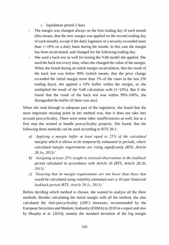
105

o liquidation period 2 days

- The margin was changed always on the first trading day of each month

(this means, that the new margin was applied on the second trading day

of each month), except if the daily logreturn of a security exceeded more

than +/-10% on a daily basis during the month. In this case the margin

has been recalculated, and changed for the following trading day.

- She used a back test as well for testing the VaR model she applied. She

used the back test every time, when she changed the value of the margin.

When she found during an initial margin recalculation, that the result of

the back test was below 99% (which means, that the price change

exceeded the initial margin more than 1% of the cases in the last 250

trading days), she applied a 10% buffer within the margin, so she

multiplied the result of the VaR calculation with (1+10%). But if she

found that the result of the back test was within 99%-100%, she

disregarded the buffer (if there was any).

When she read through to adequate part of the regulation, she found that the

most important missing point in her method was, that it does not take into

account procyclicality. There were some other insufficiencies as well, but as a

first step she wanted to handle procyclicality properly. She found, that the

following three methods can be used according to RTS 28.1:

a) ‘Applying a margin buffer at least equal to 25% of the calculated

margins which it allows to be temporarily exhausted in periods, where

calculated margin requirements are rising significantly (RTS, Article

28.1a, 2013)’

b) ‘Assigning at least 25% weight to stressed observations in the lookback

period calculated in accordance with Article 26 (RTS, Article 28.1b,

2013).’

c) ‘Ensuring that its margin requirements are not lower than those that

would be calculated using volatility estimated over a 10 year historical

lookback period (RTS, Article 28.1c, 2013).’

Before deciding which method to choose, she wanted to analyze all the three

methods. Besides calculating the initial margin with all the method, she also

calculated the Anti-procyclicality (APC) measures, recommended by the

European Securities and Markets Authority (ESMA) in 2018 in a report and also

by Murphy et al. (2014), namely the standard deviation of the log margin

106

change, and the peak-to-through ratio, which means the ratio of the highest and

lowest margin value in the least 250 trading days.

Questions

1. Download the EMIR and the RTS to be able to answer the questions,

and read the Article 41 in EMIR and Chapter VI in RTS, which

regulates initial margin calculation!

2. Define initial margin for a freely chosen Asian stock with the method

created by Annie Li!

3. Calculate the initial margin for the same security with all the three

methods!

a. Create assumption for all of the three methods, where it is needed

to be able to calculate the initial margin. If you need help, the

following sources can be useful: Béli and Váradi (2016),

Berlinger et al (2016, 2018), Ladoniczki and Váradi (2018),

Murphy et al. (2014, 2016).

b. Plot figures on the time series of the calculated initial margins!

4. What aspect should be taken into account when we would like to

decide which method to use? Point out the advantages and

disadvantages of each of the three methods!

5. Show how the three different initial margin method take into account

procyclicality based on the APC measures of ESMA (2018) and

Murphy et al. (2014)!

References

Béli, M. & Váradi, K. (2016). Alapletét meghatározásának lehetséges módszertana

[A possible methodology for determining initial margin] Financial and Economic

Review, Vol. 16. (2) pp. 119-147.

Berlinger, E., Dömötör B., Illés F. & Váradi K. (2016). A tőzsdei elszámolóházak

vesztesége (Loss of stock exchange clearing houses), Közgazdasági szemle, LXIII.

September

107

Berlinger, E., Dömötör B. & Illés, F. (2018). Optimal Margin Requirement.

Financial Research Letters. 2018 https://doi.org/10.1016/j.frl.2018.11.010

Berlinger, E., Dömötör, B., & Illés, F. (2019). Anti-cyclical versus Risk-sensitive

Margin Strategies in Central Clearing. Journal of International Financial Markets,

Institutions and Money. 62. pp. 117-131.

Csóka, P. & Herings P.J.J. (2018). Decentralized clearing in financial

networks. Management Science, 64 (10), pp. 4681-4699

Cont, R. (2015). The end of the waterfall: Default resources of central

counterparties. Journal of Risk Management in Financial Institutions, Vol. 8. (4)

pp. 365-389.

ESMA – European Securites and Markets Authority (2018). Final Report –

Guidelines on EMIR Anti-Procyclicality Margin Measures for Central

Counterparties. 28th May. 2018. Available at:

https://www.esma.europa.eu/sites/default/files/library/esma70-151-

1293_final_report_on_guidelines_on_ccp_apc_margin_measures.pdf

EMIR – European Market Infrastructure Regulation: Regulation (EU) No

648/2012 of the European Parliament and of the Council of 4th July 2012 on the

OTC derivatives, central counterparties and trade repositories (EMIR - European

Market Infrastructure Regulation) Available: http://eur-lex.europa.eu/legal-

content/EN/TXT/PDF/?uri=CELEX:32012R0648&from=EN downloaded: 8th

February 2019.

Glasserman, P. & Wu, Q. (2017). Persistence and Procyclicality in Margin

Requirements. Columbia Business School Research Paper No. 17-34

Jorion, P. (2007): Value at risk: the new benchmark for managing financial risk.

Vol. 3. New York: McGraw-Hill

Ladoniczki, S. K. & Váradi, K. (2018). Elszámolóházak alapbiztosítéki

követelményeinek számítási módszertana (Calculation of initial margin of central

counterparties). Közgazdasági Szemle, Vol. 65. No. 4. pp. 780-809.

Murhpy, D., Vasios, M. & Vause, N. (2014). An investigation into the

procyclicality of risk-based initial margin models. Bank of England, Financial

Stability Paper No. 28.

Murphy, D. (2017). I’ve got you under my skin: large central counterparty financial

resources and the incentives they create Journal of Financial Market

Infrastructures 5(3) pp. 57–74

Murphy, D., Vasios, M. & Vause, N., (2016). A comparative analysis of tools to

limit the procyclicality of initial margin requirements. Bank of England Working

Paper No. 597.

https://doi.org/10.1016/j.frl.2018.11.010

https://doi.org/10.1287/mnsc.2017.2847


https://www.esma.europa.eu/sites/default/files/library/esma70-151-1293_final_report_on_guidelines_on_ccp_apc_margin_measures.pdf

https://www.esma.europa.eu/sites/default/files/library/esma70-151-1293_final_report_on_guidelines_on_ccp_apc_margin_measures.pdf

http://eur-lex.europa.eu/legal-content/EN/TXT/PDF/?uri=CELEX:32012R0648&from=EN


108

Naffa H. & Kaliczka N. (2011). Az állami szerepvállalás egy modellje a lejárt

követelések piacán, Hitelintézeti Szemle, 10 : 2 pp. 93-107., 15 p.

Platt, C., Csóka, P. & Morini, M. (2017). Implementing Derivatives Clearing on

Distributed Ledger Technology Platforms. R3 Reports, available at:

https://www.r3.com/wp-content/uploads/2017/11/implementing-derivatives-

clearing_R3_.pdf

RTS – Technical Standard: Commission delegated regulation (EU) 153/2013 of

19th December 2012 supplementing Regulation (EU) No 648/2012 of the European

Parliament and of the Council with regard to regulatory technical standards on

requirements for central counterparties. Available: http://eur-

lex.europa.eu/LexUriServ/LexUriServ.do?uri=OJ:L:2013:052:0041:0074:EN:PD

F downloaded: 8th January 2019.

Szanyi, Cs., Szodorai, M. & Váradi, K. (2018). A supplement to the regulation of

anti-cyclical margin measures of clearing activities. SSRN working paper.

Available at: https://papers.ssrn.com/sol3/papers.cfm?abstract_id=3242078



https://www.r3.com/wp-content/uploads/2017/11/implementing-derivatives-clearing_R3_.pdf


http://eur-lex.europa.eu/LexUriServ/LexUriServ.do?uri=OJ:L:2013:052:0041:0074:EN:PDF



https://papers.ssrn.com/sol3/papers.cfm?abstract_id=3242078

109

15. MANAGING RISKS AND GETTING UNDER THE

CENTRAL COUNTERPARTY’S SKIN

Melinda Szodorai


This case study aims to show the composition of the default waterfall of a central

counterparty (from now on: CCP) in order to understand the importance of the

sensitivity of its structure.

A CCP’s leading role and purpose are to centralize counterparty risk

management in the financial markets that operate (Pirrong, 2011). The main idea

of CCPs is that trading through a CCP, a bilateral trade between two

counterparties is replaced by two symmetric trades between the CCP and each

counterparty (Berlinger et al. 2016, 2018). Cont et al. (2010), Iyer and Peydró

(2011) point out an essential function and benefit of these market infrastructures,

namely the prevention of adverse effects and spillover of a defaulting

counterparty. Compared to bilateral trading, where the default of one entity can

spread throughout the system leading to a chain of contagious defaults, by

multilateral netting among market participants there is higher transparency, risk-

sharing among members of the clearinghouse is achieved (Csóka and Herings,

2018). Also, there is no need of duplicative monitoring, and mitigation of

counterparty risk is managed through the CCP as members of the system are

insulated from each other's default, reducing frictions in commitments (Nosal,

2011, Platt et. al. 2017). Naffa and Kaliczka (2011) describe a new model to

operate under a regulated and transparent market to address the problem of

defaulted loans.

Central counterparties do mitigate counterparty risk and are prepared to

withstand under “extreme but plausible market conditions.” However, CCPs are

no panacea, as if distress hits the financial system, CCPs are not an exception of

harsh aftermath. While CCPs provide protection against idiosyncratic

counterparty risk and serve as safeguards for the system as a whole, they offer

no essential protection against aggregate risk and may even encourage risk-

shifting (Biais et al. 2012). To avoid procyclical effects, the regulator requires

CCPs to apply an anticyclical margining, consequences of which is analyzed by

Berlinger et. al (2018, 2019). Another risk arises in current circumstances,

110

namely the default of the CCP itself. The default of a CCP, however, becomes

a systemic risk, triggering the collapse, or at least weakening the resilience of

an industry or economy. Duffie (2015) claims that in the case of this event,

financial stability would have dramatic effects. These situations are not

impossible. Since 1973 there were three events of this type and some near fail

situations as well (Kiff, 2014). There are further concerns regarding the

systematic importance pointed out by Markose et al. (2012). Learning from the

global financial crisis the too-big-to-fail problem may cause headaches for

everyone; CCPs also have a similar issue, the too-interconnected-to-fail

(Berlinger et al., 2016). This is similar to the other phenomena tightly related to

the moral hazard problem, meaning in the case of distress if CCPs would fail,

the adverse effects would be so wide-ranging that they could become prime

candidates to expect bailouts.

Regulators require CCP to operate a so-called default waterfall. A general

default waterfall consists of three main components: margins, default fund

contributions, and the CCP’s own dedicated resources. Regulations require

using the available balances in a preordered sequence:

1. In case of a default, the first resource to be used are the margins to cover

losses of the defaulting members, but not the margins provided by

surviving members. The value of the margins shall be procyclical

(Ladoniczki and Váradi, 2018, and Szanyi et al. 2018)

2. The second available financial resource is the contribution of members

to the mutualized fund of resources, the so-called default fund. The

primary goal of the default fund is that as members contribute to it, there

is loss-mutualization among them.

3. The third layer, if the previous resources are not enough to cover losses,

is the amount of the CCP’s own resources contributed to will be

exhausted. This is called the skin-in-the-game. It shall be higher by 25%

of the CCP’s required capital9.

The three components can be divided in more tranches, so in case of a default

the exhaustion of the available resources can be: initial margin of defaulting

member default fund contribution of defaulting member dedicated own

9 In line with EU legislation (EMIR, 2012) A CCP’s required capital shall at all times be

sufficient to ensure an orderly winding-down or restructuring of the activities over an

appropriate time span and an adequate protection of the CCP against credit, counterparty,

market, operational, legal and business risks.

111

resources of CCP default fund contribution of non-defaulting member

other financial resources of the CCP.

The methodology proposed by regulators aims to enforce the resilience of the

financial system by increasing transparency and market infrastructures that are

prepared to withstand extreme market events.

Case10

Charles Thomson focused intently on not letting his voice tremble as he ended

the call with another clearing member leaving the CCP. He opens the windows

of his office in Athens, Greece. Immediately he is hit by the vibrating sound of

the cars. He took a deep breath and tried to think. He has spent his whole

professional life working as a CEO of the Greek CCP.

Last year a speculative position of a clearing member blew a hole in the buffers

that shook the entire energy market. A trader had some risky positions in the

previous years as well, but luckily, it never ended with a loss. Currently, he built

up some speculative positions that the spread between the Greek and Estonian

power would open. Due to the stormy weather, the spread went right to the

opposite, and it narrowed. Although the CCP managed to handle the situation

by closing the massive amount of positions, the event had put its mark on the

mood of the market. Moreover, additional capital needed to be injected.

Shareholders showed their concern about the CCP’s future.

About the CCP

The CCP is a state-owned market infrastructure. Charles Thomson was the CEO

since it was established. They are a successful CCP all over Europe, being an

active and permanent member on foreign markets. It’s market presence grew in

the last few years, resulting in a robust increase in financial terms and also

achieved a much-diversified client portfolio, providing services for clearing

members from all over Europe. This year’s strategy is to continue the expansion.

In order to achieve this, the focus is on the acquisition of new customers, the

launch of new products, and the clearing of new markets. Thus, these are all

opportunities to increase volumes and to reach better economies of scale.

Organic expansion, maintaining a good relationship with the existing markets

and customers, and secure operation is the main strengths. The capital increase

10 The case is pure fiction. Any resemblance with reality is just coincidence.

112

was not part of the strategy, but it gave confidence in the CCP for market

participants, and business growth was achieved easier.

Since the market distress created by the defaulted speculative positions, the CCP

had to make some changes, especially in the pricing of the clearing service.

Changes in clearing

The default fund was a little part of the default waterfall system, and it was

composed mostly of the members’ margin and the CCP’s skin-in-the-game.

Charles experienced that this model fraught with moral hazard because clearing

members, having small real financial risk associated with the CCP, had little

incentive to monitor the quality of the CCP’s risk management or observe the

conduct of other clearing members in the marketplace. In the latter event,

closing the positions fell mostly upon the CCP. The skin-in-the-game amount

was quite high, but the fee structure adequate compared to the current industry

norms. It did not discourage members from taking excessive risks. The

margining model did not fail; the CCP demonstrated its confidence in its

margining models in the previous timeframe, but current events proved that a

highly concentrated default position, where the clearing member cannot meet

the margin call, exposes the CCP to excess risk.

Change in the default waterfall system was inevitable. The default fund

contribution was increased significantly. Taking the volume of the positions into

account, the default contribution for every member was increased, and everyone

was obligated to contribute on a pro-rata basis. The margining methodology

remains unchanged, but regulators require that stress shall be included in the

calculation methodology; therefore, current events increased the payments for

participants.

Low prices were the primary reason clients chose this CCP. Because prices are

converging towards West European CCPs’ prices, clearing members decide to

change.

Current year’s financial numbers are showing massive drops in revenues.

Shareholders ask Charles to rethink the company’s strategy in order to stop the

decrease of the client portfolio, but the CCP shall maintain a resilient position

on the market.

113

Questions

1. The CCP is a state-owned company. How does this fact affect the

incentives of market participants? What could the management do in

order to handle this? Would another increase in the capital be beneficial?

2. Why do you think clearing members abandon the CCP if prices are not

higher than the international ones?

3. If you were an appointed consultant specialized in risk management,

what options or alternatives would you suggest for Charles to resolve the

CCP’s situation?

References

Béli, M. & Váradi, K. (2016). Alapletét meghatározásának lehetséges

módszertana [A possible methodology for determining initial margin] Financial

and Economic Review, Vol. 16. (2) pp. 119-147.

Berlinger, E., Dömötör B., Illés F. & Váradi K. (2016). A tőzsdei

elszámolóházak vesztesége (Loss of stock exchange clearing

houses),Közgazdasági szemle, LXIII. September

Berlinger, E., Dömötör B. & Illés, F. (2018). Optimal Margin Requirement.

Financial Research Letters. 2018 https://doi.org/10.1016/j.frl.2018.11.010

Berlinger, E., Dömötör, B., & Illés, F. (2019). Anti-cyclical versus Risk-

sensitive Margin Strategies in Central Clearing. Journal of International

Financial Markets, Institutions and Money. 62. pp. 117-131.

Biais, B., Heider, F., Hoerova, M., 2012. Clearing, Counterparty Risk, and

Aggregate Risk. IMF Economic Review 60, 193–222.

Cont, R., 2010. Network structure and systemic risk in banking systems.

Working paper. https://ssrn.com/abstract=1733528 or

http://dx.doi.org/10.2139/ssrn.1733528

Csóka, P. & Herings P.J.J. (2018). Decentralized clearing in financial

networks. Management Science, 64 (10), 4681-4699.

Duffie, D., n.d. Resolution of Failing Central Counterparties, in Kenneth E.

Scott, Thomas H. Jackson & John B. Taylor, Making Failure Feasible, How

https://doi.org/10.1016/j.frl.2018.11.010

https://ssrn.com/abstract=1733528%20or%20http:/dx.doi.org/10.2139/ssrn.1733528

https://ssrn.com/abstract=1733528%20or%20http:/dx.doi.org/10.2139/ssrn.1733528



114

Bankruptcy Reform Can End “Too Big to Fail. Stanford, CA: Hoover Institution

Press) Working paper.

EMIR – European Market Infrastructure Regulation: Regulation (EU) No

648/2012 of the European Parliament and of the Council of 4th July 2012 on the

OTC derivatives, central counterparties and trade repositories (EMIR -

European Market Infrastructure Regulation) Available: http://eur-

lex.europa.eu/legal-content/EN/TXT/PDF/?uri=CELEX:32012R0648

&from=EN downloaded: 8th February 2019.

Iyer, R. & Peydró (2011). Interbank Contagion at Work: Evidence from a

Natural Experiment. The Review of Financial Studies 24, 1337–1377.

https://doi.org/10.1093/rfs/hhp105

Kiff, J., Dodd, R., Kazarian, E., Lustgarten, I., Sampic, C. & Singh, M., (2010).

Making Over-the-Counter Derivatives Safer: The Role of Central

Counterparties.

Ladoniczki, S. K. & Váradi, K. (2018). Elszámolóházak alapbiztosítéki

követelményeinek számítási módszertana (Calculation of initial margin of

central counterparties). Közgazdasági Szemle, Vol. 65. No. 4. pp. 780-809.

Markose, S., Giansante, S. & Shaghaghi, A. (2012). Too interconnected to fail”,

Financial network of US CDS Market: topological fragility and systemic risk.

Journal of Economic Behavior and Organization 83, 627–646.

McPartland, J. & Lewis, R. (2017). The Goldilocks problem: How to get

incentives and default waterfalls “just right.” Economic Perspectives, Federal

Reserve Bank of Chicago, (1).


követelések piacán, Hitelintézeti Szemle, 10(2) pp. 93-107.

Nosal, E. n.d. Clearing Over-The-Counter Derivatives. Economic Perpectives

4, pp. 137–145.

Pirrong, C. n.d. A Bill of Goods: CCPs and Systemic Risk. Journal of Financial

Market Infrastructures 2, pp. 55–85.

Platt, C., Csóka, P. & Morini, M. (2017). Implementing Derivatives Clearing on

Distributed Ledger Technology Platforms. R3 Reports, available

at: https://www.r3.com/wp-content/uploads/2017/11/implementing-

derivatives-clearing_R3_.pdf

Szanyi, Cs., Szodorai, M. & Váradi, K. (2018). A supplement to the regulation

of anti-cyclical margin measures of clearing activities. SSRN working paper.

Available at: https://papers.ssrn.com/sol3/papers.cfm?abstract_id=3242078




https://doi.org/10.1093/rfs/hhp105





https://papers.ssrn.com/sol3/papers.cfm?abstract_id=3242078

115

16. CREDIT RISK MEASURING

Barbara Dömötör


Credit risk is the most important risk type financial institutions are facing, and

it is responsible for the majority of their capital need. The aim of this study is to

present the main terms and calculations that the recent regulation applies in

connection with credit risk.

Credit risk is defined as the risk of potential losses deriving from non-payment

(default) or the change in the credit rating of a borrower, bond issuer or

counterparty in a derivative transaction (Hull, 2015). The creditworthiness is

described by the credit rating that reflects the non-performance probability of a

borrower. Naffa and Kaliczka (2011) describe a new model for public role in

tackling the issue of defaulted loans. Csóka and Herings (2019) model the

possible losses using cooperative game theory. About measuring credit risk and

the ratings at commercial banks see Walter (2014) about detailed analysis of

parameters and evaluation of credit risk in the case of project financing see

Walter (2019).

The expected loss on a credit depends on three factors:

- the probability of default (PD): the probability that the borrower goes

bankrupt during the lifetime of the loan or bond. PD refers always to a

given period, most frequently for the next one year. Being a probability,

PD can take any values between zero and one.

- the loss given default (LGD): the proportion of the exposure that will be

lost (not recovered) in case of default. Expressed in percentage.

Recovery rate (RR) is the complementary of LGD: 𝐿𝐺𝐷 = 1 − 𝑅𝑅

- the exposure at default (EAD): the exposure expressed in absolute value

(USD, EUR, etc)

To model the loss distribution all above parameters should be estimated.

Exposure is easy to calculate for standard loans, but its value depends on market

variables as well, in the case of derivatives contracts. Loss can be mitigated if

the debt is secured by collateral, or guarantee, or netting arrangements apply.

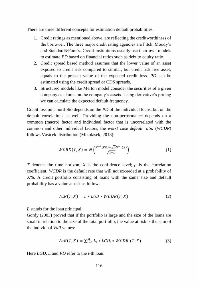
116

There are three different concepts for estimation default probabilities:

1. Credit ratings as mentioned above, are reflecting the creditworthiness of

the borrower. The three major credit rating agencies are Fitch, Moody’s

and Standard&Poor’s. Credit institutions usually use their own models

to estimate PD based on financial ratios such as debt to equity ratio.

2. Credit spread based method assumes that the lower value of an asset

exposed to credit risk compared to similar, but credit risk free asset,

equals to the present value of the expected credit loss. PD can be

estimated using the credit spread or CDS spreads.

3. Structured models like Merton model consider the securities of a given

company as claims on the company’s assets. Using derivative’s pricing

we can calculate the expected default frequency.

Credit loss on a portfolio depends on the PD of the individual loans, but on the

default correlations as well. Providing the non-performance depends on a

common (macro) factor and individual factor that is uncorrelated with the

common and other individual factors, the worst case default ratio (WCDR)

follows Vasicek distribution (Mikolasek, 2018):

𝑊𝐶𝑅𝐷(𝑇, 𝑋) = 𝑁 (𝑁−1(𝑃𝐷)+√𝜌𝑁−1(𝑋)

√1−𝜌) (1)

T denotes the time horizon; X is the confidence level; 𝜌 is the correlation

coefficient. WCDR is the default rate that will not exceeded at a probability of

X%. A credit portfolio consisting of loans with the same size and default

probability has a value at risk as follow:

𝑉𝑎𝑅(𝑇, 𝑋) = 𝐿 ∗ 𝐿𝐺𝐷 ∗ 𝑊𝐶𝐷𝑅(𝑇, 𝑋) (2)

L stands for the loan principal.

Gordy (2003) proved that if the portfolio is large and the size of the loans are

small in relation to the size of the total portfolio, the value at risk is the sum of

the individual VaR values:

𝑉𝑎𝑅(𝑇, 𝑋) = ∑ 𝐿𝑖 ∗ 𝐿𝐺𝐷𝑖 ∗ 𝑊𝐶𝐷𝑅𝑖(𝑇, 𝑋)𝑀𝑖=1 (3)

Here LGD, L and PD refer to the i-th loan.

117

The regulation requires that the equity should be appropriate to absorb a

potential loss with a high probability, so the capital need corresponds to a high

confidence level (99.9%) value at risk with a one-year time horizon. In the case

of credit risk, financial institutions are prepared for the expected value of credit

loss by their pricing or profit reduction, so capital requirement refers to the

difference of the VaR and the expected loss, the so called unexpected loss.

Regulation

Capital requirement for credit risk is also regulated in EU No 575/2013

Regulation (CRR). CRR offers, similarly to market risk, two approaches to

determine own funds need for credit risk: the standardized approach and Internal

Ratings Based (IRB) approach. The capital requirement equals to 8 percent (this

is the famous Cook ratio) of the risk weighted exposure. The two above

approaches differ in the determination of the risk weighted exposure. In the case

of the standardized approach all exposures shall be assigned to one of the given

(16) exposure classes, and the risk weights depend on the exposure class and the

credit quality of the exposure. Risk weights range from 0 to 150%. Risk weights

(RW) are allowed to be adjusted for collaterals.

Internal ratings based method can be used upon approval of the appropriate

authorities. The risk weighted exposure is determined by the given weighting

function that has the following form.

For corporate, sovereign and bank exposures:

𝑅𝑊 = 𝐿𝐺𝐷 ∗ (𝑊𝐶𝑅𝐷 − 𝑃𝐷) ∗ 𝑀𝐴 ∗ 12.5 ∗ 1,06 (4)

118

WCRD shall be calculated as shown above. The calculation of the correlation

coefficient (𝜌) and the maturity adjustment (MA) are to be calculated as follows.

𝜌 = 0.12 ∗ 𝑥 + 0.24 ∗ (1 − 𝑥) (5)

𝑥 =1−𝑒−50∗𝑃𝐷

1−𝑒−50 (6)

𝑀𝐴 =1+(𝑀−2.5)∗𝑏

1−1.5∗𝑏 (7)

𝑏 = [0.11852 − 0.05478 ∗ ln (𝑃𝐷)]2 (8)

Parameter M denotes the maturity of the exposure.

We can see that the correlation coefficient is between 0.12 and 0.24, and

decreases, goes to its lower bound, if PD increases. The argument behind is that

if the default probability increases, default becomes more idiosyncratic and less

dependent by the common, market factor.

As PD refers to one-year, maturity adjustment serves for quantifying the loss on

a longer asset, deriving from the change in riskiness (PD).

The risk weighted asset (RWA) that is to be multiplied by the Cook ratio to get

capital requirement is:

𝑅𝑊𝐴 = 𝑅𝑊 ∗ 𝐸𝐴𝐷 (9)

IRB approach includes two methods:

- Foundation IRB Approach: in this case PD is calculated by the financial

institution, but LGD, EAD, M are determined by the regulation.

- Advanced IRB allows financial institutions to use own calculations for

all parameters.

Risk weight for retail exposure is to be calculated similarly, with the difference

that there is no maturity adjustment and the correlation coefficient is set between

0.03 and 0.16.

𝑅𝑊 = 𝐿𝐺𝐷 ∗ (𝑊𝐶𝑅𝐷 − 𝑃𝐷) ∗ 12.5 ∗ 1,06 (10)

𝜌 = 0.03 ∗ 𝑥 + 0.16 ∗ (1 − 𝑥) (11)

𝑥 =1−𝑒−35∗𝑃𝐷

1−𝑒−35 (12)

119

For residential mortgages 𝜌 is set the 0.15 and for qualifying revolving

exposures to 0.04.

For retail exposures all banks are using their own estimates for PD, LGD and

EAD (Hull, 2015).

Case

The Bank has the following credit portfolio:

a) 5-year loan of 100 million USD to European Bank for Reconstruction

and Development;

b) 500 million HUF unsecured loan to MOL Nyrt. with a maturity of 10

years;

c) 250 million HUF loan to Richter Nyrt. secured by immovable mortgage

of 150 million HUF;

d) 200 million HUF loan to a medium sized, BBB rated company with a

state guarantee for 90% of the exposure;

e) 3-years loan of 70 million HUF to a small enterprise secured by

mortgage of 30 million HUF;

f) Personal loan commitment of 2 million HUF;

The credit ratings and Bloomberg’s default risk calculations for the two

exchange traded companies (MOL and Richter) can be found below.

120

Source: Bloomberg

Source: Bloomberg

121

Questions / exercises

1. Explain the main differences of the Standardized and Internal Ratings

Based methods in calculation of capital requirements!

2. Draw a chart showing the worst case default ratio at 99.9% confidence

level in the function of PD and 𝜌, based on a one factor Gaussian copula

model!

3. Calculate the own funds requirement of the Banks’s credit portfolio

according to the standardized approach of EU No. 575/2013 Regulation

(Capital requirement for credit risk, Chapter 2)! Describe the

assumptions and concepts underlying the determination of risk

weighted assets and risk mitigation techniques and the Credit

Conversion Factors, if applicable.

4. Calculate the own funds requirement of the credit portfolio according

to the foundation IRB approach! Use your own estimates, if necessary!

5. Suppose that a 3-year zero-coupon Treasury bond with a face value of

100 yields 5% and a similar 3-year zero-coupon bond issued by a

corporation yields 5.5%. (Both rates are effective rates.) Make the

simplifying assumption that there are no recoveries in the event of a

default. Determine the probability of default! Determine the probability

of default in the function of various recovery rates!

References

Csóka, P.& Herings, P.J.J. (2019). Liability games. Games and Economic

Behavior, 116, 260-268.

EU No. 575/2013 Regulation: Capital requirement regulation available:

https://eur-lex.europa.eu/legal-

content/EN/TXT/PDF/?uri=CELEX:32013R0575&from=EN

Hull, J. (2012). Risk management and financial institutions,+ Web Site (Vol.

733). John Wiley & Sons.

Mikolasek, A. (2018). Problems in the Application of Credit Risk Models.

Economy and Finance, 3(5), 240-249.

https://doi.org/10.1016/j.geb.2019.05.007

122


követelések piacán, Hitelintézeti Szemle, 10(2) pp. 93-107.

Walter, Gy. (2014). Kereskedelmi banki ismeretek, Alinea, Budapest

Walter, Gy. (2019). Risk-adjusted pricing of project loans. Studies in Economics

and Finance, Vol. ahead-of-print No. ahead-of-print.

https://doi.org/10.1108/SEF-05-2018-0149



https://doi.org/10.1108/SEF-05-2018-0149

Documents

SELECTED CHAPTERS OF CORPORATE FINANCE AND RISK …