Seismic Hazard Curves and Uniform Hazard Response Spectra for the United States by A. D. Frankel and E. V. Leyendecker

A User Guide to Accompany Open-File Report 01-436

2001

This report is preliminary and has not been reviewed for conformity with U.S. Geological Survey editorial standards or with the North American Stratigraphic Code. Any use of trade firm or product names is for descriptive purposes only and does not imply endorsement by the U.S. Government.

U.S. DEPARTMENT OF THE INTERIORGale A. Norton, SecretaryU.S. GEOLOGICAL SURVEYCharles G. Groat, Director

Seismic Hazard Curves and Uniform Hazard Response Spectra for the United States

A User Guide to Accompany Open-File Report 01-436

A. D. Frankel1 and E. V. Leyendecker2

ABSTRACT

The U.S. Geological Survey (USGS) recently completed new probabilistic seismic hazard maps for the United States. The hazard maps form the basis of the probabilistic component of the design maps used in the 2000 International Building Code (International Code Council, 2000a), 2000 International Residential Code (International Code Council, 2000a), 1997 NEHRP Recommended Provisions for Seismic Regulations for New Buildings (Building Seismic Safety Council, 1997), and 1997 NEHRP Guidelines for the Seismic Rehabilitation of Buildings (Applied Technology Council, 1997). The probabilistic maps depict peak horizontal ground acceleration and spectral response at 0.2, 0.3, and 1.0 sec periods, with 10%, 5%, and 2% probabilities of exceedance in 50 years, corresponding to return times of about 500, 1000, and 2500 years, respectively.

This report is a user guide for a CD-ROM that has been prepared to allow the determination of probabilistic map values by latitude-longitude or zip code. The CD includes additional spectral accelerations at 0.1, 0.5, and 2.0 sec for the 48 conterminous states. The CD also contains hazard curve data that were used to prepare the maps. Hazard curves may also be determined by latitude-longitude or zip code.

_______________________________ 1 Geophysicist, U.S. Geological Survey, MS 966, Box 25046, DFC, Denver, CO, 80225 2 Research Civil Engineer, U.S. Geological Survey, MS 966, Box 25046, DFC, Denver, CO, 80225

1

INTRODUCTION

In June 1996 the USGS completed new national seismic hazard maps for the conterminous United States. These maps were placed on the Internet (http://geohazards.cr.usgs.gov/eq/) and subsequently published as large format maps. There are two sets of maps available for the 48 conterminous states. The first set covers all 48 states (Frankel et al., 1997 a), the second set is for region A of Figure A (Frankel et al., 1997 b). This regional set of maps covers California, Nevada, and portions of western Utah and Arizona. Each set of these hazard maps includes maps of peak horizontal ground acceleration and spectral response at 0.2, 0.3, and 1.0 sec periods, for 10%, 5%, and 2% probabilities of exceedance in 50 years. These probabilities of exceedance correspond to return times of about 500, 1000, and 2500 years, respectively. New hazard maps for Alaska (Wesson et al., Figure A. Regional map A. The regional map includes1999 a, b) and Hawaii (Klein et al., 2000) California, Nevada, and western portions of Utah andhave recently been completed. Each set of Arizona.these hazard maps includes maps of peakhorizontal ground acceleration and spectral response at 0.2, 0.3, and 1.0 sec periods, for 10% and 2% probabilities of exceedance in 50 years, corresponding to return times of about 500 and 2500 years, respectively. The 5% probability of exceedance maps were omitted for Alaska andHawaii after it was found that the demand for these maps was limited. The methodology used for preparation of the maps is documented in Frankel et al (1996), Wesson et al (1999), and Klein et al (draft, 1998). Copies of these reports are included with this CD-ROM. A summary paper describing the hazard maps is available in a special edition of Spectra (Frankel et al., 2000).

The mapping project was part of “Project 97" with the Building Seismic Safety Council (BSSC) to produce seismic design maps for the 1997 NEHRP Recommended Provisions for Seismic Regulations for New Buildings (hereafter referred to as NEHRP Provisions). The design maps in the 1997 NEHRP Provisions are a combination of probabilistic seismic hazard maps for most of the U.S. and deterministic hazard maps near specific faults in California, Oregon, Washington, Alaska, and Hawaii. The design maps originally prepared for the NEHRP Provisions have also been adopted for use in the 1997 NEHRP Guidelines for the Seismic Rehabilitation of Buildings (ATC, 1997), International Building Code (ICC, 2000), and the International Residential Code (ICC, 2000). A summary paper describing the design maps is also available in the special edition of Spectra (Leyendecker et al., 2000) mentioned above.

2

The hazard maps serve a number of purposes, e.g. site studies, structural design, earthquake loss studies, etc. Although simple in approach, it can be cumbersome to work with multiple maps. In order to simplify use of the ground motion maps the CD-ROM described in this report was prepared. The original intent of the CD-ROM was to enable a user to determine map values for a site by zip code or latitude-longitude. However, it was soon discovered that the possibilities were much broader.

The CD-ROM provides three basic sets of information to the user (1) map files, (2)hazard curve data, and (3) spectral response acceleration data. The hazard curve and spectral response acceleration data may be obtained in tabular or graphical form by specifying a site location by latitude-longitude or zip code. The CD also contains the map files for the four map sets described earlier.

The data base used with the CD-ROM is the same as that used to prepare the maps. The parameters used to prepare each map were calculated on a grid for the areas to be mapped, the maps were then constructed by contouring the “gridded data”. The grid spacing was 0.1 deg for the 48 conterminous states (except Region A was also calculated at a grid of 0.05 deg) and Alaska. Hawaii maps were constructed using calculations at a grid spacing of 0.02 deg.

SOFTWARE AND USER GUIDE

A program, Probabilistic Hazard 3.10, was written to retrieve the various data on the CD. The program was written in Visual Basic 6.0 to operate on a PC with a Windows 95 or later operating system. It self installs and uses the usual mouse and point and click approach to operate. The program allows the user to calculate both a hazard curve and a uniform hazard response spectrum for a specified site. The program also opens the map files for viewing. Some of the program features are described below. More detail is provided in Figures 1 through 16 with the detailed information in the figure captions. Table 1 shows the general information for installing and operating the software.

HAZARD MAPS

All of the maps in the four map sets of the United States described in the Introduction are included in the subdirectory “GM96-MAPS” on the CD-ROM, in pdf format. The program, Probabilistic Hazard 3.10, is used to view the various maps by selecting from a list of the maps. Once a map is selected, the program opens Acrobat Reader (copyright Adobe) with the map. The program uses Acrobat Reader to view and manipulate the maps, such as zooming and printing. The maps may also be viewed using Acrobat Reader independently of Probabilistic Hazard.

3

HAZARD CURVES A sample hazard curve is shown in Figure B. A hazard curve, as calculated on the CD, is a

plot of the annual frequency of exceedance (FEX) versus peak ground acceleration or one of the spectral accelerations. The hazard curve for peak ground acceleration shown in Figure B was calculated for a specific site, located by latitude-longitude, by interpolating data at the surrounding four grid points. Data used to prepare the graph are also tabulated along with the plot. The program allows the user to print the data in hard copy or save it in an ASCII comma-delimited file. Data saved in this type of file can be imported into a large variety of software, such as a spreadsheet program, for additional processing as specified by the user.

The maps were prepared by computing such hazard curves at each grid point within the mapping area. FEX values of 0.0021, 0.00103, and 0.000404 correspond to Figure B. Sample seismic hazard probabilities of exceedance of 10% in 50 years, 5% in 50 curve for peak ground years, and 2% in 50 years respectively. The hazard curve acceleration Data points are was then used to determine the acceleration value shown as solid circles. corresponding to each of these three FEX values and stored in a data base. This procedure was repeated at each grid point, for each ground motion parameter. This process created the “gridded data” referred to above that was used to prepare the maps.

RESPONSE SPECTRA Although maps were not made, hazard curves were also developed for spectral accelerations

at 0.1, 0.5, and 2.0 sec for the 48 conterminous states in addition to hazard curves for peak ground acceleration and spectral accelerations at 0.2, 0.3, and 1.0 sec. These additional values were not computed for Hawaii or Alaska because appropriate ground motion attenuation equations were not available for these periods for these geographical regions. The peak ground acceleration and spectral accelerations corresponding to each of the three standard probabilities were used to create a data base for response spectra for the three probability levels at each grid point. A sample response spectrum for a 2% probability of exceedance in 50 years is shown in Figure C. Response spectra can also be computed for 5% Figure C. Sample uniform hazard and 10% probability of exceedance in 50 years. As was the response spectrum for 2% PE in case for hazard curves, data used to prepare the graph are 50 years. also tabulated. The program allows the user to print the data in hard copy or save it in an ASCII comma-delimited file. The current version of the software does not allow saving the graph in a separate file.

4

CONCLUDING REMARKS

The CD-ROM has been developed to simplify obtaining mapped ground motions and hazard. The CD is intended to be as user friendly as possible and to quickly give the user the data needed for various purposes, such as design or site studies. The intent of USGS is to simplify and reduce the time required to obtain data from a large set of maps.

It should be noted that the values obtained from the CD are the same as the values for the probabilistic component of the design maps in NEHRP Provisions and the other design documents which have incorporated the design maps. However, the probabilistic values differ from the deterministic component of the design maps.

As previously indicated, the user guide is developed as a series of figures numbered Figure 1 through 16 following this text. Each figure is a screen copy obtained while running the program. The caption for each figure contains extensive text so the user does not have to go back and forth between text and figure. The figures go through an example for calculating a response spectrum in some detail, followed by an example for calculating a hazard curve. Use of the map viewer capability is also illustrated. It is suggested the user run the software using the information in the figures as a tutorial to gain experience in using the software.

Comments and suggestions are welcome and may be sent to the individuals named below:

E. V. Leyendecker A. D. Frankelemail - leyendecker@usgs.gov email - afrankel@usgs.govPhone 303-273-8565 Phone 303-273-8556FAX 303-273-8600 FAX 303-273-8600U. S. Geological Survey U. S. Geological SurveyP. O. Box 25046, MS 966 P. O. Box 25046, MS 966Denver, CO 80225 Denver, CO 80225

ACKNOWLEDGMENTS

The authors received comments and suggestions from many individuals while preparing this version of the CDROM. These suggestions are gratefully acknowledged. Two individuals, Richard D. McConnell and Michael Valley, were particularly thorough and offered many well-considered suggestions, most of which were incorporated into this version of the software on the CD-ROM.

5

REFERENCES

Applied Technology Council, 1997, NEHRP Guidelines for the Seismic Rehabilitation of Buildings, FEMA 273, Washington, D. C.

Building Seismic Safety Council, 1998, NEHRP Recommended Provisions for Seismic Regulations for New Buildings and Other Structures, FEMA 302, Part 1- Provisions, FEMA 303, Part 2 -Commentary, Washington, D.C.

Frankel A.D., Mueller, C.S., Barnhard, T.P., Perkins, D.M., Leyendecker, E.V., Dickman, N.C., Hanson, S.L., and Hopper, M.G., 1996, National Seismic Hazard Maps, June 1996: Documentation, U.S. Geological Survey, Open-file Report 96-532.

Frankel A.D., Mueller, C.S., Barnhard, T.P., Perkins, D.M., Leyendecker, E.V., Dickman, N.C., Hanson, S.L., and Hopper, M.G., 1997a, Seismic - Hazard Maps for the Conterminous United States: U.S. Geological Survey, Open-file Report 97-130, 12 sheets, scale 1:7,000,000.

Frankel A.D., Mueller, C.S., Barnhard, T.P., Perkins, D.M., Leyendecker, E.V., Dickman, N.C., Hanson, S.L., and Hopper, M.G., 1997b, Seismic-Hazard Maps for the California, Nevada and Western Arizona/Utah: U.S. Geological Survey, Open-file Report 97-130, 12 sheets, scale 1:2,000,000.

Frankel, A.D., Mueller, C.S., Barnhard, T.P., Leyendecker, E.V., Wesson, R.L., Harmsen, S.C., Klein, F.W., Perkins, D.M., Dickman, N.C., Hanson, S.L., and Hopper, M.G., 2000, AUSGS National Seismic Hazard Maps”, Spectra, Earthquake Engineering Research Institute, Oakland, CA.

International Code Council, Inc., 2000a, International Building Code, Building Officials and Code Administrators International, Inc., Country Club Hills, IL; International Conference of Building Officials, Whittier, CA; and Southern Building Code Congress International, Inc., Birmingham, AL.

International Code Council, Inc., 2000b, International Residential Code, Building Officials and Code Administrators International, Inc., Country Club Hills, IL; International Conference of Building Officials, Whittier, C. A., and Southern Building Code Congress International, Inc., Birmingham, AL.

Klein, F.W., Frankel, A.D., Mueller, C.S., Wesson, R.L., and Okubo, P.G., 1998 (draft), Documentation for Seismic Hazard Maps for the State of Hawaii (draft), available in draft form.

Klein, F.W., Frankel, A.D., Mueller, C.S., Wesson, R.L., and Okubo, P.G., 2000, Seismic - Hazard Maps for Hawaii: U.S. Geological Survey, Geologic Investigation Series Maps I-2724, 2 sheets.

Leyendecker, E. V., Hunt, R. J., Frankel, A. D., and Rukstales, K. S., 2000. “Development of Maximum Considered Earthquake Ground Motion Maps”, Spectra, Earthquake Engineering Research Institute, Spectra , Oakland, CA.

Wesson, R.L., Frankel A.D., Mueller, C.S., and Harmsen, S.C., 1999, Probabilistic Seismic Hazard Maps of Alaska, U.S. Geological Survey, Open-file Report 99-36.

Wesson, R.L., Frankel A.D., Mueller, C.S., and Harmsen, S.C., 1999, Seismic - Hazard Maps for Alaska: U.S. Geological Survey, Geologic Investigation Maps I-2679, 2 sheets.

6

Table 1. General Instructions for the Program

Installation

Click on Start.Run Setup.exe in the root directory on the CDROM and follow

the instructions. You may be requested to update selected files. This is required. The program will be installed in the directory Probabilistic

Hazard 3.10 with an executable file named Probabilistic Hazard 3.10.exe.

System Requirements

A PC (or compatible) with Windows 95, Windows 98, or Windows NT.

Pentium Processor with 32 MB of RAM, 200 MHZ recommended.

A minimum screen resolution of at least 800 x 600. A hard drive with 30 MB available for installing the software.

Operation

Click on Start.Click on Programs.Select Probabilistic Hazard 3.10 from the Programs list or place

an icon on the Desktop.

Files

Random Access Data files are in the directory GM96-Data on the CD.

PDF Map files are in the directory GM96-Maps on the CD. Adobe Acrobat is required to view the maps. Acrobat Reader

version 4 is included on the CD. Version 4 is recommended for maximum benefit in viewing and printing the PDF map files.

7

Figure 1. Seismic Hazard Curves and Uniform Hazard Response Spectra. The opening screen contains controls for obtaining seismic data for both probabilistic hazard curves and response spectra. Typically a control may be accessed in three ways - (1) using the Mouse to place the cursor over the control and pressing the left Mouse button, (2) using the Tab key to cycle through the controls and pressing the Enter key, or (3) holding down the Alt key and pressing the underlined character on the key. Many users will find methods (1) and (3) a convenient way to move rapidly between controls and screens. Use whatever method or combination of methods is most convenient. Selecting the control labeled Hazard Curves and Response Spectra for the United States will open the screen shown in Figure 2. Figure 2 will be used to illustrate most of the controls and screens. The Exit Program control closes the program.

8

Figure 2. Uniform Hazard Spectra and Seismic Hazard Curves. Selecting the control discussed in Figure 1 opened the screen shown in this figure. The contents of the screen are accessed sequentially. Portions that can not be accessed are grayed out. In general, the user is guided through the program by the use of titles in red and controls with titles in black. This is a clue as to what control or option should be used next. At the point shown in the figure, the user may use the option for entering a name and date or proceed directly to the Open File Selection Menu control. Although not required, this option is a convenient way to include a name or project description in the output. The option is followed by selecting the Open File Selection Menu control. Throughout the program, “tool tips” (notes with a yellow background that explain the meaning or use of a control) will appear if the cursor is held over a control or option. Note that in this screen the user may return to the screen in Figure 1 by selecting the Opening Menu control. The Exit Program control closes the program.

9

Figure 3. Optional Name and Date Entry. The name and date option have been selected. Both will be included with the output calculations. If only one is selected, then only the one will be included. The date and time are the computer time. In this case a project description has been entered instead of a name. The name indicates that the following series of screens will be an example of determining a response spectrum.

In order to proceed, the user must select the Open File Selection Menu control.

10

Figure 4. Select File Locations. The data files and the map files may be accessed on the CD ROM or from a location on a hard drive or any other drive with sufficient space to hold them. In the case shown the directories containing the files have been copied to the C: drive. Location on a hard drive will usually allow faster access time than using the files located on the CD ROM. If the files are relocated, the names of the directories containing the files should be the same as those on the CD ROM, although this is not necessary. The user may also manually enter the location of files in the text boxes. An error message will appear if an incorrect drive is selected. The software checks to be sure that each data file and map file is in the designated directory. All files must be present before proceeding.

Once the location of the files has been entered, that location is remembered for future runs of the software. However, if the files are moved, a new path must be entered. Press OK to return to the main menu. As long as the correct file locations are shown in the text boxes, all the user has to do is click on OK, regardless of what is shown elsewhere on the screen.

11

Figure 5. Select Geographic Region. Geographic Regions may be selected by clicking on the text. The selected region is highlighted in blue. Site locations for the conterminous 48 states, Alaska, and Hawaii may be specified by latitude-longitude or zip code as shown in the Select Site Location frame. The so-called “radio buttons” may be used to select either method of locating a site. The buttons are shown in white and their descriptions are shown in blue. The control View Maps allows the user to access the maps used in the various design procedures. Notice that a list of parameters that now appears in the list box in the frame to Calculate UHS or Hazard Curve. These parameters may not be selected until the method of specifying a site has been specified.

12

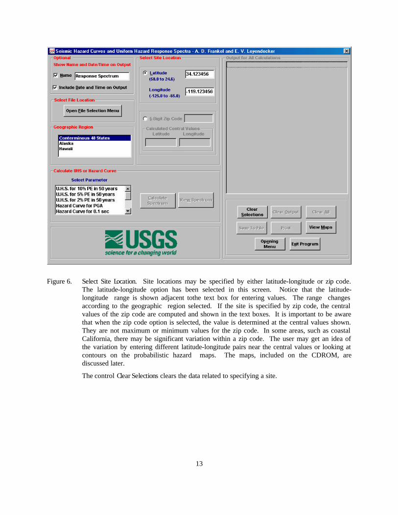
Figure 6. Select Site Location. Site locations may be specified by either latitude-longitude or zip code. The latitude-longitude option has been selected in this screen. Notice that the latitude-longitude range is shown adjacent tothe text box for entering values. The range changes according to the geographic region selected. If the site is specified by zip code, the central values of the zip code are computed and shown in the text boxes. It is important to be aware that when the zip code option is selected, the value is determined at the central values shown. They are not maximum or minimum values for the zip code. In some areas, such as coastal California, there may be significant variation within a zip code. The user may get an idea of the variation by entering different latitude-longitude pairs near the central values or looking at contours on the probabilistic hazard maps. The maps, included on the CDROM, are discussed later.

The control Clear Selections clears the data related to specifying a site.

13

Figure 7. Calculate Spectrum. The spectral values for the U.H.S. for 2% PE in 50 years (highlighted in blue) were calculated by pressing the Calculate Spectrum control. Notice the optional name and date are shown with the output. The latitude and longitude used to calculate the values are also shown so there is a record of the input along with the output. The values are calculated by interpolation using the four surrounding grid points. These grid points are in the data files in the directory GM96-Data on the CD. Data are located at different grid spacing for different regions. In the case shown the grid spacing is 0.05 degree. In the central and eastern United States the spacing is 0.1 degree. This latter spacing would not be adequate for a region such as the southwestern United States, particularly California, where there are many faults. The Alaska grid spacing is 0.1 degree and the Hawaii grid spacing is 0.02 degree.

There are four additional controls shown below the output box that are now active. These are described below:

Clear Output clears the contents of the output box.

Clear All combines Clear Selections and Clear Output.

Save To File saves the contents of the output box to an ASCII comma-delimited file.

Print sends the contents of the output box to a printer.

14

Figure 8. Response Spectrum Plot. A spectrum based on the data in Figure 7 is shown in the plot. The spectral values are shown as solid blue circles. The values used to prepare the plot are shown in the adjacent list box. These are the same as those in the output box shown in Figure 7. The plot includes data, site location, soil factors, and type of ground motion (2% in 50 years in this case). The plot and its data points may be printed by selecting Print Spectrum. In the current version of the software, the figure may not be saved as a file.

15

Figure 9. Calculate Spectrum for Alaska. In this example, the spectral values were calculated for a location in Alaska for a U.H.S. for 10% PE in 50 years (highlighted in blue). It may be observed that the calculations are cumulative with the calculations in Figure 7. Calculations will not be cumulative if the Clear Output control is pressed between calculations. It may also be observed that there are not as many spectral values for the site in Alaska as there were in the lower 48 states. Locations in Alaska and Hawaii do not have spectral values calculated for periods of 0.1, 0.5, and 2.0 sec because there were not appropriate attenuation functions for these periods in these two geographical regions.

16

Figure 10. Response Spectrum Plot for Alaska. The data in Figure 9 are shown in the plot. The spectral values are shown as solid red circles. The main difference between the content of this plot and the one shown in Figure 8 (other than the different location) is that dashed lines are drawn through the data. The lines are shown dashed to illustrate the general trends of the data although, due to the lack of additional spectral values, it is considered more appropriate to leave interpretation of the intermediate values to the judgment of the professional using the data. These same remarks apply to spectral plots for sites in Hawaii.

17

Figure 11. Calculate Hazard Curve. The hazard curve for peak ground acceleration (highlighted in blue) was calculated by pressing the Calculate Hazard Curve control. Notice that the names of the “Calculate” and “View” controls have changed from the names in Figure 9. These controls depend on whether the selected parameter is a U.H.S. or a Hazard Curve. In this example, a zip code was used to specify the site. The latitude and longitude are the central values for the zip code. These values are in the program data base for the zip code. As previously noted, it is important to be aware that when the zip code option is selected, the ground motion parameters are determined at the central values shown. They are not maximum or minimum values for the zip code. In some areas, such as coastal California, there may be significant variation within a zip code. The zip code and the latitude-longitude used to calculate the values are also shown in the output so there is a record of the input along with the output. The hazard curve values are interpolated to the site based on the surrounding four grid points. This is the same procedure used to interpolate the spectral values.

18

Figure 12. Hazard Curve Plot. A hazard curve based on the data in Figure 11 is shown in the plot. The data are shown as solid blue circles. The values used to prepare the plot are shown in the adjacent list box. These are the same as those in the output box shown in Figure 11. The plot includes data, site location, site condition, and type of hazard curve (PGA in this case). The plot and its data points may be printed by selecting Print Hazard Curve. The figure may not be saved as a separate file.

FEX is the annual frequency of exceedance. The user is cautioned that values smaller than 10-4 should be used with carefully. This precaution is because such values are usually associated with critical structures. Such structures frequently warrant special site study considerations that may or may not have been incorporated in the national maps. FEX values of 0.0021, 0.00103, and 0.000404 correspond to probabilities of exceedance of 10% in 50 years, 5% in 50 years, and 2% in 50 years respectively.

19

Figure 13. Select Map File. The maps may be viewed at any time after the file locations have been specified. Clicking on the View Maps control shown Figure 5, 6, or 7 opens the menu shown. Click on a map to enable the View Map button. Click the View Map control to load the map. The map sets include the probabalistic maps for the 48 conterminous states, the southwestern U.S., Alaska, and Hawaii. The map selected above is shown in Figure 14.

Selecting the control Notes for First Time Users opens the screen in Figure 15. Selecting the control Select New Path for Acrobat Reader opens the screen shown in Figure 16.

20

The

map

sho

wn

isT

he p

rogr

am a

utom

atic

ally

ope

ns A

crob

at R

eade

r an

d lo

ads

the

map

file

.A

crob

at R

eade

r. di

ffic

ult t

o re

ad b

ecau

se it

is a

red

uctio

n fr

om th

e or

igin

al s

ize

of a

bout

24"

x 3

6".

It b

ecom

es e

asie

r to

rea

d w

hen

the

Aft

er z

oom

ing

in,

the

grap

hics

sel

ect

tool

can

be

used

to

sele

ctm

agni

fica

tion

tool

is

used

to

zoom

int

o an

are

a.

deta

iled

port

ions

of

the

map

for

pri

ntin

g. U

se th

e Cl

ose

Map

con

trol

to c

lose

the

read

er.

Figu

re 1

4.

21

Figure 15. Adobe Acrobat Reader Installation. Acrobat Reader 4.0 is necessary to view and print the maps or portions of the maps. Earlier releases of the Reader give unpredictable results in line weights and do not allow printing selected portions of the maps.

Special instructions must be followed to allow automatic loading of map files. This screen with the installation instructions is accessed by selecting the control Notes for First Time Users in Figure 13.

22

Figure 16. User-Specified Acrobat Reader Location. This screen is accessed by selecting the control Select New Path for Acrobat Reader shown in figure 13. It is not necessary to enter a path if the default path is the correct installation location. In the selections shown above, the default path has been selected. Notice that the default path is shown as a guide to the user to select another path for the Reader. The version of the Reader included with this CDROM will automatically be installed in this location.

23