Proceedings of the 2nd World Congress on Civil, Structural, and Environmental Engineering (CSEE’17)

Barcelona, Spain – April 2 – 4, 2017

Paper No. ICSENM 110

ISSN: 2371-5294

DOI: 10.11159/icsenm17.110

ICSENM 110-1

Seismic Fragilities of Curved Concrete Bridges via Bayesian Parameter Estimation Method

Jong-Su Jeon1, Taehyo Park2 1Andong National University

1375 Gyeongdong-ro, Andong-si, Gyeongsangbuk-do, South Korea

jsjeon@anu.ac.kr 2Hanyang University

222 Wangsimni-ro, Seongdong-gu, Seoul, South Korea

cepark@hanyang.ac.kr

Abstract - In this paper, a Bayesian parameter estimation method is applied for a regional seismic risk assessment of curved concrete

bridges. For this purpose, a class of three-frame concrete box-girder bridges is chosen as a case-study bridge. Numerical bridge models

accounting for geometric and material uncertainties are simulated in dynamic analyses to construct multi-parameter demand models of

bridge components, including various uncertainty parameters and an intensity measure. The demand models are established introducing

a Bayesian parameter estimation method. Logistic regression is used to develop parameterized fragility curves comparing demands and

capacities. The developed fragilities can be used to generate their bridge-specific fragilities using a specific value of uncertainty

parameters. Additionally, bridge-class fragility curves conditioned only on the intensity measure can be developed by integrating the

parameterized fragility functions over the domain of the uncertainty parameters to assess the vulnerability of this bridge class. The

bridge-class fragility model significantly reduces the model error in comparison to the traditional fragility model.

Keywords: curved bridges, multi-parameter demand models, parameterized, bridge-specific and bridge-class fragility

curves, Bayesian parameter estimation

1. Introduction Fragility function is the conditional probability of exceeding a specific damage state given a ground motion intensity

measure (IM). The seismic fragility of bridges has been traditionally used with bridge-class fragility curves developed with

linear or quadratic regression demand models conditioned on a single-parameter (IM) [1-3]. The single-parameter demand

model is convolved with a limit state model to calculate a fragility function, a lognormal cumulative distribution function

(CDF). However, [4] states that single-parameter demand models and fragility curves have the following limitations: (1)

inability to reflect the effect of uncertainty parameters on structural performance during earthquakes without extensive re-

simulations for each new set of parameter combinations and (2) inability to explicitly address the effect of uncertainty

parameters on fragility curves. Recently, to alleviate such limitations of the single-parameter demand models, logistic

regression in conjunction with multi-parameter demand models comprising various predictor variables has been developed

in the realm of seismic vulnerability and loss estimation [4,5]. [5] employed response surface demand models and logistic

regression to derive aging highway bridge fragilities. [4] used various surrogate modeling techniques to decide the best-

fitting multi-parameter demand model for bridge fragilities.

As another statistical method, this study applies a Bayesian parameter estimation method to develop multi-parameter

demand models. For this purpose, a class of multi-frame concrete bridges is selected, which are representative of curved

bridges in California. A set of numerical bridge models are created in OpenSees [6], which includes (1) material and

geometric uncertainties based on a bridge inventory analysis and (2) the nonlinear response of various bridge components

in the case-study bridges. Using the response data obtained from dynamic analyses and the uncertainty parameters, multi-

parameter demand models are constructed via the Bayesian parameter estimation method. The demand models and limit

state models are employed to perform logistic regression to develop parameterized fragility curves, which will be used to

produce bridge-specific fragility curves for the regional risk assessment if uncertainty parameters are available.

ICSENM 110-2

Additionally, bridge-class fragility curves are developed by integrating the parameterized fragility functions over the

domain of input parameters if input parameters are probabilistic in nature and used for the comparison with the traditional

fragility models.

2. Fragility Function via Bayesian Parameter Estimation 2.1. Bayesian Parameter Estimation

The unknown unobserved parameter () is regarded as a random variable in the Bayesian paradigm. First, prior

distribution () is assumed to represent knowledge about prior to obtaining objective information. After gathering data,

the prior distribution () is updated to the posterior distribution (|x) by incorporating observations x via the likelihood

function f(x|):

dxf

xfx

|

|| (1)

where denotes a set of model parameters introduced to fit the model to the data. The denominator on the right-hand side

of Eq. (1) is the marginal distribution for the related random variable X, which is obtained by integrating out from the

joint distribution of X and . The marginal distribution normalizes the product of the likelihood and prior distribution, the

posterior distribution f(|) is a valid probability density function (PDF). In this study, Markov chain Monte Carlo

methodology (MCMC) is applied. The principle of MCMC is to create a target distribution by generating a sequence of

points through a long run of simulations such as Markov chains. Markov chains can be constructed using Metropolis-

Hastings algorithm.

2.2. Traditional Fragility Function

Traditional fragility modeling of bridges commonly used in prior studies [1-3] requires probabilistic seismic demand

models (PSDMs) and limit state models. Component fragility curves are derived through the convolution of a PSDM and

capacity-based limit state models (C). The PSDM is a linear regression model in the log-transformed space for seismic

demand (D)-IM pairs for each component (demand model conditioned on the IM). As a result, the fragility function for the

kth bridge component (PFk|IM) can be written:

22

|

|

/ln|

CIMD

CD

IMk

SSIMCDPPF

(2)

Where SD is the median of the seismic demand conditioned on the IM (SD = aIMb), and βD|IM is the dispersion of the seismic

demand. ln(a) and b are the intercept and slope, respectively, of the linear regression of ln(D) on ln(IM). SC and βC are the

median value and dispersion, respectively, of the capacity. N is the number of simulations and Φ[•] is the normal CDF.

2.3. Fragility Function Employing Bayesian Parameter Estimation Method Previous studies [4,5] recently derived parameterized fragility curves of bridges using multi-parameter demand models

in conjunction with logistic regression techniques. A main characteristic of the fragility model is the utilization of the

uncertainty parameters in demand models, in addition to an IM and logistic regression. The logistic regression model offers

the form of CDF that describes bridge failure probabilities given the set of predictor parameters. The parameterized

fragility model has several advantages over traditional fragility models conditioned only on the IM; (1) failure probability

for a given IM can be easily estimated by substituting uncertainty (modeling) parameters when their specific value is

available (called bridge-specific fragility), (2) the bridge-specific fragility model enables efficient and reliable predictions

of fragility estimates with low computational cost, which may be incorporated into regional risk assessment packages, and

(3) the sensitivity analysis can be performed to evaluate the effect of a modeling parameter on bridge fragilities, and (4) if

the uncertainty parameters are probabilistic in nature (for fragility estimates of a bridge class), bridge-class fragility curves

ICSENM 110-3

(conditioned only on the IM) can be developed by integrating the parameterized fragility function over the domain of the

statistical distribution of the uncertainty parameters. This integration yields a form of the traditional fragility function,

specifically failure probability as a function of only IM. The parameterized fragility function for the kth component can be

written as:

jpm

j jkbIMIMkbkb

jpm

j jkbIMIMkbkb

mpppIMk

e

ePF

1 ,,0,

1 ,,0,

,,2,1,|

1

(3)

Where pj (j=1,…,m) is the input predictor variable, bk,0, bk,IM, and bk,j’s (j=1,…,m) are the logistic regression coefficients for

the kth bridge component. If the values of all uncertainty parameters are known, Eq. (3) is considered the bridge-specific

fragility function. Additionally, the bridge-class fragility function for the kth component can defined as a function of IM.

m

p p mp

mmpppIMkIMkdpdpdppfpfpfPFPF

1 2

2121,,2,1,||)()()(

(4)

Where f(p1),…, f(pm) are the marginal PDFs for the uncertainty parameters. The detailed description can be found in [7].

3. Case-Study Bridges 3.1. Description of As-Built Bridges

To develop fragility curves of curved bridges for a regional seismic risk assessment (based on a bridge inventory

analysis), this study selects the class of seven-span reinforced concrete box-girder bridges, one of typical configurations of

curved concrete bridges in California. The bridge has single column bents, diaphragm abutments, and in-span hinges.

Figure 2 shows the elevation of the case-study bridge, definition of bridge angle (αb), and cross-sectional property of its

members. In-span hinges are located at the one-fifths main-span length away from Pier 3 and Pier 5. In each in-span hinge,

between the shear key and the deck, and between the adjacent decks lie a transverse and longitudinal gap, respectively.

Fig. 1: Drawing of case-study bridge.

ICSENM 110-4

3.2. Geometric and Material Uncertainties To facilitate a regional seismic risk assessment, geometric and material uncertainties are accounted for in this study

and are summarized in Table 1. Most of the parameters are determined based on the plan review of more than 1,000

bridges using the in-house database obtained from the Caltrans [8]. The bridge angle (αb) was not well-defined from the

plan review whereas other parameters were relatively well-identified. The bridge angle is defined as the angle between the

start and end points of the superstructure. Following the work of [9], this study treats the bridge angle as a random variable

with a uniform distribution [0, 3]. The maximum value is restricted to 3.0 rad to reflect realistic conditions of the bridges.

A set of three-dimensional bridge models is created by sampling across the range of modeling parameters (Table 1) via a

Latin Hypercube Sampling (LHS) technique, and are then paired randomly with ground motions.

Table 1: Uncertainty (modeling) parameters and their probability distribution.

Parameter

Probability distribution Type§ Parameters† Truncated limit

α β Lower Upper

Material properties Concrete compressive strength, fc (MPa) N 26.9 3.3 20.3 35.8

Rebar yield strength, fy (MPa) LN 5.98 0.08 338 464

Shear modulus of elastomeric bearings, Gp (MPa) U 0.55 1.72 – –

Coefficient of friction of elastomeric bearings, μp N 0.3 0.1 0.1 0.5

Superstructure Main-span length, Lm (mm) LN 10.17 0.25 15850 43282

Ratio of side-span to main-span length, (η = Ls/Lm) N 0.57 0.17 0.22 0.92

Bridge angle, αb (rad) U 0 3.0 – –

Interior bent (single-column) Column clear height, Hc (mm) LN 8.79 0.13 5029 8534

Column longitudinal reinforcement ratio, ρc U 0.01 0.04 – –

Translational stiffness of a pile group, Kft (×105 N/mm) N 2.45 1.05 1.05 –

Rotational stiffness of a pile group, Kfr (×1012 N-mm/rad) N 7.34 1.13 5.65 –

Exterior bent (diaphragm abutment on piles) Abutment height, Ha (mm) LN 8.07 0.15 2438 4267

Backfill type, BT (sand vs. clay) B – – – –

Pile stiffness, kp (N/mm) LN 9.55 0.08 – –

Gap

Longitudinal (pounding), Δl (mm) LN 3.03 0.5 7.6 55.9

Transverse (shear key), Δt (mm) LN 2.53 0.2 8.4 19

Other parameters

Mass factor, mf U 1.1 1.4 – –

Damping, ξ N 0.045 0.0125 0.02 0.07

Earthquake direction (fault normal FN vs. parallel FP), ED B – – – –

§ N = normal, LN = lognormal, U = uniform, and B = Bernoulli distribution.

† and represent parameters of the respective distribution. These denote mean and standard deviation for a normal distribution,

lower and upper bound in the case of uniform distribution and mean and standard deviation of the associated normal distribution in the

case of a lognormal distribution.

3.3. Modeling Assumptions

Following the recommendations of [10], this study models the deck in one span as a spine with several elastic beam-

column elements along the bridge centerline: eight and ten elements per side (outer) and main (interior) span, respectively

(Fig. 3). This figure illustrates the numerical model of multiple components in the curved bridges built in OpenSees [6].

Per [11], the effective flexural stiffness for decks is assumed to be 62.5% of gross stiffness to account for cracking. To

represent the diaphragms and in-span hinges and to capture the torsion of the box-girder due to the bridge curvature, the

ICSENM 110-5

transverse beam elements are modeled using elastic beam-column elements (rigid and massless). The vertical translational

masses are assigned to the ends of the outriggers in order to represent the rotational mass moment of inertia of the deck [3].

Columns are modeled using nine fiber-type displacement-based beam-column elements along with rigid links at the deck-

column and footing-column connections. In the fiber sections, the OpenSees Hysteretic and Concrete02 material models

are used to simulate the longitudinal reinforcement and unconfined and confined concrete. The confined concrete is

simulated using the model of [12]. Each pile foundation is modeled using four lumped linear springs: two translational

springs, and two rotational springs. Each in-span hinge has five bearing elements (radial and tangential), five pounding

elements (radial), and one shear key element (tangential). The nonlinear response of elastomeric bearings is simulated

employing an elastic-perfectly-plastic model. Additionally, the nonlinear response of an interior shear key is simulated

based on experimental results by [13]. The pounding effect is simulated using a nonlinear compression element with the

gap being modeled as proposed by [14]. Each abutment is simulated using five zero-length nonlinear elements to capture

the inelastic response for the radial and tangential directions. It is assumed that the passive and active resistances (radial

direction) are provided by the composite action of soil and piles, and piles alone, respectively. The tangential resistance is

assumed to be provided by the piles. The backfill soil and pile responses are simulated using the hyperbolic soil model of

[15] and the trilinear spring model, respectively. The detailed description of modeling techniques can be found in [3].

Fig. 2: Numerical model of case-study bridge [3].

ICSENM 110-6

3.4. Ground Motion Suite

The ground motion suite must include a wide range of IMs representative of seismic hazard at the area of interest. To

achieve this aim, this study selects the suite of ground motions developed by Baker et al. [16], which was proposed as part

of the PEER Transportation Research Program. The suite comprises 120 pairs of broad-band ground motions and 40 pairs

of near fault ground motions. To better understand the response of bridge components under high intensity ground motion,

the entire suite of 160 motions is scaled by a factor of 1.5 and 2.0. An expanded suite of 480 ground motions is used for the

fragility assessment in this study. Per Ramanathan et al. [2], this incidence angle of seismic loads is assumed to follow a

Bernoulli distribution (see Table 1).

3.5. Engineering Demand Parameters and Associated Limit State Models To estimate the vulnerability of the case-study bridge, four bridge components are considered in this study; column,

superstructure, bearing, and abutment. For these components, six engineering demand parameters (EDPs) associated with

their seismic demands monitored in dynamic analyses are selected; peak column curvature ductility (μϕ), peak unseating

deformation (δu in mm), and peak bearing shear strain (γb in %) as well as peak radial (passive and active), and tangential

abutment deformations (δp, δa, and δt in mm). For each EDP, limit state models follow a two-parameter lognormal

distribution (median SC and dispersion βC) and are summarized in Table 2.

Table 2: Limit state models for EDPs of bridge components [2].

Component LS1 LS2 LS3 LS4

SC βC SC βC SC βC SC βC

Colum curvature ductility, μϕ 1.0 0.35 2.0 0.35 3.5 0.35 5.0 0.35

Unseating displacement, δu (mm) – – – – 152 0.35 305 0.35

Bearing shear strain, γb (%) 100 0.35 300 0.35 – – – –

Abutment

displacement (mm)

Passive action, δp 76 0.35 254 0.35 – – – –

Active action, δa 38 0.35 102 0.35 – – – –

Tangential action, δt 25 0.35 102 0.35 – – – –

4. Application of Bayesian Parameter Estimation to Bridge Fragilities 4.1. Multi-Parameter Demand Models

Each demand model is developed using input variables and an output variable obtained from dynamic analyses. To

develop the multi-parameter demand model of bridge components, 480 bridge realizations using uncertainty values

sampled from the LHS technique are built using OpenSees [6]. Each bridge sample is randomly paired with one of the

ground motions. For each bridge-ground motion pair, a dynamic analysis is performed to monitor peak responses of bridge

components, which are adopted as EDPs in this study. Also, the PGA is adopted as IM. In this study, the geometric mean

of two horizontal PGAs is used as the PGA. Using 480 pairs of input predictor variables (a total of 20) and response data

for six EDPs, demand models are constructed using an MCMC-based Bayesian parameter estimation method. By taking

logarithms for the input parameters and response data, the multi-parameter demand model can be expressed as:

)ln()ln()ln(1

0 i

m

iiPGA

pPGAy (5)

where m = number of uncertainty parameters presented in Table 1 (here, m = 19), p1 = ED, p2 = fc (MPa), p3 = fy (MPa), p4

= ξ, p5 = mf, p6 = μp, p7 = Gp (MPa), p8 = Δl (mm), p9 = Δt (mm), p10 = Ha (mm), p11 = BT, p12 = kp (N/mm), p13 = ρc, p14 =

Kfr (N-mm/rad), p15 = Kft (N/mm), p16 = αb (rad), p17 = Lm (mm), p18 = η, and p19 = Hc (mm). The abutment soil backfill

(BT) and earthquake direction (ED) follow the Bernoulli distribution. For convenience, BT = e (where e is the Euler’s

number) if the backfill is sand. Otherwise, BT = e2 (ln(e) = 1 and ln(e2) = 2). In the same fashion, if the fault normal

ICSENM 110-7

component of an earthquake is applied to the global X-axis (longitudinal) shown in Figs. 1 and 2, ED = e. Otherwise, ED =

e2. Additionally, θi’s (βi and σ) are defined by the posterior mean of the regression coefficients.

Using the MCMC-based Bayesian approach, the posterior mean and COV of θi’s for all bridge components are

computed. The posterior means of βi’s are used to construct the demand model of each EDP. Note that if the regression

coefficient for a predictor variable in the demand models is positive, the seismic demand increases, resulting in the increase

in the failure probability.

4.2. Parameterized Fragility Curves via Logistic Regression Based on the multi-parameter demand model and the limit state models, a large number of demands and capacities

(Nlogistic = 2×105 in this study) are generated based on the statistical distribution of input parameters (uncertainty parameters

presented in Table 1 and PGA) via an LHS-based experimental design. Pairs of the sampled demand and capacity estimate

for each bridge component at a specific limit state are compared to obtain a binary survival-failure vector, which is used in

a logistic regression analysis. The resulting regression coefficients are used to construct the parameterized fragility curve

for the component at the limit state. A parameterized fragility function for a certain limit state of the kth component

(mpppIMkPF ,,,,| 21 ) can be expressed in a form of logistic regression:

)ln()ln(1

ln 1 ,,0,

,,2,1,|

,,2,1,|

i

m

i ikPGAkk

mpppIPGAk

mpppPGAkpbPGAbb

PF

PF

(7)

All variables in Eq. (7) are already defined in Section 2. If all the input parameters are specified and then substituted into

the model, the bridge-specific fragility curves can be derived. Additionally, the effect of uncertainty parameters on bridge

vulnerability can be investigated by varying one parameter each time. Moreover, the bridge-specific fragility function can

be used to develop fragility curves for multi-frame concrete box-girder bridges with different material properties and

configurations located at the California region if the uncertainty parameters are available.

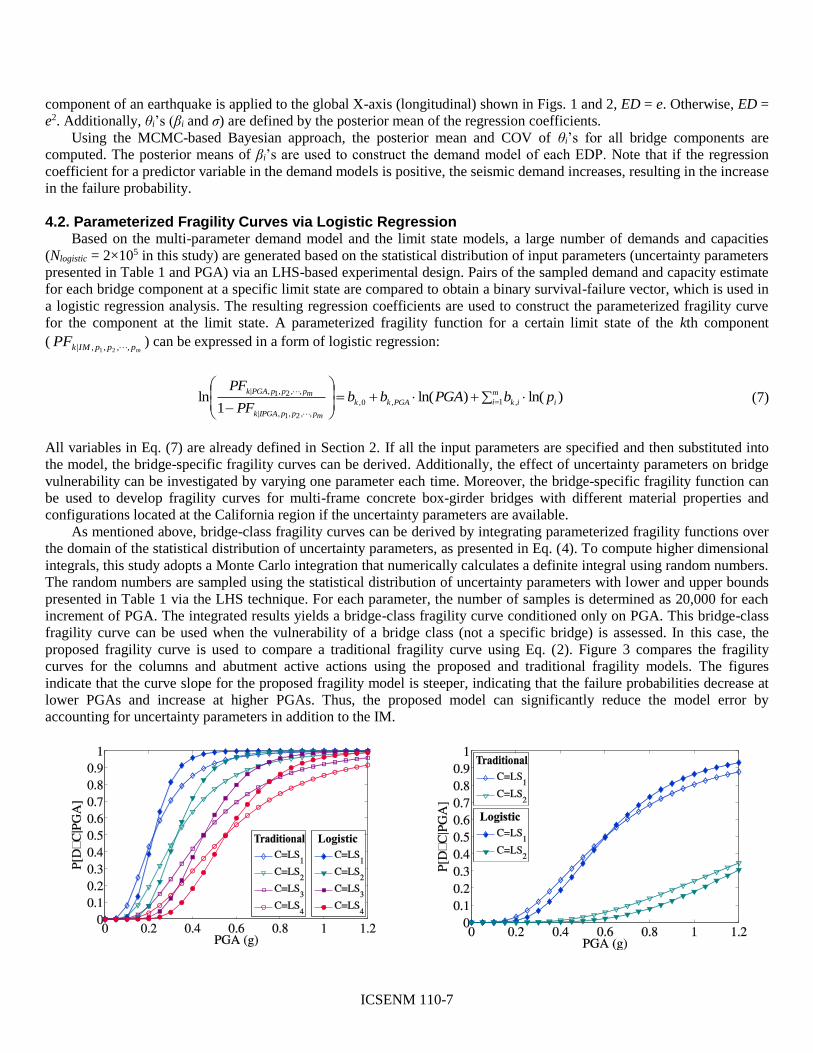
As mentioned above, bridge-class fragility curves can be derived by integrating parameterized fragility functions over

the domain of the statistical distribution of uncertainty parameters, as presented in Eq. (4). To compute higher dimensional

integrals, this study adopts a Monte Carlo integration that numerically calculates a definite integral using random numbers.

The random numbers are sampled using the statistical distribution of uncertainty parameters with lower and upper bounds

presented in Table 1 via the LHS technique. For each parameter, the number of samples is determined as 20,000 for each

increment of PGA. The integrated results yields a bridge-class fragility curve conditioned only on PGA. This bridge-class

fragility curve can be used when the vulnerability of a bridge class (not a specific bridge) is assessed. In this case, the

proposed fragility curve is used to compare a traditional fragility curve using Eq. (2). Figure 3 compares the fragility

curves for the columns and abutment active actions using the proposed and traditional fragility models. The figures

indicate that the curve slope for the proposed fragility model is steeper, indicating that the failure probabilities decrease at

lower PGAs and increase at higher PGAs. Thus, the proposed model can significantly reduce the model error by

accounting for uncertainty parameters in addition to the IM.

ICSENM 110-8

(a) Column (b) Abutment-Active

Fig. 3: Comparison of bridge-class column fragility curves.

5. Conclusion This study proposes a probabilistic framework for facilitating the seismic risk assessment of bridges with the same

bridge class in the transportation network at the specific area. This framework includes the selection of a bridge class,

characterization of bridge attributes such as material and geometric uncertainties, creation of numerical component models,

construction of multi-parameter demand models using a Bayesian parameter estimation method, and development of

bridge-class fragility models using logistic regression. The parameterized fragility models are used (1) to produce bridge-

specific (one-dimensional) fragility curves when the uncertainty parameters are available and (2) to develop bridge-class

(one-dimensional) fragility curves using a Monte Carlo integration. Additionally, the Bayesian approach facilitates

identifying significant uncertainty parameters that affect seismic demands without performing numerous structural

analyses required for design of experiments. Comparison of the proposed and traditional fragility models indicates that the

traditional fragility model overestimates failure probabilities at lower PGAs and underestimates them at higher PGAs. This

proposed framework can be readily implemented into other bridge classes if statistical distributions of uncertainty

parameters based on a bridge inventory analysis are available.

Acknowledgements This research was supported by Basic Research Program in Science and Engineering through the National Research

Foundation of Korea funded by the Ministry of Education (NRF-2016R1D1A1B03933842).

References [1] B. G. Nielson and R. DesRoches, “Seismic fragility methodology for highway bridges using a component level

approach,” Earthquake Eng. Struct. Dyn., vol. 36, pp. 823-839, 2007.

[2] K. N. Ramanathan, J. E. Padgett, and R. DesRoches, “Temporal evolution of seismic fragility curves for concrete

box-girder bridges in California,” Eng. Struct., vol. 97, pp. 29-46, 2015.

[3] J. -S. Jeon, R. DesRoches, T. Kim, and E. Choi, “Geometric parameters affecting seismic fragilities of curved multi-

frame concrete box-girder bridges with integral abutments,” Eng. Struct., vol. 122, pp. 121-143, 2016.

[4] J. Ghosh, J. E. Padgett, and L. Dueñas-Osorio, “Surrogate modeling and failure surface visualization for efficient

seismic vulnerability assessment of highway bridges,” Probabilist. Eng. Mech., vol. 34, pp. 189-199, 2013.

[5] K. Rokneddin, J. Ghosh, L. Dueñas-Osorio, and J. E. Padgett, “Seismic reliability assessment of aging highway

bridge networks with field instrumentation data and correlated failures, II: Application,” Earthquake Spectra, vol.

30, pp. 819-843, 2014.

[6] F. McKenna, “OpenSees: A framework for earthquake engineering simulation,” Comput. Sci. Eng., vol. 13, pp. 58-

66, 2011.

[7] J. -S. Jeon, S. Mangalathu, J. Song, and R. DesRoches, “Parameterized seismic fragility curves for curved multi-

frame concrete bridges using Bayesian parameter estimation,” J. Earthquake Eng., in review, 2016.

[8] Caltrans, Personal communication with the P266, Task 1780 Fragility project panel members including C Roblee, M

Yashinsky, M Mahan, T Shantz, and L Turner, California Department of Transportation. Sacramento, CA, 2015.

[9] O. C. Celik and B. R. Ellingwood, “Seismic fragilities for non-ductile reinforced concrete frames–Role of aleatoric

and epistemic uncertainties,” Struct. Saf., vol. 32, pp. 1-12, 2010.

[10] Caltrans. (2016, October 5). Bridge design practice manual [Online]. Available:

http://www.dot.ca.gov/hq/esc/techpubs/manual/bridgemanuals/bridge-design-practice/bdp.html

[11] Caltrans, Seismic design criteria version 1.7, Office of Structures Design, California Department of Transportation,

Sacramento, CA, 2013.

[12] J. B. Mander, M. J. N. Priestley, and R. Park, “Theoretical stress-strain model for confined concrete,” J. Struct. Eng.,

vol. 114, pp. 1804-1826, 1988.

[13] P. F. Silva, S. Megally, F. Seible, “Seismic performance of sacrificial interior shear keys,” ACI Struct. J., vol. 100,

177-187, 2003.

[14] S. Muthukumar and R. DesRoches, “A Hertz contact model with non-linear damping for pounding simulation,”

Earthquake Eng. Struct. Dyn., vol. 35, pp. 811-828, 2006.

ICSENM 110-9

[15] A. Shamsabadi, P. Khalili-Tehrani, J. P. Stewart, E. Taciroglu, “Validated simulation models for lateral response of

bridge abutments with typical backfills,” J. Bridge Eng., vol. 15, pp. 302-311, 2010.

[16] J. W. Baker, S. K. Shahi, and N. Jayaram, New ground motion selection procedures and selected motions for the

PEER Transportation Research Program, Pacific Earthquake Engineering Research Center, University of

California, Berkeley, CA, PEER Report 2011/03, 2011.